loss minimization control of permanent magnet … thesis in the department of electrical and...
TRANSCRIPT

Loss Minimization Control of Permanent Magnet
Synchronous Machine for Electric Vehicle Applications
KANG CHANG
A Thesis
in
The Department
of
Electrical and Computer Engineering
Presented in Partial Fulfillment of the Requirements
for the Degree of Master in Applied Science
(Electrical & Computer Engineering) at
Concordia University
Montreal, Quebec, Canada
Aug 2013
© Kang Chang, 2013

CONCORDIA UNIVERSITY
SCHOOL OF GRADUATE STUDIES
This is to certify that the thesis prepared
By: Kang Chang
Entitled: “Loss Minimization Control of Permanent Magnet Synchronous Machine
for Electric Vehicle Applications”
and submitted in partial fulfillment of the requirements for the degree of
Master of Applied Science
Complies with the regulations of this University and meets the accepted standards with
respect to originality and quality.
Signed by the final examining committee:
________________________________________________ Chair
Dr. M. Z. Kabir
________________________________________________ Examiner, External
Dr. S. Rakheja (MIE) To the Program
________________________________________________ Examiner
Dr. P. Pillay
________________________________________________ Supervisor
Dr. S. Williamson
Approved by: ___________________________________________
Dr. W. E. Lynch, Chair
Department of Electrical and Computer Engineering
____________20_____ ___________________________________
Dr. C. W. Trueman
Interim Dean, Faculty of Engineering
and Computer Science

III
ABSTRACT
Loss Minimization Control of Permanent Magnet Synchronous Machine
for Electric Vehicle Applications
Kang Chang
With the limits of power source taken into consideration, the efficiency of the
traction drive is of particular importance in the engineering of electric vehicle and plug-in
hybrid electric vehicle (EV/PHEV). Thanks to its high power density, high efficiency and
high torque to weight ratio, Permanent Magnet Synchronous Machine (PMSM)
distinguishes itself from other traction system candidates in the EV/PHEV application
market. This research sets out to explore how the control strategy of PMSM can be
optimized so as to achieve a better efficiency performance of EV/PHEV.
Prior research has put forth Loss Minimization Control Strategy (LMC) and
developed its algorithm by considering a certain operating point. The focus has been
placed on how to approximately solve the optimal current reference from a high order
expression. So far, very limited effort has been made toward a generalized form of LMC
algorithm over the full machine operation region, i.e. constant torque and constant power
region. In this thesis, a generalized relationship between d-q current for the LMC of
PMSM is presented, and maximum torque per ampere (MTPA) and maximum torque per
voltage (MTPV) can be derived as special cases of LMC. The proposed control strategy
shows better response and enhancement of the machine efficiency over full speed range
when compared to conventional control strategies.
In order to develop the control method, the machine operation principle is
discussed first, and the machine model is built for the control purpose. Then based on the

IV
analysis of PMSM operation performance with voltage and current constrains, the
boundary of the machine operating is defined. In the light of literature review, the LMC
is derived from the equivalent model of PMSM by considering the core loss. And the
performance of the LMC is analyzed in detail for both constant torque and constant
power region. In addition, the effects of parameters variation are investigated. Thus the
control strategy is improved by considering full speed range. A Simulink model of
PMSM with core loss taken into consider is developed to test the proposed control
method. The experiment is performed on a lab surface-mounted PMSM. The experiment
results are found to be consistent with simulation results.
V
ACKNOWLEDGEMENTS
I would first express my deepest gratitude to my supervisor, Dr. Sheldon S.
Williamson, for his guidance, patience, trust, and financial support for me to finish this
thesis. Without his firm direction and generous help, I couldn’t have overcome the
obstacles encountered on my way of studying. I am forever indebted to him for giving
me the opportunity to explore this interesting research topic, taking effort to correct my
mistakes, giving me inspiring and constructive advices, and being always available and
responsive to any questions that I have had.
A heartfelt “thank you” also goes to Dr. Pragasen Pillay, who has been a constant
source of knowledge and encouragement throughout my graduate studies. He has instilled
in me a serious attitude towards academic research as well as a will to always pursue the
best along the way in my studies and personal development.
I would also like to express my appreciation to all the friends and colleagues in
the Power Electronics and Energy Research (PEER) group. I must thank Abijit
Choudhury, Lesedi Masisi, Maged Ibrahim, Jemimah C. Akiror, Avrind Rmanan, Manu
Jain and Chirag Desai for their kindness, expertise, and tireless help. These friends will
always remain dear to me.
Last but not the least, I am grateful to my friends Yin, Yue, Lin, Jie and my wife
Jun. Without their love, understanding and support, this work would not have come to
fruition.

VI
TABLE OF CONTENTS
LIST OF FIGURES .......................................................................................................... IX
LIST OF TABLES ........................................................................................................... XII
CHAPTER 1 INTRODUCTION .................................................................................... 1
1.1 PMSM FOR ELECTRIC VEHICLE APPLICATIONS ..................................................... 1
1.2 MOTIVATION AND REVIEW OF TECHNOLOGIES ....................................................... 2
1.3 THESIS OUTLINE ..................................................................................................... 3
CHAPTER 2 FUNDAMENTALS OF PERMANENT MAGNET SYNCHRONOUS
MACHINE 5
2.1 INTRODUCTION ....................................................................................................... 5
2.2 MODELING OF PERMANENT MAGNET SYNCHRONOUS MACHINE ............................ 6
2.2.1 Three phase modeling .............................................................................................................. 7
2.2.2 Reference frame transformation .............................................................................................. 8
2.2.3 Basic mathematic model .......................................................................................................... 9
2.2.4 PMSM Equivalent Electric Circuit ........................................................................................ 12
2.3 ANALYSIS OF PMSM OPERATION ........................................................................ 12
2.3.1 Current and Voltage constrains ............................................................................................ 13
2.3.2 Constant Torque Region ........................................................................................................ 15
2.3.3 Constant Power Region ......................................................................................................... 16
2.3.4 Power-Speed characteristic ................................................................................................... 16
2.4 SUMMARY ............................................................................................................ 18
CHAPTER 3 CONTROL OF PERMANENT MAGNET SYNCHRONOUS
MACHINE 20

VII
3.1 INTRODUCTION ..................................................................................................... 20
3.2 DRIVE SYSTEM OF PMSM .................................................................................... 22
3.3 CONTROL STRATEGIES FOR PMSM ...................................................................... 23
3.3.1 Constant Torque Angle Control ............................................................................................ 24
3.3.2 Unity Power Factor Control (UPF) ...................................................................................... 25
3.3.3 Maximum Torque per Ampere (MTPA) Control .................................................................... 26
3.3.4 Maximum Torque per Voltage (MTPV) Control .................................................................... 28
3.3.5 Flux Weakening Control ........................................................................................................ 30
3.4 SUMMARY ............................................................................................................ 31
CHAPTER 4 LOSS MINIMIZATION CONTROL .................................................... 32
4.1 LITERATURE REVIEW OF LOSS MINIMIZATION CONTROL ..................................... 32
4.2 DEVELOPMENT OF LOSS MINIMIZATION CONTROL ............................................... 35
4.2.1 Losses in PMSM machine ...................................................................................................... 35
4.2.2 Equivalent Circuit Model with Core Losses .......................................................................... 37
4.2.3 Loss Minimization Control .................................................................................................... 39
4.3 PERFORMANCE ANALYSIS OF LMC ...................................................................... 42
4.3.1 Current constraint Operation ................................................................................................ 42
4.3.2 Voltage constraint Operation ................................................................................................ 44
4.3.3 LMC Operation Performance Boundary Regions ................................................................. 45
4.4 GLOBAL SOLUTION FOR EFFICIENCY IMPROVEMENT ............................................ 46
4.4.1 MTPA Derivation .................................................................................................................. 48
4.4.2 MTPV Derivation .................................................................................................................. 48
4.4.3 Global Solution ...................................................................................................................... 49
4.5 LMC STRATEGY OVER ENTIRE SPEED RANGE ...................................................... 50
CHAPTER 5 CONTROL SYSTEM SIMULATION MODEL DEVELOPMENT AND
RESULTS 53
5.1 DEVELOPMENT OF THE SIMULATION MODEL ........................................................ 54
5.1.1 PMSM Model with Core Loss ................................................................................................ 54

VIII
5.1.2 Current Controller Mode....................................................................................................... 55
5.1.3 Speed Controller Model......................................................................................................... 59
5.2 MACHINE MODEL VALIDATION ............................................................................ 61
5.2.1 No-load Test Case Simulation ............................................................................................... 62
5.2.2 Load Disturbance Test Case Simulation ............................................................................... 63
5.2.3 Effect of d-axis Current on Loss Simulation .......................................................................... 64
5.3 LMC SIMULATION ................................................................................................ 66
5.3.1 Steady State Simulation ......................................................................................................... 66
5.3.2 Simulation for Operating Above Base Speed ......................................................................... 68
5.3.3 Transition Simulation ............................................................................................................ 70
5.3.4 Vehicle Drive Cycle Test Case Simulation ............................................................................ 73
5.4 SUMMARY ............................................................................................................ 77
CHAPTER 6 EXPERIMENTAL TESTS AND VERIFICATION .............................. 79
6.1 SIMULATION OF SPM ........................................................................................... 79
6.1.1 No-load Simulation ................................................................................................................ 81
6.1.2 Steady-state Simulation ......................................................................................................... 82
6.1.3 FEA Simulation and Verification........................................................................................... 85
6.2 EXPERIMENTAL TESTING AND VERIFICATION ....................................................... 87
6.2.1 Experimental Test Set-up ....................................................................................................... 88
6.2.2 No-load Test .......................................................................................................................... 89
6.2.3 Steady-state Load Test ........................................................................................................... 90
6.3 DISCUSSION .......................................................................................................... 91
6.3.1 Effect of Core Loss Resistance .............................................................................................. 92
6.3.2 Effect of q-axis Inductance .................................................................................................... 94
6.3.3 Effect of Permanent Magnet Flux .......................................................................................... 97
CHAPTER 7 CONCLUSIONS AND FUTURE WORK ............................................ 98
7.1 CONCLUSIONS ...................................................................................................... 98
7.2 FUTURE WORK ................................................................................................... 100
REFERENCES ............................................................................................................... 101

IX
LIST OF FIGURES
FIGURE 2.1: PERMANENT MAGNET AC MACHINE TOPOLOGIES: (A) SURFACE MOUNTED; (B)
SURFACE INSET; (C) INTERIOR RADIAL; (D) INTERIOR CIRCUMFERENTIAL ..................... 6
FIGURE 2.2: THREE PHASE PMSM AND TWO PHASE PMSM .............................................. 7
FIGURE 2.3. THREE PHASE TO TWO PHASE TRANSFORMATION [10] ..................................... 8
FIGURE 2.4: PMSM EQUIVALENT DQ MODEL CIRCUIT....................................................... 12
FIGURE 2.5. TORQUE-SPEED CHARACTERISTICS ................................................................ 13
FIGURE 2.6. PMSM OPERATION REGION WITH VOLTAGE AND CURRENT CONSTRAINT ...... 15
FIGURE 2.7 POWER-SPEED CHARACTERISTICS OF PMSM: ................................................ 18
FIGURE 3.1. PHASOR DIAGRAM OF THE PMSM ................................................................ 20
FIGURE 3.2 BASIC VECTOR CONTROL BLOCK DIAGRAM .................................................. 22
FIGURE 3.3. CONSTANT TORQUE ANGLE CONTROL PHASOR DIAGRAM ............................... 24
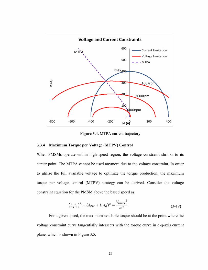
FIGURE 3.4. MTPA CURRENT TRAJECTORY ...................................................................... 28
FIGURE 3.5. MTPV CURRENT TRAJECTORY ...................................................................... 29
FIGURE 3.6: FLUX WEAKENING REGION IN DQ-AXIS CURRENT PLANE ................................ 30
FIGURE 4.1: STEADY-STATE POWER LOSSES IN AN AC MACHINE ...................................... 35
FIGURE 4.2 : EQUIVALENT CIRCUIT OF PMSM INCORPORATING CORE LOSSES .................. 37
FIGURE 4.3 : PLOT OF LOSSES VERSUS D-AXIS CURRENT ................................................... 38
FIGURE 4.4. LMC CURRENT TRAJECTORY FOR VARYING SPEEDS ...................................... 41
FIGURE 4.5: EXAMPLE PLOT OF LMC AND TOTAL LOSSES ................................................ 42
FIGURE 4.6. TORQUE-SPEED CHARACTERISTICS USING LMC UNDER CURRENT CONSTRAINT
.................................................................................................................................... 43
X
FIGURE 4.7: TORQUE-SPEED CHARACTERISTICS USING LMC UNDER VOLTAGE CONSTRAINT
.................................................................................................................................... 45
FIGURE 4.8. LMC OPERATION REGION CONSIDERING BOTH VOLTAGE AND CURRENT
CONSTRAINTS .............................................................................................................. 46
FIGURE 4.9: LMC CURRENT TRAJECTORY AND CONSTANT LOAD ...................................... 50
FIGURE 4.10: FLOW CHART OF EFFICIENCY ENHANCEMENT CONTROL STRATEGY ............. 51
FIGURE 5.1: BLOCK DIAGRAM OF A BASIC DRIVE SYSTEM ................................................. 53
FIGURE 5.2. PMSM SIMULINK MODEL ............................................................................ 55
FIGURE 5.3 : CURRENT CONTROLLER ................................................................................ 56
FIGURE 5.4: D-AXIS CURRENT LOOP FOR PI TUNING .......................................................... 56
FIGURE 5.5: UNITY FEEDBACK CURRENT LOOP ................................................................. 57
FIGURE 5.6: BODE PLOT AND STEP RESPONSE OF CURRENT LOOP ...................................... 58
FIGURE 5.7: SPEED LOOP WITH UNITY FEEDBACK .............................................................. 59
FIGURE 5.8: BODE PLOT AND STEP RESPONSE OF CURRENT LOOP ...................................... 61
FIGURE 5.9: PMSM DRIVE SYSTEM IN SIMULINK ............................................................. 61
FIGURE 5.10: NO-LOAD SPEED RESPONSE SIMULATION RESULTS ...................................... 63
FIGURE 5.11: LOAD DISTURBANCE RESPONSE SIMULATION RESULTS ................................ 64
FIGURE 5.12. EFFECT OF THE D-AXIS CURRENT ON LOSS SIMULATION ............................... 65
FIGURE 5.13: STEADY STATE SIMULATION FOR LMC ....................................................... 67
FIGURE 5.14: OPERATING POINT OF FWC, LMC, AND MTPV .......................................... 68
FIGURE 5.15: SIMULATION COMPARISON OF MTPV, FWC, AND LMC ............................. 70
FIGURE 5.16: TRANSITION SIMULATION RESULTS ............................................................. 72
FIGURE 5.17: TRANSITION SIMULATION CURRENT TRAJECTORY ....................................... 73

XI
FIGURE 5.18: SPEED AND TORQUE PROFILE OF DRIVE CYCLE ............................................ 74
FIGURE 5.19: DRIVE CYCLE SIMULATION RESULTS............................................................ 75
FIGURE 5.20: DRIVE CYCLE SIMULATION CURRENT TRAJECTORY ..................................... 76
FIGURE 6.1: CORE LOSSES RESISTANCE ............................................................................. 80
FIGURE 6.2: NO-LOAD SIMULATION OF LAB SPM ............................................................. 81
FIGURE 6.3: 1000RPM WITH FULL LOAD SIMULATION OF LAB SPM ................................. 83
FIGURE 6.4: 1600RPM AND 2000RPM WITH FULL LOAD SIMULATION RESULTS .............. 85
FIGURE 6.5: FEA TOTAL LOSS PLOT FOR 1000RPM, 1600RPM, AND 2000RPM ................... 87
FIGURE 6.8: EXPERIMENT SETUP BLOCK DIAGRAM ........................................................... 88
FIGURE 6.9: INPUT POWER RESULT FOR VARIED ID ............................................................. 89
FIGURE 6.10: INPUT POWER WAVEFORM FOR ID = -0.2A, -0.4A AND -0.6A ....................... 90
FIGURE 6.11: STEADY-STATE LOAD TEST RESULTS ........................................................... 91
FIGURE 6.12. EFFECT OF CORE LOSS RESISTANCE ON THE TOTAL LOSS .............................. 92
FIGURE 6.13: LMC WITH VARIATION OF RC ...................................................................... 93
FIGURE 6.14: LMC WITH VARIATION OF RS ....................................................................... 94
FIGURE 6.15. EFFECT OF Q-AXIS INDUCTANCE ON THE TOTAL LOSS .................................. 95
FIGURE 6.16: LMC WITH VARIATION OF LQ...................................................................... 96
FIGURE 6.17: LMC WITH VARIATION OF LD ...................................................................... 96
FIGURE 6.18: LMC WITH VARIATION OF PM FLUX ........................................................... 97

XII
LIST OF TABLES
TABLE 1-1: ADVANTAGE (GREEN) AND DISADVANTAGE (RED) OF THE MAJOR MOTOR TYPES
[3] ................................................................................................................................. 2
TABLE 5-1: PARAMETERS OF MODELED MACHINES .......................................................... 53
TABLE 6-1: PROTOTYPE SPM PARAMETERS ..................................................................... 79
TABLE 6-2: FEA RESULTS AND CORE LOSSES RESULTS ..................................................... 80
TABLE 6-3: FEA SIMULATION RESULTS ............................................................................ 86
TABLE 6-4: EXPERIMENT PARAMETERS ............................................................................. 88

1
CHAPTER 1 INTRODUCTION
1.1 PMSM for Electric Vehicle Applications
Recent years have seen growing awareness of the risks associated with global warming,
environmental pollution and nature resource crisis of the Earth. Being a major consumer
of petroleum and a key contributor to carbon dioxide emissions, the transportation plays
an important role in addressing those environment-related and energy-related issues.
Electric vehicle (EV) and plug-in hybrid electric vehicles (PHEV) have been proposed to
replace conventional fossil-fuel combustion vehicles, and progress is under way. Up to
today, there have already been many commercial EV/PHEVs on the road. Among the
most successful examples there are Toyota prius, Chevlet volts, and Nissan Leaf.
Speaking of electric vehicle application, the standards of choosing an appropriate
traction motor for the EV/PHEV propulsion are often focused on the characteristics such
as torque density, extended speed range, energy efficiency, safety and reliability, thermal
cooling, and cost. As determined by vehicle dynamics and system architecture, the
extended speed range ability and energy efficiency are two particularly important factors
in selecting the propulsion motor [1]. In addition, the power source in EV/PHEV is the
battery, whose performance is claimed by many as “Achilles Heel” of any EV/PHEV
application. The traction drive system consumes the largest share of the power source,
and its efficiency thus becomes vital for EV/PHEV application. Generally, the drive
system includes power inverter and traction motor. In order for the whole system to
achieve high efficiency, it is essential that both the power inverter and the traction motor

2
operate with their optimal efficiency throughout the driving schedule [2]. This thesis
work will emphasize on the traction motor part.
There are many types of machine that are considered as candidates for electric
vehicle traction system, which mainly include induction motor (IM), permanent magnet
synchronous machine (PMSM), and switch reluctance machine (SRM). It is noteworthy
that due to its high efficiency, power density and torque-inertia ratio, PMSM has now
become the most common choice in the EV/PHEV. Table 1.1 shows the most important
features of the principal motor types that are being considered for EV/PHEV application.
Motor Design Induction
(natural
field
weakening)
PM SR
SPM motor
(BLDC)
SPM motor with
concentrated
windings
IPM motor Non-linear
solenoid type
force
CPSR 4 11 Theotetically,
infinity, but
allow for
rotational losses
Theotretically,
infinity, but
allow for
rotational losses
Discontinuous
control
Cost $ $$ $$ $$$ $
Peak Power to
Weight Ratio
Low High High Highest Low
Peak Power to
Volume Ratio
Low High High Highest Low
Lifetime Higher High High High Higher
Table 1-1: Advantage (green) and disadvantage (red) of the major motor types [3]
1.2 Motivation and Review of Technologies
In order to improve the efficiency of the machine, emphasis is often placed on the
machine design. With proper topology of the machine and improvement of the material,
the total efficiency can be optimized. It can also be enhanced by way of employing
automatic control strategy. There has been a lot of research focused on the automatic
control method, which mainly include maximum torque per ampere control (MTPA) that
is meant to minimize the copper loss [4], maximum torque per voltage control (MTPV)
3
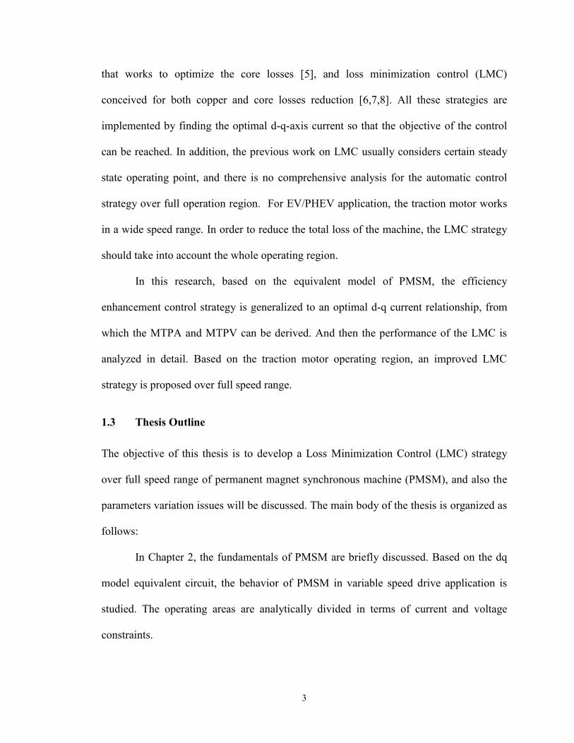
that works to optimize the core losses [5], and loss minimization control (LMC)
conceived for both copper and core losses reduction [6,7,8]. All these strategies are
implemented by finding the optimal d-q-axis current so that the objective of the control
can be reached. In addition, the previous work on LMC usually considers certain steady
state operating point, and there is no comprehensive analysis for the automatic control
strategy over full operation region. For EV/PHEV application, the traction motor works
in a wide speed range. In order to reduce the total loss of the machine, the LMC strategy
should take into account the whole operating region.
In this research, based on the equivalent model of PMSM, the efficiency
enhancement control strategy is generalized to an optimal d-q current relationship, from
which the MTPA and MTPV can be derived. And then the performance of the LMC is
analyzed in detail. Based on the traction motor operating region, an improved LMC
strategy is proposed over full speed range.
1.3 Thesis Outline
The objective of this thesis is to develop a Loss Minimization Control (LMC) strategy
over full speed range of permanent magnet synchronous machine (PMSM), and also the
parameters variation issues will be discussed. The main body of the thesis is organized as
follows:
In Chapter 2, the fundamentals of PMSM are briefly discussed. Based on the dq
model equivalent circuit, the behavior of PMSM in variable speed drive application is
studied. The operating areas are analytically divided in terms of current and voltage
constraints.

4
In Chapter 3, various control strategies are discussed. The maximum torque per
ampere (MTPA), maximum torque per voltage (MTPV) and flux-weakening method are
derived based on the dq equivalent model. Also, their performances are analyzed from
efficiency enhancement point of view.
In Chapter 4, the loss minimization control (LMC) strategies of PMSM are
reviewed. With the core loss taken into consideration, the dq model with core loss
resistance is used to derive the LMC. A generalized optimal current relationship is
presented. And then by taking into account both constant torque and constant power
region, the performance of LMC is analyzed in detail. Also, the effects of the machine
parameters are examined. At the end, an improved control strategy is proposed over full
speed range based on the performance of the LMC.
In Chapter 5, the simulation model is developed by using Matlab. The
performance and results of the simulation are analyzed.
In Chapter 6, a lab design surface-mounted PMSM is used to test the proposed
algorithm. The experimental results are compared with the simulation results and
discussed in detail. In particular, the parameter variation issue is addressed in the
discussion.
Chapter 7 concludes the thesis and proposes future research work.

5
CHAPTER 2 FUNDAMENTALS OF PERMANENT MAGNET
SYNCHRONOUS MACHINE
2.1 Introduction
The permanent magnet (PM) materials with considerable energy density were firstly
introduced into the designing of electrical machine during 1950s. They have experienced
rapid growth and continuous improvement, especially during the past few years. Instead
of field windings, the PM poles in rotor provide electromagnetic field and thus eliminate
slip rings and brush assembly. Equally mentionable is that electronic commentators
replace traditional mechanical ones in modern power electronics. These two factors have
jointly propelled the development and growth of PM AC machine in the last two decades.
It has now become possible to build high performance drive systems in a wide range of
application fields including but not limited to electric vehicles.
Generally, the PM AC machine can be classified by the direction of the flux
density distribution. Its two main categories are radial field PM machines and axial field
ones [9]. Also, depending on their induced back-EMF shape, the radial fields PM
machines are classified into PMSM with sinusoidal back-EMF and BLDC with
trapezoidal back-EMF. The discussion in this research is based on the PMSM only.
According to the location of the permanent magnet in the rotor, there are four topologies
as shown in Figure 1.

6
Figure 2.1: Permanent Magnet AC machine topologies: (a) Surface mounted; (b) Surface
inset; (c) Interior radial; (d) Interior circumferential
In today’s EV/PHEV application market and related research, the interior radial
PM machine (IPM) gets increasing attention. Compared with other topologies, this kind
of PMSM has less torque ripple and higher reliability because of its buried magnets.
Also, the buried magnet is better protected from demagnetizing due to the armature
reactance. Moreover, the IPM features a special configuration in rotor. It results in a very
strong saliency, which contributes to the total load demand by additional reluctance
torque. Furthermore, the strong saliency feature provides an excellent flux weakening
capability, and thus enables a wide range of high speed operation suitable for EV
application. As the counterpart, the surface mounted topology PMSM (SPM) can be seen
as a special case of IPM. This chapter will derive the model of PMSM based on IPM.
2.2 Modeling of Permanent Magnet Synchronous Machine

7
In order to develop the desired algorithm, the behavior of the PMSM should be explored
based on the dynamic model of the machine. In this section, the modeling of PMSM is
derived from the transformation theory. And the d-q rotor reference frame model will be
used for the analysis of PMSM.
2.2.1 Three phase modeling
The PMSM can be modeled in three phase stator coordinates with winding as shown in
Figure 2. The two phase coordinates is also shown in Figure 2.
Figure 2.2: Three Phase PMSM and Two Phase PMSM
The voltage equations are
(2-1)

8
where are stator phase voltages, are stator phase currents, and
are the phase flux linkages. The input power for this model is
(2-2)
Since the variables in this model are all sinusoidal or rotor position dependent, the
solution of these equations will be computational complex.
2.2.2 Reference frame transformation
As one kind of observer platforms, the reference frame offers a unique view of the
system. A simplified model with constant variables is desirable for the purpose of
control. In PMSM, rotor frame revolves at the synchronous speed with stator sinusoidal
supply frequency. As a result, sinusoidal variable can be perceived as dc signal from the
rotor frame. Based on this rotor reference frame, a two-phase motor can be derived from
the three-phase model in direct and quadrature axes, which is generally referred to as d-q
axes model. Figure 3 shows the stator abc phase and the rotating dq phase winding.
Figure 2.3. Three phase to two phase transformation [10]

9
By applying Park’s transformation, the voltage equation in three-phase model can
be transferred to the dq rotating frame as following:
[
]
[
]
[
]
(2-2)
where is the rotor angle.
The Park’s transformation is represented as:
[ ]
[
]
(2-3)
and its inverse form is
[ ]
[
]
(2-4)
This transformation is also applicable to the current and flux linkage.
2.2.3 Basic mathematic model
After applying Park’s transformation, the synchronous machine variables in the abc phase
equation are transferred to the dq-variable in the rotor reference frame. Since the
reference frames are moving at an angular speed equal to the angular frequency of the
sinusoidal supply, all sinusoidally varying inductances in the abc frame become constant
in the dq frame.

10
With the assumption of saturation being neglected and the sinusoidal back emf,
the dq equation in the rotor reference frame of the PMSM are derived as
(2-5)
The electromagnetic torque is expressed as
[ ]
(2-6)
It can be seen that the developed electromagnetic torque includes two components. The
first term corresponds to the magnet exciting torque, which is the reaction between q-axis
current and the permanent magnet on rotor. The second term is the feature of IPM, which
is the reluctance torque due to the difference in the d-q-axis inductance.
In terms of mechanical load, the torque is
(2-7)
In the state space form, the PMSM model can be expressed as:
(2-8)
where
: q-axis and d-axis voltage
: q-axis and d-axis current
: stator phase resistance
: q-axis and d-axis inductance
: derivative operator

11
: permanent magnet flux
: electromagnetic torque and load torque
: number of poles
: the moment of inertia of the load and machine combined
: the friction coefficient of the load and machine
: the mechanical and electrical rotor speed,
Alternatively, the dynamic equations of the PMSM in rotor reference frame can
be represented by using flux linkages as variables. The flux linkages are continuous no
matter voltage and current are continuous or not. In so doing, it is possible to differentiate
the variables with numerical stability. This alternative way of representing the PMSM
dynamic equations also places emphasis on how the flux and torque channels are dis-
coupled.
The model in flux linkage is defined as
(2-9)
where
(2-10)
and the electromagnetic torque is
[ ]
(2-11)
From the power equivalence condition, the input power in terms of d-q variable, it is
(2-12)

12
2.2.4 PMSM Equivalent Electric Circuit
From the dynamic equation, the equivalent circuit of PMSM can be drawn as shown in
Figure 4. There are two ciruits representing dynamic q-axis circuit and d-axis equivalent
circuit.
Rs Ld
ωLqiqVd
id
Rs Lq
ω(Ldid+λPM )Vq
iq
Figure 2.4: PMSM equivalent dq model circuit
The models can be used to examine both the transient and steady state behaviors
of PM machine drive system.
2.3 Analysis of PMSM Operation
For EV/PHEV application, the traction motor drives are generally designed to provide a
constant torque up to base speed and constant power for extended speed up to a
maximum speed. The torque speed characteristic is plotted as Figure 2.5:

13
Figure 2.5. Torque-Speed characteristics
For the purpose of developing the control strategy of PMSM, the performance of
PMSM is analyzed based on the d-q-axis model with the assumption ignoring the voltage
drop on phase resistance and core loss. The control strategies and performance features in
different regions will be discussed in detail.
2.3.1 Current and Voltage constrains
According to the equivalent circuit mentioned in section 2.2.4, the two-phase mathematic
model in steady state is written as:
[
] [
] [
] [
]
(2-13)
And the torque produced by the machine is:
[ ]
(2-14)
Speed
Constant
Torque Region
Constant
Power Region
Torque

14
For the inverter-fed drive system with DC battery source, there are voltage and current
constraints due to the power rating of the inverter, machine and power source. The
current constraint is identified as:
(2-15)
where Is,max is the maximum phase current of the machine. It is a circle in the dq current
plane.The voltage constraint is:
(2-16)
By ignoring the voltage drop on the phase resistance, in terms of dq current, it is:
( )
(2-17)
where Vs,max is the maximum available voltage provided by the inverter. Generally,
√
(2-18)
where Vdc is the dc power source voltage. For given speed, the voltage constraint is an
ellipse with center (
, 0) in the dq current plane. With the speed increasing, the
ellipse shrinks to the center. As shown in Figure 2.6, the above constraints are plotted in
id-iq plane by using one example IPM.

15
Figure 2.6. PMSM operation region with voltage and current constraint
Due to the current and voltage constraints, the operation region of the machine
has to be within the overlapped area of the current and voltage constraints.
2.3.2 Constant Torque Region
In constant torque region, since the speed is lower than the base speed, the voltage
constraint will not be exceeded in most cases. More concern will be placed on the
current constraint. In order to fully utilize the current, maximum torque per current
control strategy is widely employed, which assures the minimization of the copper loss.
Under this control strategy, the highest available speed is given by
√( )
(2-19)
where Id, Iq are the MTPA optimal current for the peak torque, and
(2-20)
-600
-400
-200
0
200
400
600
-1000 -800 -600 -400 -200 0 200 400 600Iq (
A)
Id (A)
Voltage and Current Constraints
Current Limitation
Voltage Limitation
Imax w1
w2
w3
w1<w2<w3
(-
,0)

16
Below the speed , the motor can be accelerated by this peak torque.
2.3.3 Constant Power Region
When the speed exceeds the rated speed, the voltage constraint will be reached, and the
operation of machine enters into the constant power region. With appropriate stator
current distribution, the stator flux linkage gets reduced, and high speed operation can be
performed up to extended speed range. In this region, flux weakening control strategy
such as maximum output power, MTPV or LMC is applied for the purpose of the control.
2.3.4 Power-Speed characteristic
Considering the power capacity versus speed of the PMSM, there are three cases be
summarized from [11, 12]. It can be seen that from the voltage constraint equation, the
eclipse center is on (
, 0). With different design flux linkage of the permanent
magnet, d-axis inductance and the available maximum phase current, the power speed
characteristic will be varied.
Case 1:
, which means that the permanent magnet flux is greater than
the maximum d-axis flux field as caused by maximum phase current in stator. Under this
circumstance, the voltage eclipse center is located outside the current constraint circle.
There is a maximum available speed occurring where the two curves tangentially
intersect at point ( , 0). This maximum available speed is called by many as critical
speed, which is expressed as:
(2-20)

17
After that speed, there are no overlapped region between voltage and current constraint.
The power in this case drops fast to zero when the rated speed is exceeded.
Case 2:
, which means that the voltage eclipse center lies on the
current constraint circle. In this case, there is always an overlapped region between them
at any high speed. The constant power region will be theoretical infinite.
Case 3:
, which means that the stator field can cancel the rotor
permanent magnet field in certain phase current that is lower than the maximum phase
current. In this case, the voltage constraint eclipse center goes into the current constraint
circle. It can have infinite constant power region but lower output power compared with
Case 2. The power versus speed characteristics are as shown in Figure 2.7:
iq
id
I-limitV-limit
- 𝑀
wc
Power
Speed
(a)

18
iq
id
I-limitV-limit
- 𝑀
Power
Speed
(b)
iq
id
I-limitV-limit
- 𝑀
Power
Speed
(c)
Figure 2.7 Power-speed characteristics of PMSM:
(a) Case 1, (b) Case 2, (c) Case 3
For EV/PHEV applications, Case 2 and Case 3 are the preferred designs of
PMSM, due to extended constant power region. In this thesis, the LMC control strategy is
developed based on this preferred design of PMSM.
2.4 Summary
In this chapter, the fundamentals of PMSM are presented. The modeling in two axes
coordinate shows a convenient way to understand the behavior of PMSM. And from the

19
control point of view, the variable in dq-axis coordinate becomes dc value, and it is
possible to make the control of PM AC machine as that of DC machine. Based on the two
axes model, the dynamic mathematic equations for PMSM are derived. The equivalent
electrical circuit is also presented in this chapter. Considering the operating region of
PMSM, an analysis is performed at the end of this chapter. Due to voltage and current
constraints, the control of inverter fed PMSM drive should be properly developed to meet
with the objective within the constrained region.

20
CHAPTER 3 CONTROL OF PERMANENT MAGNET
SYNCHRONOUS MACHINE
3.1 Introduction
With optimized design of PMSM, an appropriate control strategy will help extract full
performance capability from the machine. Vector control, also known as field oriented
control or decoupling control, was first proposed by Blaaske [13] and has been widely
applied to the induction motor (IM). It has enabled the controlling of an AC machine like
a separately excited DC machine by the orientation of the stator mmf or current vector in
relation to the rotor flux to obtain the independent control of flux and torque. For
PMSMs, the vector control can also be applied, and it is easier to implement thanks to the
absence of slip frequency current [14]. In this chapter, the vector control for PMSM will
be presented, and different control strategies will be discussed.
From the dq-axes model of PMSM, the phasor diagram of the PMSM is shown as
Figure 3.1.
Figure 3.1. Phasor Diagram of the PMSM

21
Considering the current as input, the three phase currents are:
(
)
(
)
(3-1)
where is the electrical rotor speed, and is the angle between the rotor filed and stator
current pharos and is known as the torque angle.
In the rotor reference frame, the dq-axes stator currents are obtained by applying
Park’s transformation as:
[
]
[
] [
]
(3-2)
Then the dq-axes currents in rotor and stator reference frame are obtained as:
[ ] [
] [ ]
[
] [
]
(3-2)
where are the torque producing current and the flux producing current
respectively. It should be noted that the dq-axes currents are constants in rotor reference
frames, and the torque angle is a constant for a given load torque. Substitute the above
dq-axes stator current in rotor reference frame into torque expression, the torque is
expressed in terms of the stator current magnitude and torque angles as:
[
]
(3-3)

22
Obviously, the control variables stator current magnitude and the torque angle determine
the electromagnet torque with the machine parameters being assumed as constant. In
addition, the mutual flux linkages in the air gap are the result of the rotor flux linkages
and the stator flux linkages. It is given as:
√ ( )
(3-4)
So from the perspective of control, by way of controlling the phase angle and
magnitude of the current phasor from the inverter, which means the dq-axis current in
two phase model on rotor reference frame, the torque can be determined and its control is
achieved accordingly. The PMSM drive is shown to be analogous to the separately
excited dc motor drive. It is achieved by finding the flux and torque producing
components of stator current. And the independent control of electromagnetic torque and
mutual flux is exercised via the flux and torque producing component current.
3.2 Drive System of PMSM
The general block diagram of vector control drive system is shown as in Figure 3.2.
Speed
Controller
iq current
Controller
id current
Controller
d-q current
reference
calculation
Decoupling and
dq to abc
transformation
SVPWM
InverterPMSM
abc to dq
transformation
w
Te*
iq*
id*
iq
id
iabcid,iq
Vq*
Vd*
w
Vabcw*
Figure 3.2 Basic Vector Control Block Diagram

23
There exist two control loops in the drive system. The inner loop is torque loop,
and the outer loop is speed loop. Depending on how the torque is controlled, the inner
loop can be implemented by indirect torque control mode or direct torque control mode.
Indirect torque control is also called stator current vector control or field oriented
current control (FOC) in some literature. The torque equation (3-3) explains the
relationship between the stator phase current and the instantaneous torque. Then the
torque can be controlled by phase current and torque angle, in other words, the dq-axes
current in two phase axes coordinate. For this control mode, the rotor position is needed
except the current sensor. The process of deriving the torque component current and flux
component current references plays a key role in this control. For the control purpose,
different strategies to derive the dq current reference can be applied, for examples,
MTPA, MTPV, and LMC.
Direct torque control was first introduced for the induction motor by [15]. It is of
great interest to EV/PHEV application, especially for dual motor propulsion system,
where the fast torque response is desirable [16]. For PMSMs, direct torque control is also
useful. Based on the torque and flux linkage error between the command and estimations,
the controller outputs proper voltage vectors command to inverters. This control mode
eliminates the current loop and directly controls the torque and flux independently. The
torque and flux ripple are the major problems of this control mode. In some research
work, these problems are tackled with introducing additional PI-controller, which makes
the direct torque control have the same system complexity and the same cost as the
indirect torque control.
3.3 Control Strategies for PMSM

24
Vector control provides the decoupling between torque and flux channel in the PMSM.
The control variables include current, voltage, flux, and torque angle. As the application
requirements vary, there are different control strategies accordingly.
3.3.1 Constant Torque Angle Control
Constant torque angle control, also called zero d-axis current control, is widely used
across the industry. As the phasor diagram in Figure3.3 shows, when torque angle is
maintained at , the direct field component of stator current is brought to zero, and all
the stator current is used to produce torque.
Figure 3.3. Constant torque angle control phasor diagram
The torque control is then the simplified result in the linear relationship between
torque and current as
(3-5)
where is the magnitude of the stator current phasor.
Under this mode, the steady state voltage equations in rotor reference frame as
=90

25
(3-6)
This provides a simple linear torque control, and it is similar to the DC motor control.
The flux linkage under this control is
√ ( )
(3-7)
It reveals that a weakening of mutual flux linkages is out of the question. Thus it only
works for the speed lower than base speed operating range. Also for IPMSM, the
reluctance torque is not utilized.
3.3.2 Unity Power Factor Control (UPF)
UPF control refers to the optimization of the VA rating of the inverter by way of keeping
the power factor at UNITY (1.0). This type of control implies the utmost use of the real
power input to the PMSM. It is enforced by controlling the torque angle as a function of
the motor variables. As shown in Figure 3.1, the angle between the d-axis voltage and q-
axis voltage is
(3-8)
In UPF, the power factor angle has to be zero ( ), which means that the voltage
angle equals to the current angle.
Substitute the voltage in terms of current into equation (3-8)
(3-9)
From the above equation, the torque angle is solved as
(
√
)
(3-10)

26
It should be noted that the torque angle needs to exceed 90°. Otherwise, the
mutual flux linkages might be enhanced and saturation might be observed in the machine,
which is undesirable from the perspective of loss control. In addition, the UPF control
strategy has a very low torque per unit current ratio, and its efficiency will be inferior to
that of other control strategies due to the increasing copper loss for producing the given
torque.
3.3.3 Maximum Torque per Ampere (MTPA) Control
For the IPMSM, the electromagnetic torque is represented as:
[ ]
(3-11)
It is composed of two terms. The former corresponds to the excitation torque by rotor
permanent magnet, which is also called synchronous torque. The second term
corresponds to the reluctance torque, which is the result of the difference in d-q-axis
reluctance. Based on this equation, a strategy enabling the full utilization of the torque
capacity can be derived, which is called maximum torque per ampere control (MTPA). It
provides a maximum electromagnetic torque for a unit stator current via torque angle
control and therefore minimizes copper loss for a given torque. By manipulating the
torque equation (3-11) with the relationship between d-q-axis current and stator current:
(3-12)
Rewrite the equation (3-12) as:
[
]
(3-13)
27
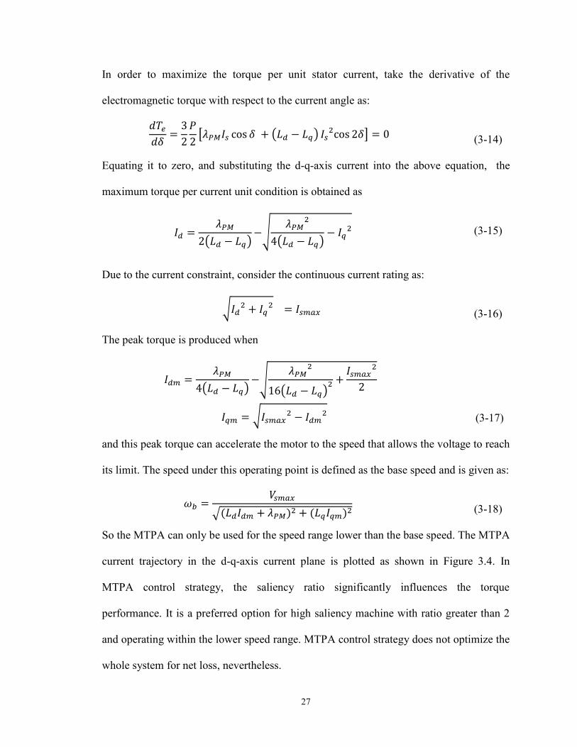
In order to maximize the torque per unit stator current, take the derivative of the
electromagnetic torque with respect to the current angle as:
[ ( )
]
(3-14)
Equating it to zero, and substituting the d-q-axis current into the above equation, the
maximum torque per current unit condition is obtained as
( ) √
( )
(3-15)
Due to the current constraint, consider the continuous current rating as:
√
(3-16)
The peak torque is produced when
( ) √
( )
√
(3-17)
and this peak torque can accelerate the motor to the speed that allows the voltage to reach
its limit. The speed under this operating point is defined as the base speed and is given as:
√
(3-18)
So the MTPA can only be used for the speed range lower than the base speed. The MTPA
current trajectory in the d-q-axis current plane is plotted as shown in Figure 3.4. In
MTPA control strategy, the saliency ratio significantly influences the torque
performance. It is a preferred option for high saliency machine with ratio greater than 2
and operating within the lower speed range. MTPA control strategy does not optimize the
whole system for net loss, nevertheless.
28
Figure 3.4. MTPA current trajectory
3.3.4 Maximum Torque per Voltage (MTPV) Control
When PMSMs operate within high speed region, the voltage constraint shrinks to its
center point. The MTPA cannot be used anymore due to the voltage constraint. In order
to utilize the full available voltage to optimize the torque production, the maximum
torque per voltage control (MTPV) strategy can be derived. Consider the voltage
constraint equation for the PMSM above the based speed as:
( )
(3-19)
For a given speed, the maximum available torque should be at the point where the
voltage constraint curve tangentially intersects with the torque curve in d-q-axis current
plane, which is shown in Figure 3.5.
0
100
200
300
400
500
600
-800 -600 -400 -200 0 200 400
Iq (
A)
Id (A)
Voltage and Current Constraints
Current Limitation
Voltage Limitation
MTPA
Imax
1667rpm
2600rpm
6000rpm
MTPA

29
Figure 3.5. MTPV current trajectory
The voltage constraint equation can also be rewritten in terms of d-q flux linkage:
(3-20)
where
(3-21)
Then rewrite the torque equation with voltage constraint as
[
]
(3-22)
Taking the differentiation with respect to the angle and equating it to zero, the MTPV
optimal current trajectory satisfies the relationship as
( ) [ (
)
] (
)
(3-23)
0
100
200
300
400
500
600
-800 -600 -400 -200 0 200 400
Iq (
A)
Id (A)
Voltage and Current Constraints
Current Limitation
Voltage Limitation
MTPV
1667rpm
2600rpm
6000rpm
MTPV

30
It is plotted in the dq current plane as shown in Figure 3.5. From the observation, it can
be noted that the MTPV curve is independent of a specific speed, and then there is only
one MTPV curve depending on machine parameters. The minimum speed for MTPV
control strategy is determined by the intersect point between the MTPV curve and the
current constraint circle. Below that speed, the intersect point will be outside the current
constraint circle. MTPV control strategy makes full utilization of voltage, which means
minimizing the core losses of the machine.
3.3.5 Flux Weakening Control
When operating above base speed, the backEMF of PMSMs can be exceeding the
available maximum voltage fed by the inverter. In order to enable the speed to exceed the
base speed, a negative d-axis current can be applied to reduce the stator flux linkage and
then decrease the back EMF. It is generally called flux weakening control. This control
strategy allows the machine to work at a speed up to maximum speed, but with a
decreasing maximum available torque.
Figure 3.6: Flux weakening region in dq-axis current plane
0
100
200
300
400
500
600
-500 -400 -300 -200 -100 0
Iq (
A)
Id (A)
Voltage and Current Constraints
Current LimitationVoltage LimitationMTPAMTPVFWC Imax
1667rpm
2600rpm
6000rpm
MTPA
MTPV FWC

31
The flux weakening region is plotted in Figure 3.6, and it is located between the MTPA
and MTPV curves. Different flux weakening control strategies are proposed to meet with
different objectives of the control. Two examples in this regard are efficiency
enhancement flux weakening control [17] and current-voltage constraint maximum
power flux weakening control [18].
3.4 Summary
In this chapter, the vector control of PMSMs is described, and different control strategies
are discussed. As determined by the constraints of voltage and current, the operation of
PMSMs can be divided into three regions with corresponding control strategies. When
the machine runs below the base speed, the MTPA can be applied to obtain maximum
constant torque, and the copper loss can be minimized. After the speed goes above base
speed, the machine enters the flux weakening region. With properly flux weakening
control strategy, the speed can be extended to high speed range with constant output
power. Once the speed reaches some high value, the MTPV control strategy is used to
fully utilize the voltage fed by the inverter, and the core losses will be minimized.

32
CHAPTER 4 LOSS MINIMIZATION CONTROL
For EV application, the efficiency of the whole drive system is the most concerned issue,
especially because of the limited power supply by the battery. In this chapter, the loss
minimization control (LMC) will be discussed, and the pertinent control design will be
investigated in detail.
4.1 Literature Review of Loss Minimization Control
In the PMSM operation, there are numerous combinations of motor variables such as
voltage and current at a given operating point. These combinations result in different total
loss, and the one causing minimum loss is chosen. The loss minimization control (LMC)
has so far received a lot of attention from research on DC machine, induction machine,
and PMSM machine.
Roy S. Colby et al. [19] presented a testing efficiency optimizing controller for
non-salient, scalar controller PMSM. In this approach, the output voltage of the inverter
was adjusted to minimize the DC link current with the motor speed being maintained
constant by independent open loop control of the inverter frequency. The DC link current
rather than the input power to the motor drive was reduced. Due to the nature of the open
loop, the dynamic performance of this approach was not satisfactory for high
performance application.
S. Morimoto et al. [20] established a loss minimization control based on the
equivalent circuit including an iron loss model and a copper loss one. By way of taking
differentiation of the loss function with respect to d-axis current, the optimal d-axis
current was obtained. However, the expression after differentiation is a fourth order

33
equation, which only can be solved analytically for non-saliency. For rotor saliency, it
has to use numerical solution to find optimal value. The machine parameter variation was
not taken into account in this research.
C. C. Chan, K. T. Chau et al. [21] proposed a PMSM machine for mini-EV and
developed a new PWM algorithm, namely equal-area pulse-width modulation
(EAPWM), for the purpose of control. The PWM algorithm can be automatically
adjusted for a varying DC link voltage. It has low harmonic content, and allows a real-
time calculation of the PWM pattern. By employing the new PWM algorithm, the
researchers developed a search algorithm to increase the efficiency of the PMSM. Since
the search algorithm was not dependent on the loss model of the machine, it was not
sensitive to variations in the motor parameters.
Sadegh Vaez, V. I. John, M. A. Rahman et al. [22] proposed an online adaptive
loss minimization controller (ALMC) for interior permanent magnet motor drive. This
control minimizes the total input power to the drive system through continuing
adjustment of d-axis current until the optimal point was found. Compared to the
conventional stepwise change, the ALMC offers advantages such as very smooth
performance and fast searching time.
C. Cavallaro et al. [23] developed an online loss minimization algorithm based on
the model proposed by S. Morimoto et al. [20]. With the use of a substantial binary
search algorithm, the d-axis current was adjusted until the total loss was minimized for a
given operating point.
Juggi Lee et al. [24] proposed a loss minimization control law that reflected the
effects of saturation and cross decoupling. The optimized current sets were obtained from

34
experiment and summarized in a table. In another research, Juggi Lee et al. [25] proposed
analytic method and used order reduction and linear approximation to identify the loss
minimization solution. Two different cases were discussed therein, as the solution lied
either within or on the boundary of the voltage constraint. The achieved accuracy was
good enough for practical use.
Eleftheria S. Sergaki et al. [26] presented a fuzzy logic efficiency control system
incorporated to a standard vector control. By virtue of two fuzzy logic controllers, this
system was capable of handling both transient and steady state operation. The search
criterion is the minimization of the losses by simultaneously lowering the stator flux and
satisfying the demands for speed and load. In another study, the same author et al. [27]
proposed a hybrid control strategy which integrated a model based controller with a fuzzy
logic search controller. The model based controller was adopted to regulate the transient
states based on a simple generalized model with low accuracy, which provided a real
time fast gross approximation of the optimal point. The fuzzy logic controller was used
after the transient state, which offered a real time refinement of the optimal point during
the steady state.
The above literature review attempts to summarize some accomplished research
and work on the loss minimization control of PMSM. Basically, the loss minimization
control strategies in the literature can be classified to three categories: model based, non-
model based, and hybrid control. The model based strategy provides fast response, but it
is sensitive to machine parameters. Non-model based control, like search controller, is
independent of the machine model and parameters, but its slow convergence time and
ripple problem are unfavorable in high dynamic application. The hybrid control strategy

35
combines both model based strategy and search controller so as to separately deal with
transient and steady state conditions. It is relatively complex, however.
4.2 Development of Loss Minimization Control
4.2.1 Losses in PMSM machine
In order to investigate the way of improving the efficiency of the machine, the losses in
the machine should be examined carefully at first. The power flow in the AC machine is
shown in Figure 4.1.
PinPgap
Pcov Pout
Stator copper
losses
Stator core
losses
Rotor copper
losses
Stray lossesMechanical
losses
Figure 4.1: Steady-state power losses in an AC machine
For a three-phase machine, the input power is the electrical power flowing into
the terminals. Power is then lost due to stator winding and stator core. The remaining
power is transferred to the rotor. By deducting the rotor losses, the remaining power is
converted into the mechanical power. The output power available to the mechanical load
is the one that stray losses and mechanical losses are deducted. Base on the power flow in
the machine, the different losses are briefly described as follows:
Copper Loss

36
The copper loss refers to the joule loss of copper winding due to the coil
resistance. Because of the absence of rotor winding in PMSMs, the copper loss of a
PMSM is less than that of induction machine.
Iron Loss
The iron loss, also known as core loss, occurs on both the rotor and stator. It
involves two components: hysteresis current loss and eddy current loss. The former is
caused by energy loss in core material in its B-H loop for each cycle of operation and is
directly dependent on the operating frequency and the operating flux density. The latter is
the product of the induce emf generating a current in the core. It is proportional to the
induced emf and therefore proportional to the flux density and frequency, also. The eddy
current loss is inferior to hysteresis loss under the base frequency but becomes dominant
in the high frequency range.
Stray Loss
Stray loss accounts for the higher winding harmonics and slot harmonics loss,
whose accuracy is difficult to calculate.
Mechanical Loss
Mechanical loss consists of friction and windage loss, which will not be addressed in this
research since it is not directly related to the motor current or flux.
In reality, core losses and stray losses are usually electrical losses distributed
throughout the motor. They must be taken off after the mechanical power is converted as
there is no way to include them in the electrical model. In some cases, to simplify
matters, stray, core and mechanical losses are grouped as "rotational losses" and all
deducted after calculating the power converted to the mechanical system.

37
In this thesis, by employing a core loss model for control purpose, the core losses
can be separated from the rotational losses. And the loss minimization control strategy
will be developed to deal with copper loss and core loss in the machine.
4.2.2 Equivalent Circuit Model with Core Losses
For control purposes, the core loss is modeled as a resistance, known as core loss
resistance, in the equivalent circuit, as shown in Figure 4.2.
Rs Ld
ωLqioqRcVd
icd
id iod
Rs Lq
ω(Ldiod+λPM )RcVq
icq
iq ioq
Figure 4.2 : Equivalent circuit of PMSM incorporating core losses
The input stator currents and voltages are derived as:
[
]
[
]
[
] [
] [
] [
]
(4-1)

38
(4-2)
(4-3)
The torque expression in terms of and is given below:
[ ( ) ]
(4-4)
The net core losses is computed as:
( )
(4-5)
The copper loss is:
(
)
(4-6)
The final power losses including both copper loss and core loss can be represented as:
(4-7)
Plot of the total losses in the dq-axis plane is as shown in Figure 4.3.
Figure 4.3 : Plot of losses versus d-axis current
0
2000
4000
6000
8000
10000
-400 -350 -300 -250 -200 -150 -100 -50 0
Loss
es
(W)
D-axis current (A)
Loss versus d-axis current
PtotalPcuPiron
Ptotal min
Pcu min Piron min

39
It can be seen that the total loss is concave curve with respect to d-axis current,
which means that there is certainly a minimum point. Also, it can be noted that for certain
operating point, many combinations of dq-axis current can support the operation, but
there is only one combination that will give the minimum total loss.
4.2.3 Loss Minimization Control
With the voltage and current constraints, the loss minimization is formulated as a
constraint optimization problem for a given torque and speed as:
Minimize objective function
Subject to
[ ( ) ]
(4-8)
√( )
(4-9)
(4-10)
In order to get the optimal point for the minimized losses, take derivative with respect to
for the total loss Pt, and make it equal to zero as:
(4-11)
It can also be represented as:
(4-12)
It means, the minimum total loss occurs at the point where the core loss changing rate
equals to the copper loss changing rate. As Figure 4.3 indicates, the total loss’ optimal

40
point lies on between the minimum point of copper loss and that of iron loss, which is
consistent with the aforementioned understanding about (4-12).
Rearrange the equation (4-11) as:
[
]
( )
( )
[
]
(4-13)
Due to the steady state condition, the operating point is unchanged. So, the torque
derivative with respect to is also zero as:
(4-14)
Rearrange the above equations as:
( )
(4-15)
Substitute (4-15) into (4-13), the relationship of the optimal point dq current is obtained
as:
(4-16)
where
[
]
[
]
Applying quadratic solution:

41
√
(4-17)
Since the d-axis current generally is negative, this expression will be used to produce the
optimal current for minimized losses at given operating point. Compared to other
research work on LMC, the relationship (4-16) is a second order expression. Considering
the implementation, it can easily get the solution of dq current by numerical iteration.
It is noted that the current trajectory of the LMC is dependent on the speed, which means
that it is a trajectory family in terms of the speed. Plot of the trajectory in the d-q current
plane is as shown in Figure 4.4.
Figure 4.4. LMC current trajectory for varying speeds
Also, the subsequent Figure 4.5 shows an example, by way of plotting, to verify
that he LMC current trajectory gives an exact solution for loss minimization. First, the
total loss of an example machine operating at 6000rpm with 100 Nm load is calculated
0
100
200
300
400
500
-500 -400 -300 -200 -100 0
Iq (
A)
Id (A)
LMC Current Trajectory
LMC_1667rpm
LMC_2600rpm
LMC_6000rpm Imax
1667rpm
2600rpm
6000rpm
MTPA
MTPV

42
analytically with different dq-axis combinations. Then, the results are plotted in Figure
4.5. The LMC for this speed is also plotted.
Figure 4.5: Example plot of LMC and total losses
As shown from the plot Figure 4.5, it can be seen that the intersection point
between total losses and LMC current trajectory is a minimized point.
4.3 Performance Analysis of LMC
The LMC current trajectory reveals the relationship between d-axis and q-axis currents
for optimizing losses operation. The current constraint and voltage constraint are not
taken into account in the plot, however. In this section, the performance of the LMC
under current and voltage constraints will be investigated.
4.3.1 Current constraint Operation
As for the current constraint, at certain speed, the maximum available torque for the LMC
is calculated by setting
0
50
100
150
200
250
300
350
400
450
500
0
2000
4000
6000
8000
10000
12000
14000
16000
-400 -300 -200 -100 0
iq (
A)
Loss
es
(W)
id (A)
Losses vs d-axis current
PtotalPcuPironLMC
Ptoal min

43
(4-18)
And substitute (4-18) into the equation (4-16), it becomes
(4-19)
Solve the equation, the d-q axes currents are
√ (
)
(4-20)
√
(4-21)
Substitute the d-q-axis currents (4-20) and (4-21) into the torque equation, the maximum
torque for the LMC at the certain speed is
[ ( ) ]
(4-22)
Plot of the speed and torque curves are as shown in Figure 4.6.
Figure 4.6. Torque-speed characteristic using LMC under current constraint
0
50
100
150
200
250
300
0 2000 4000 6000 8000 10000 12000
Torq
ue
(N
m)
Speed (RPM)
Torque vs Speed for LMC

44
It should be mentioned that the above torque and speed characteristics do not take
into consideration the voltage constraint. Therefore, it is only theoretical analysis with
infinite available voltage.
4.3.2 Voltage constraint Operation
When speed increases to a certain value, the voltage constraint is reached. Under this
condition, the maximum torque available for the machine is calculate by setting
(4-23)
Or
( )
(4-24)
Rearrange the equation as:
(4-25)
Substitute the above expression into (4-16), and then the follow equation is obtained:
(4-26)
where
Solve the above equation, and the d-q-axis currents are obtained as:
√
(4-27)

45
√
(4-28)
Substitute the d-q-axis currents (4-27) and (4-28) into the torque equation, the maximum
torque for the LMC at the certain speed is:
[ ( ) ]
(4-29)
Plot of the speed and torque curves as shown in Figure 4.7.
Figure 4.7: Torque-speed characteristic using LMC under voltage constraint
It is noteworthy that the torque-speed characteristics in this case do not take into
consideration the current constraint.
4.3.3 LMC Operation Performance Boundary Regions
With both the voltage constraint and the current constraint being taken into consideration,
the LMC operation boundary region is obtained in the following plot, which is the
overlapped region of the current and voltage constraints.

46
Figure 4.8. LMC operation region considering both voltage and current constraints
The plot shows that, within the low speed range, the voltage constraint is not
reached, and the maximum available torque is determined by the current constraint.
When motor speed goes up to a certain speed , the voltage constraint will be
reached, and the maximum available torque is then determined by the voltage constraint.
For machine operating within this torque-speed envelop, the LMC can be applied
robustly. Here, is a critical speed for LMC, which can divide the operation region
into current constraint operation region and voltage constraint operation region. It can be
calculated from solving the current constraint, voltage constraint, and LMC optimal
current trajectory equations.
4.4 Global Solution for Efficiency Improvement

47
The LMC in the former section is derived from the equivalent circuit with core loss
resistance. The optimal current trajectory described by equation (4-16) can be applied in
both SPM and IPM. Rewriting equation (4-16) as:
(4-30)
where
[
]
[
]
For SPM, it can be viewed as a special case with:
Substituting it into equation (4-30), the optimal current trajectory becomes:
(4-31)
Equation (4-31) shows that the LMC optimal current for SPM is only related to d-axis
current. The torque production of SPM is:
(4-32)
The negative d-axis current does not affect the torque production. It just reduces the total
flux linkage in the machine and the core loss. Even though the presence of d-axis current
will increase the total current and then copper loss, it is still possible to minimize the total
loss as discussed in Section 4.2.3.

48
4.4.1 MTPA Derivation
The MTPA can minimize the copper loss and can also be derived from the LMC current
trajectory (4-16). Taking the core loss resistance as infinite, or zero speed, which
means to ignore the core losses, it can be seen that coefficients of the equation (4-16)
become:
And (4-16) becomes:
( ) ( )
(4-33)
From (4-33),
( ) √
( )
(4-34)
The equations (4-34) and (3-16) are exactly the same. In other words, the MTPA also
satisfies the LMC current trajectory. LMC is developed to optimize both copper loss and
core losses. It makes sense to take the MTPA as a special case of LMC ignoring the core
losses component.
4.4.2 MTPV Derivation
When the speed goes to infinite, the core losses become dominant, and the copper loss
can be ignored. Use the LMC current trajectory (4-16), and set the speed to infinite, or
zero phase resistance . The equation coefficients of (4-16) become:

49
And (4-16) becomes:
( )
( )
(4-35)
Rearrange the equation (4-35) as:
( ) [ (
)
] (
)
(4-36)
The equations (4-36) and (3-34) are identified as the same. In this way, the MTPV also
satisfies the LMC current trajectory. The MTPV can be taken as a special case of LMC,
which focuses on minimizing the core losses instead of the copper loss in MTPA.
4.4.3 Global Solution
The LMC optimal current trajectory (4-16) gives a relationship between dq-axis currents
for loss minimization. It is derived based on the equivalent circuit with modeling the core
loss as a resistance. MTPA and MTPV are two special case of LMC, which assure the
minimized copper loss and the minimized core loss respectively and also satisfy the
relationship of (4-16).
In addition, the synchronous machines have similar equivalent circuits with core
loss models. The LMC might be applicable to those machines such as synchronous
reluctance machine (SRM). To a certain extent, SRM can be viewed as a special case of

50
IPM, which has no permanent magnet exciting on rotor. The equivalent circuit of SRM is
almost the same as IPMs except PM flux . There is no doubt that the LMC derived
from IPM can be applied to SRM with being set to zero in the optimal current
relationship.
The above discussion leads up to the conclusion that the LMC optimal current
trajectory (4-16) can be taken as a global solution for the efficiency enhancement control
strategy of all the synchronous machines.
4.5 LMC Strategy over Entire Speed Range
The efficiency enhancement control of PMSMs over full speed range can be developed
according to the LMC and its operating boundary.
Figure 4.9: LMC current trajectory and constant load
0
100
200
300
400
500
-500 -400 -300 -200 -100 0
Iq (
A)
Id (A)
Voltage and Current Constraints
LMC_1667rpm
LMC_2600rpm
LMC_6000rpm Imax
2600rpm
6000rpm
MTPA
MTPV
Te=134Nm
Te=60Nm
wlmc
Te=20Nm
A B
C D

51
As shown in Figure 4.9, with speed increasing, the LMC current trajectory moves
from MTPA to MTPV. The torque capacity decreases with increasing speed due to
current and voltage constraints. Based on the operation region and torque speed capacity
of LMC, the flow chat of the proposed control strategy is shown in Figure 4.10. The
strategy is used to generate dq-axis reference current for the machine operating over the
entire speed range.
Te, we
Calculate id,iq by LMC
optimal equation
We>Wlmc?
Calculate id,iq by
Torque and Voltage
limitation equation
Output id, iq
No
Yes
Check V>Voltage limit ?
Yes
No
End
Figure 4.10: Flow chart of efficiency enhancement control strategy
The operation region of LMC can be divided into two regions by the critical
speed as defined in Section 4.3.3. For speed less than , the maximum torque is
determined by the current constraint. When the speed goes up to above , the
maximum torque will be determined by the voltage constraint. Regarding the operation
52
outside the torque speed envelop, the flux weakening control has to be applied. For
example, when a machine runs at the 6000 rpm speed with 60 Nm load, a direct
application of LMC at this operating point gives the point A in Figure 4.9. However, the
speed in the example is greater than , and the machine in question indeed operates in
the voltage constraint region. The maximum available torque with LMC for this speed is
on the point C, which is less than the command load torque. That means point A is out of
the voltage constraint of 6000 rpm, and the operation point is out of LMC torque speed
envelop. Therefore, the LMC optimal current cannot apply to the operating point given in
the example. Then the control has to transit to flux weakening, and force the current
along the constant torque curve to move to the point B, where the voltage constraint can
be satisfied. It can be seen that there are still a lot of combinations of dq currents that can
afford this operation point between point B and D. In terms of the efficiency
enhancement, the point B will be chosen because it is closer to the LMC current
trajectory of 6000 rpm, which can still provide a relatively minimized total loss for this
operating point under voltage and current constraints. To get the point B, it is necessary
to solve the constant torque equation with voltage constraint. Since it is a fourth order
equation, the approximated solution from [25] is used in this control strategy.

53
CHAPTER 5 CONTROL SYSTEM SIMULATION MODEL
DEVELOPMENT AND RESULTS
In order to analyze and test the control algorithm, the PMSM drive model is built in
Matlab/Simulink. This chapter presents the model developed in Simulink. The simulation
results of the control strategy are included and analyzed at the end of this chapter. Figure
5.1 shows the block diagram of a basic drive system of PMSM. Table 5.1 lists the
parameters of the three machines used in the simulation.
PMSMPower
Converter
Current
Regulator
Speed
Regulator
Interface
Circuit
Interface
Circuit
Speed
Estimation
-
Current
Current
Ref +Speed
Ref +
-
Speed
Source
Voltage
Ref
V,I
Sensor
Mechanical
System
Encoder
Figure 5.1: Block diagram of a basic drive system
Parameters Motor A Motor B
Rs (Ω) 1.93 0.0295
Rc (Ω) 330 47.62*sqrt(wr)
Ld (H) 42.44e-3 3.75e-4
Lq (H) 79.57e-3 8.35e-4
(V.s) 0.314 0.07
Vdc (V) 300 300
Irate (A) 4.5 268
Pole number 4 6
Rated torque (Nm) 4 133
Rated speed (RPM) 1800 2600
Table 5-1: Parameters of Modeled Machines

54
5.1 Development of the Simulation Model
5.1.1 PMSM Model with Core Loss
Since the built-in PMSM block in Simulink does not include the core losses, a testing
model has to be constructed. According to the equivalent circuit in Figure 4.2, the
dynamic equation for the PMSMs is rewritten as:
[
]
[
]
[
] [
] [
] [
]
(5-1)
In the state form, it is:
[
]
[
]
(5-2)
The electromagnetic torque is:
[ ( ) ]
(5-3)
The mechanical part dynamic equation is:
(5-4)
A PMSM model with core loss has been built in Simulink, based on (5-1) and (5-2), for
simulation purpose. Figure 5.2 shows the PMSM Simulink model, which includes
electrical dynamic subsystem, mechanical dynamic subsystem, and measurements block.
The outputs of copper loss and iron loss are calculated by (4-5) and (4-6). The efficiency
is calculated by (2-12) and (4-7).
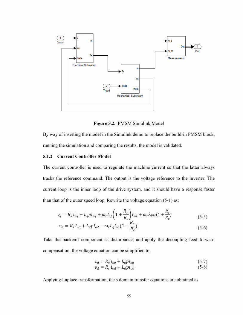
55
Figure 5.2. PMSM Simulink Model
By way of inserting the model in the Simulink demo to replace the build-in PMSM block,
running the simulation and comparing the results, the model is validated.
5.1.2 Current Controller Model
The current controller is used to regulate the machine current so that the latter always
tracks the reference command. The output is the voltage reference to the inverter. The
current loop is the inner loop of the drive system, and it should have a response faster
than that of the outer speed loop. Rewrite the voltage equation (5-1) as:
(
) 𝑀
(5-5)
(5-6)
Take the backemf component as disturbance, and apply the decoupling feed forward
compensation, the voltage equation can be simplified to
(5-7)
(5-8)
Applying Laplace transformation, the s domain transfer equations are obtained as

56
(5-9)
(5-10)
The PI current controller is used in this thesis works, as shown in Figure 5.3.
X PI Controller
PI ControllerX
X
X
id
id*+
-
+
-
iq
iq*
ud*+
+
W(1+Rs/Rc)(Ldid+lamda)
W(1+Rs/Rc)Lqiq
+
w
uq*
-
Figure 5.3 : Current Controller
In order to tune the PI-controller, the d-axis current loop in Figure 5.4 is used.
X PI Controller
id
id*+
-
ud*Inverter Motor
Measurement
Figure 5.4: d-axis current loop for PI tuning
The transfer functions for PI-controller are represented as:
(5-11)
The power inverter can be modeled as:
(5-12)

57
The motor plant transfer function is:
(5-13)
For the measurement feedback, it can be modeled as:
(5-14)
By rearranging the current loop, unity feedback can be achieved, as shown in Figure 5.5.
X PI Controller
id
id* +
-
ud*Inverter Motor MeasurementPrefilter
Figure 5.5: Unity feedback current loop
The pre-filter is used with transfer function
Thus, the open loop transfer function then can be obtained as:
(5-15)
Generally, the time constants for inverter and measurement are set to 50% of the
switching frequency of the inverter, as 0.5 . Compared with machine time constant,
they are much smaller, and can be approximated as one, first-order transfer function, with
time constant equal to the sum of each of them. Also, by applying pole-zero cancellation,
the slowest pole of the PMSM can be cancelled by the PI-controller. As a result, equation
(5-15) becomes:
(5-16)
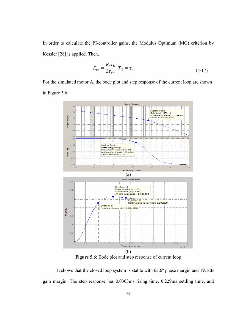
58
In order to calculate the PI-controller gains, the Modulus Optimum (MO) criterion by
Kessler [28] is applied. Then,
(5-17)
For the simulated motor A, the bode plot and step response of the current loop are shown
in Figure 5.6.
(a)
(b)
Figure 5.6: Bode plot and step response of current loop
It shows that the closed loop system is stable with 63.6° phase margin and 19.1dB
gain margin. The step response has 0.0303ms rising time, 0.229ms settling time, and

59
4.56% overshoot. The q-axis current controller can be tuned in the similar way as d-axis
current loop.
5.1.3 Speed Controller Model
Compared with the inner current loop, the speed loop is slower. In this thesis, the speed
loop is used to produce the torque command to the control strategy block. From
mechanical torque speed equation:
(5-18)
Take the load torque as disturbance, and neglect the friction viscous. The transfer
function of motor can be represented as:
(5-19)
where is torque constant.
The controller design is based on the speed loop shown in Figure 5.7.
X PI Controller
w
w* +
-
Te*Current
LoopMotor MeasurementPrefilter
Kt
Figure 5.7: Speed loop with unity feedback
Since the current loop is generally 10 times faster than the speed loop, it can be
approximated as a first order transfer function
(5-20)
The measurement transfer function is
(5-21)

60
The open loop transfer function then can be obtained as
(5-22)
In order to simplify the transfer function, the delays caused by the current loop and the
measurement can be approximated to a first order transfer function with time constant
as the sum of the delays. Then the open loop transfer function (5-22) becomes
(5-23)
Applying the Optimum Symmetric Method (OSM) [29], the optimal controller gain can
be calculated as
(5-24)
For simulation motor A, the bode plot and step response of the speed loop are shown in
Figure 5.7.
(a)

61
(b)
Figure 5.8: Bode plot and step response of current loop
The results show that the speed loop response is slower than that of the current
loop. And it is noted that the step response has a large overshoot. In order to avoid the
saturation of the controller output, the anti-windup technique can be used [30].
5.2 Machine Model Validation
A drive system has been built in Simulink using the PMSM model incorporated with core
loss. It is shown in Figure 5.9.
Figure 5.9: PMSM drive system in Simulink

62
The whole system includes current controller, speed controller and space vector
PWM blocks. The LMC and MTPA blocks are used to generate the dq-axis current
reference.
To validate the machine model, the simulation is carried out on Motor A first at
different operating conditions mentioned in following sections.
5.2.1 No-load Test Case Simulation
The speed response is investigated with zero d-axis current, at no load. At t = 0, the rated
speed command 188 rad/s is applied. And at t = 2.5s, the speed decreases to 120rad/s.
The results are presented in Figure 5.10.
(a) speed response (b) d-q-axis current
(c) phase current (d) d-q-axis voltage
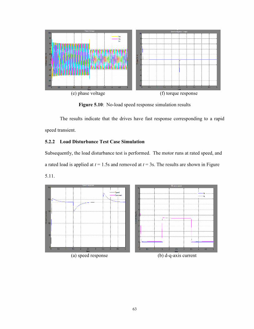
63
(e) phase voltage (f) torque response
Figure 5.10: No-load speed response simulation results
The results indicate that the drives have fast response corresponding to a rapid
speed transient.
5.2.2 Load Disturbance Test Case Simulation
Subsequently, the load disturbance test is performed. The motor runs at rated speed, and
a rated load is applied at t = 1.5s and removed at t = 3s. The results are shown in Figure
5.11.
(a) speed response (b) d-q-axis current

64
(c) phase current (d) d-q-axis voltage
(e) phase voltage (f) torque response
Figure 5.11: Load disturbance response simulation results
As the results indicate, the torque increases quickly to a high value when the load
is applied. It can also be seen that the q-axis current respond quickly to the rated current,
which can support the rated speed and load condition. Also, the phase voltage has the
same response as the current. The speed overshoot is a little bit large when the rated load
is applied and removed. This can be improved by weakening the integrating gain in the PI
speed controller.
5.2.3 Effect of d-axis Current on Loss Simulation
In order to investigate the effect of the d-axis current on the losses, a simulation is
conducted by applying a continuously changing d-axis current at the rated speed and the
rated load. Here, a ramp block in Simulink is used as d-axis current command. The slope

65
of the ramp signal is set as negative, and the initial value is set as zero. In other words,
the d-axis current is decreased from zero to the negative set value. The simulation results
are shown in Figure 5-12.
(a) d-q-axis current (b) torque response
(c) losses (d) efficiency
Figure 5.12. Effect of the d-axis current on loss simulation
The simulation results show that total electrical loss is a function of the d-axis
current. By injecting different id, the drives regulate the q-axis current to ensure the
machine running at the command operating point. It can be seen that the varied
combinations of id and iq give losses at different levels as well as changing machine
efficiency. Based on this observation, the loss minimization control can be achieved by
appropriately adjusting the id.

66
5.3 LMC Simulation
In order to test the LMC control strategy, the simulation will be carried out in different
cases. First, the steady state operation performance is simulated. And then the transition
performance between LMC and FWC is investigated. Last, the drive cycle simulation is
undertaken.
5.3.1 Steady State Simulation
The steady state simulation is performed on Motor A. It runs at the rated speed and the
rated load. The simulation time is 4 sec with LMC being applied for the first 2 seconds
and MTPA for the rest of the time. The results are shown as Figure 5.13.
(a) speed response (b) torque response
(c) phase current (d) phase voltage

67
(e) d-q current (f) flux
(g) loss (h) efficiency
Figure 5.13: Steady state simulation for LMC
It can be seen from the simulation results that LMC have fast speed and torque
response. When LMC is applied to the motor, id goes to more negative than that of
MTPA, and the phase current is larger than MTPA. However, since the id reduces the
total machine flux, the phase voltage of LMC becomes lower than MTPA. The loss
results also show that the copper loss is larger than MTPA due to larger phase current.
The iron loss is inferior to the one of MTPA, however, and their difference is greater than
the difference in copper loss. The total loss is found to decrease, and then the efficiency is
improved. This steady state simulation validates that the LMC has better performance

68
than MTPA from the efficiency point of view, while the former maintains the same speed
and torque response as the latter.
5.3.2 Simulation for Operating Above Base Speed
When the machine operates at above base speed, the MTPA cannot be applied anymore.
The LMC still can be used unless the voltage constraint is reached. As shown in Figure
5.14, the motor B will operate at 6000 rpm with 20 Nm load, and there are many options
for this condition between point A to point D along constant torque curve. Generally, flux
weakening control will choose point A, LMC will take point B, and MTPV will use point
C. In this simulation, the performance of the three controls will be compared.
Figure 5.14: Operating point of FWC, LMC, and MTPV
In this simulation, Motor B operates above the base speed, and the performance of
LMC is compared with that of FWC and MTPV.
0
100
200
300
400
500
-500 -400 -300 -200 -100 0
Iq (
A)
Id (A)
Voltage and Current Constraints
Imax
2600rpm
6000rpm
MTPA
MTPV
Te=134Nm
Te=60Nm
wlmc
Te=20Nm
LMC_6000rpm
A B D C
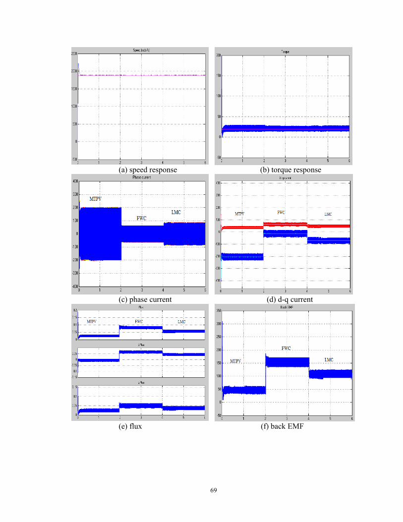
69
(a) speed response (b) torque response
(c) phase current (d) d-q current
(e) flux (f) back EMF

70
(g) losses (h) efficiency
Figure 5.15: Simulation comparison of MTPV, FWC, and LMC
The simulation results in Figure 5.15 show that MTPV, FWC and LMC all can
support the operating point above base speed. In term of losses, MTPV have minimized
core losses. LMC provides highest efficiency. The performance of FWC is between the
aforesaid two. It is noteworthy that for MTPV, the d-axis flux becomes a little bit
negative. As shown in Figure 5.14, the point C is located on the left side of the voltage
constraint center point (
, 0). Since in the simulation, Motor B has a
inferior to
the maximum phase current, it theoretically has an infinite extended speed range. It is
thus possible for the the d-axis flux to be negative. In real application, in order to avoid
the demagnetization of the permanent magnet, there are certain limiting factors for the
allowed maximum demagnetizing current.
5.3.3 Transition Simulation
This simulation is to test the performance of transition between LMC and FWC. The
speed is set to 6000 rpm, and the load rises from 0 to 60 Nm. Since the maximum
available torque of LMC for 6000 rpm is 38 Nm, the control should transfer from LMC
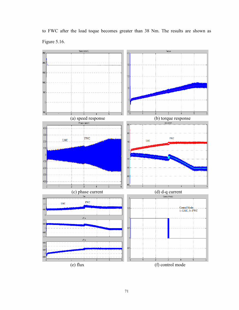
71
to FWC after the load toque becomes greater than 38 Nm. The results are shown as
Figure 5.16.
(a) speed response (b) torque response
(c) phase current (d) d-q current
(e) flux (f) control mode

72
(g) back EMF (h) efficiency
Figure 5.16: Transition simulation results
The simulation results in Figure 5.16 show that the speed and the torque have a
good tracking of the command. The transition from LMC to FWC happened at 3 second,
where the load torque rises to 36 Nm. After that point, the LMC current trajectory goes
outside the voltage constraint. So the control has to transfer to FWC. It is shown in back
emf result that the voltage goes up to around 173 V, which is the voltage constraint for
Motor B. In order to keep the machine working with voltage constraint, FWC forces the
current to more negative so as to weaken the flux. The flux result also shows that the
total flux decreases after FWC being applied until the machine reaches steady state. The
control mode plot is used to show the changes in control mode. It is consistent with the
simulation condition. During the transition, there is a short transient period as shown in
the dq current results.

73
Figure 5.17: Transition simulation current trajectory
By plotting the dq current simulation results in the dq current plane, it is observed
that the current exactly follows the LMC curve for 6000 rpm with load torque increasing.
After the maximum available torque is reached at the point A, the current trajectory is
going to follow the FWC’s current trajectory, which includes the intersection points
between the torque and voltage constraint curves. In other words, it is on the voltage
constraint eclipse.
5.3.4 Vehicle Drive Cycle Test Case Simulation
This test is to simulate one simple operating cycle of motor. The speed profile and load
torque profile are shown in Figure 5.18.

74
2 4 6 8 10 t (sec)
2600
6000
Speed (rpm)
A
B C
D F
G
H
2 4 6 8 10 t (sec)
60
134
Torque (Nm)
A
B
C D
E
E
F38
20G
H
Figure 5.18: Speed and torque profile of drive cycle
The machine starts up with large rated load 134 Nm, and speeds up to the rated
speed 2600 rpm. Once the speed is reached at 2 second, the load torque decreases
gradually to 60 Nm at 4 seconds. And then the machine speeds up again to 6000 rpm with
constant load torques 60 Nm. The machine stays at the 6000 rpm from 6 second, and the
load torque begins to reduce. At 8 second, the speed of the machine also decreases to zero
with load torque. The simulation results are shown as Figure 5.19.

75
(a) speed response (b) torque response
(c) phase current (d) d-q current
(g) efficiency (h) control mode
Figure 5.19: Drive cycle simulation results
It is observed that the cycle operation includes the steady state and the transition
between FWC and LMC. The speed and torque responses appear to be fast and stable
during the whole cycle. The current trajectory in dq current plane is plotted in Figure
5.20.

76
Figure 5.20: Drive cycle simulation current trajectory
When the simulation starts with the load torque 134 Nm, the speed goes up to the
rated value within 2 seconds. It is noted that the maximum available torque of LMC for
the rated speed is 133Nm. For speed less than the rated value, the LMC torque capacity is
higher, which can be seen from the torque speed envelop as described in Section 4.3.3.
Therefore, the control gives the command current following the intersect point of LMC
and torque curve even when the speed exceeds the critical speed . It is
corresponding to the region from point A to point B as shown in Figure 5.20. Since the
load torque is 1 Nm higher than the rate torque, there is a transition between LMC and
FWC around 2 second, which is shown in the simulation dq current and control mode
results. After the rated speed is reached, the load torque begins to decrease at 2 second.

77
Once the load torque goes down to less than the rated value, the control comes back to
LMC of the rated speed, and then the current should keep following the trajectory that is
the interval from point B to point C. At 4 second, the load torque stays at 60 Nm while
the speed goes up to 6000 rpm. During the rise of the speed, the transition occurs again at
5 second. From Figure 5.20, between point C and point D, the D’ represents the intersect
point of LMC for 4100 rpm with constant torque curve of 60 Nm, which means that the
maximum torque capacity for 4100 rpm LMC is 60 Nm. When speed goes over 4100
rpm, LMC cannot support this torque. So the control has to transfer to FWC. This
transition is also shown in the dq current and control mode results. At 6 second, the speed
stays at 6000 rpm, and the load torque decreases. Similar to the transition simulation in
Section 5.3.3, the 6000 rpm LMC can support the maximum 38 Nm torque. Before the
load torque decreases to less than 38 Nm, the control mode is still FWC. It is the region
from point D to point E. At 7 second, the load torque becomes less than 38 Nm, and the
control transfers back to LMC of 6000 rpm, which is region between point E and point F.
Finally, the speed and the load torque decrease together at 8 second, and reach zero at 10
second. The current trajectory follows the intersect point between LMC and torque curve,
for example, point G and point H at lower load and lower speed.
It can be seen that the simulation dq current result is exactly following the
trajectory of the proposed efficiency enhancement control algorithm. The result shows a
high average efficiency around 92.6% for the whole cycle operation.
5.4 Summary
In this chapter, the PMSM model with core loss resistance is built within the simulation
environment of Matlab/Simulink. With optimal design, the current and speed controllers

78
are also developed. The whole drive system for PMSM is finally implemented in the
Simulink. Two test machines are used to test the control strategies. The steady state
simulation is firstly performed with two cases, which include the operation below base
speed and that above base speed. The cases are corresponding to the current and voltage
constraint regions. The simulation results show that LMC can provide better efficiency if
compared with MTPA, MTPV and FWC. Also, the performance of the transition between
LMC and optimal FWC is investigated in voltage constraint region. Finally, a simple
drive cycle is simulated to test the proposed control strategy in a wide speed range with
load variation. Since the proposed control strategy is to generate the optimal current
trajectory for loss minimization of the machine, better efficiency can be achieved if the
drive system can track them properly. The simulation results suggest satisfactory tracking
performance of the drive system, while it still can maintain a good speed and torque
response.

79
CHAPTER 6 EXPERIMENTAL TESTS AND VERIFICATION
In this chapter, a laboratory designed surface mounted PMSM is used to test the proposed
algorithm. The simulation of this lab SPM is performed at first. Then the experimental
work is conducted by employing the efficiency enhancement control. The experimental
results are compared with simulation results and discussed in detail.
6.1 Simulation of SPM
The prototype SPM parameters are shown in Table 6.1.
Parameters Lab SPM
Rs (ohm) 0.1718
Rc (ohm) Measured
Ld (H) 3.36e-3
Lq (H) 3.36e-3
(V.s) 0.591
Vdc (V) 300
Pole number 4
Rated torque (Nm) 27
Power rating (hp) 5
Table 6-1: Prototype SPM Parameters
Before the simulation, the core loss resistance has to be identified. There are
different methods can obtained the core loss resistance [31,32]. In this research work,
based on the finite element analysis (FEA) results provided by the designer Maged, the
core loss resistance is calculated. Table 4 shows the calculation results. The core loss
resistance with respect to speed is also plotted in Figure 6.1. Using least square
algorithm, the expression of the core losses resistance is approximated as a linear
function of speed:

80
Speed
(Rpm)
Stator iron
loss
(W)
Rotor iron
loss
(W)
Totoal Iron
loss
(W)
BackEmf
(V)
Rc
(ohm)
200 2.133 0.00001361 2.13301361 30.77 443.8785279
400 4.55 0.00005428 4.55005428 61.53 831.8920897
600 7.253 0.0001215 7.2531215 92.3 1174.264645
800 10.24 0.0002146 10.2402146 123.1 1479.844727
1000 13.5 0.0003324 13.5003324 153.8 1750.88379
1200 17.05 0.0004738 17.0504738 184.6 1996.318688
1400 20.87 0.0006372 20.8706372 215.4 2219.959809
1600 24.96 0.0008213 24.9608213 246.1 2422.6084
1800 29.32 0.001024 29.321024 276.9 2609.721239
2000 33.95 0.001245 33.951245 307.7 2782.230091
Table 6-2: FEA results and core losses results
Figure 6.1: Core losses resistance
The simulations are performed on the lab SPM as illustrated in following sections.
0
500
1000
1500
2000
2500
3000
3500
0 100 200 300 400 500
Rc
(oh
m)
speed (rad/s)
Rc vs Speed

81
6.1.1 No-load Simulation
In this section, the no load simulation is performed by stepping up the speed of the lab
machine to1000 rpm. The loss performance of LMC and MTPA is investigated and
compared. The results are shown in Figure 6.2.
(a) speed response
(b) d-q current
(c) loss
Figure 6.2: No-load simulation of lab SPM
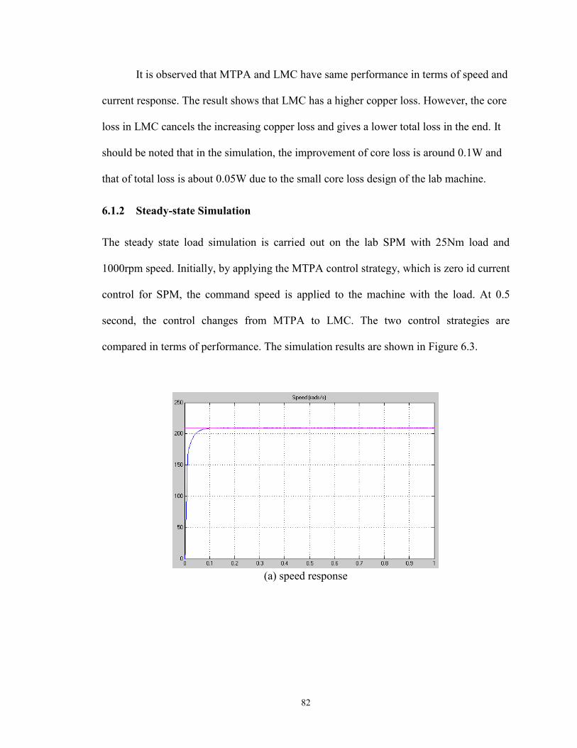
82
It is observed that MTPA and LMC have same performance in terms of speed and
current response. The result shows that LMC has a higher copper loss. However, the core
loss in LMC cancels the increasing copper loss and gives a lower total loss in the end. It
should be noted that in the simulation, the improvement of core loss is around 0.1W and
that of total loss is about 0.05W due to the small core loss design of the lab machine.
6.1.2 Steady-state Simulation
The steady state load simulation is carried out on the lab SPM with 25Nm load and
1000rpm speed. Initially, by applying the MTPA control strategy, which is zero id current
control for SPM, the command speed is applied to the machine with the load. At 0.5
second, the control changes from MTPA to LMC. The two control strategies are
compared in terms of performance. The simulation results are shown in Figure 6.3.
(a) speed response

83
(b) d-q current
(c) loss
Figure 6.3: 1000RPM with full load simulation of lab SPM
Since the torque of SPM is only related to q-axis current, the id variation does not
have any effect on the torque production. The results suggest that the id becomes a little
negative during LMC control, but maintains as zero for MTPA. There are no changes on
the torque and speed response as shown in the results. The flux becomes lower during
LMC due to negative id current, and then the core loss in LMC is lower than that in
MTPA. The result shows that MTPA has 153.4 W total loss, 138.51 W copper loss and
around 14.85 W core loss. When LMC is applied, the optimal id is around -0.3A. The

84
core loss decreases to 14.72 W, and copper loss goes up to 138.55 W. However, the core
loss in LMC cancels the increasing copper loss and gives a lower total loss in the end. It
should be noted that in the simulation, the improvement of core loss is around 0.13W and
that of total loss is about 0.1W. Also, it is observed that the optimal current for 1000rpm
without load and that with full load is the same. This can be explained by the solution of
LMC for SPM as shown in the equation (4-31), which is rewritten here:
Viewed from the equation, the optimal solution for SPM is not related to the q-axis
current. In other words, it is not related to the load.
Figure 6.4 shows 1600rpm and 2000 rpm with full load simulation results.
(a) 1600rpm speed response (b) 2000rpm speed response
(c) 1600rpm d-q current (d) 2000rpm d-q current

85
(e) 1600rpm loss (f) 2000rpm loss
Figure 6.4: 1600RPM and 2000RPM with full load simulation results
As shown in Figure 6.4, the optimal currents for the two high speed cases are -
0.54A and -0.62A respectively. It can be seen that the improvement of loss becomes
relatively larger than that in the 1000rpm case thanks to high speed with high core loss.
However, the improvement in itself is still small due to the small core loss design of the
lab machine, which gives around 0.2W and 0.4W loss improvement for 1600rpm and
2000rpm.
6.1.3 FEA Simulation and Verification
In order to validate the algorithm, the FEA experiments are also conducted on the lab
SPM with full load at three speeds. With gradually decreasing the d-axis current, the total
loss is recorded. The results are shown in Table 4:

86
Speed 1000RPM 1600RPM 2000RPM
id (A) Ptotal (W) Pcore (W) Ptotal (W) Pcore (W) Ptotal (W) Pcore (W) 0 153.3404915 14.8404915 165.581215 27.081215 175.091843 36.591843
-0.1 153.3004879 14.8004879 165.511206 27.011206 175.00183 36.50183
-0.15 153.2804862 14.7804862 165.481202 26.981202 174.951823 36.451823
-0.3 153.2204809 14.7204809 165.381189 26.881189 174.821803 36.321803
-0.6 153.7104711 14.6104711 165.383165 26.681165 174.661766 36.061766
-1 154.3604585 14.4604585 166.321134 26.421134 175.111719 35.711719
-1.5 155.8804443 14.2804443 167.691099 26.091099 176.871666 35.271666
-2 158.2004319 14.1004319 169.871068 25.771068 178.94162 34.84162
-2.5 161.2204207 13.9204207 172.75104 25.45104 181.721578 34.421578
-3 164.7304105 13.7304105 176.131015 25.131015 184.99154 33.99154
Improvement of loss compare to id=0
Loss
(W)
0.12 0.2 0.43
Table 6-3: FEA simulation results
Also, the results are plotted as Figure 6.5:
(a) 1000rpm FEA result
152
153
154
155
156
157
158
159
160
-4 -3 -2 -1 0
Loss
(W
)
id (A)
Totoal Losses for 1000rpm FEA

87
(b) 1600rpm FEA result
(c) 2000rpm FEA result
Figure 6.5: FEA total loss plot for 1000rpm, 1600rpm, and 2000rpm
The result for 1000rpm shows that the optimal d-axis current happens at around -
0.3A, and there is an around 0.12W improvement of loss compared to zero id. For
1600rpm, the optimal id is between -0.5A and -0.6A. For 2000rpm, the optimal id is
between -0.6A and -1A. The loss improvement is 0.2W and 0.43W respectively. This
result is consistent with the simulation result.
6.2 Experimental Testing and Verification
164
166
168
170
172
174
176
178
-4 -3 -2 -1 0
Loss
(W
)
id (A)
Total Losses for 1600rpm FEA
174
176
178
180
182
184
186
-3.5 -3 -2.5 -2 -1.5 -1 -0.5 0
Loss
(W
)
id (A)
Total Losses for 2000rpm FEA

88
6.2.1 Experimental Test Set-up
The setup of the experiment is shown in Figure 6.5, which includes power supply,
inverter, dSpace control system, lab SPM, and load system.
DCAC
PMSM Load
DC
Power
Supply
dSPACE System
Current
SensorEncoderMeasurement
Figure 6.6: Experiment setup block diagram
The dSPACE system provides a convenient environment to support model-based
control design and real time hard-in-loop (HIL) simulation. It can use the
Matlab/Simulink to develop the controller model, and the output signal will be sent to fire
the inverter. The feedback from encoder, current sensor and other measurements is sent
via the A/D port to the system. All the calculation and control processes are performed in
the Matlab/Simulink. The parameters of the experiment system are listed in Table 5.
Sampling time (sec) 2e-5
Switch frequency (KHz) 5
DC bus voltage (V) 250
Table 6-4: Experiment parameters

89
6.2.2 No-load Test
As observed from the simulation results, LMC gives the best optimal current in terms of
loss even though the improvement of the lab SPM is small. In order to capture the small
improvement of the loss, the experiment is at first performed with constant speed 800rpm
with no load. The id is swept from 0A to -5A with 0.2A step, and the input power is
recorded. Taking the average of the input powers for different ids so as to eliminate the
ripple, the results are plotted as Figure 6.9.
Figure 6.7: Input power result for varied id
The input power waveform of ids equal to -0.2A, -0.4A and -0.6A is shown in
Figure 6.10.
90
95
100
105
110
115
120
-5 -4 -3 -2 -1 0
po
we
r (W
)
id
Input Power vs Varied Id
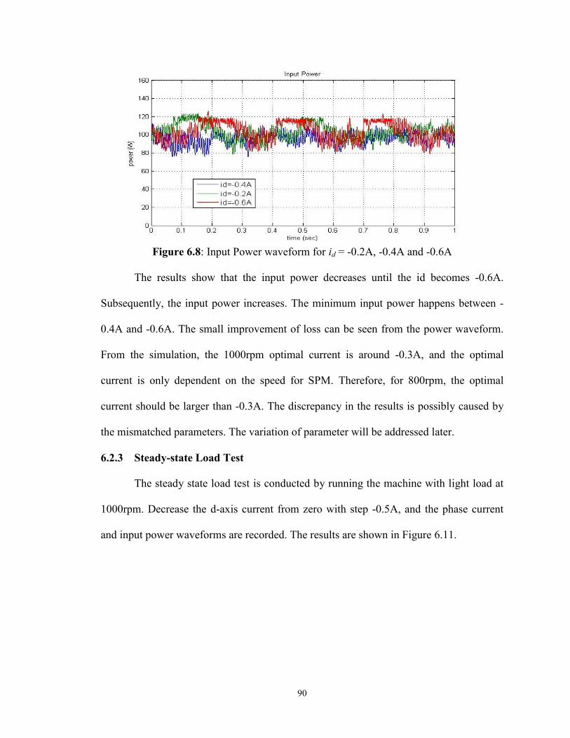
90
Figure 6.8: Input Power waveform for id = -0.2A, -0.4A and -0.6A
The results show that the input power decreases until the id becomes -0.6A.
Subsequently, the input power increases. The minimum input power happens between -
0.4A and -0.6A. The small improvement of loss can be seen from the power waveform.
From the simulation, the 1000rpm optimal current is around -0.3A, and the optimal
current is only dependent on the speed for SPM. Therefore, for 800rpm, the optimal
current should be larger than -0.3A. The discrepancy in the results is possibly caused by
the mismatched parameters. The variation of parameter will be addressed later.
6.2.3 Steady-state Load Test
The steady state load test is conducted by running the machine with light load at
1000rpm. Decrease the d-axis current from zero with step -0.5A, and the phase current
and input power waveforms are recorded. The results are shown in Figure 6.11.

91
(a) phase current
(b) input power
Figure 6.9: Steady-state load test results
The results show that the phase current increases with negative current injection.
The input power decreases a little bit when the id is -0.5A and increases at id equal to -
1A. The first three-step waveform captures the improvement of the input power even
though it is very small. The test suggests that the minimum power occurs at the point
around -0.5A. Compared with the simulation result -0.3A, a discrepancy also occurs with
same error direction with no load test. Despite that, the test proves that it is possible to
improve the total loss performance with certain negative id injection.
6.3 Discussion

92
The simulation results in Matlab/Simulink and FEA are essentially consistent. But they
both suggest that the improvement of the power is small even though LMC gives the best
efficiency optimal current. It is hard to capture the small improvement of the power due
to the design of the lab SPM. The experiment results do not show a significant
improvement of the power, and the optimal current point is not exactly matched with the
simulation. The discrepancy regarding the optimal current point is probably caused by
measurement errors or parameter mismatches. As a matter for fact, the model based LMC
is heavily dependent on the machine parameters. The optimal relationship between d-q
currents provides a generalized solution for efficiency enhancement, but it can be seen
that the hyperbolic equation’s coefficients include the machine parameters. The effect of
the parameter variation on LMC is analyzed later.
6.3.1 Effect of Core Loss Resistance
By varying the iron loss resistance from 60% to 140% of the nominal value, the copper
loss, iron loss, and total loss are plotted as Figure 6.12.
Figure 6.10. Effect of core loss resistance on the total loss
0
2000
4000
6000
8000
10000
12000
14000
-400 -350 -300 -250 -200 -150 -100 -50 0
Loss
es
(W)
D-axis current (A)
Ptotal, Pcu and Piron with varied Rc
Ptotal 0.6Rcnom Pcu 0.6RcnomPiron 0.6Rcnom Ptotal RcnomPcu Rcnom Piron RcnomPtotal 1.4Rcnom Pcu 1.4RcnomPiron 1.4Rcnom

93
It is observed that the copper loss Pcu is not affected much, but the iron loss Piron
has significant changes. And the total loss apparently shifts to the bottom right direction.
Also, the minimum total loss point as marked (*) in the plot shifts to the right. In other
words, the optimal point for the minimization of loss moves to the small negative d-axis
current. Plot the LMC in dq current plane as Figure 6.7.
Figure 6.11: LMC with variation of Rc
LMC moves to right with increasing Rc, which is consistent with the former
discussion. Also, for the experiment results, the total loss is larger than the simulation and
FEA results, which indicate that the real machine has smaller core losses resistance. This
probably explains why all the optimal currents are less than the simulation results. In
other words, the optimal current shifts to left due to small core loss resistance. The effect
of the stator resistance is plotted in Figure 6.14.
0
100
200
300
400
500
-500 -400 -300 -200 -100 0
Iq (
A)
Id (A)
Voltage and Current Constraints
LMC 0.6Rc
LMC Rc
LMC 1.4RcImax
2600rpm
Te=134Nm
Te=60Nm
Te=20Nm

94
Figure 6.12: LMC with variation of Rs
It shows that the stator resistance has similar effect on LMC as core loss
resistance. To be more exact, they both affect the copper loss instead of the core loss. The
optimal point of LMC moves to the right side of small negative d-axis current.
6.3.2 Effect of q-axis Inductance
In the PMSM, the inductance is not constant in fact. Instead, it is affected by cross
coupling and saturation issues. Especially, the q-axis inductance changes significantly
along with saturation. As a result, the variation of q-axis inductance also has impacts on
the total loss and the optimal loss points, which is plotted as Figure 6.9.
0
100
200
300
400
500
-500 -400 -300 -200 -100 0
Iq (
A)
Id (A)
Voltage and Current Constraints
LMC 0.6RsLMC RsLMC 1.4Rs
Imax
1667rpm
2600rpm
6000rpm
Te=134Nm
Te=60Nm
Te=20Nm

95
Figure 6.13. Effect of q-axis inductance on the total loss
The plot shows that the decrease of Lq will shift up the total loss curve and shift
the optimal loss point to left along the d-axis current, which means that the optimal point
for d-axis current will be of larger negative value. When the machine flux becomes
saturated, for the same load and the same speed, the current injected to the machine will
be larger than that in non-saturation condition. This explains why the copper loss and the
total loss have significant changes. Compared with general control strategy, LMC always
has negative d-axis current, which reduces the machine’s total flux. It helps to decrease
the saturation extent and then the variation of Lq.
Changes are observed for LMC trajectory in Figure 6.16, as well. LMC shifts to
right significantly when the Lq decreases to 60% of nominal value. For example, the
optimal point of 60Nm load with 2600 rpm moves from point A to point B.
0
2000
4000
6000
8000
10000
12000
14000
-400 -300 -200 -100 0
Loss
es
(W)
D-axis current (A)
Ptotal, Pcu and Piron with varied Lq
Ptotal 0.6Lqnorm Pcu 0.6LqnormPiron 0.6Lqnorm Ptotal LqnormPcu Lqnorm Piron LqnormPtotal 1.4Lqnorm Pcu 1.4LqnormPiron 1.4Lqnorm

96
Figure 6.14: LMC with variation of Lq
For the d-axis inductance, it is generally taken as constant in PMSMs when
compared to q-axis inductance. Its effect is plotted in Figure 6.17.
Figure 6.15: LMC with variation of Ld
It can be seen that LMC shifts to bottom left with the Ld decreasing from 140% to
60% of nominal value. The effect of Ld on LMC is not as much as that of Ld,
nevertheless.
0
100
200
300
400
500
-500 -400 -300 -200 -100 0
Iq (
A)
Id (A)
Voltage and Current Constraints
LMC 0.6LqLMC LqLMC 1.4Lq Imax
2600rpm with 0.6Lq
2600rpm with Lq
Te=134Nm
Te=60Nm
Te=20Nm
2600rpm with 1.4Lq
A
B
0
100
200
300
400
500
-500 -400 -300 -200 -100 0
Iq (
A)
Id (A)
Voltage and Current Constraints
LMC 0.6LdLMC LdLMC 1.4Ld Imax
2600rpm with 1.4Ld
2600rpm with Ld
Te=134Nm
Te=60Nm
Te=20Nm 2600rpm with 0.6Ld

97
6.3.3 Effect of Permanent Magnet Flux
The effect of permanent magnet flux linkage on LMC is plotted as Figure 6.18 and found
to be similar as that of the resistances. With the permanent magnet flux linkage
increasing, the optimal current trajectory shifts to the right side.
Figure 6.16: LMC with variation of PM flux
In real application, the PM flux linkage is affected mainly by the temperature,
which is similar to the resistance. The changes will be slower compared to the
inductance. With proper online parameter estimation techniques, the variation of machine
parameters can be compensated [33].
0
100
200
300
400
500
-500 -400 -300 -200 -100 0
Iq (
A)
Id (A)
Voltage and Current Constraints
LMC 0.6lamda
LMC lamda
LMC 1.4lamda
Imax
2600rpm with 0.6lamda
2600rpm wtih lamda
Te=134Nm
Te=60Nm
Te=20Nm
2600rpm with 1.4lamda
98
CHAPTER 7 CONCLUSIONS AND FUTURE WORK
7.1 Conclusions
As the energy and environmental issues contribute to the ever-growing interest in
EV/PHEV application, a lot of research has been conducted on the traction system of
EV/PHEV, which mainly includes power source, power electronics, and traction motor.
Since the sole power source for EV/PHEV application comes from the battery, the whole
system efficiency will be very important when the distance per charge is taken into
consideration. A lot of research has been focused on MTPA and MTPV, the two control
modes that achieve minimized copper loss and minimized core loss respectively. Also,
there have been a few studies considering both copper loss and core loss reduction in this
regard.
In this thesis, the working principles of PMSMs are examined closely. For control
purpose, the mathematic model of PMSMs is built by Park’s transformation, which
transfers a three phase model to a fiction two phase coordinate system. The model in the
two phase coordinate system is generally called dq model. With the rotor reference
frame being chosen, the time dependent variables such as the inductance in the three
phase model becomes constant, which significantly facilitates the control design. Based
on the dq model of PMSMs, the equivalent circuit is modeled to investigate the dynamic
and static performances of PMSMs. According to the power flow in the machine,
different losses are identified. As for core loss, it is modeled as a resistance component
that is a parallel branch in the equivalent circuit. Based on this equivalent circuit, the total
loss is formulated as a function of the d-axis current. The plot of the total loss function
indicates that it is a concave curve with respect to the d-axis current. This suggests a

99
possibility to control the machine with minimum loss. LMC is developed from this
consideration. An optimal current relationship is found to satisfy the loss minimization
need corresponding to the speed. The operating boundary region for LMC is analyzed
with the voltage constraint and the current constraint both being taken into account. For
the operation outside the LMC boundary region, an optimal FWC is employed, which can
provide a better loss performance. In so doing, the efficiency enhancement control
algorithm over full speed range is formed with the combined use of LMC and optimal
FWC. Also, the optimal current relationship is proved to be a generalized expression for
efficiency improvement algorithm. Control modes such as MTPA and MTPV, which can
be considered as special cases of LMC, can be derived from the generalized optimal
current trajectory.
A drive system is built in Matlab/Simulink environment for the purpose of
validating the control algorithm. Two testing machines with different power ratings are
used in the simulation work. The steady state test is performed with the machine
operating in both current constraint and voltage constraint regions. The simulation results
indicate that the proposed algorithm give better loss performance than MTPA and MTPV
without losing speed and toque responses. The transition simulation is also carried out to
test the performance of the control mode transition between LMC and optimal FWC.
Finally, the drive cycle simulation is conducted with a wide speed range and a load
variation profile, whose results show a good optimal current tracking performance.
Experimental test is also performed on a lab designed SPM. The experiment results show
a discrepancy from the simulation results, which might be caused by measurement errors

100
and mismatches of the machine parameters. Despite the discrepancy, the experiment
proves that with the proposed control algorithm, a reduction of the losses is possible.
7.2 Future Work
The simulation and experiment results prove the utility of the proposed algorithm as well
as raises the following questions that have to be tackled with in the future work:
The algorithm uses a resistance component to model the core loss. Therefore, an
accuracy measurement procedure of the core loss resistance should be developed.
The core loss characteristics have to be investigated in more detail, and there is a
need to develop a simple and accurate core loss model for the control purpose.
Since the algorithm is dependent on the machine parameters, proper estimation
techniques have to be developed for online parameters.
The proposed algorithm can be combined with search-based techniques to avoid
parameters dependency, which can provide the initial current reference to the
search method to accelerate the convergences.
The model based control algorithm does not include the inverter losses, which
should be added due to the cross effect between the inverter and the motor. For
example, LMC injects a negative d-axis current into the machine to improve the
efficiency of the machine. However, it increases the phase current, which means
that the inverter loss will increase.

101
REFERENCES
[1] Z.Rahman, M.Ehsani and K.L.Butler, “An investigation of Electric Motor Drive
Characteristics for EV and HEV Propulsion Systems”, SAE Technical Paper Series,
2000-01-3062.
[2] Williamson, S.S.; Emadi, A.; Rajashekara, K., "Comprehensive Efficiency Modeling
of Electric Traction Motor Drives for Hybrid Electric Vehicle Propulsion Applications,"
Vehicular Technology, IEEE Transactions on , vol.56, no.4, pp.1561,1572, July 2007
[3] M. Olszewski, “Final Report on Assessment of Motor Technologiesfor Traction
Drives of Hybrid and Electric Vehicles”, subcontract No. 4000080341, Oak Ridge
National Laboratory, March 2011.
[4] Uddin, M.N.; Radwan, T.S.; Azizur Rahman, M., "Performance of interior permanent
magnet motor drive over wide speed range," Energy Conversion, IEEE Transactions on ,
vol.17, no.1, pp.79,84, Mar 2002
[5] Inoue, Y.; Morimoto, S.; Sanada, M., "A Novel Control Scheme for Maximum Power
Operation of Synchronous Reluctance Motors Including Maximum Torque Per Flux
Control," Industry Applications, IEEE Transactions on , vol.47, no.1, pp.115,121, Jan.-
Feb. 2011
[6] Mademlis, C.; Margaris, N., "Loss minimization in vector-controlled interior
permanent-magnet synchronous motor drives," Industrial Electronics, IEEE Transactions
on , vol.49, no.6, pp.1344,1347, Dec 2002
[7] Bazzi, A.M.; Krein, P.T., "Comparative evaluation of machines for electric and
hybrid vehicles based on dynamic operation and loss minimization," Energy Conversion
Congress and Exposition (ECCE), 2010 IEEE , vol., no., pp.3345,3351, 12-16 Sept. 2010

102
[8] Fernandez-Bernal, F.; Garcia-Cerrada, A.; Faure, R., "Model-based loss minimization
for DC and AC vector-controlled motors including core saturation," Industry
Applications, IEEE Transactions on , vol.36, no.3, pp.755,763, May/Jun 2000
[9] Krishna, R., “Permanent Magnet Synchronous and Brushless DC Motor Drives,”
CRC Press, Taylor & Francis Group, LLC, 2010
[10] Krishna, R., Electric Motor Drives, Prentice Hall, Upper Saddle River, NJ, 2001
[11] S.Morimoto, Y.Takeda, T.Hirasa, K. Taniguchi, “Expansion of Operating Limmits
for Permanent Magnet Motor by Current Vector Control Considering Inverter Capacity,”
IEEE Trans, on Ind, Appl., Vol. 26, No. 5, 1990.
[12] W.L. Soong and T.J.E. Miller, “Field-weakening performance of brushless
synchronous AC motor drives”, IEEE Proc-Electr. Power Appl., Vol. 141, No. 6,
November 1994.
[13] F.Blaaske, “The principle of field orientation as applied to the new transvector
closed-loop control system for rotating field machine”, Siemens Review, Vol.34, pp.217-
220,1972
[14] Pillay, P., "Vector control of AC permanent magnet machines," Electrical Machines
and Drives, 1989. Fourth International Conference , pp.293,297, 13-15 Sep 1989
[15] Takahashi, I.; Noguchi, T., "A New Quick-Response and High-Efficiency Control
Strategy of an Induction Motor," Industry Applications, IEEE Transactions on , vol.IA-
22, no.5, pp.820,827, Sept. 1986

103
[16]K.T. Chau, C.C. Chan, Chunhua Liu, "Overview of Permanent-Magnet Brushless
Drives for Electric and Hybrid Electric Vehicles," IEEE Trans. on Industrial Electronics,
vol. 55, no. 6, pp. 2246-2257, June 2008.
[17] Ching-Tsai Pan; Shinn-Ming Sue, "A linear maximum torque per ampere control for
IPMSM drives over full-speed range," Energy Conversion, IEEE Transactions on ,
vol.20, no.2, pp.359,366, June 2005
[18] Morimoto, S.; Sanada, M.; Takeda, Y., "Wide-speed operation of interior permanent
magnet synchronous motors with high-performance current regulator," Industry
Applications, IEEE Transactions on , vol.30, no.4, pp.920,926, Jul/Aug 1994
[19] Roy S.Colby, Donald W. Novotny, “An efficiency-Optimizing Permanent Magnet
Synchronous Motor Drives,” IEEE Transaction on Industry Application, Vol. 24, No. 3,
pp. 462-469, May, 1988.
[20] S.Morimoto, Y.Tong, Y. Takeda, and T. Hirasa, “Loss minimization control of
permanent magnet synchrounou motor drives,” IEEE Trans. Ind. Electron.,Vol. 41, no. 5,
pp. 511-517, Oct. 1994
[21] C.C.Chan and K.T.Chau, “An advanced permanent magnet motor drive system for
battery-powered electric vehicles,” IEEE Trans. Veh. Technol.,vol. 45, no. 1, pp.180-188,
Feb, 1996.
[22] Sadegh Vaez-Zadeh,V.I. John, M.A.Rahman, “An on-line loss minimization
controller for interior permanent magnet motor drives,” IEEE Trans. on Energy
Conversion, Vol. 14, No. 4, pp. 1435-1440, Dec.1999.

104
[23] C.Cavallaro, A.O.D. Tommaso, R.Miceli, A. Raciti, G.R. Galluzzo, and
M.Tranpanese, “Efficiency enhancement of permanent-Magnet Synchronous Motor
Drives by Online Loss Minimization Approaches,” IEEE Trans. Ind. Electron.,Vol. 52,
no. 4, pp.1153-1160, Aug. 2005
[24] J. G. Lee, K. H. Nam, S. H. Lee, S. H. Choi, and S. W.Kwon, "A lookup table based
loss minimizing control for FCEV permanent magnet synchronous motors,"Journal of
Electrical Engineering & Technology, Vol. 4, No. 2, pp. 201-210, Jun. 2009.
[25] Junggi Lee, Kwanghee Nam, Seoho Choi, Soonwoo Kwon, “Loss Minimizing
Control of PMSM with the Use of Polynomial Approximations,” Industry Applications
Society Annual Meeting, 2008. IAS '08. IEEE , pp: 1 – 9, Oct. 2008.
[26] E. S. Sergaki, P. S. Georgilakis, A. G. Kladas, G. S. Stavrakakis, Fuzzy Logic Based
Online Electromagnetic Loss Minimization of Permanent Magnet Synchronous Motor
Drives, Proceedings of the 2008 Int. Conference on Electrical Machines, ICEM 2008,
Vilamoura, Portugal, Sep. 2008.
[27] Eleftheria S. Sergaki, Nikolaos M. Afentakis, George S. Stavrakakis, An Hybrid
Loss Minimization Controller incorporated into ACIM speed FOC motor drive, based on
a General Loss Model and on a Fuzzy Logic Search Controller, for Transient and Steady
States, Proceedings of The World 2009 Congress on Power and Energy Engineering,
(WCPEE’09), Cairo, Egypt, Oct.5-8, 2009.C
[28] Preitl, Z.; Bauer, P.; Bokor, J., "A Simple Control Solution for Traction Motor Used
in Hybrid Vehicles," Applied Computational Intelligence and Informatics, 2007. SACI
'07. 4th International Symposium on , vol., no., pp.157,162, Yearly 17 2007-May 18 2007

105
[29] Umland, J.W.; Safiuddin, M., "Magnitude and symmetric optimum criterion for the
design of linear control systems: what is it and how does it compare with the others?,"
Industry Applications, IEEE Transactions on , vol.26, no.3, pp.489,497, May/Jun 1990
[30] Pillay, P.; Krishnan, R., "Control characteristics and speed controller design for a
high performance permanent magnet synchronous motor drive," Power Electronics, IEEE
Transactions on , vol.5, no.2, pp.151,159, Apr 1990
[31] Urasaki, N.; Senjyu, T.; Uezato, K., "A novel calculation method for iron loss
resistance suitable in modeling permanent-magnet synchronous motors," Energy
Conversion, IEEE Transactions on , vol.18, no.1, pp.41,47, Mar 2003
[32] Yamazaki, K.; Seto, Y., "Iron loss analysis of interior permanent-magnet
synchronous motors-variation of main loss factors due to driving condition," Industry
Applications, IEEE Transactions on , vol.42, no.4, pp.1045,1052, July-Aug. 2006
[33] L. Kan, Q. Zhang, J. Shen, S. Paul, “Comparison of two novel MRAS strategies for
identifying parameters in permanent magnet synchronous motors,” International Journal
of Automation and Computing, Vol. 3, 2010, pp. 516- 524.