ORIGINAL PAPER

Loss in moment capacity of tree stems induced by decay

Cihan Ciftci • Brian Kane • Sergio F. Brena •

Sanjay R. Arwade

Received: 7 August 2013 / Revised: 23 November 2013 / Accepted: 12 December 2013 / Published online: 29 December 2013

� Springer-Verlag Berlin Heidelberg 2013

Abstract

Key message We model varying decay in tree cross-

sections by considering bending theory to estimate

moment capacity loss (MCL) for the sections. We

compare MCL with experiments on selected oak trees.

Abstract Tree failures can damage property and injure

people, sometimes with fatal consequences. Arborists

assess the likelihood of failure by examining many factors,

including strength loss in the stem or branch due to decay.

Current methods for assessing strength loss due to decay

are limited by not accounting for offset areas of decay and

assuming that the neutral axis of the cross-section corre-

sponds to the centroidal axis. This paper considers that

strength loss of a tree can be related to moment capacity

loss (MCL) of the decayed tree cross-section, because tree

failures are assumed to occur when induced moments

exceed the moment capacity of the tree cross-section. An

estimation of MCL is theoretically derived to account for

offset areas of decay and for differences in properties of

wood under compressive and tensile stresses. Field mea-

surements are used to validate the theoretical approach, and

predictions of loss in moment capacity are plotted for a

range of scenarios of decayed stems or branches. Results

show that the location and size of decay in the cross-section

and relative to the direction of sway are important to

determine MCL. The effect of wood properties on MCL

was most evident for concentric decay and decreased as the

location of decay moved to the periphery of the stem. The

effect of the ratio of tensile to compressive moduli of

elasticity on calculations of MCL was negligible. Practi-

tioners are cautioned against using certain existing methods

because the degree to which they over- or underestimate

the likelihood of failure depended on the amount and

location of decay in the cross-section.

Keywords Tree decay � Strength loss � Oscillation �Oak � Wind � Winching

Introduction

Tree risk assessment is an important aspect of arboricul-

tural practice. Tree failures regularly damage property and

injure people. From 1995 to 2007, 407 people died in the

US as a result of wind-related tree failures (Schmidlin

2009), although the presence of defects prior to tree failure

was not assessed. There is also a risk of litigation associ-

ated with tree failures (Mortimer and Kane 2004), so the

economic cost may be much greater than the direct cost of

tree and debris removal and associated damage repair.

Examples can be found in most cities: a recent series of

articles in the New York Times detailed multiple lawsuits

stemming from fatalities and injuries associated with haz-

ardous trees (Glaberson and Foderado 2012).

The risk of tree failure due to decay may be quantified

through different techniques that range from simple visual

inspection (Fink 2009) to sophisticated decay detection

Communicated by T. Fourcaud.

C. Ciftci (&)

Department of Civil Engineering, Abdullah Gul University,

Kayseri, Turkey

e-mail: cihan.ciftci@agu.edu.tr

B. Kane

Department of Environmental Conservation, University of

Massachusetts, Amherst, MA, USA

S. F. Brena � S. R. Arwade

Department of Civil and Environmental Engineering, University

of Massachusetts, Amherst, MA, USA

123

Trees (2014) 28:517–529

DOI 10.1007/s00468-013-0968-8

methods involving tomography (Gilbert and Smiley 2004;

Nicolotti et al. 2003; Wang and Allison 2008), radar

(Butnor et al. 2009), or tree performance measurements

using strain gages and inclinometers (Sinn and Wessolly

1989). Assessing decay has been the focus of much

research, primarily in the form of decay detection devices

(Johnstone et al. 2010). Quantifying the amount of decay

has been related to the probability of failure using strength

loss formulas (Coder 1989; Mattheck et al. 1993; Smiley

and Fraedrich 1992; Wagener 1963). Kane et al. (2001)

reviewed the formulas and found that all are based on the

moment of inertia (I) of a circular cross-section [excepting

Mattheck et al. (1993)], and have been calibrated using

empirical evidence. It should be noted that the level of

sophistication and the quantity of investigations of testing

of devices to detect decay far exceed the sophistication,

accuracy and quantity of investigations of the strength loss

formulas.

Wagener (1963) determined strength loss of a stem by

dividing the cube of diameter of a, presumed, circular area

of decay by the cube of the stem diameter (also assumed to

be circular). This is a more conservative estimate of the

loss in I of a circular cross-section due to a concentric,

circular area of decay, which was Coder’s (1989) approach.

He estimated strength loss as the ratio of the diameter of a

circular area of decay raised to the fourth power and the

stem diameter raised to the fourth power. Wagener (1963)

used a more conservative estimate of the loss in I given the

limitations of the procedure. Limitations include: (1) nei-

ther stem cross-sections nor areas of decay are always

perfectly circular; (2) bark thickness is not considered; (3)

trees are not equivalent to defect-free specimens used to

determine wood properties—slope of grain, reaction wood,

juvenile wood, and branches (knots) are part of the tree;

and (4) genetics and growing conditions contribute to

variation in wood properties among individuals of a

species.

Despite Wagener’s (1963) more conservative assess-

ment of the loss in I, additional limitations undermine the

accuracy of the formulas. Primary among these is that the

formulas do not explicitly consider the location of decay

relative to the neutral axis and the distance between the

neutral axis and the location of the maximum bending-

induced normal stress (r). The latter is related to the

applied moment using the flexure formula for elastic

materials that remain below the proportional limit:

r ¼ Mc=I ð1Þ

where M is the bending moment and c is the maximum

perpendicular distance from the neutral axis to the outer

surface of the branch or stem. Non-concentric areas of

decay reduced the accuracy of Wagener’s (1963) and

Coder’s (1989) formulas to predict strength loss (Kane and

Ryan 2004) and breaking strength (Ruel et al. 2010) of

stems. Stresses associated with axial forces are typically

ignored when investigating strength loss because their

magnitude is small as compared to bending stress (Matt-

heck et al. 1994).

A second limitation of the strength loss formulas is that

they assume a homogeneous and isotropic material where

tensile and compressive stresses depend on the same

modulus of elasticity. Although conventional sources usu-

ally provide a single value for the modulus of elasticity

(E) of wood in bending (e.g., Kretschmann 2010), some

work has shown that E is greater in tension (ET) than in

compression (EC) (Langum et al. 2009; Langwig et al.

1968; Ozyhar et al. 2013; Schneider et al. 1990). Conse-

quently, the strain and stress distributions, under the clas-

sical assumptions of beam theory, will not be proportional

to one another. Since E applies only to strains in the elastic

range well below yield stress, an alternative value of

E could be determined as the secant of a stress–strain curve

including the non-linear region of plastic strains preceding

rupture. Since wood is stronger in tension than compres-

sion (Bodig and Jayne 1993), in the region of non-linear

strains, E determined from the secant would reflect dif-

ference between tensile and compressive values.

Finally, none of the formulas considers growth stresses,

which are tensile at the periphery of the stem and com-

pressive at the pith. Growth stresses can vary greatly

among individuals of a given species (Jullien et al. 2013)

and are greater on leaning stems due to the presence of

reaction wood (Okuyama et al. 1994; Wilson and Gartner

1996; Yoshida et al. 2002). Depending on the particular

conditions, the effect of growth stress may supersede any

effect due to differences in ET and EC.

The objective of this paper is to improve predictions of

MCL that account for areas of decay that vary with respect

to size and distance from the perimeter of the cross-section,

as well as those of irregular shapes. A secondary objective

is to investigate whether the magnitude of disparity

between the tensile and compressive elastic moduli of

wood affected the reliability of the predictions.

Materials and methods

In deriving the improved predictions of MCL, several

assumptions have been made. First, it was assumed that the

stem or branch is subjected to pure bending stress; the

effects of axial, shear and torsional stresses have been

ignored. The reasons for this assumption were that wind-

induced tree failures typically involve bending stress due to

tree sway (James 2003) and experimental verification of

the improved predictions involved primarily bending

stress. Second, cross-sectional areas of the stem and decay

518 Trees (2014) 28:517–529

123

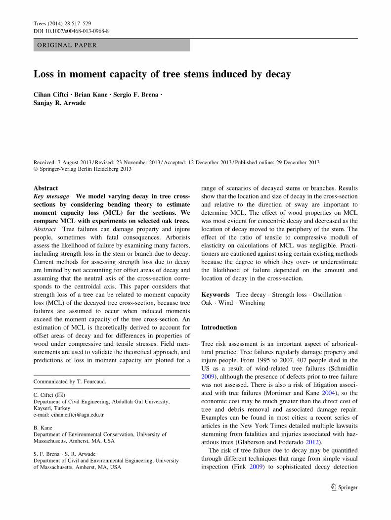
were assumed to be circular and defined by radii R and r,

respectively, as shown in Fig. 1. The area of decay, still

considered to be circular for simplicity, can also have an

open cavity as in the right-hand side of Fig. 1. Third, the

derivation assumes that the bending moment is applied on

the plane whose intersection with the cross-section defines

the line along a diameter that passes through the center of

both the area of decay and the cross-section of the stem

(Fig. 1). This assumption results in the maximum MCL of

the cross-section, reflecting the greatest increase in likeli-

hood of failure. Fourth, it has been assumed that:

(a) ET [ (EC) (Langum et al. 2009), and (b) moment

capacity is governed by compressive yield stress (Bodig

and Jayne 1993), which is one-half that of tensile yield

stress (Mattheck et al. 1994) and therefore defines the

initiation of the failure process even though final apparent

failure of the stem will manifest as tensile fracture. Lastly,

the effect of growth stresses has been ignored. Previous

studies have shown axial tensile growth stress in oaks of

about 6 MPa (Okuyama et al. 1994; Wilhelmy and Kubler

1973; Yao 1979).

Definition of circular decay in tree cross-sections

The distance, r0 in Fig. 1 defines the distance parallel to the

diameter between the centers of the circular areas repre-

senting decay and the stem (Fig. 1). The ratio r0/R will be

used to evaluate the effect of decay position on MCL.

Theoretical approach and implementation

Moment capacity of the stem cross-section (with and

without decay) can be calculated as the total moment of

compressive and tensile stress resultants about the neutral

axis of the cross-section. Thus, the first step in calculating

moment capacity of stems with and without decay is to

determine the location of the neutral axis. Figure 2 shows a

representative stem cross-section with decay, as well as

distributions of compressive and tensile strains and stresses

(including the resultant compressive (FC) and tensile (FT)

forces induced by bending). By definition, the neutral axis

is located where bending strains are zero; it defines the

transition between compressive (eC) and tensile (eT) strains.

Because the section is subjected to pure bending, axial

force equilibrium requires that FC = FT.

The location of the neutral axis coincides with the

centroidal axis of the cross-section of the stem only for a

section made from a homogeneous material that has sym-

metrical stress–strain response for both tension (ET) and

compression (EC). That is, when

n ¼ ET=EC ¼ 1 ð2Þ

By defining the modular ratio n and transforming the

cross-section to an equivalent homogeneous material, the

neutral axis can be determined following basic principles

of strength of materials. The main difficulty lies in an

accurate determination of ET and EC. Such values are

sparse in the literature (Langum et al. 2009), and vary by

species and growing conditions (Bodig and Jayne 1993).

Schneider and Phillips (1991) note that there is no reason to

expect that ET and EC should be equal. If n = 1, MCL can

be determined analytically for areas of decay located

entirely within the cross-section of a stem (‘‘Appendix B’’).

The effect of the location of the neutral axis on MCL

was investigated by using two different values of n (1.1 and

2.0). For n [ 1.0, the neutral axis will be closer to the

R

r

r0

Tension Side

Compression Side

R

r

Tension Side

Compression Side

NA

r0

NAFig. 1 Decay definition in tree

cross-sections. The circle of

radius r, outlined with a dashed

line, indicates an area of decay.

The left-hand figure is an

example for a cavity completely

contained within the tree cross-

section and the right-hand figure

is an example of a cavity that

has breached the perimeter of

the cross-section. The neutral

axis, NA (where there are no

bending strains) is the dashed

straight line that separates the

tension and the compression

sides of the cross-sections. All

symbols are explained in

‘‘Appendix A’’

Trees (2014) 28:517–529 519

123

tension side of the cross-section, so greater strains are

generated on the compressive side where FC acts. (Langum

et al. 2009) presented values for young Douglas-fir

(Pseudotsuga menziesii (Mirb.) Franco) and western hem-

lock (Tsuga heterophylla (Raf.) Sarg.); the mean value of

n was approximately 1.1 (EC = 9,750 MPa and

ET = 10,400 MPa). To determine whether the value of

n affected MCL, n = 2.0 was also tested. These values

covered the range of previously reported values of n (Lan-

gum et al. 2009; Langwig et al. 1968; Ozyhar et al. 2013;

Schneider et al. 1990). Figure 2 shows that n dictates the

proportional disparity between similar triangles represent-

ing eT and eC. For a given strain distribution, a stress dis-

tribution can be calculated (Fig. 2). The neutral axis was

initially assumed to be at 1 % of the diameter of the cross-

section, an unrealistically small value. Tensile and com-

pressive strains that resulted from the assumed position of

the neutral axis at each value of n were used to calculate rC

and rT using Hooke’s Law, assuming linear behavior of the

material:

ri ¼ Eiei ð3Þ

where i designates compressive or tensile values of each

parameter. From the distributions of compressive (rC) and

tensile (rT) stresses, the resultant forces (FC and FT) were

calculated by integrating rC and rT over the cross-sectional

areas (Fig. 2). For each value of n, the preceding steps were

repeated after gradually increasing the distance between

the neutral axis and outer tension face of the stem in Fig. 1

until force equilibrium (FC = FT) was satisfied.

Once the location of the neutral axis of the tree cross-

sections with and without decay was known, the moments

of FC and FT about the neutral axis were calculated.

Moment capacity of each section was defined as the total

moment that generated a compressive stress in the extreme

fiber equal to the compressive yield stress [taken from

Kretschmann (2010)]. MCL due to decay was calculated:

MCL ¼ 1 � MCd

MCud

ð4Þ

where MCd and MCud are the moment capacities of the

decayed and un-decayed sections, respectively.

Experiments on MCL

To validate the predictions of MCL for different amounts

and locations of decay, ten red oaks (Quercus rubra L.)

growing in Pelham, MA, USA (USDA Hardiness Zone 5A)

were tested. Morphometric data of the trees are presented

in Table 1. A static pull test similar to those summarized

by (Peltola 2006) was used to test the trees. To limit the

effect of the offset mass of the crown during testing,

branches were removed prior to testing. A snatch block

(McKissick Light Champion model 419) was attached to

the tree with an Ultrex sling (1.9 cm diameter, Yale

Cordage, Saco, ME) at approximately 65 % of its height.

Trees were pulled using a skidder (John Deere model

440D) with a hydraulic winch and 61 m of Vectrus (1.3 cm

diameter, Yale Cordage, Saco, ME). The rope was passed

εt

ε c

NA NA

FT

FC

σc - yield

σt

StressesStrainsCross-Section

Compression Side

Tension Side

Fig. 2 Strains and stresses in compression and tension sides of tree

cross-sections. The neutral axis, NA (where there are no bending

strains) is the dashed straight line that separates the tension and the

compression sides of the cross-sections. Axial stress due to self-

weight and growth stresses have been ignored. All symbols are

explained in ‘‘Appendix A’’

Table 1 Morphometric data for ten red oaks tested to validate the-

oretical calculations of moment capacity loss

Parameter Mean SD

DBH (cm) 41 4.3

Tree height (m) 21.6 1.2

Crown width (m)a 11.9 2.3

Height of block (m) 13.8 1.3

Height of first branch (m) 10.3 2.1

Stem diameter at block (cm) 18 1.8

Angle between cable and tree (�) 73 2.5

% Of diameter notched (Type 1) 40 8.0

% Of diameter notched (Type 2) 12 6.0

a Calculated as the mean of widths measured parallel and normal to

the direction of applied load

520 Trees (2014) 28:517–529

123

through the block and attached to a load cell (Dillon

EDXtreme, Weigh-Tronix, Fairmont, MN) that recorded

loads (accurate to 44 N) at 10 Hz. Loads were doubled,

which was an overestimate because there was some amount

of friction in the block, but this was assumed to be minor.

Loads were resolved into components parallel and normal

to the long axis of the trunk. Taking the sine of the mean

angle between the applied force and the tree (Table 1)

indicated that 96 % of the load was applied normal to the

long axis of the trunk and induced a bending moment.

A strain meter was attached to the tension side of the

stem approximately 1 m above ground as described by

James and Kane (2008), which recorded axial displace-

ments, which were converted to strains, at 20 Hz. To relate

displacements with loads, the mean of two displacements

was related with a single load for each 0.1 s. Trees were

winched to induce axial displacements at the height of the

strain meter of approximately 1–2 mm to ensure that

induced stresses remained in the elastic range. The rate of

loading varied with trees of different dimensions and time

in the test (initial rates were less). Loading rate ranged

from approximately 100–200 N/s, which induced dis-

placements at a rate of approximately 0.1–0.2 mm/s.

After winching, a notch with its longitudinal axis normal

to the direction of winching and the longitudinal axis of the

trunk was cut into each tree with a chainsaw. Two types of

notches were cut: (1) into the tension face of the trunk,

removing all of the wood on the perimeter of the stem (two

tests); (2) through the tree leaving wood intact at the

perimeter of the trunk on the tension and compression faces

(eight tests) (Fig. 3). More Type 2 notches were cut

because of the variability of the location of the notch rel-

ative to the center of the trunk (as measured incident with

the applied load). Three Type 2 notches left approximately

equal thicknesses of wood on the proximal and distal sides

of the trunk (relative to the position of the skidder); two left

a greater thickness of wood on the proximal side of the

trunk; and five left a greater thickness of wood on the distal

side of the trunk. The mean percent of trunk diameter

removed for each type of notch is included in Table 1.

Bending force was plotted against strain before and after

the notch was cut on each tree. The slopes of the best-fit

lines in Fig. 4 [before (kud) and after (kd) notching] are

related to the moment capacity of the tree as shown in the

derivation of Eq. (16), which follows.

It should be noted that the theory developed in ‘‘Defi-

nition of circular decay in tree cross-sections’’ considered

Fig. 3 Two different types of

notch were applied to tree

stems. The direction of loading

for the Type 1 notches was into

the page; for Type 2 notches it

was right to left

Fig. 4 Representation of the field experiments on the trees (defined

in ‘‘Experiments on MCL’’) (top) and an example of a force–strain

plot before (filled circle) and after (filled dymond) notching (bottom).

All symbols are explained in ‘‘Appendix A’’

Trees (2014) 28:517–529 521

123

circular areas of decay, but field tests described in

‘‘Experiments on MCL’’ treated non-circular areas of

decay (Fig. 3), which, in cross-section were trapezoidal. It

was impractical to create circular areas of decay in the field

tests. Because of this limitation and the measurement of

tensile rather than compressive axial strain, validation of

the theory developed in ‘‘Definition of circular decay in

tree cross-sections’’ considered loss in section modulus and

trapezoidal areas of decay. After validating the theoretical

approach, results will describe MCL, which is relevant to

assessing the likelihood of failure due to decay.

Analysis of experimental data

In the following derivation, the subscripts (ud) and (d) refer

to conditions before and after notching, respectively, and it

was assumed that

Eud ¼ Ed ð5Þ

that is, notching does not alter the elastic moduli of the

wood.

Hooke’s Law can therefore be used to relate stress to

strain at a particular point in the tree before and after

notching:

rud

eud

¼ rd

ed

ð6Þ

Eq. (6) can be solved for ri:

rud ¼eudrd

ed

ð7Þ

To find moments (M) of the applied force (P), the dis-

tance between the strain meter and the block on the tree (H)

and h (Fig. 4) must be known:

Mx ¼ HPx sin h; x ¼ ud; d ð8Þ

where Pud and Pd can be found for each tree as shown in

Fig. 4:

Px ¼ kxex; x ¼ ud; d ð9Þ

and substituted into Eq. (8):

Mx ¼ Hkxex sin h; x ¼ ud; d ð10Þ

Eq. (1) can be re-written including n:

rx ¼ nMxcx

Ix

; x ¼ ud; d ð11Þ

and values of Mud and Md from Eq. (10) can be substituted

into Eq. (11):

x ¼ ud; d: ð12Þ

The section modulus (S) is calculated for two conditions

before and after notching, respectively:

Sud ¼Iud

Cud

¼ nHkudeud sin hrud

ð13Þ

Sd ¼Id

Cd

¼ nHkded sin hrd

ð14Þ

Substituting rud from Eq. (7) into Eq. (13) yields:

Sud ¼nHkuded sin h

rd

ð15Þ

Since tensile strains were measured in field tests, it was

inappropriate to compare the tests with theoretically

determined MCL, which was based on compressive yield

stress. To verify the approach described in ‘‘Theoretical

approach and implementation’’, loss in section modulus

(LOSSS) of the tension side of tested trees due to notching

was calculated from values of kud and kd:

LOSSs ¼ 1� Sd

Sud

¼ 1�nHkded sin h

rd

nHkded sin hrd

¼ 1� kd

kud

: ð16Þ

LOSSS in the tension side of cross-sections of trees tested

in situ was also determined as described in ‘‘Theoretical

approach and implementation’’, except that areas of not-

ches were considered trapezoidal instead of circular, con-

sistent with Figs. 3, 5. For each value of r0/R measured

after notches were cut into trees, the disparity between

empirically and theoretically determined LOSSS values

was plotted for both values of n. (For trapezoidal areas cut

into trees, r0 represents the height of the trapezoid.)

Results and discussion

Comparison of the theoretical MCL

with the experimental results

Figure 6 illustrates the difference between empirical val-

ues and theoretical predictions of LOSSS. For a range of

-0.10 \ r0/R \ 0.13, the maximum disparity between

empirically and theoretically determined LOSSS was

\10 %, nor was the magnitude of disparity related to r0/R:

(a) disparities of equal magnitude occurred at several val-

ues of r0/R and (b) the disparities were not similar for three

trees with the same value of r0/R (0.01). These results

suggest that differences were random rather than system-

atic. Differences were presumably due to assumptions used

to derive the theoretical values of LOSSS such as perfect

circular and trapezoidal areas for stem and area of decay,

respectively, and homogenous material properties within

the compression and tension sides of the stem. Ignoring the

effect of growth stress may be another source of error.

Measurement error may have also contributed to the

observed differences. Diameter of trees was measured

522 Trees (2014) 28:517–529

123

outside the bark, and it was assumed that (a) bark thick-

ness was 2 cm for all trees, and (b) bark was assigned a

null value for E. From a practical standpoint, the greatest

difference is important because it reflects the degree to

which an assessor might over- or underestimate MCL of a

tree. Using n = 1.10, the two greatest differences of 8.6

and 9.8 % were nearly twice that of the two greatest dif-

ferences obtained using n = 2.00 (Fig. 6). The standard

deviation of the differences was also greater when using

n = 1.10 when compared with n = 2.00 (Fig. 6). For the

red oaks tested, the model predictions agree more closely

when n = 2.00 is used in the calculation rather than

n = 1.10. This indicates a possible greater asymmetry in

the elastic moduli of red oak than Douglas-fir, but it was

not possible to investigate further since growth stress was

not accounted for.

Effect of area and location of decay

Figure 7 shows MCL of the cross-section of a tree relative

to size and location of decay in the cross-section. Only

values of r0/R C 0 have been included in Fig. 7 since

compressive yield stress was used to define moment

capacity. Consequently, MCL for r0/R C 0 is greater than

for r0/R \ 0 (Fig. 8). In Fig. 7, it has been assumed that

n = Et/Ec = 1.10 [consistent with Langum et al. (2009)].

To describe the location of decay, the ratio r0/R was used

as illustrated in Fig. 1. Linear interpolation may be used for

values of r0/R not included in Fig. 7. For r0/R = 0.40, for

example, MCL can be interpolated between the curves for

r0/R = 0.33 and 0.50.

Inflection points of the curves for various r0/R ratios in

Fig. 7 correspond to the formation of an open cavity of

decay in the cross-section, i.e., when,

r þ r0 ¼ R ð17Þ

The interaction of size (r/R) and location (r0/R) is

underscored by Fig. 7. For example, a specific size of

decay (r/R = 0.5) can have varying MCL values depend-

ing on location: 7 % for r0/R = 0.00 (concentric decay),

28 % for r0/R = 1.00, and 49 % for r0/R = 0.50. A similar

pattern exists for other values of r/R, although the magni-

tude of disparity decreases as r/R approaches zero. A

careless accounting for the location of decay could grossly

under- or overestimate MCL of the stem, even for rela-

tively small areas of decay. As an example, Wagener

(1963) suggested that when the diameter of an area of

decay was 70 % of the diameter of the cross-section there

was a greater likelihood of failure. Figure 7 shows that

MCL at r/R = 0.7 can be quite variable depending on

decay location. Conversely, MCL of 0.30 occurs at very

different values of r/R, depending on the value of r0/R.

Figure 9 compares Wagener’s (1963) and Coder’s

(1989) predictions of strength loss, which assume n = 1.0

NA

εc

εt

Compression Side

n * ( M / S ) = t

n = Et / E

c

M / S = c

Tension Side

σ

σ

Fig. 5 Strains and stresses in compression and tension sides of tree

cross-section with Type 2 notches described in ‘‘Experiments on

MCL’’. Type 2 notches are represented by the dashed closed nearly

trapezoidal area in the tree cross-section. The neutral axis, NA

(where there are no bending strains) is the dashed straight line that

separates the tension and the compression sides of the cross-sections.

All symbols are explained in ‘‘Appendix A’’

-10%

-8%

-6%

-4%

-2%

0%

2%

4%

6%

8%

10%

-0.09 -0.02 0.01 0.01 0.01 0.04 0.05 0.06 0.11 0.12

Em

pir

ical

LO

SS

S-T

heo

reti

cal L

OS

SS

r0 /R

Fig. 6 Disparity between empirically and theoretically determined

LOSSS for the stems of ten red oaks plotted according to the measured

value of r0/R after cutting a notch through the stem. Columns

represent the disparity calculated for n = 1.1 (shaded) and n = 2.0.

Two trees had Type 1 notches (r0/R = 0.11 and 0.12); the remaining

trees had Type 2 notches. Symbols are explained in ‘‘Appendix A’’

Trees (2014) 28:517–529 523

123

and decay is concentric, with prediction of MCL for

concentric decay and n = 1.10 (which is the dashed line

in Fig. 7). As expected, there is only a small difference

between Coder’s (1989) formula, because MCL of con-

centric decay assuming n = 1.00 is simply the ratio of

the moments of inertia of decay to cross-section of the

tree (‘‘Appendix B’’). Since Wagener’s (1963) formula is

the ratio of the cubes of the diameters of decay to that of

the cross-section of the tree, it predicts greater MCL for

each value of r/R. Smiley and Fraedrich’s (1992) formula

is the same as Wagener’s (1963) when no cavity is

present. Referring to Fig. 7, however, it is easy to see

how poorly each of the formulas accounts for areas of

decay that are entirely within the cross-section, but not

00.10.20.30.40.50.60.70.80.910

0.1

0.2

0.3

0.4

0.5

0.6

0.7

0.8

0.9

1

r / R

Mom

ent C

apac

ity L

oss

(M

CL

)

r0 / R = 0.50

r0 / R = 0.67

r0 / R = 0.83

r0 / R = 0.33

r0 / R = 0.17

r0 / R = 1.83

r0 / R = 1.67

r0 / R = 1.50

r0 / R = 1.33

r0 / R = 1.17

r0 / R = 1.00

Fig. 7 Moment capacity loss

values for different sizes

(r/R) and different locations

(r0/R) of decay (n = 1.10). The

dashed line refers to r0/R = 0,

the case of concentric decay.

Only values of r0/R [ 0 are

shown since decay in the

compression side causes greater

moment capacity loss and it is

conservative to assume that the

wind direction is such that the

decay is in the compression side

(see Fig. 8)

00.10.20.30.40.50.60.70.80.910

0.1

0.2

0.3

0.4

0.5

0.6

0.7

0.8

0.9

1

r / R

Mom

ent C

apac

ity L

oss

(M

CL

)

r0 / R = 0.17r

0 / R = − 0.17 r

0 / R = 0.67r

0 / R = − 0.67

Fig. 8 Moment capacity loss

values for different sizes

(r/R) and different locations

(r0/R) of decay (n = 1.10).

Dashed lines refer to r0/R \ 0,

the case of decay on the side of

the cross-section undergoing

tensile bending stress. Solid

lines refer to r0/R [ 0, the case

of decay on the side of the

cross-section undergoing

compressive bending stress

524 Trees (2014) 28:517–529

123

concentric (i.e., 0 \ r0/R \ 1). Such disparities are par-

ticularly important because the formulas have action

thresholds. For example, Wagener (1963) suggested that

conifers were more likely to fail when strength loss

exceeded 33 %; using his formula, this threshold occurs

at r/R = 0.70. MCL of 35 %, however, occurs between

0.35 \ r/R \ 0.90. Similarly, Coder (1989) described the

‘‘caution zone’’ when strength loss exceeded 20 %, which

occurs at r/R & 0.66. MCL of 0.20, however, occurs

between 0.25 \ r/R \ 0.70, depending on the value of r0/

R (Fig. 7). In light of such disparities, these formulas

should not be used to assess the likelihood of failure due

to decay, consistent with previous findings (Kane and

Ryan 2004).

00.10.20.30.40.50.60.70.80.910

0.1

0.2

0.3

0.4

0.5

0.6

0.7

0.8

0.9

1

r / R

Mom

ent C

apac

ity L

oss

(MC

L)

MCL (Concentric Decays)Coder (1989)Wagener (1963)

Fig. 9 Comparison of MCL for

concentric decay (assuming

n = 1.10) with predictions of

loss in moment of inertia

according to Coder (1989) and

Wagener (1963)

00.10.20.30.40.50.60.70.80.910

0.1

0.2

0.3

0.4

0.5

0.6

0.7

0.8

0.9

1

r / R

Mom

ent C

apac

ity L

oss

(M

CL

)

r0 / R = 0.17

r0 / R = 0.83

r0 / R = 1.50

Fig. 10 Effect of n (1.1, 2.0) on

moment capacity loss for three

values of r0/R (0.17, 0.83, and

1.50). The solid lines represent

n = 1.1, the dashed lines

indicate n = 2.0

Trees (2014) 28:517–529 525

123

Effects of modular ratio (n) on MCL

Figure 10 shows that different values of n would not dra-

matically change MCL of decayed sections. The small

effect of n on MCL suggests that Fig. 7 should apply to a

wide range of species and growing conditions. However,

not accounting for growth stress would make predictions of

MCL less applicable on trees where growth stresses were

expected to be large (e.g., trees with reaction wood due to

leaning stems).

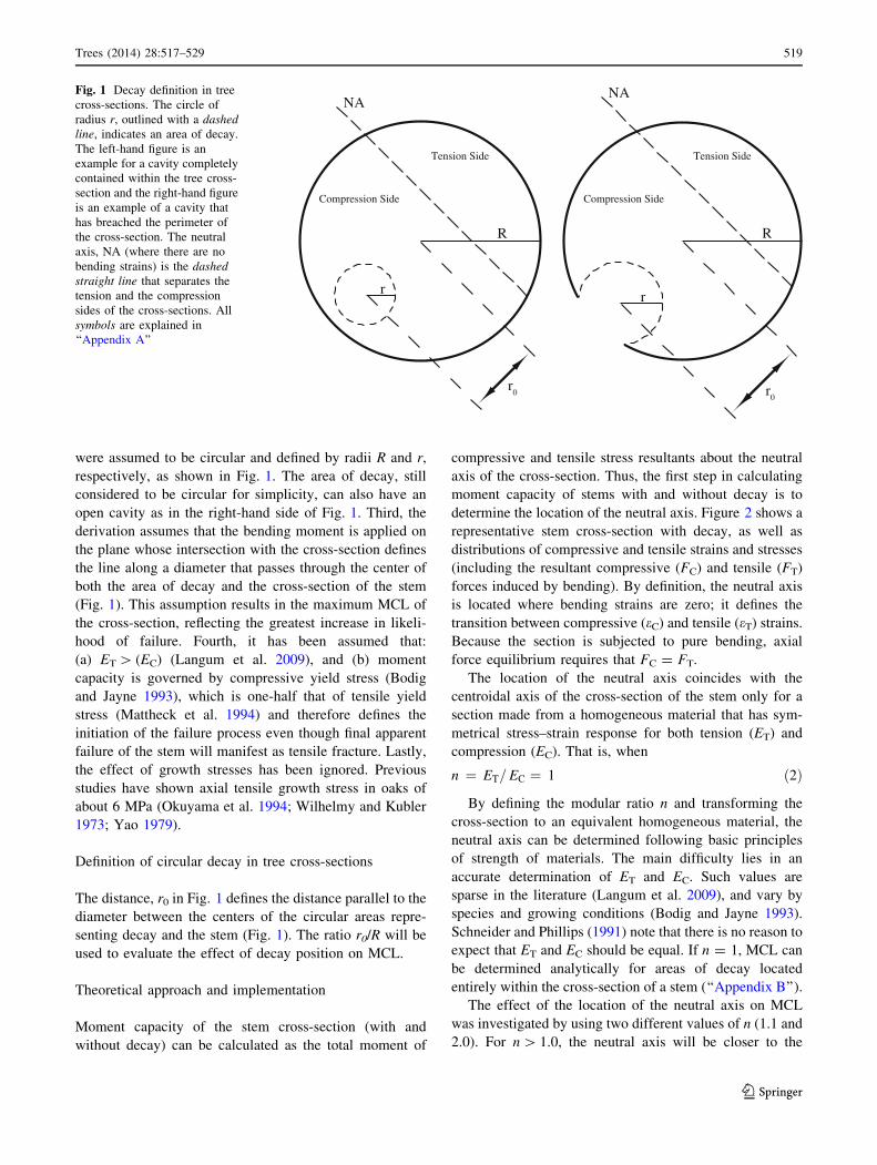
Assessment of decay shape on MCL

Although decay in trees can sometimes adopt an approxi-

mately circular or other areas with simple geometry, decay

mostly forms irregular shapes (Shigo 1984) and the extent

of decay can vary by tree species and presence of fungus

(Deflorio et al. 2008). Two methods can be used to estimate

MCL of such decayed stems using the curves developed in

this paper. The first method can be used without excessive

calculations, making it suitable for use in the field. The

second method requires a more careful accounting of the

area and location of decay.

Method I

An irregularly shaped area of decay can inscribe and be

inscribed by circles. Figure 11 shows a rectangular area of

decay, but this method can be applied to areas of any shape.

MCL can be determined from Fig. 7, assuming r and r0

from the smaller and larger circles inscribed or inscribing

the decay area. Practitioners could compare three estimates

of MCL: using the larger circle, the smaller circle, or a mean

value. Depending on the loading conditions (sheltered or

exposed trees, for example) or other factors related to risk

assessment (such as value of the target), conservative or

lenient estimates of MCL could be employed. This

approach may offer an advantage over the method described

by Mattheck et al. (1993), who suggested using the thinnest

remaining wall of sound wood when assessing off-center

areas of decay, which tended to overestimate the loss in

moment of inertia of such stems (Kane and Ryan 2004).

Method II

In this method, an irregularly shaped area of decay can be

converted into a circle of equivalent area as in Fig. 12. In

order for the method to be valid, the irregularly shaped area

of decay and its circular equivalent must share the same

centroid. After conversion to a circular area, MCL loss of

the section can be determined from Fig. 7. For simple

geometric shapes, like a rectangle, the methods will yield

very similar results because it is easy to convert the areas

into circles and determine the centroids. For irregularly

shaped areas, determining the area and centroid requires

more rigorous analysis and, likely, the use of image ana-

lysis software. For practitioners, images can be gleaned

from tomography (Gilbert and Smiley 2004; Wang and

Allison 2008), but this method requires sophisticated tools

and techniques.

r0

A

B

C

R

r

R

r

r0

Fig. 11 Description of method

I addressed in ‘‘Method I’’. As

an example, a rectangular area

of decay is shown in a circular

tree cross-section (a). Figures

b and c graphically depict how

method I can be used to

determine the upper limit and

lower limit, respectively, of

moment capacity loss of the

rectangular area of decay. All

symbols are described in

‘‘Appendix A’’

526 Trees (2014) 28:517–529

123

Conclusions

The maximum MCL of any decayed cross-section of a tree

without a noticeable lean can be approximated using

methods I or II, and Fig. 7. Similarity between (a) theo-

retically and empirically determined values of LOSSS and

(b) values of MCL calculated for a wide range of values of

n lends confidence that these methods can be reasonably

applied under a variety of field conditions. The effect of

n on estimation of MCL was negligible. Practitioners

should consider Fig. 6 to better understand the range of

variation in MCL as affected by n. Four limitations

regarding applicability of the MCL procedures described in

the paper include: (1) not accounting for axial stresses

induced by dead load and the vertical component of the

pulling tests, (2) not accounting for growth stresses and

other innate variations in wood properties (e.g., reaction

wood), (3) altered E values of wood formed after wound-

ing, and (4) presumption of the location of failure. The

ratio of axial to bending stress during the tests was minimal

(\0.1 %). The effect of growth stress may confound the

analysis of MCL in practice because of the pre-stressed

cross-section. This would especially apply to trees with

leaning stems and reaction wood since the magnitude of

growth stress would be greater (Archer 1987). Future

studies should investigate this effect, especially consider-

ing that areas of decay will alter the cross-sectional dis-

tribution of growth stress. Regarding the third limitation,

Kane and Ryan (2003) documented an increase in tough-

ness of woundwood of red maple, which may also apply to

E. Perhaps most importantly, practitioners must recognize

that MCL due to decay ignores the possibility of failure at

another location in the tree. Other defects (such as weak

branch attachments or poor root anchorage) may fail prior

to parts of the tree with decay. Thresholds for poor branch

attachments (Kane 2007, Kane et al. 2008) and root loss

(Smiley 2008) have been proposed.

The methods described in ‘‘Assessment of decay shape

on MCL’’ provide estimates of the MCL (based on

compressive yield stress) of a tree with decay. Although

some of the wood of a tree may fail in compression when

loaded, collapse and ultimate failure of the tree may not

always coincide with compressive yield (Mattheck et al.

1994; Mergen 1954). Figure 7 thus provides a more con-

servative estimate of the likelihood of tree failure, which is

preferable in the interest of avoiding injuries and property

damage. To determine whether a threshold value of MCL

existed and to further validate the predictions following the

methods presented, failed and intact branches and stems

with decay could be measured after a windstorm. Previous

attempts to find a threshold (Mattheck et al. 1993, 1994)

have been problematic (Fink 2009; Gruber 2008), so care

must be taken in sampling and analyzing such data. With a

reliable sample and normal distribution, the first and the

second moments (mean and standard deviation) of the

distribution can illustrate the MCL of different species

under wind-induced bending.

Acknowledgments This study was funded by the TREE Fund’s

Mark S. McClure Biomechanics Fellowship. Nevin Gomez, Sherry

Hu, Alex Julius, Dan Pepin, Alex Sherman, and Joseph Scharf

(University of Massachusetts-Amherst) helped collect data.

Appendix A: Acronyms and abbreviations

c Perpendicular distance from the neutral axis to a

point whose tension or compression stress will be

calculated

EC Wood compressive Young’s modulus parallel to

grain

ET Wood tensile Young’s modulus parallel to grain

FC Resultant compressive force at the compression

side in a stem cross-section

FT Resultant tensile force at the tension side in a

stem cross-section

H Height (see Fig. 4) between the puling force and

the strain meter of the experiments described in

‘‘Experiments on MCL’’

r0

R

r

R

CMCM

Circular Shaped DecayRandom Shaped Decay

Fig. 12 Description of method

II addressed in ‘‘Method II’’.

The random area of decay is

converted into a circular area.

CM refers to the geometric

center of the decay. Other

symbols are described in

‘‘Appendix A’’

Trees (2014) 28:517–529 527

123

I Moment of inertia of a cross-sectional area

computed about the neutral axis

kd The slope of the curve in Fig. 4 after notching

kud The slope of the curve in Fig. 4 before notching

M Bending moment

Md Calculated bending moment [Eq. (8)] for the

experiments (after notching) described in

‘‘Experiments on MCL’’

Mud Calculated bending moment [Eq. (8)] for the

experiments (before notching) described in

‘‘Experiments on MCL’’

n Modular ratio of ET to EC

Pd Pulling force measures from the experiments

(after notching) described in ‘‘Experiments on

MCL’’

Pud Pulling force measures from the experiments

(before notching) described in ‘‘Experiments on

MCL’’

r Radius of the circular decay defined in Fig. 1

r0 Distance between the centers of the tree section

and decayed area defined in Fig. 1

R Radius of the circular tree cross-section defined in

Fig. 1

S Section modulus of tree cross-sections

ec Strain at the outer face of the compression side in

a stem cross-section

ed Strain meter measures from the experiments (after

notching) described in ‘‘Experiments on MCL’’

et Strain at the outer face of the tension side in a

stem cross-section

eud Strain meter measures from the experiments

(before notching) described in ‘‘Experiments on

MCL’’

r Bending stress

rc-yield Yield compressive stress at the outer face of the

compression side in a stem cross-section

rt Tensile stress at the outer face of the tension side

in a stem cross-section

h Angle (see Fig. 4) between the pulling force and

the tree stem for the experiments described in

‘‘Experiments on MCL’’

Appendix B: MCL for areas of decay confined

within the cross-section

If n = 1, MCL of areas of decay confined within the cross-

section can be determined from the ratio of the section

modulus of the decay to that of the tree cross-section,

assuming each is circular. To obtain the section moduli,

first, the moments of inertia (I) for the tree cross-section

and decay area are:

I ¼ p4

R4 ð18Þ

Id ¼p4

r4 ð19Þ

in which R and r are the radii of cross-section and the

decayed area, respectively, and the subscript d indicates the

area of decay. The areas (A) of these sections are:

A ¼ pR2 ð20Þ

Ad ¼ pr2 ð21Þ

To find the location of the neutral axis (DX) of the tree

cross-section with decay:

DX ¼ Adr0

A� Ad

ð22Þ

where r0 refers to the distance between the centers of the

tree section and decayed area. The moment of inertia of the

hollow section (the tree cross-section with decay) (IH) can

be determined:

IH ¼ I � Id þ A DXð Þ2�Ad DX þ r0ð Þ2 ð23Þ

Then, the distance (c) between the circumference of tree

cross-section and the neutral axis is:

c ¼ Rþ DX ð24Þ

Finally, loss of section modulus can be calculated as:

sloss ¼I=R� IH=c

I=Rð25Þ

References

Archer RR (1987) Growth stresses and strains in trees. Springer in

wood science. Springer-Verlag, Berlin

Bodig J, Jayne BA (1993) Mechanics of wood and wood composites.

Krieger Publishing Company, Malabar

Butnor JR, Pruyn ML, Shaw DC, Harmon ME, Mucciardi AN, Ryan

MG (2009) Detecting defects in conifers with ground penetrating

radar: applications and challenges. For Pathol 39:309–322

Coder KD (1989) Should you or shouldn’t you fill tree hollows?

Grounds Maint 24(9):68–70

Deflorio G, Johnson C, Fink S, Schwarze FWMR (2008) Decay

development in living sapwood of coniferous and deciduous

trees inoculated with six wood decay fungi. For Ecol Manage

255(7):2373–2383. doi:10.1016/j.foreco.2007.12.040

Fink S (2009) Hazard tree identification by visual tree assessment

(Vta): scientifically solid and practically approved. Arboric J

32(3):139–155. doi:10.1080/03071375.2009.9747570

Gilbert EA, Smiley ET (2004) Picus sonic tomography for the

quantification of decay in white oak (Quercus alba) and hickory

(Carya spp.). J Arboric 30:277–281

Glaberson W, Foderado LW (2012) Neglected, rotting trees turn

deadly. The New York Times, New York

Gruber F (2008) Reply to the response of Claus Mattheck and Klaus

Bethge to my criticisms on untenable vta-failure criteria, who is

right and who is wrong? Arboric J 31(4):277–296

528 Trees (2014) 28:517–529

123

James K (2003) Dynamic loadig of trees. J Arboric 29(3):165–171

James KR, Kane B (2008) Precision digital instruments to measure

dynamic wind loads on trees during storms. J Arboric

148(6–7):1055–1061. doi:10.1016/j.agrformet.2008.02.003

Johnstone D, Tausz M, Moore G, Nicolas M (2010) Quantifying

wood decay in Sydney Bluegum (Eucalyptus saligna) trees.

Arvoric Urban For 36(6):243–252

Jullien D, Widmann R, Loup C, Thibaut B (2013) Relationship

between tree morphology and growth stress in mature European

beech stands. Ann For Sci 70(2):133–142. doi:10.1007/s13595-

012-0247-7

Kane B (2007) Branch strength of Bradford pear (Pyrus calleryana

var. ‘Bradford’). Arboric Urban For 33(4):283–291

Kane B, Ryan D (2003) Examining formulas that assess strength loss

due to decay in trees: woundwood toughness improvement in red

maple (Acer rubrum). J Arboric 29(4):207–217

Kane B, Ryan D (2004) The accuracy of formulas used to assess

strength loss due to decay in trees. J Arboric 30(6):347–356

Kane B, Ryan D, Bloniarz DV (2001) Comparing formulae that assess

strength loss due to decay in trees. J Arboric 27(2):78–87

Kane B, Farrell R, Zedaker SM, Loferski JR, Smith DW (2008)

Failure mode and prediction of the strength of branch attach-

ments. Arboric Urban For 34(5):308–316

Kretschmann DE (2010) Mechanical properties of wood. In: Wood

handbook, wood as an engineering material, vol 5. Department

of Agriculture, Forest Service, Forest Products Laboratory,

Madison, pp 1–46

Langum CE, Yadama V, Lowell EC (2009) Physical and mechanical

properties of young-growth Douglas-fir and western hemlock

from western Washington. For Prod J 59(11/12):37–47

Langwig JE, Meyer JA, Davidson RW (1968) Influence of polymer

impregnation on mechanical properties of basswood. For Prod J

18(7):31–36

Mattheck C, Bethge K, Erb D (1993) Failure criteria for trees. Arboric

J 17:201–209

Mattheck C, Lonsdale D, Breloer H (1994) The body language of

trees: a handbook for failure analysis. HMSO, London

Mergen F (1954) Mechanical aspects of wind-breakage and wind-

firmness. J For 52(2):119–125

Mortimer MJ, Kane B (2004) Hazard tree liability in the United

States: uncertain risks for owners and professionals. Urban For

Urban Green 2(3):159–165. doi:10.1078/1618-8667-00032

Nicolotti G, Socco LV, Martinis R, Godio A, Sambuelli L (2003)

Application and comparison of three tomographic techniques for

detection of decay in trees. J Arboric 29(2):66–78

Okuyama T, Yamamoto H, Yoshida M, Hattori Y, Archer R (1994)

Growth stresses in tension wood: role of microfibrils and

lignification. Ann For Sci 51(3):291–300

Ozyhar T, Hering S, Niemz P (2013) Moisture-dependent orthotropic

tension-compression asymmetry of wood. Holzforschung, vol

67. doi:10.1515/hf-2012-0089

Peltola HM (2006) Mechanical stability of trees under static loads.

Am J Bot 93(10):1501–1511. doi:10.3732/ajb.93.10.1501

Ruel J-C, Achim A, Herrera R, Cloutier A (2010) Relating

mechanical strength at the stem level to values obtained from

defect-free wood samples. Trees 24(6):1127–1135. doi:10.1007/

s00468-010-0485-y

Schmidlin T (2009) Human fatalities from wind-related tree failures

in the United States, 1995–2007. Nat Hazards 50(1):13–25.

doi:10.1007/s11069-008-9314-7

Schneider MH, Phillips JG (1991) Elasticity of wood and wood

polymer composites in tension compression and bending. Wood

Sci Technol 25(5):361–364. doi:10.1007/BF00226175

Schneider MH, Phillips JG, Tingley DA, Brebner KI (1990)

Mechanical properties of polymer-impregnated sugar maple.

For Prod J 40(1):37–41

Shigo AL (1984) How to assess the defect status of a stand. North J

Appl For 1(3):41–49

Sinn G, Wessolly L (1989) A contribution to the proper assessment of

the strength and stability of trees. Arboric J 13:45–65

Smiley ET (2008) Root pruning and stability of young willow oak.

Arboric Urban For 34(2):123–128

Smiley ET, Fraedrich BR (1992) Determining strength loss from

decay. J Arboric 18(4):201–204

Wagener WW (1963) Judging hazard from native trees in California

recreational areas: a guide for professional foresters. US Forest

Service Research Paper, PSW-P1, p 29

Wang X, Allison RB (2008) Decay detection in red oak trees using a

combination of visual inspection, acoustic testing, and resistance

microdrilling. Arboric Urban For 34(1):1–4

Wilhelmy V, Kubler H (1973) Stresses and checks in log ends from

relieved growth stresses. Wood Sci 6:136–142

Wilson BF, Gartner BL (1996) Lean in red alder (Alnus rubra):

growth stress, tension wood, and righting response. Can J For

Res 26(11):1951–1956

Yao J (1979) Relationships between height and growth stresses within

and among white ash, water oak, and shagbark hickory. Wood

Sci 11(4):246–251

Yoshida M, Ohta H, Okuyama T (2002) Tensile growth stress and

lignin distribution in the cell walls of black locust (Robinia

pseudoacacia). J Wood Sci 48(2):99–105. doi:10.1007/

BF00767285

Trees (2014) 28:517–529 529

123