lorenzo magnea
TRANSCRIPT
PROGRESS ON THE FIELD THEORY LIMIT OF PERTURBATIVE MULTI-LOOP STRING AMPLITUDES
Lorenzo Magnea
University of Torino - INFN Torino
Scattering Amplitudes, ECT* Trento, 16/07/12
Outline
• On string amplitudes
• One- and two-loop examples
• Effective actions in background fields
• Picking diagrams from strings
• Results and outlook
Work in collaboration with R. Russo (QMUL) and S. Sciuto (Torino)
ON STRING AMPLITUDES
ON STRING AMPLITUDES
``Strings is a mythological story about the son of a king ... ‘’
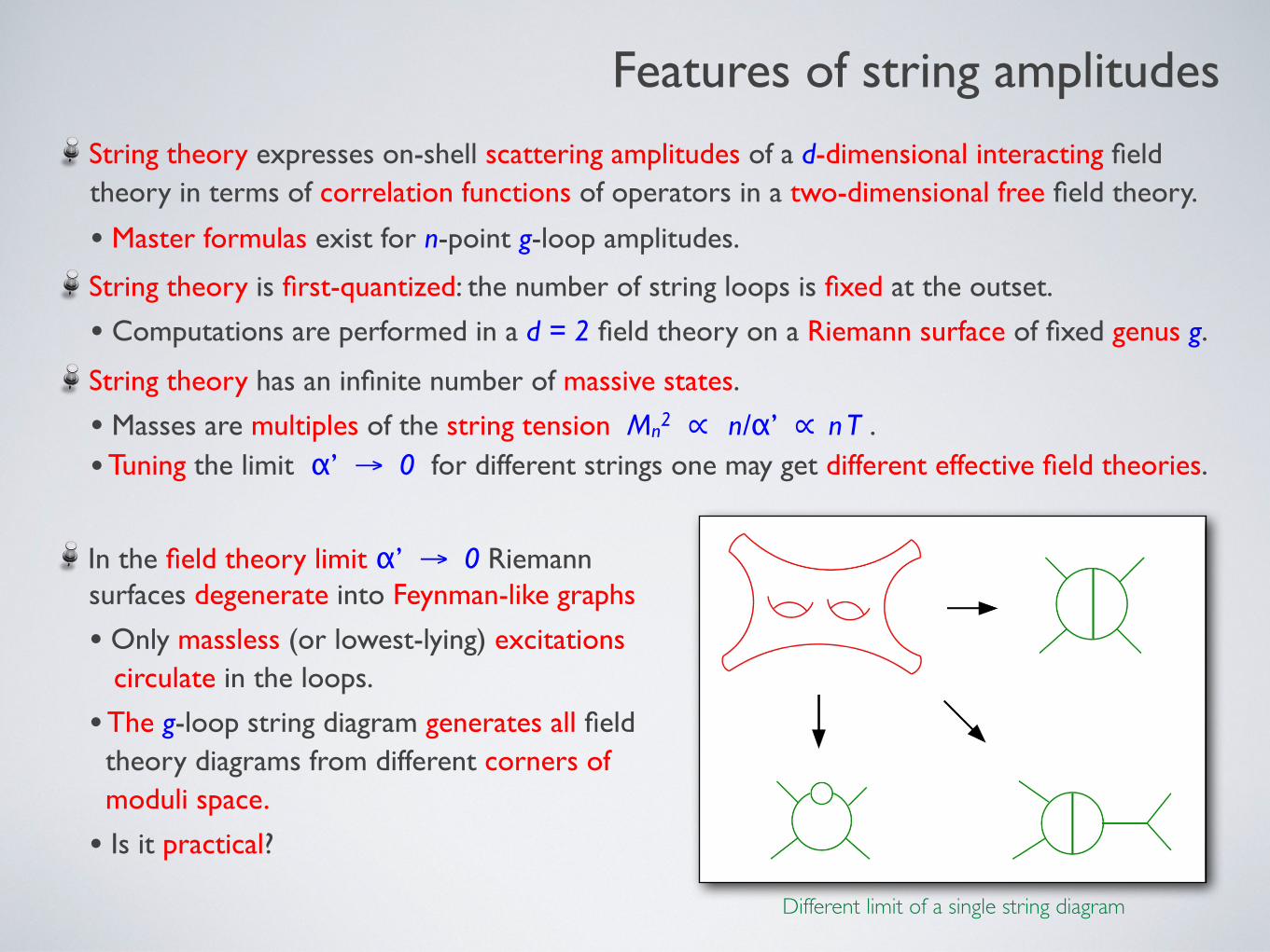
String theory expresses on-shell scattering amplitudes of a d-dimensional interacting field theory in terms of correlation functions of operators in a two-dimensional free field theory.
• Master formulas exist for n-point g-loop amplitudes.
String theory is first-quantized: the number of string loops is fixed at the outset.
• Computations are performed in a d = 2 field theory on a Riemann surface of fixed genus g.
String theory has an infinite number of massive states.
• Masses are multiples of the string tension Mn2 ∝ n/α’ ∝ n T .
• Tuning the limit α’ → 0 for different strings one may get different effective field theories.
Features of string amplitudes
In the field theory limit α’ → 0 Riemann surfaces degenerate into Feynman-like graphs
• Only massless (or lowest-lying) excitations circulate in the loops.
• The g-loop string diagram generates all field theory diagrams from different corners of moduli space.
• Is it practical?
Different limit of a single string diagram
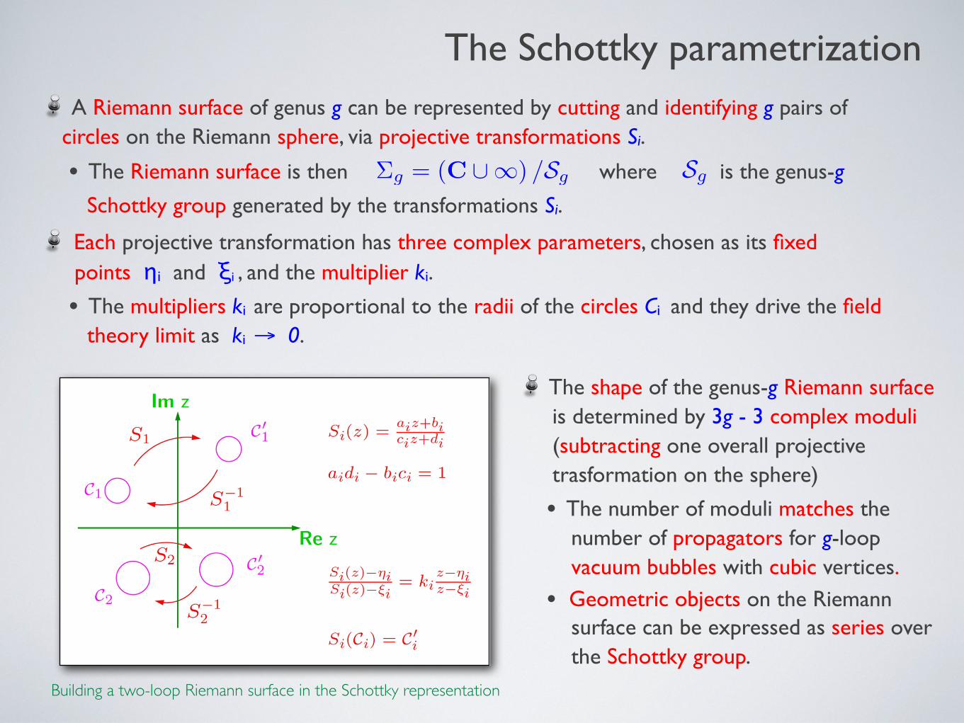
The Schottky parametrization A Riemann surface of genus g can be represented by cutting and identifying g pairs of
circles on the Riemann sphere, via projective transformations Si.
• The Riemann surface is then where is the genus-g
Schottky group generated by the transformations Si.
Each projective transformation has three complex parameters, chosen as its fixed points ηi and ξi , and the multiplier ki.
• The multipliers ki are proportional to the radii of the circles Ci and they drive the field theory limit as ki → 0.
⌃g = (C [1) /Sg Sg
Building a two-loop Riemann surface in the Schottky representation
The shape of the genus-g Riemann surface is determined by 3g - 3 complex moduli (subtracting one overall projective trasformation on the sphere)
• The number of moduli matches the number of propagators for g-loop vacuum bubbles with cubic vertices.
• Geometric objects on the Riemann surface can be expressed as series over the Schottky group.

Geometric objects
The string operator formalism provides explicit constructions for geometric objects defined on Riemann surfaces, in terms of series on the Schottky group.
Let be an element of the Schottky group. Then one defines
Abelian Differentials:
Period Matrix:
Prime Form:
Scalar Propagator:
• In the field theory limit only a handful of Schottky group elements contribute.
• Relevant terms are easily generated with available software for symbolic manipulations.
!µ =
(µ)X
↵
✓1
z � T↵(⌘µ)� 1
z � T↵(⇠µ)
◆dz
⌧µ⌫ =1
2⇡i
Z
b⌫
!µ(z)
Eg(z, w)pdzdw = (z � w)
Y↵
z � T↵(w)
z � T↵(z)
w � T↵(z)
w � T↵(w)
Gg(z, w) = log [Eg(z, w)]�1
2
Z w
z!µ
h(2⇡ Im⌧)�1
iµ⌫ Z w
z!⌫
T↵ = Sai · Sb
j · . . .
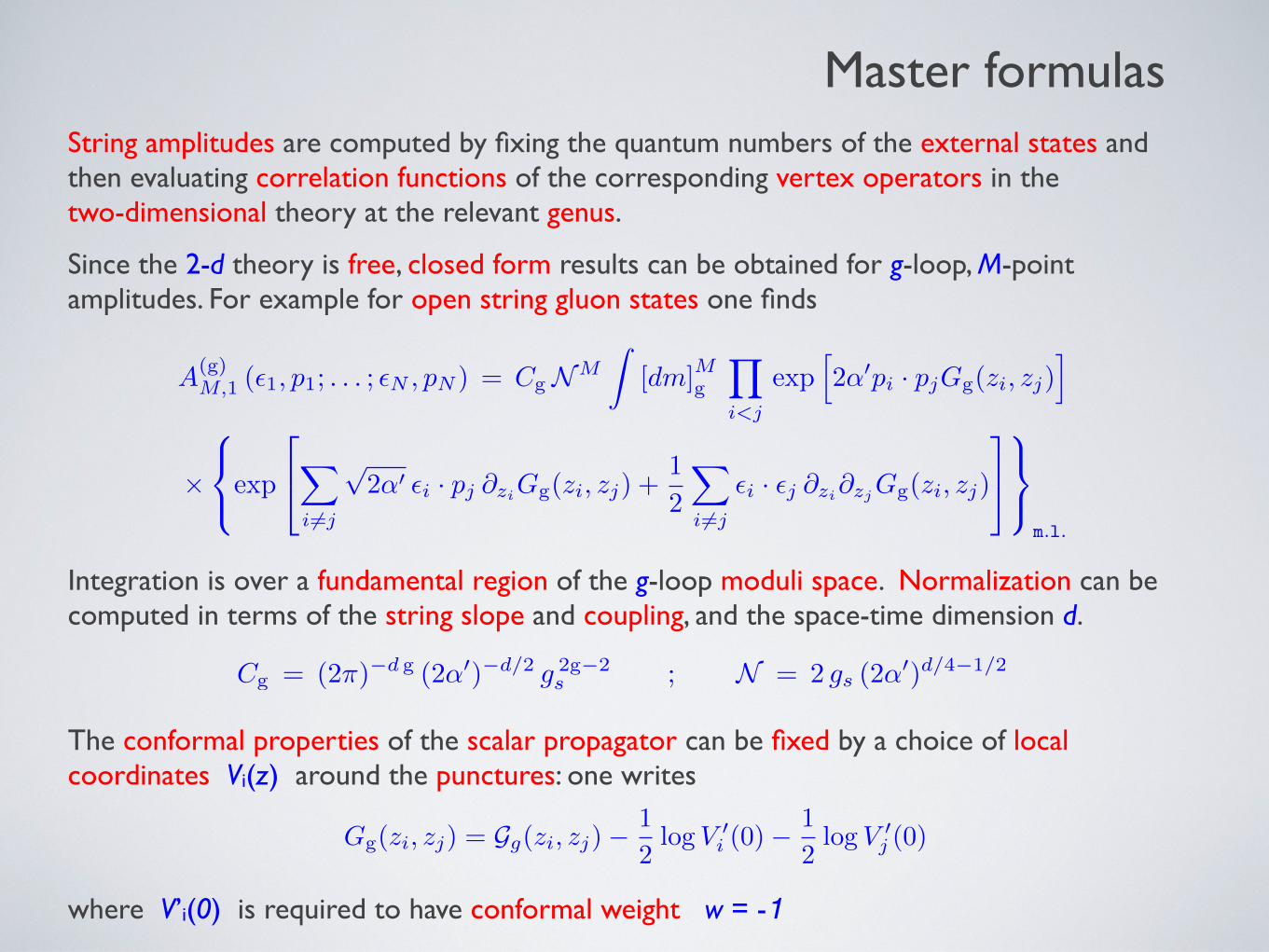
Master formulasString amplitudes are computed by fixing the quantum numbers of the external states and then evaluating correlation functions of the corresponding vertex operators in the two-dimensional theory at the relevant genus.
Since the 2-d theory is free, closed form results can be obtained for g-loop, M-point amplitudes. For example for open string gluon states one finds
Integration is over a fundamental region of the g-loop moduli space. Normalization can becomputed in terms of the string slope and coupling, and the space-time dimension d.
The conformal properties of the scalar propagator can be fixed by a choice of localcoordinates Vi(z) around the punctures: one writes
where V’i(0) is required to have conformal weight w = -1
A(g)M,1 (✏1, p1; . . . ; ✏N , pN ) = Cg NM
Z[dm]
Mg
Y
i<j
exp
h2↵0pi · pjGg(zi, zj)
i
⇥
8<
:exp
2
4X
i 6=j
p2↵0 ✏i · pj @ziGg(zi, zj) +
1
2
X
i 6=j
✏i · ✏j @zi@zjGg(zi, zj)
3
5
9=
;m.l.
Cg = (2⇡)�d g (2↵0)�d/2 g 2g�2s ; N = 2 gs (2↵
0)d/4�1/2
Gg(zi, zj) = Gg(zi, zj)�1
2
log V 0i (0)�
1
2
log V 0j (0)
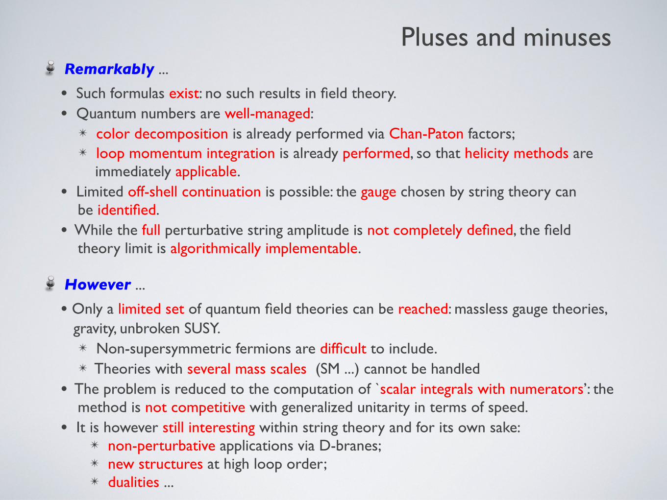
Pluses and minuses Remarkably ...
• Such formulas exist: no such results in field theory.• Quantum numbers are well-managed:
✴ color decomposition is already performed via Chan-Paton factors;✴ loop momentum integration is already performed, so that helicity methods are
immediately applicable.• Limited off-shell continuation is possible: the gauge chosen by string theory can
be identified.• While the full perturbative string amplitude is not completely defined, the field
theory limit is algorithmically implementable.
However ...
• Only a limited set of quantum field theories can be reached: massless gauge theories, gravity, unbroken SUSY.
✴ Non-supersymmetric fermions are difficult to include.✴ Theories with several mass scales (SM ...) cannot be handled• The problem is reduced to the computation of `scalar integrals with numerators’: the
method is not competitive with generalized unitarity in terms of speed.• It is however still interesting within string theory and for its own sake:
✴ non-perturbative applications via D-branes;✴ new structures at high loop order;✴ dualities ...

ONE-LOOP GLUON AMPLITUDES
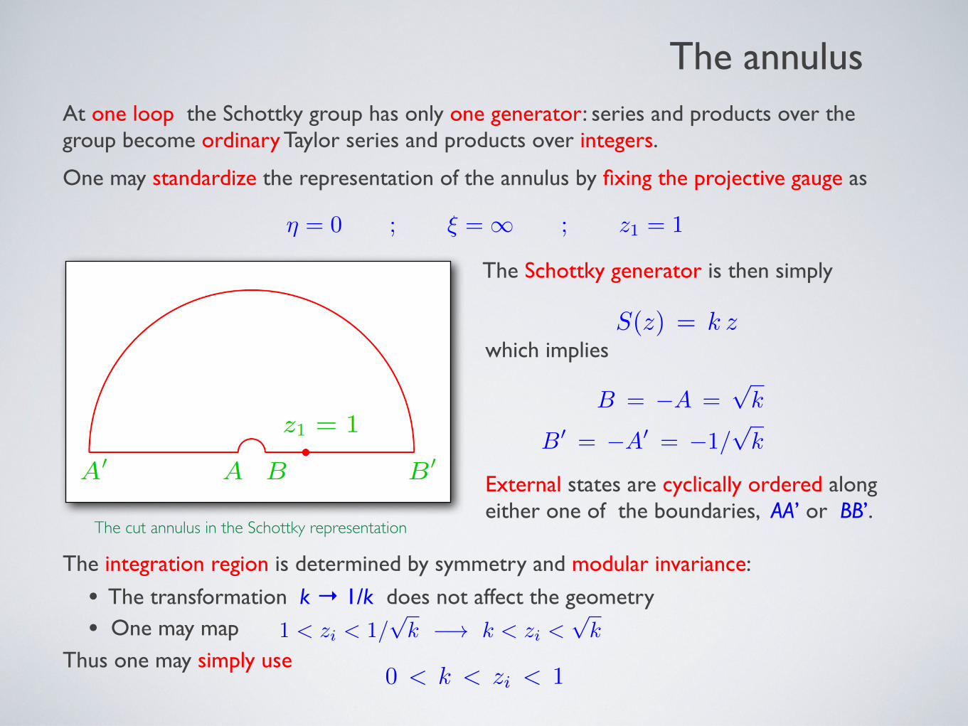
The annulusAt one loop the Schottky group has only one generator: series and products over the group become ordinary Taylor series and products over integers.
One may standardize the representation of the annulus by fixing the projective gauge as
The Schottky generator is then simply which implies
External states are cyclically ordered along either one of the boundaries, AA’ or BB’.
The integration region is determined by symmetry and modular invariance:
• The transformation k → 1/k does not affect the geometry
• One may map Thus one may simply use
⌘ = 0 ; ⇠ = 1 ; z1 = 1
The cut annulus in the Schottky representation
S(z) = k z
B = �A =pk
B0 = �A0 = �1/pk
1 < zi < 1/pk �! k < zi <
pk
0 < k < zi < 1

One-loop master formula
The ingredients of the one-loop master formula for gluons are easily determined
Measure of integration
Matching the string and the strong coupling, from tree level
The scalar propagator
where the choice
insures modular invariance
[dm]
M1 =
1
k2
1Y
n=1
(1� kn)2�d
✓� log k
2
◆� d2
MY
i=2
dzi ⇥ (zi � zi+1)
gs =1
2gd (2↵
0)1�d/4
G(zi, zj) = log
✓����r
zizj
�r
zjzi
����
◆+
1
2 log k
✓log
zizj
◆2
+ log
2
41Y
n=1
⇣1� kn zj
zi
⌘⇣1� kn zi
zj
⌘
(1� kn)2
3
5
V 0i (0) = (!(zi))
�1 = zi
G(zi/zj ; k) = G(zj/zi; k) = G(kzi/zj ; k)

The field theory limit From the string operator formalism we know that Laurent expansion of the integrand in
powers of k counts the mass level of the state propagating in the loop.
The master formula has an overall power of α’. String moduli defining the shape of the surface must be expressed in units of α’ , in order to take the limit α’ → 0
• Hint: measure of integration is d log k ...
Pedestrian field theory limit (exact for scalars):
• Note: t and ti will be identified with with sums of Schwinger parameters associated with propagators around the loop.
For gluons, the overall power p of α’ after the change of variables is not uniform: instead, - M/2 < p < 0 . One must locate all further sources of positive powers of α’ .
• Four-point vertices
• Expansion of the exponential
log k = � t
↵0 ; log zi = � ti↵0
exp
h2↵0 pi · pj Gij
i�! exp
hc0(ti) + ↵0c1(ti)
i
k�2 �! tachyon ; k�1 �! gluon ; . . .
(ti � ti�1)/↵0 = O(1)
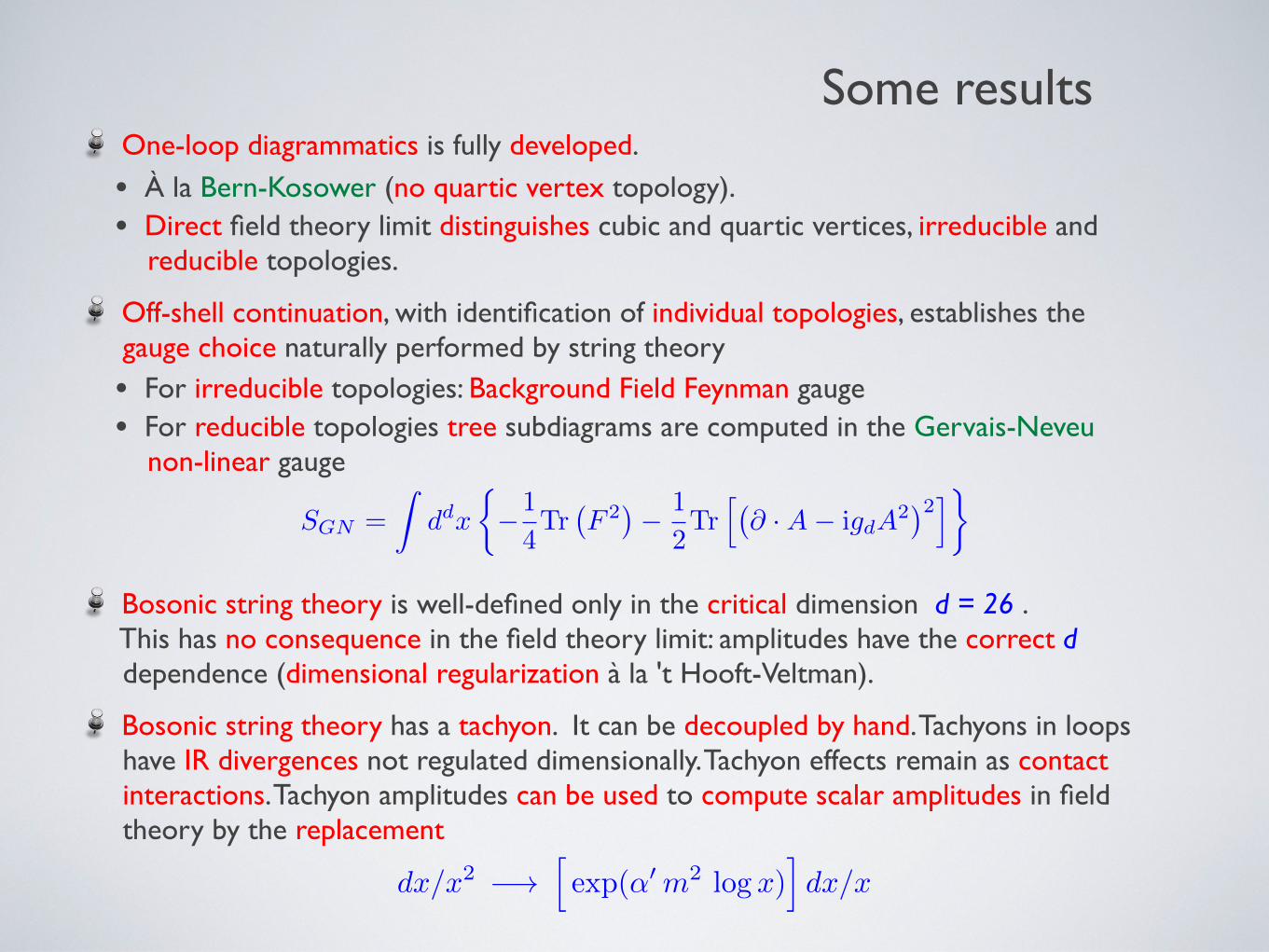
Some results One-loop diagrammatics is fully developed.
• À la Bern-Kosower (no quartic vertex topology).• Direct field theory limit distinguishes cubic and quartic vertices, irreducible and
reducible topologies.
Off-shell continuation, with identification of individual topologies, establishes the gauge choice naturally performed by string theory
• For irreducible topologies: Background Field Feynman gauge• For reducible topologies tree subdiagrams are computed in the Gervais-Neveu
non-linear gauge
Bosonic string theory is well-defined only in the critical dimension d = 26 . This has no consequence in the field theory limit: amplitudes have the correct d dependence (dimensional regularization à la 't Hooft-Veltman).
Bosonic string theory has a tachyon. It can be decoupled by hand. Tachyons in loops have IR divergences not regulated dimensionally. Tachyon effects remain as contact interactions. Tachyon amplitudes can be used to compute scalar amplitudes in field theory by the replacement
SGN =
Zd
dx
⇢�1
4Tr
�F
2�� 1
2Tr
h�@ ·A� igdA
2�2i
�
dx/x
2 �!hexp(↵
0m
2log x)
idx/x

TWO-LOOP AMPLITUDES

The double annulusAt two loops the Schottky group has two generators: however expanding in powers of the multipliers remains simple since Si ( Si (z) ) contributes to order ki
2.
One may standardize the representation of the double annulus by choosing the gauge as
The Schottky generators are then and
It is possible to identify precisely on which propagator and on which boundary the punctures are inserted
Insertion on different boundaries yields different expressions for the integrand of the amplitude, but the results are related by modular transformations, providing highly nontrivial checks on the field theory limit.
⌘1 = 0 ; ⇠1 = 1 ; ⇠2 = 1
The cut double annulus in the Schottky representation
S2(z) =⌘(1� z) + k2(z � ⌘)
(1� z) + k2(z � ⌘)
S1(z) = k1 z
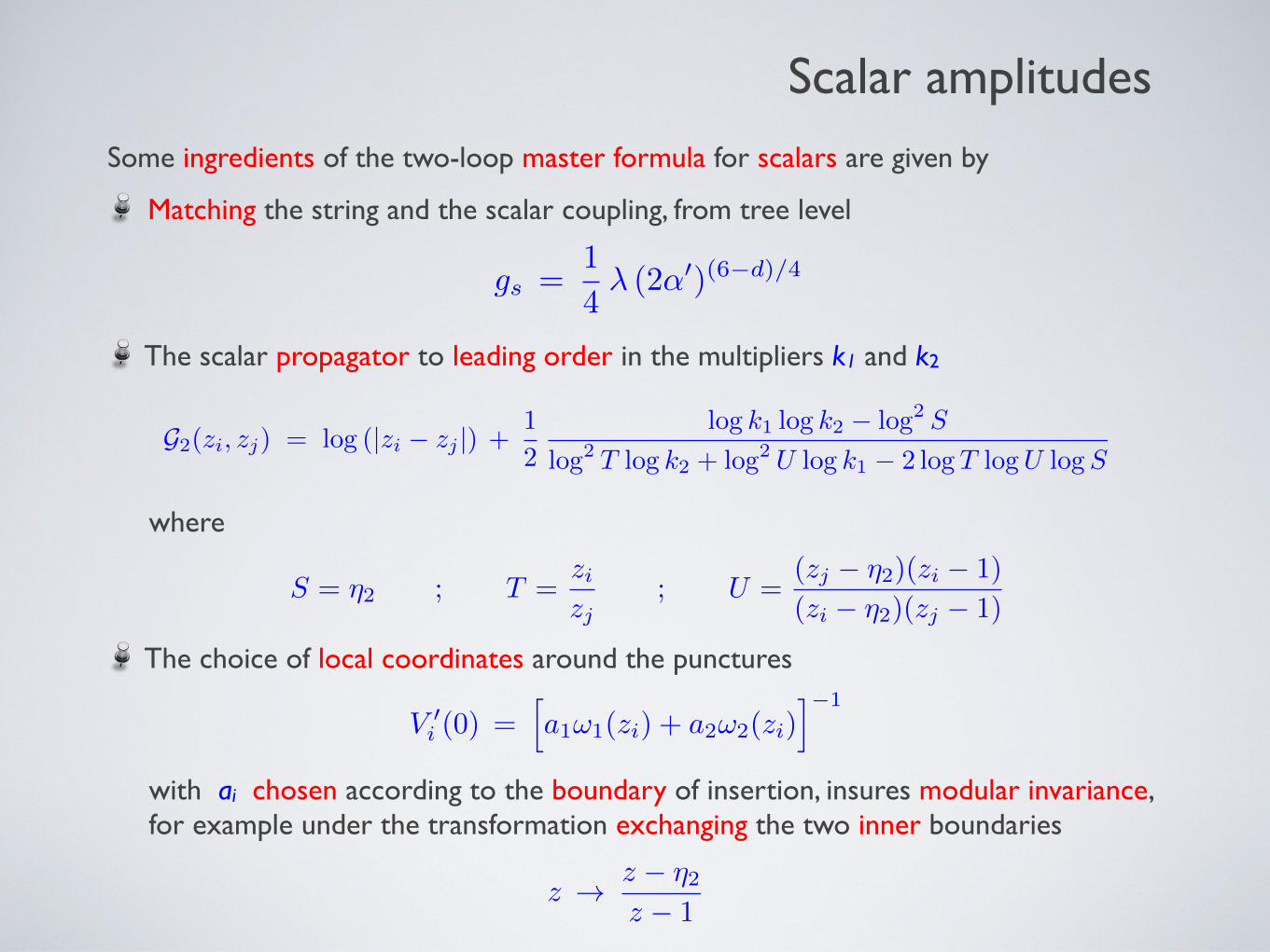
Scalar amplitudesSome ingredients of the two-loop master formula for scalars are given by
Matching the string and the scalar coupling, from tree level
The scalar propagator to leading order in the multipliers k1 and k2
where
The choice of local coordinates around the punctures
with ai chosen according to the boundary of insertion, insures modular invariance, for example under the transformation exchanging the two inner boundaries
gs =1
4� (2↵0)(6�d)/4
G2(zi, zj) = log (|zi � zj |) +
1
2
log k1 log k2 � log
2 S
log
2 T log k2 + log
2 U log k1 � 2 log T logU logS
S = ⌘2 ; T =zizj
; U =(zj � ⌘2)(zi � 1)
(zi � ⌘2)(zj � 1)
V 0i (0) =
ha1!1(zi) + a2!2(zi)
i�1
z ! z � ⌘2z � 1

In the two relevant regions dimensionful proper-time variables are defined as
The integration region is found requiring that Schottky circles do not overlap, and simplifiesin the field theory limit. Regulating tachyon double poles by treating m2 as generic one finds
which as expected agrees with field theory, including color and symmetry factors.
Vacuum bubbles
⌘1 ! 1 : ki = e�ti/↵0
; 1� ⌘1 = e�t3/↵0
⌘1 ! 0 : qi ⌘ ki/⌘1 = e�ti/↵0
; q3 ⌘ ⌘1 = e�t3/↵0
D1 =N3
(4⇡)dg2
32
Z 1
0dt3
Z 1
0dt2
Z t2
0dt1 e
�m2(t1+t2+t3) (t1t2)�d/2
D2 =N3
(4⇡)dg2
32
Z 1
0dt3
Z t3
0dt2
Z t2
0dt1 e
�m2(t1+t2+t3) (t1t2 + t1t3 + t2t3)�d/2
Topologies for scalar two-loop vacuum bubbles
Leading regions in the field theory limitarise as ki → 0 , and
The fixed point η1 plays the role of `distance between the loops’.
⌘1 ! 0 or ⌘1 ! 1

EFFECTIVE ACTIONS
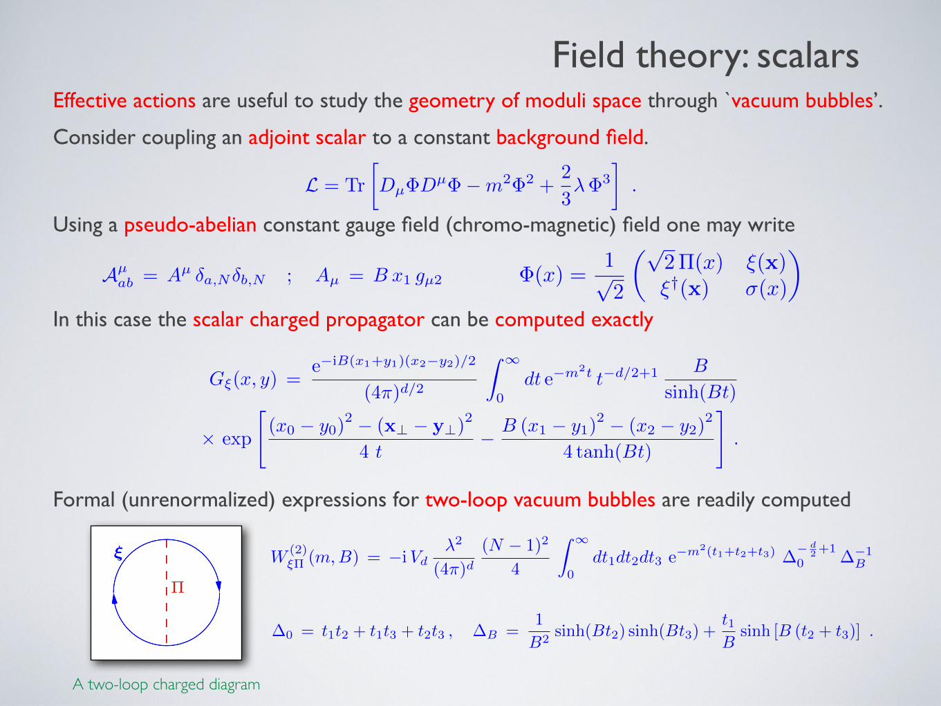
Effective actions are useful to study the geometry of moduli space through `vacuum bubbles’.
Consider coupling an adjoint scalar to a constant background field.
Using a pseudo-abelian constant gauge field (chromo-magnetic) field one may write
In this case the scalar charged propagator can be computed exactly
Formal (unrenormalized) expressions for two-loop vacuum bubbles are readily computed
Field theory: scalars
L = Tr
Dµ�D
µ��m2�2 +2
3��3
�.
Aµab = A
µ�a,N�b,N ; Aµ = B x1 gµ2 �(x) =
1p2
✓p2⇧(x) ⇠(x)⇠
†(x) �(x)
◆
G
⇠
(x, y) =
e
�iB(x1+y1)(x2�y2)/2
(4⇡)
d/2
Z 1
0dt e
�m
2t
t
�d/2+1 B
sinh(Bt)
⇥ exp
"(x0 � y0)
2 � (x? � y?)2
4 t
� B (x1 � y1)2 � (x2 � y2)
2
4 tanh(Bt)
#.
W (2)⇠⇧ (m,B) = �iVd
�2
(4⇡)d(N � 1)2
4
Z 1
0dt1dt2dt3 e�m2(t1+t2+t3) �
� d2+1
0 ��1B
�0 = t1t2 + t1t3 + t2t3 , �B =1
B2sinh(Bt2) sinh(Bt3) +
t1B
sinh [B (t2 + t3)] .
A two-loop charged diagram

A more challenging and interesting calculation is pure Yang-Mills theory,
With string theory in mind, we pick an intricate gauge (Bern, Dunbar), the background field version of the Gervais-Neveu gauge
In this form, it is (almost) the most general gauge choice compatible with the BF method.
As before, we take a block-diagonal gauge field, non-trivial in a fixed plane.
The gluon propagator has charged polarizations, which can be diagonalized
Not withstanding a (well-known) instability, computations can be formally carried out:
Field theory: gauge bosons
L = � 1
2Tr
hF 2
(A+Q)
i� 1
⇠Tr
hG2(A,Q)
i+ L
ghost
G(A,Q) = D(A)µ Qµ +
i
2↵ g {Qµ, Q
µ}
A
(i)µ = �aibi B
(i)x1 gµ2 �! F
(A)12 = diag
n
B
(i)o
G
+ij(x, y) = �g
+�G⇠(x, y) , with B ! Bi �Bj , e�m2t ! e�2(Bi�Bj)t
=
g2
(4⇡)dN1N2N3 Vd
1 + ↵2
2
(d� 2)
Z 1
0dt1dt2dt3
t1 + t2 + t3
�
d/20 �B
Q3i=1 cosh
�Biti
�
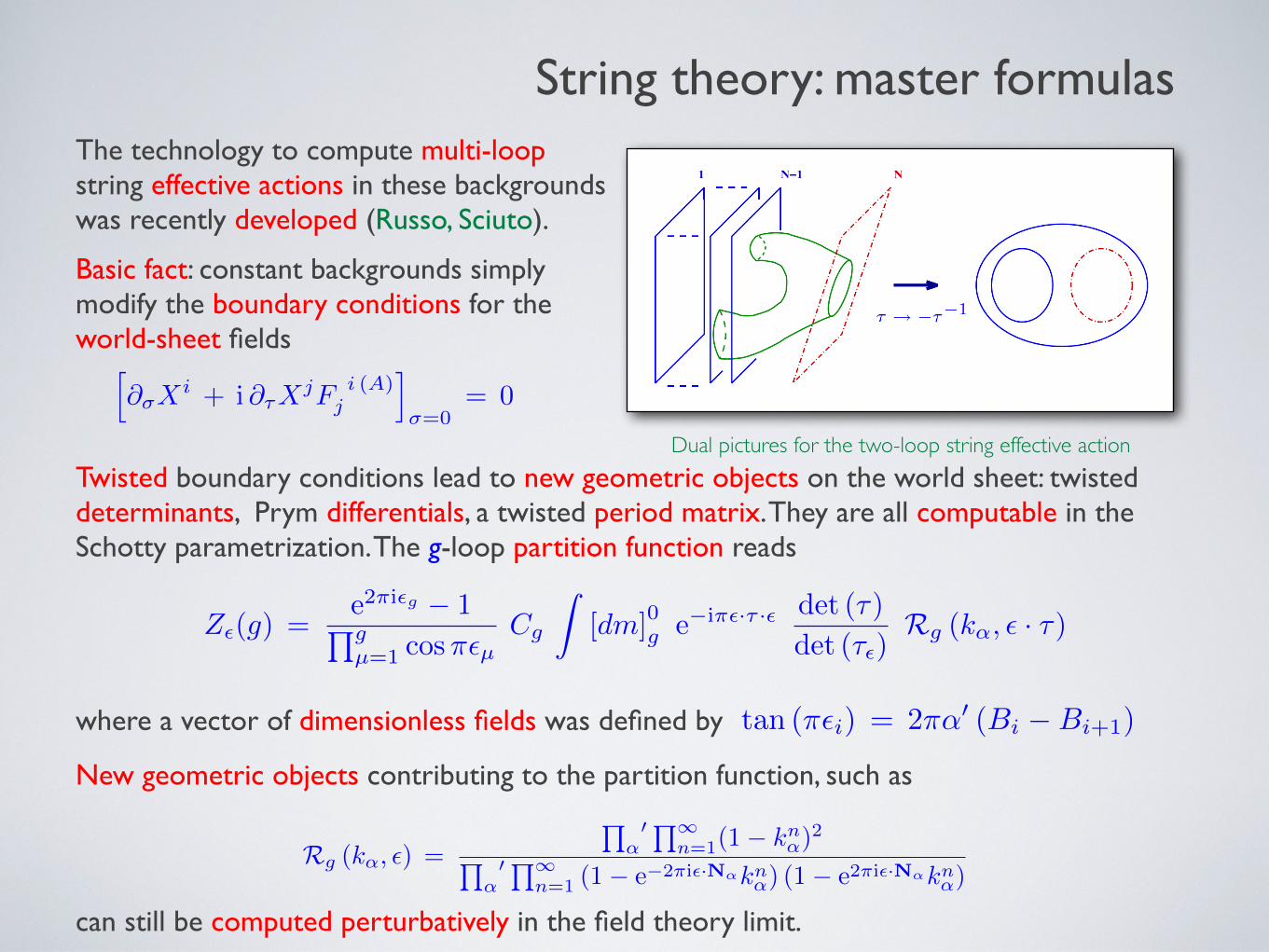
The technology to compute multi-loopstring effective actions in these backgroundswas recently developed (Russo, Sciuto).
Basic fact: constant backgrounds simply modify the boundary conditions for theworld-sheet fields
Twisted boundary conditions lead to new geometric objects on the world sheet: twisted determinants, Prym differentials, a twisted period matrix. They are all computable in the Schotty parametrization. The g-loop partition function reads
where a vector of dimensionless fields was defined by
New geometric objects contributing to the partition function, such as
can still be computed perturbatively in the field theory limit.
String theory: master formulas
h@�X
i + i @⌧XjF i (A)
j
i
�=0= 0
Z✏(g) =
e
2⇡i✏g � 1Qgµ=1 cos⇡✏µ
Cg
Z[dm]
0g e
�i⇡✏·⌧ ·✏ det (⌧)
det (⌧✏)Rg (k↵, ✏ · ⌧)
Rg (k↵, ✏) =
Q↵0 Q1
n=1(1� kn↵)2
Q↵0 Q1
n=1 (1� e�2⇡i✏·N↵kn↵) (1� e2⇡i✏·N↵kn↵)
Dual pictures for the two-loop string effective action
tan (⇡✏i) = 2⇡↵0 (Bi �Bi+1)

The difficulty in extending two-loop calculationsbeyond the string ground state can be traced toa failure of the pedestrian choice of variables forthe field theory limit
A better choice is dictated by geometry, and modular invariance: each boundary must bedecomposed as the product of two propagatorsin a modularly covariant way
One can postulate an exact factorization of themultipliers associated with each boundary as
The third definition appears to lead to complicated square-root singularities. Remarkably,it can be simply inverted as
The field theory limit for this topology is then driven by expanding in pi , using
Picking the right variables
k (S1) ⌘ p1 p3 , k (S2) ⌘ p2 p3 , k�S1 · S�1
2
�⌘ p1 p2 ,
k1 = p1 p3 , k2 = p2 p3 , ⌘ =(1 + p1) (1 + p2) p3(1 + p3) (1 + p1p2p3)
Schottky actions on the two-loop annulus
log pi ⌘ �ti/↵0
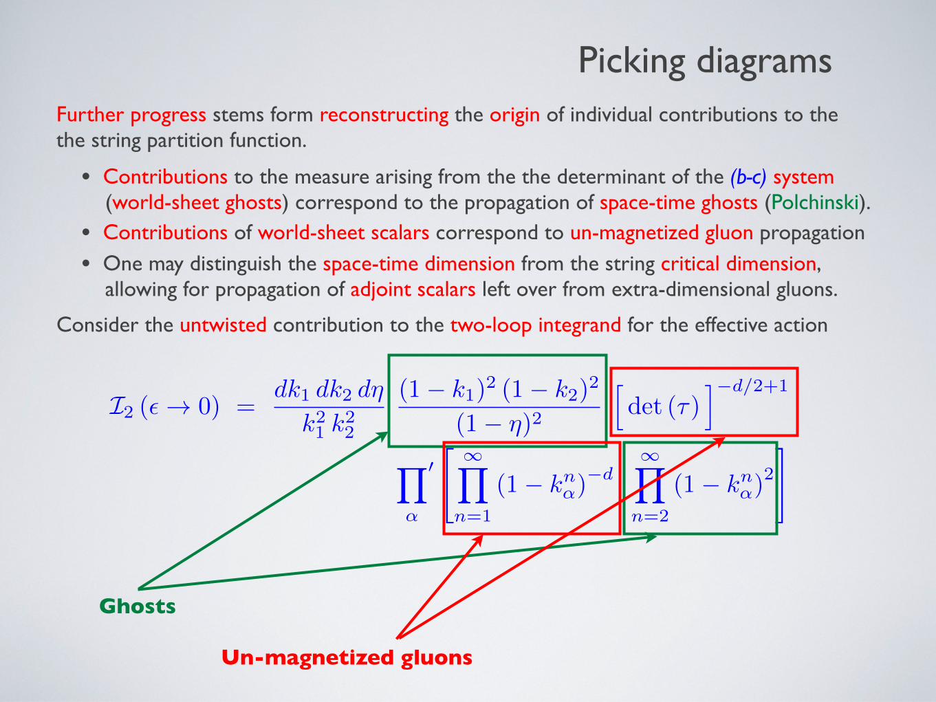
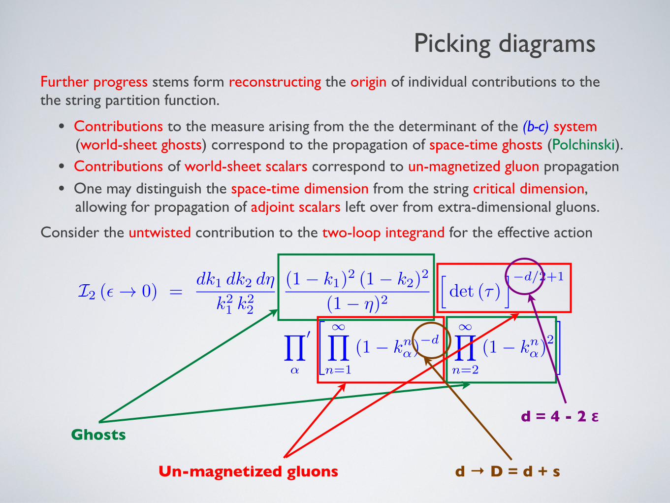
Further progress stems form reconstructing the origin of individual contributions to thethe string partition function.
• Contributions to the measure arising from the the determinant of the (b-c) system (world-sheet ghosts) correspond to the propagation of space-time ghosts (Polchinski).
• Contributions of world-sheet scalars correspond to un-magnetized gluon propagation
• One may distinguish the space-time dimension from the string critical dimension, allowing for propagation of adjoint scalars left over from extra-dimensional gluons.
Picking diagrams
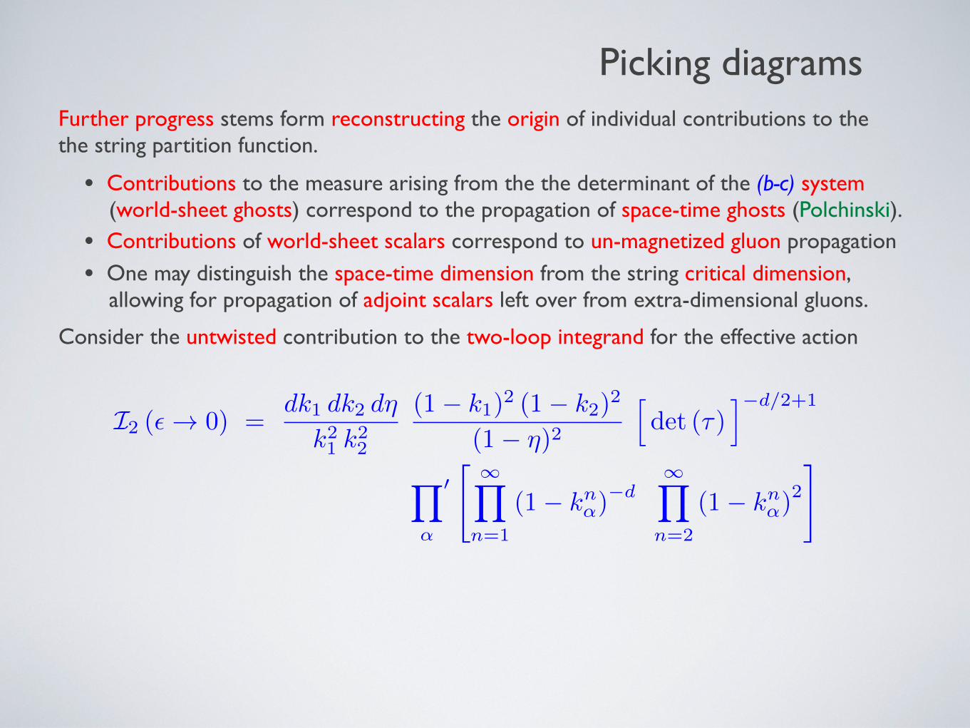
Further progress stems form reconstructing the origin of individual contributions to thethe string partition function.
• Contributions to the measure arising from the the determinant of the (b-c) system (world-sheet ghosts) correspond to the propagation of space-time ghosts (Polchinski).
• Contributions of world-sheet scalars correspond to un-magnetized gluon propagation
• One may distinguish the space-time dimension from the string critical dimension, allowing for propagation of adjoint scalars left over from extra-dimensional gluons.
Consider the untwisted contribution to the two-loop integrand for the effective action
Picking diagrams
I2 (✏ ! 0) =dk1 dk2 d⌘
k21 k22
(1� k1)2 (1� k2)2
(1� ⌘)2
hdet (⌧)
i�d/2+1
Y
↵
0" 1Y
n=1
(1� kn↵)�d
1Y
n=2
(1� kn↵)2
#
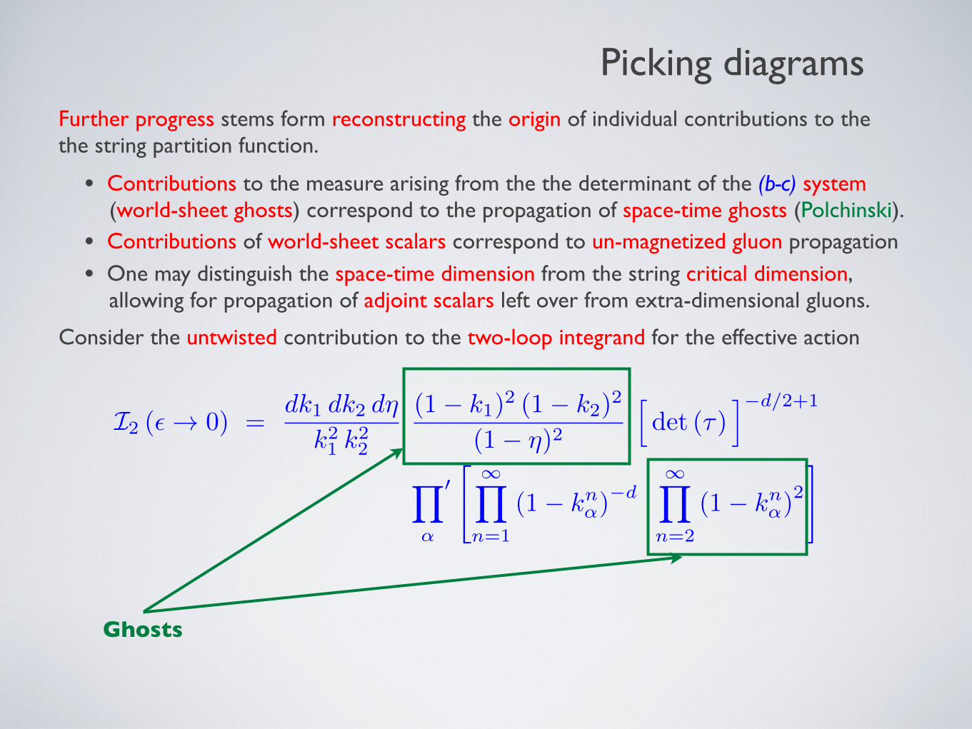
Further progress stems form reconstructing the origin of individual contributions to thethe string partition function.
• Contributions to the measure arising from the the determinant of the (b-c) system (world-sheet ghosts) correspond to the propagation of space-time ghosts (Polchinski).
• Contributions of world-sheet scalars correspond to un-magnetized gluon propagation
• One may distinguish the space-time dimension from the string critical dimension, allowing for propagation of adjoint scalars left over from extra-dimensional gluons.
Consider the untwisted contribution to the two-loop integrand for the effective action
Ghosts
Picking diagrams
I2 (✏ ! 0) =dk1 dk2 d⌘
k21 k22
(1� k1)2 (1� k2)2
(1� ⌘)2
hdet (⌧)
i�d/2+1
Y
↵
0" 1Y
n=1
(1� kn↵)�d
1Y
n=2
(1� kn↵)2
#
Further progress stems form reconstructing the origin of individual contributions to thethe string partition function.
• Contributions to the measure arising from the the determinant of the (b-c) system (world-sheet ghosts) correspond to the propagation of space-time ghosts (Polchinski).
• Contributions of world-sheet scalars correspond to un-magnetized gluon propagation
• One may distinguish the space-time dimension from the string critical dimension, allowing for propagation of adjoint scalars left over from extra-dimensional gluons.
Consider the untwisted contribution to the two-loop integrand for the effective action
Ghosts
Un-magnetized gluons
Picking diagrams
I2 (✏ ! 0) =dk1 dk2 d⌘
k21 k22
(1� k1)2 (1� k2)2
(1� ⌘)2
hdet (⌧)
i�d/2+1
Y
↵
0" 1Y
n=1
(1� kn↵)�d
1Y
n=2
(1� kn↵)2
#

Further progress stems form reconstructing the origin of individual contributions to thethe string partition function.
• Contributions to the measure arising from the the determinant of the (b-c) system (world-sheet ghosts) correspond to the propagation of space-time ghosts (Polchinski).
• Contributions of world-sheet scalars correspond to un-magnetized gluon propagation
• One may distinguish the space-time dimension from the string critical dimension, allowing for propagation of adjoint scalars left over from extra-dimensional gluons.
Consider the untwisted contribution to the two-loop integrand for the effective action
d = 4 - 2 ε Ghosts
Un-magnetized gluons
Picking diagrams
I2 (✏ ! 0) =dk1 dk2 d⌘
k21 k22
(1� k1)2 (1� k2)2
(1� ⌘)2
hdet (⌧)
i�d/2+1
Y
↵
0" 1Y
n=1
(1� kn↵)�d
1Y
n=2
(1� kn↵)2
#
Further progress stems form reconstructing the origin of individual contributions to thethe string partition function.
• Contributions to the measure arising from the the determinant of the (b-c) system (world-sheet ghosts) correspond to the propagation of space-time ghosts (Polchinski).
• Contributions of world-sheet scalars correspond to un-magnetized gluon propagation
• One may distinguish the space-time dimension from the string critical dimension, allowing for propagation of adjoint scalars left over from extra-dimensional gluons.
Consider the untwisted contribution to the two-loop integrand for the effective action
d = 4 - 2 ε Ghosts
Un-magnetized gluons d → D = d + s
Picking diagrams
I2 (✏ ! 0) =dk1 dk2 d⌘
k21 k22
(1� k1)2 (1� k2)2
(1� ⌘)2
hdet (⌧)
i�d/2+1
Y
↵
0" 1Y
n=1
(1� kn↵)�d
1Y
n=2
(1� kn↵)2
#
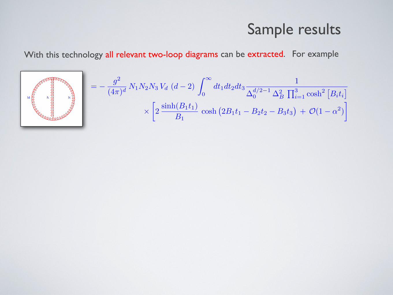
With this technology all relevant two-loop diagrams can be extracted. For example
Sample results
= � g2
(4⇡)dN1N2N3 Vd (d� 2)
Z 1
0dt1dt2dt3
1
�
d/2�10 �
2B
Q3i=1 cosh
2 ⇥Biti⇤
⇥2
sinh(B1t1)
B1cosh
�2B1t1 �B2t2 �B3t3
�+ O(1� ↵2
)
�

With this technology all relevant two-loop diagrams can be extracted. For example
• Isolating the four-point vertex requires integrating exactly over η after expanding in ki , discarding tachyon-related singularities.
Sample results
= � g2
(4⇡)dN1N2N3 Vd
1 + ↵2
2
Z 1
0dt1dt2
B1t1 B2t2sinh(B1t1) sinh(B2t2)
⇥h(d� 2) + 2 cosh
�2B1t1 + 2B2t2
�+ O(1� ↵2
)
i
= � g2
(4⇡)dN1N2N3 Vd (d� 2)
Z 1
0dt1dt2dt3
1
�
d/2�10 �
2B
Q3i=1 cosh
2 ⇥Biti⇤
⇥2
sinh(B1t1)
B1cosh
�2B1t1 �B2t2 �B3t3
�+ O(1� ↵2
)
�

With this technology all relevant two-loop diagrams can be extracted. For example
• Isolating the four-point vertex requires integrating exactly over η after expanding in ki , discarding tachyon-related singularities. Tests for ambiguities are underway.
Sample results
= � g2
(4⇡)dN1N2N3 Vd
1 + ↵2
2
Z 1
0dt1dt2
B1t1 B2t2sinh(B1t1) sinh(B2t2)
⇥h(d� 2) + 2 cosh
�2B1t1 + 2B2t2
�+ O(1� ↵2
)
i
= � g2
(4⇡)dN1N2N3 Vd (d� 2)
Z 1
0dt1dt2dt3
1
�
d/2�10 �
2B
Q3i=1 cosh
2 ⇥Biti⇤
⇥2
sinh(B1t1)
B1cosh
�2B1t1 �B2t2 �B3t3
�+ O(1� ↵2
)
�
Preliminary ...

With this technology all relevant two-loop diagrams can be extracted. For example
• Isolating the four-point vertex requires integrating exactly over η after expanding in ki , discarding tachyon-related singularities. Tests for ambiguities are underway.
• All Schwinger parameter integrands are reproduced by string theory with
Sample results
= � g2
(4⇡)dN1N2N3 Vd
1 + ↵2
2
Z 1
0dt1dt2
B1t1 B2t2sinh(B1t1) sinh(B2t2)
⇥h(d� 2) + 2 cosh
�2B1t1 + 2B2t2
�+ O(1� ↵2
)
i
= � g2
(4⇡)dN1N2N3 Vd (d� 2)
Z 1
0dt1dt2dt3
1
�
d/2�10 �
2B
Q3i=1 cosh
2 ⇥Biti⇤
⇥2
sinh(B1t1)
B1cosh
�2B1t1 �B2t2 �B3t3
�+ O(1� ↵2
)
�
Preliminary ...
↵ = 1
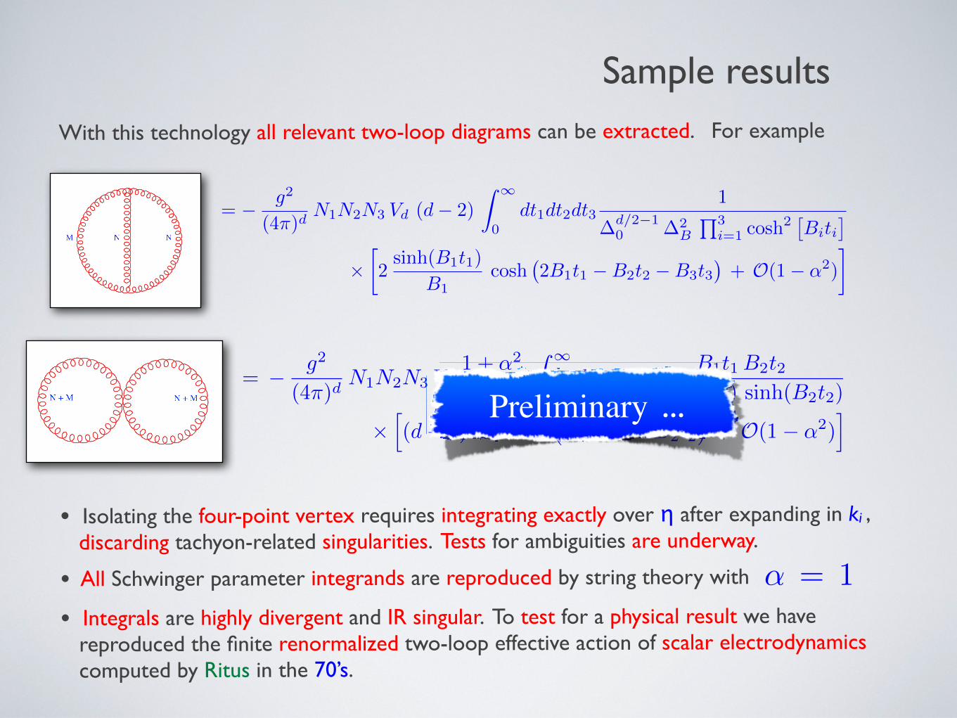
With this technology all relevant two-loop diagrams can be extracted. For example
• Isolating the four-point vertex requires integrating exactly over η after expanding in ki , discarding tachyon-related singularities. Tests for ambiguities are underway.
• All Schwinger parameter integrands are reproduced by string theory with
• Integrals are highly divergent and IR singular. To test for a physical result we have reproduced the finite renormalized two-loop effective action of scalar electrodynamics computed by Ritus in the 70’s.
Sample results
= � g2
(4⇡)dN1N2N3 Vd
1 + ↵2
2
Z 1
0dt1dt2
B1t1 B2t2sinh(B1t1) sinh(B2t2)
⇥h(d� 2) + 2 cosh
�2B1t1 + 2B2t2
�+ O(1� ↵2
)
i
= � g2
(4⇡)dN1N2N3 Vd (d� 2)
Z 1
0dt1dt2dt3
1
�
d/2�10 �
2B
Q3i=1 cosh
2 ⇥Biti⇤
⇥2
sinh(B1t1)
B1cosh
�2B1t1 �B2t2 �B3t3
�+ O(1� ↵2
)
�
Preliminary ...
↵ = 1

OUTLOOK
To summarize Our understanding of the field theory limit of perturbative string amplitudes grows at
widely separated time intervals.
Pushing beyond one loop and beyond the string ground state proved difficult so far.
Studying effective actions in constant background gauge fields at multiloops is now possible and useful to understand the fragmentation of moduli space in the field theory limit.
We have made significant progress.
• The proper variables to identify each vacuum bubble topology have been identified, in a manner generalizable to higher genera.
• Reconstructing the origin of each factor of the string partition function it is possible to identify not only individual topologies but individual diagrams.
• String theory naturally computes diagrams in a specific gauge: the Gervais- Neveu Background Field (GNBF) gauge with parameter α = 1. This applies to all genera.
Massless and massive scalar fields, massless gauge bosons and ghosts can be handled using the open bosonic string. Gravitons are expected to follow the same pattern in the closed string channel. Fermions must await further technical developments for superstring amplitudes.
Applications can be envisaged to perturbative dualities, non-perturbative field theory effects (D-branes and instantons), string phenomenology and further theory developments.

THANK YOU!