lorentz and semi-riemannian spaces with alexandrov curvature

communications in

analysis and geometry

Volume 16, Number 2, 251–282, 2008

Lorentz and semi-Riemannian spaces withAlexandrov curvature bounds

Stephanie B. Alexander and Richard L. Bishop

A semi-Riemannian manifold is said to satisfy R ≥ K (or R ≤ K)if spacelike sectional curvatures are ≥K and timelike ones are ≤K(or the reverse). Such spaces are abundant, as warped product con-structions show; they include, in particular, big bang Robertson–Walker spaces. By stability, there are many non-warped prod-uct examples. We prove the equivalence of this type of curvaturebound with local triangle comparisons on the signed lengths ofgeodesics. Specifically, R ≥ K if and only if locally the signedlength of the geodesic between two points on any geodesic triangleis at least that for the corresponding points of its model trianglein the Riemannian, Lorentz or anti-Riemannian plane of curva-ture K (and the reverse for R ≤ K). The proof is by compari-son of solutions of matrix Riccati equations for a modified shapeoperator that is smoothly defined along reparametrized geodesics(including null geodesics) radiating from a point. Also proved aresemi-Riemannian analogues to the three basic Alexandrov trianglelemmas, namely, the realizability, hinge and straightening lemmas.These analogues are intuitively surprising, both in one of the quan-tities considered, and also in the fact that monotonicity statementspersist even though the model space may change. Finally, the alge-braic meaning of these curvature bounds is elucidated, for example,by relating them to a curvature function on null sections.

1. Introduction

1.1. Main theorem

Alexandrov spaces are geodesic metric spaces with curvature bounds in thesense of local triangle comparisons. Specifically, let SK denote the sim-ply connected 2-dimensional Riemannian space form of constant curvatureK. For curvature bounded below (CBB) by K, the distance between anytwo points of a geodesic triangle is required to be more than or equal tothe distance between the corresponding points on the “model” triangle

251

252 Stephanie B. Alexander and Richard L. Bishop

with the same sidelengths in SK . For curvature bounded above (CBA),substitute “less than or equal to.” Examples of Alexandrov spaces includeRiemannian manifolds with sectional curvature ≥K or ≤K. A crucialproperty of Alexandrov spaces is their preservation by Gromov–Hausdorffconvergence (assuming uniform injectivity radius bounds in the CBA case).Moreover, CBB spaces are topologically stable in the limit [1], a fact atthe root of landmark Riemannian finiteness and recognition theorems. (SeeGrove’s essay [2].) CBA spaces are also important in geometric group theory(see [3, 4]) and harmonic map theory (see, e.g., [5–7]).

In Lorentzian geometry, timelike comparison and rigidity theory is welldeveloped. Early advances in timelike comparison geometry were made byFlaherty [8], Beem and Ehrlich [9], and Harris [10,11]. In particular, a purelytimelike, global triangle comparison theorem was proved by Harris [10].A major advance in rigidity theory was the Lorentzian splitting theorem,to which a number of researchers contributed; see the survey in [12], andalso the subsequent warped product splitting theorem in [13]. The com-parison theorems mentioned assume a bound on sectional curvatures K(P )of timelike 2-planes P . Note that a bound over all non-singular 2-planeforces the sectional curvature to be constant [14], and so such bounds areuninteresting.

This project began with the realization that certain Lorentzian warpedproducts, which may be called Minkowski, de Sitter, or anti-de Sitter cones,possess a global triangle comparison property that is not just timelike, butis fully analogous to the Alexandrov one. The comparisons we mean are onsigned lengths of geodesics, where the timelike sign is taken to be negative.In this paper, length of either geodesics or vectors is always signed, and wewill not talk about the length of non-geodesic curves. The model spaces areSK , MK , or −SK , where MK is the simply connected 2-dimensional Lorentzspace form of constant curvature K, and −SK is SK with the sign of themetric switched, a space of constant curvature −K.

The cones mentioned turn out to have sectional curvature bounds of thefollowing type. For any semi-Riemannian manifold, call a tangent sectionspacelike if the metric is definite there, and timelike if it is non-degenerateand indefinite. Write R ≥ K if spacelike sectional curvatures are ≥K andtimelike ones are ≤K; for R ≤ K, reverse “timelike” and “spacelike.” Equiv-alently, R ≥ K if the curvature tensor satisfies

(1.1) R(v, w, v, w) ≥ K(〈v, v〉〈w, w〉 − 〈v, w〉2),

and similarly with inequalities reversed.

Lorentz and semi-Riemannian spaces 253

The meaning of this type of curvature bound is clarified by noting thatif one has merely a bound above on timelike sectional curvatures, or merelya bound below on spacelike ones, then the restriction RV of the sectionalcurvature function to any non-degenerate 3-plane V has a curvature boundbelow in our sense: RV ≥ K(V ) (as follows from [15]; see our Section 6).Then R ≥ K means that K(V ) may be chosen independently of V .

Spaces satisfying R ≥ K (or R ≤ K) are abundant, as warped productconstructions show. They include, for example, the big bang cosmologicalmodels discussed by Hawking and Ellis [16, pp. 134–138] (see our Section 7).Since there are many warped product examples satisfying R ≥ K for all Kin a non-trivial finite interval, then by stability, there are many non-warpedproduct examples.

Searching the literature for this type of curvature bound, we found it hadbeen studied earlier by Andersson and Howard [17]. Their paper contains aRiccati equation analysis and gap rigidity theorems. For example: a geodesi-cally complete semi-Riemannian manifold of dimension n ≥ 3 and index k,having either R ≥ 0 or R ≤ 0 and an end with finite fundamental group onwhich R ≡ 0, is Rn

k [17]. Their method uses parallel hypersurfaces, and doesnot concern triangle comparisons or the methods of Alexandrov geometry.Subsequently, Dıaz–Ramos, Garcıa–Rıo, and Hervella obtained a volumecomparison theorem for “celestial spheres” (exponential images of spheresin spacelike hyperplanes) in a Lorentz manifold with R ≥ K or R ≤ K [18].

Does this type of curvature bound always imply local triangle compar-isons, or do triangle comparisons only arise in special cones? In this paperwe prove that curvature bounds R ≥ K or R ≤ K are actually equivalent tolocal triangle comparisons. The existence of model triangles is described inthe realizability lemma of Section 2. It states that any point in R3 − (0, 0, 0)represents the sidelengths of a unique triangle in a model space of curvature0, and the same holds for K �= 0 under appropriate size bounds for K.

We say U is a normal neighborhood if it is a normal coordinate neigh-borhood (the diffeomeorphic exponential image of some open domain inthe tangent space) of each of its points. There is a corresponding distin-guished geodesic between any two points of U , and the following theoremrefers to these geodesics and the triangles they form. If in addition thetriangles satisfy size bounds for K, we say U is normal for K. All geodesicsare assumed parametrized by [0, 1], and by corresponding points on twogeodesics, we mean points having the same affine parameter.

Theorem 1.1. If a semi-Riemannian manifold satisfies R ≥ K (R ≤ K),and U is a normal neighborhood for K, then the signed length of the geodesic


between two points on any geodesic triangle of U is at least (at most) thatfor the corresponding points on the model triangle in SK , MK or −SK .

Conversely, if triangle comparisons hold in some normal neighborhoodof each point of a semi-Riemannian manifold, then R ≥ K (R ≤ K).

In this paper, we restrict our attention to local triangle comparisons (i.e.,to normal neighborhoods) in smooth spaces. In the Riemannian/Alexandrovtheory, local triangle comparisons have features of potential interest tosemi-Riemannian and Lorentz geometers: they incorporate singularities,imply global comparison theorems, and are consistent with a theory oflimit spaces [4, 25–27]. Our longer-term goal is to see what the extensionof the theory presented here can contribute to similar questions in semi-Riemannian and Lorentz geometry.

1.2. Approach

We begin by mentioning some intuitive barriers to approaching Theorem1.1. In resolving them, we are going to draw on papers by Karcher [19]and Andersson and Howard [17], putting them to different uses than wereoriginally envisioned.

First, a fundamental object in Riemannian theory is the locally isomet-rically embedded interval, that is, the unitspeed geodesic. These are thepaths studied in [19] and [17]. However, in the semi-Riemannian case thischoice constrains consideration to fields of geodesics all having the samecausal character. By contrast, our construction, which uses affine parame-ters on [0, 1], applies uniformly to all the geodesics radiating from a point(or orthogonally from a non-degenerate submanifold).

Secondly, a common paradigm in Riemannian and Alexandrov compar-ison theory is the construction of a curve that is shorter than some originalone, so that the minimizing geodesic between the endpoints is even shorter.In the Lorentz setting, this argument still works for timelike curves, undera causality assumption. However, spacelike geodesics are unstable criticalpoints of the length functional, and so this argument is forbidden.

Third, while the comparisons we seek can be reduced in the Riemanniansetting to 1-dimensional Riccati equations (as in [19]), the semi-Riemanniancase seems to require matrix Riccati equations (as in [17]). Such increasedcomplexity is to be expected, since semi-Riemannian curvature bounds below(say) have some of the qualities of Riemannian curvature bounds both belowand above.


Let us start by outlining Karcher’s approach to Riemannian curvaturebounds. It included a new proof of local triangle comparisons, one that inte-grated infinitesimal Rauch comparisons to get distance comparisons withoutusing the “forbidden argument” mentioned before. Such an approach, moti-vated by simplicity rather than necessity in the Riemannian case, is whatthe semi-Riemannian case requires.

In this approach, Alexandrov curvature bounds are characterized by adifferential inequality. Namely, M has CBB by K in the triangle comparisonsense if and only if for every q ∈ M and unit-speed geodesic γ, the differentialinequality

(1.2) (f ◦ γ)′′ + Kf ◦ γ ≤ 1

is satisfied (in the barrier sense) by the following function f = mdK dq:

(1.3) mdK dq =

⎧⎪⎨

⎪⎩

(1/K)(1 − cosh√

−Kdq), K < 0(1/K)(1 − cos

√Kdq), K > 0

d2q/2, K = 0.

The reason for this equivalence is that the inequalities (1.2) reduce toequations in the model spaces SK ; since solutions of the differential inequal-ities may be compared with those of the equations, distances in M may becompared with those in SK . The functions mdK dq then provide a conve-nient connection between triangle comparisons and curvature bounds, sincethey lead via their Hessians to a Riccati equation along radial geodesicsfrom q.

We wish to view this program as a special case of a procedure on semi-Riemannian manifolds. For a geodesic γ parametrized by [0, 1], let

(1.4) E(γ) = 〈γ′(0), γ′(0)〉.

Thus E(γ) = ±|γ|2. In this paper, we work with normal neighborhoods, andset E(p, q) = E(γpq) where γpq is the geodesic from p to q that is distin-guished by the normal neighborhood.

(In a broader setting, one may instead use the definition

(1.5) E(p, q) = Eq(p) = inf{E(γ) : γ is a geodesic joining p and q},

under hypotheses that ensure the two definitions agree locally. In (1.5),E(p, q) = ∞ if p and q are not connected by a geodesic.)


Now define the modified distance function hK,q at q by

(1.6) hK,q =

{(1 − cos

√KEq)/K =

∑∞n=1

(−K)n−1(Eq)n

(2n)! , K �= 0

Eq/2, K = 0.

Here, the formula remains valid when the argument of cosine is imagi-nary, converting cos to cosh. In the Riemannian case, hK,q = mdK dq. TheCBB triangle comparisons we seek will be characterized by the differentialinequality

(1.7) (hK,q ◦ γ)′′ + KE(γ)hK,q ◦ γ ≤ E(γ),

on any geodesic γ parametrized by [0, 1].The self-adjoint operator S = SK,q associated with the Hessian of hK,q

may be regarded as a modified shape operator. It has the following properties:in the model spaces, it is a scalar multiple of the identity on the tangentspace to M at each point; along a non-null geodesic from q, its restrictionto normal vectors is a scalar multiple of the second fundamental form of theequidistant hypersurfaces from q; it is smoothly defined on the regular set ofEq, hence along null geodesics from q (as the second fundamental forms arenot); and finally, it satisfies a matrix Riccati equation along every geodesicfrom q, after reparametrization as an integral curve of gradhK,q.

We shall also need semi-Riemannian analogues to the three basic trianglelemmas on which Alexandrov geometry builds, namely, the realizability,hinge and straightening lemmas. The analogues are intuitively surprising,both in one of the quantities considered, and also in the fact that mono-tonicity statements persist even though the model space may change. Thestraightening lemma is an indicator that, as in the standard Riemannian/Alexandrov case, there is a singular counterpart to the smooth theory devel-oped in this paper.

1.3. Outline of paper

We begin in Section 2 with the triangle lemmas just mentioned. In Section 3,it is shown that the differential inequalities (1.7) become equations in themodel spaces, and hence characterize our triangle comparisons.

Comparisons for the modified shape operators under semi-Riemanniancurvature bounds are proved in Section 4, and Theorem 1.1 is proved inSection 5. In Section 6, semi-Riemannian curvature bounds are related


to the analysis by Beem and Parker of the pointwise ranges of sectionalcurvature [15], and to the “null” curvature bounds considered by Uhlenbeck[20] and Harris [10]. Finally, Section 7 considers examples of semi-Riemannianspaces with curvature bounds, including Robertson–Walker “big bang”spacetimes.

2. Triangle lemmas in model spaces

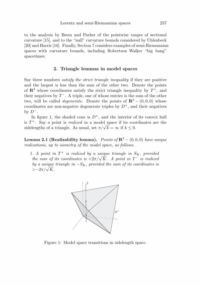
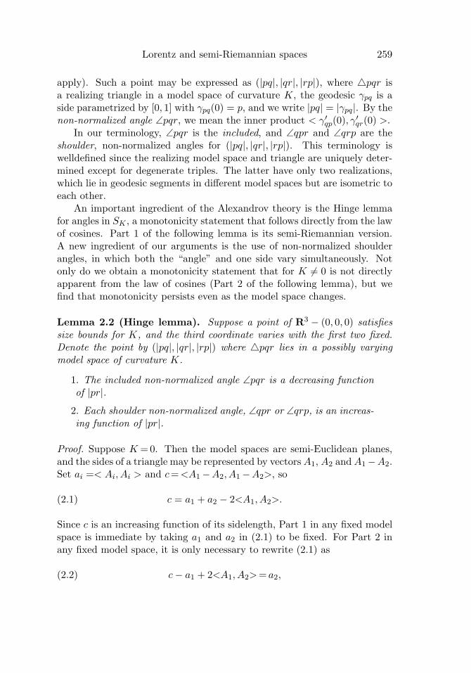
Say three numbers satisfy the strict triangle inequality if they are positiveand the largest is less than the sum of the other two. Denote the pointsof R3 whose coordinates satisfy the strict triangle inequality by T+, andtheir negatives by T−. A triple, one of whose entries is the sum of the othertwo, will be called degenerate. Denote the points of R3 − (0, 0, 0) whosecoordinates are non-negative degenerate triples by D+, and their negativesby D−.

In figure 1, the shaded cone is D+, and the interior of its convex hullis T+. Say a point is realized in a model space if its coordinates are thesidelengths of a triangle. As usual, set π/

√k = ∞ if k ≤ 0.

Lemma 2.1 (Realizability lemma). Points of R3 − (0, 0, 0) have uniquerealizations, up to isometry of the model space, as follows.

1. A point in T+ is realized by a unique triangle in SK , providedthe sum of its coordinates is <2π/

√K. A point in T− is realized

by a unique triangle in −SK , provided the sum of its coordinates is>−2π/

√K.

L

D+

Figure 1: Model space transitions in sidelength space.


2. A point in D+ is realized by unique triangles in SK and MK ,provided the largest coordinate is <π/

√K. A point in D− is real-

ized by unique triangles in −SK and MK , provided the smallestcoordinate is >−π/

√K.

3. A point in the complement of T+ ∪ T− ∪ D+ ∪ D− ∪ (0, 0, 0) isrealized by a unique triangle in M0 = R2

1. For K > 0, if the largestcoordinate is <π/

√K, the point is realized by a unique triangle in

MK . For K < 0, if the smallest coordinate is >−π/√

−K, the pointis realized by a unique triangle in MK .

Proof. Part 1 is standard, as is Part 2 for ±SK . Now consider a point notin T+ ∪ T− ∪ (0, 0, 0), and denote its coordinates by a ≥ b ≥ c.

To realize this point in M0 = R21, suppose a > 0 and take a segment γ of

length a on the x1-axis. Since distance “circles” about a point p are pairs oflines of slope ±1 through p if the radius is 0, and hyperbolas asymptotic tothese lines otherwise, it is easy to see that circles about the endpoints of γintersect, either in two points or tangentially, subject only to the conditionthat a ≥ b + c if c ≥ 0, namely, the point is not in T+. Thus our point maybe realized in R2

1, uniquely up to an isometry of R21. On the other hand, if

a ≤ 0 then c < 0, so by switching the sign of the metric, we have just shownthere is a realization in −R2

1 = R21.

For K > 0, MK is the simply connected cover of the quadric surface< p, p >= 1/K in Minkowski 3-space with signature (+ + −). Suppose0 < a < π/

√K, and take a segment γ of length a on the quadric’s equa-

torial circle of length 2π/√

K in the x1x2-plane. A distance circle aboutan endpoint of γ is a hyperbola or pair of lines obtained by intersectionwith a 2-plane parallel to or coinciding with the tangent plane. Two circlesabout the endpoints of γ intersect, either in two points or tangentially, if thevertical line of intersection of their 2-planes cuts the quadric. This occurssubject only to the condition that a ≥ b + c if c ≥ 0, namely, the point isnot in T+. On the other hand, if a ≤ 0 then c < 0. Take a segment γ oflength c in the quadric, where γ is symmetric about the x1x2-plane. Circlesof non-positive radius about the endpoints of γ intersect if the horizontalline of intersection of their 2-planes cuts the quadric, and this occurs subjectonly to the condition that c < a + b, namely, the point is not in T−.

Since M−K = −MK , switching the sign of the metric completes theproof. �

Let us say the points of R3 − (0, 0, 0) for which Lemma 2.1 gives modelspace realizations satisfy size bounds for K (for K = 0, no size bounds


apply). Such a point may be expressed as (|pq|, |qr|, |rp|), where pqr isa realizing triangle in a model space of curvature K, the geodesic γpq is aside parametrized by [0, 1] with γpq(0) = p, and we write |pq| = |γpq|. By thenon-normalized angle ∠pqr, we mean the inner product < γ′

qp(0), γ′qr(0) >.

In our terminology, ∠pqr is the included, and ∠qpr and ∠qrp are theshoulder, non-normalized angles for (|pq|, |qr|, |rp|). This terminology iswelldefined since the realizing model space and triangle are uniquely deter-mined except for degenerate triples. The latter have only two realizations,which lie in geodesic segments in different model spaces but are isometric toeach other.

An important ingredient of the Alexandrov theory is the Hinge lemmafor angles in SK , a monotonicity statement that follows directly from the lawof cosines. Part 1 of the following lemma is its semi-Riemannian version.A new ingredient of our arguments is the use of non-normalized shoulderangles, in which both the “angle” and one side vary simultaneously. Notonly do we obtain a monotonicity statement that for K �= 0 is not directlyapparent from the law of cosines (Part 2 of the following lemma), but wefind that monotonicity persists even as the model space changes.

Lemma 2.2 (Hinge lemma). Suppose a point of R3 − (0, 0, 0) satisfiessize bounds for K, and the third coordinate varies with the first two fixed.Denote the point by (|pq|, |qr|, |rp|) where pqr lies in a possibly varyingmodel space of curvature K.

1. The included non-normalized angle ∠pqr is a decreasing functionof |pr|.

2. Each shoulder non-normalized angle, ∠qpr or ∠qrp, is an increas-ing function of |pr|.

Proof. Suppose K = 0. Then the model spaces are semi-Euclidean planes,and the sides of a triangle may be represented by vectors A1, A2 and A1 −A2.Set ai =< Ai, Ai > and c = <A1 −A2, A1 −A2>, so

(2.1) c = a1 + a2 − 2<A1, A2>.

Since c is an increasing function of its sidelength, Part 1 in any fixed modelspace is immediate by taking a1 and a2 in (2.1) to be fixed. For Part 2 inany fixed model space, it is only necessary to rewrite (2.1) as

(2.2) c − a1 + 2<A1, A2> = a2,


where a1 and c are fixed.A change of model space occurs when the varying point in R3 − (0, 0, 0)

moves upward on a vertical line L, and passes either into or out of T+ bycrossing D+ (the same argument will hold for T− and D−). See figure 1.Thus L is the union of three closed segments, intersecting only at theirtwo endpoints on D+. We have just seen that the included angle func-tion is decreasing on each segment, since the realizing triangles are in thesame model space (by choice at the endpoints and by necessity elsewhere).Since the values at the endpoints are the same from left or right, the includedangle function is decreasing on all of L. Similarly, each shoulder angle func-tion is increasing.

Suppose K > 0. The vertices of a triangle in the quadric model spaceare also the vertices of a triangle in an ambient 2-plane, whose sides arethe chords of the original sides. The length of the chord is an increasingfunction of the original sidelength. Thus to derive the lemma for K > 0from (2.1) and (2.2), we must verify the following: if a triangle in a quadricmodel space varies with fixed sidelengths adjacent to one vertex, and v1, v2are the tangent vectors to the sides at that vertex, then < v1, v2 > is anincreasing function of < A1, A2 > where the Ai are the chordal vectors ofthe two sides. Indeed, all points of a distance circle of non-zero radius inthe quadric model space lie at a fixed non-zero ambient distance from thetangent plane at the centerpoint. Thus Ai is a linear combination of vi anda fixed normal vector N to the tangent plane, where the coefficients dependonly on the sidelength �i. The desired correlation follows.

By switching the sign of the metric, we obtain the claim for K < 0. �

Remark 2.3. The Law of Cosines in a semi-Riemannian model space withK = 0 is (2.1). If K �= 0, the Law of Cosines for pqr may be written inunified form as follows:

cos√

KE(γpr) = cos√

KE(γpq) cos√

KE(γqr)(2.3)

− K∠pqrsin

√KE(γpq)

√KE(γpq)

sin√

KE(γqr)√

KE(γqr).

Here we assume pqr satisfies the size bounds for K. Then each sidelengthis < π/

√K if K > 0, and > −π/

√−K if K < 0. Part 1 of Lemma 2.2 can

be derived from (2.3) as follows. Fix E(γpq) and E(γqr), and observe thatcos

√Kc is decreasing in c if K > 0, regardless of the sign of c and even as c

passes through 0, and increasing in c if K < 0. The size bounds imply that

lorentz and semi-riemannian spaces with alexandrov curvature

Documents