Loopy Belief Propagation:

Convergence and Effects of Message Errors

Alexander T. Ihler, John W. Fisher III, and Alan S. Willsky

Initial version June, 2004; Last revised April, 2005

LIDS Technical Report # 2602(corrected version)

Abstract

Belief propagation (BP) is an increasingly popular method of performing approximate in-ference on arbitrary graphical models. At times, even further approximations are required,whether due to quantization of the messages or model parameters, from other simplified mes-sage or model representations, or from stochastic approximation methods. The introduction ofsuch errors into the BP message computations has the potential to affect the solution obtainedadversely. We analyze the effect resulting from message approximation under two particularmeasures of error, and show bounds on the accumulation of errors in the system. This analysisleads to convergence conditions for traditional BP message passing, and both strict bounds andestimates of the resulting error in systems of approximate BP message passing.

1 Introduction

Graphical models and message-passing algorithms defined on graphs comprise a growing field ofresearch. In particular, the belief propagation (or sum-product) algorithm has become a popularmeans of solving inference problems exactly or approximately. One part of its appeal lies in itsoptimality for tree-structured graphical models (models which contain no loops). However, its isalso widely applied to graphical models with cycles. In these cases it may not converge, and if itdoes its solution is approximate; however in practice these approximations are often good. Recently,some additional justifications for loopy belief propagation have been developed, including a handfulof convergence results for graphs with cycles [1, 2, 3].

The approximate nature of loopy belief propagation is often a more than acceptable price forperforming efficient inference; in fact, it is sometimes desirable to make additional approximations.There may be a number of reasons for this—for example, when exact message representation is com-putationally intractable, the messages may be approximated stochastically [4] or deterministicallyby discarding low-likelihood states [5]. For belief propagation involving continuous, non-Gaussianpotentials, some form of approximation is required to obtain a finite parameterization for the mes-sages [6, 7, 8]. Additionally, simplification of complex graphical models through edge removal,quantization of the potential functions, or other forms of distributional approximation may be con-sidered in this framework. Finally, one may wish to approximate the messages and reduce theirrepresentation size for another reason—to decrease the communications required for distributedinference applications. In distributed message passing, one may approximate the transmitted mes-sage to reduce its representational cost [9], or discard it entirely if it is deemed “sufficiently similar”to the previously sent version [10]. Through such means one may significantly reduce the amountof communications required.

Given that message approximation may be desirable, we would like to know what effect theerrors introduced have on our overall solution. In order to characterize the approximation effects

1

in graphs with cycles, we analyze the deviation from the solution given by “exact” loopy beliefpropagation (not, as is typically considered, the deviation of loopy BP from the true marginaldistributions). As a byproduct of this analysis, we also obtain some results on the convergence ofloopy belief propagation.

We begin in Section 2 by briefly reviewing the relevant details of graphical models and beliefpropagation. Section 4 then examines the consequences of measuring a message error by its dy-namic range. In particular, we explain the utility of this measure and its behavior with respectto the operations of belief propagation. This allows us to derive conditions for the convergenceof traditional loopy belief propagation, and bounds on the distance between any pair of BP fixedpoints (Sections 5.1-5.2), and these results are easily extended to many approximate forms of BP(Section 5.3). If the errors introduced are independent (a typical assumption in, for example, quan-tization analysis [11, 12]), tighter estimates of the resulting error can be obtained (Section 5.5).

It is also instructive to examine other measures of message error, in particular ones whichemphasize more average-case (as opposed to pointwise or worst-case) differences. To this end, weconsider a KL-divergence based measure in Section 6. While the analysis of the KL-divergencemeasure is considerably more difficult and does not lead to strict guarantees, it serves to give someintuition into the behavior of perturbed BP under an average-case difference measure.

2 Graphical Models

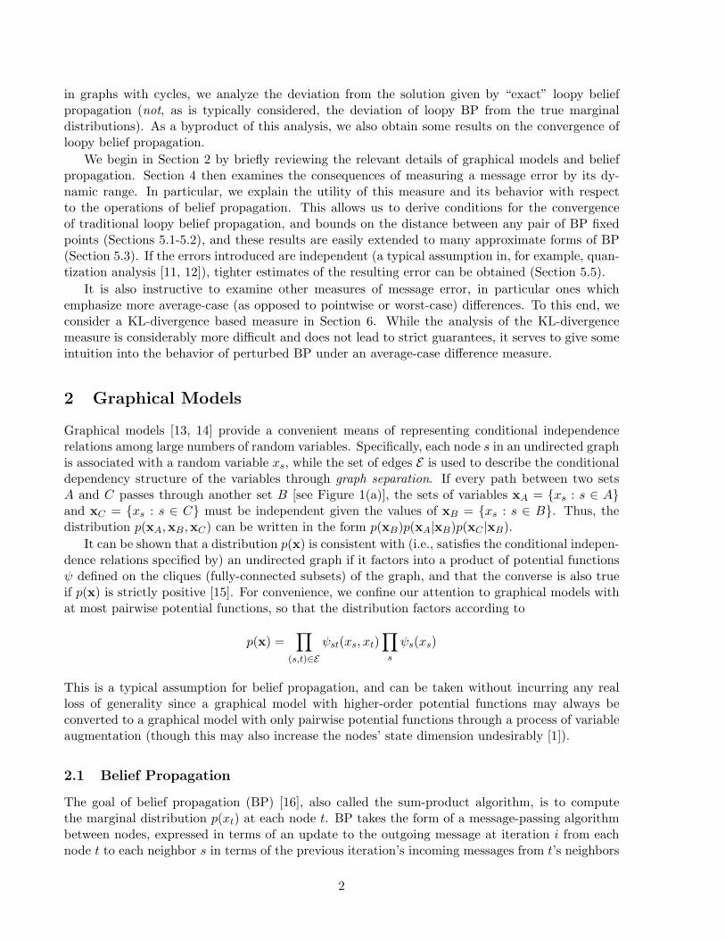
Graphical models [13, 14] provide a convenient means of representing conditional independencerelations among large numbers of random variables. Specifically, each node s in an undirected graphis associated with a random variable xs, while the set of edges E is used to describe the conditionaldependency structure of the variables through graph separation. If every path between two setsA and C passes through another set B [see Figure 1(a)], the sets of variables xA = {xs : s ∈ A}and xC = {xs : s ∈ C} must be independent given the values of xB = {xs : s ∈ B}. Thus, thedistribution p(xA,xB,xC) can be written in the form p(xB)p(xA|xB)p(xC |xB).

It can be shown that a distribution p(x) is consistent with (i.e., satisfies the conditional indepen-dence relations specified by) an undirected graph if it factors into a product of potential functionsψ defined on the cliques (fully-connected subsets) of the graph, and that the converse is also trueif p(x) is strictly positive [15]. For convenience, we confine our attention to graphical models withat most pairwise potential functions, so that the distribution factors according to

p(x) =∏

(s,t)∈Eψst(xs, xt)

∏s

ψs(xs)

This is a typical assumption for belief propagation, and can be taken without incurring any realloss of generality since a graphical model with higher-order potential functions may always beconverted to a graphical model with only pairwise potential functions through a process of variableaugmentation (though this may also increase the nodes’ state dimension undesirably [1]).

2.1 Belief Propagation

The goal of belief propagation (BP) [16], also called the sum-product algorithm, is to computethe marginal distribution p(xt) at each node t. BP takes the form of a message-passing algorithmbetween nodes, expressed in terms of an update to the outgoing message at iteration i from eachnode t to each neighbor s in terms of the previous iteration’s incoming messages from t’s neighbors

2

u

u

u

t s

1

2

3

1 1

1 1 1 1

22

2

2

33

3

44

4

3 4

(a) (b) (c)

Figure 1: (a) Graphical models describe statistical dependency; here, the sets A and C are independentgiven B. (b) BP propagates information from t and its neighbors ui is to s by a simple message-passingprocedure; this procedure is exact on a tree, but approximate in graphs with cycles. (c) For a graph withcycles, one may show an equivalence between n iterations of loopy BP and the depth-n computation tree(shown here for n = 3 and rooted at node 1; example from [2]).

Γt [see Figure 1(b)],

mits(xs) ∝

∫ψts(xt, xs)ψt(xt)

∏

u∈Γt\smi−1

ut (xt)dxt (1)

Typically each message is normalized so as to integrate to unity (and we assume that such normal-ization is possible). For discrete-valued random variables, of course, the integral is replaced by asummation. At any iteration, one may calculate the belief at node t by

M it (xt) ∝ ψt(xt)

∏

u∈Γt

miut(xt) (2)

For tree-structured graphical models, belief propagation can be used to efficiently perform exactmarginalization. Specifically, the iteration (1) converges in a finite number of iterations (at mostthe length of the longest path in the graph), after which the belief (2) equals the correct marginalp(xt). However, as observed by [16], one may also apply belief propagation to arbitrary graphicalmodels by following the same local message passing rules at each node and ignoring the presenceof cycles in the graph; this procedure is typically referred to as “loopy” BP.

For loopy BP, the sequence of messages defined by (1) is not guaranteed to converge to a fixedpoint after any number of iterations. Under relatively mild conditions, one may guarantee theexistence of fixed points [17]. However, they may not be unique, nor are the results exact (thebelief M i

t does not converge to the true marginal p(xt)). In practice however the procedure oftenarrives at a reasonable set of approximations to the correct marginal distributions.

2.2 Computation Trees

It is sometimes convenient to think of loopy BP in terms of its computation tree. Tatikonda andJordan [2] showed that the effect of n iterations of loopy BP at any particular node s is equivalentto exact inference on a tree-structured ‘unrolling” of the graph from s. A small graph, and itsassociated 4-level computation tree rooted at node 1, are shown in Figure 1(c).

The computation tree with depth n consists of all length-n paths emanating from s in theoriginal graph which do not immediately backtrack (though they may eventually repeat nodes).1

We draw the computation tree as consisting of a number of levels, corresponding to each node inthe tree’s distance from the root, with the root node at level 0 and the leaf nodes at level n. Eachlevel may contain multiple replicas of each node, and thus there are potentially many replicas of

1Thus in Figure 1(c), the computation tree includes the sequence 1− 2− 4− 1, but not the sequence 1− 2− 4− 2.

3

each node in the graph. The root node s has replicas of all neighbors Γs in the original graph aschildren, while all other nodes have replicas of all neighbors except their parent node as children.

Each edge in the computation tree corresponds to both an edge in the original graph and aniteration in the BP message-passing algorithm. Specifically, assume an equivalent initialization ofboth the loopy graph and computation tree—i.e., the initial messages m0

ut in the loopy graph aretaken as inputs to the leaf nodes. Then, the upward messages from level n to level n − 1 matchthe messages m1

ut in the first iteration of loopy BP, and more generally, a upward message miut on

the computation tree which originates from a node u on level n− i + 1 to its parent node t on leveln − i is identical to the message from node u to node t in the ith iteration of loopy BP (out ofn total iterations) on the original graph. Thus, the incoming messages to the root node (level 0)correspond to the messages in the nth iteration of loopy BP.

2.3 Message Approximations

Let us now consider the concept of approximate BP messages. We begin by assuming that the “true”messages mts(xs) are some fixed point of BP, so that mi

ts = mi+1ts . We may ask what happens when

these messages are perturbed by some (perhaps small) error function ets(xs). Although there arecertainly other possibilities, the fact that BP messages are combined by taking their product makesit natural to consider multiplicative message deviations (or additive in the log-domain):

mits(xs) = mts(xs)ei

ts(xs)

To facilitate our analysis, we split the message update operation (1) into two parts. In the first,we focus on the message products

M its(xt) ∝ ψt(xt)

∏

u∈Γt\smi

ut(xt) M it (xt) ∝ ψt(xt)

∏

u∈Γt

miut(xt) (3)

where the proportionality constant is chosen to normalize M . The second operation, then, is themessage convolution

mi+1ts (xs) ∝

∫ψts(xs, xt)M i

ts(xt)dxt (4)

where again M is a normalized message or product of messages.In this paper, we use the convention that lowercase quantities (mts, ets, . . .) refer to messages

and message errors, while uppercase ones (Mts, Ets,Mt, . . .) refer to their products—at node t,the product of all incoming messages and the local potential is denoted Mt(xt), its approximationMt(xt) = Mt(xt)Et(xt), with similar definitions for Mts, Mts, and Ets.

3 Overview of Results

To orient the reader, we lay out the order and general results which are obtained in this paper.We begin in Section 4 by examining a dynamic range measure d (e) of the variability of a messageerror e(x) (or more generally of any function) and show how this measure behaves with respect tothe BP equations (1) and (2). Specifically, we show in Section 4.2 that the measure log d (e) is sub-additive with respect to the product operation (3), and contractive with respect to the convolutionoperation (4).

4

Applying these results to traditional belief propagation results in a new sufficient condition forBP convergence (Section 5.1), specifically

maxs,t

∑

u∈Γt\s

d (ψut)2 − 1

d (ψut)2 + 1

< 1; (5)

and this condition may be further improved in many cases. The condition (5) can be shown to beslightly stronger than the sufficient condition given in [2], and empirically appears to be strongerthan that of [3]. In experiments, the condition appears to be tight (exactly predicting uniqueness ornon-uniqueness of fixed points) for at least some problems, such as binary–valued random variables.More importantly, however, the method in which it is derived allows us to generalize to many othersituations:

1. Using the same methodology, we may demonstrate that any two BP fixed points must bewithin a ball of a calculable diameter; the condition (5) is equivalent to this diameter beingzero (Section 5.2).

2. Both the diameter of the bounding ball and the convergence criterion (5) are easily improvedfor graphical models with irregular geometry or potential strengths, leading to better condi-tions on graphs which are more “tree-like” (Section 5.3).

3. The same analysis may also be applied to the case of quantized or otherwise approximatedmessages and models (potential functions), yielding bounds on the resulting error (Sec-tion 5.4).

4. If we regard the message errors as a stochastic process, a similar analysis with a few additional,intuitive assumptions gives alternate, tighter estimates (though not necessarily bounds) ofperformance (Section 5.5).

Finally, in Section 6 we perform the same analysis for a less strict measure of message error (i.e.disagreement between a message m(x) and its approximation m(x)), namely the Kullback-Leiblerdivergence. This analysis shows that, while failing to provide strict bounds in several key ways,one is still able to obtain some intuition into the behavior of approximate message passing underan average-case difference measure.

In the next few sections, we first describe the dynamic range measure and discuss some of itssalient properties (Section 4). We then apply these properties to analyze the behavior of loopybelief propagation (Section 5). Almost all proofs are given in an in-line fashion, as they frequentlyserve to give intuition into the method and meaning of each result.

4 Dynamic Range Measure

In order to discuss the effects and propagation of errors, we first require a measure of the differencebetween two messages. In this section, we examine the following measure on ets(xs): let d (ets)denote the function’s dynamic range2, specifically

d (ets) = supa,b

√ets(a)/ets(b) (6)

2This measure has also been independently investigated to provide a stability analysis for the max-product algo-rithm in Bayes’ nets (acyclic, directed graphical models) [18]. While similar in some ways, the analysis for acyclicgraphs is considerably simpler; loopy graphs require demonstrating a rate of contraction, which we show is possiblefor the sum-product algorithm (Theorem 4.4).

5

m(x)

m(x) }}

0

log d (e)αmin

log m/m

(a) (b)

Figure 2: (a) A message m(x) and an example approximation m(x); (b) their log-ratiolog m(x)/m(x), and the error measure log d (e).

Then, we have that mts ≡ mts (i.e., the pointwise equality condition mts(x) = mts(x)∀x) if andonly if log d (ets) = 0. Figure 2 shows an example of m(x) and m(x) along with their associatederror e(x).

4.1 Motivation

We begin with a brief motivation for this choice of error measure. It has a number of desirablefeatures; for example, it is directly related to the pointwise log error between the two distributions.

Lemma 4.1. The dynamic range measure (6) may be equivalently defined by

log d (ets) = infα

supx| log αmts(x)− log mts(x)| = inf

αsup

x| log α− log ets(x)|

Proof. The minimum is given by log α = 12(supa log ets(a)+ infb log ets(b)), and thus the right-hand

side is equal to 12(supa log ets(a)− infb log ets(b)), or 1

2(supa,b log ets(a)/ets(b)), which by definitionis log d (ets).

The scalar α serves the purpose of “zero-centering” the function log ets(x) and making themeasure invariant to simple rescaling. This invariance reflects the fact that the scale factor forBP messages is essentially arbitrary, defining a class of equivalent messages. Although the scalefactor cannot be completely ignored, it takes on the role of a nuisance parameter. The inclusionof α in the definition of Lemma 4.1 acts to select particular elements of the equivalence classes(with respect to rescaling) from which to measure distance—specifically, choosing the closest suchmessages in a log-error sense. The log-error, dynamic range, and the minimizing α are depicted inFigure 2.

Lemma 4.1 allows the dynamic range measure to be related directly to an approximation errorin the log-domain when both messages are normalized to integrate to unity, using the followingtheorem:

Theorem 4.1. The dynamic range measure can be used to bound the log-approximation error:

|log mts(x)− log mts(x)| ≤ 2 log d (ets) ∀xProof. We first consider the magnitude of log α:

∀x,

∣∣∣∣logαmts(x)mts(x)

∣∣∣∣ ≤ log d (ets)

⇒ 1d (ets)

≤ αmts(x)mts(x)

≤ d (ets)

⇒∫

mts(x)dx1

d (ets)≤ α

∫mts(x)dx ≤

∫mts(x)dxd (ets)

6

and since the messages are normalized, | log α| ≤ log d (ets). Then by the triangle inequality,

|log mts(x)− log mts(x)| ≤ |log αmts(x)− log mts(x)|+ |log α| ≤ 2 log d (ets) .

In this light, our analysis of message approximation (Section 5.4) may be equivalently regardedas a statement about the required quantization level for an accurate implementation of loopy beliefpropagation. Interestingly, it may also be related to a floating-point precision on mts(x).

Lemma 4.2. Let mts(x) be an F -bit mantissa floating-point approximation to mts(x). Then,log d (ets) ≤ 2−F +O(2−2F ).

Proof. For an F -bit mantissa, we have |mts(x)− mts(x)| < 2−F ·2blog2 mts(x)c ≤ 2−F ·mts(x). Then,using the Taylor expansion of log

[1 + ( m

m − 1)] ≈ ( m

m − 1) we have that

log d (ets) ≤ supx

∣∣∣∣logm(x)m(x)

∣∣∣∣

≤ supx

m(x)−m(x)m(x)

+O((

supx

m(x)−m(x)m(x)

)2)

≤ 2−F +O (2−2F

)

Thus our measure of error is, to first order, similar to the typical measure of precision in floating-point implementations of belief propagation on microprocessors. We may also relate d (e) to othermeasures of interest, such as the Kullback-Leibler (KL) divergence:

Lemma 4.3. The KL-divergence satisfies the inequality D(mts‖mts) ≤ 2 log d (ets)

Proof. By Theorem 4.1, we have

D(mts‖mts) =∫

mts(x) logmts(x)mts(x)

dx ≤∫

mts(x) (2 log d (ets)) dx = 2 log d (ets)

Finally, a bound on the dynamic range or the absolute log-error can also be used to developconfidence intervals for the maximum and median of the distribution.

Lemma 4.4. Let m(x) be an approximation of m(x) with log d (m/m) ≤ ε, so that

m+(x) = exp(2ε)m(x) m−(x) = exp(−2ε)m(x)

are upper and lower pointwise bounds on m(x), respectively. Then we have a confidence region onthe maximum of m(x) given by

arg maxx

m(x) ∈ {x : m+(x) ≥ maxy

m−(y)}

and an upper bound µ on the median of m(x), i.e. ,∫ µ

−∞m(x) ≥

∫ ∞

µm(x) where

∫ µ

−∞m−(x) =

∫ ∞

µm+(x)

with a similar lower bound.

7

Area = AArea = A

Confidence Region on Maximum (Right boundary of) Conf. Region on Median(a) (b)

Figure 3: Using the error measure (6) to find confidence regions on maximum and median locationsof a distribution. The distribution estimate m(x) is shown in solid black, with | log m(x)/m(x)| ≤ 1

4bounds shown as dotted lines. Then, the maximum value of m(x) must lie above the shaded region,and the median value is less than the dashed vertical line; a similar computation gives a lower bound.

Proof. The definitions of m+ and m− follow from Theorem 4.1. Given these bounds, the maximumvalue of m(x) must be larger than the maximum value of m−(x), and this is only possible atlocations x for which m+(x) is also greater than the maximum of m−. Similarly, the left integralof m(x) (−∞ to µ) must be larger than the integral of m−(x), while the right integral (µ to ∞)must be smaller than for m+(x). Thus the median of m(x) must be less than µ.

These bounds and confidence intervals are illustrated in Figure 3: given the approximate mes-sage m (solid black), a bound on the error yields m+(x) and m−(x) (dotted lines), which yieldconfidence regions on the maximum and median values of m(x).

4.2 Additivity and Error Contraction

We now turn to the properties of our dynamic range measure with respect to the operations ofbelief propagation. First, we consider the error resulting from taking the product (3) of a numberof incoming approximate messages.

Theorem 4.2. The log of the dynamic range measure is sub-additive:

log d(Ei

ts

) ≤∑

u∈Γt\slog d

(eiut

)log d

(Ei

t

) ≤∑

u∈Γt

log d(eiut

)

Proof. We show the left-hand sub-additivity statement; the right follows from a similar argument.By definition, we have

log d(Ei

ts

)= log d

(M i

ts/Mits

)=

12

log supa,b

∏eiut(a)/

∏eiut(b)

Increasing the number of degrees of freedom gives

≤ 12

log∏

supau,bu

eiut(au)/ei

ut(bu) =∑

log d(eiut(x)

)

Theorem 4.2 allows us to bound the error resulting from a combination of the incoming ap-proximations from two different neighbors of the node t. It is also important that log d (e) satisfythe triangle inequality, so that the application of two successive approximations results in an errorwhich is bounded by the sum of their respective errors.

8

Theorem 4.3. The log of the dynamic range measure satisfies the triangle inequality:

log d (e1e2) ≤ log d (e1) + log d (e2)

Proof. This follows from the same argument as Theorem 4.2.

We may also derive a minimum rate of contraction occurring with the convolution operation (4).We characterize the strength of the potential ψts by extending the definition of the dynamic rangemeasure:

d (ψts)2 = sup

a,b,c,d

ψts(a, b)ψts(c, d)

(7)

When this quantity is finite, it represents a minimum rate of mixing for the potential, and thuscauses a contraction on the error. This fact is exhibited in the following theorem:

Theorem 4.4. When d (ψts) is finite, the dynamic range measure satisfies a rate of contraction:

d(ei+1ts

) ≤ d (ψts)2 d

(Ei

ts

)+ 1

d (ψts)2 + d

(Ei

ts

) . (8)

Proof. See Appendix A.

Two limits are of interest. First, if we examine the limit as the potential strength d (ψ) grows,we see that the error cannot increase due to convolution with the pairwise potential ψ. Similarly,if the potential strength is finite, the outgoing error cannot be arbitrarily large (independent of thesize of the incoming error).

Corollary 4.1. The outgoing message error d (ets) is bounded by

d(ei+1ts

) ≤ d(Ei

ts

)d

(ei+1ts

) ≤ d (ψts)2

Proof. Let d (ψts) or d(Ei

ts

)tend to infinity in Theorem 4.4.

The contractive bound (8) is shown in Figure 4, along with the two simpler bounds of Corol-lary 4.1, shown as straight lines. Moreover, we may evaluate the asymptotic behavior by consideringthe derivative

∂

∂d (E)d (ψ)2 d (E) + 1d (E) + d (ψ)2

∣∣∣∣∣d(E)→1

=d (ψ)2 − 1d (ψ)2 + 1

= tanh(log d (ψ))

The limits of this bound are quite intuitive: for log d (ψ) = 0 (independence of xt and xs), thisderivative is zero; increasing the error in incoming messages mi

ut has no effect on the error inmi+1

ts . For d (ψ) →∞, the derivative approaches unity, indicating that for very large d (ψ) (strongpotentials) the propagated error can be nearly unchanged.

We may apply these bounds to investigate the behavior of BP in graphs with cycles. We beginby examining loopy belief propagation with exact messages, using the previous results to derive anew sufficient condition for BP convergence to a unique fixed point. When this condition is notsatisfied, we instead obtain a bound on the relative distances between any two fixed points of theloopy BP equations. This allows us to consider the effect of introducing additional errors into themessages passed at each iteration, showing sufficient conditions for this operation to converge, anda bound on the resulting error from exact loopy BP.

9

log d(ψ)2 d(E)+1

d(ψ)2+d(E)

log d (E)

log d (ψ)2

log

d(e

)→

log d (E) →

Figure 4: Three bounds on the error output d (e) as a function of the error on the product ofincoming messages d (E).

5 Applying Dynamic Range to Graphs with Cycles

In this section, we apply the framework developed in Section 4, along with the computation treeformalism of [2], to derive results on the behavior of traditional belief propagation (in which mes-sages and potentials are represented exactly). We then use the same methodology to analyze thebehavior of loopy BP for quantized or otherwise approximated messages and potential functions.

5.1 Convergence of Loopy Belief Propagation

The work of [2] showed that the convergence and fixed points of loopy BP may be considered interms of a Gibbs measure on the graph’s computation tree. In particular, this led to the result thatloopy BP is guaranteed to converge if the graph satisfies Dobrushin’s condition [19]. Dobrushin’scondition is a global measure, and difficult to verify; given in [2] is the easier to check sufficientcondition (often called Simon’s condition),

Theorem 5.1 (Simon’s condition). Loopy belief propagation is guaranteed to converge if

maxt

∑

u∈Γt

log d (ψut) < 1 (9)

where d (ψ) is defined as in (7).

Proof. See [2].

Using the previous section’s analysis, we obtain the following, stronger condition, and (after theproof) show analytically how the two are related.

Theorem 5.2 (BP convergence). Loopy belief propagation is guaranteed to converge if

max(s,t)∈E

∑

u∈Γt\s

d (ψut)2 − 1

d (ψut)2 + 1

< 1 (10)

Proof. By induction. Let the “true” messages mts be any fixed point of BP, and consider theincoming error observed by a node t at level n − 1 of the computation tree (corresponding to thefirst iteration of BP), and having parent node s. Suppose that the total incoming error log d

(E1

ts

)is bounded above by some constant log ε1 for all (t, s) ∈ E . Note that this is trivially true (for any

10

n) for the constant log ε1 = maxt∑

u∈Γtlog d (ψut)

2, since the error on any message mut is boundedabove by d (ψut)

2.Now, assume that log d

(Ei

ut

) ≤ log εi for all (u, t) ∈ E . Theorem 4.4 bounds the maximumlog-error log d

(Ei+1

ts

)at any replica of node t with parent s, where s is on level n − i of the tree

(which corresponds to the ith iteration of loopy BP) by

log d(Ei+1

ts

) ≤ gts(log εi) = Gts(εi) =∑

u∈Γt\slog

d (ψut)2 εi + 1

d (ψut)2 + εi

(11)

We observe a contraction of the error between iterations i and i+1 if the bound gts(log εi) is smallerthan log εi for every (t, s) ∈ E , and asymptotically achieve log εi → 0 if this is the case for any valueof εi > 1.

Defining z = log ε, we may equivalently show gts(z) < z for all z > 0. This can be guaranteedby the conditions gts(0) = 0, g′ts(0) < 1, and g′′ts(z) ≤ 0 for each t, s. The first is easy to verify, as isthe last (term by term) using the identity g′′ts(z) = ε2G′′

ts(ε) + εG′ts(ε); the second (g′ts(0) < 1) can

be rewritten to give the convergence condition (10).

We may relate Theorem 5.2 to Simon’s condition by expanding the set Γt\s to the larger set Γt,and observing that log x ≥ x2−1

x2+1for all x ≥ 1 with equality as x → 1. Doing so, we see that Simon’s

condition is sufficient to guarantee Theorem 5.2, but that Theorem 5.2 may be true (implyingconvergence) when Simon’s condition is not satisfied. The improvement over Simon’s conditionbecomes negligible for highly-connected systems with weak potentials, but can be significant forgraphs with low connectivity. For example, if the graph consists of a single loop then each nodet has at most two neighbors. In this case, the contraction (11) tells us that the outgoing messagein either direction is always as close or closer to the BP fixed point than the incoming message.Thus we easily obtain the result of [1], that (for finite-strength potentials) BP always converges toa unique fixed point on graphs containing a single loop. Simon’s condition, on the other hand, istoo loose to demonstrate this fact. The form of the condition in Theorem 5.2 is also similar to aresult shown for binary spin models; see [19] for details.

However, both Theorem 5.1 and Theorem 5.2 depend only on the pairwise potentials ψst(xs, xt),and not on the single-node potentials ψs(xs), ψt(xt). As noted by Heskes [3], this leaves a degreeof freedom to which the single-node potentials may be chosen so as to minimize the (apparent)strength of the pairwise potentials. Thus, (9) can be improved slightly by writing

maxt

∑

u∈Γt

minψu,ψt

log d

(ψut

ψuψt

)< 1 (12)

and similarly for (10) by writing

max(s,t)∈E

∑

u∈Γt\sminψu,ψt

d(

ψut

ψuψt

)2− 1

d(

ψut

ψuψt

)2+ 1

< 1. (13)

To evaluate this quantity, one may also observe that

minψu,ψt

d

(ψut

ψuψt

)4

= supa,b,c,d

ψts(a, b)ψts(a, d)

ψts(c, d)ψts(c, b)

.

11

In general we shall ignore this subtlety and simply write our results in terms of d (ψ), as givenin (9) and (10). For binary random variables, it is easy to see that the minimum–strength ψut hasthe form

ψut =[

η 1− η1− η η

],

and that when the potentials are of this form (such as in the examples of this section) the twoconditions are completely equivalent.

We provide a more empirical comparison between our condition, Simon’s condition, and therecent work of [3] shortly. Similarly to [3], we shall see that it is possible to use the graph geom-etry to improve our bound (Section 5.3); but perhaps more importantly (and in contrast to bothother methods), when the condition is not satisfied, we still obtain useful information about therelationship between any pair of fixed points (Section 5.2), allowing its extension to quantized orotherwise distorted versions of belief propagation (Section 5.4).

5.2 Distance of multiple fixed points

Theorem 5.2 may be extended to provide not only a sufficient condition for a unique BP fixed point,but an upper bound on distance between the beliefs generated by successive BP updates and anyBP fixed point. Specifically, the proof of Theorem 5.2 relied on demonstrating a bound log εi on thedistance from some arbitrarily chosen fixed point {Mt} at iteration i. When this bound decreasesto zero, we may conclude that only one fixed point exists. However, even should it decrease onlyto some positive constant, it still provides information about the distance between any iteration’sbelief and the fixed point. Moreover, applying this bound to another, different fixed point {Mt}tells us that all fixed points of loopy BP must lie within a sphere of a given diameter (as measuredby log d

(Mt/Mt

)). These statements are made precise in the following two theorems:

Theorem 5.3 (BP distance bound). Let {Mt} be any fixed point of loopy BP. Then, after n > 1iterations of loopy BP resulting in beliefs {Mn

t }, for any node t and for all x

log d(Mt/Mn

t

)≤

∑

u∈Γt

logd (ψut)

2 εn−1 + 1d (ψut)

2 + εn−1

where εi is given by ε1 = maxs,t d (ψst)2 and

log εi+1 = max(s,t)∈E

∑

u∈Γt\slog

d (ψut)2 εi + 1

d (ψut)2 + εi

Proof. The result follows directly from the proof of Theorem 5.2.

We may thus infer a distance bound between any two BP fixed points:

Theorem 5.4 (Fixed-point distance bound). Let {Mt}, {Mt} be the beliefs of any two fixedpoints of loopy BP. Then, for any node t and for all x

| log Mt(x)/Mt(x)| ≤ 2 log d(Mt/Mt

)≤ 2

∑

u∈Γt

logd (ψut)

2 ε + 1d (ψut)

2 + ε(14)

where ε is the largest value satisfying

log ε = max(s,t)∈E

Gts(ε) = max(s,t)∈E

∑

u∈Γt\slog

d (ψut)2 ε + 1

d (ψut)2 + ε

(15)

12

Proof. The inequality | log Mt(x)/Mt(x)| ≤ 2 log d(Mt/Mt

)follows from Theorem 4.1. The rest

follows from Theorem 5.3—taking the “approximate” messages to be any other fixed point of loopyBP, we see that the error cannot decrease over any number of iterations. However, by the sameargument given in Theorem 5.2, g′′ts(z) < 0, and for z sufficiently large, gts(z) < z. Thus (15) hasat most one solution greater than unity, and εi+1 < εi for all i with εi → ε as i → ∞. Lettingthe number of iterations i → ∞, we see that the message “errors” log d

(Mts/Mts

)must be at

most ε, and thus the difference in Mt (the belief of the root node of the computation tree) mustsatisfy (14).

Thus, if the value of log ε is small (the sufficient condition of Theorem 5.2 is nearly satisfied)then although we cannot guarantee convergence to a unique fixed point, we can still make a strongstatement: that the set of fixed points are all mutually close (in a log-error sense), and reside withina ball of diameter described by (14). Moreover, even though it is possible that loopy BP does notconverge, and thus even after infinite time the messages may not correspond to any fixed pointof the BP equations, we are guaranteed by Theorem 5.3 that the resulting belief estimates willasymptotically approach the same bounding ball (achieving distance at most (14) from all fixedpoints).

5.3 Path-counting

If we are willing to put a bit more effort into our bound-computation, we may be able to improveit further, since the bounds derived using computation trees are very much “worst-case” bounds.In particular, the proof of Theorem 5.2 assumes that, as a message error propagates through thegraph, repeated convolution with only the strongest set of potentials is possible. But often evenif the worst potentials are quite strong, every cycle which contains them may also contain severalweaker potentials. Using an iterative algorithm much like belief propagation itself, we may obtaina more globally aware estimate of how errors can propagate through the graph.

Theorem 5.5 (Non-uniform distance bound). Let {Mt} be any fixed point belief of loopy BP.Then, after n ≥ 1 iterations of loopy BP resulting in beliefs {Mn

t }, for any node t and for all x

| log Mt(x)/Mt(x)| ≤ 2 log d(Mt/Mn

t

)≤ 2

∑

u∈Γt

log υnut

where υiut is defined by the iteration

log υi+1ts = log

d (ψts)2 εi

ts + 1d (ψts)

2 + εits

log εits =

∑

u∈Γt\slog υi

ut (16)

with initial condition υ1ut = d (ψut)

2.

Proof. Again we consider the error log d(Ei

ts

)incoming to node t with parent s, where t is at level

n− i + 1 of the computation tree. Using the same arguments as Theorem 5.2 it is easy to show byinduction that the error products log d

(Ei

ts

)are bounded above by εi

ts, and the individual messageerrors log d

(eits

)are bounded above by υi

ts, and . Then, by additivity we obtain the stated boundon d (En

t ) at the root node.

The iteration defined in Theorem 5.5 can also be interpreted as a (scalar) message-passingprocedure, or may be performed offline. As before, if this procedure results in log εts → 0 for

13

0 0.5 1 1.5 2 2.50

2

4

6

8

10Simple bound, grids (a) and (b)Nonuniform bound, grid (a)Nonuniform bound, grid (b)Simons condition

log

d(E

t)→

ω →(a) (b) (c)

Figure 5: (a-b) Two small (5×5) grids. In (a), the potentials are all of equal strength (log d (ψ)2 =ω), while in (b) several potentials (thin lines) are weaker (log d (ψ)2 = .5ω). The methods describedmay be used to compute bounds (c) on the distance d (Et) between any two fixed point beliefs asa function of potential strength ω.

all (t, s) ∈ E we are guaranteed that there is a unique fixed point for loopy BP; if not, we againobtain a bound on the distance between any two fixed-point beliefs. When the graph is perfectlysymmetric (every node has identical neighbors and potential strengths), this yields the same boundas Theorem 5.3; however, if the potential strengths are inhomogeneous Theorem 5.5 provides astrictly better bound on loopy BP convergence and errors.

This situation is illustrated in Figure 5—we specify two different graphical models defined ona 5 × 5 grid in terms of their potential strengths log d (ψ)2, and compute bounds on the dynamicrange d

(Mt/Mt

)of any two fixed point beliefs Mt, Mt for each model. (Note that, while potential

strength does not completely specify the graphical model, it is sufficient for all the bounds consideredhere.) One grid (a) has equal-strength potentials log d (ψ)2 = ω, while the other has many weakerpotentials (ω/2). The worst-case bounds are the same (since both have a node with four strongneighbors), shown as the solid curve in (c). However, the dashed curves show the estimate of (16),which improves only slightly for the strongly coupled graph (a) but considerably for the weakergraph (b). All three bounds give considerably more information than Simon’s condition (dottedvertical line).

Having shown how our bound may be improved for irregular graph geometry, we may nowcompare our bounds to two other known uniqueness conditions [2, 3]. Simon’s condition can berelated analytically, as described in Section 5.1. On the other hand, the recent work of [3] takesa very different approach to uniqueness based on analysis of the minima of the Bethe free energy,which directly correspond to stable fixed points of BP [17]. This leads to an alternate sufficientcondition for uniqueness. As observed in [3] it is unclear whether a unique fixed point necessarilyimplies convergence of loopy BP. In contrast, our approach gives a sufficient condition for theconvergence of BP to a unique solution, which implies uniqueness of the fixed point.

Showing an analytic relation between all three approaches does not appear straightforward; togive some intuition, we show the three example binary graphs compared in [3], whose structuresare shown in Figure 6(a-c) and whose potentials are parameterized by a scalar η > .5, namely

ψ =[

η 1− η1− η η

](17)

(so that d (ψ)2 = η1−η ). The trivial solution Mt = [.5; .5] is always a fixed point, but may not be

stable; the precise ηcrit at which this fixed point becomes unstable (implying the existence of other,stable fixed points) can be found empirically for each case [3]; the same values may also be foundalgebraically by imposing symmetry requirements on the messages [17]. This value may then becompared to the uniqueness bounds of [2], the bound of [3], and this work; these are shown inFigure 6.

14

Method (a) (b) (c)Simon’s condition, [2] .62 .62 .62

Heskes’ condition, [3] .55 .58 .65This work .67 .79 .88Empirical .67 .79 .88

(a) (b) (c) ηcrit

Figure 6: Comparison of various uniqueness bounds: for binary potentials parameterized by η, wefind the predicted ηcrit at which loopy BP can no longer be guaranteed to be unique. For thesesimple problems, the ηcrit at which the trivial (correct) solution becomes unstable may be foundempirically. Examples and empirical values of ηcrit from [3].

Notice that our bound is always better than Simon’s condition, though for the perfectly sym-metric graph the margin is not large (and decreases further with increased connectivity, for examplea cubic lattice). Additionally, in all three examples our method appears to outperform that of [3],though without analytic comparison it is unclear whether this is always the case. In fact, for thesesimple binary examples, our bound appears to be tight.

However, our method also allows us to make statements about the results of loopy BP afterfinite numbers of iterations, up to some finite degree of numerical precision in the final results. Forexample, we may also find the value of η below which BP will attain a particular precision, saylog d

(Mt/Mn

t

)< 10−3 in at least n = 100 iterations (obtaining the values {.66, .77, .85} for the

grids in Figure 6(a), (b), and (c), respectively).

5.4 Introducing intentional message errors and censoring

As discussed in the introduction, we may wish to introduce or allow additional errors in our messagesat each stage, in order to improve the computational or communication efficiency of the algorithm.This may be the result of an actual distortion imposed on the message (perhaps to decrease itscomplexity, for example quantization), or the result of censoring the message update (reusing themessage from the previous iteration) when the two are sufficiently similar. Errors may also arisefrom quantization or other approximation of the potential functions. Such additional errors maybe easily incorporated into our framework.

Theorem 5.6. If at every iteration of loopy BP, each message is further approximated in such away as to guarantee that the additional distortion has maximum dynamic range at most δ, then forany fixed point beliefs {Mt}, after n ≥ 1 iterations of loopy BP resulting in beliefs {Mn

t } we have

log d(Mt/Mn

t

)≤

∑

u∈Γt

log υnut

where υiut is defined by the iteration

log υi+1ts = log

d (ψts)2 εi

ts + 1d (ψts)

2 + εits

+ log δ log εits =

∑

u∈Γt\slog υi

ut

with initial condition υ1ut = δ d (ψut)

2.

Proof. Using the same logic as Theorems 5.3 and 5.5, apply additivity of the log dynamic rangemeasure to the additional distortion log δ introduced to each message.

15

As with Theorem 5.5, a simpler bound can also be derived (similar to Theorem 5.3). Eithergives a bound on the maximum total distortion from any true fixed point which will be incurred byquantized or censored belief propagation. Note that (except on tree-structured graphs) this doesnot bound the error from the true marginal distributions, only from the loopy BP fixed points.

It is also possible to interpret the additional error as arising from an approximation to thecorrect single-node and pairwise potentials ψt, ψts.

Theorem 5.7. Suppose that {Mt} are a fixed point of loopy BP on a graph defined by potentialsψts and ψt, and let {Mn

t } be the beliefs of n iterations of loopy BP performed on a graph withpotentials ψts and ψt, where d

(ψts/ψts

)≤ δ1 and d

(ψt/ψt

)≤ δ2. Then,

log d(Mt/Mn

t

)≤

∑

u∈Γt

log υnut + log δ2

where υiut is defined by the iteration

log υi+1ts = log

d (ψts)2 εi

ts + 1d (ψts)

2 + εits

+ log δ1 log εits = log δ2 +

∑

u∈Γt\slog υi

ut

with initial condition υ1ut = δ1 d (ψut)

2.

Proof. We first extend the contraction result given in Appendix A by applying the inequality

∫ψ(xt, a) ψ(xt,a)

ψ(xt,a)M(xt)E(xt)dxt

∫ψ(xt, b)

ψ(xt,b)ψ(xt,b)

M(xt)E(xt)dxt

≤∫

ψ(xt, a)M(xt)E(xt)dxt∫ψ(xt, b)M(xt)E(xt)dxt

· d(ψ/ψ

)2

Then, proceeding similarly to Theorem 5.6 yields the definition of υits, and including the additional

errors log δ2 in each message product (resulting from the product with ψt rather than ψt) gives thedefinition of εi

ts.

Incorrect models ψ may arise when the exact graph potentials have been estimated or quantized;Theorem 5.7 gives us the means to interpret the (worst-case) overall effects of using an approximatemodel. As an example, let us again consider the model depicted in Figure 6(b). Suppose that weare given quantized versions of the pairwise potentials, ψ, specified by the value (rounded to twodecimal places) η = .65. Then, the true potential ψ has η ∈ .65 ± .005, and thus is withinδ1 ≈ 1.022 = (.35)(.655)

(.345)(.65) of the known approximation ψ. Applying the recursion of Theorem 5.7

allows us to conclude that the solution obtained using the approximate model ψ and true modelψ are within log d (e) ≤ .36, or alternatively that the beliefs found using the approximate modelare correct to within a multiplicative factor of about 1.43. The same ψ, with η assumed correct tothree decimal places, gives a bound log d (e) ≤ .04, or multiplicative factor of 1.04.

5.5 Stochastic Analysis

Unfortunately, the bounds given by Theorem 5.7 are often pessimistic compared to actual perfor-mance. We may use a similar analysis, coupled with the assumption of uncorrelated message errors,to obtain a more realistic estimate (though no longer a strict bound) on the resulting error.

16

Proposition 5.1. Suppose that the errors log ets are random and uncorrelated, so that at eachiteration i, for s 6= u and any x, E

[log ei

st(x) · log eiut(x)

]= 0, and that at each iteration of loopy

BP, the additional error (in the log domain) imposed on each message is uncorrelated with varianceat most (log δ)2. Then,

E[(

log d(Ei

t

))2]≤

∑

u∈Γt

(σi

ut

)2 (18)

where σ1ts = log d (ψts)

2 and

(σi+1

ts

)2=

(log

d (ψts)2 λi

ts + 1d (ψts)

2 + λits

)2

+ (log δ)2(log λi

ts

)2 =∑

u∈Γt\s

(σi

ut

)2

Proof. Let us define the (nuisance) scale factor αits = arg minα supx | log αei

ts(x)| for each error eits,

and let ζits(x) = log αi

tseits(x). Now, we model the error function ζi

ts(x) (for each x) as a randomvariable with mean zero, and bound the standard deviation of ζi

ts(x) by σits at each iteration i;

under the assumption that the errors in any two incoming messages are uncorrelated, we may as-sert additivity of their variances. Thus the variance of

∑Γt\s ζi

ut(x) is bounded by (log λits)

2. Thecontraction of Theorem 4.4 is a non-linear relationship; we estimate its effect on the error varianceusing a simple sigma-point quadrature (“unscented”) approximation [20], in which the standard de-viation σi+1

ts is estimated by applying Theorem 4.4’s nonlinear contraction to the standard deviationof the error on the incoming product (log λi

ts).

The assumption of uncorrelated errors is clearly questionable, since propagation around loopsmay couple the incoming message errors. However, similar assumptions have yielded useful analysisof quantization effects in assessing the behavior and stability of digital filters [12]. It is often the casethat empirically, such systems behave similarly to the predictions made by assuming uncorrelatederrors. Indeed, we shall see that in our simulations, the assumption of uncorrelated errors providesa good estimate of performance.

Given the bound (18) on the variance of log d (E), we may apply a Chebyshev-like argument toprovide probabilistic guarantees on the magnitude of errors log d (E) observed in practice. In ourexperiments (Section 5.6), the 2σ distance was almost always larger than the observed error. Theprobabilistic bound derived using (18) is typically much smaller than the bound of Theorem 5.6 dueto the strictly sub-additive relationship between the standard deviations. However, the underlyingassumption of uncorrelated errors makes the estimate obtained using (18) unsuitable for derivingstrict convergence guarantees.

5.6 Experiments

We demonstrate the dynamic range error bounds for quantized messages with a set of MonteCarlo trials. In particular, for each trial we construct a binary–valued 5 × 5 grid with uniformpotential strengths, which are either (1) all positively correlated, or (2) randomly chosen to bepositively or negatively correlated (equally likely); we also assign random single-node potentials toeach variable xs. We then run a quantized version of BP for n = 100 iterations from the sameinitial conditions, rounding each log-message to discrete values separated by 2 log δ (ensuring thatthe newly introduced error satisfies d (e) ≤ δ). Figure 7 shows the maximum belief error in each of100 trials of this procedure for various values of δ.

Also shown are two performance estimators—the bound on belief error developed in Section 5.4,and the 2σ estimate computed assuming uncorrelated message errors as in Section 5.5. As can be

17

10−3

10−2

10−1

100

10−3

10−2

10−1

100

101

Strict boundStochastic estimatePositive corr. potentialsMixed corr. potentials

δ →

max

log

d(E

t)

10−3

10−2

10−1

100

10−3

10−2

10−1

100

101

δ →

max

log

d(E

t)

(a) log d (ψ)2 = .25 (b) log d (ψ)2 = 1

Figure 7: Maximum belief errors incurred as a function of the quantization error. The scatterplotindicates the maximum error measured in the graph for each of 200 Monte Carlo runs; this is strictlybounded above by Theorem 5.6, solid, and bounded with high probability (assuming uncorrelatederrors) by Proposition 5.1, dashed.

.

seen, the stochastic estimate is a much tighter, more accurate assessment of error, but it doesnot possess the same strong theoretical guarantees. Since (as observed for digital filtering applica-tions [12]) the errors introduced by quantization are typically close to independent, the assumptionsunderlying the stochastic estimate are reasonable, and empirically we observe that the estimate andactual errors behave similarly.

6 KL-Divergence Measures

Although the dynamic range measure introduced in Section 4 leads to a number of strong guar-antees, its performance criterion may be unnecessarily (and undesirably) strict. Specifically, itprovides a pointwise guarantee, that m and m are close for every possible state x. For continuous-valued states, this is an extremely difficult criterion to meet—for instance, it requires that themessages’ tails match almost exactly. In contrast, typical measures of the difference between twodistributions operate by an average (mean squared error or mean absolute error) or weighted aver-age (Kullback-Leibler divergence) evaluation. To address this, let us consider applying a measuresuch as the Kullback-Leibler (KL) divergence,

D(p‖p) =∫

p(x) logp(x)p(x)

dx

The pointwise guarantees of Section 4 are necessary to bound performance even in the case of“unlikely” events. More specifically, the tails of a message approximation can become important iftwo parts of the graph strongly disagree, in which case the tails of each message are the only overlapof significant likelihood. One way to discount this possibility is to consider the graph potentialsthemselves (in particular, the single node potentials ψt) as a realization of random variables which“typically” agree, then apply a probabilistic measure to estimate the typical performance. Fromthis viewpoint, since a strong disagreement between parts of the graph is unlikely we will be ableto relax our error measure in the message tails.

Unfortunately, many of the properties which we relied on for analysis of the dynamic rangemeasure do not strictly hold for a KL-divergence measure of error, resulting in an approximation,rather than a bound, on performance. In Appendix B, we give a detailed analysis of each property,showing the ways in which each aspect can break down and discussing the reasonability of simple

18

approximations. In this section, we apply these approximations to develop a KL-divergence basedestimate of error.

6.1 Local Observations and Parameterization

To make this notion concrete, let us consider a graphical model in which the single-node potentialfunctions are specified in terms of a set of observation variables y = {yt}; in this section wewill examine the average (expected) behavior of BP over multiple realizations of the observationvariables y. We further assume that both the prior p(x) and likelihood p(y|x) exhibit conditionalindependence structure, expressed as a graphical model. Specifically, we assume throughout thissection that the observation likelihood factors as

p(y|x) =∏

t

p(yt|xt) (19)

in other words, that each observation variable yt is local to (conditionally independent given) oneof the xt. As for the prior model p(x), for the moment we confine our attention to tree-structureddistributions, for which one may write [21]

p(x) =∏

(s,t)∈E

p(xs, xt)p(xs)p(xt)

∏s

p(xs) (20)

The expressions (19)-(20) give rise to a convenient parameterization of the joint distribution, ex-pressed as

p(x,y) ∝∏

(s,t)∈Eψst(xs, xt)

∏s

ψxs (xs)ψy

s (xs) (21)

where

ψst(xs, xt) =p(xs, xt)

p(xs)p(xt)and ψx

s (xs) = p(xs) , ψys (xs) = p(ys|xs). (22)

Our goal is to compute the posterior marginal distributions p(xs|y) at each node s; for the tree-structured distribution (21) this can be performed exactly and efficiently by BP. As discussed in theprevious section, we treat the {yt} as random variables; thus almost all quantities in this graph arethemselves random variables (as they are dependent on the yt), so that the single node observationpotentials ψy

s (xs), messages mst(xt), etc. are random functions of their argument xs. The potentialsdue to the prior (ψst and ψx

s ), however, are not random variables as they do not depend on any ofthe observations yt.

For models of the form (21)-(22), the (unique) BP message fixed point consists of normalizedversions of the likelihood functions mts(xs) ∝ p(yts|xs), where yts denotes the set of all observations{yu} such that t separates u from s. In this section it is also convenient to perform a prior-weightednormalization of the messages mts, so that

∫p(xs)mts(xs) = 1 (as opposed to

∫mts(xs) = 1 as

assumed previously); we again assume this prior-weighted normalization is always possible (this istrivially the case for discrete-valued states x). Then, for a tree-structured graph, the prior-weightnormalized fixed-point message from t to s is precisely

mts(xs) = p(yts|xs)/p(yts) (23)

and the products of incoming messages to t, as defined in Section 2.3, are equal to

Mts(xt) = p(xt|yts) Mt(xt) = p(xt|y).

19

We may now apply a posterior-weighted log-error measure, defined by

D(mut‖mut) =∫

p(xt|y) logmut(xt)mut(xt)

dxt; (24)

and may relate (24) to the Kullback-Leibler divergence.

Lemma 6.1. On a tree-structured graph, the error measure D(Mt, Mt) is equivalent to the KL-divergence of the true and estimated posterior distributions at node t:

D(Mt‖Mt) = D(p(xt|y)‖p(xt|y))

Proof. This follows directly from the definitions of D, and the fact that on a tree, the unique fixedpoint has beliefs Mt(xt) = p(xt|y).

Again, the errorD(mut‖mut) is a function of the observations y, both explicitly through the termp(xt|y) and implicitly through the message mut(xt), and is thus also a random variable. Althoughthe definition ofD(mut‖mut) involves the global observation y and thus cannot be calculated at nodeu without additional (non-local) information, we will primarily be interested in the expected valueof these errors over many realizations y, which is a function only of the distribution. Specifically,we can see that in expectation over the data y, it is simply

E [D(mut‖mut)] = E

[∫p(xt)mut(xt) log

mut(xt)mut(xt)

dxt

]. (25)

One nice consequence of the choice of potential functions (22) is the locality of prior informa-tion. Specifically, if no observations y are available, and only prior information is present, the BPmessages are trivially constant (mut(x) = 1 ∀x). This ensures that any message approximationsaffect only the data likelihood, and not the prior p(xt); this is similar to the motivation of [22], inwhich an additional message-passing procedure is used to create this parameterization.

Finally, two special cases are of note. First, if xs is discrete-valued and the prior distribu-tion p(xs) constant (uniform), the expected message distortion with prior-normalized messages,E[D(m‖m)], and the KL-divergence of traditionally normalized messages behave equivalently, i.e.,

E [D(mts‖mts)] = E

[D

(mts∫mts

∥∥ mts∫mts

)]

where we have abused the notation of KL-divergence slightly to apply it to the normalized likelihoodmts/

∫mts. This interpretation leads to the same message-censoring criterion used in [10].

Secondly, when the state xs is a discrete-valued random variable taking on one of M possiblevalues, a straightforward uniform quantization of the value of p(xs)m(xs) results in a bound on thedivergence (25). Specifically, we have the following lemma:

Lemma 6.2. For an M -ary discrete variable x, the quantization

p(x)m(x) → {ε, 3ε, . . . , 1− ε}

results in an expected divergence bounded by

E [D(m(x)‖m(x))] ≤ (2 log 2 + M)Mε +O(M3ε2)

20

Proof. Define µ(x) = p(x)m(x), and µ(x) ∈ {ε, 3ε, . . . , 1− ε} (for each x) to be its quantized value.Then, the prior-normalized approximation m(x) satisfies

p(x)m(x) = µ(x) /∑

x

µ(x) = µ(x)/C

where C ∈ [1−Mε, 1 + Mε]. The expected divergence

E [D(m(x)‖m(x))] =∑

x

p(x)m(x) logm(x)m(x)

≤∑

x

µ(x) logµ(x)µ(x)

+∑

x

| log C|

The first sum is at its maximum for µ(x) = 2ε and µ(x) = ε, which results in the value∑

x(2 log 2)ε.Applying the Taylor expansion of the log, the second sum

∑ | log C| is bounded above by M2ε +O(M3ε2).

Thus, for example, for uniform quantization of a message with binary–valued state x, fidelityup to two significant digits (ε = .005) results in an error D which, on average, is less than .034.

We now state the approximations which will take the place of the fundamental properties usedin the preceding sections, specifically versions of the triangle inequality, sub-additivity, and contrac-tion. Although these properties do not hold in general, in practice useful estimates are obtained bymaking approximations corresponding to each property and following the same development usedin the preceding sections. (In fact, experimentally these estimates still appear quite conservative.)A more detailed analysis of each property, along with justification for the approximation applied,is given in Appendix B.

6.2 Approximations

Three properties of the dynamic range described in Section 4 are important in the error analysisof Section 5—a form of the triangle inequality, enabling the accumulation of errors in successiveapproximations to be bounded by the sum of the individual errors, a form of sub-additivity, enablingthe accumulation of errors in the message product operation to be bounded by the sum of incomingerrors, and a rate of contraction due to convolution with each pairwise potential. We assume thefollowing three properties for the expected error; see Appendix B for a more detailed discussion.

Approximation 6.1 (Triangle Inequality). For a true BP fixed-point message mut and twoapproximations mut, mut, we assume

D(mut‖mut) ≤ D(mut‖mut) +D(mut‖mut) (26)

Comment. This is not strictly true for arbitrary m, m, since the KL-divergence (and thus D) doesnot satisfy the triangle inequality.

Approximation 6.2 (Sub-additivity). For true BP fixed-point messages {mut} and approxima-tions {mut}, we assume

D(Mts‖Mts) ≤∑

u∈Γt\sD(mut‖mut) (27)

21

Approximation 6.3 (Contraction). For a true BP fixed-point message product Mts and approx-imation Mts, we assume

D(mts‖mts) ≤ (1− γts)D(Mts‖Mts) (28)

where

γts = mina,b

∫min [ρ(xs, xt = a) , ρ(xs, xt = b)] dxs ρ(xs, xt) =

ψts(xs, xt)ψxs (xs)∫

ψts(xs, xt)ψxs (xs)dxs

Comment. For tree-structured graphical models with the parametrization described by (21)-(22),ρ(xs, xt) = p(xs|xt), and γts corresponds to the rate of contraction described by [23].

6.3 Steady-state errors

Applying these approximations to graphs with cycles, and following the same development used forconstructing the strict bounds of Section 5, we find the following estimates of steady-state error.Note that, other than those outlined in the previous section (and described in Appendix B), thisdevelopment involves no additional approximations.

Approximation 6.4. After n ≥ 1 iterations of loopy BP subject to additional errors at eachiteration of magnitude (measured by D) bounded above by some constant δ, with initial messages{m0

tu} satisfying D(mtu‖m0tu) less than some constant C, results in an expected KL-divergence

between a true BP fixed point {Mt} and the approximation {Mnt } bounded by

Ey

[D(Mt‖Mn

t )]

= Ey

[D(Mt‖Mn

t )]≤

∑

u∈Γt

((1− γut)εn−1ut + δ)

where ε0ts = C andεits =

∑

u∈Γt\s((1− γut)εi−1

ut + δ)

Comment. The argument proceeds similarly to that of Theorem 5.6. Let εits bound the quantity

D(Mts‖Mits) at each iteration i, and apply Approximations 6.1-6.3.

We refer to the estimate described in Approximation 6.4 as a “bound-approximation”, in orderto differentiate it from the stochastic error estimate presented next.

Just as a stochastic analysis of message error gave a tighter estimate for the pointwise differ-ence measure, we may obtain an alternate Chebyshev-like “bound” by assuming that the messageperturbations are uncorrelated (already an assumption of the KL additivity analysis) and that werequire only an estimate which exceeds the expected error with high probability.

Approximation 6.5. Under the same assumptions as Approximation 6.4, but describing the errorin terms of its variance and assuming that these errors are uncorrelated gives the estimate

E[D(Mt‖Mn

t )2]≤

∑

u∈Γt

(σn−1ut )2

where (σ0ts)

2 = C and(σi

ts)2 =

∑

u∈Γt\s((1− γut)σi−1

ut )2 + δ2

22

103

10 2

10 1

10 4

10 3

10 2

10 1

100

101

Expectation bound

Stochastic estimate

Positive corr. potentials

Mixed corr. potentials

δ →

avg

D(M

t‖Mt)

10−3

10−2

10−1

10−4

10−3

10−2

10−1

100

101

δ →

avg

D(M

t‖Mt)

(a) log d (ψ)2 = .25 (b) log d (ψ)2 = 1

Figure 8: KL-divergence of the beliefs as a function of the added message error δ. The scatterplotsindicates the average error measured in the graph for each of 200 Monte Carlo runs, along with theexpected divergence bound (solid) and 2σ stochastic estimate (dashed). For stronger potentials,the upper bound may be trivially infinite; in this example the stochastic estimate still gives areasonable gauge of performance.

.

Comment. The argument proceeds similarly to Proposition 5.1, by induction on the claim that(σi

ut)2 bounds the variance at each iteration i. This again applies Theorem B.3 ignoring any

effects due to loops, as well as the assumption that the message errors are uncorrelated (implyingadditivity of the variances of each incoming message). As in Section 5.5, we take the 2σ value asour performance estimate.

6.4 Experiments

Once again, we demonstrate the utility of these two estimates on the same uniform grids usedin Section 5.6. Specifically, we generate 200 example realizations of a 5 × 5 binary grid and itsobservation potentials (100 with strictly attractive potentials and 100 with mixed potentials), andcompare a quantized version of loopy BP with the solution obtained by exact loopy BP, as a functionof KL-divergence bound δ incurred by the quantization level ε (see Lemma 6.1).

Figure 8(a) shows the maximum KL-divergence from the correct fixed point resulting in eachMonte Carlo trial for a grid with relatively weak potentials (in which loopy BP is analyticallyguaranteed to converge). As can be seen, both the bound (solid) and stochastic estimate (dashed)still provide conservative estimates of the expected error. In Figure 8(b) we repeat the sameanalysis but with stronger pairwise potentials (for which convergence is not guaranteed but occursin practice). In this case, the bound-based estimate of KL-divergence is trivially infinite—its linearrate of contraction is insufficient to overcome the accumulation rate. However, the greater sub-additivity in the stochastic estimate leads to the non-trivial curve shown (dashed), which stillprovides a reasonable (and still conservative) estimate of the performance in practice.

7 Conclusions and Future Directions

We have described a framework for the analysis of belief propagation stemming from the view thatthe message at each iteration is some noisy or erroneous version of some true BP fixed point. Bymeasuring and bounding the error at each iteration, we may analyze the behavior of various formsof BP and test for convergence to the ideal fixed-point messages, or bound the total error from anysuch fixed point.

23

In order to do so, we introduced a measure of the pointwise dynamic range, which representsa strong condition on the agreement between two messages; after showing its utility for commoninference tasks such as MAP estimation and its transference to other common measures of error, weshowed that under this measure the influence of message errors is both sub-additive and measurablycontractive. These facts led to conditions under which traditional belief propagation may be shownto converge to a unique fixed point, and more generally a bound on the distance between any twofixed points. Furthermore, it enabled analysis of quantized, stochastic, or other approximate formsof belief propagation, yielding conditions under which they may be guaranteed to converge to someunique region, as well as bounds on the ensuing error over exact BP. If we further assume that themessage perturbations are uncorrelated, we obtain an alternate, tighter estimate of the resultingerror.

The second measure considered an average case error similar to the Kullback-Liebler divergence,in expectation over the possible realizations of observations within the graph. While this gives noguarantees about any particular realization, the difference measure itself is able to be much lessstrict (allowing poor approximations in the distribution tails, for example). Analysis of this case issubstantially more difficult and leads to approximations rather than guarantees, but explains someof the observed similarities in behavior among the two forms of perturbed BP. Simulations indicatethat these estimates remain sufficiently accurate to be useful in practice.

Further analysis of the propagation of message errors has the potential to give an improvedunderstanding of when and why BP converges (or fails to converge), and potentially also the role ofthe message schedule in determining the performance. Additionally, there are many other possiblemeasures of the deviation between two messages, any of which may be able to provide an alternativeset of bounds and estimates on performance of BP using either exact or approximate messages.

8 Acknowledgements

The authors would like to thank Tom Heskes, Martin Wainwright, Erik Sudderth, and Lei Chenfor many helpful discussions. Thanks also to the anonymous reviewers of JMLR for their insightfulcomments, and for suggesting the improvement of equation (13). This research was supported inpart by AFOSR grant F49620-00-0362 and by ODDR&E MURI through ARO grant DAAD19-00-0466. Portions of this work have appeared as a conference paper [24].

A Proof of Theorem 4.4

Because all quantities in this section refer to the pair (t, s), we suppress the subscripts. The errormeasure d (e) is given by

d (e)2 = d (m/m)2 = maxa,b

∫ψ(xt, a)M(xt)E(xt)dxt∫

ψ(xt, a)M(xt)dxt·

∫ψ(xt, b)M(xt)dxt∫

ψ(xt, b)M(xt)E(xt)dxt(29)

subject to a few constraints: positivity of the messages and potential functions, normalization ofthe message product M , and the definitions of d (E) and d (ψ). In order to analyze the maximumpossible value of d (e) for any functions ψ, M , and E, we make repeated use of the followingproperty:

Lemma A.1. For f1, f2, g1, g2 all positive,

f1 + f2

g1 + g2≤ max

[f1

g1,

f2

g2

]

24

Proof. Assume without loss of generality that f1/g1 ≥ f2/g2. Then we have f1/g1 ≥ f2/g2 ⇒f1g2 ≥ f2g1 ⇒ f1g1 + f1g2 ≥ f1g1 + f2g1 ⇒ f1

g1≥ f1+f2

g1+g2.

This fact, extended to more general sums, may be applied directly to (29) to prove Corollary 4.1.However, a more careful application leads to the result of Theorem 4.4. The following lemma willassist us:

Lemma A.2. The maximum of d (e) with respect to ψ(xt, a), ψ(xt, b), and E(xt) is attained atsome extremum of their feasible function space. Specifically,

ψ(x, a) = 1 + (d (ψ)2 − 1)χA(x) ψ(x, b) = 1 + (d (ψ)2 − 1)χB(x) E(x) = 1 + (d (E)2 − 1)χE(x)

where χA, χB, and χE are indicator functions taking on only values 0 and 1.

Proof. We simply show the result for ψ(x, a); the proofs for ψ(x, b) and E(x) are similar. First,observe that without loss of generality we may scale ψ(x, a) so that its minimum value is 1. Nowconsider a convex combination of any two possible functions: let ψ(xt, a) = α1ψ1(xt, a)+α2ψ2(xt, a)with α1 ≥ 0, α2 ≥ 0, and α1 + α2 = 1. Then, applying Lemma A.1 to the left-hand term of (29)we have

α1

∫ψ1(xt, a)M(xt)E(xt)dxt + α2

∫ψ2(xt, a)M(xt)E(xt)dxt

α1

∫ψ1(xt, a)M(xt)dxt + α2

∫ψ2(xt, a)M(xt)dxt

≤ max[∫

ψ1(xt, a)M(xt)E(xt)dxt∫ψ1(xt, a)M(xt)dxt

,

∫ψ2(xt, a)M(xt)E(xt)dxt∫

ψ2(xt, a)M(xt)dxt

](30)

Thus, d (e) is maximized by taking whichever of ψ1, ψ2 results in the largest value—an extremum.It remains only to describe the form of such a function extremum. Any potential ψ(x, a) may beconsidered to be the convex combination of functions of the form

(d (ψ)2 − 1

)χ(x) + 1, where χ

takes on values {0, 1}. This can be seen by the construction

ψ(x, a) =∫ 1

0

(d (ψ)2 − 1

)χy

m(x, a) + 1 dy where χym(x, a) =

{1 ψ(x, a) ≥ 1 + (d (ψ)2 − 1) y

0 otherwise.

Thus, the maximum value of d (e) will be attained by a potential equal to one of these functions.

Applying Lemma A.2, we define the shorthand

MA =∫

M(x)χA(x) MB =∫

M(x)χB(x) ME =∫

M(x)χE(x)

MAE =∫

M(x)χA(x)χE(x) MBE =∫

M(x)χB(x)χE(x)

α = d (ψ)2 − 1 β = d (E)2 − 1

giving

d (e)2 ≤ maxM

1 + αMA + βME + αβMAE

1 + αMB + βME + αβMBE· 1 + αMB

1 + αMA

Using the same argument outlined by Equation 30, one may argue that the scalars MAE , MBE ,MA, and MB must also be extremum of their constraint sets. Noticing that MAE should be largeand MBE small, we may summarize the constraints by

0 ≤ MA, MB, ME ≤ 1 MAE ≤ min[MA, ME ] MBE ≥ max[0, ME − (1−MB)]

25

(where the last constraint arises from the fact that ME + MB −MBE ≤ 1). We then consider eachpossible case: MA ≤ ME , MA ≥ ME , . . . In each case, we find that the maximum is found at theextrema MAE = MA = ME and ME = 1−MB. This gives

d (e)2 ≤ maxM

1 + (α + β + αβ)ME

1 + α + (β − α)ME· 1 + α− αME

1 + αME

The maximum with respect to ME (whose optimum is not an extreme point) is given by taking thederivative and setting it to zero. This procedure gives a quadratic equation; solving and selectingthe positive solution gives ME = 1

β (√

β + 1− 1). Finally, plugging in, simplifying, and taking thesquare root yields

d (e) ≤ d (ψ)2 d (E) + 1d (ψ)2 + d (E)

B Properties of the Expected Divergence

We begin by examining the properties of the expected divergence (25) on tree-structured graphicalmodels parameterized by (21)-(22); we discuss the application of these results to graphs with cyclesin Appendix B.4. Recall that, for tree-structured models described by (21)-(22), the prior-weightnormalized messages of the (unique) fixed point are equivalent to

mut(xt) = p(yut|xt)/p(yut).

and that the message products are given by

Mts(xt) = p(xt|yts)Mt(xt) = p(xt|y)

Furthermore, let us define the approximate messages mut(x) in terms of some approximate likelihoodfunction, i.e., mut(x) = p(yut|xt)/p(yut) where p(yut) =

∫p(yut|xt)p(xt)dxt. We may then examine

each of the three properties in turn: the triangle inequality, additivity, and contraction.

B.1 Triangle Inequality

Kullback-Leibler divergence is not a true distance, and in general, it does not satisfy the triangleinequality. However, the following generalization does hold:

Theorem B.1. For a tree-structured graphical model parameterized as in (21)-(22), and giventhe true BP message mut(xt) and two approximations mut(xt), mut(xt), suppose that mut(xt) ≤cutmut(xt) ∀xt. Then,

D(mut‖mut) ≤ D(mut‖mut) + cutD(mut‖mut)

and furthermore, if mut(xt) ≤ c∗utmut(xt) ∀xt, then mut(xt) ≤ cutc∗utmut(xt) ∀xt.

Comment. Since m, m are prior-weight normalized (∫

p(x)m(x) =∫

p(x)m(x) = 1), for a strictlypositive prior p(x) we see that cut ≥ 1, with equality if and only if mut(x) = mut(x) ∀x. However,this is often quite conservative and Approximation 6.1 (cut = 1) is sufficient to estimate the resultingerror. Moreover, we shall see that the constants {cut} are also affected by the product operation,described next.

26

B.2 Near-Additivity

For BP fixed-point messages {mut(xt)}, approximated by the messages {mut(xt)}, the resultingerror is not quite guaranteed to be sub-additive, but is almost so.

Theorem B.2. The expected error E[D(Mt‖Mt)] between the true and approximate beliefs is nearlysub-additive; specifically,

E[D(Mt‖Mt)

]≤

∑

u∈Γt

E [D(mut‖mut)] +(I − I

)(31)

where I = E

[log p(y)/

∏

u∈Γt

p(yut)

]and I = E

[log p(y)/

∏

u∈Γt

p(yut)

]

Moreover, if mut(xt) ≤ cutmut(xt) for all xt and for each u ∈ Γt, then

Mt(xt) ≤∏

u∈Γt

cutC∗t Mt(xt) C∗

t =p(y)∏

u∈Γtp(yut)

∏u∈Γt

p(yut)p(y)

(32)

Proof. By definition we have

E[D(Mt‖Mt)] = E

[∫p(xt,y) log

Mt(xt)Mt(xt)

dxt

]= E

[∫p(xt|y) log

p(xt)p(xt)

p(y|xt)p(y|xt)

p(y)p(y)

dxt

]

Using the Markov property of (21) to factor p(y|xt), we have

= E

[∫p(xt|y)

∑

u∈Γt

logp(yut|xt)p(yut|xt)

+ p(xt|y) logp(y)p(y)

dxt

]

and, applying the identity mut(xt) = p(yut|xt)/p(yut) gives

=∑

u∈Γt

E

[∫p(xt|y) log

mut(xt)mut(xt)

]+ E

[log

p(y)∏u p(yut)

∏u p(yut)p(y)

]dxt

=∑

u∈Γt

E [D(mut‖mut)] + (I − I)

where I, I are as defined. Here, I is the mutual information (the divergence from independence)of the variables {yut}u∈Γt . Equation (32) follows from a similar argument.

Unfortunately, it is not the case that the quantity I − I must necessarily be less than or equalto zero. To see how it may be positive, consider the following example. Let x = [xa, xb] be a two-dimensional binary random variable, and let ya and yb be observations of the specified dimensionof x. Then, if ya and yb are independent (I = 0), the true messages ma(x) and mb(x) have aregular structure; in particular, ma and mb have the forms [p1p2p1p2] and [p3p3p4p4] for somep1, . . . , p4. However, we have placed no such requirements on the message errors m/m; they havethe potentially arbitrary forms ea = [e1e2e3e4], etc.. If either message error ea, eb does not havethe same structure as ma,mb respectively (even if they are random and independent), then I will

27

in general not be zero. This creates the appearance of information between ya and yb, and theKL-divergence will not be strictly sub-additive.

However, this is not a typical situation. One may argue that in most problems of interest, theinformation I between observations is non-zero, and the types of message perturbations (partic-ularly random errors, such as appear in stochastic versions of BP [6, 7, 4]) tend to degrade thisinformation on average. Thus, is is reasonable to assume that I ≤ I.

A similar quantity defines the multiplicative constant C∗t in (32). When C∗

t ≤ 1, it acts toreduce the constant which bounds Mt by Mt; if this occurs “typically”, it lends additional supportfor Approximation (6.1). Moreover, if E[C∗

t ] ≤ 1, then by Jensen’s inequality, we have I − I ≤ 0,ensuring sub-additivity as well.

B.3 Contraction

Analysis of the contraction of expected KL-divergence is also non-trivial; however, the work of [23]has already considered this problem in some depth for the specific case of directed Markov chains (inwhich additivity issues do not arise) and projection-based approximations (for which KL-divergencedoes satisfy a form of the triangle inequality). We may directly apply their findings to constructApproximation 6.3.

Theorem B.3. On a tree-structured graphical model parameterized as in (21)-(22), the error mea-sure D(M, M) satisfies the inequality

E [D(mts‖mts)] ≤ (1− γts)E[D(Mts‖Mts)

]γts = min

a,b

∫min [p(xs|xt = a) , p(xs|xt = b)] dxs

Proof. For a detailed development, see [23]; we merely sketch the proof here. First, note that

E [D(mts‖mts)] = E

[∫p(xs|y) log

p(yts|xs)p(yts)

p(yts)p(yts|xs)

]

= E

[∫p(xs|yts) log

p(xs|yts)p(xs|yts)

]

= E [D(p(xs|yts)‖p(xs|yts))]

(which is the quantity considered in [23]), and that p(xs|yts) =∫

p(xs|xt)p(xt|yts)dxt. By construct-ing two valid conditional distributions f1(xs|xt), f2(xs|xt) such that f1 has the form f1(xs|xt) =f1(xs) (independence of xs, xt), and

p(xs|xt) = γtsf1(xs|xt) + (1− γtsf2(xs|xt)

one may use the convexity of KL-divergence to show

D(p(xs|yts)‖p(xs|yts)) ≤ γtsD(f1 ∗p(xt|yts)‖f1 ∗ p(xt|yts))+(1−γts)D(f2 ∗p(xt|yts)‖f2 ∗ p(xt|yts))

where “∗” denotes convolution, i.e., f1 ∗ p(xt|yts) =∫

f1(xs|xt)p(xt|yts)dxt. Since the conditionalf1 induces independence between xs and xt, the first divergence term is zero, and since f2 is a validconditional distribution, the second divergence is less than D(p(xt|yts)‖p(xt|yts)) (see [25]). Thuswe have a minimum rate of contraction of (1− γts).

It is worth noting that Theorem B.3 gives a linear contraction rate. While this makes for simplerrecurrence relations than the nonlinear contraction found in Section 4.2, it has the disadvantagethat, if the rate of error addition exceeds the rate of contraction it may result in a trivial (infinite)bound. Theorem B.3 is the best contraction rate currently known for arbitrary conditional distri-butions, although certain special cases (such as binary–valued random variables) appear to admitstronger contractions.

28

B.4 Graphs with Cycles

The analysis and discussion of each property (Appendices B.1- B.3) also relied on assuming atree-structured graphical model, and using the direct relationship between messages and likelihoodfunctions for the parameterization (21)-(22). However, for BP on general graphs, this parameteri-zation is not valid.

One way to generalize this choice is given by the re-parameterization around some fixed pointof loopy BP on the graphical model of the prior. If the original potentials ψst, ψ

xs specify the prior

distribution (c.f. (22)),

p(x) ∝∏

(s,t)∈Eψst(xs, xt)

∏sψx

s (xs) (33)

then given a BP fixed point {Mst, Ms} of (33), we may choose a new parameterization of the sameprior ψst, ψ

xs given by

ψst(xs, xt) =Mst(xs)Mts(xt)ψst(xs, xt)

Ms(xs)Mt(xt)and ψx

s (xs) = Ms(xs) (34)

This parameterization ensures that uninformative messages (mut(xt) = 1 ∀xt) comprise a fixedpoint for the graphical model of p(x) as described by the new potentials {ψst, ψs}. For a tree-structured graphical model, this recovers the parameterization given by (22).

However, the messages of loopy BP are no longer precisely equal to the likelihood functionsm(x) = p(y|x)/p(y), and thus the expectation applied in Theorem B.2 is no longer consistent withthe messages themselves. Additionally, the additivity and contraction statements were developedunder the assumption that the observed data y along different branches of the tree are conditionallyindependent ; in graphs with cycles, this is not the case. In the computation tree formalism, insteadof being conditionally independent, the observations y actually repeat throughout the tree.

However, the assumption of independence is precisely the same assumption applied by loopybelief propagation itself to perform tractable approximate inference. Thus, for problems in whichloopy BP is well-behaved and results in answers similar to the true posterior distributions, we mayexpect our estimates of belief error to be similarly incorrect but near to the true divergence.

In short, all three properties required for a strict analysis of the propagation of errors in BP fail,in one sense or another, for graphs with cycles. However, for many situations of practical interest,they are quite close to the real average-case behavior. Thus we may expect that our approximationsgive rise to reasonable estimates of the total error incurred by approximate loopy BP, an intuitionwhich appears to be borne out in our simulations (Section 6.4).

References

[1] Y. Weiss. Correctness of local probability propagation in graphical models with loops. Neural Compu-tation, 12(1), 2000.

[2] S. Tatikonda and M. Jordan. Loopy belief propagation and gibbs measures. In Uncertainty in ArtificialIntelligence, 2002.

[3] T. Heskes. On the uniqueness of loopy belief propagation fixed points. Neural Computation, 16(11):2379–2413, 2004.

[4] D. Koller, U. Lerner, and D. Angelov. A general algorithm for approximate inference and its applicationto hybrid Bayes nets. In Uncertainty in Artificial Intelligence 15, pages 324–333, 1999.

[5] J. M. Coughlan and S. J. Ferreira. Finding deformable shapes using loopy belief propagation. InEuropean Conference on Computer Vision 7, May 2002.

29

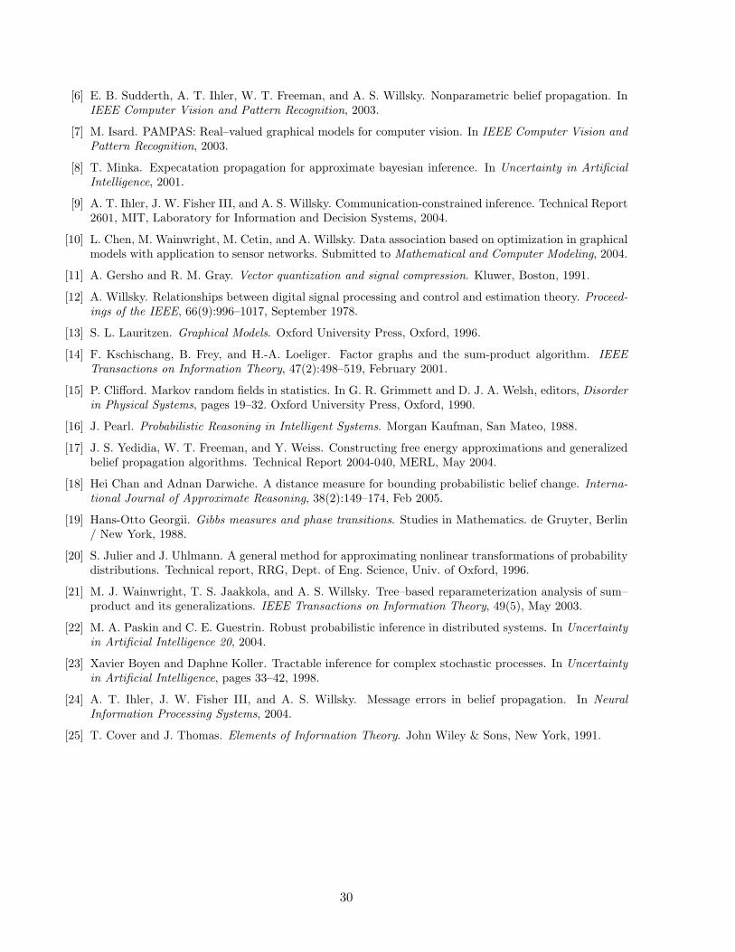
[6] E. B. Sudderth, A. T. Ihler, W. T. Freeman, and A. S. Willsky. Nonparametric belief propagation. InIEEE Computer Vision and Pattern Recognition, 2003.

[7] M. Isard. PAMPAS: Real–valued graphical models for computer vision. In IEEE Computer Vision andPattern Recognition, 2003.

[8] T. Minka. Expecatation propagation for approximate bayesian inference. In Uncertainty in ArtificialIntelligence, 2001.

[9] A. T. Ihler, J. W. Fisher III, and A. S. Willsky. Communication-constrained inference. Technical Report2601, MIT, Laboratory for Information and Decision Systems, 2004.

[10] L. Chen, M. Wainwright, M. Cetin, and A. Willsky. Data association based on optimization in graphicalmodels with application to sensor networks. Submitted to Mathematical and Computer Modeling, 2004.

[11] A. Gersho and R. M. Gray. Vector quantization and signal compression. Kluwer, Boston, 1991.

[12] A. Willsky. Relationships between digital signal processing and control and estimation theory. Proceed-ings of the IEEE, 66(9):996–1017, September 1978.

[13] S. L. Lauritzen. Graphical Models. Oxford University Press, Oxford, 1996.

[14] F. Kschischang, B. Frey, and H.-A. Loeliger. Factor graphs and the sum-product algorithm. IEEETransactions on Information Theory, 47(2):498–519, February 2001.

[15] P. Clifford. Markov random fields in statistics. In G. R. Grimmett and D. J. A. Welsh, editors, Disorderin Physical Systems, pages 19–32. Oxford University Press, Oxford, 1990.

[16] J. Pearl. Probabilistic Reasoning in Intelligent Systems. Morgan Kaufman, San Mateo, 1988.

[17] J. S. Yedidia, W. T. Freeman, and Y. Weiss. Constructing free energy approximations and generalizedbelief propagation algorithms. Technical Report 2004-040, MERL, May 2004.

[18] Hei Chan and Adnan Darwiche. A distance measure for bounding probabilistic belief change. Interna-tional Journal of Approximate Reasoning, 38(2):149–174, Feb 2005.

[19] Hans-Otto Georgii. Gibbs measures and phase transitions. Studies in Mathematics. de Gruyter, Berlin/ New York, 1988.

[20] S. Julier and J. Uhlmann. A general method for approximating nonlinear transformations of probabilitydistributions. Technical report, RRG, Dept. of Eng. Science, Univ. of Oxford, 1996.

[21] M. J. Wainwright, T. S. Jaakkola, and A. S. Willsky. Tree–based reparameterization analysis of sum–product and its generalizations. IEEE Transactions on Information Theory, 49(5), May 2003.

[22] M. A. Paskin and C. E. Guestrin. Robust probabilistic inference in distributed systems. In Uncertaintyin Artificial Intelligence 20, 2004.

[23] Xavier Boyen and Daphne Koller. Tractable inference for complex stochastic processes. In Uncertaintyin Artificial Intelligence, pages 33–42, 1998.

[24] A. T. Ihler, J. W. Fisher III, and A. S. Willsky. Message errors in belief propagation. In NeuralInformation Processing Systems, 2004.

[25] T. Cover and J. Thomas. Elements of Information Theory. John Wiley & Sons, New York, 1991.

30