loom: ery-aware partitioning of online graphs
TRANSCRIPT

Loom:Query-aware Partitioning of Online GraphsHugo Firth
School of Computing [email protected]
Paolo MissierSchool of Computing Science
Jack AistonSchool of Computing Science
ABSTRACTAs with general graph processing systems, partitioning data overa cluster of machines improves the scalability of graph databasemanagement systems. However, these systems will incur addi-tional network cost during the execution of a query workload,due to inter-partition traversals. Workload-agnostic partition-ing algorithms typically minimise the likelihood of any edgecrossing partition boundaries. However, these partitioners aresub-optimal with respect to many workloads, especially queries,which may require more frequent traversal of specific subsets ofinter-partition edges. Furthermore, they are largely unsuited tooperating incrementally on dynamic, growing graphs.
We present a new graph partitioning algorithm, Loom, thatoperates on a stream of graph updates and continuously allocatesthe new vertices and edges to partitions, taking into account aquery workload of graph pattern expressions along with theirrelative frequencies. First we capture the most common patternsof edge traversals which occur when executing queries. We thencompare sub-graphs, which present themselves incrementally inthe graph update stream, against these common patterns. Finallywe attempt to allocate each match to single partitions, reducingthe number of inter-partition edges within frequently traversedsub-graphs and improving average query performance.
Loom is extensively evaluated over several large test graphswith realistic query workloads and various orderings of the graphupdates. We demonstrate that, given a workload, our prototypeproduces partitionings of significantly better quality than existingstreaming graph partitioning algorithms Fennel & LDG.
1 INTRODUCTIONSubgraph pattern matching is a class of operation fundamentalto many “real-time” applications of graph data. For example, insocial networks [9], and network security [3]. Answering a sub-graph pattern matching query usually involves exploring thesubgraphs of a large, labelled graphG then finding those whichmatch a small labelled graph q. Fig.1 shows an example graph Gand a set of query graphs Q which we will refer to throughout.Efficiently partitioning large, growing graphs to optimisefor given workloads of such queries is the primary contribu-tion of this work.
In specialised graph database management systems (GDBMS),pattern matching queries are highly efficient. They usually corre-spond to some index lookup and subsequent traversal of a smallnumber of graph edges, where edge traversal is analogous topointer dereferencing. However, as graphs like social networksmay be both large and continually growing, eventually they sat-urate the memory of a single commodity machine and must bepartitioned and distributed. In such a distributed setting, querieswhich require inter-partition traversals, such as q2 in Fig. 1, in-cur network communication costs and will perform poorly. A
© 2018 Copyright held by the owner/author(s). Published in Proceedings of the 21stInternational Conference on Extending Database Technology (EDBT), March 26-29,2018, ISBN 978-3-89318-078-3 on OpenProceedings.org.Distribution of this paper is permitted under the terms of the Creative Commonslicense CC-by-nc-nd 4.0.
BA1 2 3 4
5 6 7 8
a b c d
b a d c
G Q ( q1:30%, q2:60%, q3:10% )
q3
q1
q2
a
b
b
a
a b c
a b c d
a b
Figure 1: Example graph G with query workload Q
widely recognised approach to addressing these scalability issuesin graph data management is to use one of several k-way balancedgraph partitioners [2, 11, 14, 18, 30–32]. These systems distributevertices, edges and queries evenly across several machines, seek-ing to optimise some global goal, e.g. minimising the number ofedges which connect vertices in different partitions (a.k.a min.edge-cut). In so doing, they improve the performance of a broadrange of possible analyses.
Whilst graphs partitioned for such global measures mostlywork well for global forms of graph analysis (e.g. Pagerank), noone measure is optimal for all types of operation [28]. In particu-lar, the workloads of pattern matching query workloads, commonto GDBMS, are a poor match for these kinds of partitioned graphs,which we call workload agnostic. This is because, intuitively, amin. edge-cut partitioning is equivalent to assuming uniform, orat least constant, likelihood of traversal for each edge through-out query processing. This assumption is unrealistic as a queryworkload may traverse a limited subset of edges and edge types,which is specific to its graph patterns and subject to change.
To appreciate the importance of a workload-sensitive parti-tioning, consider the graph of Fig.1. The partitioning {A,B} isoptimal for the balanced min. edge-cut goal, but may not be op-timal for the query graphs in Q . For example, the query graphq2 matches the subgraphs {(1, 2), (2, 3)} and {(6, 2), (2, 3)} in G.Given a workload which consisted entirely of q2 queries, ev-ery one would require a potentially expensive inter-partitiontraversal (ipt). It is easy to see that the alternative partitioningA′ = {1, 2, 3, 6}, B′ = {4, 5, 7, 8} offers an improvement (0 ipt)given such a workload, whilst being strictly worse w.r.t min.edge-cut.
Mature research of workload-sensitive online database parti-tioning is largely confined to relational DBMS [4, 23, 26]
1.1 ContributionsGiven the above motivation, we present Loom: a partitioner foronline, dynamic graphs which optimises vertex placement toimprove the performance of a given stream of sub-graph patternmatching queries.
The simple goals of Loom are threefold: a) to discover patternsof edge traversals which are common when answering queries
Series ISSN: 2367-2005 337 10.5441/002/edbt.2018.30

from our given workload Q ; b) to efficiently detect instances ofthese patterns in the ongoing stream of graph updates which con-stitutes an online graph; and c) to assign these pattern matcheswholly within an individual partition or across as few partitionsas possible, thereby reducing the number of ipt and increasingthe average performance of any q ∈ Q .
This work extends an earlier “vision” work [7] by the authors,providing the following additional contributions:• A compact 1 trie based encoding of the most frequenttraversal patterns over edges inG. We show how it maybe constructed and updated given an evolving workloadQ .• A method of sub-graph isomorphism checking, extendinga recent probabilistic technique[29]. We show how thismeasure may be efficiently computed and demonstrateboth the low probability of false positives and the impos-sibility of false negatives.• A method for efficiently computing matches for our fre-quent traversal patterns in a graph stream, using our trieencoding and isomorphism method, and then assign thesematching sub-graphs to graph partitions, using heuris-tics to preserve balance. Resulting partitions do not relyupon replication and are therefore agnostic to the complexreplication schemes often used in production systems.
As online graphs are equivalent to graph streams, we presentan extensive evaluation comparing Loom to popular streaminggraph partitioners Fennel [31] and LDG[30]. We partition realand synthetic graph streams of various sizes and with three dis-tinct stream orderings: breadth-first, depth-first and random or-der. Subsequently, we execute query workloads over each graph,counting the number of expensive ipt which occur. Our resultsindicate that Loom achieves a significant improvement over bothsystems, with between 15 and 40% fewer ipt when executing agiven workload.
1.2 Related work
Partitioning graphs into k balanced subgraphs is clearly ofpractical importance to any application with large amounts ofgraph structured data. As a result, despite the fact that the prob-lem is known to be NP-Hard [1], many different solutions havebeen proposed [2, 11, 14, 18, 30–32].We classify these partitioningapproaches into one of three potentially overlapping categories:streaming, non-streaming and workload sensitive. Loom is botha streaming and workload-sensitive partitioner.
Non-streaming graph partitioners [2, 14, 18] typically seek tooptimise an objective function global to the graph, e.g. minimisingthe number of edges which connect vertices in different partitions(min. edge-cut).
A common class of these techniques is known as multi-levelpartitioners [2, 14]. These partitioners work by computing a suc-cession of recursively compressed graphs, tracking exactly howthe graph was compressed at each step, then trivially partition-ing the smallest graph with some existing technique. Using theknowledge of how each compressed graph was produced fromthe previous one, this initial partitioning is then “projected” backonto the original graph, using a local refinement technique (suchas Kernighan-Lin [15]) to improve the partitioning after each step.A well known example of a multilevel partitioner is METIS [14],which is able to produce high quality partitionings for small and1Grows with the size of query graph patterns, which are typically small
medium graphs, but performance suffers significantly in the pres-ence of large graphs [31]. Other mutlilevel techniques [2] sharebroadly similar properties and performance, though they differin the method used to compress the graph being partitioned.
Other types of non-streaming partitioner include Sheep [18]:a graph partitioner which creates an elimination tree from adistributed graph using a map-reduce procedure, then partitionsthe tree and subsequently translates it into a partitioning ofthe original graph. Sheep optimises for another global objectivefunction: minimising the number of different partitions in whicha given vertex v has neighbours (min. communication volume).
These non-streaming graph partitioners suffer from two maindrawbacks. Firstly, due to their computational complexity andhigh memory usage[30], they are only suitable as offline opera-tions, typically performed ahead of analytical workloads. Eventhose partitioners which are distributed to improve scalability,such as Sheep or the parallel implementation ofMETIS (ParMETIS)[14], make strong assumptions about the availability of globalgraph information. As a result they may require periodic re-execution, i.e. given a dynamic graph following a series of graphupdates, which is impractical online [13]. Secondly, as mentioned,partitioners which optimise for such global measures assumeuniform and constant usage of a graph, causing them to “leaveperformance on the table” for many workloads.
Streaming graph partitioners [11, 30, 31] have been proposedto address some of the problems with partitioners outlined above.Firstly, the strict streaming model considers each element of agraph stream as it arrives, efficiently assigning it to a partition.Additionally, streaming partitioners do not perform any refine-ment, i.e. later reassigning graph elements to other partitions,nor do they perform any sort of global introspection, such asspectral analysis. As a result, the memory usage of streamingpartitioners is both low and independent of the size of the graphbeing partitioned, allowing streaming partitioners to scale to tovery large graphs (e.g. billions of edges). Secondly, streamingpartitioners may trivially be applied to continuously growinggraphs, where each new edge or update is an element in thestream.
Streaming partitioners, such as Fennel [31] and LDG [30],make partition assignment decisions on the basis of inexpensiveheuristics which consider the local neighbourhood of each newelement at the time it arrives. For instance, LDG assigns verticesto the partitions where they have the most neighbours, but pe-nalises that number of neighbours for each partition by how fullit is, maintaining balance. By using the local neighbourhood of agraph element e at the time e is added, such heuristics renderthemselves sensitive to the ordering of a graph stream. For ex-ample, a graph which is streamed in the order of a breadth-firsttraversal of its edges will produce a better quality partitioningthan a graph which is streamed in random order, which has beenshown to be pseudo adversarial[31].
In general, streaming algorithms produce partitionings oflower quality than their non-streaming counterparts but withmuch improved performance. However, some systems, such asthe graph partitioner Leopard [11], attempt to strike a balancebetween the two. Leopard relies upon a streaming algorithm (Fen-nel) for the initial placement of vertices but drops the “one-pass”requirement and repeatedly considers vertices for reassignment;improving quality over time for dynamic graphs, but at the costof some scalability. Note that these Streaming partitioners, liketheir non-streaming counterparts, are workload agnostic and soshare those disadvantages.
338

Workload sensitive partitioners [4, 23, 24, 26, 28, 32] attemptto optimise the placement of data to suit a particular workload.Such systems may be streaming or non-streaming, but are dis-cussed separately here because they pertain most closely to thework we do with Loom.
Some partitioners, such as LogGP [32] and CatchW [28], arefocused on improving graph analytical workloads designed forthe bulk synchronous parallel (BSP) model of computation2. In theBSP model a graph processing job is performed in a number ofsupersteps, synchronised between partitions. CatchW examinesseveral common categories of graph analytical workload andproposes techniques for predicting the set of edges likely to betraversed in the next superstep, given the category of workloadand edges traversed in the previous one. CatchW then movesa small number of these predicted edges between supersteps,minimising inter-partition communication. LogGP uses a similarlog of activity from previous supersteps to construct a hyper-graph where vertices which are frequently accessed together areconnected. LogGP then partitions this hypergraph to suggestplacement of vertices, reducing the analytical job’s executiontime in future.
In the domain of RDF stores, Peng et al. [24] use frequentsub-graph mining ahead of time to select a set of patterns com-mon to a provided SPARQL query workload. They then proposepartitioning strategies which ensure that any data matching oneof these frequent patterns is allocated wholly within a singlepartition, thus reducing average query response time at the costof having to replicate (potentially many) sub-graphs which formpart of multiple frequent patterns. Harbi et al. [10] also detectpatterns common to workloads of SPARQL queries; their system,called AdPart, redistributes data between partitions over timesuch that more queries may be executed without ipt . However,like Peng et al’s work, AdPart makes significant use of replication.Additionally, AdPart’s re-partitioning approach relies upon aninitial input generated by a naive Hash partitioner. Thus, it couldpotentially be used in conjunction with a streaming system likeLoom: a workload-aware initial partitioning reducing the amountof data redistribution required later.
For RDBMS, systems such as Schism [4] and SWORD [26]capture query workload samples ahead of time, modelling themas hypergraphs where edges correspond to sets of records whichare involved in the same transaction. These graphs are thenpartitioned using existing non-streaming techniques (METIS)to achieve a min. edge-cut. When mapped back to the originaldatabase, this partitioning represents an arrangement of recordswhich causes a minimal number of transactions in the capturedworkload to be distributed. Other systems, such as Horticulture[23], rely upon a function to estimate the cost of executing asample workload over a database and subsequently explore alarge space of possible candidate partitionings. In addition to ahigh upfront cost [4, 23], these techniques focus on the relationaldata model, and so make simplifying assupmtions, such as ignor-ing queries which traverse > 1-2 edges [26] (i.e. which performnested joins). Larger traversals are common to sub-graph patternmatching queries, therefore its unclear how these techniqueswould perform given such a workload.
Overall, the works reviewed above either focus on differenttypes of workload than we do with Loom (namely offline an-alytical or relational queries), or they make extensive use of
2e.g. Pagerank executed using the Apache Giraph framework: http://bit.ly/2eNVCnv.
replication. Loom does not use any form of replication, both toavoid potentially significant storage overheads [25] and to re-main interoperable with the sophisticated replication schemesused in production systems.
1.3 DefinitionsHere we review and define important concepts used throughoutthe rest of the paper.
A labelled graph G = (V ,E,LV , fl ) is of the form: a set ofverticesV = {v1,v2, ...,vn }, a set of pairwise relationships callededges e = (vi ,vj ) ∈ E and a set of vertex labels LV . The functionfl : V → LV is a surjectivemapping of vertices to labels. Note thatthroughout this work, for simplicity, we consider only undirectedgraphs. However, all techniques subsequently presented may beextended to directed graphs, which we highlight inline. We viewan online graph simply as a (possibly infinite) sequence of edgeswhich are being added to a graphG , over time. We consider fixedwidth sliding windows over such a graph, i.e. a sliding windowof time t is equivalent to the t most recently added edges. Notethat an online may be viewed as a graph stream and we use thetwo terms interchangeably.
A pattern matching query is defined in terms of sub-graphisomorphism. Given a pattern graph q = (Vq ,Eq ), a query shouldreturn R: a set of sub-graphs of G. For each returned sub-graphRi = (VRi ,ERi ) there should exist a bijective function f suchthat: a) for every vertex v ∈ VRi , there exists a correspondingvertex f (v ) ∈ Vq ; b) for every edge (v1,v2) ∈ ERi , there exists acorresponding edge ( f (v1), f (v2)) ∈ Eq ; and c) for every vertexv ∈ Ri , the labels match those of the corresponding verticesin q, l (v ) = l ( f (v )). A query workload is simply a multiset ofthese queries Q = {(q1,n1) . . . (qh ,nh )}, where ni is the relativefrequency of qi in Q .
A query motif is a graph which occurs, with a frequencyof more than some user defined threshold T , as a sub-graph ofquery graphs from a workload Q .
A vertex centric graph partitioning is defined as a disjointfamily of sets of vertices Pk (G ) = {V1,V2, . . . ,Vk }. Each set Vi ,together with its edges Ei (where ei ∈ Ei , ei = (vi ,vj ), and{vi ,vj } ⊆ Vi ), is referred to as a partition Si . A partition forms aproper sub-graph ofG such that Si = (Vi ,Ei ),Vi ⊆ V and Ei ⊆ E.We define the quality of a graph partitioning relative to a givenworkloadQ . Specifically, the number of inter-partition traversals(ipt ) which occurwhile executingQ over Pk (G ).Whilst min. edge-cut is the standard scale free measure of partition quality [14], itis intuitively a proxy for ipt and, as we have argued (Sec. 1), notalways an effective one.
1.4 OverviewOnce again, Loom continuously partitions an online graph Ginto k parts, optimising for a given workload Q . The resultingpartitioning Pk (G,Q ) reduces the probability of expensive ipt ,when executing a random q ∈ Q , using the following techniques.
Firstly, we employ a trie-like datastructure to index all of thepossible sub-graphs of query graphs q ∈ Q , then identify thosesub-graphs which are motifs, i.e. occur most frequently (Sec. 2).Secondly, we buffer a sliding window overG , then use an efficientgraph stream pattern matching procedure to check whether eachnew edge added to G creates a sub-graph which matches one ofour motifs (Sec. 3). Finally, we employ a combination of novel andexisting partitioning heuristics to assign each motif matching
339

a b
c d
b c
b a b
a b c
a b a
b c d
a b a
a b c
b a b
a b c
b
c
a
a b c
a
ab
a
a b c
a
b
b
d
a b c
a
d
b
d
Motif
Low support node
Figure 2: TPSTry++ for Q in fig. 1
sub-graph which leaves the sliding window entirely within anindividual partition, thereby reducing ipt for Q (Sec. 4).
2 IDENTIFYING MOTIFSWe now describe the first of the three steps mentioned above,namely the encoding of all query graphs found in our patternmatching query workload Q . For this, we use a trie-like datas-tructure which we have called the Traversal Pattern SummaryTrie (TPSTry++). In a TPSTry++, every node represents a graph,while every parent node represents a sub-graph which is com-mon to the graphs represented by its children. As an illustration,the complete TPSTry++ for the workload Q in Fig. 1 is shown inFig. 2.
This structure not only encodes all sub-graphs found in eachq ∈ Q , it also associates a support value p with each of its nodes,to keep track of the relative frequency of occurrences of eachsub-graph in our query graphs.
Given a threshold T for the frequency of occurrences, a motifis a sub-graph that occurs at least T times in Q . As an example,for T = 40%, Q’s motifs are the shaded nodes in Fig. 2.
Intuitively, a sub-graph of G which is frequently traversed bya query workload should be assigned to a single partition. Wecan idenfity these sub-graphs as they form within the streamof graph updates, by matching them against the motifs in theTPSTry++. Details of the motif matching process are provided inSec.3. In the rest of this section we explain how a TPSTry++ isconstructed, given a workload Q .
A TPSTry++ extends a simpler structure, called TPSTry, whichwe have recently proposed in a similar setting [8]. It employsfrequent sub-graph mining[12] to compactly encode general la-belled graphs. The resulting structure is a Directed Acyclic Graph(DAG), to reflect the multiple ways in which a particular querypattern may extend shorter patterns. For example in Fig. 2 thegraph in node a-b-a-b can be produced in two ways, by adding asingle a-b edge to either of the sub-graphs b-a-b, and a-b-a. Incontrast, a TPSTry is a tree that encodes the space of possibletraversal paths through a graph as a conventional trie of strings,where a path is a string of vertex labels, and possible paths aredescribed by a stream of regular path queries [20].
Note that the trie is a relatively compact structure, as it growswith |LV |t , where t is the number of edges in the largest querygraph inQ and LV is typically small. Also note that the TPSTry++is similar to, though more general than, Ribiero et al’s G-Trie [27]and Choudhury et al’s SJ-Tree [3], which use trees (not DAGs) toencode unlabelled graphs and labelled paths respectively.
2.1 Sub-graph signaturesWe build the trie for Q by progressively building and mergingsmaller tries for each q ∈ Q , as shown in Fig. 3. This process relies
a
b
b
c
a
b
c
ab
ab
ab
ab
ba
b
ab
a
ab ab
ab
ab
ab
b
a
b
a
b
a
ab
bc
abc
q1
q2
Figure 3: Combining tries for query graphs q1, q2
on detecting graph isomorphisms, as any two trie nodes fromdifferent queries that contain identical graphs should be merged.Failing to detect isomorphism would result, for instance, in twoseparate trie nodes being created for the simple graphs a-b-c andc-b-a, rather than a single node with a support of 2, as intended.One way of detecting isomorphism, often employed in frequentsub-graph mining, involves computing the lexicographical canon-ical form for each graph [19], whereby two graphs are isomorphicif and only if they have the same canonical representation.
Computing a graph’s canonical form provides strong guaran-tees, but can be expensive[27]. Instead, we propose a probabilistic,but computationally more efficient approach based on numbertheoretic signatures, which extends recent work by Song et al. [29].In this approach we compute the signature of a graph as a large,pseudo-unique integer hash that encodes key information suchas its vertices, labels, and nodes degree. Graphs with matchingsignatures are likely to be isomorphic to one another, but thereis a small probability of collision, i.e., of having two differentgraphs with the same signature.
Given a query graph Gq = {Vq ,Eq } we compute its signatureas follows. Initially we assign a random value r (l ) = [1,p), be-tween 1 and some user specified prime p, to each possible labell ∈ LVi from our data graph G; recall that the function fl mapsvertices in G to these labels. We then perform three steps:
(1) Calculate a factor for each edge e = (vi ,vj ) ∈ Eq , accord-ing to the formula:
edдeFac (e ) = (r ( fl (vi )) − r ( fl (vj )))mod p
(2) Calculate the factors that encode the degree of each vertex.If a vertex v has a degree n, its degree factor is defined as:
deдFac (v ) = ((r ( fl (v )) + 1)mod p)·
((r ( fl (v )) + 2)mod p) · . . . · ((r ( fl (v )) + n)mod p)
(3) Finally, we compute the signature of Gq = (Vq ,Eq ) as:
(∏e ∈Ei
edдeFac (e )) · (∏v ∈Vi
deдFac (v ))
Note that for the factors of directed edges, the random value forthe target vertex’s label is subtracted from the random value forthe source vertex’s label (i.e.vj is the target vertex). For undirectededges the ordering of subtraction does not matter, provided it isconsistent (e.g. lexicographical).
To illustrate this signature calculation process, consider queryq1 from Fig. 1. Given a p of 11 and random values r (a) = 3,r (b) = 10 we first calculate the edge factor for an a-b edge:edдeFac ((a,b)) = (3 − 10)mod 11 = 7. As q1 consists of four a-bedges, its total edge factor is 74 = 2401. Then we calculate the
340

degree factors 3, starting with a b labelled vertex with degree 2:deдFac (b) = ((10+1)mod 11) · ((10+2)mod 11) = 11, followed byan a labelled vertex also with degree 2: deдFac (a) = 20. As thereare two of each vertex, with the same degree, the total degreefactor is 112 · 202 = 48400. The signature of q1 = 2401 · 48400 =116208400.
This approach is appealing for two reasons. Firstly, since thefactors in the signature may be multiplied in any order, a signa-ture forG can be calculated incrementally if the signature of anyof its sub-graphsGi is known, as this is the combined factor dueto the additional edges and degree inG \Gi . Secondly, the choiceof p determines a trade-off between the probability of collisionsand the performance of computing signatures. Specifically, notethat signatures can be very large numbers (thousands of bits)even for small graphs, rendering operations such as remaindercostly and slow. A small choice of p reduces signature size, be-cause all the factors are mapped to a finite field [17] (factor modp) between 1 and p, but it increases the likelihood of collision, i.e.,the probability of two unrelated factors being equal. We discusshow to improve the performance and accuracy of signatures inSection 2.3.
2.2 Constructing the TPSTry++
Algorithm 1 Recursively add a query graph Gq to a TPSTry++
1: f actors (e,д) ← degree/edge factors to multiply a graph д’ssignature when adding edge e
2: support (д) ← map of TPSTry++ nodes (graphs) to p-values3: tpstry ← TPSTry++ for workload Q4: parent ← TPSTry++ node, initially root (an empty graph)5: Gq ← query graph defined by a query q6: д ← some sub-graph of Gq
7: for e in edges from Gq do8: д ← new empty graph9: corecurse(parent , e, tpstry,д)10: siд ← f actor (e,д) · parent .siдnature11: if tpstry.siдnatures contains siд then12: n ← node from tpstry with signature siд13: support (n) ← support (n) + 114: else15: n ← new node with graph д + e and signature siд16: support (n) ← 117: tpstry ← tpstry + n18: if not parent .children contains n then19: parent .children ← parent .children + n20: newEdдes ← edges incident to д + e and not in д + e21: for e ′ in newEdдes22: corecurse(n, e ′, tpstry,д + e )23: return tpstry
Our approach to constructing the TPSTry++ is to incremen-tally compute signatures for sub-graphs of each query graph qin a trie, merging trie nodes with equal signatures to produce aDAGwhich encodes the sub-graphs of all q ∈ Q . Alg. 1 formalisesthis approach.
Essentially, we recursively “rebuild” the graphGq | Eq | times,starting from each edge e ∈ Eq in turn. For an edge e we calculateits edge and degree factors, initially assuming a degree of 1 for3Note we don’t consider 0 a valid factor, and replace it with p (e.g. 11mod 11 = 11)
each vertex. If the resulting signature is not associated with achild of the TPSTry++’s root, then we add a node n representinge . Subsequently, we “add” those edges e ′ which are incident toe ∈ Gq , calculating the additional edge and degree factors, andadd corresponding trie nodes as children of n. Then we recurseon the edges incident e + e ′.
Consider again our earlier example of the query graph q1:as it arrives in the workload stream Q , we break it down to itsconstituent edges {a-b, a-b, a-b, a-b}. Choosing an edge at randomwe calculate its combined factor. We know that the edge factorof an a-b edge is 7. When considering this single edge, both aand b vertices have a degree of 1, therefore the signature for a-bis 7 · ((3 + 1) mod 11) · ((10 + 1) mod 11) = 308. Subsquently,we do the same for all other edges and, finding that they havethe same signature, leave the trie unmodified. Next, for eachedge, we add each incident edge from q1 and compute the newcombined signature. Assume we add another a-b edge adjacentto b to produce the sub-graph a-b-a. This produces three newfactors: the new edge factor 7, the new a vertex degree factor((3 + 1)mod 11) and an additional degree factor for the existingb vertex ((10 + 2)mod 11). The combined signature for a-b-a istherefore 308 · 7 · 4 · 1 = 8624; if a node with this signature doesnot exist in the trie as a child of the a-b node, we add it. Thiscontinues recursively, considering larger sub-graphs of q1 untilthere are no edges left in q1 which are not in the sub-graph, atwhich point, q1 has been added to the TPSTry++.
2.3 Avoiding signature collisionsAs mentioned, number theoretic signatures are a probabilisticmethod of ismorphism checking, prone to collisions. There areseveral scenarios in which two non-isomorphic graphs may havethe same signature: a) two factors representing different graphfeatures, such as different edges or vertex degrees, are equal; b)two distinct sets of factors have the same product; and c) twodifferent graphs have identical sets of edges, vertices and vertexdegrees.
The original approach to graph isomorphic checking [29]makes use of an expensive authoritative patternmatchingmethodto verify identified matches. Given a query graph, it calculatesits signature in advance, then incrementally computes signaturesfor sub-graphs which form within a window over a graph stream.If a sub-graph’s signature is ever divisible by that of the querygraph, then that sub-graph should contain a query match.
There are some key differences in howwe compute and use sig-natures with Loom, which allow us to rely solely upon signaturesas an efficient means for mining and matching motifs. Firstly,remember our overall aim is to heuristically lower the probabilitythat sub-graphs in a graphG which match our discovered motifsstraddle a partition boundary. As a result we can tolerate somesmall probability of false positive results, whilst the manner inwhich signatures are executed (Sec. 2.1) precludes false negatives;i.e. two graphs which are isomorphic are guaranteed to have thesame signature. Secondly, we can exploit the structure of theTPSTry++ to avoid ever explicitly computing graph signatures.From Fig. 2 and Alg. 1, we can see that all possible sub-graphsof a query graph Gq will exist in the TPSTry++ by construction.We calculate the edge and degree factors which would multiplythe signature of a sub-graph with the addition of each edge, thenassociate these factors to the relevant trie branches. This allowsus to represent signatures as sets of their constituent factors,
341
0 50 100 150 200 250 300
0.0
0.4
0.8
Probability of acceptance tolerance 5%
P
prob
abilit
y
# of factors243648
0 50 100 150 200 250 300
0.0
0.4
0.8
Probability of acceptance tolerance 10%
P
prob
abilit
y
# of factors243648
0 50 100 150 200 250 300
0.0
0.4
0.8
Probability of acceptance tolerance 20%
P
prob
abilit
y
# of factors243648
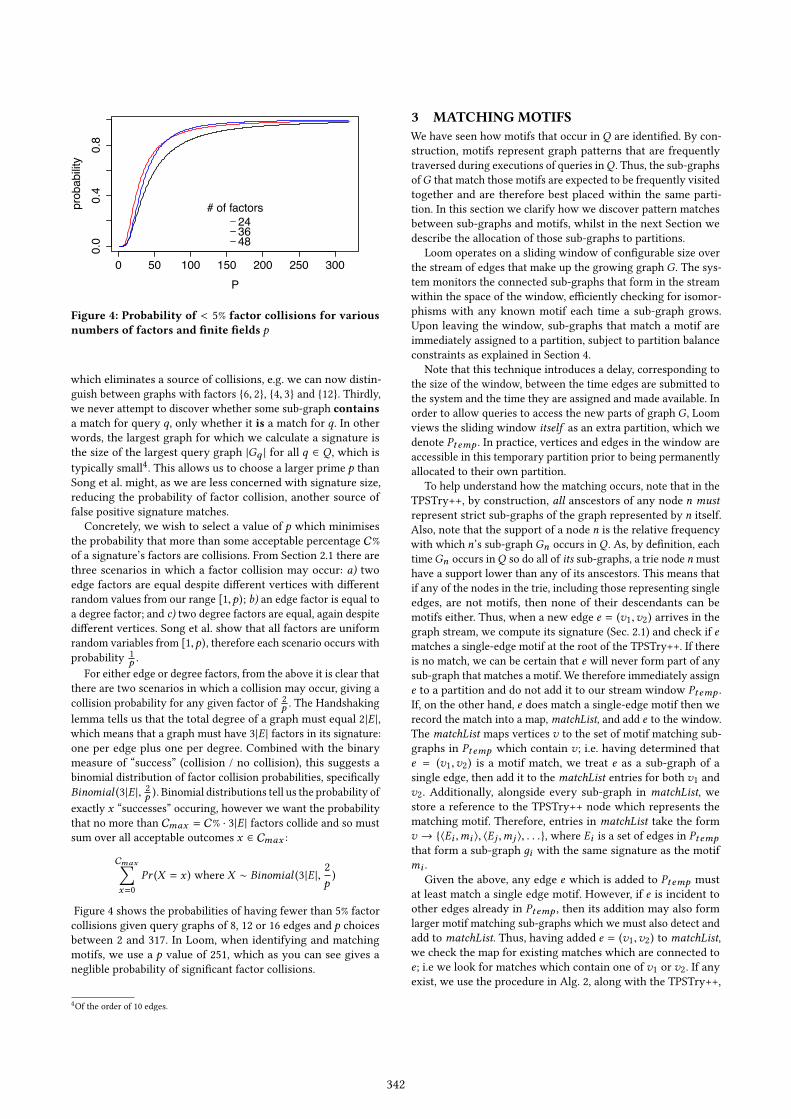
Figure 4: Probability of < 5% factor collisions for variousnumbers of factors and finite fields p
which eliminates a source of collisions, e.g. we can now distin-guish between graphs with factors {6, 2}, {4, 3} and {12}. Thirdly,we never attempt to discover whether some sub-graph containsa match for query q, only whether it is a match for q. In otherwords, the largest graph for which we calculate a signature isthe size of the largest query graph |Gq | for all q ∈ Q , which istypically small4. This allows us to choose a larger prime p thanSong et al. might, as we are less concerned with signature size,reducing the probability of factor collision, another source offalse positive signature matches.
Concretely, we wish to select a value of p which minimisesthe probability that more than some acceptable percentage C%of a signature’s factors are collisions. From Section 2.1 there arethree scenarios in which a factor collision may occur: a) twoedge factors are equal despite different vertices with differentrandom values from our range [1,p); b) an edge factor is equal toa degree factor; and c) two degree factors are equal, again despitedifferent vertices. Song et al. show that all factors are uniformrandom variables from [1,p), therefore each scenario occurs withprobability 1
p .For either edge or degree factors, from the above it is clear that
there are two scenarios in which a collision may occur, giving acollision probability for any given factor of 2
p . The Handshakinglemma tells us that the total degree of a graph must equal 2|E |,which means that a graph must have 3|E | factors in its signature:one per edge plus one per degree. Combined with the binarymeasure of “success” (collision / no collision), this suggests abinomial distribution of factor collision probabilities, specificallyBinomial (3|E |, 2p ). Binomial distributions tell us the probability ofexactly x “successes” occuring, however we want the probabilitythat no more than Cmax = C% · 3|E | factors collide and so mustsum over all acceptable outcomes x ∈ Cmax :
Cmax∑x=0
Pr (X = x ) where X ∼ Binomial (3|E |, 2p)
Figure 4 shows the probabilities of having fewer than 5% factorcollisions given query graphs of 8, 12 or 16 edges and p choicesbetween 2 and 317. In Loom, when identifying and matchingmotifs, we use a p value of 251, which as you can see gives aneglible probability of significant factor collisions.
4Of the order of 10 edges.
3 MATCHING MOTIFSWe have seen how motifs that occur in Q are identified. By con-struction, motifs represent graph patterns that are frequentlytraversed during executions of queries inQ . Thus, the sub-graphsofG that match those motifs are expected to be frequently visitedtogether and are therefore best placed within the same parti-tion. In this section we clarify how we discover pattern matchesbetween sub-graphs and motifs, whilst in the next Section wedescribe the allocation of those sub-graphs to partitions.
Loom operates on a sliding window of configurable size overthe stream of edges that make up the growing graph G. The sys-tem monitors the connected sub-graphs that form in the streamwithin the space of the window, efficiently checking for isomor-phisms with any known motif each time a sub-graph grows.Upon leaving the window, sub-graphs that match a motif areimmediately assigned to a partition, subject to partition balanceconstraints as explained in Section 4.
Note that this technique introduces a delay, corresponding tothe size of the window, between the time edges are submitted tothe system and the time they are assigned and made available. Inorder to allow queries to access the new parts of graph G, Loomviews the sliding window itself as an extra partition, which wedenote Ptemp . In practice, vertices and edges in the window areaccessible in this temporary partition prior to being permanentlyallocated to their own partition.
To help understand how the matching occurs, note that in theTPSTry++, by construction, all anscestors of any node n mustrepresent strict sub-graphs of the graph represented by n itself.Also, note that the support of a node n is the relative frequencywith which n’s sub-graphGn occurs in Q . As, by definition, eachtimeGn occurs inQ so do all of its sub-graphs, a trie node n musthave a support lower than any of its anscestors. This means thatif any of the nodes in the trie, including those representing singleedges, are not motifs, then none of their descendants can bemotifs either. Thus, when a new edge e = (v1,v2) arrives in thegraph stream, we compute its signature (Sec. 2.1) and check if ematches a single-edge motif at the root of the TPSTry++. If thereis no match, we can be certain that e will never form part of anysub-graph that matches a motif. We therefore immediately assigne to a partition and do not add it to our stream window Ptemp .If, on the other hand, e does match a single-edge motif then werecord the match into a map, matchList, and add e to the window.The matchList maps vertices v to the set of motif matching sub-graphs in Ptemp which contain v; i.e. having determined thate = (v1,v2) is a motif match, we treat e as a sub-graph of asingle edge, then add it to the matchList entries for both v1 andv2. Additionally, alongside every sub-graph in matchList, westore a reference to the TPSTry++ node which represents thematching motif. Therefore, entries in matchList take the formv → {⟨Ei ,mi ⟩, ⟨Ej ,mj ⟩, . . .}, where Ei is a set of edges in Ptempthat form a sub-graph дi with the same signature as the motifmi .
Given the above, any edge e which is added to Ptemp mustat least match a single edge motif. However, if e is incident toother edges already in Ptemp , then its addition may also formlarger motif matching sub-graphs which we must also detect andadd to matchList. Thus, having added e = (v1,v2) to matchList,we check the map for existing matches which are connected toe; i.e we look for matches which contain one of v1 or v2. If anyexist, we use the procedure in Alg. 2, along with the TPSTry++,
342

1
2
3
4
5
{<e1, m1>, <{e1,e4}, m3>, … }
{<e1, m1>, <e4, m2> , <{e1,e4}, m3>, … }
{<e2, m1>, … }
{<e4, m2>, <e3, m2>, <{e1,e4}, m3>, … }
t
1a
2b
3a
4b
5c
e1 e2
e3e4
e5
a b
b c
b a b
a b c
a b a
a b a b
m5
m2
m1
m4
m3
m6
{<e3, m2>, … }
Figure 5: t-length window over G (left), Motifs from TPSTry++ (center) and motifmatchList for window (right)
Algorithm 2Mine motif matches from each new edge e ∈ G1: f actors (e,д) ← degree/edge factors to multiply a graph д’s
signature when adding edge e2: tpstry ← filtered TPSTry++ of motifs for workload Q
3: for each new edge e (v1,v2) do4: matches ←matchList (v1) ∪matchList (v2)5: for each sub-graphm inmatches do6: n ← the tpstry node form7: if n has child c w. f actor = f actors (e,m) then8: add ⟨m + e, c⟩ tomatchList for v1&v2 //Match found!9: ms1 ←matchList (v1)10: ms2 ←matchList (v2)11: for all possible pairs (m1,m2) from (ms1,ms2) do12: n1 ← the tpstry node form113: recurse(tpstry,m2,m1,n1)14: for each edge e2 inm2 do15: if n1 has child c1 w. f actor = f actors (e2,m1) then16: recurse(tpstry,m2 − e2,m1 + e2, c1)17: if m2 is empty then //Match found!18: add ⟨m1 +m2,n1⟩ tomatchList for v1&v2
to determine whether the addition of edge e to these sub-graphscreates another motif match.
Essentially, for each sub-graph дi from matchList to whiche is connected, we calculate the set of edge and degree factorsf ac (e,дi ) which would multiply the signature of дi upon theaddition e , as in Sec. 2. Recall, also from Sec. 2, that a TPSTry++node contains a signature for the graph it represents, and thatthese signatures are stored as sets of factors, rather than theirlarge integer products. As each sub-graph in matchList is pairedwith its associated motif n from the trie, we can efficiently checkif n has a child c where a) c is a motif; and b) the differencebetween n’s factor set and c’s factor set corresponds to factors forthe addition of e toдi , i.e., f ac (e,дi ) = c .siдnatures\n.siдnatures .If such a child exists in the trie then adding e to a graph whichmatches motif n (дi ) will likely create a graph which matchesmotif c: the addition of e to Ptemp has formed the new motifmatching sub-graph дi + e .
We also detect if the joining of two existing multi edge motifmatches (⟨E1,m1⟩, ⟨E2,m2⟩) forms yet another motif match, inroughly the same manner. First we consider each edge from thesmaller motif match (e.g. e ∈ E2 from ⟨E2,m2⟩), checking if theaddition of any of these edges to E15 constitutes yet anothermatch; if it does then we add the edge to E1 and recursivelyrepeat the process until E2 is empty. If this process does exhaustE2 then E1 ∪ E2 constitute a motif matching sub-graph. Oncethis process is complete, matchList will contain entries for all of
5Treating E1 as a sub-graph.
the motif matching sub-graphs currently in Ptemp . Note that asmore edges are added to Ptemp , matchList may contain multipleentries for a given vertex where one match is a sub-graph ofanother, i.e. new motif matches don’t replace existing ones.
As an example of the motif matching process, consider theportion of a graph stream (left), motifs (center) and matchList(right) depicted in Fig. 5. Our window over the graph streamGis initially empty, with the depicted edges being added in labelorder (i.e. e1, e2, . . .). As the edge e1 is added, we first computeits signature and verify whether e1 matches a single-edge motifin the TPSTry++. We can see that, as an a-b labelled edge, thesignature for e1 must match that of motifm1, therefore we adde1 to Ptemp , and add the entry ⟨e1,m1⟩ to matchList for both e1’svertices 1,2. As e1 is not yet connected to any other edges inPtemp , we do not need to check for the formation of additionalmotif matches. Subsequently, we perform the exact same processfor edge e2. When e3 is added, again we verify that, as a b-cedge, e3 is a match for the single-edge motifm3 and so updatePtemp and matchList accordingly. However, e3 is connected toexisting motif matching sub-graphs in Ptemp therefore the unionof matchList entries for e3’s vertices 4,5 (line 4 Alg. 2) returns{⟨e2,m1⟩}. As a result, we calculate the factors to multiply e2’ssignature by, when adding e3. Remember that when computingsignatures, each edge has a factor, as well as each degree. Thus,when adding e3 to e2 our new factors are an edge factor for ab-c labelled edge, a first degree factor for the vertex labelled c (5)and a second degree factor for the vertex labelled b6 (4) (Sec. 2.1).Subsquently we must check whether the motif for e2,m1, has anychild nodes with additional factors consistent with the additionof a b-c edge, which it does:m3. This means we have found anew sub-graph in Ptemp which matches the motifm3, and mustadd ⟨{e2, e3},m3⟩ to the matchList entries for vertices 3, 4 and 5.Similarly, the addition of b-c labelled edge e4 to our graph streamproduces the new motif matches ⟨e4,m2⟩ and ⟨{e1, e4},m3⟩, ascan be seen in our example matchList.
Finally, the addition of our last edge, e5, creates several newmotif matches (e.g. ⟨{e1, e5},m4⟩, ⟨{e2, e5},m5⟩ etc. . . ). In particu-lar, notice that the addition of e5 creates a match for the motifm6,combining the new motif match ⟨{e1, e5},m4⟩ with an existingone ⟨e2,m1⟩. To understand how we discover these slightly morecomplex motif matches, consider Alg. 2 from line 11 onwards.First we retrieve the updated matchList entries for vertices 2 and3, including the new motif matches gained by simply adding thesingle edge e5 to connected existing motif matches, as above.Next we iterate through all possible pairs of motif matches forboth vertices. Given the pair of matches (⟨{e1, e5},m4⟩, ⟨e2,m1⟩),we discover that the addition of any edge from the smaller match(i.e. e2) to the larger produces factors which correspond to a childofm4 in the TPSTry++:m6. As e2 is the only edge in the smaller
6As, with the addition of e3 , vertex 4 has degree 2.
343

match, we simply add the match ⟨{e1, e2, e5},m6⟩ to thematchListentries for 1, 2, 3 and 4. In the general case however, we wouldnot add this new match but instead recursively “grow” it withnew edges from the smaller match, updating matchList only ifall edges from the smaller match have been successfully added.
4 ALLOCATING MOTIFSFollowing graph stream pattern matching, we are left with acollection of sub-graphs, consisting solely of the most recent tedges in G, which match motifs from Q . As new edges arrive inthe graph stream, our window Ptemp grows to size t and then“slides”, i.e. each new edge added to a full window causes theoldest (t + 1th ) edge e to be dropped. Our strategy with Loomis to then assign this old edge e to a permanent partition, alongwith the other edges in the window which form motif matchingsub-graphs with e . The sole exception to this is when an edgearrives that may not form part of any motif match and is assignedto a partition immediately (Sec. 3). This exception does not pose aproblem however, because Loom behaves as if the edge was neveradded to the window and therefore does not cause displacementof older edges.
Recall again that with Loom we are attempting to assignmotif matching sub-graphs wholly within individual partitionswith the aim of reducing ipt when executing our query work-load Q . One naive approach to achieving this goal is as fol-lows: When assigning an edge e = (v1,v2), retrieve the mo-tif matches associated with v1 and v2 from Ptemp using ourmatchList map, then select the subsetMe that contains e , whereMe = {⟨E1,m1⟩, . . . ⟨En ,mn⟩}, e ∈ Ei and Ei is a match formi .Finally, treating these matches as a single sub-graph, assign themto the partition which they share the most incident edges. Thisapproach would greedily ensure that no edges belonging to mo-tif matching sub-graphs in G ever cross a partition boundary.However, it would likely also have the effect of creating highlyunbalanced partition sizes, portentially straining the resources ofa single machine, which prompted partitioning in the first place.
Instead, we rely upon two distinct heuristics for edge assign-ment, both of which are aware of partition balance. Firstly, for thecase of non-motif-matching edges that are assigned immediately,we use the existing Linear Deterministic Greedy (LDG) heuristic[30]. Similar to our naive solution above, LDG seeks to assignedges7 to the partition where they have the most incident edges.However, LDG also favours partitions with higher residual capac-ity when assigning edges in order to maintain a balanced numberof vertices and edges between each. Specifically, LDG defines theresidual capacity r of a partition Si in terms of the number ofvertices currently in Si , given asV (Si ), and a partition capacityconstraintC : r (Si ) = 1− |V (Si ) |
C . When assigning an edge e , LDGcounts the number of e’s incident edges in each partition, givenas N (Si , e ), and weights these counts by Si ’s residual capacity; eis assigned to the partition with the highest weighted count. Thefull formula for LDG’s assignment is:
maxSi ∈Pk (G )
N (Si , e ) · (1 −|V (Si ) |
C)
Secondly, for the general case where edges form part of mo-tif matching sub-graphs, we propose a novel heuristic, equalopportunism. Equal opportunism extends ideas present in LDGbut, when assigning clusters of motif matching sub-graphs to asingle partition as we do in Loom, it has some key advantages.
7LDG may partition either vertex or edge streams.
By construction, given an edge e to be assigned along with itsmotif matches Me = {⟨E1,m1⟩ . . . ⟨En ,mn⟩}, the sub-graphs EiEj inMe have significant overlap (e.g. they all contain e). Thus,individually assigning each motif match to potentially differentpartitions would create many inter-partition edges. Instead, equalopportunism greedily assigns the match cluster to the single par-tition with which it shares the most vertices, weighted by eachpartition’s residual capacity. However, as these vertices and theirnew motif matching edges may not be traversed with equal like-lihood given a workload Q , equal opportunism also prioritisesthe shared vertices which are part of motif matches with highersupport in the TPSTry++.
Formally, given the motif matches Me we compute a scorefor each partition Si and motif match ⟨Ek ,mk ⟩ ∈ Me , which wecall a bid. Let N (Si ,Ek ) = |V (Si ) ∩V (Ek ) | denote the numberof vertices in the edge set Ek (which is itself a graph) that arealready assigned to Si 8. Additionally, let supp (mk ) refer to thesupport of motifmk in the TPSTry++ and recall that C is a ca-pacity constraint defined for each partition. We define the bidfor partition Si and motif match ⟨Ek ,mk ⟩ as:
bid (Si , ⟨Ek ,mk ⟩) = N (Si ,Ek ) · (1 −|V (Si ) |
C) · supp (mk ) (1)
We could simply assign the cluster of motif matching sub-graphs (i.e. E1 ∪ . . . ∪ En ) to the single partition Si with thehighest bid for all motif matches in Me . However, equal op-portunism further improves upon the balance and quality ofpartitionings produced with this new weighted approach, lim-iting its greediness using a rationing function we call l . l (Si ) isa number between 0 and 1 for each partition, the size of whichis inversely correlated with Si ’s size relative to the smallest par-tition Smin = minS ∈Pk (G ) |V (S ) |, i.e. if Si is as small as Sminthen l (Si ) = 1. Equal opportunism sorts motif matches in Mein descending order of support, then uses l (Si ) to control boththe number of matches used to calculate partition Si ’s total bid,and the number of matches assigned to Si should its total bid bethe highest. This strategy helps create a balanced partitioning bya) allowing smaller partitions to compute larger total bids overmore motif matches; and b) preventing the assignment of largeclusters of motif matches to an already large partition. Formallywe calculate l (Si ) as follows:
l (Si ) =|V (Si ) |
Smin· α , α =
1, |V (Si ) | = |V (Smin ) |
0, |V (Si ) | > |V (Smin ) | · b
α , otherwise(2)
where α is a user specified number 0 < α ≤ 1 which controlsthe aggression with which l penalises larger partitions and blimits the maximum imbalance. Throughout this work we usean empirically chosen default of α = 2
3 and set the maximumimbalance to b = 1.1, emulating Fennel [31].
Given definitions (1) and (2), we can now simply state theoutput of equal oppurtinism for the sorted set of motif matchesMe , as:
maxSi ∈Pk (G )
l (Si ) · |Me |∑k=0
bid (Si , ⟨Ek ,mk ⟩) (3)
Note that motif matches in Me which are not bid on by thewinning partition are dropped from thematchList map, as someof their constituent edges (e.g. e , which all matches in Me share)have been assigned to partitions and removed from the slidingwindow Ptemp .8Note that N is a generalisation of LDG’s function N
344

To understand how to the rationing function l improves thequality of equal opportunism’s partitioning, not just its balance,consider the following: Just because an edge e ′ falls within themotif match setMe of our assignee e , does not necessarily implythat placing them within the same partition is optimal. e ′ couldbe a member of many other motif matches in Ptemp besides thoseinMe , perhaps with higher support in the TPSTry++ (i.e. higherlikelihood of being traversed when executing a workload Q). Byordering matches by support and prioritising the assignmentof the smaller, higher support motif matches, we often leavee ′ to be assigned later along with matches to which it is more“important”.
As an example, consider again the graph and TPSTry++ frag-ment in Fig. 5. If assigning the edge e1 to a partition at thetime t + 1, its support ordered set of motif matchesMe1 wouldbe ⟨e1,m1⟩, ⟨{e1, e4},m3⟩, ⟨{e1, e5},m4⟩ and ⟨{e1, e2, e5},m6⟩. As-sume two partitions S1 and S2, where S1 is 33.3% larger thanS2 and vertex 2 already belongs to partition S1, whilst all othervertices in the window are as yet unassigned (i.e. this is the firsttime edges containing them have entered the sliding window).In this scenario, S1 is guaranteed to win all bids, as S2 containsno vertices fromMe1 and therefore N (S2, _) will always equal 0.However, rather than greedily assign all matches to the alreadylarge S1, we calculate the ration l for S1 as 1
1.33 ·11.5 =
12 , given
α = 1.5. In other words, we only assign edges from the first half ofMe1 (⟨e1,m1⟩, ⟨{e1, e4},m3⟩) to S1; edges such as e5 and e2 remainin the window Ptemp . Assume an edge e6 = (4, 6) subsequentlyarrives in the graph stream G , where vertex 6 already belongs topartition S2 and e6 matches the motifm2 (i.e. has labels b-c). If wehad already assigned e5 to partition S1 then this would lead to aninter-partition edge which is more likely to be traversed togetherwith e5 than are other edges in S1, given our workloadQ . Instead,we compute a match in Ptemp between {e5, e6} and the motifm3,and will likely later assign e5 to partition S2. Within reason, thelonger an edge remains in the sliding window, the more of itsneighbourhood information we are likely to have access to, thebetter partitioning decisions we can make for it.
5 EVALUATIONOur evaluation aims to demonstrate that Loom achieves highquality partitionings of several large graphs in a single-pass,streaming manner. Recall that we measure graph partitioningquality using the number of inter-partition traversals when ex-ecuting a realistic workloads of pattern matching queries overeach graph.
Loom consistently produces partitionings of around 20% supe-rior quality when compared to those produced by state of the artalternatives: LDG [30] and Fennel [31] Furthermore, Loom parti-tionings’ quality improvement is robust across different numbersof partitions (i.e. a 2-way or a 32-way partitioning). Finally weshow that, like other streaming partitioners, Loom is sensitiveto the arrival order of a graph stream, but performs well given apseudo-adversarial random ordering.
5.1 Experimental setupFor each of our experiments, we start by streaming a graph fromdisk in one of three predefined orders: Breadth-first: computedby performing a breadth-first search across all the connected com-ponents of a graph;Random: computed by randomly permutingthe existing order of a graph’s elements; and Depth-first: com-puted by performing a depth-first search across the connected
Entity
Activity
Entity Paper
Person Person
PaperPaperAgent
Artist
Label
Area
Area
DBLPProvGen MusicBrainz
Figure 6: Examples of q forMusicBrainz, DBLP & ProvGen
components of a graph. We choose these stream orderings asthey are common to the evaluations of other graph stream parti-tioners [11, 22, 30, 31], including LDG and Fennel.
Subsequently, we produce 4 separate k-way partitionings ofthis ordered graph stream, using each of the following partition-ing approaches for comparison: Hash: a naive partitioner whichassigns vertices and edges to partitions on the basis of a hashfunction. As this is the default partitioner used by many exist-ing partition graph databases9, we use it as a baseline for ourcomparisons. LDG: a simple graph stream partitioner with goodperformance which we extend with our work on Loom. Fennel:a state-of-the-art graph stream partitioner and our primary pointof comparison. As suggested by Tsourakakis et al, we use the Fen-nel parameter value γ = 1.5 throughout our evaluation. Loom:our own partitioner which, unless otherwise stated, we invokewith a window size of 10k edges and a motif support thresholdof 40%.
Finally, when each graph is finished being partitioned, weexecute the appropriate query workload over it and count thenumber of inter-partition traversals (ipt ) which occur.
Note that we avoid implementation dependent measures ofpartitioning quality because, as an isolated prototype, Loom isunlikely to exhibit realistic performance. For instance, lacking adistributed query processing engine, query workloads are exe-cuted over logical partitions during the evaluation. In the absenceof network latency, query response times are meaningless as ameasure of partitioning quality.
All algorithms, data structures, datasets and query workloadsare publicly available10. All our experiments are performed ona commodity machine with a 3.1Ghz Intel i7 CPU and 16GB ofRAM.
5.1.1 Graph datasets. Remember that the workload-agnosticpartitioners which we aim to supersede with Loom are liableto exhibit poor workload performance when queries focus ontraversing a limited subset of edge types (Sec. 1). Intuitively, suchskewed workloads are more likely over heterogeneous graphs,where there exist a larger number of possible edge types forqueries to discern between, e.g. a-a, a-b, a-c . . . vs just a-a. Thus,we have chosen to test the Loom partitioner over five datasetswith a range of different heterogeneities and sizes; three of thesedatasets are synthetic and two are real-world. Table 1 presentsinformation about each of our chosen datasets, including theirsize and how heterogeneous they are (|LV |). We use the DBLP,and LUBM datasets, which are well known. MusicBrainz11 is afreely available database of curated music metadata, with vertex
9The Titan graph database: http://bit.ly/2ejypXV10The Loom repository: http://bit.ly/2eJxQcp11The MusicBrainz database: http://bit.ly/1J0wlNR
345

(a) Random order (b) Breadth-first order (c) Depth-first order
Figure 7: ipt %, vs. Hash, when executing Q over 8-way partitionings of graph streams in multiple orders.
(a) k = 2 (b) k = 8 (c) k = 32
Figure 8: ipt %, vs. Hash, when executing Q over multiple k-way partitionings of breadth-first graph streams.
Dataset ∼ |V | ∼ |E | |LV | Real DescriptionDBLP 1.2M 2.5M 8 Y Publications & citationsProvGen 0.5M 0.9M 3 N Wiki page provenanceMusicBrainz 31M 100M 12 Y Music records metadataLUBM-100 2.6M 11M 15 N University recordsLUBM-4000 131M 534M 15 N University recordsTable 1: Graph datasets, incl. size & heterogeneity
labels such as Artist, Country, Album and Label. ProvGen[6] isa synthetic generator for PROV metadata [21], which recordsdetailed provenance for digital artifacts.
5.1.2 Query workloads. For each dataset we must propose arepresentative query workload to execute so that we may mea-sure partitioning quality in terms of ipt . Remember that a queryworkload consists of a set of distinct query patterns along with afrequency for each (Sec. 1.3). The LUBM dataset provides a set ofquery patterns which we make use of. For every other dataset,however, we define a small set of common-sense queries whichfocus on discovering implicit relationships in the graph, such aspotential collaboration between authors or artists 12. The fulldetails of these query patterns are elided for space10, howeverFig. 6 presents some examples. Note that whilst the TPSTry++may be trivially updated to account for change in the frequenciesof workload queries (Sec. 2), our evaluation of Loom assumesthat said frequencies are fixed and known a priori. Recall that, foronline databases, we argue this is a realistic assumption (Sec. 1).However, more complete tests with changing workloads are animportant area for future work.
12If possible, workloads are drawn from the literature, e.g. common PROVqueries [5]
5.2 Comparison of systemsFigures 7 and 8 present the improvement in partitioning qualityachieved by Loom and each of the comparable systems we desribeabove. Initially, consider the experiment depicted in Fig. 7. Wepartition ordered streams of each of our first 4 graph datasets13into 8-way partitionings, using the approaches described above,then execute each dataset’s query workload over the appropriatepartitioning. The absolute number of inter-partition traversals(ipt ) suffered when querying each dataset varies significantly.Thus, rather than represent these results directly, in Fig. 7 (and 8)we present the results for each approach as relative to the re-sults for Hash; i.e. how many ipt did a partitioning suffer, as apercentage of those suffered by the Hash partitioning of thesame dataset.
As expected, the naive hash partitioner performs poorly: itproduces partitionings which suffer twice as many inter-partitiontraversals, on average, when compared to partitionings producedby the next best system (LDG). Whilst the LDG partitioner doesachieve around a 55% reduction in ipt vs our Hash baseline, itsproduces partitionings of consistently poorer quality than thoseof Fennel and Loom. Although both LDG and Fennel optimisetheir partitionings for the balanced min. edge-cut goal (Sec. 1),Fennel is the more effective heuristic, cutting around 25% feweredges than LDG for small numbers of partitions (including k =8) [31]. Intuitively, the likelihood of any edge being cut is a coarseproxy for the likelihood of a query q ∈ Q traversing a cut edge.This explains the disparity in ipt scores between the two systems.
Of more interest is comparing the quality of partitionings pro-duced by Fennel and Loom. Fig. 7 clearly demonstrates that Loomoffers a significant improvement in partitioning quality over Fen-nel, given a workload Q . Loom’s reduction in ipt relative toFennel’s is present across all datasets and stream orders, however13Excluding LUBM-4000
346

Dataset LDG (ms) Fennel (ms) Loom (ms) Hash (ms)DBLP 91 96 235 28ProvGen 144 146 240 33MusicBrainz 48 52 129 18LUBM-100 47 51 147 22LUBM-4000 45 49 138 16
Table 2: Time to partition 10k edges
it is particularly pronounced over ordered streams of more het-erogeneous graphs; e.g. MusicBrainz in Sub-figure 8b(b), whereLoom’s partitioning suffers from 42% fewer ipt than Fennel’s.This makes sense because, as mentioned, pattern matching work-loads are more likely to exhibit skew over heterogeneous graphs,where query graphs Gq contain a, potentially small, subset ofthe possible vertex labels. Across all the experiments presentedin Fig. 7, the median range of Loom’s ipt reduction relative toFennel’s is 20 − 25%. Additionally, Fig. 8 demonstrates that thisimprovement is consistent for different numbers of partitions. Asthe number of partitions k grows, there is a higher probabilitythat vertices belonging to a motif match are assigned across mul-tiple partitions. This results in an increase of absolute ipt whenexecuting Q over a Loom partitioning. However, increasing kactually increases the probability that any two vertices whichshare an edge are split between partitions, thus reducing the qual-ity of Hash, LDG and Fennel partitionings as well. As a result,the difference in relative ipt is largely consistent between all 4systems.
On the other hand, neither Fig. 7, nor Fig. 8, present the run-time costs of producing a partitioning. Table 2 presents how long(in ms) each partitioner takes to partition 10k edges. Whilst all 3algorithms are capable of partitioning many 10s of thousands ofedges per second, we do find that Loom is slower than LDG andFennel by an average factor of 2-3. This is likely due to the morecomplex map-lookup and pattern-matching logic performed byLoom, or a nascent implementation. The runtime performanceof Loom varies depending on the query workload Q used to gen-erate the TPSTry++ (Sec. 2), therefore the performance figurespresented in Table 2 are averaged across many different Q . Theminimum slowdown factor observed between Loom and Fennelwas 1.5, the maximum 7.1. Note that popular non-streaming par-titioner METIS [14] is around 13 times slower than Fennel forlarge graphs [31].
We contend that this performance difference is unlikely to bean issue in an online setting for two reasons. Firstly, most produc-tion databases do not support more than around 10k transactionsper second (TPS) [16]. Secondly, it is considered exceptional foreven applications such as twitter to experience >30k-40k TPS 14.Meanwhile, the lowest partitioning rate exhibited by Loom inTable 2 is equivalent to ~ 42k edges per second, the highest 72k.
Note that Figures 7 and 8 do not present the relative ipt figuresfor the LUBM-4000 dataset. This is because measuring relative iptinvolves reading a partitioned graph into memory, which is be-yond the constraints of our present experimental setup. However,we include the LUBM-4000 dataset in Table 2 to demonstrate that,as a streaming system, Loom is capable of partitioning large scalegraphs. Also note that none of the figures present partitioningimbalance as this is broadly similar between all approaches and
14Tweets per second in 2013: http://bit.ly/2hQH5JJ
Figure 9: ipt (y-axis) when executing Q over Loom parti-tionings with multiple window sizes t (x-axis)
datasets 15, with LDG varying between 1%−3%, Loom and Fennelbetween 7% and their maximum imbalance of 10% (Sec. 4).
5.3 Effect of stream order and window sizeFig. 7 indicates that Loom is sensitive to the ordering of its givengraph stream. In fact, Sub-figure 7(a) shows Loom achieve asmaller reduction in ipt over Fennel and LDG, than in 7(b) and7(c). Specifically Loom achieves a 42% greater reduction in relativeipt than Fennel given a breadth-first stream of the MusicBrainzgraph, but only a 26% when the stream is ordered randomly,despite Fennel and LDG also being sensitive to stream order-ing [30, 31]. This implies that Loom is particularly sensitive torandom orderings: edges which are close to one another in thegraph may not be close in the graph stream, resulting in Loomdetecting fewer motif matching subgraphs in its stream window.
Intuitively, this sensitivity can be ameliorated by increasingthe size of Loom’s window, as shown in Fig. 9 As Loom’s windowgrows, so does the probability that clusters of motif matchingsubgraphs will occur within it. This allows Loom’s equal oppor-tunism heuristic to make the best possible allocation decisionsfor the subgraph’s constituent vertices. Indeed, the number ofipt suffered by Loom partitionings improves significantly, by asmuch as 47%, as the window size grows from 100 to 10k. However,increasing the window size past 10k clearly has little effect onipt suffered to execute Q if your graph stream is ordered. Theexact impact of increasing Loom’s window size depends uponthe degree distribution of the graph being partitioned. However,to gain an intuition consider the naive case of a graph with a uni-form average vertex degree of 8, along with a TPSTry++ whoselargest motif contains 4 edges. In this case, a breadth-first traver-sal of 84 edges from a vertex a (i.e. window size t ≈ 4k) is highlylikely to include all the motif matches which contain a. Regard-less, Fig. 9 might seem to suggest that Loom should run with thelargest window size possible. However, besides the additionalcomputational cost of detecting more motif matches, rememberthat Loom’s window constitutes a temporary partition (Sec. 3). Ifthere exist many edges between other partitions and Ptemp , thenthis may itself be a source of ipt and poor query performance.
15Except Hash, which is balanced.
347
6 CONCLUSIONS AND FUTUREWORKIn this paper, we have presented Loom: a practical system forproducing k-way partitionings of online, dynamic graphs, whichare optimised for a given workload of pattern matching queriesQ . Our experiments indicate that Loom significantly reduces thenumber of inter-partition traversals (ipt ) required when execut-ing Q over its partitionings, relative to state of the art (workloadagnostic) streaming partitioners.
There are several ways in which we intend to expand ourcurrent work on Loom. In particular, as a workload sensitivetechnique, Loom generates partitionings which are vulnerableto workload change over time. In order to address this we mustintegrate Loom with an existing, workload sensitive, graph re-partitioner [8, 10] or consider some form of restreaming ap-proach [11]. In addition to the query workloads already con-sidered, it would be necessary to evaluate such an integratedapproach using a dynamic, changing query workload.
Furthermore, due to our approaches reliance upon graph pat-tern matching in a single streamwindow, Loom is single threaded.The ability to have multiple instances of the Loom algorithm as-sign motif matches to the same graph partitioning would doubt-less increase system scalability, and is therefore an importantfocus of ongoing research.
REFERENCES[1] K. Andreev and H. Racke. 2006. Balanced Graph Partitioning. Theory of
Computing Systems 39, 6 (2006), 929–939.[2] C. Chevalier and F. Pellegrini. 2008. PT-Scotch: A tool for efficient parallel
graph ordering. Parallel Comput. 34, 6-8 (2008), 318–331.[3] S. Choudhury, L. Holder, G. Chin, et al. 2015. A Selectivity based approach
to Continuous Pattern Detection in Streaming Graphs. In Proc. EDBT (2015),157–168.
[4] C. Curino, E. Jones, Y. Zhang, et al. 2010. Schism. In Proc. VLDB 3, 1-2 (2010),48–57.
[5] S. Dey, V. Cuevas-Vicenttín, S. Köhler, et al. 2013. On implementingprovenance-aware regular path queries with relational query engines. InProc. EDBT/ICDT Workshops. 214–223.
[6] H. Firth and P. Missier. 2014. ProvGen: Generating Synthetic PROV Graphswith Predictable Structure. In Proc. IPAW. 16–27.
[7] Hugo Firth and Paolo Missier. 2016. Workload-aware Streaming Graph Parti-tioning.. In Proc. EDBT/ICDT Workshops.
[8] H. Firth and P. Missier. 2017. TAPER: query-aware, partition-enhancementfor large, heterogenous graphs. Distributed and Parallel Databases 35, 2 (2017),85–115.
[9] P. Gupta, V. Satuluri, A. Grewal, et al. 2014. Real-time twitter recommendation.In Proc. VLDB 7, 13 (2014), 1379–1380.
[10] Razen Harbi, Ibrahim Abdelaziz, Panos Kalnis, Nikos Mamoulis, YasserEbrahim, and Majed Sahli. 2016. Accelerating SPARQL Queries by ExploitingHash-based Locality and Adaptive Partitioning. The VLDB Journal 25, 3 (June2016), 355–380. https://doi.org/10.1007/s00778-016-0420-y
[11] J. Huang and D. Abadi. 2016. LEOPARD : Lightweight Edge-Oriented Par-titioning and Replication for Dynamic Graphs. In Proc. VLDB 9, 7 (2016),540–551.
[12] C. Jiang, F. Coenen, and M. Zito. 2004. A Survey of Frequent Subgraph MiningAlgorithms. The Knowledge Engineering Review 000 (2004), 1–31.
[13] A. Jindal and J. Dittrich. 2012. Relax and let the database do the partitioningonline. In Enabling Real-Time Business Intelligence. 65–80.
[14] G. Karypis and V. Kumar. 1997. Multilevel k -way Partitioning Scheme forIrregular Graphs. J. Parallel and Distrib. Comput. 47, 2 (1997), 109–124.
[15] B. Kernighan and S. Lin. 1970. An efficient heuristic procedure for partitioninggraphs. Bell systems technical journal 49, 2 (1970), 291–307.
[16] S. Lee, B. Moon, C. Park, et al. 2008. A case for flash memory ssd in enterprisedatabase applications. In Proc. SIGMOD. 1075.
[17] R. Lidl and H. Niederreiter. 1997. Finite Fields. Encyclopedia of Mathematicsand Its Applications (1997), 1983.
[18] D. Margo and M. Seltzer. 2015. A scalable distributed graph partitioner. InProc. VLDB 8, 12 (2015), 1478–1489.
[19] B. McKay. 1981. Practical graph isomorphism. (1981), 45–87 pages.[20] A. Mendelzon and P. Wood. 1995. Finding Regular Simple Paths in Graph
Databases. SIAM J. Comput. 24, 6 (1995), 1235–1258.[21] L. Moreau, P. Missier, K. Belhajjame, et al. 2012. PROV-DM: The PROV Data
Model. Technical Report. World Wide Web Consortium.[22] J. Nishimura and J. Ugander. 2013. Restreaming graph partitioning. In Proc.
SIGKDD. New York, New York, USA, 1106–1114.
[23] A. Pavlo, C. Curino, and S. Zdonik. 2012. Skew-aware automatic databasepartitioning in shared-nothing, parallel OLTP systems. In Proc. SIGMOD. 61.
[24] P. Peng, L. Zou, L. Chen, et al. 2016. Query Workload-based RDF GraphFragmentation and Allocation. In Proc. EDBT. 377–388.
[25] Josep M Pujol, Vijay Erramilli, Georgos Siganos, Xiaoyuan Yang, NikosLaoutaris, Parminder Chhabra, and Pablo Rodriguez. 2010. The little engine(s)that could. In Proc. SIGCOMM. 375–386.
[26] A. Quamar, K. Kumar, and A. Deshpande. 2013. SWORD. In Proc. EDBT. 430.[27] P. Ribeiro and F. Silva. 2014. G-Tries: a data structure for storing and finding
subgraphs. Data Mining and Knowledge Discovery 28, 2 (2014), 337–377.[28] Z. Shang and J. Yu. 2013. Catch the Wind: Graph workload balancing on cloud.
In Proc. International Conference on Data Engineering (ICDE) (2013), 553–564.[29] C. Song, T. Ge, C. Chen, and J. Wang. 2014. Event pattern matching over graph
streams. In Proc. VLDB 8, 4 (2014), 413–424.[30] I. Stanton and G. Kliot. 2012. Streaming graph partitioning for large distributed
graphs. In Proc. SIGKDD. 1222–1230.[31] C. Tsourakakis, C. Gkantsidis, B. Radunovic, et al. 2014. FENNEL. In Proc. ACM
International conference on Web search and data mining (WSDM). 333–342.[32] N. Xu, L. Chen, and B. Cui. 2014. LogGP. In Proc. VLDB 7, 14 (2014), 1917–1928.
348