Ch. 11: Optimization and Search Stephen Marsland, Machine Learning: An

Algorithmic Perspective. CRC 2009some slides from Stephen Marsland,

some images from Wikipedia

Longin Jan LateckiTemple University

latecki@temple.edu

Gradient Descent

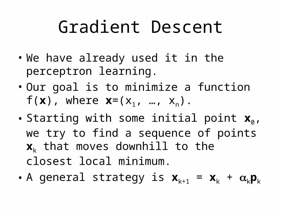
• We have already used it in the perceptron learning.

• Our goal is to minimize a function f(x), where x=(x1, …, xn).

• Starting with some initial point x0, we try to find a sequence of points xk that moves downhill to the closest local minimum.

• A general strategy is xk+1 = xk + kpk

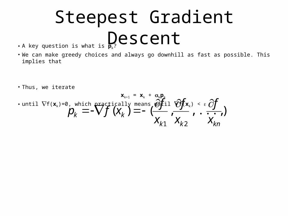
Steepest Gradient Descent• A key question is what is pk?

• We can make greedy choices and always go downhill as fast as possible. This implies that

• Thus, we iterate xk+1 = xk + kpk

• until f(xk)=0, which practically means until f(xk) < ),...,,()(21 knkk

kk x

f

x

f

x

fxfp

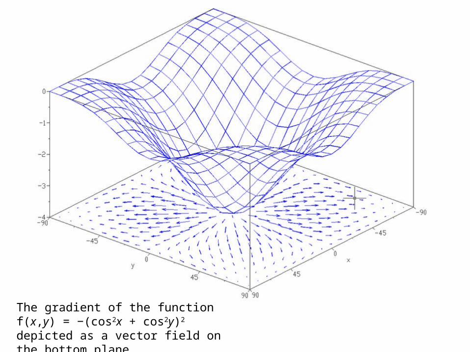
The gradient of the function f(x,y) = −(cos2x + cos2y)2 depicted as a vector field on the bottom plane

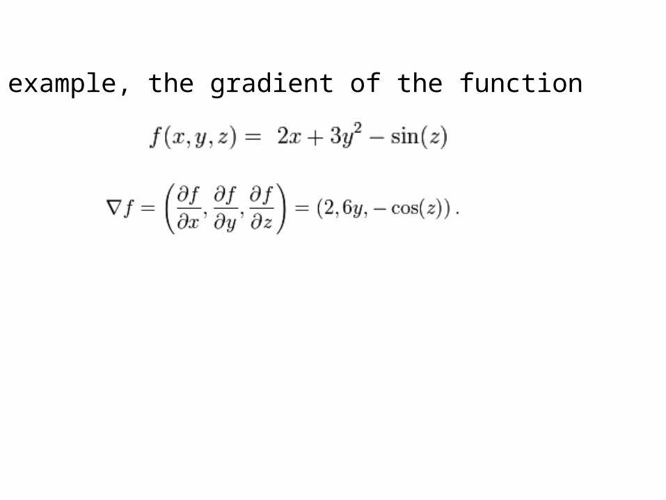
For example, the gradient of the function

is:

6

Recall the Gradient Descent Learning Rule of Perceptron

• Consider linear perceptron without threshold and continuous output (not just –1,1)– y=w0 + w1 x1 + … + wn xn

• Train the wi’s such that they minimize the squared error

E[w1,…,wn] = ½ dD (td-yd)2

where D is the set of training examplesThen wk+1 = wk - kf(wk) = wk - kE(wk)

We wrote wk+1 = wk +wk,

thus wk = - kE(wk)

7

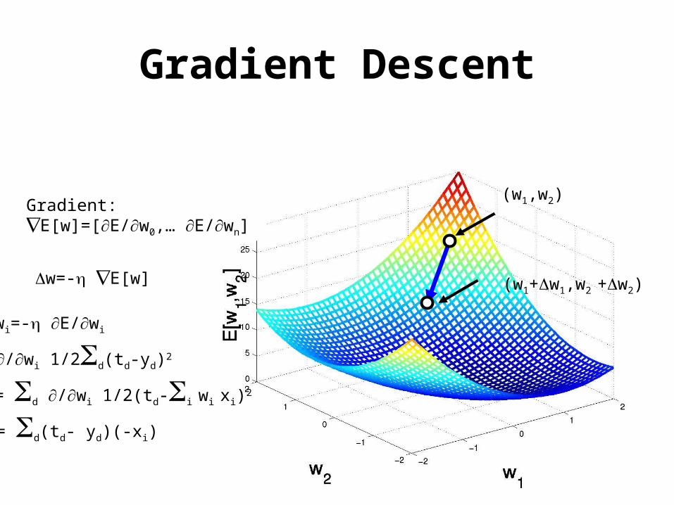
Gradient Descent

Gradient:E[w]=[E/w0,… E/wn]

(w1,w2)

(w1+w1,w2 +w2)w=- E[w]

wi=- E/wi

/wi 1/2d(td-yd)2

= d /wi 1/2(td-i wi xi)2

= d(td- yd)(-xi)

161.326 Stephen Marsland

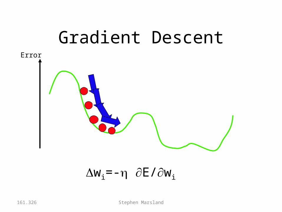
Gradient DescentError

wi=- E/wi

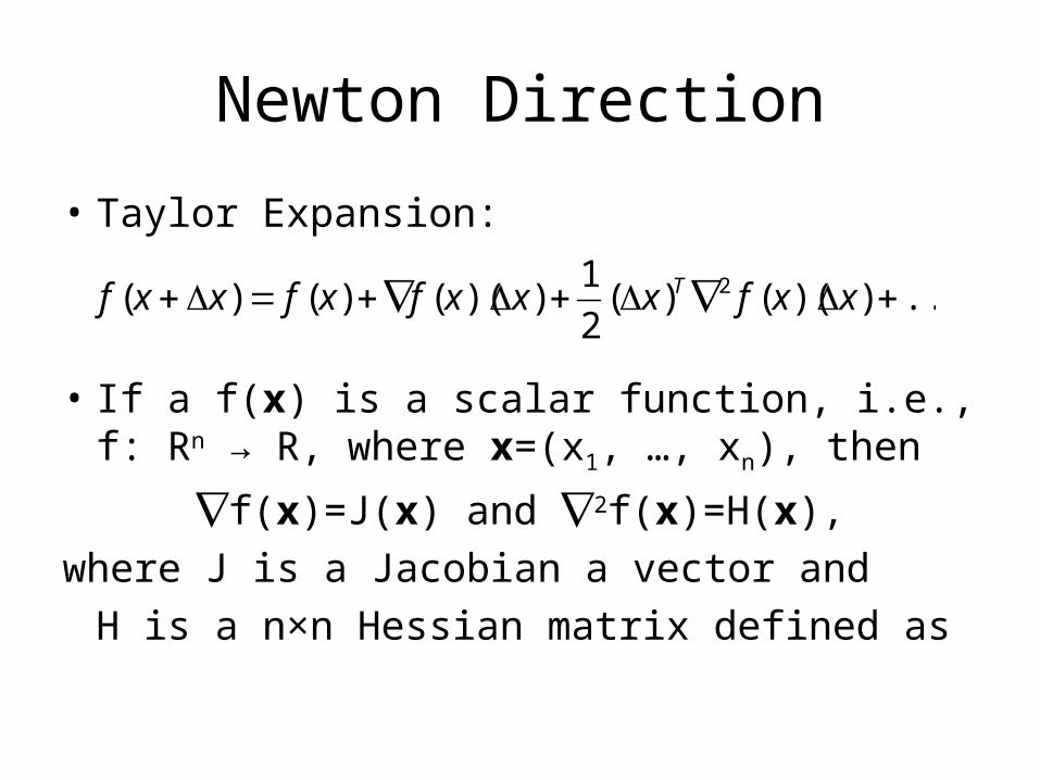
Newton Direction

• Taylor Expansion:

• If a f(x) is a scalar function, i.e., f: Rn → R, where x=(x1, …, xn), then

f(x)=J(x) and 2f(x)=H(x),where J is a Jacobian a vector and

H is a n×n Hessian matrix defined as

...))(()(2

1))(()()( 2 xxfxxxfxfxxf T

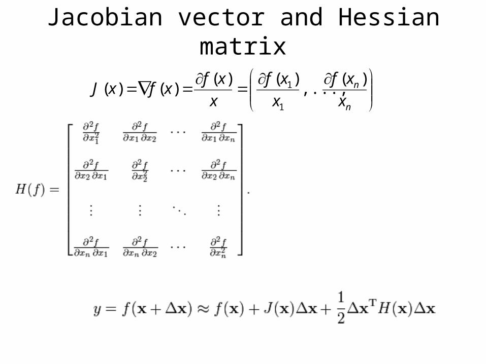
Jacobian vector and Hessian matrix

n

n

x

xf

x

xf

x

xfxfxJ

)(,...,)()(

)()(1

1

Newton Direction

• Since

we obtain

In xk+1 = xk + kpk and the step size is always k=1.

)())(()())(( 112kkkkk xJxHxfxfp

0)()()()(

)(2

1)()()(

xxHxJxfxxfx

xxxHxxJxfxxf

Search Algorithms• Example problem:

Traveling Salesman Problem (TSP), which is introduced on next slides.

• Then we will explore various search strategies and illustrate them on TSP:

1.Exhaustive Search2.Greedy Search3.Hill Climbing4.Simulated Annealing

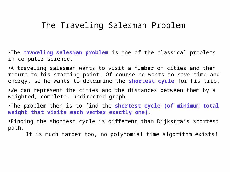
The Traveling Salesman Problem

•The traveling salesman problem is one of the classical problems in computer science.

•A traveling salesman wants to visit a number of cities and then return to his starting point. Of course he wants to save time and energy, so he wants to determine the shortest cycle for his trip.

•We can represent the cities and the distances between them by a weighted, complete, undirected graph.

•The problem then is to find the shortest cycle (of minimum total weight that visits each vertex exactly one).

•Finding the shortest cycle is different than Dijkstra’s shortest path.It is much harder too, no polynomial time algorithm exists!

The Traveling Salesman Problem

• Importance:– Variety of scheduling application can be solved as a

traveling salesmen problem. – Examples:

• Ordering drill position on a drill press. • School bus routing.

– The problem has theoretical importance because it represents a class of difficult problems known as NP-hard problems.

THE FEDERAL EMERGENCY MANAGEMENT AGENCY

• A visit must be made to four local offices of FEMA, going out from and returning to the same main office in Northridge, Southern California.

FEMA traveling salesman Network representation

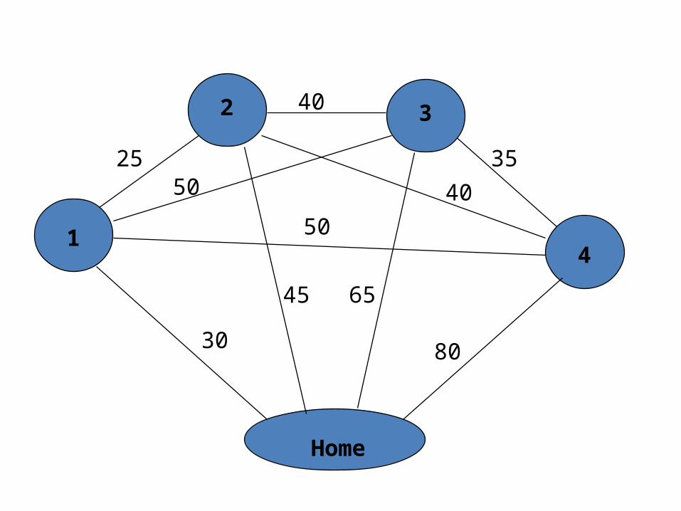
30

25

40

35

80

6545

50

5040

Home

1

2 3

4

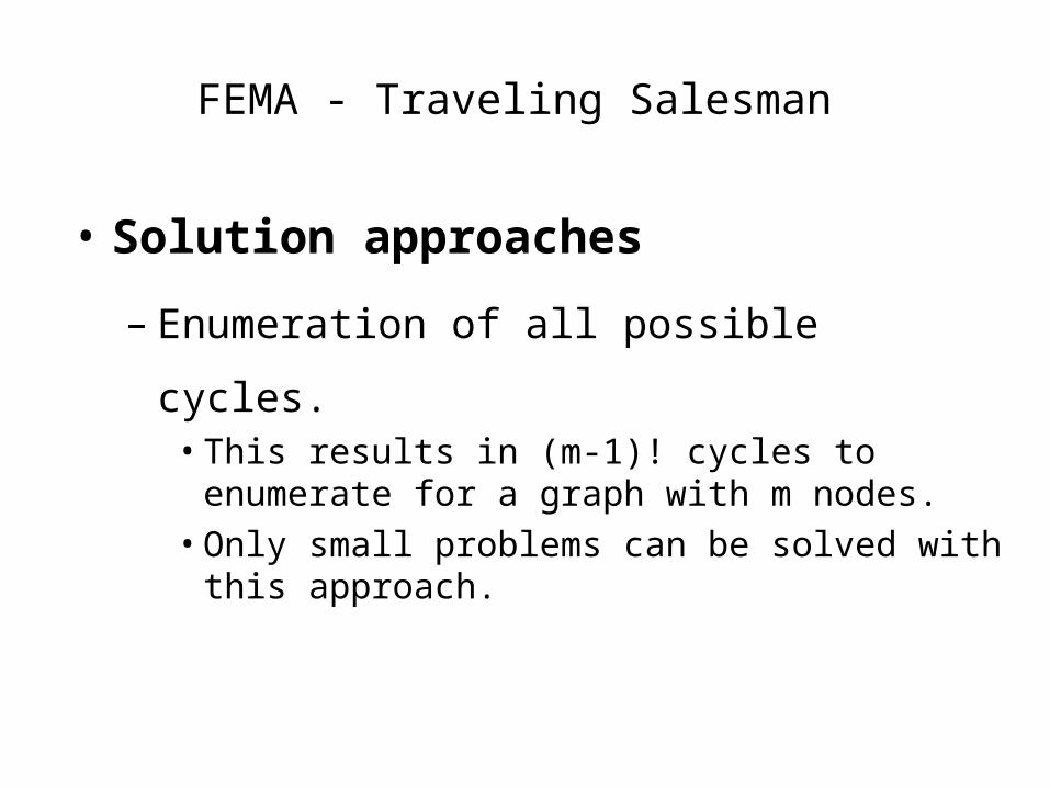
FEMA - Traveling Salesman

• Solution approaches

– Enumeration of all possible cycles.• This results in (m-1)! cycles to enumerate for a graph with m

nodes. • Only small problems can be solved with this approach.

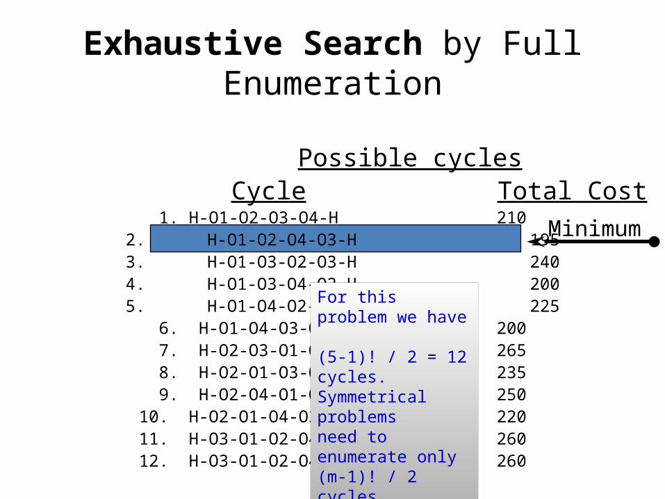
Possible cyclesCycle Total Cost

1. H-O1-O2-O3-O4-H 210 2. H-O1-O2-O4-O3-H 195 3. H-O1-O3-O2-O3-H 240 4. H-O1-O3-O4-O2-H 200 5. H-O1-O4-O2-O3-H 225 6. H-O1-O4-O3-O2-H 200 7. H-O2-O3-O1-O4-H 265 8. H-O2-O1-O3-O4-H 235 9. H-O2-O4-O1-O3-H 25010. H-O2-O1-O4-O3-H 22011. H-O3-O1-O2-O4-H 26012. H-O3-O1-O2-O4-H 260

Minimum

For this problem we have

(5-1)! / 2 = 12 cycles. Symmetrical problemsneed to enumerate only (m-1)! / 2 cycles.

Exhaustive Search by Full Enumeration

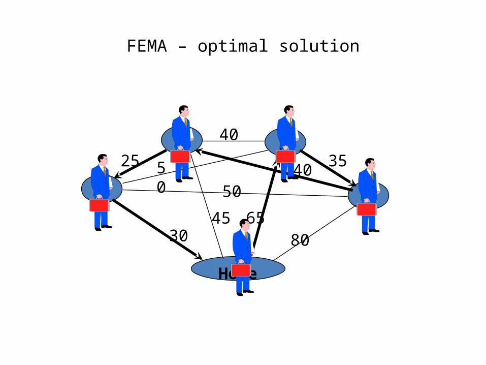
30

25

40

35

806545

5050

40

Home

1

2 3

4

FEMA – optimal solution

The Traveling Salesman Problem

•Unfortunately, no algorithm solving the traveling salesman problem with polynomial worst-case time complexity has been devised yet.

•This means that for large numbers of vertices, solving the traveling salesman problem is impractical.

•In these cases, we can use efficient approximation algorithms that determine a path whose length may be slightly larger than the traveling salesman’s path.

Greedy Search TSP Solution

• Choose the first city arbitrarily, and then repeatedly pick the city that is closest to the current city and that has not been yet visited.

• Stop when all cities have been visited.

Hill Climbing TSP Solution• Choose an initial tour randomly• Then keep swapping pairs of cities if the total

length of tour decreases, i.e., if new dist. traveled < before dist. traveled.

• Stop after a predefined number of swaps or when no swap improved the solution for some time.

• As with greedy search, there is no way to predict how good the solution will be.

Exploration and Exploitation

• Exploration of the search space is like exhaustive search (always trying out new solutions)

• Exploitation of the current best solution is like hill climbing (trying local variants of the current best solution)

• Ideally we would like to have a combination of those two.

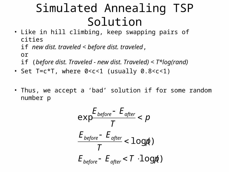
Simulated Annealing TSP Solution• Like in hill climbing, keep swapping pairs of cities

if new dist. traveled < before dist. traveled,orif (before dist. Traveled - new dist. Traveled) < T*log(rand)

• Set T=c*T, where 0<c<1 (usually 0.8<c<1)

• Thus, we accept a ‘bad’ solution if for some random number p

)log(

)log(

exp

pTEE

pT

EE

pT

EE

afterbefore

afterbefore

afterbefore

Search Algorithms Covered1. Exhaustive Search2. Greedy Search3. Hill Climbing4. Simulated Annealing