long-time asymptotics of perturbed - tum m7/analysis

LONG-TIME ASYMPTOTICS OF PERTURBED FINITE-GAP

KORTEWEG–DE VRIES SOLUTIONS

ALICE MIKIKITS-LEITNER AND GERALD TESCHL

Abstract. We apply the method of nonlinear steepest descent to compute the

long-time asymptotics of solutions of the Korteweg–de Vries equation whichare decaying perturbations of a quasi-periodic finite-gap background solution.

We compute a nonlinear dispersion relation and show that the x/t plane splits

into g + 1 soliton regions which are interlaced by g + 1 oscillatory regions,where g + 1 is the number of spectral gaps.

In the soliton regions the solution is asymptotically given by a number of

solitons travelling on top of finite-gap solutions which are in the same isospec-tral class as the background solution. In the oscillatory region the solution

can be described by a modulated finite-gap solution plus a decaying dispersive

tail. The modulation is given by a phase transition on the isospectral torusand is, together with the dispersive tail, explicitly characterized in terms of

Abelian integrals on the underlying hyperelliptic curve.

1. Introduction

Consider the Korteweg–de Vries (KdV) equation

(1.1) Vt(x, t) = 6V (x, t)Vx(x, t)− Vxxx(x, t), (x, t) ∈ R× R,where the subscripts denote differentiation with respect to the corresponding vari-ables.

Following the seminal work of Gardner, Green, Kruskal, and Miura [17], onecan use the inverse scattering transform to establish existence and uniqueness of(real-valued) classical solutions for the corresponding initial value problem withrapidly decaying initial conditions. We refer to, for instance, the monograph byMarchenko [28]. Our concern here are the long-time asymptotics of such solutions.The classical result is that an arbitrary short-range solution of the above type willeventually split into a number of solitons travelling to the right plus a decaying ra-diation part travelling to the left. The first numerical evidence for such a behaviourwas found by Zabusky and Kruskal [37]. The first mathematical results were givenby Ablowitz and Newell [1], Manakov [27], and Sabat [31]. First rigorous results forthe KdV equation were proved by Sabat [31] and Tanaka [33]. Precise asymptoticsfor the radiation part were first formally derived by Zakharov and Manakov [36],by Ablowitz and Segur [2], [32], by Buslaev [6] (see also [5]), and later on rigorouslyjustified and extended to all orders by Buslaev and Sukhanov [7]. A detailed rig-orous proof (not requiring any a priori information on the asymptotic form of the

Date: September 2, 2011.

2000 Mathematics Subject Classification. Primary 35Q53, 37K40; Secondary 35Q15, 37K20.

Key words and phrases. Riemann–Hilbert problem, Korteweg–de Vries equation, Solitons.Research supported by the Austrian Science Fund (FWF) under Grant No. Y330.J. d’Analyse Math. (to appear).

1

2 A. MIKIKITS-LEITNER AND G. TESCHL

solution) was given by Deift and Zhou [8] based on earlier work of Manakov [27] andIts [18] and is now known as the nonlinear steepest descent method for oscillatoryRiemann–Hilbert problems. For an expository introduction to this method appliedto the KdV equation we refer to [20]. For further information on the history of thisproblem we refer to the survey by Deift, Its, and Zhou [9].

In this paper we want to look at the case of solutions which are asymptoticallyclose to a quasi-periodic algebro-geometric finite-gap solution of the KdV equation.In this case the underlying inverse scattering transform was developed only recentlyby Grunert, Egorova, and Teschl [12], [13], [14]. So while the initial value problemfor this class of solutions is well understood, nothing was known about their long-time asymptotics even though the first attempts by Kuznetsov and Mikhaılov [23]date back over 35 years ago. It is the aim of the present paper to fill this gap. Incase of the discrete analog, the Toda lattice (see e.g. [34]), Kamvissis and Teschl[21], [22] (with further extensions by Kruger and Teschl [26]) have recently extendedthe nonlinear steepest descent method for Riemann–Hilbert problem deformationsto Riemann surfaces and used this extension to prove the following result for theToda lattice:

Let g be the genus of the hyperelliptic curve associated with the unperturbedsolution. Then, apart from the phenomenon of the solitons travelling on the quasi-periodic background, the (n, t)-plane contains g + 2 areas where the perturbedsolution is close to a finite-gap solution from the same isospectral torus. In betweenthere are g + 1 regions where the perturbed solution is asymptotically close to amodulated lattice which undergoes a continuous phase transition (in the Jacobianvariety) and which interpolates between these isospectral solutions. In the specialcase of the free lattice (g = 0) the isospectral torus consists of just one point andthe known results are recovered. Both the solutions in the isospectral torus andthe phase transition were explicitly characterized in terms of Abelian integrals onthe underlying hyperelliptic curve.

In the present paper we will use this extension for Riemann–Hilbert problems onRiemann surfaces to prove an analog result for the KdV equation to be formulatedin the next section.

2. Main results

To set the stage we will choose a quasi-periodic algebro-geometric finite-gapbackground solution Vq(x, t) of the KdV equation (cf. the next section) plus anothersolution V (x, t) of the KdV equation such that

(2.1)

∫ +∞

−∞(1 + |x|)7(|V (x, t)− Vq(x, t)|)dx <∞

for all t ∈ R. We remark that such solutions exist which can be shown by solvingthe associated Cauchy problem via the inverse scattering transform [12].

To fix our background solution Vq, let us consider a hyperelliptic Riemann surfaceKg of genus g ∈ N0 with real moduli E0, E1, . . . , E2g. Then we choose a Dirichletdivisor Dµ(x,t) and introduce

(2.2)z(p, x, t) = ΞE0

− AE0(p) + αE0

(Dµ(x,t)) ∈ Cg,

αE0(Dµ(x,t)) = αE0

(Dµ) +x

2πU0 + 12

t

2πU2,

ASYMPTOTICS OF PERTURBED FINITE-GAP KDV SOLUTIONS 3

where AE0(αE0

) is Abel’s map (for divisors), and ΞE0, U0, and U2 are some

constants defined in detail in Section 3 below. Then our background solution isgiven in terms of Riemann theta functions (cf. (3.13)) by

(2.3)

Vq(x, t) = E0 +

g∑j=1

(E2j−1 + E2j − 2µj(x, t))

= E0 +

g∑j=1

(E2j−1 + E2j − 2λj)− 2∂2x ln θ

(z(p∞, x, t)

),

where λj ∈ (E2j−1, E2j), j = 1, . . . , g.In order to state our main result, we begin by recalling that the perturbed KdV

solution V (x, t), x ∈ R, for fixed t ∈ R, is uniquely determined by its scatteringdata, that is, by the right reflection coefficient R+(λ, t), λ ∈ σ(Hq), and the eigen-values ρk ∈ R\σ(Hq), k = 1, . . . , N , together with the corresponding right normingconstants γ+,k(t) > 0, k = 1, . . . , N . Here

(2.4) σ(Hq) =

g−1⋃j=0

[E2j , E2j+1] ∪ [E2g,∞)

denotes the finite-band spectrum of the underlying background Lax operator

(2.5) Hq(t) = −∂2x + Vq(x, t).

The relation between the energy λ of the underlying Lax operator Hq and thepropagation speed at which the corresponding parts of the solutions of the KdVequation travel is given by

(2.6) v(λ) =x

t,

where

(2.7) v(λ) = limε→0

−12 Re(i∫ (λ+iε,+)

E0ωp∞,2

)Re(i∫ (λ+iε,+)

E0ωp∞,0

) ,

and can be regarded as a nonlinear analog of the classical dispersion relation. Hereωp∞,0 and ωp∞,2 are Abelian differentials of the second kind on the underlyingRiemann surface defined in (3.15) and (3.16). We will show in Section 5 that v isa decreasing homeomorphism of R and we will denote its inverse by ζ(v).

Furthermore, we define the limiting KdV solution Vl,v(x, t) via the relation∫ ∞x

(Vl,v − Vq)(y, t)dy =−∑

ρj<ζ(v)

4i

∫ ρj

E(ρj)

ωp∞,0 +1

π

∫C(v)

log(1− |R|2)ωp∞,0

+ 2∂x ln

(θ(z(p∞, x, t) + δ(v)

)θ(z(p∞, x, t)

) ), v = min(v, x/t),(2.8)

with

δ`(v) = −2∑

ρj<ζ(v)

AE(ρj),`(ρj) +1

2πi

∫C(v)

log(1− |R|2)ζ`,

where R = R+(λ, t) is the associated reflection coefficient and ζ` is a canonical basisof holomorphic differentials. Moreover, C(v) is a contour on the Riemann surfaceobtained by taking the part of the spectrum σ(Hq) which is to the left of ζ(v) and


lifting it to the Riemann surface (oriented such that the upper sheet lies to its left).Here we have also identified ρj with its lift to the upper sheet and E(ρj) denotesthe branch point closest to ρj . If v = x/t we set Vl(x, t) = Vl,x/t(x, t).

Then our main result concerning the long-time asymptotics in the soliton regionis given by the following theorem:

Theorem 2.1. Assume V (x, t) is a classical solution of the KdV equation (1.1)satisfying

(2.9)

∫ +∞

−∞(1 + |x|1+n)(|V (x, t)− Vq(x, t)|)dx <∞,

for some integer n ≥ 1 and abbreviate by ck = v(ρk) the velocity of the k’th soliton.Then the asymptotics in the soliton region, (x, t)| ζ(x/t) ∈ R\σ(Hq), are thefollowing:

Let ε > 0 be sufficiently small such that the intervals [ck − ε, ck + ε], 1 ≤ k ≤ N ,are disjoint and lie inside v(R\σ(Hq)).

If |xt − ck| < ε for some k, the solution is asymptotically given by a one-solitonsolution on top of the limiting solution:

(2.10)

∫ ∞x

(V − Vl,ck)(y, t)dy = −2∂

∂xlog(cl,k(x, t)

)+O(t−n),

respectively

(2.11) (V − Vl,ck)(x, t) = 2∂2

∂x2log(cl,k(x, t)

)+O(t−n),

where

(2.12) cl,k(x, t) = 1 + γk

∫ ∞x

ψl,ck(ρk, y, t)2dy

and

(2.13)

γk = γk

(θ(z(ρk, 0, 0) + δ(ck))

θ(z(ρk, 0, 0))

)2 ∏ρj<ζ(ck)

exp

(2

∫ ρk

E0

ωρj ρ∗j

) ·· exp

(−1

πi

∫C(ck)

log(1− |R|2)ωρk p∞

).

Here ψl,v(p, x, t) denotes the Baker–Akhiezer function corresponding to the limitingKdV solution Vl,v(x, t) and ωp q denotes the Abelian differential of the third kindwith poles at p and q.

If |xt − ck| ≥ ε, for all k, the solution is asymptotically close to this limitingsolution:

(2.14)

∫ ∞x

(V − Vl)(y, t)dy = O(t−n),

respectively

(2.15) V (x, t) = Vl(x, t) +O(t−n).

In particular, we see that the solution splits into a sum of independent solitonswhere the presence of the other solitons and the radiation part corresponding tothe continuous spectrum manifests itself in phase shifts given by (2.13). Moreover,


observe that in the periodic case considered here one can have a stationary soliton(see the discussion in Section 5).

The proof will be given at the end of Section 5.

Theorem 2.2. Assume V (x, t) is a classical solution of the KdV equation (1.1)satisfying (2.1) and let Dj be the sector Dj = (x, t) : ζ(x/t) ∈ [E2j +ε, E2j+1−ε]for some ε > 0. Then the asymptotic is given by

(2.16)

∫ +∞

x

(V − Vl)(y, t)dy = 4

√i

φ′′(zj)tRe(β(x, t)

)Λν1(zj) +O(t−α),

respectively(2.17)

(V −Vl)(x, t) = 4

√i

φ′′(zj)t

[Im(β(x, t)

)−iRe

(β(x, t)

) g∑k=1

g∑`=1

ck`(ν)ζk(zj)]+O(t−α)

for any 1/2 < α < 1 uniformly in Dj as t→∞. Here

(2.18) φ(p) = −24i

∫ p

p0

ωp∞,2 − 2ix

t

∫ p

p0

ωp∞,0

is the phase function,

(2.19)φ′′(zj)

i= −

12∏gk=0,k 6=j(zj − zk)

iR1/22g+1(zj)

> 0,

(where R1/22g+1(z) the square root of the underlying Riemann surface Kg and we

identify zj with its lift to the upper sheet),

(2.20) Λν1(zj) = ωp∞,0(zj)−

g∑k=1

g∑`=1

ck`(ν)αg−1(ν`)ζk(zj),

with ωp∞,0 an Abelian differential of the second kind with a second order pole atp∞ (cf. eq. (3.15)), and ω(p) denoting the value of a differential evaluated at p inthe chart given by the canonical projection, and ck`(ν), αg−1(ν`) some constantsdefined in (6.24), (6.34), respectively. Moreover,

β(x, t) =√νei(π/4−arg(R(zj))+arg(Γ(iν))+2να(zj)

)(φ′′(zj)i

)−iν

e−tφ(zj)t−iν ·

·θ(z(zj , 0, 0)

)θ(z(zj , x, t) + δ(x/t)

) θ(z(z∗j , x, t) + δ(x/t))

θ(z(z∗j , 0, 0)

) ·

· exp

(−

∑ρk<ζ(x/t)

∫ ρk

E(ρk)

ωzj z∗j +1

2πi

∫C(x/t)

log( 1− |R|2

1− |R(zj)|2)ωzj z∗j

),(2.21)

where Γ(z) is the gamma function, ωzj z∗j an Abelian differential of the third kind

defined in (3.21),

(2.22) ν = − 1

2πlog(1− |R(zj)|2

)> 0,

and α(zj) is a constant defined in (6.9).

The proof of this theorem will be given in Section 6 of this paper.Finally, note that if q(x, t) solves the KdV equation, then so does q(−x,−t).

Therefore it suffices to investigate the case t→∞.


3. Algebro-geometric quasi-periodic finite-gap solutions

This section presents some well-known facts on the class of algebro-geometricquasi-periodic finite-gap solutions, that is the class of stationary solutions of theKdV hierarchy, since we want to choose our background solution Vq from that class.We will use the same notation as in [16], where we also refer to for proofs. As areference for Riemann surfaces in this context we recommend [15].

To set the stage let Kg be the Riemann surface associated with the followingfunction

(3.1) R1/22g+1(z) = i

2g∏j=0

√z − Ej , E0 < E1 < · · · < E2g,

where g ∈ N0 and Ej2gj=0 is a set of real numbers. Here√. denotes the standard

root with branch cut along (0,∞). We extend R1/22g+1(z) to the branch cuts by

setting R1/22g+1(z) = limε↓0R

1/22g+1(z + iε) for z ∈ C\Π. Hence we have

(3.2)

R1/22g+1(z) = |R1/2

2g+1(z)| ·

(−1)g+1 for z ∈ (−∞, E0),(−1)g+j i for z ∈ (E2j , E2j+1), j = 0, . . . , g − 1,(−1)g+j for z ∈ (E2j+1, E2j+2), j = 0, . . . , g − 1,i for z ∈ (E2g,∞).

Kg is a compact, hyperelliptic Riemann surface of genus g.

A point on Kg is denoted by p = (z,±R1/22g+1(z)) = (z,±), z ∈ C, or p∞ =

(∞,∞), and the projection onto C ∪ ∞ by π(p) = z. The points (Ej , 0), 0 ≤j ≤ 2g ∪ (∞,∞) ⊆ Kg are called branch points and the sets

(3.3) Π± = (z,±R1/22g+1(z)) | z ∈ C \

g−1⋃j=0

[E2j , E2j+1] ∪ [E2g,∞) ⊂ Kg

are called upper, lower sheet, respectively.Next we will introduce the representatives aj , bjgj=1 of a canonical homology

basis for Kg. For aj we start near E2j−1 on Π+, surround E2j thereby changing toΠ− and return to our starting point encircling E2j−1 again changing sheets. Forbj we choose a cycle surrounding E0, E2j−1 counterclockwise (once) on Π+. Thecycles are chosen such that their intersection matrix reads

(3.4) ai aj = bi bj = 0, ai bj = δi,j , 1 ≤ i, j ≤ g.The corresponding canonical basis ζjgj=1 for the space of holomorphic differ-

entials can be constructed by

(3.5) ζj =

g∑k=1

cj(k)πk−1dπ

R1/22g+1

,

where the constants cj(k), j, k = 1, . . . , g are given by

(3.6) cj(k) = C−1jk , Cjk =

∫ak

πj−1dπ

R1/22g+1

= 2

∫ E2k

E2k−1

zj−1dz

R1/22g+1(z)

∈ R.

The differentials fulfill

(3.7)

∫ak

ζj = δk,j ,

∫bk

ζj = τk,j , τk,j = τj,k, j, k = 1, . . . , g.


Let us now pick g numbers (the Dirichlet eigenvalues)

(3.8) (µj)gj=1 = (µj , σj)

gj=1

whose projections lie in the spectral gaps, that is, µj ∈ [E2j−1, E2j ], j = 1, . . . , g.Associated with these numbers is the divisor

(3.9) Dµ(p) =

1 p = µj , j = 1, . . . , g,0 else

and we can define g numbers (µj(x, t))gj=1 = (µj(x, t), σj(x, t))

gj=1 via Jacobi’s

inversion theorem by setting

(3.10) αE0(Dµ(x,t)) = αE0

(Dµ) +x

2πU0 + 12

t

2πU2

such that µj(0, 0) = µj . Here U0 and U2 denote the b-periods of the Abeliandifferentials ωp∞,0 and ωp∞,2, respectively, defined below, and AE0

(αE0) is Abel’s

map (for divisors). The hat indicates that we regard it as a (single-valued) map

from Kg (the fundamental polygon associated with Kg by cutting along the a andb cycles) to Cg.

Next we introduce

(3.11) z(p, x, t) = ΞE0− AE0

(p) + αE0(Dµ(x,t)) ∈ Cg,

where ΞE0is the vector of Riemann constants

(3.12) ΞE0,j =j +

∑gk=1 τj,k2

, j = 1, . . . , g.

By θ(z) we denote the Riemann theta function associated with Kg defined by

(3.13) θ(z) =∑m∈Zg

exp 2πi

(〈m, z〉+

〈m, τ m〉2

), z ∈ Cg.

Note that the function θ(z(p, x, t)) has precisely g zeros µj(x, t). This follows fromRiemann’s vanishing theorem (cf. [34, Theorem A.13]).

Introduce the time-dependent Baker–Akhiezer function(3.14)

ψq(p, x, t) =θ(z(p, x, t)

)θ(z(p∞, x, t)

) θ(z(p∞, 0, 0))

θ(z(p, 0, 0)

) exp(− ix

∫ p

E0

ωp∞,0 − 12it

∫ p

E0

ωp∞,2

).

Here ωp∞,0 and ωp∞,2 are normalized Abelian differentials of the second kind witha single pole at p∞ and principal part w−2dw and w−4dw in the chart w(p) =±iz−1/2 for p = (z,±), respectively. The Abelian differentials are normalized tohave vanishing aj periods and have the following expressions

(3.15) ωp∞,0 =1

2i

∏gj=1(π − λj)

R1/22g+1

dπ,

with λj ∈ (E2j−1, E2j), j = 1, . . . , g, and

(3.16) ωp∞,2 =1

2i

∏gj=0(π − λj)

R1/22g+1

dπ,


where λj , j = 0, . . . , g, have to be chosen such that they fulfill∑gj=0 λj = 1

2

∑2gj=0Ej .

We also remark

(3.17) ψq(p, x, t)ψq(p∗, x, t) =

g∏j=1

z − µj(x, t)z − µj

, p = (z,±).

Then our background KdV solution is given by

(3.18) Vq(x, t) = E0 +

g∑j=1

(E2j−1 + E2j − 2λj)− 2∂2x ln θ

(z(p∞, x, t)

).

The Abelian differentials of the third kind ωq1 q2 , with simple poles at q1 andq2, corresponding residues +1 and −1, vanishing a-periods, and holomorphic onKg \ q1, q2, are explicitly given by ([16, Appendix B])

ωp1 p2 =(R1/2

2g+1 +R1/22g+1(p1)

2(π − π(p1)

) −R

1/22g+1 +R

1/22g+1(p2)

2(π − π(p2)

) + Pp1 p2(z)) dπ

R1/22g+1

,(3.19)

ωp1 p∞ =(R1/2

2g+1 +R1/22g+1(p1)

2(π − π(p1)

) + Pp1 p∞(z)) dπ

R1/22g+1

,(3.20)

where p1, p2 ∈ Kg \ p∞ and Pp1 p2(z) and Pp1 p∞(z) are polynomials of degreeg − 1 which have to be determined from the normalization

∫a`ωp1 p2 = 0 and∫

a`ωp1 p∞ = 0, respectively. In particular,

(3.21) ωpp∗ =(R1/2

2g+1(p)

π − π(p)+ Ppp∗(π)

) dπ

R1/22g+1

.

We will also need the Blaschke factor

(3.22) B(p, ρ) = exp(∫ p

E0

ωρ ρ∗)

= exp(∫ ρ

E(ρ)

ωp p∗), π(ρ) ∈ R,

where E(ρ) is E0 if ρ < E0, either E2j−1 or E2j if ρ ∈ (E2j−1, E2j), 1 ≤ j ≤ g. Itis a multivalued function with a simple zero at ρ and simple pole at ρ∗ satisfying|B(p, ρ)| = 1, p ∈ ∂Π+. It is real-valued for π(p) ∈ (−∞, E0) and satisfies

(3.23) B(E0, ρ) = 1 and B(p∗, ρ) = B(p, ρ∗) = B(p, ρ)−1

(see e.g., [35]).The Baker–Akhiezer function is a meromorphic function on Kg \ p∞ with an

essential singularity at p∞. The two branches are denoted by

(3.24) ψq,±(z, x, t) = ψq(p, x, t), p = (z,±),

and it satisfies

Hq(t)ψq(p, x, t) = π(p)ψq(p, x, t),

d

dtψq(p, x, t) = Pq,2(t)ψq(p, x, t).(3.25)

Here

Hq(t) = ∂2x + Vq(., t),

Pq,2(t) = −4∂3x + 6Vq(., t)∂x + 3Vq,x(., t),(3.26)


are the operators from the Lax pair for the KdV equation, that is,

(3.27)d

dtHq(t) = Hq(t)Pq,2(t)− Pq,2(t)Hq(t).

It is well known that the spectrum of Hq(t) is time independent and consists ofg + 1 bands

(3.28) σ(Hq(t)) =

g−1⋃j=0

[E2j , E2j+1] ∪ [E2g,∞).

For further information and proofs we refer to [16].

4. The Inverse scattering transform and the Riemann–Hilbertproblem

In this section we recall some basic facts from the inverse scattering transformfor our setting. For further background and proofs we refer to [4], [14], and [12](see also [29]).

Let ψq,±(z, x, t) be the branches of the Baker–Akhiezer function defined in theprevious section. Let ψ±(z, x, t) be the Jost functions for the perturbed problem

(4.1)(− ∂2

x + V (x, t))ψ±(z, x, t) = zψ±(z, x, t),

defined by the asymptotic normalization

(4.2) limx→±∞

e∓ixk(z)(ψ±(z, x, t)− ψq,±(z, x, t)

)= 0,

where k(z) denotes the quasimomentum map

(4.3) k(z) = −∫ p

E0

ωp∞,0, p = (z,+).

The asymptotics of the two projections of the Jost function are (cf. [29, Theo-rem 2.3])

(4.4) ψ±(z, x, t) = ψq,±(z, x, t)(

1∓∫ ±∞x

(V − Vq)(y, t)dy1

2i√z

+ o(1/√z)),

as z → ∞. We will assume that the poles of the Baker–Akhiezer function µk areall different from the eigenvalues ρj without loss of generality (otherwise just shiftthe base point (x0, t0) = (0, 0)).

One has the scattering relations

(4.5) T (z)ψ∓(z, x, t) = ψ±(z, x, t) +R±(z)ψ±(z, x, t), z ∈ σ(Hq),

where T (z), R±(z) are the transmission respectively reflection coefficients. Hereψ±(z, x, t) is defined such that ψ±(z, x, t) = limε↓0 ψ±(z + iε, x, t), z ∈ σ(Hq). If

we take the limit from the other side we have ψ±(z, x, t) = limε↓0 ψ±(z − iε, x, t).The transmission and reflection coefficients have the following well-known prop-

erties:

Lemma 4.1. The transmission coefficient T (z) has a meromorphic extension toC\σ(Hq) with simple poles at the eigenvalues ρj. The residues of T (z) are given by

(4.6) Resρj T (z) =2R

1/22g+1(ρj)∏g

k=1(ρj − µk)

γ±,j

c±1j

,


where

(4.7) γ−1±,j =

∫ ∞−∞|ψ±(ρj , y, t)|2dy

are referred to as norming constants and ψ−(ρj , x, t) = cjψ+(ρj , x, t).Moreover,

(4.8) T (z)R+(z) + T (z)R−(z) = 0, |T (z)|2 + |R±(z)|2 = 1.

In particular one reflection coefficient, say R(z) = R+(z), and one set of normingconstants, say γj = γ+,j , suffices.

We will define a sectionally meromorphic vector on the Riemann surface Kg asfollows:

(4.9) m(p, x, t) =

(T (z) ψ−(z,x,t)

ψq,−(z,x,t)ψ+(z,x,t)ψq,+(z,x,t)

), p = (z,+)(

ψ+(z,x,t)ψq,+(z,x,t) T (z) ψ−(z,x,t)

ψq,−(z,x,t)

), p = (z,−)

.

We are interested in the jump condition of m(p, x, t) on Σ, the boundary of Π±(oriented counterclockwise when viewed from top sheet Π+). It consists of twocopies Σ± of σ(Hq) which correspond to non-tangential limits from p = (z,+) with±Im(z) > 0, respectively to non-tangential limits from p = (z,−) with ∓Im(z) > 0.

To formulate our jump condition we use the following convention: When repre-senting functions on Σ, the lower subscript denotes the non-tangential limit fromΠ+ or Π−, respectively,

(4.10) m±(p0) = limΠ±3p→p0

m(p), p0 ∈ Σ.

Using the notation above implicitly assumes that these limits exist in the sense thatm(p) extends to a continuous function on the boundary away from the band edges.

Moreover, we will also use symmetries with respect to the sheet exchange map

(4.11) p∗ =

(z,∓) for p = (z,±),

p∞ for p = p∞,

and complex conjugation

(4.12) p =

(z,±) for p = (z,±) 6∈ Σ,

(z,∓) for p = (z,±) ∈ Σ,

p∞ for p = p∞.

In particular, we have p = p∗ for p ∈ Σ.Note that we have m±(p) = m∓(p∗) for m(p) = m(p∗) (since ∗ reverses the

orientation of Σ) and m±(p) = m±(p∗) for m(p) = m(p).Note that we have the following asymptotic behavior for m(p, x, t) near p∞:

(4.13) m(p) =(1 1

)− 1

2i√z

∫ ∞x

(V −Vq)(y, t)dy(−1 1

)+ o( 1√

z

), p = (z,±)

for p near p∞. Here we made use of (4.4) and

(4.14) T (z) = 1 +1

2i√z

∫ ∞−∞

(V − Vq)(y, t)dy + o( 1√

z

)(cf. [29, Corollary 3.7]).

We are now ready to derive the main vector Riemann–Hilbert problem:


Theorem 4.2 (Vector Riemann–Hilbert problem). Let S+(H(0)) = R(λ), λ ∈σ(Hq); (ρj , γj), 1 ≤ j ≤ N the right scattering data of the operator H(0). Thenm(p) = m(p, x, t) defined in (4.9) is meromorphic away from Σ and satisfies:

(i) The jump condition(4.15)

m+(p) = m−(p)J(p), J(p) =

(1− |R(p)|2 −R(p)Θ(p, x, t)e−tφ(p)

R(p)Θ(p, x, t)etφ(p) 1

),

for p ∈ Σ,(ii) the divisor

(4.16) (m1) ≥ −Dµ(x,t)∗ −Dρ, (m2) ≥ −Dµ(x,t) −Dρ∗

and pole conditions(4.17)(

m1(p) +−2R

1/22g+1(ρj)∏g

k=1(ρj − µk)

γjπ(p)− ρj

ψq(p, x, t)

ψq(p∗, x, t)m2(p)

)≥ −Dµ(x,t)∗ , near ρj ,

( −2R1/22g+1(ρj)∏g

k=1(ρj − µk)

γjπ(p)− ρj

ψq(p∗, x, t)

ψq(p, x, t)m1(p) +m2(p)

)≥ −Dµ(x,t), near ρ∗j ,

(iii) the symmetry condition

(4.18) m(p∗) = m(p)

(0 11 0

)(iv) and the normalization

(4.19) m(p∞) =(1 1

).

Here (f) denotes the divisor of f and

(4.20) Dρ =∑j

Dρj , Dρ∗ =∑j

Dρ∗j .

denotes the divisor corresponding to the points ρj ≡ (ρj ,+) ∈ Kg. The phase φ isgiven by

(4.21) φ(p,x

t) = −24i

∫ p

p0

ωp∞,2 − 2ix

t

∫ p

p0

ωp∞,0 ∈ iR for p ∈ Σ.

Moreover, we have set

(4.22) Θ(p, x, t) =θ(z(p, x, t))

θ(z(p, 0, 0))

θ(z(p∗, 0, 0))

θ(z(p∗, x, t))

such thatψq(p, x, t)

ψq(p∗, x, t)= Θ(p, x, t)etφ(p).

Here we have extended our definition of R to Σ such that it is equal to R(z)

on Σ+ and equal to R(z) on Σ−. In particular, the condition on Σ+ is just the

complex conjugate of the one on Σ− since we have R(p∗) = R(p) and m±(p∗, x, t) =

m±(p, x, t) for p ∈ Σ.


Proof. The jump condition follows by using (4.5) and (4.8). By Riemann’s vanish-ing theorem (cf. [34, Theorem A.13]) the Baker–Akhiezer function ψq has simplezeros at µj(x, t) and simple poles at µj , j = 1, . . . , g. Moreover, the transmissioncoefficient T (z) has simple poles at the eigenvalues ρj , j = 1, . . . , N . Thus thedivisor conditions (4.16) are indeed fulfilled. The pole conditions follow from thefact that the transmission coefficient T (z) is meromorphic in C\σ(Hq) with simplepoles at ρj and its residues are given by (4.6). The symmetry condition (4.18)obviously holds by the definition of the function m(p). The normalization (4.19) isimmediately clear from (4.13).

We note that the symmetry condition is in fact crucial to guarantee that thesolution of this vector Riemann–Hilbert problem is unique.

Theorem 4.3. The vector m(p) defined in (4.9) is the only solution of the vectorRiemann–Hilbert problem (4.15)–(4.19).

Proof. The argument is similar to [22, Thm. B.1]. It suffices to show that the corre-sponding vanishing Riemann–Hilbert problem, where the normalization condition(4.19) is replaced by m(p∞) =

(0 0

), has only the trivial solution.

Let m be some solution of the vanishing Riemann–Hilbert problem. We wantto apply Cauchy’s integral theorem to m(p)m†(p∗). To handle the poles of mwe will multiply it by a meromorphic differential dΩ which has zeros at µ and

µ∗ and a simple pole at p∞ such that finally the differential m(p)m†(p∗)dΩ(p) is

holomorphic away from the contour. Here m† denotes the adjoint (transpose andcomplex conjugate) vector of m.

More precisely, let

(4.23) dΩ =

∏gj=1(π − µj)

−R1/22g+1

dπ

and note that −(∏

j(z−µj))R−1/22g+1(z) is a Herglotz function. That is, it has positive

imaginary part in the upper half-plane (and it is purely imaginary on σ(Hq)). Hence

m(p)mT (p)dΩ(p) will be positive on Σ.Next, consider the integral

(4.24) 0 =

∫D

m(p)m†(p∗)dΩ(p),

where D is a ∗-invariant contour consisting of two loops on the upper and on thelower sheet encircling none of the poles ρj , ρ

∗j . We first deform D to a ∗-invariant

contour consisting of several parts: Two pieces D± wrapping around the ± side ofΣ plus a number of small circles D+,j , D−,j around the poles ρj , ρ

∗j , respectively.

Then the contribution from Σ is given by∫Σ

m(p)m†(p∗)dΩ(p) =

∫Σ

(m+(p)m†−(p∗) + m−(p)m†+(p∗)

)dΩ(p)

=

∫Σ

m−(p)(J(p) + J†(p∗))m†−(p∗)dΩ(p) ≥ 0(4.25)


and the contribution from the poles is given by∫∪Nj=1(D+,j∪D−,j)

m(p)m†(p∗)dΩ(p)

=

N∑j=1

(Resρj m(p)m†(p∗)dΩ(p) + Resρ∗j m(p)m†(p∗)dΩ(p)

)

= 2

N∑j=1

Resρj m(p)m†(p∗)dΩ(p).(4.26)

To compute the residues we use the pole conditions (4.17) which imply (using(3.17))

Resρj m(p)m†(p∗)dΩ(p) =2γj∏g

k=1(ρj − µ0k)2

ψq(ρj)2m2(ρj)

2 ≥ 0.

In particular, both contributions to the integral (4.24) are non-negative and thusboth must vanish. It follows from the that m = 0 vanishes along Σ and consequentlym(p) = 0 as desired.

We will also need another asymptotic relation

(4.27) m1 ·m2 = 1 + (V − Vq)(x, t)1

2z+ o(z−1).

which is immediate from the following well-known result.

Lemma 4.4. We have

(4.28) T (z)ψ−(z, x, t)

ψq,−(z, x, t)

ψ+(z, x, t)

ψq,+(z, x, t)= 1 +

1

2(V − Vq)(x, t)

1

z+ o(z−1).

Proof. We will use the following representation of the Jost solutions

(4.29) ψ±(z, x, t) = ψq,±(z, x, t) exp(∓∫ ±∞x

(m±(z, y, t)−mq,±(z, y, t)

)dy),

where

m±(z, x, t) = ±ψ′±(z, x, t)

ψ±(z, x, t), mq,±(z, x, t) = ±

ψ′q,±(z, x, t)

ψq,±(z, x, t)

are the Weyl–Titchmarsh functions. Here the prime denotes differentiation withrespect to x. Using the expansion of the Weyl m-functions (cf. [29, Lemma 6.1])and the one for log T (z) (cf. [29, Theorem 6.2]) for z →∞ proves the claim.

For our further analysis it will be convenient to rewrite the pole conditions asjump conditions following the idea of Deift, Kamvissis, Kriecherbauer, and Zhou[11]. For that purpose we choose ε so small that the discs |π(p)− ρj | < ε are insidethe upper sheet Π+ and do not intersect with the spectral bands. Then redefinem(p) in a neighborhood of ρj respectively ρ∗j in the following way:

(4.30) m(p) =

m(p)

(1 0

γj(p,x,t)π(p)−ρj 1

), |π(p)−ρj |<ε

p∈Π+,

m(p)

(1

γj(p∗,x,t)

π(p)−ρj0 1

), |π(p)−ρj |<ε

p∈Π−,

m(p), else,


where γj(p, x, t) is a function which is analytic in 0 < |π(p)− ρj | < ε, p ∈ Π+ andsatisfies

limp→ρj

γj(p, x, t)ψq(p

∗, x, t)

ψq(p, x, t)=

2R1/22g+1(ρj)∏g

k=1(ρj − µk)γj .

For example, we can choose

γj(p, x, t) =−2R

1/22g+1(ρj)∏g

k=1(ρj − µk)

ψq(p, x, t)

ψq(p∗, x, t)γj

or

γj(p, x, t) =−2R

1/22g+1(ρj)∏g

k=1(π(p)− µk)

ψq(p, x, t)

ψq(p∗, x, t)γj .

Lemma 4.5. Suppose m(p) is redefined as in (4.30). Then m(p) is meromor-phic away from Σ and satisfies (4.15), (4.18), (4.19), the divisor conditions changeaccording to

(4.31) (m1) ≥ −Dµ(x,t)∗ , (m2) ≥ −Dµ(x,t)

and the pole conditions are replaced by the jump conditions

(4.32)

m+(p) = m−(p)

(1 0

γj(p,x,t)π(p)−ρj 1

), p ∈ Σε(ρj),

m+(p) = m−(p)

(1 −γj(p

∗,x,t)π(p)−ρj

0 1

), p ∈ Σε(ρ

∗j ),

where

(4.33) Σε(p) = q ∈ Π± : |π(q)− z| = ε, p = (z,±),

is a small circle around p on the same sheet as p. It is oriented counterclockwiseon the upper sheet and clockwise on the lower sheet.

Proof. Everything except for the pole conditions follows as in the proof of Theo-rem 4.2. That the pole conditions (4.17) are indeed replaced by the jump conditions(4.32) as m(p) is redefined as in (4.30) can be shown by a straightforward calcula-tion.

The next thing we will do will be to deduce the one-soliton solution of ourRiemann–Hilbert problem, i.e., the solution in the case where only one eigenvalueρ corresponding to one bound state is present and the reflection coefficient R(p)vanishes identically on Kg.

Lemma 4.6 (One-soliton solution). Suppose there is only one eigenvalue and avanishing reflection coefficient, that is, S+(H(t)) = R(p) ≡ 0, p ∈ Σ; (ρ, γ). Let

(4.34) cq,γ(ρ, x, t) = 1 + γW(x,t)(ψq(ρ, x, t), ψq(ρ, x, t)) = 1 + γ

∫ ∞x

ψq(ρ, y, t)2dy

and

(4.35) ψq,γ(p, x, t) = ψq(p, x, t) +γ

z − ρψq(ρ, x, t)W(x,t)(ψq(ρ, x, t), ψq(p, x, t))

cq,γ(ρ, x, t).

Here the dot denotes a derivate with respect to ρ and W(x,t)(f, g) = (f(x)g′(x) −f ′(x)g(x)) is the usual Wronski determinant, where the prime denotes the derivativewith respect to x.


Then the unique solution of the Riemann–Hilbert problem (4.15)–(4.19) is givenby

m0(p) =(f(p∗, x, t) f(p, x, t)

), f(p, x, t) =

ψq,γ(p, x, t)

ψq(p, x, t).

In particular

(4.36)

∫ ∞x

(V − Vq)(y, t)dy = −2∂

∂xlog(cq,γ(ρ, x, t)

),

or

(4.37) (V − Vq)(x, t) = 2∂2

∂x2log(cq,γ(ρ, x, t)

).

Proof. Since we assume the reflection coefficient to vanish, the jump along Σ disap-pears. Moreover, since the symmetry condition (4.18) has to be satisfied it followsthat the solution of the Riemann–Hilbert problem (4.15)–(4.19) has to be of theform m0(p) =

(f(p∗, x, t) f(p, x, t)

). The divisor conditions (4.16) follow from the

fact that the Baker–Akhiezer function ψq has simple zeros at µj(x, t) and simplepoles at µj , j = 1, . . . , g and by construction of ψq,γ . It is obvious that the nor-malization condition (4.19) holds. Thus it is only left to check the pole conditions(4.17). For this purpose we compute

limp→ρ

(z − ρ)f(p∗) =γ(ρ, x, t)

cq,γ(ρ, , x, t)W(x,t)(ψq(ρ, x, t), ψq(ρ

∗, x, t))

= − γ(ρ, x, t)

cq,γ(ρ, , x, t)

2R1/22g+1(ρ)∏g

k=1(ρ− µk),

where we defined

γ(p, x, t) = γψq(p, x, t)

ψq(p∗, x, t)= γΘ(p, x, t)etφ(p),

and we used (cf. [16, Equ. (1.87)])

W (ψq,∓(z), ψq,±(z)) = ±2R

1/22g+1(z)∏g

k=1(z − µk).

Moreover,

limp→ρ

f(p) = 1 +γ

cq,γ(ρ, x, t)limp→ρ

W(x,t)(ψq(ρ, x, t), ψq(p, x, t))

z − ρ

= 1 +γ

cq,γ(ρ, x, t)

[ψq(ρ, x, t) lim

p→ρ

ψ′q(p, x, t)− ψ′q(ρ, x, t)z − ρ

−

− ψ′q(ρ, x, t) limp→ρ

ψq(p, x, t)− ψq(ρ, x, t)z − ρ

]= 1 +

γ

cq,γ(ρ, x, t)W(x,t)(ψq(ρ, x, t), ψq(ρ, x, t)) =

1

cq,γ(ρ, x, t).

Hence we see that the pole conditions (4.17) are satisfied.The formula (4.36) follows after expanding around p = p∞, that is,

f(p, x, t) = 1 +γ

(z − ρ)cq,γ(ρ, x, t)ψq(ρ, x, t)

(ψq(ρ, x, t)mq(p, x, t)− ψ′q(ρ, x, t)

)= 1∓ γ

cq,γ(ρ, x, t)ψq(ρ, x, t)

2 1

i√z

+O(z−1), p = (z,±),


where we have used that the Weyl–Titchmarsh m-function has the following as-ymptotic expansion for p near p∞ (cf. [29, Lemma 6.1])

(4.38) mq,±(z, x, t) =ψ′q,±(z, x, t)

ψq,±(z, x, t)= ±i

√z +

Vq(x, t)

2i√z

+O(z−1), p = (z,±).

Thus comparing with (4.13) proves the equation (4.36).To see uniqueness, let m0(p) be a second solution which must be of the form

m0(p) =(f(p∗) f(p)

)by the symmetry condition. Since the divisor Dµ(x,t) is

nonspecial, the Riemann–Roch theorem implies f(p) = αf(p)+β for some α, β ∈ C.But the pole condition implies β = 0 and the normalization condition impliesα = 1.

Since up to quasi-periodic factors ψq(ρ, x, t) is a function of x− v(ρ)t, where

(4.39) v(ρ) =−12Re

∫ (ρ,+)

E0ωp∞,2

Re∫ (ρ,+)

E0ωp∞,0

,

we will call v(ρ) the velocity of the corresponding soliton.

5. The stationary phase points and the nonlinear dispersion relation

In this section we want to look at the relation between the energy λ of theunderlying Lax operator Hq and the propagation speed at which the correspondingparts of KdV solutions travel, that is, the analog of the classical dispersion relation.If we set

(5.1) v(λ) = limε→0

−12 Re(i∫ (λ+iε,+)

E0ωp∞,2

)Re(i∫ (λ+iε,+)

E0ωp∞,0

) = limε→0

−12 Im∫ (λ+iε,+)

E0ωp∞,2

Im∫ (λ+iε,+)

E0ωp∞,0

,

our first aim is to show that the nonlinear dispersion relation is given by

(5.2) v(λ) =x

t.

Recall that the Abelian differentials are given by (3.15) and (3.16).For ρ ∈ R\σ(Hq) the denominator is nonzero and the formula agrees with the

soliton velocity defined in (4.39). In particular, recalling the definition of our phaseφ from (4.21), this implies

(5.3) v(ρ) =x

t⇔ Reφ(ρ,

x

t) = 0

in this case. In particular, this definition reduces precisely to the definition of thevelocity of a soliton corresponding to the eigenvalue ρ (cf. the discussion afterLemma 4.6).

For λ ∈ σ(Hq) both numerator and denominator vanish on σ(Hq) by (3.2).Hence by virtue of the de l’Hospital rule we get

(5.4) v(λ) = −12∏gj=0(λ− λj)∏g

j=1(λ− λj),

that is,

(5.5) v(λ) =x

t⇔ φ′(λ,

x

t) = 0.

In other words, v(λ) coincides with a stationary phase point in this case.


So let us discuss the stationary phase points, that is the solutions of φ′(λ, xt ) = 0,next. The solutions are given by the zeros of the polynomial

(5.6) 12

g∏j=0

(z − λj) +x

t

g∏j=1

(z − λj).

Since our Abelian differentials are all normalized to have vanishing aj-periods, thenumbers λj , 0 ≤ j ≤ g, are real and different with precisely one lying in each

spectral gap, say λj in the j’th gap. Similarly, λj , 0 ≤ j ≤ g, are real and different

and λj , 1 ≤ j ≤ g, sits in the j’th gap. However λ0 can be anywhere (see [34,Sect. 13.5]).

The following lemma clarifies the dependence of the stationary phase points onx/t.

Lemma 5.1. Denote by zj(v), 0 ≤ j ≤ g, the stationary phase points, wherev = x/t. Set λ0 = −∞ and λg+1 =∞, then

(5.7) λj < zj(v) < λj+1

and there is always at least one stationary phase point in each spectral gap. More-over, zj(v) is strictly decreasing with

(5.8) limv→−∞

zj(v) = λj+1 and limv→∞

zj(v) = λj .

Proof. Since the Abelian differential ωp∞,2 + vωp∞,0 has vanishing a periods, thepolynomial (5.6) must change sign in each gap except the lowest. Consequentlythere is at least one stationary phase point in each gap except the lowest, and theyare all different. Furthermore, by the implicit function theorem,

z′j = − q(zj)

q′(zj) + vq′(zj)= −

∏gk=1(zj − λk)

12∏gk=0,k 6=j(zj − zk)

,

where

q(z) = 12

g∏k=0

(z − λk), q(z) =

g∏k=1

(z − λk).

Since the points λk are fixed points of this ordinary first order differential equation(note that the denominator cannot vanish since the zj ’s are always different), thenumbers zj cannot cross these points. Combining the behavior as v → ±∞ withthe fact that there must always be at least one of them in each gap, we concludethat zj must stay between λj and λj+1. This also shows z′j < 0 and thus zj(v) isstrictly decreasing.

In other words Lemma 5.1 tells us the following: As v = x/t runs from −∞to ∞ we start with zg(v) coming from ∞ towards E2g, while the other stationaryphase points zj , j = 0, . . . , g − 1, stay in their spectral gaps until zg(v) has passedE2g and therefore left the first spectral band [E2g,∞). After this has happened,the next stationary phase point zg−1(v) can leave its gap (E2g−1, E2g) while zg(v)remains there, traverses the next spectral band [E2g−2, E2g−1] and so on. Finallyz0(v) traverses the last spectral band [E0, E1] and moves to −∞. So, dependingon x/t there is at most one single stationary phase point belonging to the union ofthe bands σ(Hq) which is then the one solving (5.5).

Lemma 5.2. The function v(λ) defined in (5.1) is continuous and strictly decreas-ing. Moreover, it is a bijection from R to R.


Proof. That v(λ) defined in (5.1) is continuous is obvious except at the band edgesλ = Ej . However, in this case (5.1) becomes (5.4) by using the de l’Hospital rule.The function v(λ) defined in (5.4) is obviously continuous at the band edges Ejsince λj lies in the j’th gap and thus does not hit the band edges.

Furthermore, for large λ we have

(5.9) limλ→−∞

v(λ)

−4λ= 1, lim

λ→+∞

v(λ)

−12λ= 1,

which shows limλ→±∞ v(λ) = ∓∞.In the regions where there is one stationary phase point zj(v) ∈ σ(Hq) we know

that zj(v) is the inverse of v(λ) and monotonicity follows from Lemma 5.1. In theother regions we compute

(5.10) v′(z) =

∏gj=0(z − zj(v(z)))

−2iR1/22g+1(z)

∫ (z,+)

E0ωp∞,0

.

Let the stationary phase points be ordered such that we have zj(v(z)) = z forz ∈ (E2j−1 − ε, E2j−1] and zj−1(v(z)) = z for z ∈ [E2j , E2j + ε). Then we claimzj(v(z)) < z < zj−1(v(z)) for z ∈ (E2j−1, E2j) (set z−1 = ∞). In fact, the abovedifferential equation implies that v(z) can cross the curve zj(v(z)) only from belowand hence must stay above this curve since it starts on this curve at z = E2j−1.Similarly, it can cross the curve zj−1(v(z)) only from below and would hence remainabove this curve afterwards. Thus this can only happen at z = E2j .

In summary, we can define a function ζ(x/t) via

(5.11) v(ζ) =x

t.

In particular, different solitons travel at different speeds and don’t collide with eachother or the parts corresponding to the continuous spectrum.

Moreover, there is some ζ0 for which v(ζ0) = 0 and hence there can be stationarysolitons provided ζ0 6∈ σ(Hq).

Lemma 5.3 (Stationary solitons). There exists a unique ζ0 such that v(ζ0) = 0.

Moreover, if ζ0 ∈ σ(Hq) or λ0 ∈ σ(Hq), then ζ0 = λ0. In particular, ζ0 ∈ σ(Hq) if

and only if λ0 ∈ σ(Hq).

Proof. Existence and uniqueness of ζ0 follows since v is a bijection. It is left toshow that ζ0 = λ0 if ζ ∈ σ(Hq) or λ0 ∈ σ(Hq). Assume ζ0 ∈ σ(Hq). Then usingv(ζ0) = 0 and (5.4) we get

g∏j=0

(ζ0 − λj) = (ζ0 − λ0)

g∏j=1

(ζ0 − λj) = 0.

Since λj ∈ (E2j−1, E2j), j = 1, . . . , g it follows ζ0 = λ0. Now suppose λ0 ∈ σ(Hq)and again use (5.4) to get

v(λ0)

g∏j=1

(λ0 − λj) = 0.

Since λj ∈ (E2j−1, E2j), j = 1, . . . , g we obtain v(λ0) = 0 and thus ζ0 = λ0.

In summary we conclude that depending on v = xt there can occur three cases:


Dj1

Cj1D∗j2

Cj2qzjqE2j

qE2j+1

++

++

+−

+−

...................

.........................

........................................

.

......................................

....................................

.................................

.............................................................................................................................................................................

...................

..................

.................

................

..............

.............

.............

..............

................

.................

..................

.......................................

..................... ....................... ........................ .......................... ............................ ..........................................................

......

....................................

......................................

........................................

.

....................................

.......

..... ..... ..... ..... ..... ..... ..... ..... ..... ..... ........... ..... ..... .................................................. ..... ........... ..... ..... ..... .........................

......................................................................

..............

.....................

......................................................................................................................................................................

D∗j1C∗j1

Dj2

C∗j2qz∗jqE2j

qE2j+1

−−

−−

−+

−+

...................

.........................

........................................

.

......................................

....................................

.................................

............................... ............................ .......................... ........................ ....................... .........................................

...................

..................

.................

................

..............

.............

.............

..............

................

.................

..................

.......................................

....................................................................................................................................................................................

......

....................................

......................................

........................................

.

....................................

........... .... .... .... .... .... .... .... .... .... .... .... .... .... .... .... .... .... .... .... .... .... .... .... .... .... .... .... .... .... .... .... .... .... .... .... .... .... .... .... .... .... .... .... .... .... .... .... .... .... .... .... .... .... .... .........................................................................................................................................................................

....................

.................................................................................................

........ ..... ..... ..... ..... ........... ..... .................................................. ..... ..... ........... ..... ..... ..... ..... ..... ..... ..... ..... ..... ......

Figure 1. The lens contour near a band containing a stationaryphase point zj and its flipping image containing z∗j . Views fromthe top and bottom sheet. Dotted curves lie in the bottom sheet.

(i) ζ(v) ∈ (E2j , E2j+1) for some j = 0, . . . , g (setting E2g+1 = ∞). In thiscase ζ(v) is a stationary phase point and all other stationary phase pointslie in open gaps.

(ii) ζ(v) ∈ R \ σ(Hq) and all stationary phase points lie in open gaps.(iii) ζ(v) = Ej for some j and all other stationary phase points lie in open

gaps.

These three cases define corresponding regions in the (x, t)-plane: the oscillatoryregion (case (i)), the soliton region (case (ii)), and the transitional region (case (iii)).

Case (i): The oscillatory region. Note that in this case we have

(5.12) φ′′(zj)/i = −12∏gk=0,k 6=j(zj − zk)

iR1/22g+1(zj)

> 0.

Suppose ζ(v) = zj(v), belongs to the interior of the band [E2j , E2j+1] (with E2g+1 =∞). Then we introduce the “lens” contour near that band as shown in Figure 1.

The oriented paths Cj = Cj1 ∪Cj2, C∗j = C∗j1 ∪C∗j2 are meant to be close to theband [E2j , E2j+1].

Concerning the other bands [E2k, E2k+1], k 6= j, k = 0, . . . , g (setting E2g+1 =∞), one simply constructs “lens” contours near each of the other bands [E2k, E2k+1]and [E∗2k, E

∗2k+1] as shown in Figure 2.

The oriented paths Ck, C∗k are meant to be close to the band [E2k, E2k+1]. In

particular, these loops must not contain any of the eigenvalues ρj .Then an investigation of the sign of Re(φ) shows the following:

Re(φ(p)) > 0, p ∈ Dj1 ∪Dk, π(p) < ζ(x/t),

Re(φ(p)) < 0, p ∈ Dj2 ∪Dk, π(p) > ζ(x/t),

with k = 1, . . . , g, k 6= j.


Dk

Ck qE2k

qE2k+1

++

+−

. .................................................... ................................................. .............................................. ........................................... ........................................ .................................. .............................. ........................... ............................................

.................

............................................................

..............................

.....................

.......................................................................................................................................................................................................................................................................................................................................................................................................................................................................................................................................

........................................................................................

.........................................................

.............................................

..........................................................................................................

.............................................

.........................................................

..........................................................................

........................................... .............................................. ................................................. ....................................................

D∗k

C∗k qE2k

qE2k+1

−−

−+

.... .... .... .... .... .... .... .... .... .... .... .... .... .... .... .... .... .... .... .... .... .... .... .... .... .... .... .... .... .... .... .... .... .... .... .... .... .... .... .... .... .... .... .... .... .... .... .... .... .... .... .... .... .... .... ....

..... ..... ..... ..... ........... ..... ..... ..... ........... ..... ..... ..... ................................................ ...... ...... ..... ..... ..... ..... ..... ..................................................................................................................................................................................................................................................................................................................................................................................................

......................................

..........................

..................

......................................................

...................... .....

..... ..... ..... ...... ...... ...............

............................................ ..... ..... ........... ..... ..... ..... ........... ..... ..... ..... ......

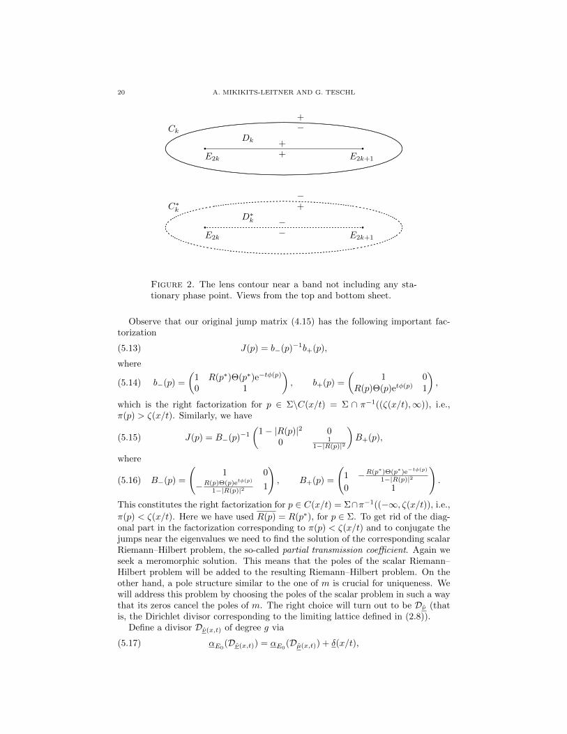
Figure 2. The lens contour near a band not including any sta-tionary phase point. Views from the top and bottom sheet.

Observe that our original jump matrix (4.15) has the following important fac-torization

(5.13) J(p) = b−(p)−1b+(p),

where

(5.14) b−(p) =

(1 R(p∗)Θ(p∗)e−tφ(p)

0 1

), b+(p) =

(1 0

R(p)Θ(p)etφ(p) 1

),

which is the right factorization for p ∈ Σ\C(x/t) = Σ ∩ π−1((ζ(x/t),∞)), i.e.,π(p) > ζ(x/t). Similarly, we have

(5.15) J(p) = B−(p)−1

(1− |R(p)|2 0

0 11−|R(p)|2

)B+(p),

where

(5.16) B−(p) =

(1 0

−R(p)Θ(p)etφ(p)

1−|R(p)|2 1

), B+(p) =

(1 −R(p∗)Θ(p∗)e−tφ(p)

1−|R(p)|2

0 1

).

This constitutes the right factorization for p ∈ C(x/t) = Σ∩π−1((−∞, ζ(x/t)), i.e.,

π(p) < ζ(x/t). Here we have used R(p) = R(p∗), for p ∈ Σ. To get rid of the diag-onal part in the factorization corresponding to π(p) < ζ(x/t) and to conjugate thejumps near the eigenvalues we need to find the solution of the corresponding scalarRiemann–Hilbert problem, the so-called partial transmission coefficient. Again weseek a meromorphic solution. This means that the poles of the scalar Riemann–Hilbert problem will be added to the resulting Riemann–Hilbert problem. On theother hand, a pole structure similar to the one of m is crucial for uniqueness. Wewill address this problem by choosing the poles of the scalar problem in such a waythat its zeros cancel the poles of m. The right choice will turn out to be Dν (thatis, the Dirichlet divisor corresponding to the limiting lattice defined in (2.8)).

Define a divisor Dν(x,t) of degree g via

(5.17) αE0(Dν(x,t)) = αE0

(Dµ(x,t)) + δ(x/t),


where

(5.18) δ`(x/t) = −2∑

ρk<ζ(x/t)

AE(ρk),`(ρk) +1

2πi

∫C(x/t)

log(1− |R|2)ζ`,

with C(x/t) = Σ ∩ π−1((−∞, ζ(x/t)) and ζ(x/t) as defined in (5.11).Then Dν(x,t) is nonspecial and π(νj(x, t)) = νj(x, t) ∈ R with precisely one in

each spectral gap (see [22]).We define the partial transmission coefficient as

(5.19)

T (p, x, t) =θ(z(p∞, x, t) + δ(x/t)

)θ(z(p∞, x, t)

) θ(z(p, x, t)

)θ(z(p, x, t) + δ(x/t)

) ··( ∏ρk<ζ(x/t)

exp(−∫ p

E0

ωρk ρ∗k

))exp

( 1

2πi

∫C(x/t)

log(1− |R|2)ωp p∞

),

where δ(x, t) is defined in (5.18) and ωp1 p2 is the Abelian differential of the thirdkind with poles at p1 and p2.

The function T (p, x, t) is meromorphic in Kg \ C(x/t) with first order poles atρk < ζ(x/t), νj(x, t) and first order zeros at µj(x, t).

Lemma 5.4. T (p, x, t) satisfies the following scalar meromorphic Riemann–Hilbertproblem:

(5.20)

T+(p, x, t) = T−(p, x, t)(1− |R(p)|2), p ∈ C(x/t),

(T (p, x, t)) =∑

ρk<ζ(x/t)

Dρ∗k −∑

ρk<ζ(x/t)

Dρk +Dµ(x,t) −Dν(x,t),

T (p∞, x, t) = 1.

Moreover,

(i)

T (p∗, x, t)T (p, x, t) =

g∏j=1

z − µj(x, t)z − νj(x, t)

, z = π(p).

(ii) T (p, x, t) = T (p, x, t) and in particular T (p, x, t) is real-valued for π(p) ∈R\σ(Hq).

Proof. The argument is similar to [22, Thm. 4.3]. The solution of a Riemann–Hilbert problem on the Riemann sphere is given by the Plemelj-Sokhotsky formula.Since our problem is now set on the Riemann surface Kg the Cauchy kernel is givenby the Abelian differential of the third kind ωp p∞ (cf. [35]). In particular, T (p, x, t)satisfies the jump condition from (5.20) along C(x/t). Next we have to check thatthe function T (p, x, t) extends to a single-valued function on Kg. For that purposenote that the only possible contribution which causes multi-valuedness may comefrom the b-cycles since all Abelian differentials are normalized to have vanishinga-periods. So for the b`-periods ` = 1, . . . , g we compute for p ∈ C(x/t)

limε↓0

T (p+ iε, x, t)

T (p− iε, x, t)= exp

(2πiδ`−

∫C(x/t)

log(1−|R|2)ζ`+∑

ρk<ζ(x/t)

4πiAE(ρk),`(ρk))),

which is indeed equals 1 by the choice of δ` in (5.18).


Concerning the poles and zeros of the function T (p, x, t) we see that by Riemann’svanishing theorem (cf. [34, Theorem A.13]) and the choice of the divisor Dν(x,t)

defined by (5.17) that the ratio of theta functions is meromorphic with simple zerosat µj and simple poles at νj . Moreover, from the product of the Blaschke factorswe get that T has simple poles at ρk and simple zeros at ρ∗k for which ρk < ζ(x/t)is valid.

To prove uniqueness let T be a second solution and consider T /T . Then T /Thas no jump and the Schwarz reflection principle implies that it extends to a mero-morphic function on Kg. Since the poles of T cancel the poles of T , its divisor

satisfies (T /T ) ≥ −Dµ(x,t). Since Dµ(x,t) is nonspecial, T /T has to be a constant

by the Riemann–Roch theorem (cf. [34, Theorem A.2]). Setting p = p∞, we see

that this constant is one, that is, T = T as claimed.Finally, T (p, x, t) = T (p, x, t) follows from uniqueness since both functions solve

(5.20).

We will also need the expansion around p∞ given by

Lemma 5.5. The asymptotic expansion of the partial transmission coefficient forp near p∞ is given by

(5.21) T (p, x, t) = 1± T1(x, t)√z

+O(1

z), p = (z,±),

where

(5.22)

T1(x, t) =−∑

ρk<ζ(x/t)

2

∫ ρk

E(ρk)

ωp∞,0 +1

2πi

∫C(x/t)

log(1− |R|2)ωp∞,0

− i∂y ln

(θ(z(p∞, y, t) + δ(x/t)

)θ(z(p∞, y, t)

) ) ∣∣∣∣∣y=x

,

and ωp∞,0 is the Abelian differential of the second kind defined in (3.15).

Proof. This can be verified similarly as in the case of the full transmission coefficient(cf. [29, Theorems 6.2 and 6.3] and by expanding the ratio of theta functions nearp∞.

Now that we have solved the scalar Riemann–Hilbert problem for T (p, x, t) wecan conjugate our original Riemann–Hilbert problem.

Since to each discrete eigenvalue there corresponds a soliton, it follows thatsolitons are represented in our Riemann–Hilbert problem by the pole conditions(4.32). For this reason we will study how poles can be dealt with in this section.We will follow closely the presentation of [24, Section 4].

In order to remove the poles there are two cases to distinguish. If ρj > ζ(x/t),the jump at ρj is exponentially close to the identity and there is nothing to do.

Otherwise, if ρj < ζ(x/t), we need to use conjugation to turn the jumps at thesepoles into exponentially decaying ones, following [11]. It turns out that we will haveto handle the poles at ρj and ρ∗j in one step in order to preserve symmetry and inorder to not add additional poles elsewhere.

Moreover, the conjugation of the Riemann–Hilbert problem also serves anotherpurpose, namely that the jump matrix can be separated into two matrices, onecontaining an off-diagonal term with exp(−tφ) and the other with exp(tφ). Withoutconjugation this is not possible for the jump on C(x/t) = Σ ∩ π−1

((−∞, ζ(x/t))

),


since in this case there also appears a diagonal matrix if one wants to separate thejump matrix.

For easy reference we note the following result, which can be verified by astraightforward calculation.

Lemma 5.6 (Conjugation). Assume that Σ ⊆ Σ. Let D be a matrix of the form

(5.23) D(p) =

(d(p∗) 0

0 d(p)

),

where d : Kg\Σ→ C is a sectionally analytic function. Set

(5.24) m(p) = m(p)D(p),

then the jump matrix transforms according to

(5.25) J(p) = D−(p)−1J(p)D+(p).

m(p) satisfies the symmetry condition (4.18) if and only if m(p) does. Further-more, m(p) satisfies the normalization condition (4.19) if m(p) satisfies (4.19) andd(p∞) = 1.

Lemma 5.7 ([26], Lem. 7.2). Introduce

(5.26) B(p, ρ) = Cρ(x, t)θ(z(p, x, t))

θ(z(p, x, t) + 2AE0(ρ))

B(p, ρ).

Then B(., ρ) is a well defined meromorphic function, with divisor

(5.27) (B(., ρ)) = −Dν +Dµ −Dρ∗ +Dρ,

where ν is defined via

(5.28) αE0(Dν) = αE0

(Dµ) + 2AE0(ρ).

Furthermore,

(5.29) B(p∞, ρ) = 1,

if

(5.30) Cρ(x, t) =θ(z(p∞, x, t) + 2AE0

(ρ))

θ(z(p∞, x, t)).

Now, we can show how to conjugate the jump corresponding to one eigenvaluefollowing [26].

Lemma 5.8. Assume that the Riemann–Hilbert problem for m has jump conditionsnear ρ and ρ∗ given by

(5.31)

m+(p) = m−(p)

(1 0γ(p)

π(p)−ρ 1

), p ∈ Σε(ρ),

m+(p) = m−(p)

(1 − γ(p∗)

π(p)−ρ0 1

), p ∈ Σε(ρ

∗),

and satisfies a divisor condition

(5.32) (m1) ≥ −Dµ∗ , (m2) ≥ −Dµ.


Then this Riemann–Hilbert problem is equivalent to a Riemann–Hilbert problem form which has jump conditions near ρ and ρ∗ given by

(5.33)

m+(p) = m−(p)

(1 B(p,ρ∗)(π(p)−ρ)

γ(p)B(p∗,ρ∗)

0 1

), p ∈ Σε(ρ),

m+(p) = m−(p)

(1 0

− B(p∗,ρ∗)(π(p)−ρ)γ(p∗)B(p,ρ∗)

1

), p ∈ Σε(ρ

∗),

divisor condition

(5.34) (m1) ≥ −Dν∗ , (m2) ≥ −Dν ,where Dν is defined via

(5.35) αE0(Dν) = αE0

(Dµ) + 2AE0(ρ),

and all remaining data conjugated (as in Lemma 5.6) by

(5.36) D(p) =

(B(p∗, ρ∗) 0

0 B(p, ρ∗)

).

Proof. Denote by U the interior of Σε(ρ). To turn γ into γ−1, introduce D by

D(p) =

(1 π(p)−ρ

γ(p)

− γ(p)π(p)−ρ 0

)(B(p∗, ρ∗) 0

0 B(p, ρ∗)

), p ∈ U,(

0 − γ(p∗)π(p)−ρ

π(p)−ργ(p∗) 1

)(B(p∗, ρ∗) 0

0 B(p, ρ∗)

), p∗ ∈ U,(

B(p∗, ρ∗) 0

0 B(p, ρ∗)

), else,

and note that D(p) is meromorphic away from the two circles. Now set m(p) =m(p)D(p). The claim about the divisors follows from noting, where the poles of

B(p, ρ) are.

Note that Lemma 5.8 can be applied iteratively to conjugate the eigenvaluesρj < ζ(x/t): start with the poles µ = µ0 and apply the lemma setting ρ = ρ1. Thisresults in new poles µ1 = ν. Then repeat this with µ = µ1, ρ = ρ2, and so on.

All in all we will now make the following conjugation step: abbreviate

γk(p, x, t) =−2R

1/22g+1(ρk)∏g

l=1(ρk − µl)ψq(p, x, t)

ψq(p∗, x, t)γk

and introduce

(5.37) D(p) =

(1 π(p)−ρk

γk(p,x,t)

−γk(p,x,t)π(p)−ρk 0

)D0(p), |π(p)−ρk|<ε

p∈Π+, ρk < ζ(x/t),(

0 −γk(p∗,x,t)π(p)−ρk

π(p)−ρkγk(p∗,x,t) 1

)D0(p), |π(p)−ρk|<ε

p∈Π−, ρk < ζ(x/t),

D0(p), else,

where

D0(p) =

(T (p∗, x, t) 0

0 T (p, x, t)

).


Note that D(p) is meromorphic in Kg\C(x/t) and that we have

(5.38) D(p∗) =

(0 11 0

)D(p)

(0 11 0

).

Now we conjugate our problem using D(p):

Theorem 5.9 (Conjugation). The function m2(p) = m(p)D(p), where D(p) isdefined in (5.37), is meromorphic away from C(x/t) and satisfies:

(i) The jump condition

(5.39) m2+(p) = m2

−(p)J2(p), p ∈ Σ,

where the jump matrix is given by

(5.40) J2(p) = D0−(p)−1J(p)D0+(p),

(ii) the divisor conditions

(5.41) (m21) ≥ −Dν(x,t)∗ , (m2

2) ≥ −Dν(x,t),

All jumps corresponding to poles, except for possibly one if ρk = ζ(x/t),are exponentially decreasing. In that case we will keep the pole conditionwhich is now of the form:

(5.42)

(m2

1(p) +γk(p, x, t)

π(p)− ρkT (p∗, x, t)

T (p, x, t)m2

2(p))≥ −Dν(x,t)∗ , near ρk,(γk(p∗, x, t)

π(p)− ρkT (p, x, t)

T (p∗, x, t)m2

1(p) +m22(p)

)≥ −Dν(x,t), near ρ∗k.

(iii) the symmetry condition

m2(p∗) = m2(p)

(0 11 0

),

(iv) and the normalization

m2(p∞) =(1 1

).

Proof. Invoking Lemma 5.6 and (4.15) we see that the jump matrix J2(p) is indeedgiven by (5.40). The divisor conditions follow from the one for T (p, x, t) and m(p).Moreover, using Lemma 5.8 one easily sees that the jump corresponding to ρk <ζ(x/t) (if any) is given by

(5.43)

J2(p) =

(1 T (p,x,t)(π(p)−ρk)

γk(p,x,t)T (p∗,x,t)

0 1

), p ∈ Σε(ρk),

J2(p) =

(1 0

−T (p∗,x,t)(π(p)−ρk)γk(p∗,x,t)T (p,x,t) 1

), p ∈ Σε(ρ

∗k),

and by Lemma 5.6 the jump corresponding to ρk > ζ(x/t) (if any) reads

(5.44)

J2(p) =

(1 0

γk(p,x,t)T (p∗,x,t)T (p,x,t)(π(p)−ρk) 1

), p ∈ Σε(ρk),

J2(p) =

(1 − γk(p∗,x,t)T (p,x,t)

T (p∗,x,t)(π(p)−ρk)

0 1

), p ∈ Σε(ρ

∗k).


That is, all jumps corresponding to the poles ρk 6= ζ(x/t) are exponentially decreas-ing. That the pole conditions are of the form (5.42) in the case ρk = ζ(x/t) canbe checked directly: just use the pole conditions of the original Riemann–Hilbertproblem (4.17) and the divisor condition (5.20) for T (p, x, t). Furthermore, by(4.18) and (5.38) one checks that the symmetry condition for m2 is fulfilled. FromT (p∞, x, t) = 1 we finally deduce

(5.45) m2(p∞) = m(p∞) =(1 1

),

which finishes the proof.

For p ∈ Σ\C(x/t) = Σ∩π−1((ζ(x/t),∞)

)the jump matrix J2 can be factorized

asJ2 = (b−)−1b+,

where b± = D−10 b±D0, that is,

(5.46)

b− =

(1 T (p,x,t)

T (p∗,x,t)R(p∗)Θ(p∗)e−tφ(p)

0 1

), b+ =

(1 0

T (p∗,x,t)T (p,x,t) R(p)Θ(p)etφ(p) 1

).

For p ∈ C(x/t) = Σ ∩ π−1((−∞, ζ(x/t))

)we can factorize J2 in the following way

J2 = (B−)−1B+,

where B± = D−1± B±D±, that is,

(5.47)

B− =

(1 0

−T−(p∗,x,t)T−(p,x,t)

R(p)Θ(p)1−|R(p)|2 et φ(p) 1

), B+ =

(1 − T+(p,x,t)

T+(p∗,x,t)R(p∗)Θ(p∗)1−|R(p)|2 e−t φ(p)

0 1

).

Note that by T (p, x, t) = T (p, x, t) we have

(5.48)T−(p∗, x, t)

T+(p, x, t)=T−(p∗, x, t)

T−(p, x, t)

1

1− |R(p)|2=T+(p, x, t)

T+(p, x, t), p ∈ C(x/t),

respectively

(5.49)T+(p, x, t)

T−(p∗, x, t)=

T+(p, x, t)

T+(p∗, x, t)

1

1− |R(p)|2=T−(p∗, x, t)

T−(p∗, x, t), p ∈ C(x/t).

We are now able to redefine the Riemann–Hilbert problem for m2(p) in such away that the jumps of the new Riemann–Hilbert problem will lie in the regionswhere they are exponentially close to the identity for large times. The followingtheorem can be checked by straightforward calculations:

Theorem 5.10 (Deformation). Define m3(p) by

(5.50) m3(p) =

m2(p)B+(p)−1, p ∈ Dk ∪Dj1, k < j,

m2(p)B−(p)−1, p ∈ D∗k ∪D∗j1, k < j,

m2(p)b+(p)−1, p ∈ Dk ∪Dj2, k > j,

m2(p)b−(p)−1, p ∈ D∗k ∪D∗j2, k > j,

m2(p), else,

where the matrices b± and B± are defined in (5.46) and (5.47), respectively. Herewe assume that the deformed contour is sufficiently close to the original one. Thenthe function m3(p) satisfies:


(i) The jump condition

(5.51) m3+(p) = m3

−(p)J3(p), for p ∈ Σ,

where the jump matrix J3 is given by

(5.52) J3(p) =

B+(p), p ∈ Ck ∪ Cj1, k < j,

B−(p)−1, p ∈ C∗k ∪ C∗j1, k < j,

b+(p), p ∈ Ck ∪ Cj2, k > j,

b−(p)−1, p ∈ C∗k ∪ C∗j2, k > j,

J2(p), else,

(ii) the divisor conditions

(5.53) (m31) ≥ −Dν(x,t)∗ , (m3

2) ≥ −Dν(x,t),

The jumps on the small circles around the eigenvalues remain unchanged.(iii) The symmetry condition

(5.54) m3(p∗) = m3(p)

(0 11 0

),

(iv) and the normalization

(5.55) m3(p∞) =(1 1

).

Here we have assumed that the reflection coefficient R(p) appearing in the jumpmatrices admits an analytic extension to the corresponding regions. Of course thisis not true in general, but we can always evade this obstacle by approximating R(p)by analytic functions. We relegate the details to Section 7.

The crucial observation now is that the jumps J3 on the oriented paths Ck, C∗kare of the form I + exponentially small asymptotically as t → ∞, at least awayfrom the stationary phase points zj , z

∗j . We thus hope we can simply replace these

jumps by the identity matrix (asymptotically as t→∞) implying that the solutionshould asymptotically be given by the constant vector

(1 1

). That this can in fact

be done will be shown in the next section by explicitly computing the contributionof the stationary phase points thereby showing that they are of the order O(t−1/2),that is,

m3(p) =(1 1

)+O(t−1/2)

uniformly for p away from the jump contour. Hence all which remains to obtainthe leading term Vl in Theorem 2.2 is to trace back the definitions of m3 and m2

and comparing with (4.13). First of all, since m3 and m2 coincide near p∞ we have

m2(p) =(1 1

)+O(t−1/2)

uniformly for p in a neighborhood of p∞. Consequently, by the definition of m2

(see Theorem 5.9), we have

m(p) =(T (p∗, x, t)−1 T (p, x, t)−1

)+O(t−1/2)

again uniformly for p in a neighborhood of p∞. Finally, using the expansion ofT (p, x, t) near p∞ (see Lemma 5.5) and then comparing the last identity with (4.13)shows

(5.56)

∫ ∞x

(V − Vq)(y, t)dy = 2iT1(x, t) +O(t−1/2),


where T1 is defined via (5.22), that is,

T1(x, t) =−∑

ρk<ζ(x/t)

2

∫ ρk

E(ρk)

ωp∞,0 +1

2πi

∫C(x/t)

log(1− |R|2)ωp∞,0

− i∂x ln

(θ(z(p∞, x, t) + δ(x/t)

)θ(z(p∞, x, t)

) ).

Similarly one obtains

(5.57) (V − Vq)(x, t) = O(t−1/2),

by using (4.27) instead of (4.13).Hence we have proven the leading term in Theorem 2.2, the next term will be

computed in Section 6.

Case (ii): The soliton region. In the case where no stationary phase points liein the spectrum the situation is similar to the case (i). In fact, it is much simplersince there is no contribution from the stationary phase points: There is a gap (thej-th gap, say) in which two stationary phase points exist. Similarly as in case (i)an investigation of the sign of Re(φ) shows the following:

Re(φ(p)) > 0, p ∈ Dk, k < j,

Re(φ(p)) < 0, p ∈ Dk, k > j.

Now we construct “lens-type” contours Ck (as shown in Figure 2) around everysingle band lying to the left of the j-th gap and make use of the factorizationJ2 = (b−)−1b+, where the matrices b− and b+ are defined in (5.46). We alsoconstruct such “lens-type” contours Ck around every single band lying to the rightof the j-th gap and make use of the factorization J2 = (B−)−1B+ with the matrices

B− and B+ given by (5.47). Indeed, in place of (5.50) we set

(5.58) m3(p) =

m2(p)B−1+ (p), p ∈ Dk, k < j,

m2(p)B−1− (p), p ∈ D∗k, k < j,

m2(p)b−1+ (p), p ∈ Dk, k > j,

m2(p)b−1− (p), p ∈ D∗k, k > j,

m2(p), else.

Now we are ready to prove Theorem 2.1 by applying Theorem A.8 in the followingway:

If |ζ(x/t) − ρk| > ε for all k we can choose γt0 = 0 and wt0 by removing alljumps corresponding to poles from wt. The error between the solutions of wt andwt0 is exponentially small in the sense of Theorem A.8, that is, ‖wt − wt0‖∞ ≤O(t−l) for any l ≥ 1. We have the one soliton solution (cf. Lemma 4.6) m0(p) =(f(p∗, x, t) f(p, x, t)

), where f(p) = 1 for p large enough. Using Lemma 5.5 we

compute

m(p) =m0(p)

(T (p∗, x, t)−1 0

0 T (p, x, t)−1

)=(

1 + T1(x,t)√z

+O(z−1) 1− T1(x,t)√z

+O(z−1)).


Comparing this expression with (4.13) yields∫ ∞x

(V − Vq)(y, t)dy = 2iT1(x, t) +O(t−n),

and thus by our definition of the limiting solution we finally have∫ ∞x

(V − Vl)(y, t)dy =

∫ ∞x

((V − Vq)(y, t)− (Vl − Vq)(y, t)

)dy = O(t−n),

for any n ≥ 1 if R(p) has an analytic extension. This proves the second part of thetheorem.

If |ζ(x/t) − ρk| < ε for some k, we choose γt0 = γk and wt0 ≡ 0. Again weconclude that the error between the solutions of wt and wt0 is exponentially small,that is, ‖wt−wt0‖∞ ≤ O(t−l), for any l ≥ 1. By Lemma 4.6 we have the one soliton

solution m0(p) =(f(p∗, x, t) f(p, x, t)

), with

f(p, x, t) = 1 +γk

z − ρkψl,ck(ρk, x, t)W(x,t)(ψl,ck(ρk, x, t), ψl,ck(p, x, t))

ψl,ck(p, x, t)cl,k(x, t),

for p large enough, where γk is defined as in (2.13). We will again use

m(p) = m0(p)

(T (p∗, x, t)−1 0

0 T (p, x, t)−1

)=(f(p∗,x,t)T (p∗,x,t)

f(p,x,t)T (p,x,t)

),

and now expand f(p) as in the proof of Lemma 4.6. Finally a comparison with(4.13) yields∫ ∞

x

(V − Vq)(y, t)dy = 2iT1(x, t) + 2γkψl,ck(ρk, x, t)

2

cl,k(x, t)+O(t−n),

and hence by our definition of the limiting solution (2.8) we obtain (2.10) for anyn ≥ 1 if R(p) has an analytic extension. Similarly we obtain (2.11) by using (4.27)instead of (4.13).

Case (iii): The transitional region. In the special case where the two stationaryphase points coincide (so zj = z∗j = Ek for some k) the Riemann–Hilbert problemarising above is of a different nature. We expect a similar behavior as in the constantbackground case [10] (cf. also the discussion in [22]). However, we will not treatthis case here.

6. The “local” Riemann–Hilbert problems on the small crosses

In the previous section we have reduced everything to the solution of the Riemann–Hilbert problem

m3+(p) = m3

−(p)J3(p),

(m31) ≥ −Dν(x,t)∗ , (m3

2) ≥ −Dν(x,t),

m3(p∗) = m3(p)

(0 11 0

)m3(p∞) =

(1 1

),

where the jump matrix J3 is given by (5.52). We have performed a deformation insuch a way that the jumps J3 on the oriented paths Ck, C∗k for k 6= j are of theform “I + exponentially small” asymptotically as t→∞. The same is true for theoriented paths Cj1, Cj2, C∗j1, C∗j2 at least away from the stationary phase points


Cj1 Cj2

C∗j1 C∗j2

qzjqE2j

qE2j+1

.

..............................................

..............................................

..............................................

..............................................

..............................................

.................. .

..............................................

..............................................

..............................................

..............................................

..............................................

..................

....................

..................

.................

...............

..................................

.....................................................................................

.................

...............

.................

..................

........

........

...

..................................................................................................................................

..... ..... ..... ..... ..... ..... ..... ..... ..... ..... ..... ..... ..... ..... ..... ..... ..... ..... ..... ..... ..... ..... ..... ..... ..... .....

............................................................................................

.........................................

C∗j1 C∗j2

Cj1 Cj2

qz∗jqE2j

qE2j+1

.

..............................................

..............................................

..............................................

..............................................

..............................................

...................

..............................................

..............................................

..............................................

..............................................

..............................................

.................. ....................

..................

.................

...............

.................

.................

.....................................................................................

.................

...............

.................

..................

....................... .... .... .... .... .... .... .... .... .... .... .... .... .... .... .... .... .... .... .... .... .... .... .... .... .... .... .... .... .... .... .... .... .... .... .... .... .... .... .... .... .... .... .... .... .... .... .... .... .... .... .... .... .... .... .........

...............................

..........................

.......................................................................

..................................................................................................................................

..... ..... ..... ..... ..... ..... ..... ..... ..... ..... ..... ..... ..... ..... ..... ..... ..... ..... ..... ..... ..... ..... ..... ..... ..... .....

Figure 3. The small cross containing the stationary phase pointzj and its flipping image containing z∗j . Views from the top andbottom sheet. Dotted curves lie in the bottom sheet.

zj , z∗j . The purpose of this section will be to derive the actual asymptotic rate at

which m3(p)→(1 1

)following again [22]. The jump contour near the stationary

phase points (cf. Figure 3) will be denoted by ΣC(zj) and ΣC(z∗j ). On these crossesthe jumps read

(6.1)

J3 = B+ =

(1 − T

T∗R∗Θ∗

1−R∗Re−t φ

0 1

), p ∈ Cj1,

J3 = B−1− =

(1 0

T∗

TRΘ

1−R∗Ret φ 1

), p ∈ C∗j1,

J3 = b+ =

(1 0

T∗

T RΘet φ 1

), p ∈ Cj2,

J3 = b−1− =

(1 − T

T∗R∗Θ∗e−t φ

0 1

), p ∈ C∗j2.

To reduce our Riemann–Hilbert problem to the one corresponding to the twocrosses we proceed as follows: We take a small disc D around zj(x/t) and project itto the complex plane using the canonical projection π. Now consider the (holomor-phic) Riemann–Hilbert problem in the complex plane with the very jump obtainedby projection and normalize it to be I near ∞.

The corresponding Riemann–Hilbert problem is solved in [25, Appendix A]. Toapply [25, Theorem A.1] we need the behavior of the jump matrix J3, that is, thebehavior of T (p, x, t) near the stationary phase points zj and z∗j .

The following lemma gives more information on the singularities of T (p, x, t) nearthe stationary phase points zj , j = 0, . . . , g and the band edges Ej , j = 0, . . . , 2g+1(setting E2g+1 =∞).

Lemma 6.1. For p near a stationary phase point zj or z∗j (not equal to a bandedge) we have

(6.2) T (p, x, t) = (z − zj)±iνe±(z), p = (z,±),


where e±(z) has continuous limits near zj and

(6.3) ν = − 1

2πlog(1− |R(zj)|2) > 0.

Here (z − zj)±iν = exp(±iν log(z − zj)), where the branch cut of the logarithm isalong the negative real axis.

For p near a band edge Ek ∈ C(x/t) we have

(6.4) T (p, x, t) = T±1(z)e±(z), p = (z,±),

where e±(z) is holomorphic near Ek if none of the νj is equal to Ek and e±(z) hasa first order pole at Ek = νj else.

Proof. By factorizing the jump according to 1− |R(p)|2 = (1− |R(zj)|2) 1−|R(p)|21−|R(zj)|2

one can rewrite (5.19). Then one considers the Abelian differential ωp p∗ for p ∈Kg\p∞ which is explicitly given by the formula (3.21). One has

(6.5)1

2

∫C(x/t)

ωp p∗ = ± log(z − zj)± α(zj) +O(z − zj), p = (z,±)

and thus

(6.6)

∫C(x/t)

ωp p∞ = ± log(z − zj)± α(zj) +O(z − zj), p = (z,±),

since∫C(x/t)

fωp p∞ = 12

∫C(x/t)

fωp p∗ for any symmetric function f(q) = f(q∗).

From this the first claim follows. For the second claim note that the function

t(p) =

T (z), p = (z,+) ∈ Π+,T (z)−1, p = (z,−) ∈ Π−,

satisfies the following (holomorphic) Riemann–Hilbert problem

t+(p) = t−(p)(1− |R(p)|2), p ∈ Σ,

t(p∞) = 1.

Thus T (p, x, t)/t(p) has no jump along C(x/t) and is therefore holomorphic nearC(x/t) away from band edges Ek = νj (where there is a simple pole) by the Schwarzreflection principle.

Moreover,

Lemma 6.2. We have

(6.7) e±(z) = e∓(z), p = (z,±) ∈ Σ \ C(x/t)

and(6.8)

e+(zj) = exp(iνα(zj)

)θ(z(p∞, x, t) + δ(x/t))

θ(z(p∞, x, t)

) θ(z(zj , x, t)

)θ(z(zj , x, t) + δ(x/t)

) ·· exp

(−

∑ρk<ζ(x/t)

∫ ρk

E(ρk)

ωzj z∗j +1

4πi

∫C(x/t)

log( 1− |R|2

1− |R(zj)|2)ωzj z∗j

),

where

(6.9) α(zj) = limp→zj

(1

2

∫C(x/t)

ωp p∗ − log(π(p)− zj

)).

Here α(zj) ∈ R and ωp p∗ is real on C(x/t).


Proof. The first claim follows from the fact that

T (p∗, x, t) = T (p, x, t) = T (p, x, t) for p ∈ Σ \ C(x/t).

For the second claim just follow the argument used in the proof of the previouslemma.

By Lemma 6.1 one deduces that near the stationary phase points the jumps aregiven by

(6.10)

B+ =

1 −(√

φ′′(zj)i (z − zj)

)2iνr

1−|r|2 e−t φ

0 1

, p ∈ Lj1,

B−1− =

1 0(√φ′′(zj)

i (z − zj))−2iν

r1−|r|2 et φ 1

, p ∈ L∗j1,

b+ =

1 0(√φ′′(zj)

i (z − zj))−2iν

ret φ 1

, p ∈ Lj2,

b−1− =

1 −(√

φ′′(zj)i (z − zj)

)2iν

re−t φ

0 1

, p ∈ L∗j2,

where (cf. eq. (6.2))

(6.11) r = R(zj)Θ(zj , x, t)e+(zj)

e+(zj)

(φ′′(zj)i

)iν

.

The error terms will satisfy appropriate Holder estimates, that is

(6.12) ‖B+(p)− B+(p)‖ ≤ C|z − zj |α, p = (z,+) ∈ Cj1,for any α < 1 and similarly for the other matrices. Thus the assumptions of [25,Theorem A.1] are satisfied and we can conclude that the solution on π

(ΣC(zj)

)is

of the form

(6.13) M(z) = I +M0

z − zj1

t1/2+O(t−α),

where

M0 = i√

i/φ′′(zj)

(0 −β(t)

β(t) 0

),(6.14)

β(t) =√νei(π/4−arg(r)+arg(Γ(iν)))e−tφ(zj)t−iν ,(6.15)

and 1/2 < α < 1. Now we lift this solution in the complex plane back to the smalldisc D on the Riemann surface Kg by setting

(6.16) M(p) =

M(z), p ∈ D,(0 11 0

)M(z)

(0 11 0

), p ∈ D∗.

Thus we conclude that the solution on ΣC(zj) is given by

(6.17) MC(p) = I +1

t1/2M0

z − zj+O(t−α), p = (z,+),


and the one on ΣC(z∗j ) reads

(6.18) MC(p) = I +1

t1/2M0

z − zj+O(t−α), p = (z,−).

Then

(6.19) m4(p) =

m3(p)MC(p)−1, p ∈ D,m3(p)MC(p)−1, p ∈ D∗,m3(p), else,

has no jump inside D ∪ D∗ but jumps on the boundary ∂D ∪ ∂D∗. All jumpsoutside D∪D∗ are of the form I+ exponentially small and the jump on ∂D∪∂D∗is of the form I + O(t−1/2). In order to identify the leading behavior it remainsto rewrite the Riemann–Hilbert problem for m4 as a singular integral equationfollowing Section A. Let the operator Cw4 : L2(Σ4)→ L2(Σ4) be defined by

(6.20) Cw4f = C−(fw4)

for a vector valued f , where w4 = J4 − I and

(6.21) (C±f)(q) = limp→q∈Σ4

1

2πi

∫Σ4

f Ωνp , Ωνp =

(Ων∗,p∞p 0

0 Ων,p∞p

),

are the Cauchy operators for our Riemann surface. In particular, Ων,qp is the Cauchy

kernel given by

(6.22) Ων,qp = ωp q +

g∑j=1

Iν,qj (p)ζj ,

where

(6.23) Iν,qj (p) =

g∑`=1

cj`(ν)

∫ p

q

ων`,0.

Here ωq,0 is the (normalized) Abelian differential of the second kind with a secondorder pole at q (cf. Remark 6.4 below) and ωp q denotes the Abelian differential of

the third kind with simple poles at p and q. Note that Iν,qj (p) has first order poles

at the points ν.

The constants cj`(ν) are chosen such that Ων,qp is single valued, that is,

(6.24) (c`k(ν))1≤`,k≤g =

g∑j=1

ck(j)µj−1` dπ

R1/22g+2(µ`)

−1

1≤`,k≤g

where ck(j) are defined in (3.6) (cf. Lemma A.3).Consider the solution µ4 of the singular integral equation

(6.25) µ =(1 1

)+ Cw4µ in L2(Σ4).

Then the solution of our Riemann–Hilbert problem is given by

(6.26) m4(p) =(1 1

)+

1

2πi

∫Σ4

µ4 w4 Ωνp .

By ‖w4‖∞ = O(t−1/2) Neumann’s formula implies

(6.27) µ4(q) = (I− Cw4)−1(1 1

)=(1 1

)+O(t−1/2).


Moreover,

(6.28) w4(p) =

− M0

z−zj1t1/2

+O(t−α), p ∈ ∂D,− M0

z−zj1t1/2

+O(t−α), p ∈ ∂D∗.

Hence we obtain

m4(p) =(1 1

)−(1 1

)M0

t1/21

2πi

∫∂D

1

π − zjΩνp

−(1 1

)M0

t1/21

2πi

∫∂D∗

1

π − zjΩνp +O(t−α)

=(1 1

)−(1 1

)M0

t1/2Ωνp(zj)−

(1 1

)M0

t1/2Ωνp(z∗j ) +O(t−α)

=(1 1

)−

√i

φ′′(zj)t×

×(

iβΩν∗,p∞p (zj)− iβΩ

ν∗,p∞p (z∗j ) −iβΩ

ν,p∞p (zj) + iβΩ

ν,p∞p (z∗j )

)+O(t−α).(6.29)

Since we need the asymptotic expansions around p∞ we note

Lemma 6.3. We have

(6.30) Ων,p∞p (zj) = Λν1(zj)ζ + Λ

ν2(zj)ζ

2 +O(ζ3)

for ζ = z−1/2 being the local chart near p∞ and

Λν1(zj) = ωp∞,0(zj)−

g∑k=1

g∑`=1

ck`(ν)αg−1(ν`)ζk(zj),(6.31)

Λν2(zj) = ωp∞,1(zj)−

1

2

g∑k=1

g∑`=1

ck`(ν)ζk(zj),(6.32)

where ωq,k, k = 0, 1, . . . , is an Abelian differential of the second kind with a singlepole of order k + 2 at q and αg−1(ν`) denotes a constant defined in Remark 6.4below.

Proof. Use the local coordinate ζ = z−1/2 near p∞ = (∞,∞) and expand thedifferential ωpp∞ like it is done in [35, Theorem 4.1] and

∫ pp∞

ων`,0 by using the

expression (6.33). For g ≥ 1 one gets

ων,0(ζ) = −αg−1(ν)− ζ +O(ζ2)

and thus the claimed formulas for Λν1(zj) and Λ

ν2(zj) follow.

Remark 6.4. The Abelian differential appearing in the previous lemma is explicitlygiven by

(6.33) ων,0 =

R1/22g+1 +R

1/22g+1(ν) +

R′2g+1(ν)

2R1/22g+1(ν)

(π − ν) + Pν,0 · (π − ν)2

2(π − ν)2R1/22g+1

dπ,


with Pν,0 a polynomial of degree g− 1 which has to be determined from the normal-ization. We will use the notation

(6.34) Pν,0(z) =

g−1∑j=0

αj(ν)zj .

Concerning the Abelian differential ωp∞,0 we refer to (3.15). The differential ωp∞,1is given by

(6.35) ωp∞,1 =(−R

1/22g+1

2+ Pp∞,1

) dπ

R1/22g+1

,

where Pp∞,1 is a polynomial of degree g − 1 which has to be determined by thevanishing aj-periods as usual.

Note that the following relations are valid

(6.36)ωp∞,0(z∗j ) = −ωp∞,0(zj),

ωp∞,1(z∗j ) + ωp∞,1(zj) = −1,

and

(6.37) ck`(ν∗) = −ck`(ν), ζk(z∗j ) = −ζk(zj).

Moreover, the coefficients αj(ν), j = 0, . . . , g − 1 of the polynomial Pν,0 fulfill therelation

(6.38) αj(ν∗) = −αj(ν), j = 0, . . . , g − 1.

Now we come to prove Theorem 2.2. As in the previous section, the asymptoticscan be read off by using

(6.39) m(p) = m4(p)

(1

T (p∗,x,t) 0

0 1T (p,x,t)

)for p near p∞ and comparing with (4.13). From that one deduces

m2(p) =m42(p)T (p)−1 =

=1 +(√ i

φ′′(zj)t

(iβΛ

ν1(zj)− iβΛ

ν1(z∗j )

)− T1(x, t) +O(t−α)

) 1√z

+O(z−1),

where we have used (6.29), (6.30) and (5.21). Comparing this asymptotic expansionwith (4.13) yields∫ +∞

x

(V − Vq)(y)dy = 2

√i

φ′′(zj)t

(βΛ

ν1(zj)− βΛ

ν1(z∗j )

)+ 2iT1(x, t) +O(t−α).

Invoking (6.36), (6.37) and (6.38) one gets

(6.40)Λν1(z∗j ) = −Λ

ν1(zj),

Λν∗

1 (zj) = Λν1(zj),

and therefore

(6.41)

∫ ∞x

(V −Vq)(y, t)dy = 4

√i

φ′′(zj)tRe(β(x, t)

)Λν1(x, t)+2iT1(x, t)+O(t−α).


Finally, using the definition of the limiting solution (2.8) proves the claim. Notethat one obtains the same result if one compares the expressions for the componentm1.

Similarly one obtains (2.17) by using (4.27) instead of (4.13).

7. Analytic Approximation

In this section we want to show how to get rid of the analyticity assumptionon the reflection coefficient R(p). To this end we will split R(p) into an analyticpart Ra,t plus a small rest Rr,t following the ideas of [8] (see also [25, Sect. 6]).The analytic part will be moved to regions of the Riemann surface while the restremains on Σ = π−1

(σ(Hq)

). This needs to be done in such a way that the rest is

of O(t−1) and the growth of the analytic part can be controlled by the decay of thephase.

In order to avoid problems when one of the poles νj hits Σ, we have to make theapproximation in such a way that the nonanalytic rest vanishes at the band edges.That is, split R according to

R(p) =R(E2j)(z − E2j)(E2j+1 − i)

(E2j+1 − E2j)(z − i)+R(E2j+1)

(z − E2j+1)(E2j − i)

(E2j − E2j+1)(z − i)

+Qj(p)R(p), p = (z,±),(7.1)

where Qj(p) is a rational function with first order zeros at E2j , E2j+1 and with all

other zeros and poles away from Σ, and approximate R. Note that if R ∈ Cl(Σ),

then R ∈ Cl−1(Σ).We will use different splittings for different bands depending on whether the

band contains our stationary phase point zj(x/t) or not. We will begin with somepreparatory lemmas.

For the bands containing no stationary phase points we will use a splitting basedon the following Fourier transform associated with the background operator Hq.Given R ∈ Cl(Σ) we can write

(7.2) R(p) =

∫RR(x)ψq(p, x, 0)dx,

where ψq(p, x, t) denotes the time-dependent Baker–Akhiezer function and (cf. [14],[12])

(7.3) R(x) =1

2πi

∮Σ

R(p)ψq(p, x, 0)i∏gj=1(π(p)− µj)

2R1/22g+1(p)

dπ(p).

If we make use of (3.14), the above expression for R(p) is of the form

(7.4) R(p) =

∫RR(x)θq(p, x, 0) exp

(ixk(p)

)dx.

where k(p) = −i∫ pE0ωp∞,0 and θq(p, n, t) collects the remaining parts in (3.14).

Using k(p) as a new coordinate and performing l integration by parts one obtains(cf. [12])

(7.5) |R(x)| ≤ const

1 + |x|l

provided R ∈ Cl(Σ).


Lemma 7.1. Suppose R ∈ L1(R), xlR(x) ∈ L1(R) and let β > 0 be given. Thenwe can split R(p) according to

R(p) = Ra,t(p) +Rr,t(p),

such that Ra,t(p) is analytic for in the region 0 < Im(k(p)) < ε and

|Ra,t(p)e−βt| = O(t−l), 0 < Im(k(p)) < ε,(7.6)

|Rr,t(p)| = O(t−l), p ∈ Σ.(7.7)

Proof. We choose

Ra,t(p) =

∫ ∞x=−K(t)

R(x)θq(p, x, 0) exp(ixk(p)

)dx

with K(t) = β0

ε t for some positive β0 < β. Then, for 0 < Im(k(p)) < ε,∣∣Ra,t(k)e−βt∣∣ ≤ Ce−βt

∫ ∞x=−K(t)

|R(x)|e−Im(k(p))xdx

≤ Ce−βteK(t)ε‖F‖1 = ‖R‖1e−(β−β0)t,

which proves the first claim. Similarly, for p ∈ Σ,

|Rr,t(k)| ≤ C∫ ∞x=K(t)

xl|R(−x)|xl

dx ≤ C ‖xlR(−x)‖1K(t)l

≤ C

tl

For the band which contains zj(x/t) we need to take the small vicinities of thestationary phase points into account. Since the phase is cubic near these points, wecannot use it to dominate the exponential growth of the analytic part away from Σ.Hence we will take the phase as a new variable and use the Fourier transform withrespect to this new variable. Since this change of coordinates is singular near thestationary phase points, there is a price we have to pay, namely, requiring additionalsmoothness for R(p).

Without loss of generality we will choose the path of integration in our phaseφ(p), defined in (4.21), such that φ(p) is continuous (and thus analytic) in Dj,1

with continuous limits on the boundary (cf. Figure 1). We begin with

Lemma 7.2. Suppose R(p) ∈ C5(Σ). Then we can split R(p) according to

(7.8) R(p) = R0(p) +z − zjz − i

H(p), p = (z,±) ∈ Σ ∩Dj,1,

where R0(p) is a real rational function on M such that H(p) vanishes at zj, z∗j of

order three and has a Fourier transform

(7.9) H(p) =

∫RH(x)exφ(p)dx,

with xH(x) integrable. Here φ denotes the phase defined in (4.21).

Proof. We begin by choosing a rational function R0(p) = a(z) + b(z)R1/22g+1(p) with

p = (z,±) such that a(z), b(z) are real-valued rational functions which are chosensuch that a(z) matches the values of Re(R(p)) and its first four derivatives at zj

and i−1b(z)R1/22g+1(p) matches the values of Im(R(p)) and its first four derivatives


at zj . Moreover, all poles are chosen away from Σ. Since R(p) is C5 we infer thatH(p) ∈ C4(Σ) and it vanishes together with its first three derivatives at zj , z

∗j .

Note that φ(p)/i, where φ is defined in (4.21) has a maximum at z∗j and a mini-mum at zj . Thus the phase φ(p)/i restricted to Σ∩Dj,1 gives a one to one coordinatetransform Σ∩Dj,1 → [φ(z∗j )/i, φ(zj)/i] and we can hence express H(p) in this newcoordinate (setting it equal to zero outside this interval). The coordinate transformlocally looks like a cube root near zj and z∗j , however, due to our assumption that

H vanishes there, H is still C2 in this new coordinate and the Fourier transformwith respect to this new coordinates exists and has the required properties.

Moreover, as in Lemma 7.1 we obtain:

Lemma 7.3. Let H(p) be as in the previous lemma. Then we can split H(p)according to H(p) = Ha,t(p) + Hr,t(p) such that Ha,t(p) is analytic in the regionRe(φ(p)) < 0 and

(7.10) |Ha,t(p)eφ(p)t/2| = O(1), p ∈ Dj,1, |Hr,t(p)| = O(t−1), p ∈ Σ.

Proof. We choose Ha,t(p) =∫∞x=−K(t)

H(x)exφ(p)dx with K(t) = t/2. Then we can

proceed as in Lemma 7.1:

|Ha,t(p)eφ(p)t/2| ≤ ‖H‖1|e−K(t)φ(p)+φ(p)t/2| ≤ ‖H‖1

and

|Hr,t(p)| ≤1

K(t)

∫ ∞x=K(t)

x|H(−x)|dx ≤ C

t.

Clearly an analogous splitting exists for p ∈ Σ ∩Dj2.Now we are ready for our analytic approximation step. First of all recall that our

jump is given in terms b± and B± defined in (5.14) and (5.16), respectively. While

b± are already in the correct form for our purpose, this is not true for B± sincethey contain the non-analytic expression |T (p)|2. To remedy this we will rewrite

B± in terms of the left rather than the right scattering data. For this purposelet us use the notation Rr(p) ≡ R+(p) for the right and Rl(p) ≡ R−(p) for theleft reflection coefficient. Moreover, let Tr(p, x, t) ≡ T (p, x, t) be the right andTl(p, x, t) ≡ T (p)/Tr(p, x, t) be the left partial transmission coefficient.

With this notation we have

(7.11) J2(p) =

b−(p)−1b+(p), π(p) > ζ(x/t),

B−(p)−1B+(p), π(p) < ζ(x/t),

where

b− =

(1 Tr(p,x,t)

Tr(p∗,x,t)Rr(p∗)Θ(p∗)e−tφ(p)

0 1

),

b+ =

(1 0

Tr(p∗,x,t)Tr(p,x,t) Rr(p)Θ(p)e−tφ(p) 1

),


and

B− =

(1 0

−Tr,−(p∗,x,t)Tr,−(p,x,t)

Rr(p)Θ(p)|T (p)|2 et φ(p) 1

),

B+ =

(1 − Tr,+(p,x,t)

Tr,+(p∗,x,t)Rr(p∗)Θ(p∗)|T (p)|2 e−t φ(p)

0 1

).

Using (4.8) we can write

B− =

(1 0

Tl(p∗,x,t)

Tl(p,x,t)Rl(p)Θ(p)e−tφ(p) 1

),

B+ =

(1 Tl(p,x,t)

Tl(p∗,x,t)Rl(p

∗)Θ(p∗)e−tφ(p)

0 1

).

Now we split Rr(p) = Ra,t(p)+Rr,t(p) by splitting Rr(p) defined via (7.1) accordingto Lemma 7.1 for π(p) ∈ [E2k, E2k+1] with k < j (i.e., not containing ζ(x/t))and according to Lemma 7.3 for π(p) ∈ [E2j , ζ(x/t)]. In the same way we splitRl(p) = Ra,t(p) + Rr,t(p) for π(p) ∈ [ζ(x/t), E2j+1] and π(p) ∈ [E2k, E2k+1] withk > j. For β in Lemma 7.1 we can choose

(7.12) β =

minp∈Ck −Re(φ(p)) > 0, π(p) > ζ(x/t),minp∈Ck Re(φ(p)) > 0, π(p) < ζ(x/t).

In this way we obtain

b±(p) = ba,t,±(p)br,t,±(p) = br,t,±(p)ba,t,±(p),

B±(p) = Ba,t,±(p)Br,t,±(p) = Br,t,±(p)Ba,t,±(p).

Here ba,t,±(p), br,t,±(p) (resp. Ba,t,±(p), Br,t,±(p)) denote the matrices obtained

from b±(p) (resp. B±(p)) by replacing Rr(p) (resp. Rl(p)) with Ra,t(p), Rr,t(p),respectively. Now we can move the analytic parts into regions of the Riemannsurface as in Section 5 while leaving the rest on Σ. Hence, rather than (5.52), thejump now reads

(7.13) J3(p) =

ba,t,+(p), p ∈ Ck, π(p) > ζ(x/t),

ba,t,−(p)−1, p ∈ C∗k , π(p) > ζ(x/t),

br,t,−(p)−1br,t,+(p), p ∈ π−1((ζ(x/t),+∞)),

Ba,t,+(p), p ∈ Ck, π(p) < ζ(x/t),

Ba,t,−(p)−1, p ∈ C∗k , π(p) < ζ(x/t),

Br,t,−(p)−1Br,t,+(p), p ∈ π−1(−∞, ζ(x/t))).

By construction Ra,t(p) = R0(p) + (π(p) − π(zj))Ha,t(p) will satisfy the requiredLipschitz estimate in a vicinity of the stationary phase points (uniformly in t) andthe jump will be J3(p) = I + O(t−1). The remaining parts of Σ can be handledanalogously and hence we can proceed as in Section 6.

Appendix A. Singular integral equations

In the complex plane, the solution of a Riemann–Hilbert problem can be reducedto the solution of a singular integral equation (see [3]). In our case the underlyingspace is a Riemann surface M. The purpose of this appendix is to generalize this


approach to meromorphic vector Riemann–Hilbert problem with simple poles at ρ,ρ∗ of the type

m+(p) = m−(p)J(p), p ∈ Σ,

(m1) ≥ −Dµ∗ −Dρ, (m2) ≥ −Dµ −Dρ∗ ,(m1(p)−

R1/22g+2(ρ)∏g

k=1(ρ− µk)

γjπ(p)− ρ

ψq(p)

ψq(p∗)m2(p)

)≥ −D∗µ, near ρ,(A.1)

(−

R1/22g+2(ρ)∏g

k=1(ρ− µk)

γ

π(p)− ρψq(p)

ψq(p∗)m1(p) +m2(p)

)≥ −Dµ, near ρ∗,

m(p∗) = m(p)

(0 11 0

),

m(p∞) =(1 1

),

Since we require the symmetry condition (4.18) for our Riemann–Hilbert problems,we need to adapt the usual Cauchy kernel to preserve this symmetry. Moreover,we keep the single soliton as an inhomogeneous term which will play the role of theleading asymptotics in our applications.

Concerning the jump contour Σ and the jump matrix J we will make the followingassumptions:

Hypothesis H. A.1. Let Σ consist of a finite number of smooth oriented finitecurves in M which intersect at most finitely many times with all intersections beingtransversal. Assume that the contour Σ does not contain any of the points µ andis invariant under p 7→ p∗. It is oriented such that under the mapping p 7→ p∗ se-quences converging from the positive sided to Σ are mapped to sequences convergingto the negative side. The divisor Dµ is nonspecial.

The jump matrix J is nonsingular and can be factorized according to J =b−1− b+ = (I − w−)−1(I + w+), where w± = ±(b± − I) are Holder continuous and

satisfy

(A.2) w±(p∗) = −(

0 11 0

)w∓(p)

(0 11 0

), p ∈ Σ.

Moreover,

(A.3) ‖w‖∞ = ‖w+‖L∞(Σ) + ‖w−‖L∞(Σ) <∞.

Remark A.2. The assumption that that none of the poles µ lie on our contour Σcan be made without loss of generality if the jump is analytic since we can move thecontour a little without changing the value at p∞ (which is the only value we areeventually interested in). Alternatively, the case where one (or more) of the polesµj lies on Σ can be included if one assumes that w± has a first order zero at µj.In fact, in this case one can replace µ(s) by µ(s) = (π(s) − µj)µ(s) and w±(s) byw±(s) = (π(s)− µj)−1w±(s).

Otherwise one could also assume that the matrices w± are Holder continuous and

vanish at such points. Then one can work with the weighted measure −iR1/22g+1(p)dπ

on Σ. In fact, one can show that the Cauchy operators are still bounded in thisweighted Hilbert space (cf. [19, Thm. 4.1]).


Our first step is to replace the classical Cauchy kernel by a ”generalized” Cauchykernel appropriate to our Riemann surface. In order to get a single valued kernelwe need again to admit g poles. We follow the construction from [30, Sec. 4]/

Lemma A.3 ([22, 25]). Let Dµ be nonspecial and introduce the differential

(A.4) Ωµ,ρp = ωp ρ +

g∑j=1

Iµ,ρ

j (p)ζj ,

where

(A.5) Iµ,ρ

j (p) =

g∑`=1

cj`(µ)

∫ p

ρ

ωµ`,0.

Here ωq,0 is the (normalized) Abelian differential of the second kind with a secondorder pole at q (cf. Remark 6.4) and the matrix cj` is defined as the inverse matrixof η`(µj), where ζ` = η`(z)dz is the chart expression in a local chart near µj (thesame chart used to define ωµj ,0).

Then Ωµ,ρp is single valued as a function of p with first order poles at the points

µ.

Next we show that the Cauchy kernel introduced in (A.4) has indeed the correctproperties. We will abbreviate Lp(Σ) = Lp(Σ,C2).

Theorem A.4 ([22, 25]). Set

(A.6) Ωµ,ρp =

(Ωµ∗,ρ∗

p 0

0 Ωµ,ρp

),

and define the matrix operators as follows. Given a 2 × 2 matrix f defined on Σwith Holder continuous entries, let

(A.7) (Cf)(p) =1

2πi

∫Σ

f(s)Ωµ,ρp , for p 6∈ Σ,

and

(A.8) (C±f)(q) = limp→q∈Σ

(Cf)(p)

from the left and right of Σ respectively (with respect to its orientation). Then

(i) The operators C± are given by the Plemelj formulas

(C+f)(q)− (C−f)(q) = f(q),

(C+f)(q) + (C−f)(q) =1

πi−∫

Σ

f Ωµ,ρq ,

and extend to bounded operators on L2(Σ). Here −∫

denotes the principalvalue integral, as usual, and the bound can be chosen independent of thedivisor as long as it stays some finite distance away from Σ.

(ii) Cf is a meromorphic function off Σ, with divisor given by ((Cf)j1) ≥−Dµ∗ and ((Cf)j2) ≥ −Dµ.

(iii) (Cf)(ρ∗) = (0 ∗), (Cf)(ρ) = (∗ 0).


Furthermore, C restricts to L2s(Σ), that is

(A.9) (Cf)(p∗) = (Cf)(p)

(0 11 0

), p ∈M\Σ

for f ∈ L2s(Σ) and if w± satisfy (A.2) we also have

(A.10) C±(fw∓)(p∗) = C∓(fw±)(p)

(0 11 0

), p ∈ Σ.

Now, let the operator Cw : L2s(Σ)→ L2

s(Σ) be defined by

(A.11) Cwf = C+(fw−) + C−(fw+), f ∈ L2s(Σ),

for a 2× 2 matrix valued f , where

w+ = b+ − I and w− = I− b−.Recall from Lemma 4.6 that the unique solution corresponding to J ≡ I is given by

m0(p) =(f(p∗) f(p)

),

for some given f(p) with (f) ≥ −Dµ−Dρ∗ . Since we assumed Dµ to be away from

Σ, we clearly have m0 ∈ L2s(Σ).

Theorem A.5 ([22, 25]). Assume Hypothesis A.1 and let m0 ∈ C2 be given.Suppose m solves the Riemann–Hilbert problem (A.1). Then

(A.12) m(p) = (1− c0)m0(p) +1

2πi

∫Σ

µ(s)(w+(s) + w−(s))Ωµ,ρp ,

where

µ = m+b−1+ = m−b

−1− and c0 =

(1

2πi

∫Σ

µ(s)(w+(s) + w−(s))Ωµ,ρp∞

)1

.

Here (m)j denotes the j’th component of a vector. Furthermore, µ solves

(A.13) (I− Cw)µ = (1− c0)m0(p).

Conversely, suppose µ solves

(A.14) (I− Cw)µ = m0,

and

c0 =

(1

2πi

∫Σ

µ(s)(w+(s) + w−(s))Ωµ,ρp∞

)1

6= 0,

then m defined via (A.12), with (1− c0) = (1− c0)−1 and µ = (1− c0)−1µ, solvesthe Riemann–Hilbert problem (A.1) and µ = m±b

−1± .

Hence we have a formula for the solution of our Riemann–Hilbert problem m(z)in terms of (I−Cw)−1m0 and this clearly raises the question of bounded invertibilityof I− Cw. This follows from Fredholm theory (cf. e.g. [38]):

Lemma A.6 ([22, 25]). Assume Hypothesis A.1. Then the operator I − Cw isFredholm of index zero,

(A.15) ind(I− Cw) = 0.

By the Fredholm alternative, it follows that to show the bounded invertibility ofI− Cw we only need to show that ker(I− Cw) = 0. The latter being equivalent tounique solvability of the corresponding vanishing Riemann–Hilbert problem.


Corollary A.7. Assume Hypothesis A.1.A unique solution of the Riemann–Hilbert problem (A.1) exists if and only if the

corresponding vanishing Riemann–Hilbert problem, where the normalization condi-tion is given by m(p∞) =

(0 0

), has at most one solution.

We are interested in comparing two Riemann–Hilbert problems associated withrespective jumps w0 and w with ‖w − w0‖∞ small, where

(A.16) ‖w‖∞ = ‖w+‖L∞(Σ) + ‖w−‖L∞(Σ).

For such a situation we have the following result:

Theorem A.8 ([24]). Assume that for some data wt0 the operator

(A.17) I− Cwt0 : L2(Σ)→ L2(Σ)

has a bounded inverse, where the bound is independent of t.Furthermore, assume wt satisfies

(A.18) ‖wt − wt0‖∞ ≤ α(t)

for some function α(t) → 0 as t → ∞. Then (I − Cwt)−1 : L2(Σ) → L2(Σ) alsoexists for sufficiently large t and the associated solutions of the Riemann–Hilbertproblems (A.1) only differ by O(α(t)).

Acknowledgments. We want to thank Ira Egorova for most helpful discussionson this topic and pointing out several misprints in the original version of this man-uscript.

References

[1] M. J. Ablowitz and A. C. Newell, The decay of the continuous spectrum for solutions of

the Korteweg–de Vries equation, J. Math. Phys. 14, 1277–1284 (1973).

[2] M. J. Ablowitz and H. Segur, Asymptotic solutions of the Korteweg–de Vries equation,Stud. Appl. Math 57, 13–44 (1977).

[3] R. Beals and R. Coifman, Scattering and inverse scattering for first order systems,

Comm. in Pure and Applied Math. 37, 39–90 (1984).[4] A. Boutet de Monvel, I. Egorova, and G. Teschl, Inverse scattering theory for one-

dimensional Schrodinger operators with steplike finite-gap potentials, J. d’Analyse Math.

106:1, 271–316, (2008).[5] A. M. Budylin and V. S. Buslaev, Quasiclassical integral equations and the asymptotic

behavior of solutions of the Korteweg–de Vries equation for large time values, Dokl.

Akad. Nauk 348:4, 455–458 (1996). (Russian)[6] V. S. Buslaev, Use of the determinant representation of solutions of the Korteweg–de

Vries equation for the investigation of their asymptotic behavior for large times, UspekhiMat. Nauk 36:4, 217–218 (1981). (Russian)

[7] V. S. Buslaev and V. V. Sukhanov, Asymptotic behavior of solutions of the Korteweg–de

Vries equation, Jour. Sov. Math. 34, 1905–1920 (1986).[8] P. Deift, X. Zhou, A steepest descent method for oscillatory Riemann–Hilbert problems,

Ann. of Math. (2) 137, 295–368 (1993).[9] P. A. Deift, A. R. Its, and X. Zhou, Long-time asymptotics for integrable nonlinear

wave equations, in “Important developments in soliton theory”, 181–204, Springer Ser.Nonlinear Dynam., Springer, Berlin, 1993.

[10] P. Deift, S. Venakides, and X. Zhou, The collisionless shock region for the long timebehavior of solutions of the KdV equation, Comm. in Pure and Applied Math. 47, 199–206 (1994).

[11] P. Deift, S. Kamvissis, T. Kriecherbauer, and X. Zhou, The Toda rarefaction problem,Comm. Pure Appl. Math. 49, no. 1, 35–83 (1996).


[12] I. Egorova and G. Teschl, On the Cauchy problem for the Korteweg–de Vries equation

with steplike finite-gap initial data II. Perturbations with finite moments, J. d’Analyse

Math. (to appear).[13] I. Egorova and G. Teschl, A Paley-Wiener theorem for periodic scattering with applica-

tions to the Korteweg-de Vries equation, Zh. Mat. Fiz. Anal. Geom. 6:1, 21–33 (2010).

[14] I. Egorova, K. Grunert, and G. Teschl, On the Cauchy problem for the Korteweg–de Vriesequation with steplike finite-gap initial data I. Schwartz-type perturbations, Nonlinearity

22, 1431–1457 (2009).

[15] H. Farkas and I. Kra, Riemann Surfaces, 2nd edition, GTM 71, Springer, New York,1992.

[16] F. Gesztesy and H. Holden, Soliton Equations and Their Algebro-Geometric Solutions;

Volume I: (1+1)-Dimensional Continuous Models, Cambridge Studies in AdvancedMathematics 79, Cambridge University Press, Cambridge, 2003.

[17] C. S. Gardner, J. M. Green, M. D. Kruskal, and R. M. Miura, A method for solving theKorteweg–de Vries equation, Phys. Rev. Letters 19, 1095–1097 (1967).

[18] A. R. Its, Asymptotic behavior of the solutions to the nonlinear Schrodinger equation,

and isomonodromic deformations of systems of linear differential equations, Soviet.Math. Dokl. 24:3, 452–456 (1981).

[19] I. Gohberg and N. Krupnik, One-Dimensional Linear Singular Integral Equations,

Birkhauser, Basel, 1992.[20] K. Grunert and G. Teschl, Long-time asymptotics for the Korteweg–de Vries Equation

via nonlinear steepest descent, Math. Phys. Anal. Geom. 12, 287–324 (2009).

[21] S. Kamvissis and G. Teschl, Stability of periodic soliton equations under short rangeperturbations, Phys. Lett. A, 364-6, 480–483 (2007).

[22] S. Kamvissis and G. Teschl, Stability of the periodic Toda lattice under short range

perturbations, arXiv:0705.0346.[23] E.A. Kuznetsov and A.V. Mikhaılov, Stability of stationary waves in nonlinear weakly

dispersive media, Soviet Phys. JETP 40, no. 5, 855–859 (1975).[24] H. Kruger and G. Teschl, Long-time asymptotics for the Toda lattice in the soliton region,

Math. Z. 262, 585–602 (2009).

[25] H. Kruger and G. Teschl, Long-time asymptotics of the Toda lattice for decaying initialdata revisited, Rev. Math. Phys. 21:1, 61–109 (2009).

[26] H. Kruger and G. Teschl, Stability of the periodic Toda lattice in the soliton region, Int.

Math. Res. Not. 2009, Art. ID rnp077, 36pp (2009).[27] S. V. Manakov, Nonlinear Frauenhofer diffraction, Sov. Phys. JETP 38:4, 693–696

(1974).

[28] V. A. Marchenko, Sturm–Liouville Operators and Applications, Birkhauser, Basel, 1986.[29] A. Mikikits-Leitner and G. Teschl, Trace formulas for Schrodinger operators in connection

with scattering theory for finite-gap backgrounds, in Spectral Theory and Analysis, J.

Janas (ed.) et al., 107–124, Oper. Theory Adv. Appl. 214, Birkhauser, Basel, 2011.[30] Yu. Rodin, The Riemann Boundary Problem on Riemann Surfaces, Mathematics and

its Applications (Soviet Series) 16, D. Reidel Publishing Co., Dordrecht, 1988.

[31] A. B. Sabat, On the Korteweg–de Vries equation, Soviet Math. Dokl. 14, 1266–1270

(1973).[32] H. Segur and M. J. Ablowitz, Asymptotic solutions of nonlinear evolution equations and

a Painleve transcendent, Phys. D 3, 165–184 (1981).

[33] S. Tanaka, Korteweg–de Vries equation; Asymptotic behavior of solutions, Publ. Res.

Inst. Math. Sci. 10, 367–379 (1975).[34] G. Teschl, Jacobi Operators and Completely Integrable Nonlinear Lattices, Math. Surv.

and Mon. 72, Amer. Math. Soc., Rhode Island, 2000.[35] G. Teschl, Algebro-geometric constraints on solitons with respect to quasi-periodic back-

grounds, Bull. London Math. Soc. 39-4, 677–684 (2007).

[36] V. E. Zakharov and S. V. Manakov, Asymptotic behavior of nonlinear wave systemsintegrated by the inverse method, Sov. Phys. JETP 44, 106–112 (1976).

[37] N. J. Zabusky and M. D. Kruskal, Interaction of solitons in a collisionless plasma and

the recurrence of initial states, Phys. Rev. Lett. 15, 240–243 (1965).[38] X. Zhou, The Riemann–Hilbert problem and inverse scattering, SIAM J. Math. Anal.

20-4, 966–986 (1989).

http://arxiv.org/abs/0705.0346


Faculty of Mathematics, University of Vienna, Nordbergstrasse 15, 1090 Wien, Aus-

tria

E-mail address: [email protected]

URL: http://www.mat.univie.ac.at/~alice/

Faculty of Mathematics, University of Vienna, Nordbergstrasse 15, 1090 Wien, Aus-tria, and International Erwin Schrodinger Institute for Mathematical Physics, Boltz-

manngasse 9, 1090 Wien, Austria

E-mail address: [email protected]

URL: http://www.mat.univie.ac.at/~gerald/

mailto:[email protected]

http://www.mat.univie.ac.at/~alice/

mailto:[email protected]

http://www.mat.univie.ac.at/~gerald/

long-time asymptotics of perturbed - tum m7/analysis

Documents