o thethe

arge sets ofe-scaleiño-3”itself,

s. We, andlousermglobalshowany ofl forcing

theassicsternannualency

Long-term variability in the El Niño/Southern Oscillation andassociated teleconnections

MICHAEL E. MANN and RAYMOND S. BRADLEY

Department of Geosciences, University of MassachusettsAmherst, Massachusetts 01003 U.S.A.

MALCOLM K. HUGHES

Laboratory of Tree Ring Research, University of ArizonaTucson, Arizona 85721 U.S.A.

Abstract

We analyze global patterns of reconstructed surface temperature for insights intbehavior of the El Niño/Southern Oscillation (ENSO) and related climatic variability duringpast three centuries. The global temperature reconstructions are based on calibrations of a lof globally distributed proxy records, or “multiproxy” data, against the dominant patternsurface temperature during the past century. These calibrations allow us to estimate largsurface temperature patterns back in time. The reconstructed eastern equatorial Pacific “Nareal-mean sea surface temperature (SST) index is used as a direct diagnostic of El Niñowhile the global ENSO phenomenon is analyzed based on the full global temperature fielddocument low-frequency changes in the base state, amplitude of interannual variabilityextremes in El Niño, as well as in the global pattern of ENSO variability. Recent anomabehavior in both El Niño and the global ENSO is interpreted in the context of the long-treconstructed history and possible forcing mechanisms. The mean state of ENSO, itspatterns of influence, amplitude of interannual variability, and frequency of extreme eventsconsiderable multidecadal and century-scale variability over the past several centuries. Mthese changes appear to be related to changes in global climate, and the histories of externaagents, including recent anthropogenic forcing.

Introduction

The instrumental record of roughly the past century provides many key insights intonature of the global El Niño/Southern Oscillation (ENSO) phenomenon. For example, clinstrumental indices of ENSO, such as the Southern Oscillation Index (SOI) or Niño-3 eatropical Pacific sea surface temperature (SST) index, demonstrate concentration of intervariability in the interannual 3–7 year period band, (2) interdecadal modulation in the frequ

321

O onmoteAllanbe theelsnnual992),e.g.,

pledces on994).(i.e.,

rable

rnaling

evenly half, quitendstively).7) andopicaltionalglobalarge-in the

thees theuencyds instionsainedmanmalousremainfor

ntiethe on

bilityted thericalenceone-

and intensity of ENSO episodes, and (3) demonstrable (though variable) influences of ENSextratropical storm tracks influencing the climates of North America and other regions refrom the tropical Pacific (see, e.g., the reviews of Philander 1990; Diaz and Markgraf 1993;et al. 1996; and references within). There is little instrumental evidence, however, to descrinature of variability prior to the twentieth century. A variety of theoretical, dynamical modsupport most of the features of ENSO evident in the instrumental record, including the interaband-limited characteristics of ENSO (e.g., Jin et al. 1994; Tziperman et al. 1994; Lau et al. 1the tendency for amplitude and frequency modulation on longer timescales (either naturally—Zebiak and Cane 1991; Knutson et al. 1997—or due to “external” forcing of the tropical couocean-atmosphere system—e.g., Zebiak and Cane 1987), and the characteristic influenextratropical atmospheric circulation and associated climate variability (e.g., Lau and Nath 1Such theoretical models, however, have a considerable number of assumptionsparameterizations) of the modern climate built into them. There thus remains consideuncertainty as to how ENSO has varied in past centuries, and, just as important, how ENSOoughtto vary on long timescales (due either to external climate forcing or to low-frequency intevariability) given the limitations of our current theoretical understanding of the governdynamics.

Trends in ENSO, and the dynamics or forcings governing them, are in fact uncertainfor the past century. The instrumental record of tropical Pacific SST is sparse during the earof the twentieth century, and depending on how one assesses the instrumental recordremarkably, both negative (i.e., La Niña-like) and positive (i.e., El Niño–like) significant trecan be argued for (see, e.g., Cane et al. 1997 and Meehl and Washington 1996, respecFurthermore, theoretical coupled models variously support both a negative (Cane et al. 199a positive (e.g., Meehl and Washington 1996; Knutson et al. 1998) response of eastern trPacific SST to anthropogenic greenhouse forcing. Conflicting interpretations of the observarecord can be understood in terms of the competing influences of two prominent patterns ofsurface temperature variability (Mann et al. 1998a) which include a globally synchronous lscale warming trend and a regionally heterogeneous trend describing offsetting coolingtropical Pacific. The competition between these two large-scale trends complicatesinterpretation of ENSO in terms of simple (e.g., the Niño-3) standard indices, and underscorimportance of understanding possible anthropogenic-related trends in the context of low-freqnatural variability. Aside from being too short to understand possible twentieth-century trenan appropriate context, the observational record is also too brief to settle fundamental queregarding the proper paradigm (e.g, stochastically forced linear oscillator vs. self-sustnonlinear oscillator) for the dynamics which govern ENSO variability (Jin et al. 1994; Tziperet al. 1994; Chang et al. 1996). Furthermore, questions regarding how unusual recent anoENSO episodes may be (e.g., Trenberth and Hoar 1996, 1997; Rajagopalan et al. 1997),moot in the context of the insufficient length of the instrumental record. Limited evidencenonstationary characteristics in extratropical teleconnection patterns of ENSO during the twecentury (Cole and Cook 1997), too, is difficult to evaluate without a longer-term perspectivinterdecadal and longer-term variability in the global ENSO phenomenon.

Proxy climate records stand as our only means of assessing the long-term variaassociated with ENSO and its global influence. Several recent studies have demonstrapotential for reconstructing ENSO-scale variability before the past century. The histochronology of Quinn and Neal (1992, henceforth “QN92”) provides some documentary evidfor the timing of warm episodes during the past few centuries, but the rating is qualitative and

322

rd isvided

ovideodest.entralsedCole et-yearased)nsitiveandU.S.

North-term(i.e.,s, andgicalorks,which

ballyork

1995;worktions usections

nturyatternforththe

and8) are-term

ratelyopical

roxys ish theseveralged onO hashave

ental,oach

sided (only warm, and not cold, events are indicated), and the reliability of the recoquestionable more than a century or two back (an updated version of this chronology is proby Ortlieb, this volume). Tropical and subtropical ice core records (Thompson 1992) can prsome inferences regarding ENSO variability, but the amount of variance explained is quite mCoral-based isotopic indicators of eastern tropical Pacific SST (e.g., Dunbar et al. 1994) or ctropical Pacific variability in precipitation (Cole et al. 1993) have provided site-bareconstructions of ENSO during past centuries, but these records are either too short (e.g.,al. 1993) or too imperfectly dated (e.g., Dunbar et al. 1994) to provide a true year-byassessment of ENSO events in past centuries. A number of dendroclimatic (tree-ring-breconstructions of the SOI have been performed, based on dendroclimatic series in ENSO-seregions such as western North America (Lough 1991; Michaelsen 1989; MichaelsenThompson 1992; Meko 1992; Cleaveland et al. 1992), combined Mexican/southwesternlatewood density (Stahle and Cleaveland 1993), and combinations of tropical Pacific andAmerican chronologies (Stahle et al. 1998). While such reconstructions can provide longdescriptions of interannual ENSO-related climate variability, variations on longer timescalesgreater than several decades) are often limited by removal of non-climatic tree growth trendvariations at shorter timescales (i.e., year-to-year variations) by the nontrivial biolopersistence implicit to tree growth. Reliance on purely extratropical dendroclimatic netwmoreover, assumes a “stationarity” in the extratropical response to tropical ENSO eventsmay not be warranted (e.g., Meehl and Branstator 1992).

An alternative approach to ENSO reconstruction employs a network of diverse, glodistributed, high-resolution (i.e., seasonal or annual) proxy indicators or a “multiproxy” netw(Bradley and Jones 1993; Hughes and Diaz 1994; Diaz and Pulwarty 1994; Mann et al.Barnett et al. 1996). Through exploiting the complementary information shared by a wide netof different types of proxy climate indicators, the multiproxy approach to climatic reconstrucdiminishes the impact of weaknesses in any individual type or location of indicator, and makeof the mutual strength of diverse data. We make use of recent global temperature reconstruwhich are based on the calibration of multiproxy data networks against the twentieth-ceinstrumental record of global surface temperatures. Details regarding the global preconstructions and the underlying multiproxy data network (Mann et al. 1998a, hence“MBH98”; Mann et al. 1998b,c; Jones 1998), the evidence for external climate forcings inreconstructed climate record (MBH98), and the patterns of variability in the North Atlantictheir relationships to coupled ocean-atmosphere model simulations (Delworth and Mann 199provided elsewhere. Here we report findings from these reconstructions regarding longvariability in ENSO and its large-scale patterns of influence. An attempt is made to sepaassess the true, tropical ENSO phenomenon, and its potentially more tenuous extratrinfluences through the use of distinct tropical (or, predominantly tropical) and global multipnetworks. Though not without certain limitations, the reliability of the climate reconstructionestablished through independent cross-validation and other internal consistency checks. Witreconstructions, we are able to take a global view of ENSO-related climate variability secenturies back in time. We examine questions of how the baseline state of ENSO has chanlong (multidecadal and century) timescales, how interannual variability associated with ENSbeen modulated on long timescales, and how global patterns of influence of El Niño maychanged over time.

In the second section, we describe the data used in this study, both proxy and instrumin more detail. In the third section, we describe the multiproxy pattern reconstruction appr

323

of thee moreurththese

We

tiond by

ution. Small02–80sub-een

imumionally. Theused

orkd bygelye are

ge partNSO

cationcord,

which forms the basis of our climate reconstructions. We describe separate applicationsapproach to annual-mean reconstruction of both global surface temperature patterns and thregional Niño-3 index of ENSO-related tropical surface temperature variations. In the fosection, we discuss the global temperature and Niño-3 reconstructions, and analyzereconstructions for low-frequency variability in ENSO and its global patterns of influence.present our conclusions in the fifth section.

Data

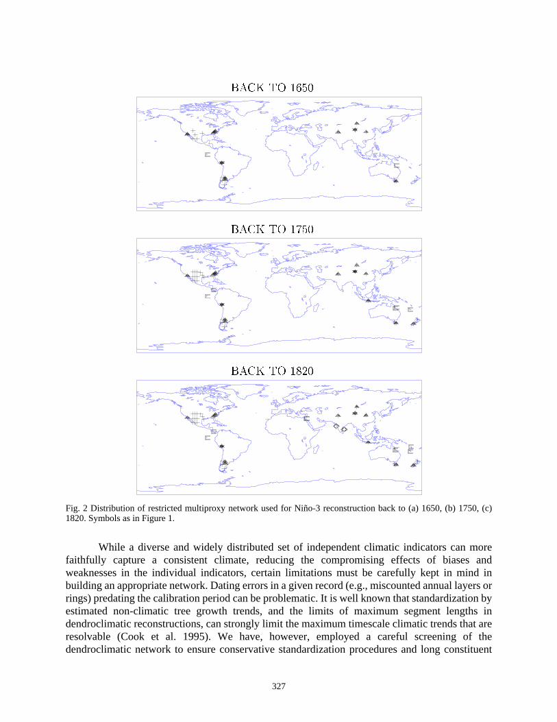
We employ a multiproxy network consisting of diverse high-quality annual resoluproxy climate indicators and long historical or instrumental records collected and analyzemany different paleoclimatologists (details provided in Table 1). All data have annual resol(or represent annual means in the case of instrumental data available at monthly resolution)gaps were interpolated and any records which terminate slightly before the end of the 19calibration interval (see “Method”) are extended by using persistence to 1980. Certainnetworks of the full multiproxy data network (e.g., regional dendroclimatic networks) have brepresented by a smaller number of their leading principal components (PCs), the maxnumber of which (available back to 1820) is indicated in parentheses, to ensure a more regglobally homogenous network. Two different sets of calibration experiments are performedfirst set uses the entire global multiproxy network (Fig. 1; this is essentially the same networkby MBH98) to reconstruct the “global ENSO” signal, while a more restricted “tropical” netw(Fig. 2) of indicators in tropical regions or subtropical regions most consistently impacteENSO is used to reconstruct the specific tropical Pacific El Niño signal. In using larindependent networks to describe both the global ENSO and the tropical El Niño signals, wable to independently assess both the tropical and global ENSO histories. We thereby in laravoid the potentially flawed assumption of a stationary extratropical response to tropical Eforcing.

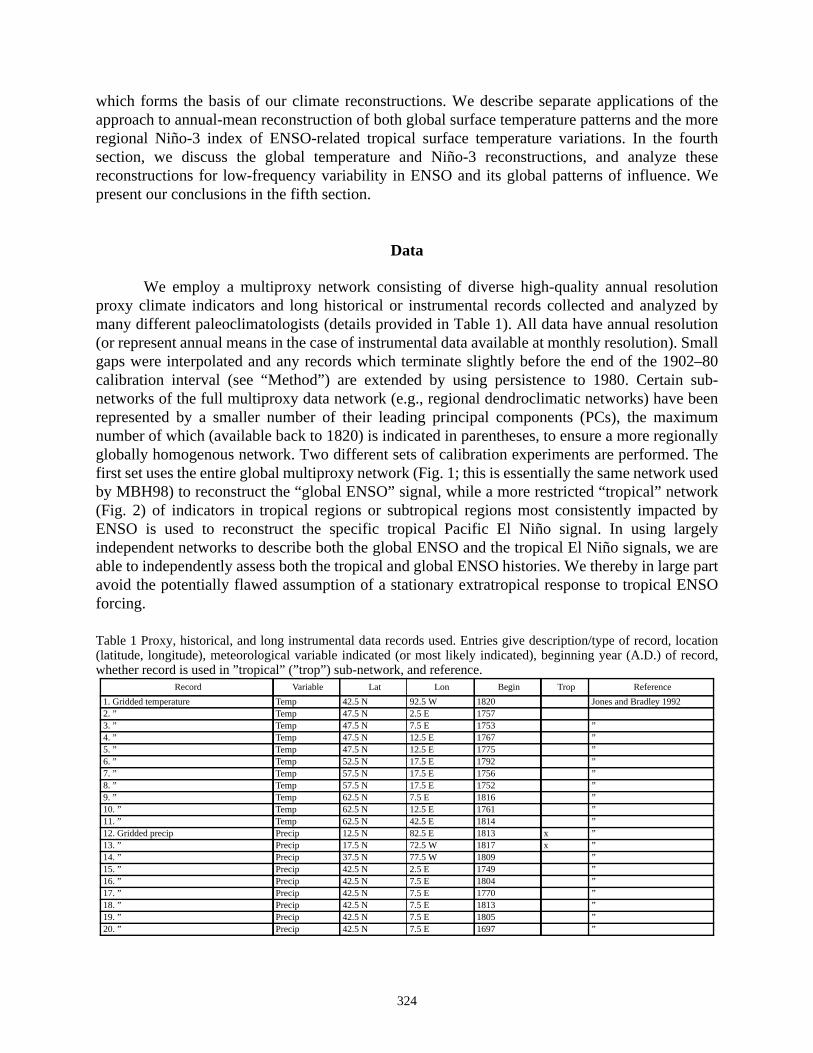
Table 1 Proxy, historical, and long instrumental data records used. Entries give description/type of record, lo(latitude, longitude), meteorological variable indicated (or most likely indicated), beginning year (A.D.) of rewhether record is used in ”tropical” (”trop”) sub-network, and reference.

Record Variable Lat Lon Begin Trop Reference

1. Gridded temperature Temp 42.5 N 92.5 W 1820 Jones and Bradley 19922. ” Temp 47.5 N 2.5 E 17573. ” Temp 47.5 N 7.5 E 1753 ”4. ” Temp 47.5 N 12.5 E 1767 ”5. ” Temp 47.5 N 12.5 E 1775 ”6. ” Temp 52.5 N 17.5 E 1792 ”7. ” Temp 57.5 N 17.5 E 1756 ”8. ” Temp 57.5 N 17.5 E 1752 ”9. ” Temp 62.5 N 7.5 E 1816 ”10. ” Temp 62.5 N 12.5 E 1761 ”11. ” Temp 62.5 N 42.5 E 1814 ”12. Gridded precip Precip 12.5 N 82.5 E 1813 x ”13. ” Precip 17.5 N 72.5 W 1817 x ”14. ” Precip 37.5 N 77.5 W 1809 ”15. ” Precip 42.5 N 2.5 E 1749 ”16. ” Precip 42.5 N 7.5 E 1804 ”17. ” Precip 42.5 N 7.5 E 1770 ”18. ” Precip 42.5 N 7.5 E 1813 ”19. ” Precip 42.5 N 7.5 E 1805 ”20. ” Precip 42.5 N 7.5 E 1697 ”

324

record,.) of

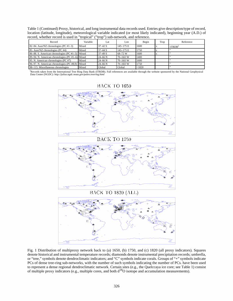
Table 1 (Continued) Proxy, historical, and long instrumental data records used. Entries give description/type oflocation (latitude, longitude), meteorological variable indicated (or most likely indicated), beginning year (A.Drecord, whether record is used in ”tropical” (”trop”) sub-network, and reference.

Record Variable Lat Lon Begin Trop Reference

21. ” Precip 42.5 N 7.5 E 1809 ”22. ” Precip 42.5 N 7.5 E 1785 ”

Historical

23. Cent England temp Temp 52 N 0 E 1730 Manley 195924. Cent Europe temp Temp 45 N 10 E 1550 Pfister 1992

Coral

25. Burdekin River (fluoresc) Precip/runoff 20 S 147 E 1746 x Lough 1991

26. Galapagos Isabel Island (d18O) SST 1 S 91 W 1607 x Dunbar et al. 1994

27. Gulf of Chiriqui, Panama (d18O) Precip 7.5 N 81 W 1708 x Linsley et al. 1994

28. Gulf of Chiriqui, Panama (d18 C) Ocean circ x

29. Espiritu Santu (d18O) SST 15 S 167 E 1806 x Quinn et al. 1993

30. New Caledonia (d18O) SST 22 S 166 E 1658 x Quinn et al. 1996

31. Great Barrier Reef (band thickness) SST 19 S 148 E 1615 x Lough, pers. comm.

32. Red Sea (d18O) SST/precip 29.5 N 35 E 1788 x Heiss 1994

33. Red Sea (d18C) Ocean circ x

Ice Core

34. Quelccaya summit ice core (d180) (Air temp) 14 S 71 W 470 x Thompson 1992

35. Quelccaya summit ice core (accum) Precip 488 x ”

36. Quelccaya ice core 2 (d18O) (Air temp) 744 x ”

37. Quelccaya ice core 2 (accum) Precip x ”

38. Dunde ice core (d18O) (Air temp) 38 N 96 E 1606 x Thompson 1992

39. Southern Greenland ice core (melt) Summer temp 66 N 45 W 1545 Kameda et al. 199640. Svalbard ice core (melt) Summer temp 79 N 17 W 1400 Tarussov 1992

41. Penny ice core (d18O) (Air temp) 70 N 70 W 1718 Fisher et al. 1998

42. Central Greenland stack (d18O) (Air temp) 77 N 60 W 553 Fisher et al. 1996

Dendroclimatic

43. Upper Kolyma River (ring widths) Temp 68 N 155 E 1550 Schweingruber, pers. comm.44. Java teak (ring widths) Precip 8 S 113 E 1746 x Jacoby and D'Arrigo 199045. Tasmanian Huon Pine (ring widths) Temp 43 S 148 E 900 x Cook et al. 199146. New Zealand S. Island (ring widths) Temp 44 S 170 E 1730 x Norton and Palmer 199247. Central Patagonia (ring widths) Temp 41 S 68 W 1500 x Boninsegna 199248. Fernoscandian Scots Pine (density) Temp 68 N 23 E 500 Briffa et al. 1992a49. Northern Urals (density) Temp 67 N 65 E 914 Briffa et al. 199550. Western North America (ring widths) Temp 39 N 111 W 1602 Fritts and Shao 199251. North American tree line (ring widths) Temp 69 N 163 W 1515 Jacoby and D'Arrigo 198952. ” Temp 66 N 157 W 1586 ”53. ” Temp 68 N 142 W 1580 ”54. ” Temp 64 N 137 W 1459 ”55. ” Temp 66 N 132 W 1626 ”56. ” Temp 68 N 115 W 1428 ”57. ” Temp 64 N 102 W 1491 ”58. ” Temp 58 N 93 W 1650 ”59. ” Temp 57 N 77 W 1663 ”60. ” Temp 59 N 71 W 1641 ”61. ” Temp 48 N 66 W 1400 ”62. S.E. U.S., N. Carolina (ring widths) Precip 36 N 80 W 1005 x Stahle et al. 198863. S.E. U.S., S. Carolina (ring widths) Precip 34 N 81 W 1005 x ”64. S.E. U.S., Georgia (ring widths) Precip 33 N 83 W 1005 x ”65. Mongolian Siberian Pine (ring widths) Precip 48 N 100 E 1550 x Jacoby et al. 199666. Yakutia (ring widths) Temp 62 N 130 E 1400 Hughes et al. 199867. OK/TX U.S. ring widths (PC #1) Precip 29–37 N 94–99 W 1600 x Stahle and Cleaveland 199368–69. OK/TX U.S. ring widths (PC #2,3) Precip 29–37 N 94–99 W 1700 x ”70. S.W. U.S./Mex widths (PC #l) Precip 24–37 N 103–109 W 1400 x ”71. S.W. U.S./Mex widths (PC #2) Precip 24–37 N 103–109 W 1500 x ”72–73. S.W. U.S./Mex widths (PC #3,4) Precip 24–37 N 103–109 W 1600 x ”74–76. S.W. U.S./Mex widths (PC #5–7) Precip 24–37 N 103–109 W 1700 x ”77–78. S.W. U.S./Mex widths (PC #8,9) Precip 24–37 N 103–109 W 1700 x ”79. Eurasian tree line ring widths (PC #1) Temp 60–70 N 100–180 E 1450 Vaganov et al. 199680. Eurasian tree line ring widths (PC #2) Temp 60–70 N 100–180 E 1600 ”81. Eurasian tree line ring widths (PC #3) Temp 60–70 N 100–180 E 1750 ”

325

record,.) of

hy

aresmbrella,icateen used) consist

Table 1 (Continued) Proxy, historical, and long instrumental data records used. Entries give description/type oflocation (latitude, longitude), meteorological variable indicated (or most likely indicated), beginning year (A.Drecord, whether record is used in ”tropical” (”trop”) sub-network, and reference.

1Records taken from the International Tree Ring Data Bank (ITRDB). Full references are available through the website sponsored by the National GeopsicalData Center (NGDC):http://julius.ngdc.noaa.gov/paleo.treering.html

Fig. 1 Distribution of multiproxy network back to (a) 1650, (b) 1750, and (c) 1820 (all proxy indicators). Squdenote historical and instrumental temperature records; diamonds denote instrumental precipitation records; uor “tree,” symbols denote dendroclimatic indicators; and “C” symbols indicate corals. Groups of “+” symbols indPCs of dense tree-ring sub-networks, with the number of such symbols indicating the number of PCs. have beto represent a dense regional dendroclimatic network. Certain sites (e.g., the Quelccaya ice core; see Table 1of multiple proxy indicators (e.g., multiple cores, and both d18O isotope and accumulation measurements).

Record Variable Lat Lon Begin Trop Reference

82–84. Aust/NZ chronologies (PC #1–3) Mixed 37–42 S 145–175 E 1600 x 1TRDB1

85. Aust/NZ chronologies (PC #4) Mixed 37–44 S 145–175 E 1750 x ”86–88. S. American chronologies (PC #1–3) Mixed 37–49 S 68–72 W 1600 x ”89–94. N. American chronologies (PC #1–6) Mixed 24–66 N 70–16O W 1400 ”95. N. American chronologies (PC #7) Mixed 24–66 N 70–16O W 1600 ”96–97. N. American chronologies (PC #8,9) Mixed 24–66 N 70–16O W 1750 ”98–115. Miscellaneous chronologies Mixed Global Global <1820 ”

BACK TO 1650

BACK TO 1750

BACK TO 1820 (ALL)

326

, (c)

oreand

d iners orn bys int aref thetituent

Fig. 2 Distribution of restricted multiproxy network used for Niño-3 reconstruction back to (a) 1650, (b) 17501820. Symbols as in Figure 1.

While a diverse and widely distributed set of independent climatic indicators can mfaithfully capture a consistent climate, reducing the compromising effects of biasesweaknesses in the individual indicators, certain limitations must be carefully kept in minbuilding an appropriate network. Dating errors in a given record (e.g., miscounted annual layrings) predating the calibration period can be problematic. It is well known that standardizatioestimated non-climatic tree growth trends, and the limits of maximum segment lengthdendroclimatic reconstructions, can strongly limit the maximum timescale climatic trends tharesolvable (Cook et al. 1995). We have, however, employed a careful screening odendroclimatic network to ensure conservative standardization procedures and long cons

BACK TO 1650

BACK TO 1750

BACK TO 1820

327

solvedand.

ude) withentale usepicall

ns of(NH)

orthernver thethe 100ºW

, theilable. Thehich

rly gridto at

ailabletinuousmeannd globale smallpointx (see

segment lengths, and variations on century and even multiple-century timescales are retypically. An analysis of the resolvability of multicentury timescale trends in these dataimplications for long-term climate reconstruction is provided elsewhere (Mann et al. 1998b)

To calibrate the multiproxy networks, we make use of all available grid point (5 longitby 5 latitude) land air and sea surface temperature anomaly data (Jones and Briffa 1992nearly continuous monthly sampling back to at least 1902. Short gaps in the monthly instrumdata are filled by linear interpolation. For the global temperature pattern reconstructions, wall (M = 1082) available nearly continuous grid point data available back to 1902. For troPacific SST/Niño reconstructions, we use the availableM = 121 SST grid point data in the tropicaPacific region bounded by the two tropics and the longitudes 115°E to 80°W. These data are shownin Figure 3. Although there are notable gaps in the spatial sampling, significant enough portiothe globe are sampled to estimate (in the case of the global field) the Northern Hemispheremean temperature series, and in both cases, the Niño-3 index of the El Niño phenomenon. NHemisphere temperature is estimated as areally weighted (i.e., cosine latitude) averages oNorthern Hemisphere. The Niño-3 eastern equatorial Pacific SST index is constructed fromgrid points available over the conventional Niño-3 box (see Fig. 3) for the region 5ºS to 5ºN, 9to 150ºW. While this spatial sampling covers only about one-third of the total Niño-3 regionassociated time series is nearly identical to the fully sampled Niño-3 region time series ava(both series share 90% of their variance in common during their overlap back to 1953)(negative) correlation of our Niño-3 average with the SOI—an alternative ENSO indicator wtends to covary oppositely with El Niño—is consistently high (r2 ≈ 0.5) and robust throughout thetwentieth century for the intervals during which both are available (0.44≤ r2 ≤ 0.51 for each of the1902–49, 1950–80, 1950–93, and 1902–93 intervals). We thus assert that the sparser eapoint SST data in the eastern tropical Pacific are sufficient for a reliable Niño-3 index backleast 1902.

Fig. 3 Distribution of the (1082) nearly continuous available land air/sea surface temperature grid point data avfrom 1902 onward, indicated by shading. The squares indicate the subset of 219 grid points, with nearly conrecords extending back to 1854 that are used for verification. Northern Hemisphere (NH) and global (GLB)temperature are estimated as areally weighted (i.e., cosine latitude) averages over the Northern Hemisphere adomains, respectively. The large rectangle indicates the tropical Pacific sub-domain discussed in the text. Threctangle in the eastern tropical Pacific shows the traditional Niño-3 region. An arithmetic mean of gridanomalies in our sampling of the Niño-3 region provides a reliable estimate of the fully sampled Niño-3 indetext for discussion).

328

tternsughesntary

l andlimate

orkd. Intworkt theataical”

fined

sionhes to1988),dataproxyiew).neousricalrentty oferentweessionion oflation

e. Ittheir

torsntieth-whichlve

rns areation

) thatationmptiontypical

tion),

Method

The advantage of using multiproxy data networks in describing and reconstructing paof long-term climate variability has been discussed elsewhere (Bradley and Jones 1993; Hand Diaz 1994; Mann et al. 1995; Mann et al. 1998a,b,c) and relies upon the complemecharacteristics and spatial sampling provided by a combined network of long historicainstrumental records, dendroclimatic, coral, and ice core–based climate proxy indicators of cchange. In our approach to climate field reconstruction, we seek to “train” the multiproxy netwby calibrating it against the dominant patterns of variability in the modern instrumental recorthe case of the global temperature field reconstructions, we use the entire multiproxy neshown earlier in Figure 1, and we “train” this network by calibrating it, series-by-series, againsdominant global patterns of temperature variability using the full sampling of grid point dshown in Figure 3. In the case of Niño-3 index reconstruction, we use the restricted “tropmultiproxy network (Fig. 2) and train it against the dominant patterns of SST variations conto the tropical Pacific sub-domain (see region indicated in Fig. 3).

The calibration of the multiproxy network is accomplished by a multivariate regresagainst instrumental temperature data. Conventional multivariate regression approacpaleoclimate reconstruction, such as canonical correlation analysis (CCA; see Preisendorferwhich simultaneously decompose both the proxy “predictor” and instrumental “predictand”in the regression process, work well when applied to relatively homogeneous networks ofdata (e.g., regional dendroclimatic networks; see Cook et al. 1994 for an excellent revHowever, we found that such approaches were not effective with the far more inhomogemultiproxy data networks. Different types of proxies (e.g., tree rings, ice cores, and historecords) differ considerably in their statistical properties, reflecting, for example, diffeseasonal windows of variability, and exhibiting different spectral attributes in their resolvabiliclimatic variations. Thus, rather than seeking to combine the disparate information from diffproxy indicators initially through a multivariate decomposition of the proxy network itself,instead choose to use the information contained in the network in a later stage of the regrprocess. Our approach is similar, in principle, to methods applied recently to the reconstructearly instrumental temperature fields from sparse data, based on eigenvector interpotechniques (Smith et al. 1996; Kaplan et al. 1998).

Our calibration approach, which was described in MBH98, is further detailed herinvolves first decomposing the twentieth-century instrumental surface temperature data intodominant patterns of variability or “eigenvectors.” Second, the individual climate proxy indicaare regressed against the time histories of these distinct patterns during their shared twecentury interval of overlap. One can think of the instrumental patterns as templates againstwe “train” the much longer proxy “predictor.” This calibration process allows us, finally, to soan “inverse problem” whereby the closest-match estimates of surface temperature pattededuced back in time before the calibration period, on a year-by-year basis, based on informin the multiproxy network.

At least three fundamental assumptions are implicit in this approach. We assume (1the indicators in our multiproxy trainee network are statistically related to some linear combinof the eigenvectors of the instrumental global annual-mean temperature data. This assucontrasts with that of typical paleoclimate calibration approaches. Rather than seeking, as instudies, to relate a particular proxy record locally to an at-site instrumental record of somea prioriselected meteorological variable (e.g., temperature, precipitation, or atmospheric wind direc

329

ictiveroxyimatences.sone-ring-asonlationhavemplexof the

e ouratic

ich theBriffa

that amaycales

thelessthernalens of

thenaritysome

e thatstes ofat leasttisticalals, asurposes

s thes. Thelobal

and, ine dataapply

rmed

ndard

during somea priori selected seasonal (e.g., summer) window, we make instead a less restrassumption that whatever combination of local meteorological variables influence the precord, they find expression in one or more of the largest-scale patterns of annual clvariability. Ice core and coral proxy indicators reflect, in general, a variety of seasonal influeMany extratropical tree-ring (ring widths and density) series primarily reflect warm-seatemperature influences (see, e.g., Schweingruber et al. 1991; Bradley and Jones 1993). Trewidth series in subtropical semiarid regions, however, are reflective in large part of cold-seprecipitation influences. These influences are, in turn, tied to larger-scale atmospheric circuvariations (e.g., the PNA or NAO atmospheric patterns; see, e.g., D'Arrigo et al. 1993) thatimportant influences on large-scale temperature. When a proxy indicator represents some cocombination of local meteorological and seasonal influences, we make more complete useavailable information in the calibration process than do conventional approaches. Whilmethod seeks only to recognize that variability in the proxy data tied to large-scale climpatterns, it appears that temperature variability at interannual and longer timescales, for wheffective number of spatial degrees of freedom are greatly reduced (see, e.g., Jones and1992), is inherently large-scale in nature. This latter observation underlies our assertion (2)relatively sparse but widely distributed sampling of long proxy and instrumental recordssample much of the large-scale variability that is important at interannual and longer times(see also Bradley 1996). Regions not directly represented in the trainee network may nonebe indirectly represented through teleconnections with regions that are. The El Niño/SouOscillation is itself an example of a pattern of climatic variability which exhibits global-scinfluence (e.g., Halpert and Ropelewski 1992). Finally, we assume (3) that the pattervariability captured by the multiproxy network have analogs in the patterns we resolve inshorter instrumental data. This latter assumption represents a fairly weak statiorequirement—we do not require that the climate itself be stationary. In fact, we expect thatsizable trends in the climate may be resolved by our reconstructions. We do, however, assumthe fundamentalspatial patternsof variation which the climate has exhibited during the pacentury are similar to those by which it has varied during past recent centuries. Studiinstrumental surface temperature patterns suggest that such a form of stationarity holds upon multidecadal timescales, during the past century (Kaplan et al. 1998). Independent stacross-validation exercises and careful examination of the properties of the calibration residudescribed later, provide the best evidence that these key assumptions hold, at least for the pof our reconstructions of temperature patterns during the past few centuries.

The first step in the pattern reconstruction process, as discussed above, idecomposition of the modern instrumental data into its dominant spatiotemporal eigenvectorN = 1104 monthly samples available between 1902 and 1993 are sufficient for both the gtemperature field (theM = 1082 grid point series described in the “Data” section; see Fig. 3)the M' = 121 grid point series in the tropical Pacific region used in Niño-3 reconstructionproviding a unique, well-posed eigendecomposition of the instrumental surface temperaturinto its leading empirical eigenvectors. The method as described henceforth is understood toboth the global pattern and tropical Pacific SST/Niño-3 reconstructions, which are perfoindependently.

For each grid point, the mean was removed, and the series was normalized by its stadeviation. The standardized data matrix can be written,

330

that

data

n

thes (Fig.in the, 5 =andof thespatialanceoballassiclies inorth

ns ofgativeet al.of thesitivethird

basincadalthis1990sectorpical

wheret1, t2, …tN spans over theN = 1104 months, andm = 1, 2, …,M spans theM = 1082 gridpoints.wm indicates weighting by the cosine of the central latitude of each grid point to ensuregrid points contribute in proportion to the area represented.

A standard principal component analysis (PCA) is then applied to the standardizedmatrix ,

decomposing the data set into its dominant spatiotemporal eigenvectors. TheM-vector or empiricalorthogonal function (EOF)vk describes the relative spatial pattern of thekth eigenvector, the N-vectoruk or PC describes its variation over time, and the scalarlk describes the associated fractioof resolved (standardized and weighted) data variance.

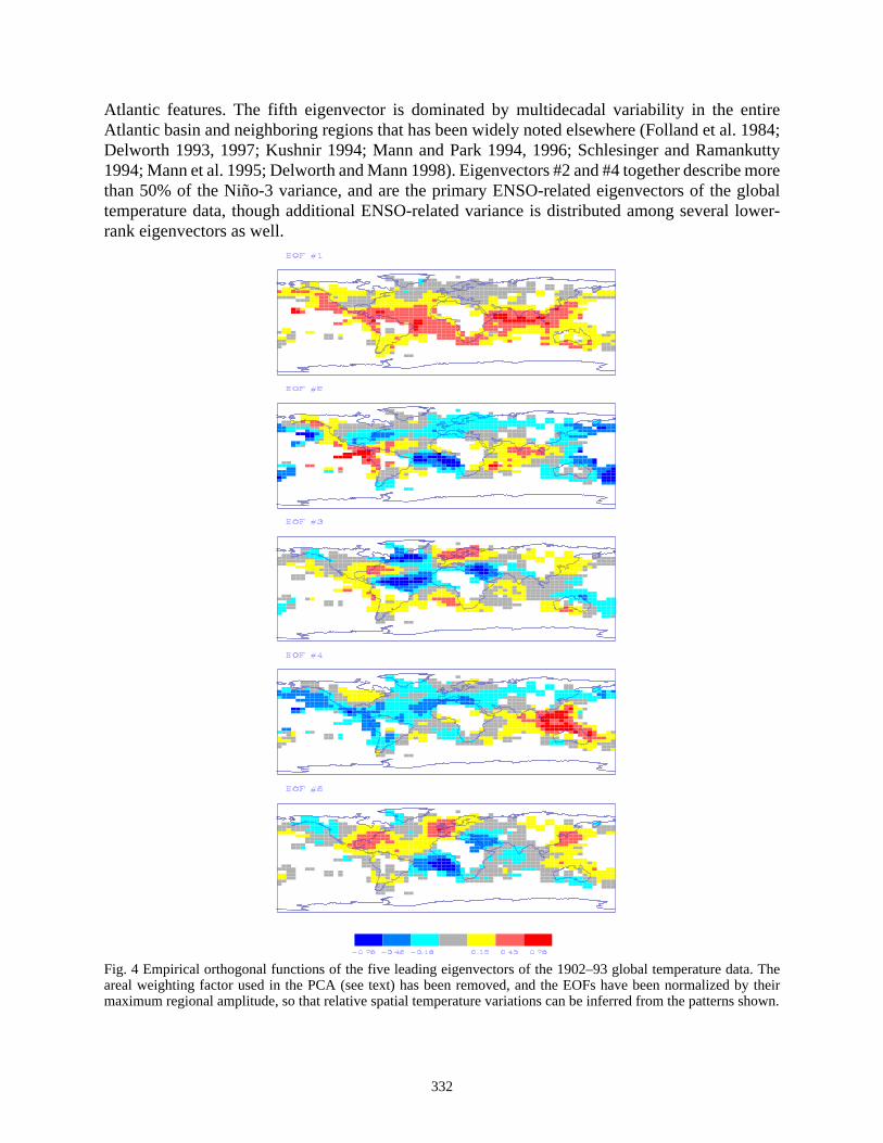
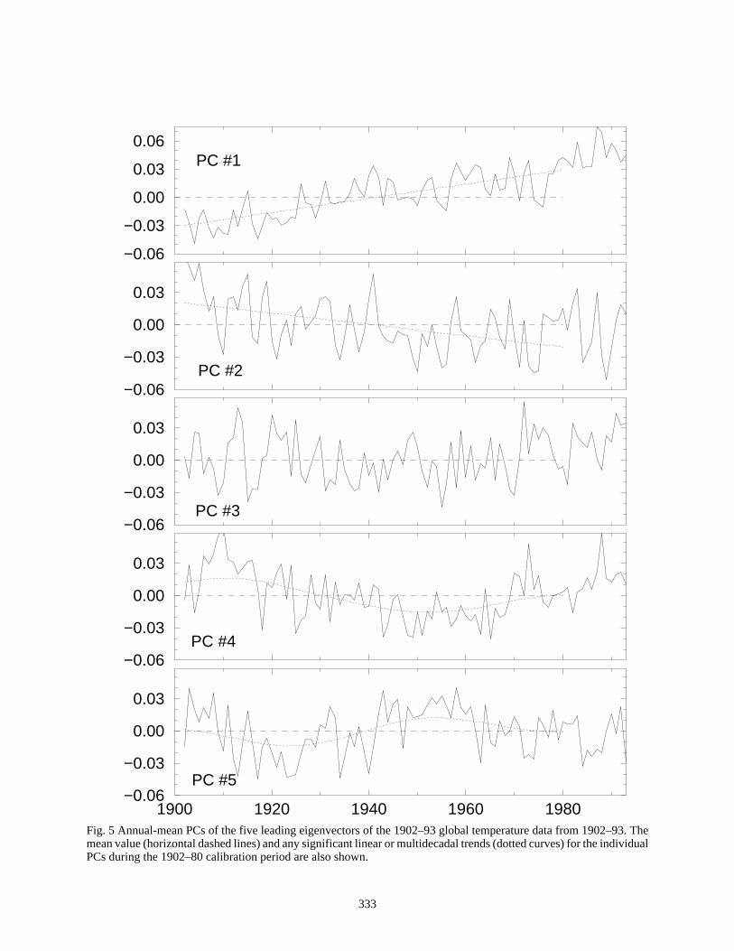
The first five eigenvectors of the global temperature data are particularly important inglobal temperature pattern reconstructions, as is described later. The EOFs (Fig. 4) and PC5) are shown for these five eigenvectors, in decreasing order of the variance they explainglobal instrumental temperature data shown in Figure 3 (1 = 12%, 2 = 6.5%, 3 = 5%, 4 = 4%3.5%). The first eigenvector describes much of the variability in the global (GLB = 88%)hemispheric (NH = 73%) means, and is associated with the significant global warming trendpast century (see Fig. 5). Subsequent eigenvectors, in contrast, describe much of thevariability relative to the large-scale means (i.e., much of the remaining multivariate vari“MULT”). The second eigenvector is the dominant ENSO-related component of the gltemperature data, describing 41% of the variance in the Niño-3 index, and exhibiting certain cextratropical ENSO signatures (e.g., the “horseshoe” pattern of warm and cold SST anomathe North Pacific, and an anomaly pattern over North America reminiscent of the Pacific-NAmerican (PNA) or related Tropical/Northern Hemisphere (TNH) atmospheric teleconnectioENSO; see Barnston and Livezey [1987]). This eigenvector exhibits a modest long-term netrend, which, in the eastern tropical Pacific, describes a La Niña–like cooling trend (Cane1997) that opposes warming in the same region associated with the global warming patternfirst eigenvector. This cooling trend has been punctuated recently, however, by a few large poexcursions (see Fig. 5) associated with the large El Niños of the 1980s and 1990s. Theeigenvector is associated largely with interannual- to decadal-scale variability in the Atlanticand carries the well-known temperature signature of the North Atlantic Oscillation and detropical Atlantic variability (e.g., Chang et al. 1997). While there is no long-term trend inpattern during the twentieth century, a recent decadal-scale upturn during the late 1980s towhich has been noted elsewhere (see Hurrell 1995) is evident (Fig. 5). The fourth eigenvdescribes a primarily multidecadal timescale variation with ENSO-scale and tropical/subtro

T

w1T1( )t1

w2T2( )t1

…wMTM( )t1

w1T1( )t2

w2T2( )t2

…wMTM( )t2

…

w1T1( )

tNw2T

2( )tN

…wMTM( )tN

=

T

T λkukvkk 1=

K

∑=

331

tire1984;kuttymorelobal

lower-

a. Theby their shown.

Atlantic features. The fifth eigenvector is dominated by multidecadal variability in the enAtlantic basin and neighboring regions that has been widely noted elsewhere (Folland et al.Delworth 1993, 1997; Kushnir 1994; Mann and Park 1994, 1996; Schlesinger and Raman1994; Mann et al. 1995; Delworth and Mann 1998). Eigenvectors #2 and #4 together describethan 50% of the Niño-3 variance, and are the primary ENSO-related eigenvectors of the gtemperature data, though additional ENSO-related variance is distributed among severalrank eigenvectors as well.

Fig. 4 Empirical orthogonal functions of the five leading eigenvectors of the 1902–93 global temperature datareal weighting factor used in the PCA (see text) has been removed, and the EOFs have been normalizedmaximum regional amplitude, so that relative spatial temperature variations can be inferred from the patterns

332

3. Theividual

Fig. 5 Annual-mean PCs of the five leading eigenvectors of the 1902–93 global temperature data from 1902–9mean value (horizontal dashed lines) and any significant linear or multidecadal trends (dotted curves) for the indPCs during the 1902–80 calibration period are also shown.

1900 1920 1940 1960 1980−0.06

−0.03

0.00

0.03

−0.06

−0.03

0.00

0.03

−0.06

−0.03

0.00

0.03

−0.06

−0.03

0.00

0.03

−0.06

−0.03

0.00

0.03

0.06PC #1

PC #2

PC #3

PC #4

PC #5

333

threee 50%parsebility.do thee theannualctorlobal

opical

actual) the

stru-f

(NIN),s (

ecordsb,

the

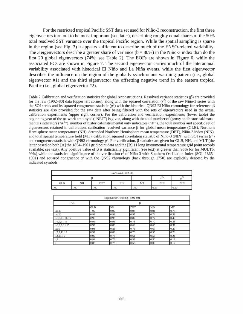
For the restricted tropical Pacific SST data set used for Niño-3 reconstruction, the firsteigenvectors turn out to be most important (see later), describing roughly equal shares of thtotal resolved SST variance over the tropical Pacific region. While the spatial sampling is sin the region (see Fig. 3) it appears sufficient to describe much of the ENSO-related variaThe 3 eigenvectors describe a greater share of variance (b = 80%) in the Niño-3 index thanfirst 20 global eigenvectors (74%; see Table 2). The EOFs are shown in Figure 6, whilassociated PCs are shown in Figure 7. The second eigenvector carries much of the intervariability associated with historical El Niño and La Niña events, while the first eigenvedescribes the influence on the region of the globally synchronous warming pattern (i.e., geigenvector #1) and the third eigenvector the offsetting negative trend in the eastern trPacific (i.e., global eigenvector #2).

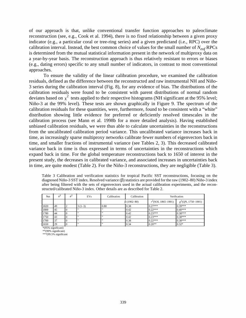
Table 2 Calibration and verification statistics for global reconstructions. Resolved variance statistics (β) are providedfor the raw (1902–80) data (upper left corner), along with the squared correlation (r2) of the raw Niño-3 series withthe SOI series and its squared congruence statistic (g2) with the historical QN92 El Niño chronology for reference.βstatistics are also provided for the raw data after being filtered with the sets of eigenvectors used in thecalibration experiments (upper right corner). For the calibration and verification experiments (lower tablebeginning year of the network employed (“NET”) is given, along with the total number of (proxy and historical/inmental) indicators (“#T”), number of historical/instrumental only indicators (“#I”), the total number and specific set oeigenvectors retained in calibration, calibration resolved varianceβ for global mean temperature (GLB), NorthernHemisphere mean temperature (NH), detrended Northern Hemisphere mean temperature (DET), Niño-3 indexand total spatial temperature field (MT), calibration squared correlation statistic of Niño-3 (NIN) with SOI serier2)and congruence statistic with QN92 chronologyg2. For verification,β statistics are given for GLB, NH, and MLT (thelatter based on both [A] the 1854–1901 grid point data and the [B] 11 long instrumental temperature grid point ravailable; see text). Any positive value ofβ is statistically significant (see text) at greater than 95% (or for MULT99%) while the statistical significance of the verificationr2 of Niño-3 with Southern Oscillation Index (SOI, 1865–1901) and squared congruenceg2 with the QN92 chronology (back through 1750) are explicitly denoted byindicated symbols.

Raw Data (1902-08)

β r2a g2b

GLB NH DET NIN MT NIN NIN

1.00 1.00 1.00 1.00 1.00 0.51 0.50

Eigenvector Filtering (1902-80)

EVs βGLB NH DET NIN MT

1st 40 1.00 0.99 0.98 0.91 0.731st 20 0.99 0.99 0.97 0.74 0.581-5,9,11,14-16 0.95 0.93 0.87 0.72 0.401-5,9,11,15 0.95 0.93 0.78 0.70 0.381-3,6,8,11,15 0.92 0.83 0.69 0.65 0.311st 5 0.93 0.85 0.76 0.67 0.271,2,5,11,15 0.92 0.83 0.70 0.55 0.231,2,11,15 0.90 0.78 0.61 0.53 0.211,2 0.91 0.76 0.57 0.50 0.181 0.88 0.73 0.53 0.09 0.12

334

region

Table 2 (Continued)

+ (85% significant); * (90% significant); ** (95% significant); *** (99% significant); x (unphysical positive correlation obtained)a (r2 with SOI);b (g2 w/QN92 chron)1 (no instrumental/historical data—proxy only;2 (instrumental/historical data only);3 (dendroclimatic indicators excluded)

Fig. 6 Empirical orthogonal functions of the three leading eigenvectors of the 1902–93 restricted tropical Pacifictemperature data. Color-scale and other conventions are as in Figure 4.

Calibration (1902-80) Verification (pre-1902)

Net #T #T β r2 g2 β r2 g2

GLB NH DET NIN MT NIN NIN GLB NH MTa MTb NIN NIN

1820 112 24 11 (1–5,7,9,11,14–16) 0.77 0.76 0.56 0.48 0.30 0.51 0.29 0.76 0.69 0.22 0.55 0.14** 0.28**1800 102 15 “ 0.76 0.75 0.54 0.50 0.27 0.52 0.30 0.75 0.68 0.19 0.45 0.10** 0.22**1780 97 12 “ 0.76 0.74 0.54 0.51 0.27 0.53 0.29 0.76 0.69 0.17 0.40 0.11** 0.20**1760 93 8 9 (1–5,7,9,11,15) 0.76 0.74 0.52 0.49 0.26 0.52 0.29 0.75 0.70 0.17 0.33 0.10** 0.17*1750 89 5 8 (1–3,5,6,8,11,15) 0.76 0.74 0.53 0.34 0.18 0.39 0.33 0.64 0.57 0.11 0.13 0.10** 0.19*1730 79 3 5 (1,2,5,11,15) 0.74 0.71 0.47 0.23 0.15 0.30 0.29 0.65 0.61 0.11 0.13 0.05* 0.17*1700 74 2 “ 0.74 0.71 0.47 0.22 0.14 0.29 0.29 0.63 0.57 0.10 0.12 0.05* 0.15+1650 57 1 4 (1,2,11,15) 0.72 0.67 0.42 0.05 0.14 0.19 0.23 0.61 0.53 0.12 0.10 0.02+ 0.11*

18201 88 0 8 (1–3,5,6,8,11,15) 0.76 0.73 0.51 0.31 0.19 0.37 0.31 0.65 0.56 0.11 0.19 0.12** 0.29*

18202 24 24 2 (1,2) 0.32 0.28 -0.28 -0.27 0.10 0.07 0.20 0.30 0.37 0.11 0.26 0.0 0.16

18203 42 24 7 (1–3,5,11,15,16) 0.50 0.50 0.13 0.05 0.17 0.22 0.18 0.56 0.53 0.17 0.47 0.09* 0.10

17503 19 2 2 (1,2) 0.46 0.47 0.05 0.2 0.09 0.30 0.27 0.28 0.27 0.06 0.10 0.03+ 0.15

335

eraturein the

Fig. 7 Annual-mean PCs of the three leading eigenvectors of the 1902–93 restricted tropical Pacific region tempdata. Conventions are as in Figure 5. Vertical dashed lines indicate the timing of El Niño events as recordedQN92 chronology.

1900 1920 1940 1960 1980YEAR

−0.05

0.00

0.05

−0.05

0.00

0.05

−0.05

0.00

0.05 PC #1 (trop Pac)

PC #2 (trop Pac)

PC #3 (trop Pac)

336

lity inem atditions,mates ofthat

rcise,ed PCs

ectivein thethe

patialariousce asion ofwhichthe

ctionsideredentlylow).

ng980s wereseries

roxy

termined

Having isolated the dominant spatiotemporal patterns of surface temperature variabithe instrumental record, we subsequently calibrate the multiproxy data networks against thannual mean resolution. As described above, we seek to reconstruct only annual-mean conexploiting the complementary information in data reflecting diverse seasonal windows of clivariability. The calibrations will provide a basis for reconstructing annual global patterntemperature back in time from the multiproxy network, with a spatial coverage dictated byavailable from the instrumental data the 1902–80 calibration period. In a given calibration exewe retain a specified subset of the annually averaged eigenvectors, the annually averagdenoted by , wheren = 1,..., , = 79 is the number of annual averages used of theN monthlength data set. In practice, only a small subsetNeofof the highest-rank eigenvectors turn out to buseful in these exercises from the standpoint of verifiable reconstructive skill. An objecriterion was used to determine the particular set of eigenvectors which should be usedcalibration as follows. Preisendorfer's (1988) selection rule, “rule N,” was applied tomultiproxy network to determine the approximate numberNeofof significant independent climaticpatterns that are resolved by the network, taking into account the approximate number of sdegrees of freedom represented by the multiproxy data set. Because the ordering of veigenvectors in terms of their prominence in the instrumental data, and their prominenrepresented by the multiproxy network, need not be the same, we allowed for the selectnoncontiguous sequences of the instrumental eigenvectors. We used an objective criterion inthe group ofNeof of the highest-rank instrumental eigenvectors was chosen which optimizedcalibration explained variance. Neither the measures of statistical skill nor the reconstruthemselves were highly sensitive to the precise criterion for selection, although it was consencouraging from a self-consistency point of view that the objective criterion independoptimized, or nearly optimized, the verification explained verification statistics (discussed be

TheseNeof eigenvectors were trained against theNproxy indicators, by finding the least-squares optimal combination of theNeof PCs represented by each individual proxy indicator durithe = 79 year training interval from 1902 to 1980 (the training interval is terminated at 1because many of the proxy series terminate at or shortly after 1980). The proxy series and PCformed into anomalies relative to the same 1902-08 reference period mean, and the proxywere also normalized by their standard deviations during that period. This proxy-by-pcalibration is well posed (i.e., a unique optimal solution exists) as long as >Neof (a limit neverapproached in this study) and can be expressed as the least-squares solution to the overdematrix equation,

is the matrix of annual PCs, and

unk

N N

N

N

Ux y p( )=

U

u11( )

u12( )…u1

Neof( )

u21( )

u22( )…u2

Neof( )

…

uN

1( )u

N2( )…u

N

Neof( )

=

337

d

tion

athere

s are

ctionsenotedal field,

ages.d thusre

is the time series –vector for proxy recordp.TheNeof-length solution vectorx = G(p) is obtained by solving the above overdetermine

optimization problem by singular value decomposition (SVD) for each proxy recordp = 1, . . . ,P.This yields a matrix of coefficients relating the different proxies to their closest linear combinaof theNeofPCs,

This matrix of coefficients cannot simultaneously be satisfied in the regression, but rrepresents a highly overdetermined relationship between the optimal weights on each of thNeofPCs and the information in the multiproxy network at any given time.

Proxy-reconstructed patterns for the global temperature and tropical Pacific SST fieldfinally obtained based on the year-by-year solution of the overdetermined matrix equation,

where y(j) is the predictor vector of values of each of theP proxy indicators during yearj. Thepredictand solution vector contains the least-squares optimal values of each of theNeofPCsfor a given year.

This yearly reconstruction process leads to annual sequences of the optimal reconstruof the retained PCs, which we term the reconstructed principal components, or RPCs, and dby uk. Once the RPCs are determined, the associated temperature patterns (of either the globor tropical Pacific SST) are readily obtained through the appropriate eigenvector expansion

while quantities of interest (e.g., NH, Niño-3) are calculated from the appropriate spatial averThe optimization procedure described above to yield the RPCs is overdetermined (an

well constrained) as long asP > Neof, which is always realized in this study. An important featu

y p( )

y 1p( )

y 2p( )

…

yN

p( )

=

N

G

G11( )

G21( )…GNeof

1( )

G12( )

G22( )…GNeof

2( )

…

G1P( )

G2P( )…GNeof

P( )

=

Gz y j( )=

z U=

T λkukvkk 1=

Neof

∑=

338

imateproxyer the

a onbiasestional

tionNiño-

f thedomlevel;f thehite”thelishedctions

ack inack inibratedwhichin theties backle 3).

thexrecon-

of our approach is that, unlike conventional transfer function approaches to paleoclreconstruction (see, e.g., Cook et al. 1994), there is no fixed relationship between a givenindicator (e.g., a particular coral or tree-ring series) and a given predictand (i.e., RPC) ovcalibration interval. Instead, the best common choice of values for the small number ofNeofRPCsis determined from the mutual statistical information present in the network of multiproxy data year-by-year basis. The reconstruction approach is thus relatively resistant to errors or(e.g., dating errors) specific to any small number of indicators, in contrast to most convenapproaches.

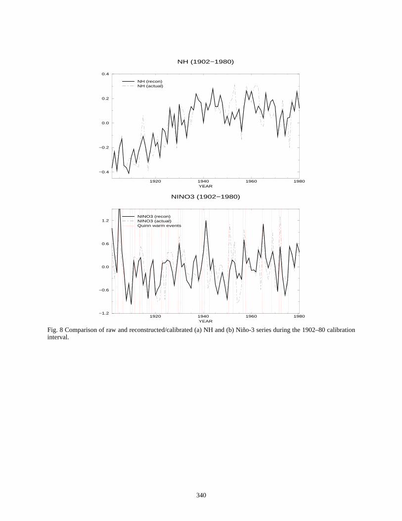
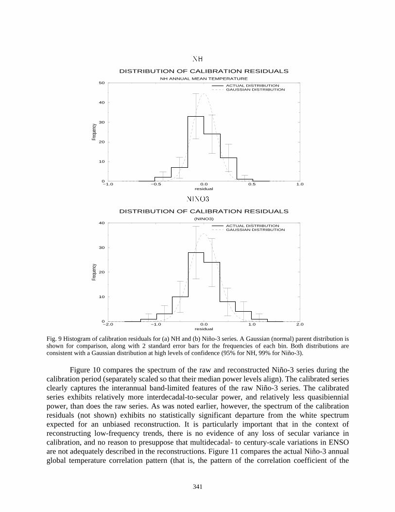
To ensure the validity of the linear calibration procedure, we examined the calibraresiduals, defined as the difference between the reconstructed and raw instrumental NH and3 series during the calibration interval (Fig. 8), for any evidence of bias. The distributions ocalibration residuals were found to be consistent with parent distributions of normal randeviates based on tests applied to their respective histograms (NH significant at the 95%Niño-3 at the 99% level). These tests are shown graphically in Figure 9. The spectrum ocalibration residuals for these quantities, were, furthermore, found to be consistent with a “wdistribution showing little evidence for preferred or deficiently resolved timescales incalibration process (see Mann et al. 1998b for a more detailed analysis). Having estabunbiased calibration residuals, we were thus able to calculate uncertainties in the reconstrufrom the uncalibrated calibration period variance. This uncalibrated variance increases btime, as increasingly sparse multiproxy networks calibrate fewer numbers of eigenvectors btime, and smaller fractions of instrumental variance (see Tables 2, 3). This decreased calvariance back in time is thus expressed in terms of uncertainties in the reconstructionsexpand back in time. For the global temperature reconstructions back to 1650 of interestpresent study, the decreases in calibrated variance, and associated increases in uncertainin time, are quite modest (Table 2). For the Niño-3 reconstructions, they are negligible (Tab

*(95% significant)**(99% significant)***(99.5% significant

Table 3 Calibration and verification statistics for tropical Pacific SST reconstructions, focusing ondiagnosed Niño-3 SST index. Resolved variance (β) statistics are provided for the raw (1902–80) Niño-3 indeafter being filtered with the sets of eigenvectors used in the actual calibration experiments, and thestructed/calibrated Niño-3 index. Other details are as described for Table 2.

Net #T #T EVs Calibration Calibration Verification

β (1902–80) r2(SOI, 1865–1901) g2(QN, 1750–1901)

1820 49 2 3 (1–3) 0.80 0.38 0.27*** 0.39***1800 45 0 ” ” 0.42 0.22*** 0.40***1780 44 0 ” ” 0.42 0.23*** 0.38***1750 43 0 ” ” 0.42 0.23*** 0.38***1700 37 0 ” ” 0.38 0.22*** 0.38***1650 29 0 ” ” 0.34 0.20** 0.32*

χ2

339

ration

Fig. 8 Comparison of raw and reconstructed/calibrated (a) NH and (b) Niño-3 series during the 1902–80 calibinterval.

1920 1940 1960 1980YEAR

−0.4

−0.2

0.0

0.2

0.4

NH (1902−1980)

NH (recon)NH (actual)

1920 1940 1960 1980YEAR

−1.2

−0.6

0.0

0.6

1.2

NINO3 (1902−1980)

NINO3 (recon)NINO3 (actual)Quinn warm events

340

ion isns are

g theseriesrated

ennialration

trumxt ofce inENSOannualf the

Fig. 9 Histogram of calibration residuals for (a) NH and (b) Niño-3 series. A Gaussian (normal) parent distributshown for comparison, along with 2 standard error bars for the frequencies of each bin. Both distributioconsistent with a Gaussian distribution at high levels of confidence (95% for NH, 99% for Niño-3).

Figure 10 compares the spectrum of the raw and reconstructed Niño-3 series durincalibration period (separately scaled so that their median power levels align). The calibratedclearly captures the interannual band-limited features of the raw Niño-3 series. The calibseries exhibits relatively more interdecadal-to-secular power, and relatively less quasibipower, than does the raw series. As was noted earlier, however, the spectrum of the calibresiduals (not shown) exhibits no statistically significant departure from the white specexpected for an unbiased reconstruction. It is particularly important that in the contereconstructing low-frequency trends, there is no evidence of any loss of secular variancalibration, and no reason to presuppose that multidecadal- to century-scale variations inare not adequately described in the reconstructions. Figure 11 compares the actual Niño-3global temperature correlation pattern (that is, the pattern of the correlation coefficient o

NH

−1.0 −0.5 0.0 0.5 1.0residual

0

10

20

30

40

50

Freq

uenc

y

DISTRIBUTION OF CALIBRATION RESIDUALSNH ANNUAL MEAN TEMPERATURE

ACTUAL DISTRIBUTIONGAUSSIAN DISTRIBUTION

NINO3

−2.0 −1.0 0.0 1.0 2.0residual

0

10

20

30

40

Freq

uenc

y

DISTRIBUTION OF CALIBRATION RESIDUALS(NINO3)

ACTUAL DISTRIBUTIONGAUSSIAN DISTRIBUTION

341

ationeriod.lationtion

902–80; Mann

annual Niño-3 index with the annual global temperature field reconstructions) with the correlpattern based on the multiproxy-reconstructed counterparts, for the 1902–80 calibration pThe multiproxy-based correlation pattern clearly captures the details of the observed correpattern during the calibration period, giving some justification to analyzing changing correlapatterns back in time from the reconstructions.

Fig. 10 Spectrum of raw instrumental (solid) and reconstructed/calibrated (dashed) Niño-3 series during the 1calibration period. The spectrum is calculated by using the multitaper method (Thomson 1982; Park et al. 1987and Lees 1996) based on three tapers and a time-frequency bandwidth product ofW = 2N.

0.0 0.1 0.2 0.3 0.4 0.5FREQUENCY (CYCLE/YR)

10

100

log

psd

NINO3 SPECTRUM (1902−1980)

actual raw datareconstructed

342

ructed/with a

a two-

ntlytion”ized in

Fig. 11 Niño-3 correlation map during1902–80 calibration period based on (top) raw data and (bottom) reconstcalibrated Niño-3 and global temperature patterns. The color scale indicates the specific level of correlationgiven grid point, with any color value outside of gray significant at greater than roughly the 80% level based onsided test. Red and blue indicated significance well above the ~99% confidence level.

The skill of the temperature reconstructions (i.e., their statistical validity) is independeestablished through a variety of complementary independent cross-validation or “verificaexercises. The numerical results of the calibration and verification experiments are summar

343

tionsused

atedig. 1)seriesilableh the

NSO-of Elns ofentalermiño-nd 3)the

a)l gridts [2]atistic

LB

ls forliableriod.m

armed fordardrisonsnNiño-

e

tionback

ack toables 2r to

(1998)moret here,n, we(e.g.,

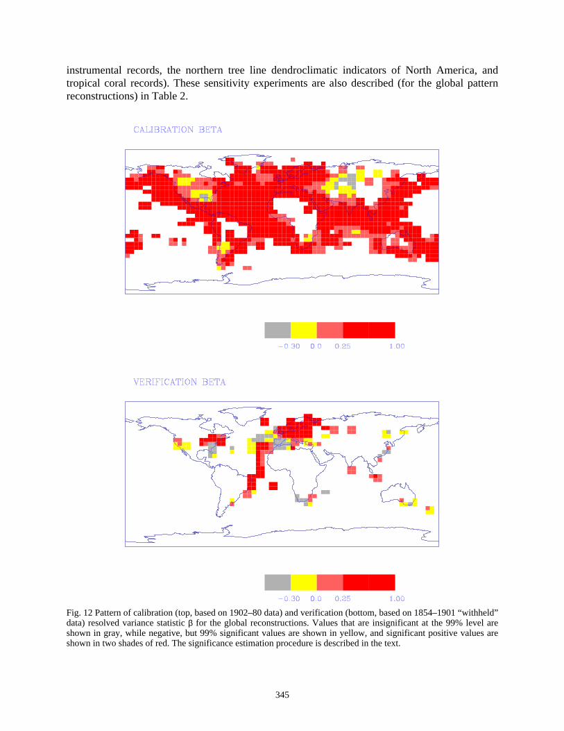
Table 2 for the global pattern reconstructions and in Table 3 for the Pacific SST reconstrucupon which the Niño-3 index is ultimately based. Four distinct sources of verification werefor the global reconstructions: (1) widespread instrumental grid point data (M′= 219 grid points;see Fig. 3) available for the period 1854–1901, (2) a small subset of 11 very long estiminstrumental temperature grid point averages (10 in Eurasia, 1 in North America; see Fconstructed from the longest available station measurement (each of these “grid point”shared at least 70% of their variance with the corresponding temperature grid point avaduring 1854–1980, providing verification back to at least 1820 in all cases (and back througmid- and early eighteenth century in many cases), (3) the SOI available for corroboration of Escale variability during the late nineteenth century, and (4) the QN92 historical chronologyNiño events dating back into the sixteenth century. Exercise (1) provides the only meawidespread instrumental spatial verification, but only experiment (3) provides instrumverification of the Niño-3 region, while exercises (2) and (4) address the fidelity of long-tvariability. Only verification experiments (3) and (4) were used to diagnose (in terms of the N3 index) the quality of the tropical Pacific pattern reconstructions. Note (compare Tables 2 athat the calibration and verification experiments indicate a more skillful Niño-3 index fromtropical Pacific SST-based reconstructions than from the global reconstructions.

The spatial patterns of described variance (β) for both calibration (based on 1902–80 datand verification (based on verification experiments [1] consisting of the withheld instrumentapoint data for 1854–1901) are shown for the global reconstructions in Figure 12. Experimenprovide a longer-term, albeit an even less spatially representative, multivariate verification st(“MULTb”). In this case, the spatial sampling does not permit meaningful estimates of NH or Gmean quantities. In any of these diagnostics, a positive value ofβ is statistically significant atgreater than 99% confidence as established from Monte Carlo simulations. Verification skilthe Niño-3 reconstructions were estimated indirectly by experiments [3] and [4], since a reinstrumental Niño-3 index was not available far beyond the beginning of the calibration peThe (negative) correlationr of Niño-3 with the SOI annual mean for 1865–1901 (obtained froP.D. Jones, personal communication) and a squared congruence statisticg2 measuring thecategorical match between the distribution of warm Niño-3 events and the distribution of wepisodes according to the QN92 historical chronology (available back through 1525) were usstatistical cross-validation of the Niño-3 index, with significance levels estimated from stanone-sided tables and Monte Carlo simulations, respectively. The verification period compaare shown in Figure 13. Ther2 of the Niño-3 index with this instrumental SOI is a lower bound oa true Niño-3 verification b, since the shared variance between the instrumental annual mean3 and SOI indices, as commented upon earlier, is itself only≈50% (see Table 2). Thus, it is possiblthat ar2 = 0.25 might be tantamount to a true verification described variance score ofβ ≈ 0.5, andthe verificationr2 scores should be interpreted in this context. The calibration and verificaexperiments thus suggest that we skillfully describe about 70–80% of the true NH varianceto 1820 (see Table 2), and about 38–42% of the true Niño-3 variance in the optimal index b1700 (see Table 3). Scores for earlier reconstructions are slightly lower in each case (see Tand 3). We note that the verifiable statistical skill in our annual-mean Niño-3 index is similathat of the best independent recent ENSO reconstructions. For example, Stahle et al.reconstruct a winter SOI back to 1706, indicating 53% resolved instrumental variance for arestricted December–February season. Multidecadal and longer-term trends of intereshowever, were not resolved in that study. In addition to the above means of cross-validatioalso tested the network for sensitivity to the inclusion or elimination of particular trainee data

344

andattern

ithheld”ares are

instrumental records, the northern tree line dendroclimatic indicators of North America,tropical coral records). These sensitivity experiments are also described (for the global preconstructions) in Table 2.

Fig. 12 Pattern of calibration (top, based on 1902–80 data) and verification (bottom, based on 1854–1901 “wdata) resolved variance statisticβ for the global reconstructions. Values that are insignificant at the 99% levelshown in gray, while negative, but 99% significant values are shown in yellow, and significant positive valueshown in two shades of red. The significance estimation procedure is described in the text.

345

e 1865–iño

as anduringnown.ned byaboutcific/re thesolvedlobal

backBH98;NSO

atternsration79, 8

Fig. 13 Reconstructed Niño-3 series along with the (negative and rescaled) SOI series (dot-dashed) during th1901 sub-interval of the pre-calibration “verification” period during which the SOI is available. The timing of El Nevents as recorded in the QN92 chronology is shown for comparison.

To illustrate the effectiveness of the proxy pattern reconstruction procedure, we showexample (Fig. 14) the raw, EOF-filtered, and reconstructed temperature patterns for a yearthe calibration interval (1941) for which the true large-scale surface temperature pattern is kThe reconstructed pattern is a good approximation to the smoothed anomaly pattern obtaifiltering the raw data by the same 11 eigenvectors used in the calibration process (retaining40% of the total spatial variance). The historically documented El Niño and associated PaNorth American temperature anomalies are clearly captured in the reconstruction, as aprominent cold anomalies in Eurasia. This example serves to demonstrate the level of respatial variance that can typically be expected in the pre-instrumental reconstructed gtemperature patterns discussed below.

Temperature reconstructions

We analyze the reconstructions of global temperature patterns and the Niño-3 indexto 1650. Temperature pattern reconstructions back to 1400 are discussed elsewhere (MMann et al. 1998b); here, we choose to focus on the past four centuries, for which the global Ephenomenon can be most skillfully reconstructed. The reconstructed global temperature pare derived by using the optimal eigenvector subsets determined in the global calibexperiments (see Table 2, 11 eigenvectors for 1780–1980, 9 eigenvectors for 1760–

1870 1880 1890 1900YEAR

−1.0

0.0

1.0

NINO3 (reconstructed 1854−1901)

−0.25 x SOININO3 (reconstructed)Quinn warm events

346

le theimal).

g (top)color

eigenvectors for 1750–59, 5 eigenvectors for 1700–49, 4 eigenvectors for 1650–99), whiNiño-3 index is based on the tropical Pacific SST reconstructions for which the opteigenvector subset includes the first 3 eigenvectors for the period 1650–1980 (see Table 3

Fig. 14 Comparison of the proxy-reconstructed temperature anomaly pattern for 1941 with raw data, showinactual, middle (EOF-filtered), and (bottom) reconstructed/calibrated pattern. Anomalies are indicated by thescale shown, relative to the 1902–80 climatology.

347

15),gure 4tiethatedtury asith the

e long-ctions.

aloussting

in theith the

rming-relatedg theC #5iods,

thisd in abe

ulation

acificbilityalousindex

ecord,1982/

ack toich istury7/1998

re-1902f eitherof theesuchssible.

Large-scale trends

It is interesting to consider the temporal variations in the first five global RPCs (Fig.associated with the estimated variations in the different spatial patterns (EOFs) shown in Fiprior to the twentieth century (see MBH98). The positive trend in RPC #1 during the twencentury is clearly exceptional in the context of the long-term variability in the associeigenvector, and indeed describes much of the unprecedented warming of the twentieth cenwas discussed earlier. Reconstructed principal components #2 and #4 are associated wprimary ENSO-related eigenvectors in the global data set, and serve to describe much of thterm variation in the global ENSO phenomenon expressed in the global pattern reconstruThe negative trend in RPC #2 during the past century (see earlier discussion), which is anomin the context of the longer-term evolution of the associated eigenvector, is particularly interein the context of ENSO-scale variations. This recent negative trend, describing a coolingeastern tropical Pacific superimposed on the warming trend in the same region associated wpattern of eigenvector #1, could plausibly be a modulating negative feedback on global wa(Cane et al. 1997). Reconstructed PC #4, associated with a more modest share of ENSOvariability, shows a pronounced multidecadal variation, though no obvious linear trend, durintwentieth century, but more muted variability prior to the twentieth century. Reconstructed Pexhibits notable multidecadal variability throughout the modern and pre-calibration perassociated with the wavelike trend of warming and subsequent cooling of the North Atlanticcentury discussed earlier, and the robust multidecadal oscillations in that region detecteprevious analysis of multiproxy data networks (Mann et al. 1995). This variability mayassociated with ocean-atmosphere processes related to the North Atlantic thermohaline circ(Delworth et al. 1993, 1997) and is further discussed by Delworth and Mann (1998).

Tropical Pacific and Niño-3 variations

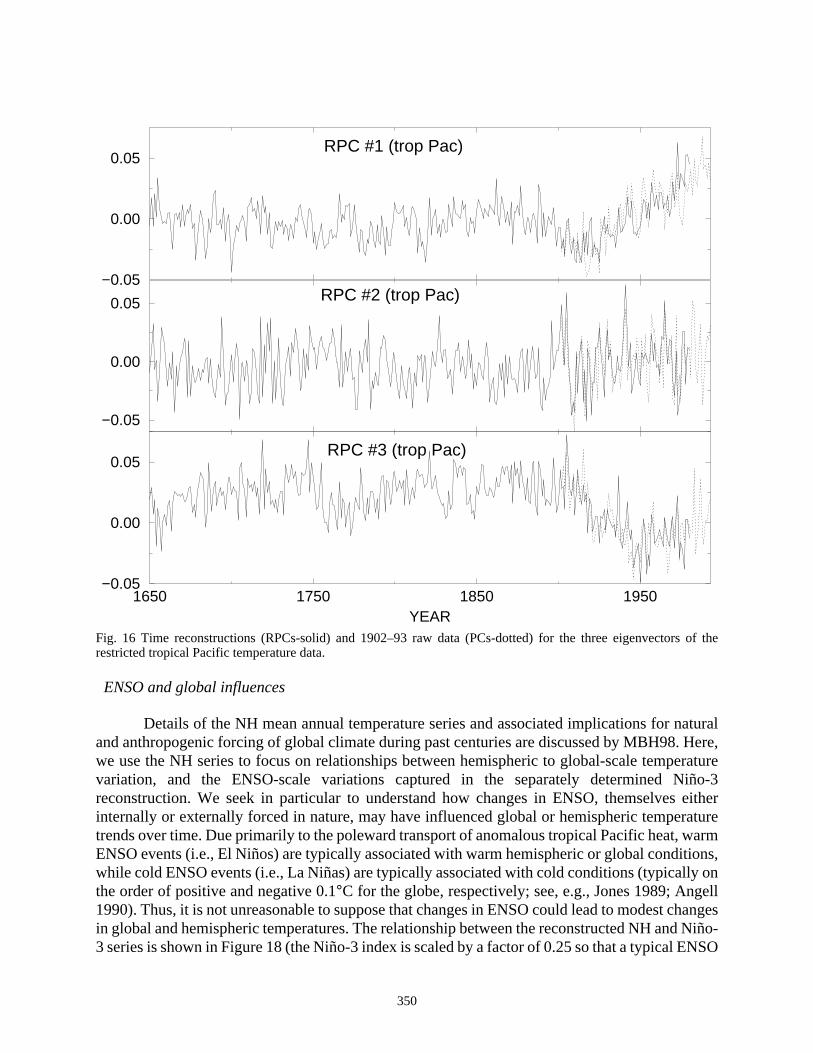
In Figure 16, we show the three RPCs corresponding to the separate tropical Preconstructions. As in the calibration interval (see Fig. 7), the interannual ENSO-related variaremains dominated by the RPC #2, while RPCs #1 and #3 describe in large part the anomtrends during the twentieth century in the region discussed earlier. The reconstructed Niño-3(Fig. 17) places recent large ENSO events in the context of a several centuries–long rallowing us to better gauge how unusual recent behavior might be. Indeed, the anomalous1983 El Niño event represents the largest positive event in our reconstructed chronology b1650. A similar statement holds for the current 1997/1998 event (not shown in Fig. 17), whof similar magnitude. Taking into account the uncertainties in the pre–twentieth-cenreconstructions, however, a more guarded statement is warranted. The 1982/1983 and 199events are both slightly greater than 2 standard errors (2s) warmer than any reconstructed, pevent. However, there are nine reconstructed events that are within 1.5-2.0 standard errors oof these two events. Roughly speaking, this lowers the probability to about 80% that eithertwo events in question is warmer thanany other single eventback to 1650, taking into account thcurrent uncertainties in the reconstruction. The significance of the occurrence of tworeasonablyunlikely events in the past 16 years, however, should clearly not be dismissed. Poindications of a recent change in the state of El Niño are discussed further in later sections

348

ectors.

Fig. 15 Time reconstructions (RPCs-solid) and 1902–93 raw data (PCs-dotted) for the first five global eigenv1902–80 calibration period means are indicated by the horizontal dotted lines.

1400 1500 1600 1700 1800 1900YEAR

−0.10

−0.05

0.00

0.05−0.10

−0.05

0.00

0.05−0.10

−0.05

0.00

0.05−0.10

−0.05

0.00

0.05−0.10

−0.05

0.00

0.05

RPC #1

RPC #2

RPC #3

RPC #4

RPC #5

349

of the

aturalHere,eratureiño-3either

aturearm

ions,y onellhangesNiño-NSO

Fig. 16 Time reconstructions (RPCs-solid) and 1902–93 raw data (PCs-dotted) for the three eigenvectorsrestricted tropical Pacific temperature data.

ENSO and global influences

Details of the NH mean annual temperature series and associated implications for nand anthropogenic forcing of global climate during past centuries are discussed by MBH98.we use the NH series to focus on relationships between hemispheric to global-scale tempvariation, and the ENSO-scale variations captured in the separately determined Nreconstruction. We seek in particular to understand how changes in ENSO, themselvesinternally or externally forced in nature, may have influenced global or hemispheric tempertrends over time. Due primarily to the poleward transport of anomalous tropical Pacific heat, wENSO events (i.e., El Niños) are typically associated with warm hemispheric or global conditwhile cold ENSO events (i.e., La Niñas) are typically associated with cold conditions (typicallthe order of positive and negative 0.1°C for the globe, respectively; see, e.g., Jones 1989; Ang1990). Thus, it is not unreasonable to suppose that changes in ENSO could lead to modest cin global and hemispheric temperatures. The relationship between the reconstructed NH and3 series is shown in Figure 18 (the Niño-3 index is scaled by a factor of 0.25 so that a typical E

1650 1750 1850 1950YEAR

−0.05

0.00

0.05

−0.05

0.00

0.05

−0.05

0.00

0.05RPC #1 (trop Pac)

RPC #2 (trop Pac)

RPC #3 (trop Pac)

350

not alatione twoges ints (seeveruringiño-3tieth1995;tures

uringenturylatterhole,ig. 7).nnual

tainedinstru-

event—e.g., a 0.5°C Niño-3 anomaly—is roughly in scale with an expected ~0.1°C NH meantemperature anomaly). Overall, the two series are modestly correlated (r = 0.14 for the 244-yearperiod 1650–1993, compared), which is significant at well above the 99% level whether orone-sided or two-sided significance test is used (one could argue that only a positive correshould be sought on physical grounds). However, the implied shared variance between thseries is less than 2%, which suggests that ENSO is not a dominant influence on chanhemispheric or global mean temperatures, at least in comparison with external forcing agenMBH98). Both Niño-3 and NH do show similar low-frequency variations at times, howe(compare the 50-year smoothed curves in Fig. 18), with warming occurring in both cases dthe seventeenth/early eighteenth, and twentieth centuries. The low-frequency variations in Nare nonetheless relatively muted compared to those in NH, particularly during the twencentury, when NH warming appears to become dominated by greenhouse forcing (IPCCMBH98). In contrast to the NH series, there is no evidence of any significant long-term deparfrom the twentieth-century climatology (see Fig. 17). There are in fact notable periods dwhich the low-frequency trends are uncorrelated or even opposite (e.g., late eighteenth cthrough mid-nineteenth century). It is interesting, though perhaps coincidental, that thisperiod corresponds to an anomalously cool period for the Northern Hemisphere on the wassociated with low solar irradiance, and preceding any greenhouse warming (see MBH98, FAs is discussed in later sections, this is also a period of anomalously weak amplitude interavariability in ENSO, and unusual global patterns of ENSO temperature influence.

Fig. 17 Reconstructed Niño-3 index back to 1650, along with instrumental series from 1902–93. The region conby the positive and negative 2 standard uncertainty limits in the reconstruction is shown (shaded) prior to themental calibration period. The calibration period (1902–80) mean is shown by the horizontal dashed line.

1650 1750 1850 1950YEAR

−1.5

−1.0

−0.5

0.0

0.5

1.0

1.5

TE

MP

ER

AT

UR

E A

NO

MA

LY

(oC

)

ANNUAL NINO3 INDEX

reconstruction (1650−1980)raw data (1902−1993)calibration period (1902−1980) mean

351

3 index

cans alsock topparentmorewhat

re is,ecentelayedtionsimplelong-on our

ENSO

ce ofNSOed by

are

Fig. 18 Comparison of reconstructed Northern Hemisphere (NH) mean annual temperature series and Niño-(rescaled by a factor of 0.25) from 1650–1980, along with 50-year smoothed versions of each series.

The muted positive trend in Niño-3 relative to that in NH during the twentieth centurybe attributed to the negative twentieth-century trend in eigenvector #2 noted earlier. As wadiscussed earlier, this offsetting trend might in turn be related to the negative feedbagreenhouse warming discussed by Cane et al. (1997). On the other hand, there is a strong arelationship between global temperature increases and warm ENSO conditions during thebrief period of the past couple decades (e.g., Trenberth 1990), and this period coincides withappear to be the warmest hemispheric conditions of the past six centuries (MBH98). Thefurthermore, evidence of distinct and unusual dynamical behavior of ENSO during this most rperiod. For example, Goddard and Graham (1998) argue for a breakdown of the classical doscillator mechanism in describing the vertical oceanographic evolution of ENSO-like variaduring the 1990s. Interdecadal ENSO-like variability (as discussed below) complicates any sinterpretation of trends in ENSO during the most recent decades, however. Thus, while theterm relationships between ENSO and global temperature changes appear modest basedreconstructions, the possible relationships between recent global warming and changes inare not yet clearly resolved.

Stationarity of ENSO teleconnections

It is also of interest to estimate the changes over time in the global pattern of influenENSO (i.e., the “teleconnections” of ENSO). Figure 11 showed that the modern global Epattern—as described through the global correlation map of the Niño-3 index—is well capturour multiproxy calibrations. Though the global patterns of ENSO in our reconstructions

1650 1750 1850 1950−0.5

−0.3

−0.1

0.1

0.3

NINO3 vs NH

NHNINO3

352

atureslobalile thethat

identlater

lationions inppearshoe”

entralure oforth

d keep. ThectionNSO-ity inby all

atternand

torialm aernalern, aobustnualSOnse to

e notENSOMann

described by a limited number of distinct global patterns or degrees of freedom, and not all feare expected to be well described given the variable spatial reconstructive skill of the greconstructions (e.g., parts of the southeastern United States; see Fig. 12). However, whdetails of different ENSO events may be described only approximately, it is certainly truedifferent “flavors” of the global ENSO phenomenon are reasonably well described. This is evin the reconstructions of global temperature patterns for specific ENSO years shown in asection.

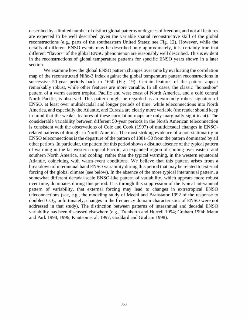
We examine how the global ENSO pattern changes over time by evaluating the corremap of the reconstructed Niño-3 index against the global temperature pattern reconstructsuccessive 50-year periods back to 1650 (Fig. 19). Certain features of the pattern aremarkably robust, while other features are more variable. In all cases, the classic “horsepattern of a warm eastern tropical Pacific and west coast of North America, and a cold cNorth Pacific, is observed. This pattern might be regarded as an extremely robust signatENSO, at least over multidecadal and longer periods of time, while teleconnections into NAmerica, and especially the Atlantic, and Eurasia are clearly more variable (the reader shoulin mind that the weaker features of these correlation maps are only marginally significant)considerable variability between different 50-year periods in the North American teleconneis consistent with the observations of Cole and Cook (1997) of multidecadal changes in Erelated patterns of drought in North America. The most striking evidence of a non-stationarENSO teleconnections is the departure of the pattern of 1801–50 from the pattern dominatedother periods. In particular, the pattern for this period shows a distinct absence of the typical pof warming in the far western tropical Pacific, an expanded region of cooling over easternsouthern North America, and cooling, rather than the typical warming, in the western equaAtlantic, coinciding with warm-event conditions. We believe that this pattern arises frobreakdown of interannual band ENSO variability during this period that may be related to extforcing of the global climate (see below). In the absence of the more typical interannual pattsomewhat different decadal-scale ENSO-like pattern of variability, which appears more rover time, dominates during this period. It is through this suppression of the typical interanpattern of variability, that external forcing may lead to changes in extratropical ENteleconnections (see, e.g., the modeling study of Meehl and Branstator 1992 of the respodoubled CO2; unfortunately, changes in the frequency domain characteristics of ENSO weraddressed in that study). The distinction between patterns of interannual and decadalvariability has been discussed elsewhere (e.g., Trenberth and Hurrell 1994; Graham 1994;and Park 1994, 1996; Knutson et al. 1997; Goddard and Graham 1998).

353

lor scalegraynd red

Fig. 19 Niño-3 temperature correlation map in successive 50-year periods between 1650 and present. The coshown indicates the specific level of correlation with a given grid point, with any color value outside of thecategory indicating significance at greater than a 70% level (based on a two-sided test), and with blue aindicating significance at well above the 99% level.

354

s (see.

Fig. 20 Evolutive spectrum of Niño-3 index (top) and evolutive multivariate spectrum of global temperature fieldtext for methodological details) for the period 1650–1980, employing an 80-year moving window through time

1700 1800 1900

0.4

0.3

0.2

0.1

0.0

YEAR

FREQUENCY (CYCLE/YR)

5.0 6.0

log spectrum

NINO3 SPECTRUM (EVOLUTIVE, 80 YR WINDOW)

1700 1800 1900

0.4

0.3

0.2

0.1

0.0

YEAR

FREQUENCY (CYCLE/YR)

0.7 0.8 0.9

LFV

MTM-SVD LFV SPECTRUM (EVOLUTIVE, 80 YR WINDOW)

355

istorylobaland itsossibleted in) and, welitude

ongerquencyof the; seeum ofarkes, wen in

ndow

thefor in1994;of thet of

abilityour

on, ofructedhe latecleariño-

n the

hle ettudethe

ith theing

idenceate.

ude oflobalrio islow-

CO

Frequency domain behavior

In this section, we investigate the frequency domain properties of the reconstructed hof ENSO and its large-scale teleconnections. A detailed study of the instrumental gtemperature record for changes in the frequency and amplitude characteristics of ENSOlarge-scale teleconnections has been recently undertaken by Park and Mann (1998). Pamplitude and frequency modulation of ENSO on longer timescales has been investigaprevious studies based on univariate (Michaelsen 1989; Meko 1992; Dunbar et al. 1994multivariate (Bradley et al. 1994) spectral analyses of ENSO-sensitive proxy data. Hereanalyze the reconstructions described in earlier sections to investigate low-frequency ampand frequency modulation of interannual variability, and the characteristics of decadal and ltimescale changes in the base state of ENSO. We analyze long-term changes in the fredomain aspects of El Niño and the global ENSO signal based on the evolutive spectrumreconstructed Niño-3 index (Fig. 20, top; calculated based on the “multitaper method”Thomson 1982; Park et al. 1987; Mann and Lees 1996) and the evolutive multivariate spectrthe global temperature field (Fig. 20, bottom; based on the “MTM-SVD” method of Mann and P1996, 1998; see also Rajagopalan et al. 1998; Tourre et al. 1998), respectively. In both casemploy an 80-year moving window in time to investigate multidecadal amplitude modulatioENSO and its global teleconnections. Similar results are obtained for 50- or 100-year wichoices.

A general tendency towards relatively higher-frequency interannual variability duringpast few centuries (e.g., from 5- to 7-year period, to 4- to 5-year period) has been arguedprevious proxy ENSO studies (e.g., Dunbar et al. 1994; Michaelsen 1989; Diaz and PulwartyKnutson et al. 1997). Such a trend is, arguably, evident in the evolutive spectral analysisNiño-3 index (Fig. 20, top). Frequency modulation of ENSO is not necessarily a fingerprinanthropogenic climate change (see Knutson et al. 1997) and is consistent with natural variin models of ENSO (Zebiak and Cane 1991; Knutson et al. 1997). What is more striking inanalysis, however, is not the frequency modulation, but rather the strong amplitude modulatithe variability. There is evidence for relatively enhanced interdecadal variance in the reconstNiño-3 series during the twentieth century, and relatively enhanced secular variance during teighteenth century (Fig 20). The most pronounced amplitude modulation, however, is thebreakdown in interannual variability during the early and mid-nineteenth century in both the N3 index (Fig. 20, top) and the global temperature field (Fig. 20, bottom). This latter behavior iNiño-3 index is consistent with the evolutive spectral analysis of the Galapagos coral d18O record(Dunbar et al. 1994) and time series waveform decompositions of SOI reconstructions (Staal. 1998), both of which show weakened interannual variability during this period. This amplimodulation is intriguing from the standpoint of possible external forcing. This period is alsocoldest during the interval examined here in terms of NH mean temperature, associated w“Maunder Minimum” period of relatively low apparent levels of solar irradiance, and precedthe marked twentieth-century greenhouse gas increases (see MBH98, Fig. 7). This coincsuggests the possibility that interannual ENSO variability is a feature of a relatively warm climIf this is the case, we might expect accelerated greenhouse forcing to increase the amplitinterannual ENSO variability. On the other hand, there may also be an upper limit on the gtemperature regime within which interannual ENSO variability can reside. The latter scenahinted at by the experiments of Knutson et al. (1997), which explored the response of aresolution version of the Geophysical Fluid Dynamics Laboratory (GFDL) coupled model to2

356

n an—e.g.,rmore,

ppears.tureienniale, e.g.,-yearssed1994,3 andbeensed ineratedNiño-s be

f thepicalobal1996;tivelybothcificg thetlanticopical) havel dataddard995),.

forcing, and showed a decrease in the amplitude of interannual ENSO-like variability ienhanced greenhouse climate (Knutson et al. 1997. We note, however, that other modelsZebiak and Cane 1991; Meehl and Branstator 1992—do not show such a response). FurtheGoddard and Graham (1998) point out that the interannual delayed oscillatory mechanism ato have broken down in describing the more trendlike ENSO-related variability of the 1990s

The primary differences between the evolutive Niño-3 and multivariate global temperaspectra (Fig. 20) are at the quasi-biennial and decadal-to-secular frequencies. The quasi-bsignal appears to be associated with extratropical features largely unrelated to ENSO (seMann and Park 1994, 1996), while the multidecadal (secular within the context of an 80window) global variations are associated with the North Atlantic multidecadal pattern discuearlier (see, e.g., Delworth et al. 1993, 1997; Kushnir 1994; Mann et al. 1995; Mann and Park1996). The interdecadal (15–30) year signal which intermittently appears in both the Niño-global multivariate spectra is associated with interdecadal ENSO-like variability that hasestablished in previous analyses of multiproxy data (Mann et al. 1995), and which is discusmore detail below. As was noted earlier, the reconstructed Niño-3 index has slightly exaggpower at decadal and lower frequencies in the twentieth century, relative to the instrumental3 index (see Fig. 10). The amplitude of decadal, relative to interannual, power may thusomewhat exaggerated in the reconstructed Niño-3 index.

To illustrate the fundamental differences referred to earlier in the spatial pattern ointerannual (“true”) ENSO signal, and the decadal ENSO-like signal, we reconstruct a tyoscillatory episode of the roughly 4- to 5-year (Fig. 21) and roughly 20- to 25-year (Fig. 22) gltemperature signals based on the MTM-SVD method described by Mann and Park (1994;1998). The primary departure of the interdecadal pattern from the ENSO pattern is the relasubdued amplitude in the tropical Pacific, and a cooling (rather than warming) influence overthe North American and tropical Atlantic sectors coincident with warm eastern tropical Pa(i.e., El Niño) conditions. The relative prominence of the decadal-scale ENSO pattern durinearly nineteenth century thus appears to explain the unusual Pacific North American and Ateleconnection pattern commented on earlier (Fig. 19). Possible origins and extratropical-trconnections that may describe the decadal signal (and its possible relationship with ENSObeen widely discussed elsewhere based on analyses of twentieth-century instrumenta(Trenberth 1990; Graham 1994; Trenberth and Hurrell 1994; Mann and Park 1994, 1996; Goand Graham 1998; Park and Mann 1998), long-term proxy climate indicators (Mann et al. 1and modeling experiments (Latif and Barnett 1994; Graham 1994; Gu and Philander 1997)

357

r half of

Fig. 21 Canonical pattern of the interannual ENSO signal in the temperature reconstructions as it evolves ovea typical (roughly 4-year period) cycle.

t=0

t=0.5 yr

t=1 yr

t=1.5 yr

t=2 yr

358

es overcorre-

Fig. 22 Canonical pattern of the interdecadal ENSO-like signal in the temperature reconstructions as it evolvhalf of a typical cycle. The cycle length is variable from about a16- to 25-year period, with the case shownsponding to the dominant roughly 25-year period evident during the early nineteenth century.

t=0

t=3 yr

t=6 yr

t=9 yr

t=12 yr

359

iñoses ofarianceiño-3in Fig.

d-orderdow)r thanof thelous

lity of

andfrom the

mid-arm

nnualtime.teenthbutionticallyand

duringach atutionts (see,

inHoar

whichnusualre 24pted

maticthisasesspelluch aswarmy an

forearly

ted, asparent

Trends in extremes

We can further quantify variations in the rates of extreme events (e.g., both large El Nand La Niñas) commented upon earlier, by looking at how frequencies of occurrencanomalous events have changed over time in our Niño-3 reconstructions. Because the vproperties appear to be homogeneous back in time (the resolved variance in our Nreconstructions is a roughly constant ~40% back in time; see Table 3, and also the error bars17), we consider it reasonable to examine the changes in the distribution—at least the seconstatistics—back in time. Figure 23 shows the variations over time (in an 80-year moving winin the frequency of anomalous cold and warm events (defined by an event amplitude greateone standard deviation, based on the calibration period [1902–80] mean and varianceinstrumental Niño-3 index). The low-frequency variations in the frequency of both anomawarm and cold events are similar to estimates of the low-frequency variations in the probabiall (weak and strong) warm events based on combined documentary, tropical ice core d18O, andextratropical dendroclimatic-based indices of ENSO-related variability (MichaelsenThompson 1992). In each case, a pronounced decreasing trend in occurrences is observedeighteenth through mid-nineteenth century, and a pronounced increasing trend from thenineteenth through early twentieth century. The unusually low incidence of anomalous wevents during the early nineteenth century, coincides closely with the breakdown of interavariability (Fig. 20), and altered global teleconnection patterns (Fig. 19) during that period ofAside from the overall trend of increases in both cold and warm extremes since the mid-ninecentury, our analysis indicates a trend towards enhanced skewness of the Niño-3 distriduring the twentieth century. The frequency of anomalous cold events has increased dramaduring the twentieth century, similar to the warm event occurrence rates of MichaelsenThompson (1992), while the frequency of anomalous warm events has actually decreasedthe early twentieth century. Cold and warm event occurrences, otherwise, largely track emultidecadal and longer timescales. It is interesting that this skewness of the Niño-3 distribappears to be reversing in recent decades, owing to the recent run of anomalous warm evene.g., Trenberth 1990).

The possibility that El Niño episode durations or “spell lengths” have increasedassociation with global warming has been highlighted by the recent study of Trenberth and(1996; see also the follow-ups by Rajagopalan et al. 1997; Trenberth and Hoar 1997),emphasized the unusually long nature of the 1990–95 warm episode. We investigate how usuch a warm spell is within the context of our several centuries–long reconstructions. Figushows the frequency of 5-year-long “warm spells,” defined as the number of distinct, uninterrustretches of positive Niño-3 values per 80-year period, as a function of time. The most drafeature is the trend towards far fewer long “warm spells” during the twentieth century. Incontext, the 1990–95 event is particularly striking, occurring during the period of recent increin warm event frequencies (Fig. 23) and anomalous warm events (Fig. 17). However, thisdoes not appear especially unusual when viewed in the context of certain previous periods, sthe early nineteenth century, during which there were between three and five 5-year-longevents within the confines of our estimated uncertainties. This finding is supported bindependent proxy-based study by Allan and D'Arrigo (1998), which provides evidencenumerous “persistent” warm episodes in past centuries. It is worth emphasizing that thenineteenth-century period associated with the greatest probability of warm spells is associawas commented upon earlier, with the coldest global temperatures back to 1650, and an ap

360

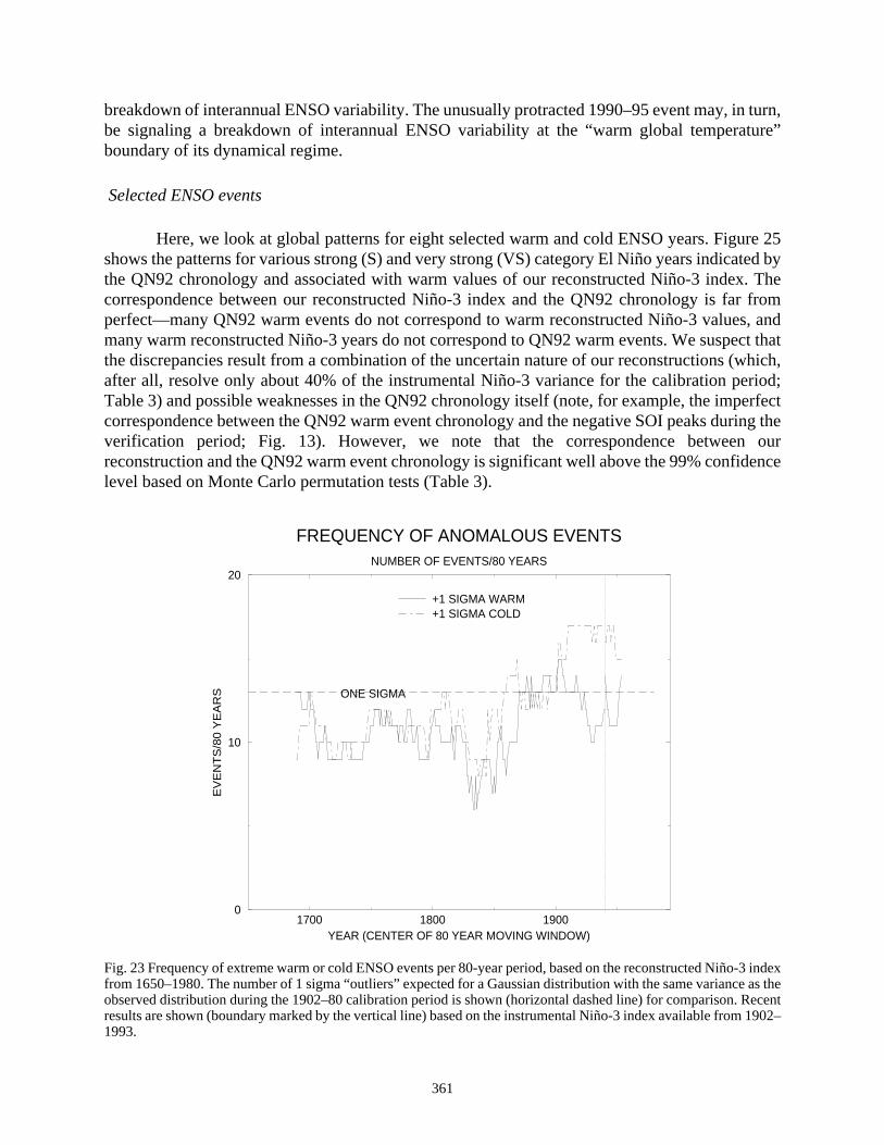
turn,ure”

re 25ted by. Ther froms, andct thathich,

riod;erfectring the

ourence

-3 indexas theecent1902–

breakdown of interannual ENSO variability. The unusually protracted 1990–95 event may, inbe signaling a breakdown of interannual ENSO variability at the “warm global temperatboundary of its dynamical regime.

Selected ENSO events

Here, we look at global patterns for eight selected warm and cold ENSO years. Figushows the patterns for various strong (S) and very strong (VS) category El Niño years indicathe QN92 chronology and associated with warm values of our reconstructed Niño-3 indexcorrespondence between our reconstructed Niño-3 index and the QN92 chronology is faperfect—many QN92 warm events do not correspond to warm reconstructed Niño-3 valuemany warm reconstructed Niño-3 years do not correspond to QN92 warm events. We suspethe discrepancies result from a combination of the uncertain nature of our reconstructions (wafter all, resolve only about 40% of the instrumental Niño-3 variance for the calibration peTable 3) and possible weaknesses in the QN92 chronology itself (note, for example, the impcorrespondence between the QN92 warm event chronology and the negative SOI peaks duverification period; Fig. 13). However, we note that the correspondence betweenreconstruction and the QN92 warm event chronology is significant well above the 99% confidlevel based on Monte Carlo permutation tests (Table 3).

Fig. 23 Frequency of extreme warm or cold ENSO events per 80-year period, based on the reconstructed Niñofrom 1650–1980. The number of 1 sigma “outliers” expected for a Gaussian distribution with the same varianceobserved distribution during the 1902–80 calibration period is shown (horizontal dashed line) for comparison. Rresults are shown (boundary marked by the vertical line) based on the instrumental Niño-3 index available from1993.

1700 1800 1900YEAR (CENTER OF 80 YEAR MOVING WINDOW)

0

10

20

EV

EN

TS

/80

YE

AR

S

FREQUENCY OF ANOMALOUS EVENTSNUMBER OF EVENTS/80 YEARS

+1 SIGMA WARM+1 SIGMA COLD

ONE SIGMA

361

iño-33 index

spellsuncer-

ing toarmandrgelys of theof then, isacificrn. Inbably

cessesr time

Fig. 24 Frequency of unusually (5-year) long warm ENSO “spells” per 80-year period, for the reconstructed Nindex from 1650–1980 (solid curve). Recent results are shown (dotted curve) based on the instrumental Niño-available from 1902–93; 1 standard uncertainty limits are indicated (dashed) for the estimated number of warmin a given 80-year period. These limits were determined from Monte Carlo simulations taking into account thetainties in the Niño-3 reconstruction itself (see Fig. 17).

The pattern for 1652 (shown, as in all events, relative to a zero reference correspondthe 1902–80 climatology) indicates warming in the Niño-3 region, but an unusual lack of wanomalies along Pacific coastal South and Central America. This is similarly true for 18041828, which show cooling or neutral anomalies in most areas other than the Niño-3 region, labecause these events are superimposed on the considerably cold global baseline conditionearly nineteenth century discussed earlier. The 1828 pattern, which also falls in the center1801–50 period earlier noted (Fig. 19) for its unusual global ENSO correlation patterparticularly atypical. The 1877 and 1884 events exhibit particularly strong tropical eastern Pwarm tongue anomalies, which are more typical of the twentieth century (e.g., Fig. 11) pattesummary, the patterns of different reconstructed ENSO years are quite variable—this is produe in part to the inherent event-to-event noise, in part to the obscuring influence of other proinfluencing global temperatures, and in part to real changes in ENSO teleconnections ove(e.g., Fig. 19).

1650 1750 1850 1950YEAR (CENTER OF 80 YEAR WINDOW)

0

2

4

NU

MB

ER

OF

5−

YE

AR

WA

RM

SP

EL

LS

NINO3 WARM SPELLS# of 5−year long events in an 80 year period

RECONSTRUCTED NINO3RAW (INSTRUMENTAL) NINO3

362

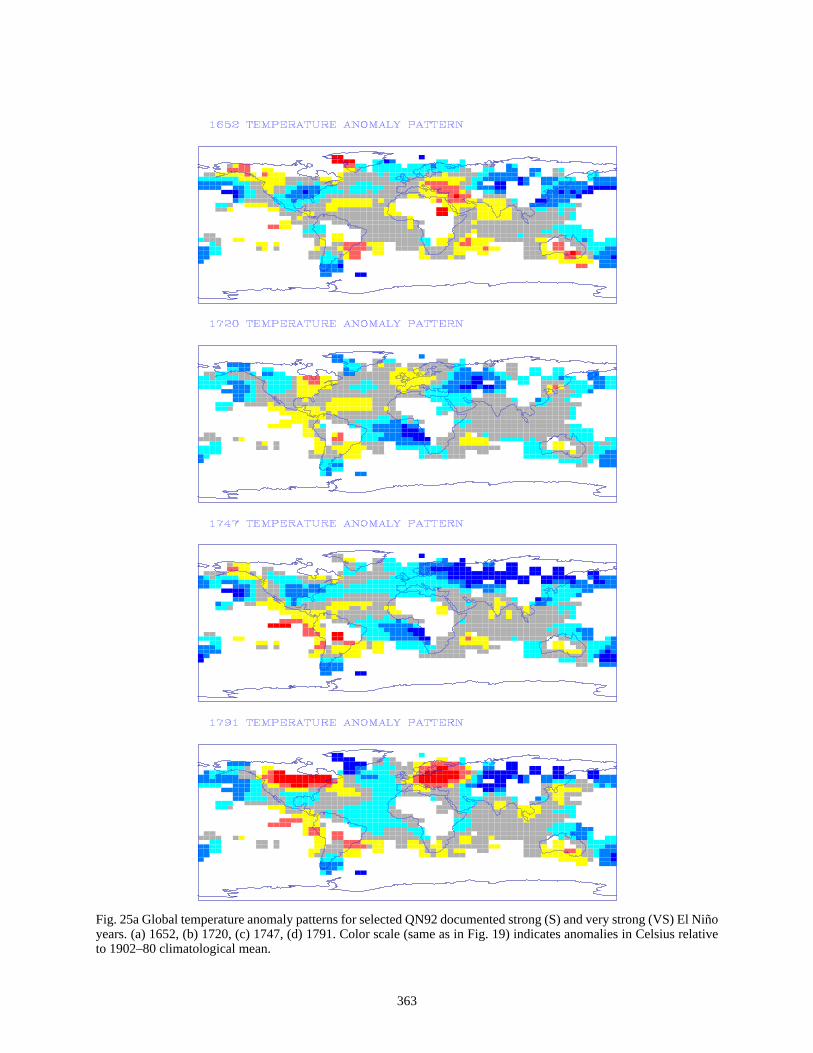
El Niñorelative

Fig. 25a Global temperature anomaly patterns for selected QN92 documented strong (S) and very strong (VS)years. (a) 1652, (b) 1720, (c) 1747, (d) 1791. Color scale (same as in Fig. 19) indicates anomalies in Celsiusto 1902–80 climatological mean.

363

El Niñorelative

Fig. 25a Global temperature anomaly patterns for selected QN92 documented strong (S) and very strong (VS)years. (a) 1804, (b) 1828, (c) 1877, (d) 1884. Color scale (same as in Fig. 19) indicates anomalies in Celsiusto 1902–80 climatological mean.

364

uringwarmperiod.tury

ttedricaliña,, and

d coldnturyight

nce, itstrong

1777.

Figure 26 shows global temperature anomaly patterns for two selected cold events dthe eighteenth century. Note that the patterns depart significantly from the mirror images ofevents such as are shown in Figure 25, in large part because of the colder climatology of theFor example, neutral conditions in the central North Pacific relative to the twentieth-cenclimatology would actually correspond to more familiar warm conditions in the region if plorelative to the colder eighteenth-century climatology. There is no independent histocorroboration of cold events, as the QN92 index documents only El Niño, and not La Nepisodes. The cold events typically, as we would expect, fall between QN92 warm eventsfrequently right after warm events. For example, the notable 1732 and 1777 reconstructeevents shortly follow the 1728 VS and 1775 S warm events, respectively. The eighteenth cewas a time of relatively pronounced interannual variability in Niño-3 (see Fig. 20), so we mtend to believe that the delayed oscillator mechanism was particularly active at this time. Heis reasonable to conclude that strong warm events should tend to be followed by particularlycold events during this period.

Fig. 26 Global temperature anomaly patterns for two reconstructed cold ENSO (La Niña) years. (i) 1732, (ii)Conventions are as in Figure 25.

365

enceng itsnturyas areenictrendsds ing theks may

litudeand

to haveeased.recentars to

ectiondownglobalO ands of

omele with

e thec toNSO

1990–e, weepresent

Alanerousin this

arence.ergy.

ctoralto the

Conclusions

The multiproxy-based reconstructions of El Niño and its large-scale patterns of infludescribed in this chapter provide insight into a number of issues related to ENSO, includinatural variability, and varying large-scale teleconnections on multidecadal and cetimescales. Relationships with global or hemispheric mean temperatures are also evident,possible relationships with natural and external forcing of climate, including anthropogfactors. Certain ENSO-related patterns and features appear to have exhibited significantduring the twentieth century, although classic ENSO indices show only modest warming trencomparison with the dramatic warming trend in hemispheric and global temperature durinpast century. There is some evidence that a pattern associated with negative tropical feedbacbe abating an El Niño–like warming trend in the tropical Pacific.

Equally interesting in the climate reconstructions is evidence of changes in the ampof interannual ENSO variability, global teleconnections of ENSO, and the amplitudefrequency of extremes. For example, the incidence of large warm and cold events appearsincreased during the past century, while the frequency of long warm ENSO spells has decrThere is evidence, however, that some of these trends may be reversing during the mostdecades. The breakdown of interannual ENSO variability during the nineteenth century appehave had particularly significant impacts on the incidence of extremes and on global teleconnpatterns of ENSO during that period. We find some support for the proposition that this breakmay have been associated with the same external forcings that led to generally coldtemperatures at the time. This period may thus provide an analog for the behavior of ENSthe possible breakdown of typical mechanisms of ENSO variability under the impactexternal—including anthropogenic—forcing of climate.

As increasingly rich networks of high-quality, seasonally resolved proxy data becavailable, both global temperature pattern and ENSO-scale reconstructions should be possibconsiderably reduced uncertainties. Of particular utility for ENSO-scale reconstruction will bavailability of a greater number of well-dated coral isotopic indicators in the tropical Pacifisupplement the sparse existing network. With reduced uncertainties, indices of past Evariability should allow the unusual 1982/1983 and 1997/1998 warm events, and protracted95 “warm spell” to be placed in a proper longer-term perspective. With such a perspectivshould be better able to assess whether or not these seemingly anomalous recent events rsignificant and potentially anthropogenic-related climate changes.

Acknowledgments

We are indebted to Rosanne D'Arrigo, David Fisher, Gordon Jacoby, Judith Lean,Robock, David Stahle, Charles Stockton, Eugene Vaganov, Ricardo Villalba, and the numcontributors to the International Tree-Ring Data Bank for many of the proxy data series usedstudy. We thank Mike Dettinger for a thoughtful and thorough review of the manuscript. Wealso grateful to Frank Keimig, Martin Munro, and Richard Holmes for their technical assistaThis work was supported by the National Science Foundation and the Department of EnM.E.M. acknowledges support through the Alexander Hollaender Distinguished PostdoResearch Fellowship program of the U.S. Department of Energy. This work is a contribution

366

ional

990–

iño

atural

low-

?,

nature

bility

short

s of

usual

s in El

rom

hern

t over

Analysis of Rapid and Recent Climatic Change (ARRCC) project, sponsored by the NatScience Foundation and the U.S. National Oceanic and Atmospheric Administration.

References

Allan, R., and D'Arrigo, R.D., 1998: “Persistent” ENSO sequences: How unusual was the 11995 El Niño?Holocene, in press.

Allan, R., Lindesay, J., and Parker, D., 1996:El Niño Southern Oscillation and ClimateVariability. CSIRO Publishing, Melbourne.

Angell, J.K., 1990: Variation in global tropospheric temperature after adjustment for the El Ninfluence, 1958–1989.Geophysical Research Letters, 17, 1093–1096.

Barnett, T.P., Santer, B., Jones, P.D., and Bradley, R.S., 1996: Estimates of low frequency nvariability in near-surface air temperature.Holocene, 6, 255–263.

Barnston, A.G., and Livezey, R.E., 1987: Classification, seasonality and persistence offrequency atmospheric circulation patterns.Monthly Weather Review, 115, 1083–1126.

Boninsegna, J.A., 1992: South American dendroclimatological records.In: Climate Since A.D.1500,Bradley, R.S., and Jones, P.D. (eds.), Routledge, 246–268.

Bradley, R.S., 1996: Are there optimum sites for global paleotemperature reconstructionIn:Climatic Variations and Forcing Mechanisms of the Last 2000 Years,Jones, P.D., Bradley, R.S.and Jouzel, J. (eds.), Springer-Verlag, 603–624.

Bradley, R.S., and Jones, P.D., 1993: 'Little Ice Age' summer temperature variations: Theirand relevance to recent global warming trends.Holocene, 3, 367–376.

Bradley, R.S., Mann, M.E., and Park, J., 1994: A spatiotemporal analysis of ENSO variabased on globally distributed instrumental and proxy temperature data.EOS Supplement, 75,383.

Briffa, K.R., et al., 1992a: Fennoscandian summers from AD 500: Temperature changes onand long timescales.Climate Dynamics, 7, 111–119.

Briffa, K.R., Jones, P.D., Schweingruber, F.H., 1992b: Tree-ring density reconstructionsummer temperature patterns across western North America since 1600.Journal of Climate, 5,735–753.

Briffa, K.R., Jones, P.D., Schweingruber, F.H., Shiyatov, S.G., and Cook, E.R., 1995: Untwentieth-century summer warmth in a 1000-year temperature record from Siberia.Nature, 376,156–159.

Cane, M., et al., 1997: Twentieth-century sea surface temperature trends.Science, 275, 957–960.Chang, P., Ji, L., Li, H., and Flugel, M., 1996: Chaotic dynamics versus stochastic processe

Niño–Southern Oscillation in coupled ocean-atmosphere models.Physica D., 98, 301–320.Chang, P., Ji, L., and Li, H., 1997: A decadal climate variation in the tropical Atlantic Ocean f

thermodynamic air-sea interactions.Nature, 385, 516–518.Cleaveland, M.K., Cook, E.R., and Stahle, D.W., 1992: Secular variability of the Sout

Oscillation detected in tree-ring data from Mexico and the southern United States.In: El Niño:Historical and Paleoclimatic Aspects of the Southern Oscillation, Diaz, H.F., and Markgraf, V.(eds.), Cambridge University Press, Cambridge, 271–291.

Cole, J., and Cook, E., 1997: The coupling between ENSO and U.S. drought: How stable is ithe past century?EOSSupplement, 78.

367

ation:

-ring

logy:

ent

face

the

aline

the

rn

long

seas

fromn detailrs,

Foxe

tions

.

s fors in

970s

Cole, J.E., Fairbanks, R.G., and Shen, G.T., 1993: Recent variability in the Southern OscillIsotopic results from a Tarawa atoll coral.Science, 260, 1790–1793.

Cook, E.R., et al., 1991: Climatic change in Tasmania inferred from a 1089-year treechronology of Huon pine.Science, 253, 1266–1268.

Cook, E.R., Briffa, K.R., and Jones, P.D., 1994: Spatial regression methods in dendroclimatoA review and comparison of two techniques.International Journal of Climatology, 14, 379–402.

Cook, E.R., Briffa, K.R., Meko, D.M., Graybill, D.A., and Funkhouser, G., 1995: The 'segmlength' curse in long tree-ring chronology development for paleoclimatic studies.Holocene, 5,229–237.

D'Arrigo, R.D., Cook, E.R., Jacoby, G.C., and Briffa, K.R., 1993: NAO and sea surtemperature signatures in tree-ring records from the North Atlantic sector.Quaternary ScienceReview, 12, 431–440.

Delworth, T.D., and Mann, M.E., 1998: Observed and Simulated Multidecadal Variability inNorth Atlantic. (Submitted).

Delworth, T.D., Manabe, S., and Stouffer, R.J., 1993: Interdecadal variations of the thermohcirculation in a coupled ocean-atmosphere model.Journal of Climate, 6, 1993–2011.

Delworth, T.D., Manabe, S., and Stouffer, R.J., 1997: Multidecadal climate variability inGreenland Sea and surrounding regions: A coupled model simulation.Geophysical ResearchLetters, 24, 257–260.

Diaz, H.F., and Markgraf, V., 1993:El Niño: Historical and Paleoclimatic Aspects of the SoutheOscillation.Cambridge University Press, Cambridge, 476pp.

Diaz, H.F., and Pulwarty, R.S., 1994: An analysis of the time scales of variability in centuries-ENSO-sensitive records in the last 1000 years.Climatic Change, 26, 317–342.

Dunbar, R.B., Wellington, G.M., Colgan, M.W., and Glynn, P.W., 1994: Eastern Pacificsurface temperature since 1600 A.D. The d18O record of climate variability in the Galapagocorals.Paleoceanography, 9, 291–315.

Fisher, D.A., et al., 1996: Inter-comparison of ice core delta O-18 and precipitation recordssites in Canada and Greenland over the last 3500 years and over the last few centuries iusing EOF techniques.In: Climatic Variations and Forcing Mechanisms of the Last 2000 YeaJones, P.D., Bradley, R.S., and Jouzel, J., Springer-Verlag, Heidelberg, 297–328.

Fisher, D.A., et al., 1998: Penny ice cap cores, Baffin Island, Canada, and the WisconsinDome connection: Two states of Hudson Bay ice cover.Science, 279, 692–965.

Folland, C.K., Parker, D.E., and Kates, F.E., 1984: Worldwide marine temperature fluctua1856–1981.Nature, 310, 670–673.

Fritts, H., 1991:Reconstructing Large-Scale Climatic Patterns from Tree Ring Data, Universityof Arizona Press Tucson.

Fritts, H.C., and Shao, X.-M., 1992:In: Climate Since A.D. 1500, Bradley, R.S., and Jones, P.D(eds.), Routledge, 269–294.

Fritts, H.C., Blasing, T.J., Hayden, B.P., and Kutzbach, J.E., 1971: Multivariate techniquespecifying tree-growth and climate relationships and for reconstructing anomaliepaleoclimate.Journal of Applied Meteorology, 10, 845–864.

Goddard, L., and Graham, N.E., 1998: El Niño in the 1990s.Journal of Geophysical Research,102, 10423–10436.

Graham, N.E., 1994: Decadal-scale variability in the tropical and North Pacific during the 1and 1980s: Observations and model results.Climate Dynamics, 10, 135–162.

368

anges

ction

ith the

MAR

and

tieth-

and

f

rature

atic

ntury

onic

.

20

ean-

ciated

and

pical

Gu, D., and Philander, S.G.H., 1997: Interdecadal climate fluctuations that depend on exchbetween the tropics and extratropics.Science, 275, 805–807.

Guiot., J., 1988: The combination of historical documents and biological data in the reconstruof climate variations in space and time.Palaeoklimaforschung, 7, 93–104.

Halpert, M.S., and Ropelewski, C.F., 1992: Surface temperature patterns associated wSouthern Oscillation.Journal of Climate,5, 577–593.

Heiss, G.A., 1994: Coral reefs in the Red Sea: Growth, production and stable isotopes. GEOReport 32, 1–141.

Hughes, M.K., and Diaz, H.F., 1994: Was there a “Medieval Warm Period” and if so, wherewhen?Climatic Change, 26, 109–142.

Hughes, M.K., Vaganov, E.A., Shiyatov, S.A., Touchan, R., and Funkhouser, G., 1998: Twencentury summer warmth in northern Yakutia in a 600-year context. Submitted.

Hurrell, J.W., 1995: Decadal trends in the North Atlantic Oscillation, regional temperaturesprecipitation.Science, 269, 676–679.

Intergovernmental Panel on Climate Change (IPCC), 1995:Climate Change 1995: The Science oClimate Change,Houghton, J.T., et al. (eds.), Cambridge University Press, Cambridge.

Jacoby, G.C., and D'Arrigo, R., 1989: Reconstructed Northern Hemisphere annual tempesince 1671 based on high-latitude tree-ring data from North America.Climatic Change, 14, 39–59.

Jacoby, G.C., and D'Arrigo, R.D., 1990: Teak: A tropical species of large-scale dendroclimpotential.Dendrochronologia, 8, 83–98.

Jacoby, G.C., D'Arrigo, R.D., and Tsevegyn, D., 1996: Mongolian tree rings and 20th-cewarming.Science, 9, 771–773.

Jin, F.F, Neelin, J.D., and Ghil, M., 1994: El Niño on the devil's staircase: Annual subharmsteps to chaos.Science, 264, 70–72.

Jones, P.D., 1989: The influence of ENSO on global temperatures.Climate Monitor, 17, 80–89.Jones, P.D., 1998: It was the best of times, it was the worst of times.Science, 280, 544–545.Jones, P.D., and Bradley, R.S., 1992:In: Climate Since A.D. 1500,Bradley, R.S., and Jones, P.D

(eds.), Routledge, 246–268.Jones, P.D., and Briffa, K.R., 1992: Global surface air temperature variations during theth

century: Part I–Spatial, temporal and seasonal details.Holocene, 1, 165–179.Kameda, T., Narita, H., Shoji, J., Nishio, F., and Watanabe, O., 1992:Proc. International

Symposium on the Little Ice Age Climate,Tokyo Metropolitan University, Tokyo, Japan.Kaplan, A., et al., 1998: Analyses of global sea surface temperature 1856–1991.Journal of

Geophysical Research,in press.Knutson, T., Manabe, S., and Gu, D., 1997: Simulated ENSO in a global coupled oc

atmosphere model: Multidecadal amplitude modulation and CO2 sensitivity.Journal of Climate,10, 138–161.

Kushnir, Y., 1994: Interdecadal variations in North Atlantic sea surface temperature and assoatmospheric conditions.Journal of Climate, 7, 141–157.

Latif, M., and Barnett, T.P., 1994: Causes of decadal climate variability over the North PacificNorth America.Science, 266, 634–637.

Lau, N.C., and Nath, M.J., 1994: A modeling study of the relative roles of tropical and extratroSST anomalies in the variability of the global atmosphere-ocean system.Journal of Climate,7,1184–1207.

369

ith a

nter-

tion in

ty on

a level

es: A

ations

s and

uring.

tterns.

hernfss,

sed

ted torn375.uctedas,gton,

thern

Lau, N.C., Philander, S.G.H., and Nath, M.J., 1992: Simulation of ENSO-like phenomena wlow-resolution coupled GCM of the global ocean and atmosphere.Journal of Climate, 5, 284–307.

Linsley, B.K., Dunbar, R.B., and Mucciasone, D.A., 1994: A coral-based reconstruction of ITropical Convergence Zone variability over Central America since 1707.Journal of GeophysicalResearch, 99, 9977–9994.

Lough, J.M., 1991: Rainfall variations in Queensland, Australia: 1891–1986.InternationalJournal of Climatology, 11, 745–768.

Manley, G., 1959: Mean temperature of Central England 1698–1952.Quarterly Journal of theRoyal Meteorological Society, 79, 242–261.

Mann, M.E., and Lees, J., 1996: Robust estimation of background noise and signal detecclimatic time series.Climatic Change, 33, 409–445.

Mann, M.E., and Park, J., 1994: Global scale modes of surface temperature variabiliinterannual to century time scales.Journal of Geophysical Research, 99, 25819–25833.

Mann, M.E., and Park, J., 1996: Joint spatio-temporal modes of surface temperature and sepressure variability in the Northern Hemisphere during the last century.Journal of Climate, 9,2137–2162.

Mann, M.E., and Park, J., 1998: Oscillatory spatiotemporal signal detection in climate studimultiple-taper spectral domain approach.Advances in Geophysics, in press.

Mann, M.E., Park, J., and Bradley, R.S., 1995: Global interdecadal and century-scale oscillduring the past five centuries.Nature, 378, 266–270.

Mann, M.E., Bradley, R.S., and Hughes, M.K., 1998a: Global-scale temperature patternclimate forcing over the past six centuries.Nature, 392, 779–787.

Mann, M.E., Bradley, R.S., and Hughes, M.K., 1998b: Northern Hemisphere temperatures dthe past millennium: Inferences, uncertainties, and limitations.Geophysical Research LettersSubmitted.

Mann, M.E., Bradley, R.S., Hughes, M.K., and Jones, P.D., 1998c: Global temperature paScience, 280, 2029–2030.

Meehl, G.A., and Branstator, G.W., 1992: Coupled climate model simulation of El Niño/ SoutOscillation: Implications for paleoclimate.In: El Niño: Historical and Paleoclimatic Aspects othe Southern Oscillation, Diaz, H.F., and Markgraf, V. (eds.), Cambridge University PreCambridge, 69–91.

Meehl, G.A., and Washington, W.M., 1996: El Niño–like climate change in a model with increaatmospheric CO2 concentrations.Nature, 382, 56–60.

Meko, D., 1992: Spectral properties of tree-ring data in the United States Southwest as relaEl Niño/Southern Oscillation.In: El Niño: Historical and Paleoclimatic Aspects of the SoutheOscillation, Diaz, H.F., and Markgraf, V. (eds.), Cambridge Univ. Press, Cambridge, 349–

Michaelsen, J., 1989: Long-period fluctuations in El Niño amplitude and frequency reconstrfrom tree-rings.In: Aspects of Climate Variability in the Pacific and the Western AmericPeterson, D.H. (ed.), Geophysical Monograph 55, American Geophysical Union, WashinD.C., 69–74.

Michaelsen, J., and Thompson, L.G., 1992: A comparison of proxy records of El Niño/SouOscillation.In: El Niño: Historical and Paleoclimatic Aspects of the Southern Oscillation, Diaz,H.F., and Markgraf, V. (eds.), Cambridge University Press, Cambridge, 7–28.

Norton, D.A., and Palmer, J.G., 1992: Dendroclimatic evidence from Australasia.In: ClimateSince A.D. 1500,Bradley, R.S., and Jones, P.D. (eds.), Routledge, 463–482.

370

f the

rature:

igh-

979:

hy,

m a

tionNew

ative

h to

res in982.

eriod

l sea

tree

nges

.E.,ndtion.

from05–

the

Ortlieb, L., 1998: The documentary historical record of El Niño events in Peru: An update oQuinn record (sixteenth through nineteenth centuries), this volume.

Park, J., and Mann, M.E., 1998: Interannual temperature events and shifts in global tempeA multiple wavelet correlation approach.Earth Interactions, in revision.

Park, J., Lindberg, C.R., and Vernon, F.L., III, 1987: Multitaper spectral analysis of hfrequency seismograms.Journal of Geophysical Research, 92, 12675–12684.

Pfister, C., 1992: Monthly temperature and precipitation in central Europe from 1525–1quantifying documentary evidence on weather and its effects.In: Climate Since A.D. 1500,Bradley, R.S., and Jones, P.D. (eds.), Routledge, 118–142.

Philander, S.G.H., 1990:El Niño, La Niña, and the Southern Oscillation, Academic Press.Preisendorfer, R.W., 1988:Principal Component Analysis in Meteorology and Oceanograp

Elsevier, Amsterdam.Quinn, W.H., and Neal, V.T., 1992: The historical record of El Niño events.In: Climate Since A.D.

1500, Bradley, R.S., and Jones, P.D. (eds.), Routledge, 623–648.Quinn, T.M., Taylor, F.W., and Crowley, T.J., 1993: A 173 year stable isotope record fro

tropical South Pacific coral.Quaternay Science Reviews,12, 407–418.Quinn, T.M., Taylor, F.W., Crowley, T.J., and Link, S.M., 1996: Evaluation of sampling resolu

in coral stable isotope records: A case study using monthly stable isotope records fromCaledonia and Tarawa.Paleoceanography, 11, 529–542.

Rajagopalan, B., Lall, U., and Cane, M.A., 1997: Anomalous ENSO occurrences: An alternview. Journal of Climate, 10, 2351–2357.

Rajagopalan, B., Mann, M.E., and Lall, U., 1998: A multivariate frequency-domain approaclong-lead climatic forecasting.Weather and Forecasting, 13, 58–74.

Schweingruber, F.H., Briffa, K.R., and Jones, P.D., 1991: Yearly maps of summer temperatuwestern Europe from A.D. 1750 to 1975 and western North America from 1600 to 1Vegetatio, 92, 5–71.

Schlesinger, M.E., and Ramankutty, N., 1994: An oscillation in the global climate system of p65–70 years.Nature, 367, 723–726.

Smith, T.M., Reynolds, R.W., Livezey, R.E., Stokes, D.C., 1996: Reconstruction of historicasurface temperatures using empirical orthogonal functions.Journal of Climate, 9, 1403–1420.

Stahle, D.W., and Cleaveland, M.K., 1993: Southern Oscillation extremes reconstructed fromrings of the Sierra Madre Occidental and southern Great Plains.Journal of Climate, 6, 129–140.

Stahle, D.W., Cleaveland, M.K., and Heher, J.G., 1988: North Carolina climate chareconstructed from tree rings A.D. 372 to 1985.Science, 240, 1517–1519.

Stahle, D.W., D'Arrigo, R.D., Krusic, P.J., Cleaveland, M.K., Cook, E.R., Allan, R.J., Cole, JDunbar, R.B., Therell, M.D., Gay, D.A., Moore, M.D., Stokers, M.A., Burns, B.T., aThompson, L.G., 1998: Experimental dendroclimatic reconstruction of the Southern OscillaBulletin of the American Meteorological Society, submitted.

Tarussov, A., 1992: The Arctic and Svalbard to Severnaya Zemlya: climatic reconstructionsice cores.In: Climate Since A.D. 1500, Bradley, R.S., and Jones, P.D. (eds.), Routledge, 5516.

Thomson, D. J., 1982: Spectrum estimation and harmonic analysis.IEEE Proc.,70, 1055–1096.Thompson, L.G., 1992: Ice core evidence from Peru and China.In: Climate SinceA.D. 1500,

Bradley, R.S., and Jones, P.D. (eds.), Routledge, 517–548.Tourre, Y., Rajagopalan, B., and Kushnir, Y., 1998: Dominant patterns of climate variability in

Atlantic over the last 136 years.Journal of Climate, in press.

371

phere.

vent:

acific.

g of

and

Trenberth, K.E., 1990: Recent observed interdecadal climate changes in the Northern HemisBulletin of the Americal Meteorological Society, 71, 988–993.

Trenberth, K.E., and Hoar, T.J., 1996: The 1990–1995 El Niño–Southern Oscillation eLongest on record.Geophysical Research Letters, 23, 57–60.

Trenberth, K.E., and Hoar, T.J., 1997: El Niño and climate change.Geophysical Research Letters,24, 3057–3060.

Trenberth, K.E., and Hurrell, J.W., 1994: Decadal atmosphere-ocean variations in the PClimate Dynamics, 9, 303–319.

Tziperman, E., Stone, L., Cane, M.A., and Jarsoh, H., 1994: El Niño chaos: Overlappinresonances between the seasonal cycle and the Pacific ocean-atmosphere oscillator.Science, 264,72–74.

Zebiak, S.E., and Cane, M.A., 1987: A model El Niño–Southern Oscillation.Monthly WeatherReview, 115, 2262–2278.

Zebiak, S.E., and Cane, M.A., 1991: Natural climate variability in a coupled model.In:Greenhouse Gas–Induced Climatic Change: A Critical Appraisal of SimulationsObservations, Schlesinger, M.E. (ed.), Elsevier, 457–469.

372