long term structural design of geosynthetic … term structural design of geosynthetic stormwater...
TRANSCRIPT

Long Term Structural Design of Geosynthetic Stormwater Chambers
and the Use of Nanocompsites to Enhance Their Performance
A Thesis
Submitted to the Faculty
of
Drexel University
by
Archibald Stewart Filshill
in partial fulfillment of the
requirements for the degree
of
Doctor of Philosophy
June 2010

ii
© Copyright 2010
Archibald Stewart Filshill. All Rights Reserved.

iii
Dedication
To my family.
My parents Archie and Rose, for all of their support and encouragement.
My father for “pushing” me into engineering and my mother for her support throughout
school and constant reminding to enjoy myself during the process.
My wife Kelly and children Archie and Katie for all their loving support
and patience throughout this process and in all I do.
I am incredibly fortunate to have such a loving family.

iv
Acknowledgements
I would like to thank my advisor Dr. Joseph Martin whose
guidance, help and support throughout this process was invaluable.
To all my committee members, Dr. Shieh-Chi Cheng, Dr. Andrea Welker,
Dr. Morton Rabinowitz and Dr. Kurt Sjoblom for their help and support.
Dr Grace Hsuan for her technical support on this project.
Dr. Patricia Gallagher for her help throughout the process.
A very special thank you to the entire Koerner family.
For being such a supportive and positive influence in my life, personally, academically
and professionally, since we first met at Drexel
To John Henry for his friendship, advice and support on all of my projects.
Greg Hilley for all of his help and support during testing.

v
Table of Contents
LIST OF TABLES.......................................................................................................... ix
LIST OF ILLUSTRATIONS............................................................................................x
ABSTRACT.................................................................................................................. xiv
1. STORWATER MANAGEMENT ................................................................................1
1.1 Stormwater History and Regulations ..........................................................................1
1.2 Governmental Regulations Mandating Best Management Practices..........................2
1.3 The Refuse Act ...........................................................................................................3
1.4 The Federal Water Pollution Control ACT.................................................................3
1.5 Water Quality ACT of 1965 .......................................................................................5
1.6 Clean Water ACT .......................................................................................................5
1.7 National Pollution Discharge Elimination and Stormwater Ordinances ....................6
1.8 Types of Best Management Practices .........................................................................8
1.9 Non-Structural Best Management Practices .............................................................10
1.10 Structural Best Management Practices ...................................................................11
1.11 BMP Monitoring and Maintenance ........................................................................13
1.12 Commentary............................................................................................................15
2. CURRENT PRACTICE FOR UNDERGROUND STORMWATER STORAGE ....16
2.1 Current Practice ........................................................................................................16
2.2 Corrugated Pipe ........................................................................................................16
2.3 Corrugated Arch Chambers ......................................................................................20
2.4 Concrete Vaults.........................................................................................................21
2.5 Modular Plastic Cubes ..............................................................................................22

vi
3. POLYMERS AND GEOSYNTHETICS....................................................................25
3.1 Background...............................................................................................................25
3.2 History.......................................................................................................................25
3.3 Definition and Properties ..........................................................................................26
3.4 Geosynthetics............................................................................................................32
3.5 Designing with Geosynthetics ..................................................................................33
3.6 Three Dimensional Geosynthetics ............................................................................35
4. PAVEMENT DESIGN ...............................................................................................41
4.1 Pavement design and effects of subgrade .................................................................41
4.2 Subgrade Performance ..............................................................................................42
4.3 Stiffness/Strength Tests ............................................................................................45
4.3.1 California Bearing Ratio (CBR) ............................................................................46
4.3.2 CBR Sample...........................................................................................................48
4.3.3 Resistance Value (R-Value)...................................................................................50
4.3.4 R-Value Stabilometer.............................................................................................51
4.3.5 Resilient Modulus ..................................................................................................52
4.3.6 Elastic Modulus .....................................................................................................52
4.3.7 Nomenclature and Symbols ...................................................................................53
4.3.8 Triaxial Resilient Modulus Test.............................................................................53
4.3.9 Strength/Stiffness Correlations ..............................................................................54
4.3.10 Modulus of Subgrade Reaction (k) ......................................................................55
4.3.11 Modulus of Subgrade Reaction (k) ......................................................................56
4.3.12 Relation of Load, Deflection and Modulus of Subgrade Reaction (k) ................57

vii
4.3.13 Plate Load Test ....................................................................................................57
4.4 Pavement Design Using Geosynthetics ....................................................................58
4.5 Commentary..............................................................................................................63
5. TESTING PROGRAM ...............................................................................................65
5.1 Strength of Materials.................................................................................................65
5.2 Plastic Stormwater Retention Module Testing .........................................................68
5.2.1 Test Method ...........................................................................................................70
5.2.2 Procedure ...............................................................................................................71
5.2.3 Calculations............................................................................................................72
5.2.4 Report.....................................................................................................................72
5.2.5 Phase 1(a) Testing..................................................................................................73
5.2.6 Phase 1(b) Testing..................................................................................................76
5.2.7 Phase 2(a) Testing..................................................................................................77
5.2.8 Phase 4 Testing Cycled Loading............................................................................80
5.3 Test Results...............................................................................................................81
6. CURRENT PROBLEMS WITH PLASTIC STORMWATER MODULES..............87
6.1 Failures......................................................................................................................87
6.2 Resin Selection..........................................................................................................90
6.3 Manufacturing Quality Control and Assurance ........................................................91
6.4 Testing Criteria .........................................................................................................91
6.5 Factor of Safety Design ............................................................................................92
6.6 Example Problem......................................................................................................93
7. NANOCOMPOSITES IN GEOSYNTHETICS .........................................................98

viii
7.1 Nanocomposites........................................................................................................98
7.2 Nanoclay Structure..................................................................................................100
7.3 Underground Water Storage System ......................................................................103
7.4 nanocomposite Sample Preparation........................................................................104
7.5 Stepped Isothermal Method Testing .......................................................................106
7.6 LDPE Nanocomposites...........................................................................................107
7.7 HDPE Nanocomposites ..........................................................................................108
7.8 Environmental Stress Cracking Resistance ............................................................110
7.9 Creep Strain ............................................................................................................111
7.10 HDPE Nanocomposites from Recycled HDPE ....................................................114
7.11 Commentary..........................................................................................................116
8. CONCULUSIONS AND RECOMMENDATIONS ................................................118
8.1 Summary .................................................................................................................118
9. FUTURE RESEARCH .............................................................................................121
LIST OF REFERENCES..............................................................................................122
APPENDIX:A...............................................................................................................124
VITA.............................................................................................................................125

ix
List of Tables
Table 1.1 BMP Treatment Levels.....................................................................................9
Table 3.1 Molecular Chain Size and Resulting Material................................................28
Table 4.1 Over-Excavation Recommendations ............................................................43
Table 4.2: Some Stabilization Recommendations .........................................................44
Table 4.3 Guide for Estimating Subgrade Strengths ......................................................46
Table 4.4 Typical CBR Ranges ......................................................................................49
Table 5.1 Typical Modulus of Elasticity Values for Various Materials .........................67
Table 5.2 Results of Compression Tests.........................................................................83
Table 6.1 Factors of Safety Using Ultimate Strength of Modules..................................94
Table 6.2 Factors of Safety Using Creep Yield Strengths ..............................................95
Table 6.3 Factors of Safety Using Creep Reduced Strengths.........................................96
Table 7.1 Summary of Test Results of Linear Low Density Polyethylene Nanocomposites
.......................................................................................................................................108
Table 7.2 Summary of Test Results of High Density Polyethylene Nanocomposites..109
Table 7.3 ESCR Test Results using ASTM D1693 ......................................................111
x
List of Figures
Fig. 1.1 Retention Pond, Corrugeted Metal Pipe, Arch Chambers,
Concrete Arch Pipe ............................................................................................12
Fig. 2.1 Corrugated Metal Pipe.......................................................................................17
Fig. 2.2 Schematic of Corrugated Pipe Storage System .................................................18
Fig 2.3 Installation of Corrugated Arch System .............................................................20
Fig 2.4 Corrugated Arch Installation Details..................................................................21
Fig 2.5 Concrete Archies and Culverts ...........................................................................22
Fig 2.6 Various Examples of Plastic Stormwater Modules ............................................23
Fig. 2.7 Cross Section of Plastic Modules ......................................................................24
Fig 3.1 Polyethylene Polymer Chain ..............................................................................27
Fig 3.2 Illustrations of (a) linear, (b) Branched, (c) crosslinked, and (d) network
(three-dimensional) Molecular Structures. ........................................................28
Fig. 3.3 Polymer Classification.......................................................................................29
Fig. 3.4 Polymer chain alignments for both amorphous and crystalline
material ..............................................................................................................30
Fig 3.5 Sample of Geofoam ...........................................................................................35
Fig. 3.6 Load Dependent Creep Curve ...........................................................................37
Fig. 3.7 Creep Curve of Polyethylene.............................................................................38
Fig. 3.8 Creep of Various Polymers at 20% Load ..........................................................39
Fig. 3.9 Creep of Various Polymers at 60% Load ..........................................................39
Fig. 3.10 Creep Response for Polyethylene Pipe............................................................40

xi
Fig. 4.1 Typical CBR Testing Equipment ......................................................................47
Fig. 4.2 Stabilometer.......................................................................................................51
Fig. 4.3 Spring Constant Illustrated ................................................................................55
Fig. 4.4 Slab Deflection ..................................................................................................56
Fig. 4.5 Plate Load Test ..................................................................................................58
Fig. 4.6 HS-20 Dual Wheel Footprint.............................................................................60
Fig. 4.7 Wheel Contact Area and Load Spread Area......................................................61
Fig. 4.8 Distribution of Wheel Load on Subbase and Subgrade.....................................62
Fig. 4.9 Dead Load and Live Load at Various Depths ...................................................63
Fig. 5.1 Stress Strain Curve ............................................................................................66
Fig. 5.2 Modulus Calculation from Stress Strain Curve of Steel....................................66
Fig. 5.3 Stress Strain Curves for Various Plastics ..........................................................68
Fig. 5.4 Expanded Example of a Stormwater Retention Module ...................................69
Fig. 5.5 Visual Comparison of Products A and B...........................................................70
Fig 5.6 Testing of Product A with Three Internal Plates between Rigid
End Plates...........................................................................................................74
Fig. 5.7 Stress Strain Curve using Rigid Plates for Product A with Three
Inserts.................................................................................................................75
Fig. 5.8 Testing of Product A with Three Inserts using a Flexible End Plate ................76
Fig. 5.9 Stress Strain Curve of Product A with Three Inserts using a Flexible End
Plate....................................................................................................................77
Fig. 5.10 Rigid Confined Test of Product A Using a Flexible End Plate and
Treaded Steel Rods ..........................................................................................78

xii
Fig. 5.11 Stress Versus Strain Curve of Rigidly Confined Product A Using
Threaded Rods .................................................................................................79
Fig. 5.12 Confined Test using Additional Modules of Product A and Straps ................79
Fig. 5.13 Stress versus Strain Curve of Flexible Confined Test by Using
Polyester Straps................................................................................................80
Fig. 5.14 Stress versus Strain of Cyclic Loading for Product A.....................................81
Fig. 5.15 Comparison of Stress Strain Curves for Each Test .........................................82
Fig. 5.16 Comparison of Test Results for Product A......................................................84
Fig. 5.17 External View of Failed Module and Internal View of Failed Module...........84
Fig. 5.18 First Three Column Bucking Modes ...............................................................85
Fig 6.1 Soil Arch Eliminated from Arching Over Main Chambers ...............................88
Fig. 6.2 Failed Stormwater System under Asphalt Pavement ........................................88
Fig. 6.3 Failed Stormwater System at Landfill, Long Island, NY..................................89
Fig. 6.4 Failed Sample of Recycled Product...................................................................90
Fig. 6.5 Load versus Depth of Cover for both Live and Dead Loads.............................92
Fig. 6.6 Factor of Safety Values for Ultimate, Yield and Creep Reduced
Strengths ............................................................................................................97
Fig. 7.1 Schematic of Nanocomposite Structure ............................................................99
Fig. 7.2 Montmorillonite’s unique plate-like structure.................................................100
Fig. 7.3 SEM image of montmorillonite sample...........................................................101
Fig. 7.4 Nanoclay Dispersed in Polyethylene...............................................................102
Fig. 7.5 Compression Creep for a Polyethylene Geonet...............................................104
Fig. 7.6 American Leistritz Extruder Model ZSE 27....................................................104

xiii
Fig. 7.7 Samples of Films and Bars with Varying levels of Nanoclay.........................105
Fig. 7.8 Instron used for Tensile Testing ......................................................................105
Fig. 7.9 Flexural Modulus Testing................................................................................106
Fig 7.10 SIM of Control Sample, No Nanoclay % Strain versus Log Time ................112
Fig. 7.11 SIM of Sample with 3% Nanoclay, Strain versus Log Time ........................112
Fig. 7.12 SIM of Sample with 6% Nanoclay, Strain versus Log Time .......................113
Fig. 7.13 SIM of Sample with 9% Nanoclay, Strain versus Log Time ........................113
Fig. 7.14 Tensile Property Degradation by Repeated Compounding and
Restoration by Nanocomposites ...................................................................115
Fig. 7.15 Flexural Property Degradation by Repeated Compounding and
Restoration by Nanocomposites ....................................................................115
Fig. 7.16 Comparison of Expected Stress Strain Curves for Plastic Modules as
Currently Received, Creep Reduced and with Nanocomposites ...................117
xiv
ABSTRACT
Long Term Structural Design of Geosynthetic Stormwater Chambers and the Use of Nanocompsites to Enhance Their Performance
Archibald Stewart Filshill Joseph Martin, Ph.D.
Requirements for control of stormwater quantity and quality are often difficult to meet at
high value commercial or institutional sites. The impetus to optimize the footprint of a
site is illustrated by extensive use of retaining walls, reinforced soil slopes, porous
pavement and other topographic “enhancers”. It is also desired to avoid diverting surface
runoff to unsightly shallow basins during storm events. Regulations have required the
use of Best Management Practices (BMP’s). These BMP’s have led to the development
of subsurface stormwater detention systems. The efficiency of storing the required
volume in subsurface chambers can be expressed in terms of porosity. That parameter
and the structural “cover” required to distribute surface loads essentially dictate the
storage volume and determines the depth and footprint of the excavation. Various
systems such as precast concrete, metal or plastic arches or concrete vaults can be both
shaped to fit and provide still more storage per unit volume. However, they tend to be
costly and require a large footprint for installation. Newly introduced polymeric systems
include High Density Polyethylene (HDPE) or Polypropylene (PP) modular chambers
with 95 to 98% void space. The units are usually cubes with walls, floor and roof having
an open truss-like structure to allow flow between chambers. The units can be stacked
and are currently installed with total depth up to seven feet or more.

xv
The modular plastic cubes give rise to concern about short-and long-term stability under
overburden loads, due to differences in both familiarity and understanding of structural
resistance of polymeric materials. Placing a stormwater detention system underground
allows use of the surface above it for parking or creating a landscaped area. There are
reasonable concerns about structural stability of pavement systems built above these
types of chambers. Plastics are visco-elastic and can deform under heavy and repetitive
loadings from vehicle traffic. While much is known about buried corrugated pipes, little
is known about the effects of traffic (static or dynamic) whose entire load is carried by a
buried plastic chamber underlying a pavement.
This thesis reviews the application, testing and design of these plastic cubes and reviews
the few research papers that have been completed to date. It is focused on the structural
design of these polymeric chambers, how they are tested, the flexible pavement design
above such systems, the repetitive loading and the long term durability of the plastics
used in manufacturing.

1
CHAPTER 1. STORMWATER MANAGEMENT
The driver behind stormwater management is a direct result of current regulations.
Regulations from both Federal and local governments are enforced at the local level. The
following sections give both the history of these regulations and current requirements.
1.1 STORMWATER HISTORY AND REGULATIONS
In recent years the quality of stormwater runoff has become a pressing issue in site
design. The regulatory context can be traced back to 1899 to the Refuse Act. Current
Government regulation such as the Clean Water Act now requires designers to utilize
best management practices (BMP’s).
There are many choices today when it comes to protecting receiving waters from the
adverse effects of stormwater quality. BMP’s are subdivided into two main groups
structural and non-structural. Structural BMP’s are any manufactured structure that
improves the quality and quantity of the runoff. Non-structural BMP’s are practices that
reduce the likelihood that the runoff quality is itself impaired. The monitoring and
maintenance of BMP’s are another key part in the selection of the proper BMP. Without
monitoring and maintenance BMP’s will cease to operate as intended.
The implementation of Best Management Practices (BMP’s) for stormwater control was
developed as a result of government regulations. The effect of using BMP’s in everyday
engineering practice is to prevent adverse effects from land development on our
waterways. These adverse effects include both the quality and quantity of stormwater

2
runoff. “No more important single problem faces this country today than the problem of
“good water.” Water is our greatest single natural resource. (H.R. Rep. No. 215, 89th
Cong. 1st Session,1965). The issue of pure water must be settled now for the benefit not
only of this generation but of the untold generation to come.” (Craig, 2004) Through the
right selection and proper maintenance of the nation’s BMP’s it will not only preserve
our water quality, but hopefully enhance it for years to come.
1.2 Governmental Regulations Mandating Best Management Practices
The basic problem that a developer confronts is that altering land use, especially during
development for residential, commercial, transportation and other purposes can adversely
affect the waterways as a result of site stormwater runoff. The two issues are runoff
quantity and quality.
The economics of mitigating these effects generally provides no direct benefit to the site
owner, operator, or user. Thus, the cost of mitigating adverse effects is just that, the cost.
Requirements to handle stormwater runoff are part of national and local laws.
Implementing these regulations will provide a transparent level playing field for all land
development. In this regard, a “one size fits all” approach is neither necessary, or from
an engineering view, possible. An array of BMP’s, each with its own unique features has
been developed in recent years.
It is said “to understand where one is going one must know where one has been”. This
can be applied to the implementation of BMP’s. BMP’s were not started right away. It
took many years of governmental regulation so that BMP’s became standard practice in
3
the engineering community. Governmental Regulation started with the Refuse Act of
1899 and end up with today’s standard the Clean Water Act (CWA) 1972 and National
Pollution Discharge Elimination Systems (NPDES) 2002.
1.3 The Refuse Act
Many believe that water quality was only an issue when the Clean Water Act was
initiated, but it began many years prior to that. The first act that involved water quality
was the Refuse Act (RHA) (1899) which stated the following,
“[i]t shall not be lawful to throw, discharge, or deposit… any refuse matter of any
kind or description whatever other than that flowing from streets and sewers and
passing there in a liquid state into any navigable water of the United States.”
(Craig, 2004)
The Refuse Act was implemented initially by congress in response to the increase in
pollution in waterways. There were many flaws under the RHA, one of which was the
act had no authority on the pollution of the waterway but focused on the capability to
navigate the waterway. Thus it was only applicable to waterways that were navigable,
leaving out the majority of waterways in the United States. Another problem under the
RHA was that it left no place for the individual states to maintain and monitor their
waterways. Despite these flaws the RHA was used by the government to monitor and
reduce pollution. (Craig, 2004)
1.4 The Federal Water Pollution Control Act
Initially the Federal Water Pollution Control Act (FWPA) of 1948 was implemented to
give the federal government direct control of water pollution. In reality, however, the act

4
gave the Surgeon General of the United States the control to promote the well being of
state waterways. The act only gave the government the power to enforce pollution
control on interstate waters in which the up stream state polluted the downstream states’
water supply. The FWPA of 1948 was not intended to enforce waterway pollution, but to
provide a mechanism for funding in order for states to build publicly owned treatment
works or sewage treatment plants.
The FWPA was extended in 1952 by Congress to ensuring that the federal government’s
enforcement was only a supportive one to the states’ efforts in interstate waters affairs.
Congress viewed the FWPA as a success due to the fact that states were spending more
money on water quality than the federal funding, showing that state were starting to pay
more attention to their waterways.
Over the next nine years Congress decided to make several amendments to the FWPA.
In the 1956 amendments there were three main improvements which included;
• a push for national research for water pollution,
• more support for state and interstate pollution control agencies, and
• provide the federal government a procedure for settling interstate
disputes.
The 1961 amendments provided more research grant money to states, gave the role of
supervising water quality to the Secretary of Health, Education, and Welfare, and
increased the governmental control on water quality. These were only slight changes to a

5
problem that needed more attention so in 1965 the Water Quality Act was enacted (Craig,
2004).
1.5 Water Quality Act of 1965
In 1965 it was the first time, in the Federal Water Pollution Control Act (FWPCA)
history, that the federal government expressed unhappiness with the state’s progress. As
a result the federal government implemented goals and water quality standards. This was
how the federal government kept from interfering with state and local government which
is stated in the constitution. Over the history of the FWPCA there were great strides in
reducing water pollution but there was a need for an act that not only monitored the
United Stated waterways but prevented the dispersal of pollutants by permitting. The act
that addressed these issues was the Clean Water Act of 1972 (Craig, 2004).
1.6 Clean Water Act
With the public having more and more concerns about water quality, the Clean Water Act
(CWA) was passed in 1972. The CWA gave the Environmental Protection Agency
(EPA) a guideline for monitoring and managing pollution in the United States waterways.
It also made dumping of pollutants from a point source illegal. Funding for wastewater
treatment facilities was implemented for local municipalities (Stander and Theodore,
2008).
Initially the CWA was only concerned with the chemical aspect of water quality but in
recent years the push toward biological and physical quality has been seen. The apparent
issue is natural aquatic habitat, but the biological and physical aspect of the waterways
has been shown to impact water quality in a substantial way. In this regard, it became

6
apparent that stormwater discharge had more impact on the physical habitat than sanitary
waste discharges. The focus on stormwater grew as the CWA impact on sanitary sewage
took hold, but did not fully solve the problem of receiving stream quality. Another
concern of the CWA in recent years is “wet weather point sources” (Leo Stander, Louis
Theodore, 2008) instead of the traditional point source discharge such as sewage and
industrial facilities. Examples of wet weather point sources are storm sewer systems and
construction sites.
To address these issues many states and municipalities issued a watershed-based strategy.
The watershed-based strategies keep healthy waters healthy and improve waters that are
below standard. (Stander and Theodore, 2008) Another facet of the CWA is National
Pollution Discharge Elimination Systems (NPDES) permitting procedure that reduces
pollution in waterways.
1.7 National Pollution Discharge Elimination Systems and Stormwater Ordinances
The definition given to NPDES is as follows; “a national program that issues, modifies,
revokes and reissues, terminates, monitors and enforces permits that are required when
there is a discharge of pollutants” (Dodson, 1999). NPDES permits may be issued for
industrial reasons or for construction purposes. A point source discharge is another
reason to have a NPDES permit. The EPA defines a point source as follows:
“…any discernible, confined, and discrete conveyance, including but not limited
to any pipe, ditch, channel, tunnel, conduit, well, discrete fissure, container,
rolling stock, concentrated animal feeding operation, landfill leachate collection

7
system, vessel or other floating craft from which pollutants are or may be
discharged. This term does not include return flows form irrigated agriculture or
agricultural storm water runoff.” (EPA, 1999)
As stated above, the definition leaves the EPA a broad description for a point source
discharge so that there can be little defense against saying the site has no point source
discharge.
NPDES permitting along with public knowledge of stormwater issues led local
municipalities to adopt their own stormwater ordinances. These ordinances can control
many aspects of the construction design from pipe sizing to maximum amount of
impervious cover. With these stipulations on stormwater management, BMP’s are
needed to meet or lower current existing conditions.
1.8 Types of Best Management Practices
• Infiltration Beds – Grass swales and porous pavements
• Filtration – Sand filters, vegetated filter strips, etc.
• Retention/Detention Basins – Dry ponds, wet ponds and inline storage
Selecting the Proper BMP’s
There is no single BMP that will solve all of the problems on a construction site, but as
engineers, it is our job to select one or more that will fit best and meets the requirements
of the NPDES permit. When selecting a BMP there are six key points to consider.
i. The first consideration in choosing a BMP is the availability of land for a
particular project. For example, a large retention pond in most cases is not
8
feasible to build in urban areas or where the value of land is at a premium. In
contrast, an expensive but compact system for a rural site may not be the best
choice due to the availability and relatively lower cost of land.
ii. Height above ground water is the second consideration when choosing a BMP.
In some cases the BMP will require a high infiltration rate in which a high ground
water table could affect the BMP performance. The height also could affect how
deep a basin or underground storage chamber can be constructed and affect the
total volume of storage.
iii. The third consideration when choosing the proper BMP is the site specific soil
properties. This consideration in some cases gets overlooked. A good reason
that soil properties should be evaluated in areas such as Eastern Pennsylvania is
that there is sufficient amount of karst geology. The term karst describes a
distinctive topography that indicates dissolution (also called chemical solution) of
underlying soluble rocks by surface water or ground water (USGS). If an
engineer decides to place an infiltration BMP over an area with karst geology, this
could result in the formation of sinkholes on the site.
iv. In many cases the decision on what type of BMP to be used is based on cost.
In some situations there may be a BMP that may do a better job but due to costs a
less expensive option will be selected.

9
v. Pollutant removal is not always a hundred percent efficient but must be looked
at a percentage of removal. (Urban Water Infrastructure Management
Committee's and Task Committee for Evaluating Best Management Practices,
2001)
vi. The last main consideration is the type and efficiency of pollutant removal.
Total suspended solids (TSS) and total dissolved solids (TDS) is an example of
two types of pollutants that should be considered. The effectiveness of the BMP
in removing the TSS and TDS must also be considered. TSS and TDS are not the
only pollutants that the BMPs can remove as is shown in Table 1.1.
BMP Nutrients Sediment Metals BOD and COD
Oil and grease
Bacteria
Dry detention basin
Low High Moderate Moderate Low High
Infiltration devices
High Very High Very High Very High High Very High
Sand Filters Moderate Very High Very High Moderate High Moderate Oil and Grease traps
None Low Low Low High Low
Vegetative Practices
Low Moderate Moderate Low Moderate Low
Constructed Wetlands
High Very High High Moderate Very High High
Wet Ponds Moderate to High
High Moderate to High
Moderate High High
Table 1.1 BMP Treatment Levels (Roy D. Dobson, 1999)

10
These six factors are only an example of factors that should be considered and should not
be the only reason for choosing a BMP. No single BMP will meet the requirements of all
six factors, but as an engineer the decision is not what the perfect BMP is, but what is the
preferred BMP for the site. (Urban Water Infrastructure Management Committee's and
Task Committee for Evaluating Best Management Practices, 2001)
1.9 Non-Structural BMP’s
Non-structural BMP’s are more of an ideological approach to stormwater control in
which the community adopts an idea to reduce the amount of pollutants. Using
phosphate-free soaps and collecting rooftop stormwater by utilizing rain barrels are just a
few examples of non-structural BMP’s. Other non-structural BMP’s may even include
labeling inlets so the public is aware of where the stormwater is going. This may help to
reduce the amount of toxins dumped in inlets if the public knows that the toxin will end
up in a stream or river. The benefit of utilizing a non-structural BMP is that the costs are
minimal, but the effects can be great. Educating the public can be a great tool when it
comes to the reducing the pollutants in a waterway. A great local example of this is
Villanova Urban Stormwater Partnership. The mission of the Villanova Urban
Stormwater Partnership is to advance the evolving field of sustainable stormwater
management and to foster the development of public and private partnerships through
research on innovative stormwater Best Management Practices, directed studies,
technology transfer and education. Many non-point source discharge pollutants have a
direct correlation with the public. If the pollutants are stopped on site by the public when
using non-structural BMP’s it will reduce the cost of reducing the same pollutants
downstream where there numbers are larger. Non-structural BMP’s should not only be

11
on the mind of the designer, but also in the minds of the public that the designer is
serving.
1.10 Structural BMP’s
Structural BMP’s are defined as any BMP that involves man made structure or alteration
that would improve the quality of the stormwater. The huge growth of the stormwater
market has created a vast amount of companies and products to meet the requirements
and function of structural BMP’s. However, there are a few BMP’s that are used more
often than others based on their design and cost. One BMP that is used frequently is the
lined retention pond. Retention ponds are inexpensive but take a lot of space and have
some negative impacts on the environment due to the exposed standing water. Lined
retention ponds have the ability to treat large areas of runoff and reduce the amount of
sediment that is released to receiving waterways.
An infiltration basin (an unlined retention pond) is another structural BMP that is often
used in site development. The infiltration is usually limited to a location that is not near
bed rock or foundations. Infiltration basins can handle a high sediment input but must be
designed for proper maintenance. Also the infiltration basin also recharges the
groundwater and reduces the volume released downstream.
The most widely used systems currently are underground storage systems since they
provide the most amount of variability. These systems included stone beds wrapped in
filter fabrics, corrugated steel or plastic pipes with a stone envelope around each pipe,

12
half arch plastic modules backfilled with crushed stone, concrete vaults of various sizes
and multiple types of plastic cubes used to maximize void space see Figure .
Fig. 1 (a) Retention Pond (ACF Environmental), (b) Corrugeted Metal Pipe (Contech), (c) Arch Chambers (Stormtech), (d) Conspan (Contech)
Sustainability and green projects have implemented more environmentally friendly
structural BMP’s. An example of such a BMP is the implementation of green roofs.
Green roofs are a combination of vegetation that grows on roofs that reduce the amount
of runoff. The reduction of runoff is a result of the plants need for moisture thus resulting
in a lower amount of runoff. Green roofs do have a draw back and that is the added
amount of weight it places on the structure.
Another structural BMP is the use of rain gardens also known as bioretention, these help
to reduce the amount of runoff and pollutants that a site releases. Rain gardens are
13
strategically placed plants in an excavated area that is replaced with stone or other filter
media to improve infiltration. The drawback on rain gardens is that if they are not
properly maintained or designed the plant life may die and won’t have a big as impact on
the site later on.
What ever method is chosen, the designer must research the BMP and know the
advantages and disadvantages of each. A designer/engineer must resist the cookie cutter
approach to structural BMP’s and choose an appropriate BMP. It is important to
remember that one size does not fit all and just because a BMP worked on one site it does
not mean it will work on another site.
1.11 BMP Monitoring and Maintenance
When implementing the proper BMP monitoring system there are several question the
designer should ask:
• How does the BMP perform under extreme site-specific conditions?
• Does the amount of a pollutant removal vary from pollutant to pollutant?
• Does the size of the storm event vary the ability of the BMP to perform?
• Does the maintenance procedure affect the BMP?
• Over time how does the BMP Perform?
• How does the BMP Perform vs. other BMP’s?
Once the designer addresses these issues then a proper monitoring system should be
selected and implemented. However, there is one main drawback. There are little to no
14
regulations on how the monitoring system should be implemented. With no standardized
testing procedures this leaves room for errors from one monitoring system to another
which would impair the ability to compare BMP’s. (GeoSyntec Consultants)
Another problem with the monitoring system lies in its current use. It is the variability of
rainfall events. If the collection of pollution data is not done on a full time basis, most of
the data collected during a large storm event may skew the data. To possibly overcome
this, a monitoring system that collects data all of the time may be implemented.
The monitoring of BMP’s is an important measure for the reduction of pollutants in the
waterway. By requiring monitoring systems on BMP’s it will change the mentality of the
engineer to build it and then walk away. This will make the engineer responsible for
what was designed and improve the quality of BMP’s. (GeoSyntec Consultants)
Another way to improve the quality of our BMP’s is to require maintenance of all BMP’s
constructed. Many municipalities now are requiring a stormwater maintenance
agreement before any plans will be approved (US EPA). By doing this, municipalities
will push the design toward low maintenance BMP’s. The importance of low
maintenance BMP’s is a result of the lack of maintenance applied to date. In many cases,
these systems within a few years of service are not performing properly. Maintaining our
current BMP’s is one way to help improve their efficiency thus lowering the pollutants
released.

15
1.12 Commentary
Regulation enacted by Congress may have got the ball rolling in the implementation of
BMP’s but as engineers we need to look past what will work just to satisfy a permit.
Engineers have many choices with different engineering factors when it comes to
selecting the proper BMP for site development. Engineers have a responsibility to uphold
the public’s safety while protecting the public’s water supply. BMP selection is not a
cookie cutter process and every site as well as system to be used must be evaluated on its
own merit.
BMP construction cannot be viewed as a build and walk approach; and maintenance is
required for BMP’s to maintain their pollution removal efficiency. Proper monitoring
and maintenance is the best thing an engineer can do for the performance of BMP’s.

16
CHAPTER 2. STRUCTURAL STORM WATER RETENTION BEST
MANAGEMENT PRACTICES (BMP’s)
2.1 CURRENT PRACTICE
The volume of stormwater required to be stored on site continues to increase as
impervious surfaces are constructed. Traditional storage methods relied on above ground
detention and retention basins. These basins require a large footprint. In an effort of
optimize the value of real estate there has been an tendency to put the stormwater storage
systems underground. This trend is seen more in urban areas where the value of real
estate is high and the areas available for development are small.
Although there are many types and variations of structural BMP’s including detention
and retention basins, this section looks at structural BMP’s used for underground
stormwater storage.
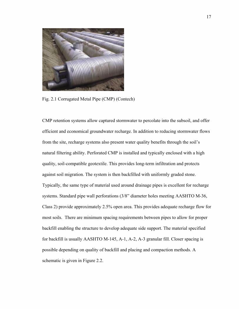
2.2 Corrugated Pipe
The most commonly used system to date is corrugated metal pipe (CMP) and Corrugated
Plastic Pipe (CPP). The pipe are connected in rows and tied into a manifold for inlet flow
as shown in Figure 2.1.
17
Fig. 2.1 Corrugated Metal Pipe (CMP) (Contech)
CMP retention systems allow captured stormwater to percolate into the subsoil, and offer
efficient and economical groundwater recharge. In addition to reducing stormwater flows
from the site, recharge systems also present water quality benefits through the soil’s
natural filtering ability. Perforated CMP is installed and typically enclosed with a high
quality, soil-compatible geotextile. This provides long-term infiltration and protects
against soil migration. The system is then backfilled with uniformly graded stone.
Typically, the same type of material used around drainage pipes is excellent for recharge
systems. Standard pipe wall perforations (3/8” diameter holes meeting AASHTO M-36,
Class 2) provide approximately 2.5% open area. This provides adequate recharge flow for
most soils. There are minimum spacing requirements between pipes to allow for proper
backfill enabling the structure to develop adequate side support. The material specified
for backfill is usually AASHTO M-145, A-1, A-2, A-3 granular fill. Closer spacing is
possible depending on quality of backfill and placing and compaction methods. A
schematic is given in Figure 2.2.

18
Pavement
Subbase
Crushed Stone
Pipe
Subgrade
Fig. 2.2 Schematic of Corrugated Pipe Storage System
The key to the design of these systems is an understanding of the interaction of the soil
envelope around a flexible pipe. Flexibility in buried pipes is a desired attribute and
understanding how the flexible pipe relates to its adjacent soils, thereby establishing a
functional pipe/soil composite structure, is the key to a successful design.
A buried pipe and its soil backfill will be subject to the earth embankment loads and live
loads in accordance with a fundamental principle of structural analysis: stiffer elements
will attract greater proportions of shared load than those that are more flexible. Given the
same well-compacted soils surrounding the pipe, the more flexible pipe attracts less
crown load than the rigid pipe of the same outer geometry. The surrounding soil is of
greater stiffness than the
flexible pipe and of lesser stiffness than the rigid pipe. For thermoplastic flexible
pipe, soil stiffer than the pipe settles less than the pipe displaces, thereby permitting
development of soil abutments, a necessary condition for the formation of a soil “arch.”

19
A second necessary condition is realized when the inter-granular shear strength of
properly compacted soil some distance above the pipe is mobilized to maintain its
geometry. The earth load on the crown of the pipe culvert is the portion between the
crown and some effective location of the soil arch. This load is less than the prism load –
a rectangular prism of earth extending from the top of the culvert surface to the top of the
embankment, with a base exactly the width of the outer dimensions of the culvert. For the
rigid structure, the more compliant soil adjacent to the pipe settles more than the pipe
decreases in height. The shear resistance provided by the soil contacts results in an earth
“pillar”, attracting a load greater than the prism load. To maximize the opportunity for
stress relaxation in a bedded pipe (and simultaneous transfer of load from pipe to soil),
and for creep to be negligible, the control of the selection, placement and compaction of
backfill is essential.
In a properly designed and constructed flexible pipe/soil composite, the stiffness of the
soil will be substantially greater than the stiffness of the pipe. The attributes of pipe
flexibility in a pipe/soil composite structure are manifested
in many ways. Proper installation will insure the following advantages:
• Denser soil at springline favors the development of more competent
‘abutments’ necessary for the development of a soil arch. Less dense soil
immediately above the crown also favors the development of a soil arch.
The presence of a competent soil arch reduces the proportion of gravity
loads attracted to the pipe.

20
• Denser soil at springline favors the development of lateral passive
pressure. Greater lateral passive pressure gives rise to moments, shears
and displacements opposing those that exist in the pipe in response to
gravity loads only.
• When a flexible pipe laterally elongates and vertically shortens in
response to gravity loads, it adds density and stiffness to the soil in the
vicinity of springline and reduces soil density and stiffness in the vicinity
of the crown. This results in a lesser proportion of prism load than would
otherwise be attracted to the crown. The vertical arching factor (VAF) is
the parameter that quantifies the proportion
of prism load interacting with the crown.
2.3 Corrugated Arch Chambers
One of the advantages of arch chambers is that they are flexible and can be configured
into beds or trenches of various shapes and sizes. These systems can be installed by hand
as shown in figure2.3.
Fig. 2.3 Installation of Corrugated Arch System (Stormtech)

21
These systems require clean angular stone below, between and above the chambers. The
storage capacity is calculated by using both the void space within the chambers and 40%
porosity within the stone. The chambers are installed with a minimum six inches spacing
between each unit and detailed as shown in Figure 2.4.
Pavement
Subbase
Crushed Stone
This spacing allows for soil arching of the angular stone between arches. The soil arch
developed around the chamber provides the structural integrity required to support the
pavement system above.
2.4 Concrete Vaults
Precast concrete vaults have been designed for high void space and high strength. They
also represent the highest cost storage systems available on the market today. Their
design is based on a structrual design that incorporates reinforcement within the concrete
to support the pavement structure above the system. Currently, there are several concrete
suppliers that supply various types of concrete arch chambers and box culverts for
Subgrade
Arch
Fig. 2.4 Corrugated Arch Installation Details (Stormtech)

22
stormwater storage as shown in Figure 2.5. They can be designed in heights from 3 to 18
feet and are placed on stone bedding or cast in place footings.
Fig. 2.5 Concrete Arches and Culverts (Terre Hill)
2.5 Plastic Stormwater Modules
Plastic modules are used as alternates to corrugated pipe and corrugated arch systems.
There are over a dozen different manufactures of plastic modules for stormwater storage.
Several examples are given in Figure 2.6. These systems are the most efficient in terms of
voids space. They vary from 90% to 95% void space, are easily assembled in the field,
light weight and some are made from recycled materials. The high void ratio reduces the
amount of excavation required on jobsite and reduces the footprint required to install. The
modular design allows the product to be shipped assembled or unassembled to jobsites to
be more cost effective. They are very lightweight and can be installed by hand so heavy
equipment is not required. The modular units can be stacked upon each other or installed
in various patterns making it easier to work around utilities and other obstructions.

23
(a) Raintank® (b) Brentwood Industries®
(c) Aquacell® (d) Cudo®
Fig. 2.6 Various Examples of Plastic Stormwater Modules
The use of these systems has raised many questions regarding the structural integrity of
the units because they are manufactured from plastic. The plastic modules are the sole
support the pavement above and in most cases do not rely on soils for additional support.
It should be noted that due to the physical properties of these materials, along with
several serious other concerns, will be the focus of this thesis.

24
Figure 2.7 represents a schematic of a typical cross section for a plastic module system.
In large storage areas the footprint of plastic modules can exceed 10,000 square feet in
area.
Pavement
Subbase
Plastic Modules
Subgrade
Fig. 2.7 Cross Section of Plastic Modules

25
CHAPTER 3. POLYMERS AND GEOSYNTHETICS
3.1 Background
Within the last hundred years there has been an evolution from naturally occurring
polymers to creation and use of synthetic polymers. The majority of the synthetic
polymers used today include, polyethylene, nylon, polypropylene and polyester. These
materials are created from low molecular weight materials such as oil.
The use of synthetic polymers ranges from food packaging to everyday building
materials. In most cases they are used as material substitutions for traditional materials.
Steel parts in cars have been replaced high strength plastics and glass bottles for
beverages have been replaced with polyester bottles.
Plastics continue to encompass many segments of many industries due to their light
weight, increased durability, increased design flexibility, low temperature impact
resistance, and efficient manufacturability.
The success of these materials and future applications depends largely on scientist’s and
engineer’s ability to understand the material properties and utilize the materials properly.
3.2 History
The first synthetic plastic was unveiled by Alexander Parkes at the 1862 Great
International Exhibition in London. This material; which the public dubbed Parkesine,
was an organic material derived from cellulose that once heated could be molded but that
retained its shape when cooled. Parkes claimed that this new material could do anything
rubber was capable of, but at a lower price. He had discovered something that could be
transparent as well as carved into thousands of different shapes. But Parkesine soon lost
its luster, when investors abandoned the product due to the high cost of the raw materials
needed in its production (Fenichell, 1996).

26
Bakelite was the next major breakthrough in resins. Working in a converted barn
laboratory on his estate overlooking the Hudson River, the independent chemist and
inventor Leo Baekeland created the first all-synthetic polymer in 1907. He was also
the first to call this new substance “plastic.” Baekeland’s process improved on
previous attempts at mixing phenol (from coal tar) and formaldehyde (from wood
alcohol) and markedly outperformed celluloid. Pressed into molds when heated,
Bakelite sturdily retained its shape upon cooling. Bakelite was used to make all
manner of goods, including knobs, brackets, insulation for electric cables, radios,
cups, buttons, cameras, telephones, false gums, and silverware handles (American
Chemistry Council). One of the drivers for its production was to replace the high
cost/low availability of ivory for billiard balls (Fenichell, 1996).
3.3 Definition and Properties
Macromolecules now called polymers are substances composed of monomers or
molecules that have long sequences of one or more atoms linked together by primary,
usually covalent bonds (Figure 1). Macromolecules are formed by linking together
monomer molecules through chemical reactions; this process is known as polymerization.
The polymerization of ethylene molecules with 50,000 carbon atoms linked together
creates polyethylene. See figure 3.1 where n = 50,000.

27
Fig. 3.1 – Polyethylene Polymer Chain (Plastics Engineering)
The definition implies that polymers have a linear structure and this is true for many
macromolecules. However, there are also polymers with non-linear structures such as
branched and network polymers. Branched structures have side chains of significant
length that are bonded to the main linear chain at junction or branch points. These
polymers are characterized by the number and size of branches. Network branches have
three-dimensional structures. Their linear chains have branches and are connected to
other linear chains by these branches. Network polymers are more commonly known as
crosslinked. They are described by their crosslinked density or degree of crosslinking.
Examples of both linear and crosslinked polyethylene are shown in Figure 3.2.
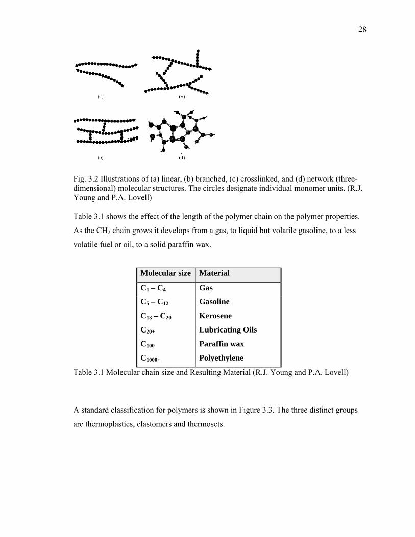
28
Fig. 3.2 Illustrations of (a) linear, (b) branched, (c) crosslinked, and (d) network (three-dimensional) molecular structures. The circles designate individual monomer units. (R.J. Young and P.A. Lovell)
Table 3.1 shows the effect of the length of the polymer chain on the polymer properties.
As the CH2 chain grows it develops from a gas, to liquid but volatile gasoline, to a less
volatile fuel or oil, to a solid paraffin wax.
Molecular size Material
C1 – C4 Gas
C5 – C12
C13 – C20
C20+
C100
C1000+
Gasoline
Kerosene
Lubricating Oils
Paraffin wax
Polyethylene
Table 3.1 Molecular chain size and Resulting Material (R.J. Young and P.A. Lovell)
A standard classification for polymers is shown in Figure 3.3. The three distinct groups
are thermoplastics, elastomers and thermosets.

29
Thermoplastics
Elastomers
Thermosets
Crystalline
Amorphous
Polymers
Fig. 3.3 – Polymer classification
Thermoplastics are the most commonly used polymers. They are referred to as plastic and
are the polymer focus for this research. They are linear or branched polymers that can be
melted by application of heat, molded and remolded into any shape through extrusion or
injection molding. This is due to the secondary van der Waals forces, dipoles and
hydrogen bonds that hold the polymer chains together. There are no crosslinked sites or
chains to fix the polymer chain in position. In general, a thermoplastic can be considered
a non-crosslinkable polymer.
Elastomers are crosslinked rubbery polymers that when stressed have high elongations of
up to 10 times their original size. They recover their original shape when the stress is
released. This property is a result of the molecular structure having a low crosslink
density. These polymers are commonly referred to as rubber and are used to describe
rubbery polymers that are not crosslinked.
Thermosets are rigid network polymers where the polymer chain is restricted from
movement by the high degree of crosslinking. Once a thermoset polymer is formed, the
crosslinks hold the shape of the material. Additional heat and pressure result in the
dislocation of crosslinks and cause degradation of the polymer.

30
Thermoplastics are further described as crystalline or amorphous. Crystalline implies the
polymer chain is an ordered pattern as opposed to a random pattern arrangement. A
random arrangement of the polymer chain implies amorphous and aligned polymer
chains implies crystalline. Figure 3.4 shows a description of both amorphous and
crystalline.
Fig. 3.4 Polymer chain alignments for both amorphous and crystalline material (G.R.
Moore and D.E. Kline)
This additional classification describes the molecular structure (order of the polymer
chains) and its associated properties. Theromplastics are processed with the use of heat.
Thermoplastics do not crystallize easily during cooling of the polymer to a solid state.
Polyethylene is (the most common thermoplastic polymer and the focus of this thesis)
generally divided into two main groups:
• Linear Low Density Polyethylene (LLDPE) at a density of 925-945 kg/m3
• High Density Polyethylene (HDPE) at a density of 940-960 kg/m3
HDPE was developed with a process that uses special catalysts at relatively low pressures
(below 4 MPa) and temperatures. LLDPE is made from a low pressure process by co-
polymerizing ethylene with a small amount of alpha-olefins (such as Butene-1, Pentene-
1, Hexene-1, and Octene-1) which lowers the density by forming short side chain
31
branches on the linear polymer chain. The key property differences between the two
polyethylenes show that HDPE is more rigid, stronger, and tougher and has better
chemical resistance. On the other hand, LLDPE is used where a less rigid material is
required, such as a geomembrane used in a landfill closure where differential settlement
and higher strains are expected.
Additives are used to increase end use properties such as durability, UV resistance,
thermal stability and antistatic properties. Polyethylene aged by long periods of exposure
to light, high temperature and moisture will deteriorate and become brittle. Two additives
used to greatly increase the useful life of polyethylene are antioxidants and carbon black
(about 2%). There are two types of antioxidents (AO’s) used during manufacturing. The
first are high temperature AO’s used for processing and the second are low temperature
and are used to increase the durability of the polymer. Antioxidants are used to slow the
oxidation process and carbon black is used to protect the polymer chain from UV
exposure by blocking its rays by its relatively large size.
Four main parameters control the processability and performance of polyethylene:
• Molecular weight (Melt Index)
• Molecular weight distribution
• Degree of crystalinity (Density)
• Amount and type of AO’s
Various HDPE’s are designed to meet both the processing and end-use requirements by
controlling the above parameters.
32
3.4 GEOSYNTHETICS Geosynthetics are the term used to describe a range of polymeric products used to solve
civil engineering problems. The term is generally regarded to encompass seven main
product categories: geotextiles, geogrids, geonets, geomembranes, geosynthetic clay
liners, geofoam and geocomposites. According to ASTM D4439, a geosynthetic is
defined as follows:
geosynthetic, n – a planar product manufactured from polymeric materials used
with soil, rock, earth or other geotechnical engineering related material as an
integral part of a human-made project, structure or system.
Currently they have many benefits over traditional construction materials such as ease of
installation, cost competitiveness and they are manufactured in a quality controlled
environment.
The polymeric nature of geosynthetics makes them suitable for use in the ground where
high levels of durability are required. Properly formulated, however, they can also be
used in exposed applications. Geosynthetics are available in a wide range of forms and
materials, each to suit a slightly different end use. These products have a wide range of
applications and are currently used in many civil, geotechnical, transportation,
geoenvironmental, hydraulic, and private development applications including roads,
airfields, railroads, embankments, retaining structures, reservoirs, canals, dams, erosion
control, stormwater control, sediment control, landfill liners, landfill covers, mining,
aquaculture and agriculture.

33
3.5 DESIGNING WITH GEOSYNTHETICS
“Designing with Geosynthetics” ( Koerner, 2005) describes in great detail various way of
calculating long term designs of geosynthetic materials primarily by using the “design-
by-function” approach.
When designing for long term performance of a geosynthetic, one must evaluate the type
of polymer selected and application of the geosynthetic. Once the ultimate strength of the
geosynthetic is determined, one must reduce that strength by partial reduction factors
such as: installation damage, chemical and biological damage and creep.
The basis of the design-by-function method also uses a global factor of safety. In the case
of a structural reinforcing geosynthetic, the factor of safety (FS) is formulated as follows:
FS = Tallow/Treqd
where FS = factor of safety
Tallow = allowable tensile strength from laboratory testing
Treqd = required tensile strength from the particular design being considered
Tallow must account for the site specific conditions including the potential for installation
damage, chemical or biological degradation and the effects of long term creep. As a
result, Tallow will be a significantly lower value than the ultimate tensile strength (Tult) of
the material which must be reduced before being used in a design.
The use of reduction factors is one way to achieve Tallow.

34
Tallow = Tult [1 / RFID x RFCR x RFCBD]
Where
Tult = ultimate tensile strength from a standardized tensile test
Tallow = allowable tensile strength to be used in a design equation
RFID = reduction factor for installation damage
RFCR = reduction factor for avoiding the effects of creep
RFCBD = reduction factor against chemical and biological degradation
The reduction factors listed above are a few of the standard ones used, although others
can be added based on site specific design. In cases where there is little or no effect in
one of these conditions, the reduction factor can be 1.0 or 1.1. In other cases, such as
creep, the reduction factors can be as high as 3.0 to 4.0. The Geosynthetic Institute (GSI)
has written a report (White Paper #4) entitled
“Reduction Factors (RFs) Used in Geosynthetic Design”. The report provides values for
reduction factors based on polymer types and applications.
To obtain the proper value for each design it is recommended to perform laboratory or
field testing to simulate the actual conditions expected in the field. Creep testing can be
performed by testing properties over 10,000 hours at various temperatures and
developing a set of curves and then by the use of Arrhenius modeling so as to obtain a
reduction factor. The Stepped Isothermal Method (ASTM D6992) is a “fast” test that can
be performed in a day (TRI Environmental).

35
3.6 Three Dimensional Geosynthetics
The definition of a geosynthetic states “a planar material…” and although there has been
a lot written on the design of each of the main categories listed previously, there has been
little written on the design of polymer based cubes for stormwater storage. There are only
a few geosynthetics that are considered in three dimensions and evaluated for the long
term structural performance. Geonets and geocomposites are standard products tested for
their long term compressive strength but Geofoam is the significant material. Examples
are shown in Figure 3.5. The transmissivity of a geonet is tested under a confining load
for 100 hours per GRI-GC8 test method. This test accounts for the reduction in flow due
to the compressive creep of the polyethylene ribs of the geonet. On the other hand,
geofoam which is used to construct highway embankments, is tested for long term
compressive strength and strains.
Fig. 3.5 Samples Geofoam (CETCO Contracting Services)

36
Due to their polymeric nature these products are controlled by viscoelastic behavior. This
viscoelastic behavior will appear as creep of the polymer. Physically, creep and stress
relaxation are strongly related because they are based on the same mechanistic
phenomenon. The rearrangement of the molecular chains during strains, partly in the
amorphous region(s) and partly in the crystalline regions where there is a “slip” between
the molecules.
Creep strain is the total strain at any given time that is produced by an applied load
during a creep test. The strain is increase based on the percentage of applied load. Figure
3.6 illustrates both the constant-stress creep-time curve and the set of associated
isochronous curves.

37
Fig. 3.6 Load Dependent Creep Curves (Geosynthetic Institute)
It is composed of an elastic portion and a nonelastic portion of strain. The non-elastic
strain is a combination of a recoverable portion (primary creep) and a permanent
deformation (secondary creep); see Figure 3.7.

38
Fig. 3.7 Creep Curve of Polyethylene (AAPS )
It is important to note that the creep of a thermoplastic is very dependent on the applied
load as compared to the ultimate load of the material being tested. Figure 3.8 shows the
creep curves for various polymers at 20% of ultimate load.

39
Fig. 3.8 Creep of Various Polymers at 20% Load (Koerner, 2005)
Fig. 3.9 shows the same polymers under a load that is 60% of ultimate. It shows the
dramatic effect the additional load has for both PE and PP.
Fig. 3.9 Creep of Various Polymers at 60% Load (Koerner, 2005)
These values have been used in the plastic pipe industry as shown by the set of design
curves listed in Figure 3.10 that show tensile creep response for high density
polyethylene pipe.

40
Fig. 3.10 Creep Response for Polyethylene Pipe (Nayyar, 2002)

41
CHAPTER 4. PAVEMENT DESIGN
4.1 Pavement Design and the Effects of Subgrade
Highways are divided into two categories; rigid and flexible. Rigid pavements have a
high modulus of elasticity and distribute loads over a relatively wide area of soil.
Variations in subgrade strength have little effect on the performance of rigid pavements.
Flexible pavements are built of relatively thin wearing course built over a base course and
subbase course and rest on a compacted subgrade. Flexible pavements have an asphalt
surface. Although a pavement's wearing course is most prominent, the success or failure
of a pavement is more often than not dependent upon the underlying subgrade, the
material upon which the pavement structure is built. Highways constructed over fine-
grained soils show higher levels of distress than those constructed over granular soils.
Subgrades can be composed of a wide range of materials although some are much better
than others. There is no known work that considers the use of three dimensional plastic
modules used as a subgrade. For the purpose of this thesis, the focus will be on asphalt
pavements.
Asphalt pavement design methods are based on controlling surface rutting and limit the
elastic strain at the top of the subgrade relying on two assumptions. Firstly, it is assumed
that most surface rutting is due to subgrade deformation rather than the combined
deformation of the overlying pavement layers. Secondly, it is assumed that the subgrade
plastic (permanent) deformation is related to the magnitude of its elastic (temporary or
recoverable) strain.

42
Plastics being viscoelastic materials are highly susceptible to deformation and creep. This
subsection discusses a few of the aspects of subgrade materials that make them either
desirable or undesirable and the typical tests used to characterize subgrades. The next
chapter reviews the effects of plastic modules when used as subgrade.
4.2 Subgrade Performance
A subgrade’s performance generally depends on three of its basic characteristics (all of
which are interrelated):
1. Load bearing capacity. The subgrade must be able to support loads transmitted
from the pavement structure. This load bearing capacity is affected by soil type
and degree of compaction and moisture content. A subgrade that can support a
high amount of loading without excessive deformation is required.
2. Moisture content. Moisture tends to affect a number of subgrade properties
including load bearing capacity, shrinkage and swelling. Moisture content can be
influenced by a number of things such as drainage, groundwater table elevation,
infiltration, or pavement porosity (which can be assisted by cracks in the
pavement). Generally, excessively wet subgrades will deform excessively under
load.
3. Shrinkage and/or swelling. Some soils shrink or swell depending upon their
moisture content. Additionally, soils with excessive fines content may be
susceptible to frost heave in northern climates. Shrinkage, swelling and frost
heave will tend to deform and crack any pavement type constructed over them.

43
Poor subgrade materials should be avoided if possible, but when it is necessary to build
over weak soils there are several methods available to improve subgrade performance:
• Removal and replacement (over-excavation). Poor subgrade soil can be removed
and replaced with high quality fill. Although this is simple in concept, it is
usually expensive. Table 4.1 shows typical over-excavation depths recommended
by the Colorado Asphalt Pavement Association (CAPA).
Table 4.1:Over-Excavation Recommendations (CAPA, 2000)
Subgrade Plasticity Index Depth of Over-Excavation Below
Normal Subgrade Elevation
10 – 20 0.7 meters (2 ft.)
20 – 30 1.0 meter (3 ft.)
30 – 40 1.3 meters (4 ft.)
40 – 50 1.7 meters (5 ft.)
More than 50 2.0 meters (6 ft.)
• Stabilization with a cementitious or asphaltic binder. The addition of an
appropriate binder such as lime, portland cement or emulsified asphalt can
increase subgrade stiffness and/or reduce swelling tendencies. Table 4.2
summarizes the Colorado Asphalt Pavement Association recommendations.

44
Table 4.2: Some Stabilization Recommendations (from CAPA, 2000)
Stabilization Material When Recommended
Lime
Subgrades where expansion potential
combined with a lack of stability is a
problem.
Portland Cement Subgrades which exhibit a plasticity
index of 10 or less.
Asphalt Emulsion
Subgrades are sandy and do not have an
excessive amount of material finer than
the 0.075 mm (#200) sieve.
• Marginally poor subgrade soils may be compensated for by using additional base
layers. These layers (usually of crushed stone – either stabilized or unstabilized)
serve to spread pavement loads over a larger subgrade area. This option is rather
perilous in that when designing pavements for poor subgrades the temptation may
be to just design a thicker section with more base material because the thicker
section will satisfy most design equations. However, these equations are in part
empirical and were usually not intended to be used in extreme cases. Thus, a thick
pavement structure over a poor subgrade will not necessarily make a good
pavement.
45
Clearly, subgrade characteristics and performance are influential in pavement structural
design. Characteristics such as load bearing capacity, moisture content and
expansiveness will influence not only structural design, but also long-term performance
and cost.
4.3 Stiffness/Strength Tests
Subgrade materials are typically characterized by their resistance to deformation under
load, which can be either a measure of their strength (the stress needed to break or
rupture a material) or stiffness (the relationship between stress and strain in the elastic
range or how well a material is able to return to its original shape and size after being
stressed). In general, the more resistant to deformation a subgrade is, the more load it can
support before reaching a critical deformation value. Three basic subgrade
stiffness/strength characterizations are commonly used in the U.S.: California Bearing
Ratio (CBR), Resistance Value (R-value) and elastic (resilient) modulus. Figure 4.1
gives comparisons for each.

46
Table 4.3 Guide for Estimating Subgrade Soil Strengths (Tensar Earth Technologies)
Although there are other factors involved when evaluating subgrade materials (such as
swell in the case of certain clays), stiffness is the most common characterization and thus
CBR, R-value and resilient modulus are discussed here.
4.3.1 California Bearing Ratio (CBR)
The California Bearing Ratio (CBR) test is a simple strength test that compares the
bearing capacity of a material with that of a well-graded crushed stone (thus, a high
quality crushed stone material has a CBR equal to 100%). It is primarily intended for,
but not limited to, evaluating the strength of cohesive materials having maximum particle
sizes less than 19 mm (0.75 in.) (AASHTO, 2000). The text was developed by the
California Division of Highways around 1930 and was subsequently adopted by
numerous states, counties, U.S. federal agencies and internationally. As a result, most
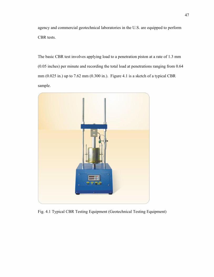
47
agency and commercial geotechnical laboratories in the U.S. are equipped to perform
CBR tests.
The basic CBR test involves applying load to a penetration piston at a rate of 1.3 mm
(0.05 inches) per minute and recording the total load at penetrations ranging from 0.64
mm (0.025 in.) up to 7.62 mm (0.300 in.). Figure 4.1 is a sketch of a typical CBR
sample.
Fig. 4.1 Typical CBR Testing Equipment (Geotechnical Testing Equipment)

48
4.3.2 CBR Sample
Values obtained are inserted into the following equation to obtain a CBR value:
⎟⎟⎠
⎞⎜⎜⎝
⎛=
yxCBR 100(%)
Eq. 4.1
Where: x = material resistance or the unit load on the piston (pressure)
for 2.54 mm (0.1in.) or 5.08 mm (0.2in.) of penetration
y = Standard unit load (pressure) for well graded crushed stone
= for 2.54 mm (0.1") penetration = 6.9 MPa (1000 psi)
= for 5.08 mm (0.2") penetration = 10.3 MPa (1500 psi)

49
The following table shows some typical CBR ranges.
Table 4.4 Typical CBR Ranges
General Soil Type USC Soil Type CBR Range
GW 40 – 80
GP 30 – 60
GM 20 – 60
GC 20 – 40
SW 20 – 40
SP 10 – 40
SM 10 – 40
Coarse-grained soils
SC 5 – 20
ML 15 or less
CL LL < 50% 15 or less
OL 5 or less
MH 10 or less
CH LL > 50% 15 or less
Fine-grained soils
OH 5 or less
Standard CBR test methods include AASHTO T 193: The California Bearing Ratio and
ASTM D 1883: Bearing Ratio of Laboratory Compacted Soils.
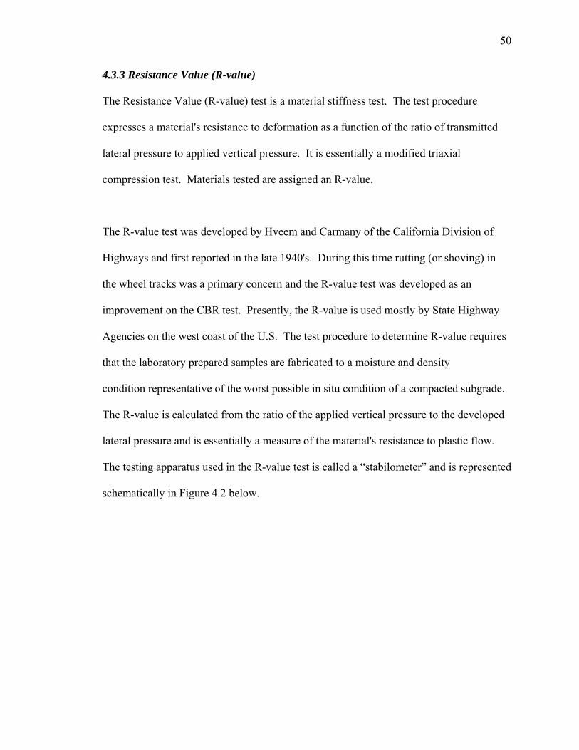
50
4.3.3 Resistance Value (R-value)
The Resistance Value (R-value) test is a material stiffness test. The test procedure
expresses a material's resistance to deformation as a function of the ratio of transmitted
lateral pressure to applied vertical pressure. It is essentially a modified triaxial
compression test. Materials tested are assigned an R-value.
The R-value test was developed by Hveem and Carmany of the California Division of
Highways and first reported in the late 1940's. During this time rutting (or shoving) in
the wheel tracks was a primary concern and the R-value test was developed as an
improvement on the CBR test. Presently, the R-value is used mostly by State Highway
Agencies on the west coast of the U.S. The test procedure to determine R-value requires
that the laboratory prepared samples are fabricated to a moisture and density
condition representative of the worst possible in situ condition of a compacted subgrade.
The R-value is calculated from the ratio of the applied vertical pressure to the developed
lateral pressure and is essentially a measure of the material's resistance to plastic flow.
The testing apparatus used in the R-value test is called a “stabilometer” and is represented
schematically in Figure 4.2 below.
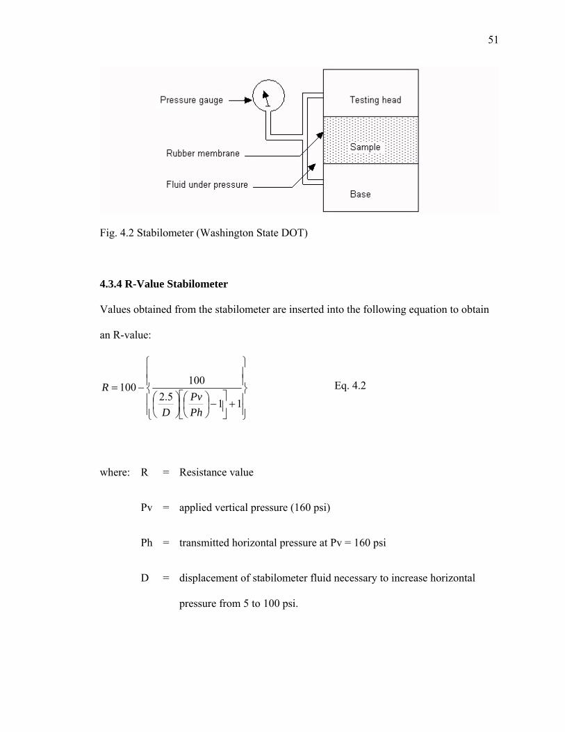
51
Fig. 4.2 Stabilometer (Washington State DOT)
4.3.4 R-Value Stabilometer
Values obtained from the stabilometer are inserted into the following equation to obtain
an R-value:
⎪⎪⎭
⎪⎪⎬
⎫
⎪⎪⎩
⎪⎪⎨
⎧
+⎥⎦
⎤⎢⎣
⎡−⎟
⎠⎞
⎜⎝⎛
⎟⎠⎞
⎜⎝⎛
−=115.2
100100
PhPv
D
R
Eq. 4.2
where: R = Resistance value
Pv = applied vertical pressure (160 psi)
Ph = transmitted horizontal pressure at Pv = 160 psi
D = displacement of stabilometer fluid necessary to increase horizontal
pressure from 5 to 100 psi.
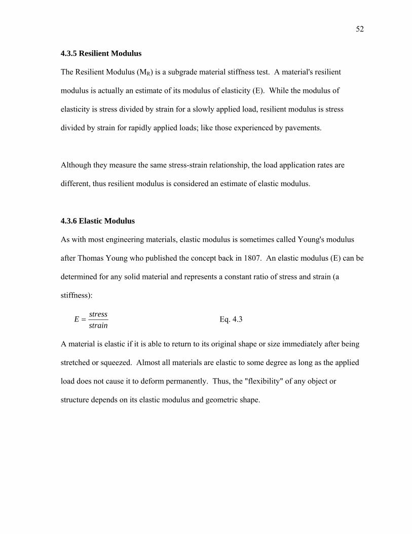
52
4.3.5 Resilient Modulus
The Resilient Modulus (MR) is a subgrade material stiffness test. A material's resilient
modulus is actually an estimate of its modulus of elasticity (E). While the modulus of
elasticity is stress divided by strain for a slowly applied load, resilient modulus is stress
divided by strain for rapidly applied loads; like those experienced by pavements.
Although they measure the same stress-strain relationship, the load application rates are
different, thus resilient modulus is considered an estimate of elastic modulus.
4.3.6 Elastic Modulus
As with most engineering materials, elastic modulus is sometimes called Young's modulus
after Thomas Young who published the concept back in 1807. An elastic modulus (E) can be
determined for any solid material and represents a constant ratio of stress and strain (a
stiffness):
strainstressE =
Eq. 4.3
A material is elastic if it is able to return to its original shape or size immediately after being
stretched or squeezed. Almost all materials are elastic to some degree as long as the applied
load does not cause it to deform permanently. Thus, the "flexibility" of any object or
structure depends on its elastic modulus and geometric shape.
53
4.3.7 Nomenclature and Symbols
The nomenclature and symbols from the 1993 AASHTO Guide is generally used in
referring to pavement moduli. For example:
EAC = asphalt elastic modulus
EBS = base course resilient modulus
ESB = subbase course resilient modulus
MR (or ESG) = roadbed soil (subgrade) resilient modulus (used interchangeably)
4.3.8 Triaxial Resilient Modulus Test
There are two fundamental approaches to estimating elastic moduli – laboratory tests and
field deflection data/back calculation. This section discusses laboratory tests. Of the
laboratory tests, two are noted:
• Diametral resilient modulus.
• Triaxial resilient modulus. This test is typically used on unbound materials such
as soil and aggregate and is covered here.
In a triaxial resilient modulus test a repeated axial cyclic stress of fixed magnitude, load
duration and cyclic duration is applied to a cylindrical test specimen. While the specimen
is subjected to this dynamic cyclic stress, it is also subjected to a static confining stress
provided by a triaxial pressure chamber. The total resilient (recoverable) axial
deformation response of the specimen is measured and used to calculate the resilient
modulus using the following equation:
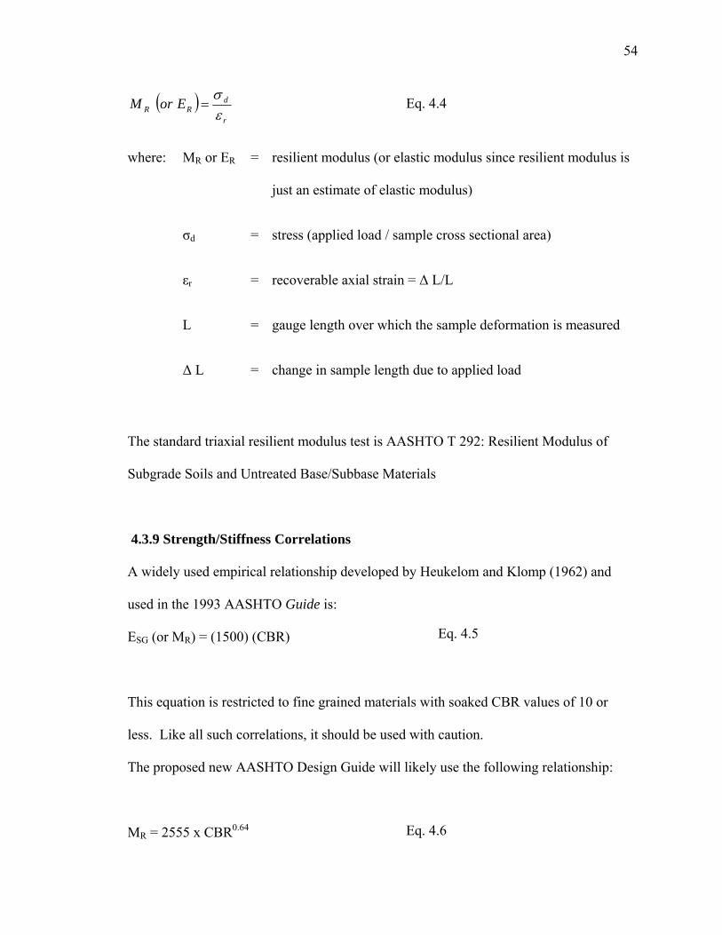
54
( )r
dRR EorM
εσ
=
Eq. 4.4
where: MR or ER = resilient modulus (or elastic modulus since resilient modulus is
just an estimate of elastic modulus)
σd = stress (applied load / sample cross sectional area)
εr = recoverable axial strain = Δ L/L
L = gauge length over which the sample deformation is measured
Δ L = change in sample length due to applied load
The standard triaxial resilient modulus test is AASHTO T 292: Resilient Modulus of
Subgrade Soils and Untreated Base/Subbase Materials
4.3.9 Strength/Stiffness Correlations
A widely used empirical relationship developed by Heukelom and Klomp (1962) and
used in the 1993 AASHTO Guide is:
Eq. 4.5 ESG (or MR) = (1500) (CBR)
This equation is restricted to fine grained materials with soaked CBR values of 10 or
less. Like all such correlations, it should be used with caution.
The proposed new AASHTO Design Guide will likely use the following relationship:
Eq. 4.6 MR = 2555 x CBR0.64

55
The 1993 AASHTO Guide offers the following correlation equation between R-value
and elastic modulus for fine-grained soils with R-values less than or equal to 20.
ESG (or MR) = 1,000 + (555)(R-value)
Eq. 4.7
4.3.10 Modulus of Subgrade Reaction (k)
The modulus of subgrade reaction (k) is used as a primary input for rigid pavement
design. It estimates the support of the layers below a rigid pavement surface course (the
PCC slab). The k-value can be determined by field tests or by correlation with other
tests. There is no direct laboratory procedure for determining k-value.
The modulus of subgrade reaction came about because work done by Westergaard during
the 1920s developed the k-value as a spring constant to model the support beneath the
slab as shown in figure 4.3.
Fig. 4.3 Spring Constant Illustrated
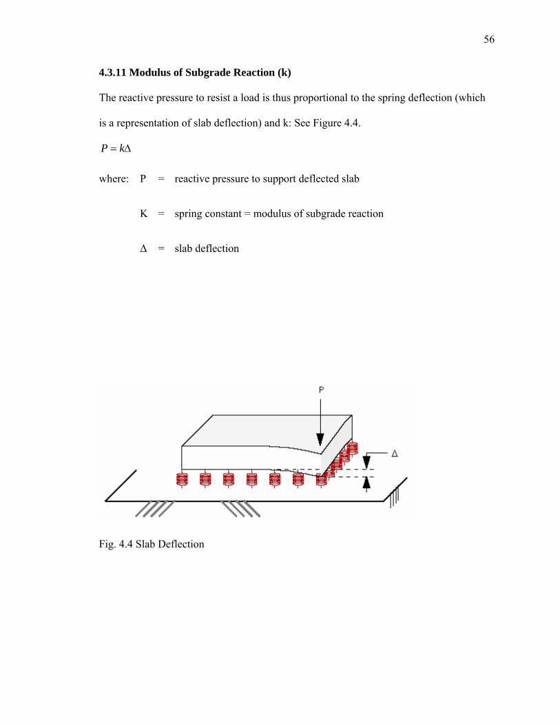
56
4.3.11 Modulus of Subgrade Reaction (k)
The reactive pressure to resist a load is thus proportional to the spring deflection (which
is a representation of slab deflection) and k: See Figure 4.4.
Δ= kP
where: P = reactive pressure to support deflected slab
K = spring constant = modulus of subgrade reaction
Δ = slab deflection
Fig. 4.4 Slab Deflection

57
4.3.12 Relation of Load, Deflection and Modulus of Subgrade Reaction (k)
The value of k is in terms of MPa/m (pounds per square inch per inch of deflection, or
pounds per cubic inch - pci) and ranges from about 13.5 MPa/m (50 pci) for weak
support, to over 270 MPa/m (1000 pci) for strong support. Typically, the modulus of
subgrade reaction is estimated from other strength/stiffness tests, however, in situ values
can be measured using the plate bearing test.
4.3.13 Plate Load Test
The plate load test presses a steel bearing plate into the surface to be measured with a
hydraulic jack (see figure 4.5). The resulting surface deflection is read from dial
micrometers near the plate edge and the modulus of subgrade reaction is determined by
the following equation:
Eq. 4.8
where: K = spring constant = modulus of subgrade reaction
P = applied pressure (load divided by the area of the 762 mm (30 inch)
diameter plate)
Δ = measured deflection of the 762 mm (30 inch) diameter plate
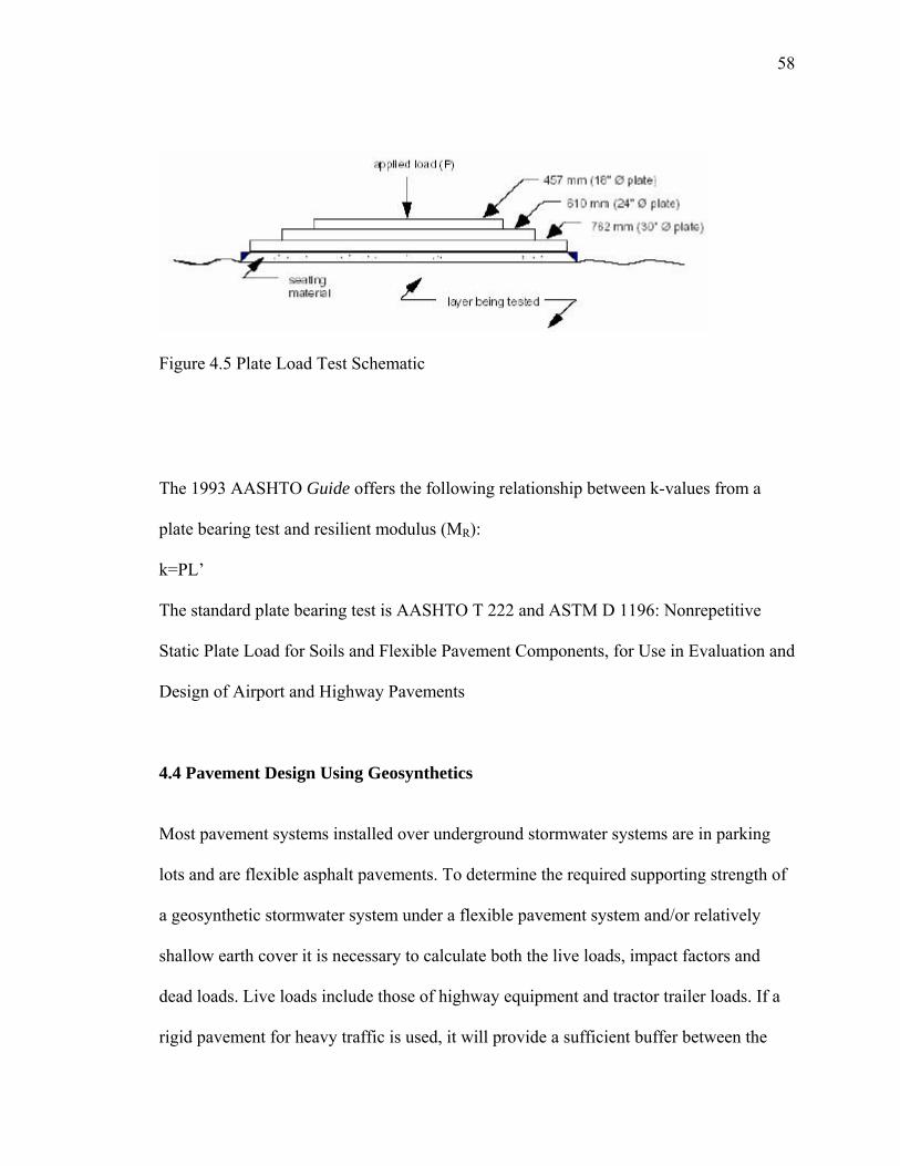
58
Figure 4.5 Plate Load Test Schematic
The 1993 AASHTO Guide offers the following relationship between k-values from a
plate bearing test and resilient modulus (MR):
k=PL’
The standard plate bearing test is AASHTO T 222 and ASTM D 1196: Nonrepetitive
Static Plate Load for Soils and Flexible Pavement Components, for Use in Evaluation and
Design of Airport and Highway Pavements
4.4 Pavement Design Using Geosynthetics
Most pavement systems installed over underground stormwater systems are in parking
lots and are flexible asphalt pavements. To determine the required supporting strength of
a geosynthetic stormwater system under a flexible pavement system and/or relatively
shallow earth cover it is necessary to calculate both the live loads, impact factors and
dead loads. Live loads include those of highway equipment and tractor trailer loads. If a
rigid pavement for heavy traffic is used, it will provide a sufficient buffer between the

59
live load of the buried geosynthetic and the live load transmitted is negligible. Dead loads
are both soil loads and surcharge loads. The weight of soil above the geosynthetic will
transfer a load to the geosynthetic based on the unit weight of the soil. The AASHTO
design loads commonly used are HS20 with a 32,000 pound axle load in the Normal
Truck Configuration and a 24,000 pound axle load in the Alternate Load Configuration.
The average wheel load is calculated as follows:
w = P(1 + IM)/A
where: w = wheel load average pressure intensity (psf)
P = total live wheel load applied at the surface (lbs)
A = spread wheel load area on top of the geosynthetic (sq.ft.)
IM = dynamic load allowance
The AASHTO LRFD Standard applies a dynamic load allowance to account for the truck
load being non-static. The dynamic load allowance IM, is determined by
IM = 33(1.0-0.125H)/100
Where H = height of soil cover above the top of the geosynthetic
The AASHTO LRFD design loads are the HS20 with a 32,000 pound axle load in the
Normal Truck Configuration and a 25,000 pound axle load in the Alternate Load
Configuration. The HS 20, 32,000 pound and the Alternate Truck 25,000 pound design
axle load are carried on dual wheels as shown on Figure 4.6. The contact area of the dual
wheels with the ground is assumed to be rectangular with the dimensions of 20 inches x
10 inches.
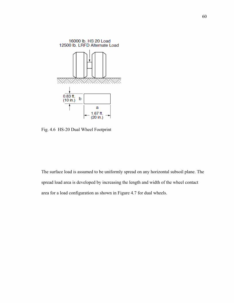
60
Fig. 4.6 HS-20 Dual Wheel Footprint
The surface load is assumed to be uniformly spread on any horizontal subsoil plane. The
spread load area is developed by increasing the length and width of the wheel contact
area for a load configuration as shown in Figure 4.7 for dual wheels.

61
Fig. 4.7 Wheel Contact Area and Load Spread Area
On the horizontal plane, the dimensions of the spread area increases the wheel contact
area based on the height of the soil cover over the geosynthetic and can vary for different
types of soils. When select granular materials are used for the soil cover, the spread area
can be increased by a factor of 1.15. For all other soils, a factor of 1.0 is used and results
in no spread of the foot print area. The spread area realized on top of the geosynthetic is
as follows:
Wheel Contact area = a x b
Spread a = a + 1.15H and Spread b = b+1.15H
Therefore spread A = (a + 1.15H) x (b + 1.15H)
In many cases, a geogrid is recommended to further increase the spread area. There has
been a lot of research by various geogrid and geotextile manufacturers as well as many
consultants over two decades. The effects of geogrids spreading loads and design values
are available from design guides such as “Spectra Pave” from the Tensar Corporation.
When a geogrid is used in conjunction with select granular material it has been shown
that as granular soil interlocks within the geogrid apertures it ties the soil together and

62
increases the load spreading of the granular soils. Geogrids are usually placed at the
bottom of a base layer but can also be incorporated within the base layer to promote
interlock of the granular material within the apertures of the geogrid. Figure 4.8 shows
the load distribution of the wheel load on the subbase and subgrade.
Subbase
Pavement
Subgrade
Fig. 4.8 Distribution of Wheel Load on Subbase and Subgrade
For the purpose of this research, the area of concern is the applied load at the top of the
subbase layer. Once calculated, the load applied can be used to calculate the deflection on
the plastic stormwater retention modules.
Figure 4.9 is a graph of the effects of an HS20 loading combined with the dead load over
a varied depth of soil covers up to 7.5 feet deep. It is based on a 16,000 lb wheel load and
a unit weight of 130 pcf for the cover soil. It shows the effects of the live load are

63
dramatic when the cover soils are less than 3 feet in height and that the dead load of the
cover soil is very small. It also shows that the effects of dead loads to not contribute
significantly until after 7 feet cover soil are placed. From this curve the combined live
and dead loads for 3 feet to 7 feet of cover can be 1,300 lb/ft2.
-
2,000
4,000
6,000
8,000
10,000
12,000
14,000
16,000
18,000
SoilCover
0 6 12 18 24 30 36 42 48 54 60 66 72 78 84
inches
PSF
w(psf) DL w+DL
Fig. 4.9 Dead Load and Live Load at Various Depths
4.5 Commentary
Subgrade properties are essential pavement design parameters. Materials typically
encountered in subgrades are characterized by their strength and their resistance to

64
deformation under load (stiffness). In the U.S., the CBR, R-value and resilient modulus
are commonly used to characterize subgrade materials.
Although each method is useful, the resilient modulus is most consistent with other
disciplines and is gaining widespread use in pavement design. The modulus of subgrade
reaction (k) is the subgrade characterization used in rigid pavement design. It can be
estimated from CBR, R-value or elastic modulus, or calculated from field tests like the
plate bearing test.
The introduction of plastic stormwater retention modules requires additional testing to
evaluate their performance and predict the stiffness and/or amount of deflection for
proper pavement design. Although the elastic modulus of a plastic module can be
measured, there is no current method to relate it to the Resilient Modulus.

65
CHAPTER 5. TESTING PROGRAM
Currently, there are no standards for testing plastic stormwater retention modules. This
chapter reviews the stress strain relationship for plastics and testing is performed to
evaluate the plastic modules. A testing program was developed to determine both the
yield strength and ultimate strength of the fully assembled Plastic Stormwater Retention
Module (PSRM) as well as the amount of deformation in each unit. Deformation that
occurs upon loading can be classified as either elastic or plastic. Elastic deformation is
recovered immediately upon unloading. Plastic deformation is not recovered after
unloading and is therefore permanent. Once plastic deformation begins, only a small
increase in stress usually causes a relatively large additional deformation. Materials with
large amounts of plastic deformation behave in a ductile manner and include low strength
metals and in this case polyethylene.
5.1 Strength of Materials
One way to characterize the behavior of any material is to calculate its modulus. The
modulus of elasticity for a material is the slope of its stress-strain plot within the elastic
range, as shown in Figure 5.1.

66
Fig. 5.1 Stress strain curve
Fig. 5.2 Modulus Calculation from a Stress Strain Curve of Steel

67
The initial straightline portion of the curve is the elastic range for the steel. If the
material is loaded to any value of stress in this part of the curve, it will return to its
original shape upon the release of load. Thus, the modulus of elasticity is the slope of
this part of the curve and is equal to about 207,000 MPa (30,000,000 psi) for steel. It is
important to remember that a measure of a material's modulus of elasticity is not a
measure of strength. Strength is the stress needed to break or rupture a material, whereas
elasticity is a measure of how well a material returns to its original shape and size.
Table 5.1 Typical Modulus of Elasticity Values for Various Materials (Washington State DOT)
Elastic Modulus Material
MPa Psi
Diamond 1,200,000 170,000,000
Steel 200,000 30,000,000
Aluminum 70,000 10,000,000
Wood 7,000-14,000 1,000,000-2,000,000
HDPE 2,500 170,000
Crushed Stone 150-300 20,000-40,000
Silty Soils 35-150 5,000-20,000
Clay Soils 35-100 5,000-15,000
Rubber 7 1,000

68
Stress versus stain curves vary by material. There is a great deal of variability even within
plastics themselves. Figure 5.3 shows a range of stress strain curves for various plastics.
Fig 5.3 Stress Strain curves for various plastics (Azom Materials)
5.2 Plastic Stormwater Retention Module Testing
Although there are several manufacturers of plastic cube stormwater systems two
manufacturers were selected to be tested. They will be referred to as Product “A” and
Product “B”. These systems were selected because both are similar in structure and have
the same dimensions. Each can be constructed with 2 to 5 inserts for increased structural
support. See Figure 5.4 for an expanded example.
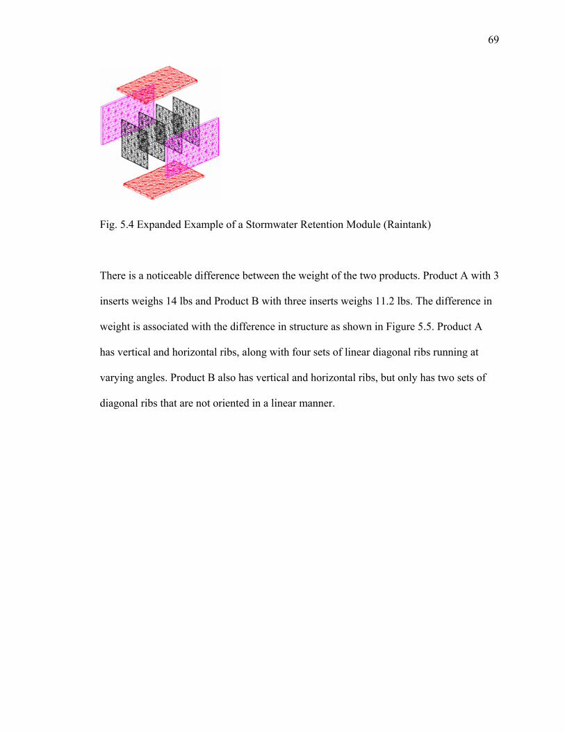
69
Fig. 5.4 Expanded Example of a Stormwater Retention Module (Raintank)
There is a noticeable difference between the weight of the two products. Product A with 3
inserts weighs 14 lbs and Product B with three inserts weighs 11.2 lbs. The difference in
weight is associated with the difference in structure as shown in Figure 5.5. Product A
has vertical and horizontal ribs, along with four sets of linear diagonal ribs running at
varying angles. Product B also has vertical and horizontal ribs, but only has two sets of
diagonal ribs that are not oriented in a linear manner.
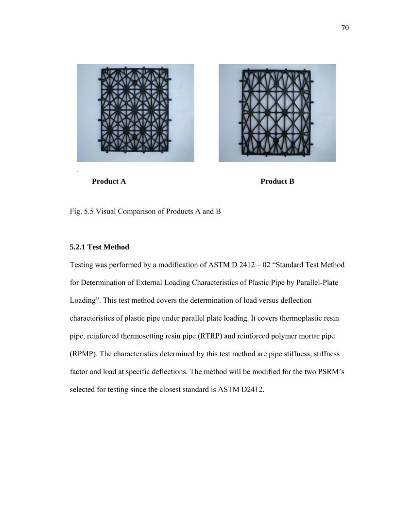
70
.
Product A Product B
Fig. 5.5 Visual Comparison of Products A and B
5.2.1 Test Method
Testing was performed by a modification of ASTM D 2412 – 02 “Standard Test Method
for Determination of External Loading Characteristics of Plastic Pipe by Parallel-Plate
Loading”. This test method covers the determination of load versus deflection
characteristics of plastic pipe under parallel plate loading. It covers thermoplastic resin
pipe, reinforced thermosetting resin pipe (RTRP) and reinforced polymer mortar pipe
(RPMP). The characteristics determined by this test method are pipe stiffness, stiffness
factor and load at specific deflections. The method will be modified for the two PSRM’s
selected for testing since the closest standard is ASTM D2412.

71
5.2.2 Procedure
1. Determine the dimensions of each unit to the nearest 1 mm by making and
averaging at least 4 equally spaced measurements in each direction
2. Measure the thickness of each rib section of the unit. Make eight measurements
equally spaced to calculate the average thickness.
3. Attach an identification tag with manufactures code, unit test number, ambient
temperature and test number.
4. Locate the centerline of the unit and center the unit within both bearing plates
5. Insert a deflection indicator and bring upper plate into contact just enough to hold
unit in place. This will establish the starting point for deflection measurements.
6. Compress the unit at a constant rate of 0.50+/- 0.02 in./min. (12.5+/- 0.5mm)/min.
7. Record load deflection measurements continuously.
8. Observe and note the load and deflection at the first evidence of each of the
following significant events when and if they occur:
a. Cracking or crazing
b. Rupture or collapse
9. Record type and position of each event with the corresponding load and
deflection. Stop test when either of the following occur:
a. The load fails to increase with increased deflection
b. The unit deflection reaches 30% of the average height of the unit or total
failure of the unit

72
5.2.3 Calculations
1. Calculate the unit stiffness, US, for any given deflection as follows:
US = F/Δy lb/(in./in.) (kPa) Eq. 5.1
The in./in. units is based on the deflection/height of unit
Where F = load applied
Δy = deflection
2. Calculate the unit deflection percentage P as follows:
P = Δy/h x 100 Eq. 5.2
Where h= height of PSRM
5.2.4 Report
1. Report the following information:
a. Complete identification of the material tested, include type of unit,
source, manufacture’s code, and unit identification.
b. Dimensions of each unit including rib thickness and number of internal
support plates if any.
c. Conditioning and testing temperature, time and environment.
d. The load and deflection at which the following occurs:

73
i. Unit cracking or crazing
ii. Load and deflection at rupture
iii. Reason for terminating test.
iv. Plot the load versus deflection and note the following:
1. Unit cracking or crazing
2. Rupture
v. Unit stiffness, F/ Δy, at 5 and 10% deflection for each unit
vi. If cracking or rupture occurs below 5% deflection calculate unit
stiffness at the percentage deflection where either event occurs
e. Date of test
5.2.5 Phase 1(a) Testing
Single unit test
Product A and Product B supplied by ACF Environmental
Test units from each manufacturer and vary the number of inserts.

74
First test completed using a rigid load plate.
Fig. 5.6 Testing of Product A with Three Internal Plates between Rigid End Plates
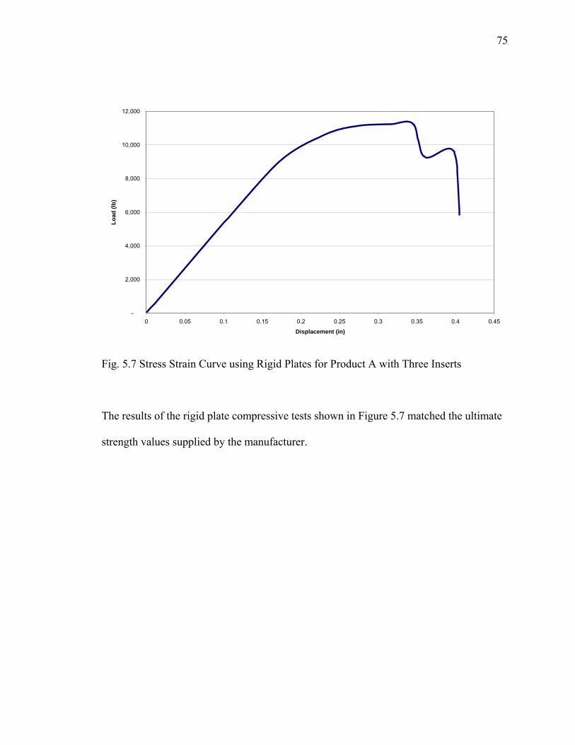
75
Rigid Plates - Product A3 Inserts
-
2,000
4,000
6,000
8,000
10,000
12,000
0 0.05 0.1 0.15 0.2 0.25 0.3 0.35 0.4 0.45
Displacement (in)
Load
(lb)
Fig. 5.7 Stress Strain Curve using Rigid Plates for Product A with Three Inserts
The results of the rigid plate compressive tests shown in Figure 5.7 matched the ultimate
strength values supplied by the manufacturer.

76
5.2.6 Phase 1(b) Testing
Single unit tested unconfined with tapered flexible load plate
Test with 3, 4 and 5 inserts
Fig. 5.8 Testing of Product A Three Inserts using a Flexible End Plate

77
Flexible - Product A3 Inserts
-
1,000
2,000
3,000
4,000
5,000
6,000
7,000
0 0.1 0.2 0.3 0.4 0.5 0.6 0.7
Displacement (in)
Load
(lb)
Fig. 5.9 Stress Strain Curve of Product A with Three Inserts using a Flexible End Plate
Test results using the flexible plate and 3 inserts resulted in almost half of the ultimate
strength and less than half the yield strength as shown in Figure 5.9.
5.2.7 Phase 2(a) Testing
Two different methods were used to create confinement for Product A. For the rigid
confined test, the units are confined be two outer panels connected by four equally spaced
threaded steel rods as shown in Figure 5.10 and resulting stress versus strain curve in
Figure 5.11.
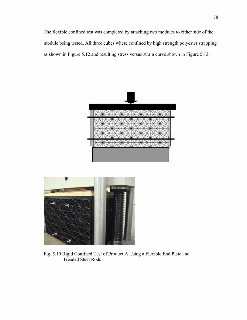
78
The flexible confined test was completed by attaching two modules to either side of the
module being tested. All three cubes where confined by high strength polyester strapping
as shown in Figure 5.12 and resulting stress versus strain curve shown in Figure 5.13.
Fig. 5.10 Rigid Confined Test of Product A Using a Flexible End Plate and Treaded Steel Rods
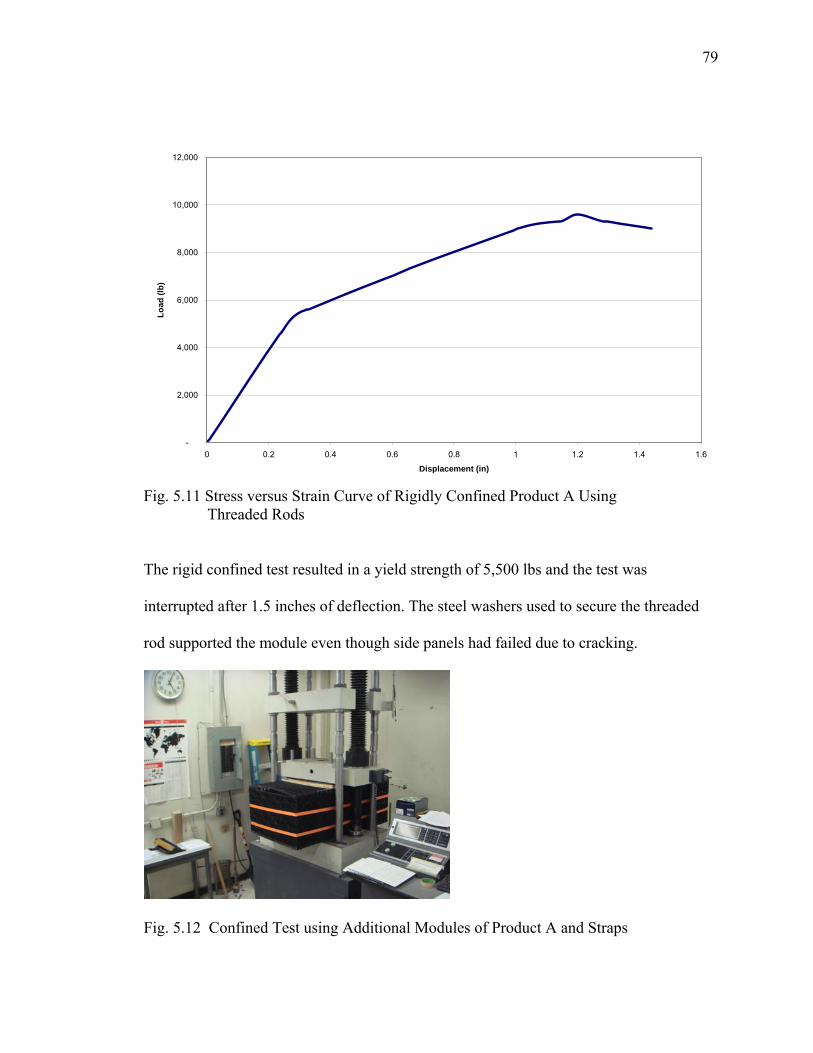
79
Flexible & Confined by Threaded Bar3 Inserts
-
2,000
4,000
6,000
8,000
10,000
12,000
0 0.2 0.4 0.6 0.8 1 1.2 1.4 1.6
Displacement (in)
Load
(lb)
Fig. 5.11 Stress versus Strain Curve of Rigidly Confined Product A Using
Threaded Rods
The rigid confined test resulted in a yield strength of 5,500 lbs and the test was
interrupted after 1.5 inches of deflection. The steel washers used to secure the threaded
rod supported the module even though side panels had failed due to cracking.
Fig. 5.12 Confined Test using Additional Modules of Product A and Straps

80
Flexible & Confined by Straps3 Inserts
-
1,000
2,000
3,000
4,000
5,000
6,000
7,000
8,000
9,000
0 0.2 0.4 0.6 0.8 1 1
Displacement (in)
Load
(lb)
.2
Fig. 5.13 Stress versus Strain Curve of Flexible Confined Test by Using Polyester Straps
The confined test resulted in a yield strength of 4,700 lbs but gave a more realistic failure
within the module where the load was applied.
5.2.8 Phase 4 testing cycled loading
Unconfined module loaded, load held, reduced to 50% load, increased to 75% load, load
released and increased to 50% load as shown in Figure 5.14. The maximum load was
reached through each cycle but displacement occurred within the sample.

81
Flexible - Cycled Loading
-
1,000
2,000
3,000
4,000
5,000
6,000
7,000
0 0.1 0.2 0.3 0.4 0.5 0.6
Displacement (in)
Load
(lb)
Fig. 5.14 – Stress versus Strain of Cyclic Loading for Product A
5.3 TEST RESULTS
Product A was reasonable well behaved during the various testing configurations.
However, during the testing of Product B the values varied greatly and were very
inconsistent with those of Product A. Further investigation of Product B showed that the
PSRM was produced from two different polymer sources. The outer panels all failed in a
ductile manner while the internal inserts failed in a brittle manner. Upon observation of
the broken inner panels a honeycomb of air bubbles were noticed. These samples were
viewed under a microscope and it became obvious that the bubbles where a result of
impurities in the polymer that most likely created gases during the extrusion process and

82
thus the bubbles. These impurities are usually a result of poor selection or incomplete
processing of recycled materials and lack of attention to the amount of cleaning of the
recycled plastic prior to processing. This would also support the issues with the varying
test results of the same system. As a result of these findings, all further testing was
conducted using Product A. Each of the tests results were plotted together in Figure 5.15
and given in Table 5.2.
-
2,000
4,000
6,000
8,000
10,000
12,000
0 0.2 0.4 0.6 0.8 1 1.2 1.4 1.6
Displacement (in)
Load
(lb)
Rigid Plate Flexible Plate Confined Bar Confined Straps Cycled
Fig. 5.15 Comparison of Stress Strain Curves for Each Test

83
Table 5.2 Results of Compression Tests Configuration Load at yield
(lbs) Maximum Load (lbs)
US lbf/(in/in)
P
Product A (3) Rigid Plate 9,300 11,200 900,000 1.02Product A (3) inserts 4,800 6,400 348,000 1.36Product A (3) confined flexible
4,900 9,500 362,000 1.36
Product A (3) confined rigid 6,000 8,100 471,100 1.88Product A (4) inserts 5,500 7,900 405,800 1.36Product A (5) inserts 7,100 8,200 515,500 1.36 During testing it became obvious that the rigid plates used for compression obtained the
highest yield and ultimate strengths as shown in Figure 5.16. The structure of the box was
tested and did not deform until failure. At failure it was observed that the pins used to
connect each panel together flexed until snapping off or breaking.
The cubes loaded with a flexible plate deformed on the longitudinal side of the box until
failure. Failure was observed when the exterior plate flexed enough to “pop” out of the
cube.

84
-
2,000
4,000
6,000
8,000
10,000
12,000
3 rigid plates 3 inserts 4 inserts 5 inserts 3 confined flexible 3 confined rigid
lbs
0
0.05
0.1
0.15
0.2
0.25
0.3
0.35
in
Load at Yield Load at Failure Strain Δy at yield
Fig. 5.16 Comparison of Tests Results for Product A
In both cased the interior panels were observed to flex in either direction during the
loading of the upper surface; see Figure 5.17.
Fig. 5.17 (a) External View of Failed Module and (b) Internal View of Failed Module

85
It can be seen in each case that the mode of failure is the buckling of both internal and
external panels. This bending is best explained by Euler’s formula.
Leonhard Euler first derived a series of equations to determine the deformation of
columns under loads as shown in Figure 5.18. The formula derived is given in equation
5.3
Pcr = π2EI/Le2 Eq. 5.3
Where
Pcr = Critical Load
E = the elastic modulus
I = moment of inertia
Le = the effective length
Fig. 5.18 First Three Column Buckling Modes (University of Oklahoma)

86
The method of support determines the effective length and there are four options:
(a) one fixed end, one free end, where Le = 2L
(b) both ends pinned, where Le = L
(c) one fixed end, one pinned end, where Le = 0.7L
(d) both ends fixed, where Le = 0.5L
The length is a square value and drives the formula. For the purpose of this thesis, we are
evaluating columns of the same length and moment of inertia, so the elastic modulus of
the material used will have the largest effect on the critical load.
87
CHAPTER 6. CURRENT PROBLEMS WITH PLASTIC STORMWATER
RETENTION MODULE SYSTEMS
Plastic stormwater systems have only been in use for several years. To date most projects
have been installed successfully with some exceptions. As these products gain more
acceptance in the market their use will increase and the applications and design of these
systems will be challenged.
6.1 Failures
To date there have been several failures of plastic modules. Most have occurred during
installation and a few have occurred while in service.
One of the earlier failures was of a corrugated arch chamber. To create more storage, an
insert was placed to span between arches. Although this created more void space it
eliminated any soil arching potential and greatly reduced the structural integrity of the
system; see Figure 6.1.

88
Fig. 6.1 Soil Arch Eliminated from Arching Over Main Chambers (Zallen Engineering)
Unfortunately, the system had been installed and paved over prior to its catastrophic
failure; see Figure 6.2.
Fig. 6.2 Failed Stormwater System under Asphalt Pavement (Zallen Engineering)

89
One of the larger failures occurred at a landfill site on Long Island (see figure 6.3) while
in service, but before a concrete pavement was installed. The system installed was a
recycled plastic cube module required to store over 500,000 cubic feet of stormwater.
The design included seven modules stacked vertically (10 ft.) with four to six feet of
cover soil and a concrete wearing surface. After installation of the modules and cover
soils, fully loaded articulating dump trucks drove above the system.
Fig. 6.3 Failed Stormwater System at Landfill, Long Island, NY
These failures and others are a result of many different, site specific and product specific
factors.

90
6.2 Resin Selection
Unlike the rest of the geosynthetic industry which use virgin resins, many manufacturers
of PSRM’s use many different grades of polymer resin and in some cases use recycled
resins. Some of the samples tested varied in color, weight and density. These variations
within the same product are a sign of variable raw materials. A review of each
manufacturer’s specification reveals nothing regarding the source or quality of the
polymer resin. In one case, samples examined after failure showed honeycombing within
the polymer, see Figure 6.4.
Fig. 6.4 Failed Sample of Recycled Product
This can be a sign of poor injection molding or more likely the result of contaminated
recycled material. The “dirty” recycled material will give off gasses as the polymer is
melted and remains trapped in the form of voids or impurities.

91
6.3 Manufacturing Quality Control (MQC) and Assurance (MQA)
Proper MQC/MQA provides a paper trail from resin selection to production of the final
product. Paperwork must include the source of resin any additives and the various index
test results. Test results should include density, melt index and other polymer index tests.
There should also be a set of MQC results for physical properties tested of the final
product. Each production run or lot should be tied back to the raw material used in its
production. Currently, the only thing supplied from most PSRM manufacturers is a one
page specification with little to no MQC/MQA data. Testing of the finished product is
left to the design engineer or third party inspection engineer. It is also their responsibility
to develop the testing program as there is no direction given by most manufacturers, see
Appendix A for a proposed specification in this regard.
6.4 Testing Criteria
There are no current test methods for plastic stormwater modules. Each manufacturer has
developed their own test or set of tests. Additionally, each manufacturer reports the
ultimate strength and does not provide the stress versus strain curve for a design engineer
to review. This results in the design engineer to rely solely on over estimated strengths.
The test method used for thesis was based on ASTM D4212, Standard Test Method for
Determination of External Loading Characteristics of Plastic Pipe by Parallel Loading.
This method was chosen as the closest ASTM Method available for testing plastic
stormwater modules. It was modified to allow for the use of a flexible plate instead of the
rigid plate specified in the test method. The stress strain curves from testing were used to

92
determine the yield strength and calculations can be performed using strengths within the
elastic region of the polymer.
6.5 Factor of Safety Design
A few of the manufacturers list a single Factor of Safety (FS) based on compressive test
results of each module. These results do not consider the depth of cover soil or creep
reduced strength. As shown in Figure 6.5 the effects of a live load are extremely high
within the first 24 inches of cover. After 36 inches of cover the composite load levels out
until the cover soil exceeds 48 inches. After 48 inches the dead load slowly starts to have
an effect on the total load.
Dead Load vs Live Load (w)
-
2,000
4,000
6,000
8,000
10,000
12,000
14,000
16,000
18,000
SoilCover
0 6 12 18 24 30 36 42 48 54 60 66 72 78 84
inches
PSF
w(psf) DL w+DL
Fig. 6.5 Load versus Depth of cover for Both Live and Dead Loads
One factor of safety for all designs is neither reasonable nor appropriate. Although most
consider the effects of H-20 loadings, they base their designs on the ultimate strength of

93
the plastic module. The ultimate strengths are also test results from rigid plates that give a
higher FS value than when using flexible plates. It should also be noted that of all the test
values tested in the literature there are never any stress versus strain curves provided as
part of the test results. Values within the elastic region prior to the yield point should be
used for design purposes and those values should be reduced for creep and any other
reduction factors of that are site specific.
6.6 Example Problem
Soil Weight γ = 120 pcf
Live Load Distribution Factor = 1.75
Impact Factor IM = 1.3(1-0.125H) H = height of cover soil
Earth Load EL = (Soil unit weight) x (Hs)
Live Load 16,000 lbs (HS20-44)
LL = (IM) x (SFLL) x (Live Load) / Distributed Load Area
Wheel Contact Area Length (l) = 20 inches
Width (w) = 10-inches
Total Load (TL) TL = EL + LL
Tables X, Y and Z calculate the FS values for there separate conditions; ultimate strength,
yield strength and creep reduced yield strength. The live load distribution with no cover
is considered to be an undistributed point load.
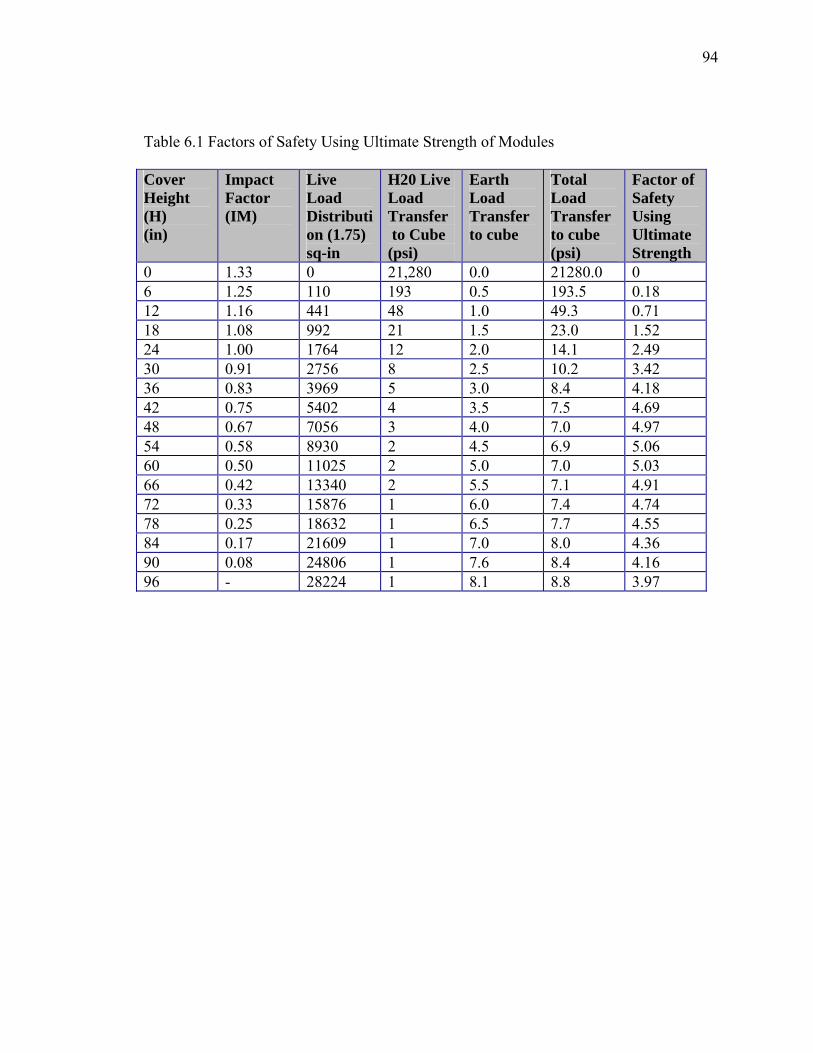
94
Table 6.1 Factors of Safety Using Ultimate Strength of Modules
Cover Height (H) (in)
Impact Factor (IM)
Live Load Distribution (1.75) sq-in
H20 Live Load Transfer to Cube (psi)
Earth Load Transfer to cube
Total Load Transfer to cube (psi)
Factor of Safety Using Ultimate Strength
0 1.33 0 21,280 0.0 21280.0 0 6 1.25 110 193 0.5 193.5 0.18 12 1.16 441 48 1.0 49.3 0.71 18 1.08 992 21 1.5 23.0 1.52 24 1.00 1764 12 2.0 14.1 2.49 30 0.91 2756 8 2.5 10.2 3.42 36 0.83 3969 5 3.0 8.4 4.18 42 0.75 5402 4 3.5 7.5 4.69 48 0.67 7056 3 4.0 7.0 4.97 54 0.58 8930 2 4.5 6.9 5.06 60 0.50 11025 2 5.0 7.0 5.03 66 0.42 13340 2 5.5 7.1 4.91 72 0.33 15876 1 6.0 7.4 4.74 78 0.25 18632 1 6.5 7.7 4.55 84 0.17 21609 1 7.0 8.0 4.36 90 0.08 24806 1 7.6 8.4 4.16 96 - 28224 1 8.1 8.8 3.97

95
Table 6.2 Factors of Safety Using Creep Yield Strengths
Cover Height (H) (in)
Impact Factor (IM)
Live Load Distribution (1.75)sq-in
H20 Live Load Transfer to Cube (psi)
Earth Load Transfer to cube (psi)
Total Load Transfer to cube (psi)
Factor of Safety using Yield Strength
0 1.33 0 21,280 - 21,280.0 0.0 6 1.25 243 87.4 0.5 87.9 0.1 12 1.16 973 21.9 1.0 22.9 0.4 18 1.08 2190 9.7 1.5 11.2 0.7 24 1.00 3894 5.5 2.0 7.5 1.1 30 0.91 6084 3.5 2.5 6.0 1.4 36 0.83 8761 2.4 3.0 5.4 1.5 42 0.75 11925 1.8 3.5 5.3 1.5 48 0.67 15575 1.4 4.0 5.4 1.5 54 0.58 19712 1.1 4.5 5.6 1.5 60 0.50 24336 0.9 5.0 5.9 1.4 66 0.42 29447 0.7 5.5 6.3 1.3 72 0.33 35044 0.6 6.0 6.6 1.2 78 0.25 41128 0.5 6.5 7.1 1.2 84 0.17 47699 0.4 7.0 7.5 1.1 90 0.08 54756 0.4 7.6 7.9 1.0 96 - 62300 0.3 8.1 8.4 1.0

96
Table 6.3 Factors of Safety Using Creep Reduced Strengths
Cover Height (H) (in)
Impact Factor (IM)
Live Load Distribution (1.75) sq-in
H20 Live Load Transfer to Cube (psi)
Earth Load Transfer to cube (psi)
Total Load Transfer to cube (psi)
FS Creep Reduced Yield Strength
0 1.33 0 21,280 - 21,280.0 0.0 6 1.25 243 87.4 0.5 87.9 0.1 12 1.16 973 21.9 1.0 22.9 0.3 18 1.08 2190 9.7 1.5 11.2 0.5 24 1.00 3894 5.5 2.0 7.5 0.8 30 0.91 6084 3.5 2.5 6.0 1.0 36 0.83 8761 2.4 3.0 5.4 1.1 42 0.75 11925 1.8 3.5 5.3 1.1 48 0.67 15575 1.4 4.0 5.4 1.1 54 0.58 19712 1.1 4.5 5.6 1.0 60 0.50 24336 0.9 5.0 5.9 1.0 66 0.42 29447 0.7 5.5 6.3 0.9 72 0.33 35044 0.6 6.0 6.6 0.9 78 0.25 41128 0.5 6.5 7.1 0.8 84 0.17 47699 0.4 7.0 7.5 0.8 90 0.08 54756 0.4 7.6 7.9 0.7 96 - 62300 0.3 8.1 8.4 0.7
To illustrate the previous tables of calculations, a graph is used to compare the FS values
calculated using ultimate strengths and varying thicknesses of cover soil to a creep
reduced curve using yield strength; see Figure 6.6.

97
Ultimate vs Yield vs Creep Reduced
-
1.0
2.0
3.0
4.0
5.0
6.0
0 6 12 18 24 30 36 42 48 54 60 66 72 78 84 90 96
Cover Soil Thickness (in)
F.S.
Ultimate Strength
Yield Strength
Creep Reduced
Fig. 6.6 Factor of Safety Values for Ultimate, Yield and Creep Reduced Strengths
The curves illustrate the vast differences in the FS values calculated based on
manufacture’s literature (ultimate strength) versus yield strength and long term design
strengths. Although the creep reduced strengths result in factors of safety close to 1.0 or
less, it can only be assumed that there have not been more failures due to H-20 loadings
not being applied consistently. The field conditions for parking lots are probably more
closely related to the yield strength curve.

98
CHAPTER 7. NANOCOMPOSITES USED WITH GEOSYNTHETICS
Polymers commonly used in producing geosynthetic materials include linear low density
polyethylene (LLDPE), high density polyethylene (HDPE), and polypropylene (PP).
These polymeric materials are viscoelastic and prone to creep. In applications such as
PSRM’s, an engineer is faced with balancing material costs versus performance. The
introduction of nanoclays to polymers, such as polyethylene, give the engineer the ability
to increase the durability with a relatively small increase in costs. This chapter will
review the manufacturing process as well as review of improvement to other physical
properties. Compared with regular plastics, nanocomposites offers much improved
properties that are critical to geosynthetic applications. These properties include tensile
and flexural properties, puncture resistance, thermal expansion, creep resistance, barrier
properties etc.
7.1 Nanocomposites
By definition, nanocomposites are nanomaterials that combine one or more separate
components in order to obtain the best properties of each component (composite). In a
nanocomposite, nanoparticles (clay, metal, carbon nanotubes) act as fillers in a matrix,
usually polymeric. For this thesis, nanoclay particles were chosen due to their relatively
low cost as an additive to polyethylene. Nanocomposites are prepared by dispersing a
smectite nanoclay into a host polymer, generally at low levels less than 10 by weight by
percent levels. This is illustrated in Figure 7.1

99
Fig. 7.1 Schematic of Nanocomposite Structure (Nanocor)
This process is also termed exfoliation. When a nanoclay is substantially dispersed it is
said to be exfoliated. Exfoliation is facilitated by surface compatibilization chemistry,
which expands the nanoclay platelets to the point where individual platelets can be
separated from one another by mechanical shear or heat of polymerization.
Nanocomposites can be created using both thermoplastic and thermoset polymers, and
the specific compatibilization chemistries designed and employed are necessarily a
function of the host polymer's unique chemical and physical characteristics. In some
cases, the final nanocomposite will be prepared in a reactor during the polymerization
stage. For other polymer systems, processes have been developed to incorporate nanomer
nanoclays into a hot-melt compounding operation. For the purpose of this thesis we are
looking at nanocomposites prepared with smectite nanoclays and incorporated into
polyethylene by hot-melt compounding.

100
In general, the addition of nanocomposites results in gains in gas barrier resistance, flame
resistance, structural strength, and thermal properties yet without significant loss in other
properties. Because of the nanometer sized dimensions of the individual platelets in one
direction, exfoliated nanomer nanoclays are transparent in most polymer systems.
However, with surface dimensions extending to one micron, the tightly bound structure in
a polymer matrix is impermeable to gases and liquids, and offers superior barrier
properties over the reference polymer. Nanocomposites also demonstrate enhanced fire
resistant properties and are finding increasing use in engineering plastics (Nanocor).
7.2 Nanoclay Structures
The essential nanoclay bare material is montmorillonite, a 2-to-1 layered smectite clay
mineral with a plate-like structure; see Figure 7.2. The bentonite familiar to most
geotechnical engineers is highly colloidal product of volcanic ash.
Fig. 7.2 Montmorillonite's unique structure creates a platey particle
Individual platelet thicknesses are just one nanometer (one-billionth of a meter), but
surface dimensions are generally 300 to more than 600 nanometers, resulting in an
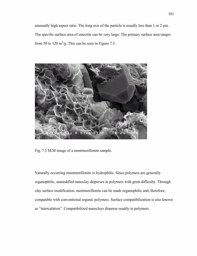
101
unusually high aspect ratio. The long axis of the particle is usually less than 1 or 2 μm.
The specific surface area of smectite can be very large. The primary surface area ranges
from 50 to 120 m2/g. This can be seen in Figure 7.3.
Fig. 7.3 SEM image of a montmorillonite sample.
Naturally occurring montmorillonite is hydrophilic. Since polymers are generally
organophilic, unmodified nanoclay disperses in polymers with great difficulty. Through
clay surface modification, montmorillonite can be made organophilic and, therefore,
compatible with conventional organic polymers. Surface compatibilization is also known
as “intercalation”. Compatibilized nanoclays disperse readily in polymers.

102
There are a number of chemistries to make a surface compatible for nanoclays. For
example, in addition to traditional onuim ion modification there has been a system
developed and patented a novel means for modification by leaving the sodium ion on the
surface and coordinating it via ion-dipole interaction. Regardless of the modification
technology used, the resulting clay-chemical complex, which exhibits a definite gallery
spacing between the platelets, is called a Nanomer nanoclay, and is supplied as a free-
flowing, micronized powder. When nanoclays are dispersed in a polymer matrix, they
form a near-molecular blend called a nanocomposite.
Polymer silicate nanocomposites incorporate layered clay mineral fillers in a polymer
matrix; see Figure 7.4.
Nanoclay Particles
Polyethylene
Fig. 7.4 Nanoclay Dispersed in Polyethylene

103
Layered silicates are made up of several hundred thin platelet layers stacked into an
orderly packet known as a tactoid. Each of these platelets is characterized by a large
aspect ratio (diameter/thickness on the order of 100-1000). Accordingly, when the clay is
dispersed homogeneously and exfoliated as individual platelets throughout the polymer
matrix, dramatic increases in strength, flexural modulus and Young’s modulus and heat
distortion temperature are observed at very low filler loadings (<10% by weight) because
of the large surface area contact between polymer and filler. In addition, barrier
properties are greatly improved because the large surface area of the platelets greatly
increased the tortuosity of the path a diffusing species must follow in permeating through
the polymeric materials. Ever since the initial development of Nylon 6, 6 nanocomposites
by Toyota research group in 1993, nanocomposites has been viewed as an effective way
to improve the performance of a variety of plastics without many property trade-offs.
7.3 Underground Water Storage System
Similarly, creep performance is a critical factor in designing underground storm water
storage system. Under sustained load from backfill and above ground structures or
automobiles, storage systems made of HDPE experiences deformation and drops of
effective modulus, which lead to collapses of the system and the ground above. Figure
7.5 illustrates this point, by showing the reduction in time to failure by increasing the
stress to strength ratio. To prevent this type of failure one would have to change to
stronger more expensive resin or find a HDPE resin with higher initial modulus and
higher creep resistance. One way to increase the tensile and flexural modulus of HDPE is
by the addition of relatively small amounts of nanoclay.

104
Fig. 7.5 Compression Creep for a Polyethylene Geonet (Narejo and Allen, 2010)
7.4 Nanocomposite Sample Preparation
Both samples of films and bar were prepared for testing. The films were produced using
an extruder (Figure 7.6) and bars made by producing a plaque.
Fig. 7.6 American Leistritz Extruder Model ZSE 27

105
Films and bars (Figure 7.7) were produced to test various properties.
(a) Nanocomposite films (b) Nanocomposite Bars
Fig. 7.7 Samples of Films and Bars with Varying Levels of Nanoclay
Fig. 7.8 Instron used for Tensile Testing

106
Fig. 7.9 Flexural Modulus Testing
7.5 Stepped Isothermal Method (SIM) Testing
One of the key long term design consideration for plastics is creep. Creep is a long term
phenomenon and its effect is based on the applied load and type of polymer. Plastics can
be put under constant load for 10,000 hours or constant rate of strain until failure. To test
a material for 10,000 hours in a laboratory would take over a year. If one wants to
accelerate the creep testing of a geosynthetics they can use a technique called the Stepped
Isothermal Method (SIM). ASTM D6992 describes the technique that "accelerates" the
creep by increasing the temperature in steps and then shifts the data using time-
temperature superpositioning principles to longer time periods. The SIM technique
allows for more than 10,000 hours of compressive creep to be simulated in less than 24
hours.
This is a valuable tool in evaluating long term compressive strength of geocomposite
drainage layers. For a three dimensional modular plastic cube supporting a pavement
section this long term compressive strength becomes even more important. Excessive

107
strains in the plastic modules will reflect through the overlying pavement. Therefore,
evaluating different polymers through the SIM test will give an indication of long term
performance.
7.6 LLDPE Nanocomposites
LLDPE nanocomposites with 3, 6 and 9% by weight of nanocomposites were prepared
by compounding LLDPE neat polymer and nanomasterbatch with a twin screw extruder.
The three samples are designated as LLDPE-3, LLDPE-6 and LLDPE-9, respectively.
The LLDPE sample without any nanocomposite was also included in the property studies
as control sample and is designated as LLDPE-C. The property studies of all four
samples are summarized in Table 7.1.
As shown in Table 7.1, the tensile modulus of LLDPE increased by 20% by incorporation
of 3% Nanocomposite. The puncture strength increased by more than 60% while
coefficient of thermal expansion dropped by 40%. More importantly, addition of the
nanocomposite greatly improved the creep resistance of LLDPE. The creep deformation
of LLDPE-9 at the end of 50 years is still smaller than the creep deformation of virgin
LDPE at 10,000 hours (about 1 year). In addition, the methane permeation through
membrane dropped by around 20%.

108
Table 7.1 Summary of Test Results of Linear Low Density Polyethylene Nanocomposites.
LDPE-C LDPE-3 LDPE-6 LDPE-9
Yield Strength (psi) 1662 1805 1881 1966Break Strength (psi) 4327 4316 4395 4367Yield Elongation (%) 20.5 20.4 19.5 19.2Break Elongation (%) 839 801 808 7960.02 Secant Modulus (psi) 44111 49188 53784 56173Young's Modulus (psi) 50153 61459 65157 62197
Puncture Strength (lbs) 31.7 49.9 50.3 54.4Displacement @ max load (inches) 1.09 1.05 1.02 1.00
CLTE (µm / m / ˚C) 172 109 85 83
Onset of Melt (˚C) 120.1 120 121.5 119.6Peak Melt (˚C) 123.9 124.5 124.1 123.9Heat of Fusion (J/g) 106.6 100.9 96.6 94.4
Strain at 10000 hours (%) 12.00 9.48 8.50 7.21Strain at 50 Years (%) 18.48 14.76 13.25 11.09
Permeation (cm2/sec-atm) 6.30E-08 5.20E-08 1.10E-08 1.00E-08Permeation [(cm3)(cm)/(cm2)(sec)(Pa)] 6.20E-13 5.10E-13 4.00E-13 3.90E-13
Tensile Properties - (ASTM D 6693 - 2ipm strain rate)
Methane Transmission (ASTM D 1434, Method V)
Puncture Properties (ASTM D 4833)
Coeff. Of Linear Thermal Expansion (ASTM D 696)
Melting Point - Differential Scanning Calorimetry (ASTM D 3418)
Time-Dependent Loading (ASTM D 6992 - Creep at 500 psi Stress)
7.7 HDPE Nanocomposites
HDPE nanocomposites with 3, 6 and 9% by weight of nanocomposite were prepared by
compounding HDPE neat polymer and nanomasterbatch with a twin screw extruder. The
three samples are designated as HDPE-3, HDPE-6 and HDPE-9, respectively. The HDPE
sample without any nanocomposite was also included in the property studies as control
sample and is designated as HDPE-C. The property studies of all four samples are
summarized in Table 7.2.

109
As shown in Table 7.2, the tensile modulus of HDPE increased by 10% by
incorporation of 3% nanocomposite. When 9% nanocomposite is loaded, the tensile
modulus increased by 60%. 10% to 35% decrease in creep deformation was achieved by
adding 3 to 9% nanocomposite. The deformation of the 9% sample at 50 years was
smaller than the deformation of virgin HDPE at 10,000 hours (about 1 year). Methane
permeation dropped by 50%.
Table 7.2 Summary of Test Results of High Density Polyethylene Nanocomposites.
HDPE-C HDPE-3 HDPE-6 HDPE-9
Yield Strength (psi) 2614 2832 3180 3477Break Strength (psi) 4587 4438 3997 2464Yield Elongation (%) 16.1 15.6 14.8 14.2Break Elongation (%) 789 784 744 4200.02 Secant Modulus (psi) 76445 85647 102280 112883Young's Modulus (psi) 84471 94725 122948 135214
Puncture Strength (lbs) 37.9 38.4 33.0 43.3Displacement @ max load (inches) 0.98 1.00 1.06 1.14
CLTE (µm / m / ˚C) 109 129 70 120
Onset of Melt (˚C) 119.5 120.3 120.5 121.1Peak Melt (˚C) 124.2 125 126 127.1Heat of Fusion (J/g) 142.8 158.2 157.8 159.3
Strain at 10000 hours (%) 2.83 2.50 1.88 1.81Strain at 50 Years (%) 3.42 2.99 2.32 2.26
Permeation (cm2/sec-atm) 3.30E-08 2.00E-08 1.70E-08 1.60E-08Permeation [(cm3)(cm)/(cm2)(sec)(Pa)] 3.20E-13 2.00E-13 1.70E-13 1.60E-13
Methane Transmission (ASTM D 1434, Method V)
Puncture Properties (ASTM D 4833)
Tensile Properties - (ASTM D 6693 - 2ipm strain rate)
Coeff. Of Linear Thermal Expansion (ASTM D 696)
Melting Point - Differential Scanning Calorimetry (ASTM D 3418)
Time-Dependent Loading (ASTM D 6992 - Creep at 500 psi Stress)

110
In summary, compared to virgin LLDPE and HDPE, the nanocomposites offer a tougher
material with better dimension stability at high temperature or under high stress. The
nanocomposites also provide better barrier properties against methane and other organic
vapor. Unlike traditional composite materials, nanocomposites offer the significant
property improvement with only ~5% Nanocomposite loading, which means the density
and thermal flow properties remain similar to virgin plastics. Therefore, nanocomposites
can be used as a “drop in” material to most existing manufacture lines.
7.8 Environmental Stress Cracking
Environmental stress cracking is the formation of cracks in a material caused by
relatively low tensile stress and environmental conditions. Environmental Stress-
Cracking Resistance (ESCR) is the number of hours that 50% of the specimens tested
exhibit stress cracks. The standardized test to evaluate ESCR is ASTM D1693. Testing is
performed by slowly bending the test specimens and placing them in a holding clamp.
The clamp and specimens are then placed in a test tube and immersed in a specified
reagent. The test tube is sealed and placed in a constant-temperature bath. Multiple test
specimens are tested at one time
Test results ESCR using ASTM D 1693 are shown in Table 7.3.

111
Table 7.3 ESCR Test Results using ASTM D1693 (Nanocor) ESCR (hours)
Control 42
3 % Nanoclay 94
6% Nanoclay 141
The preferred test method to evaluate stress cracking is ASTM D5397. This test method
is intended as an index test and may be used for grading polyolefin geomembrane sheets
in regard to their stress cracking sensitivity.
7.9 Creep Strain
In addition to the improved physical properties, nanocomposites also reduce the amount
of creep strain. The following four figures percent graph strain versus time under a 500
psi load for various loadings of nanoclay.

112
Fig. 7.10 SIM of Control sample, no Nanoclay % Strain versus Log
Time (HR) (TRI Data)
Fig. 7.11 SIM on Sample with 3% Nanoclay, Strain versus
Log Time (HR) (TRI Data)
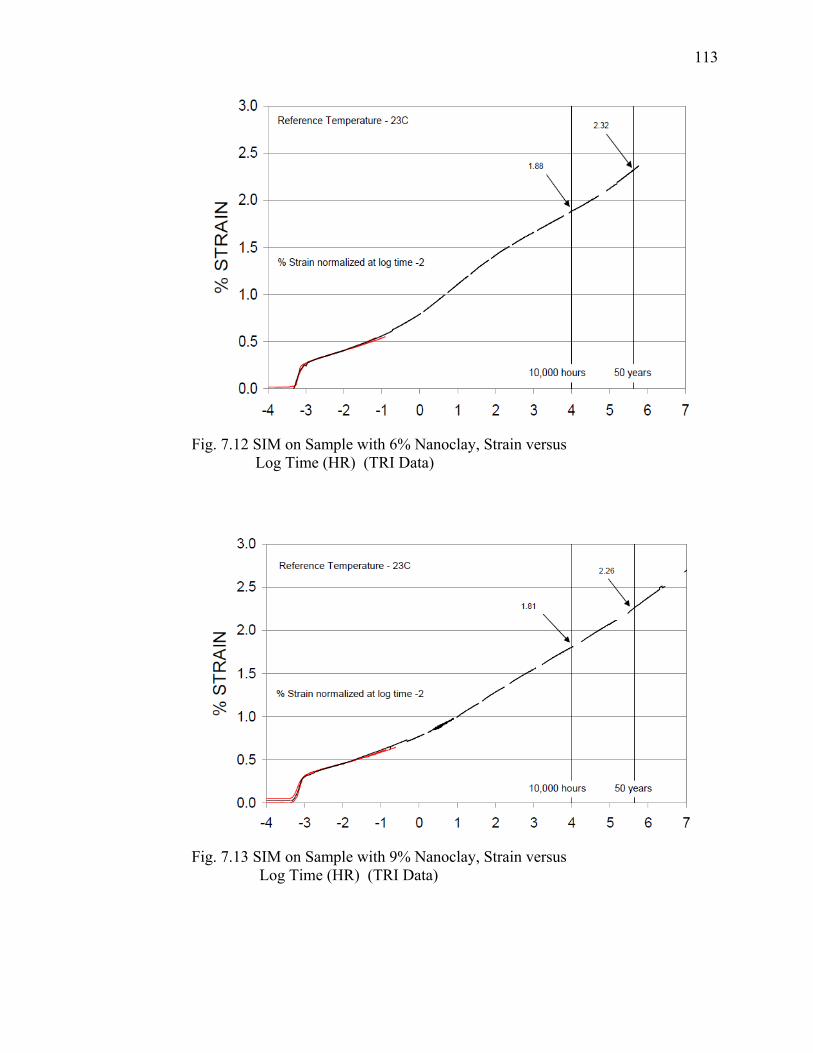
113
Fig. 7.12 SIM on Sample with 6% Nanoclay, Strain versus
Log Time (HR) (TRI Data)
Fig. 7.13 SIM on Sample with 9% Nanoclay, Strain versus
Log Time (HR) (TRI Data)

114
7.10 HDPE Nanocomposites from Recycled HDPE
Sustainability has become a major drive towards better recycling, reduced carbon
footprint and renewable sources. HDPE is one of the most-often recycled plastics.
However, the properties of recycled HDPE are inferior compared with virgin HDPE due
to the oxidative and photo degradations in its use life. This property degradation has
partially limited the use of recycled HDPE in geosynthetic applications. By the same
principle for property improvement by nanocomposites, we have shown that the property
of recycled HDPE can be improved to and above those of virgin HDPE.
In this study, virgin HDPE was compounded three times to mimic property degradation
of recycled plastics. Virgin HDPE was designated as HDPE-0, with the samples from
additional compounding step were designated as HDPE-1, HDPE-2 and HDPE-3
respectively. HDPE-3 was made in nanocomposites with 3, 6 and 9 weight percentage of
clay and the samples were designated as HDPE-3+3% clay, HDPE-3+6% clay and
HDPE-3+9% clay. The tensile and flexural properties of all samples were studied and
plotted in Figures 7.14 and 7.15.
As shown in Figure 7.14, the tensile strength of HDPE dropped by around 3% after being
compounded three times (HDPE-3 vs. HDPE-0). With 3% clay loading, the tensile
strength restored to the level of virgin HDPE. With 6 and 9% clay loading, the tensile
strength of the nanocomposites exceeded the value of the virgin HDPE. The same trend
was observed in the flexural strength in Figure 7.15.

115
3500
3600
3700
3800
3900
4000
4100
HDPE-0 HDPE-1 HDPE-2 HDPE-3 HDPE-3+3% clay
HDPE-3+6% clay
HDPE-3+9% clay
Tens
ile Y
ield
Stre
ngt
(psi)
-6
-5
-4
-3
-2
-1
0
1
2
3
%ch
ange
Tensile Yield Strength %Change
Fig. 7.14 Tensile Property Degradation by Repeated Compounding and Restoration by Nanocomposites.
3800
3900
4000
4100
4200
4300
4400
4500
4600
HDPE-0 HDPE-1 HDPE-2 HDPE-3 HDPE-3+3% clay
HDPE-3+6% clay
HDPE-3+9% clay
Flex
ural
Yie
ld S
treng
t(p
si)
-6
-4
-2
0
2
4
6
8
%ch
ange
Flexural Yield Strength %Change
Fig. 7.15 Flexural Property Degradation by Repeated Compounding and Restoration by Nanocomposites.
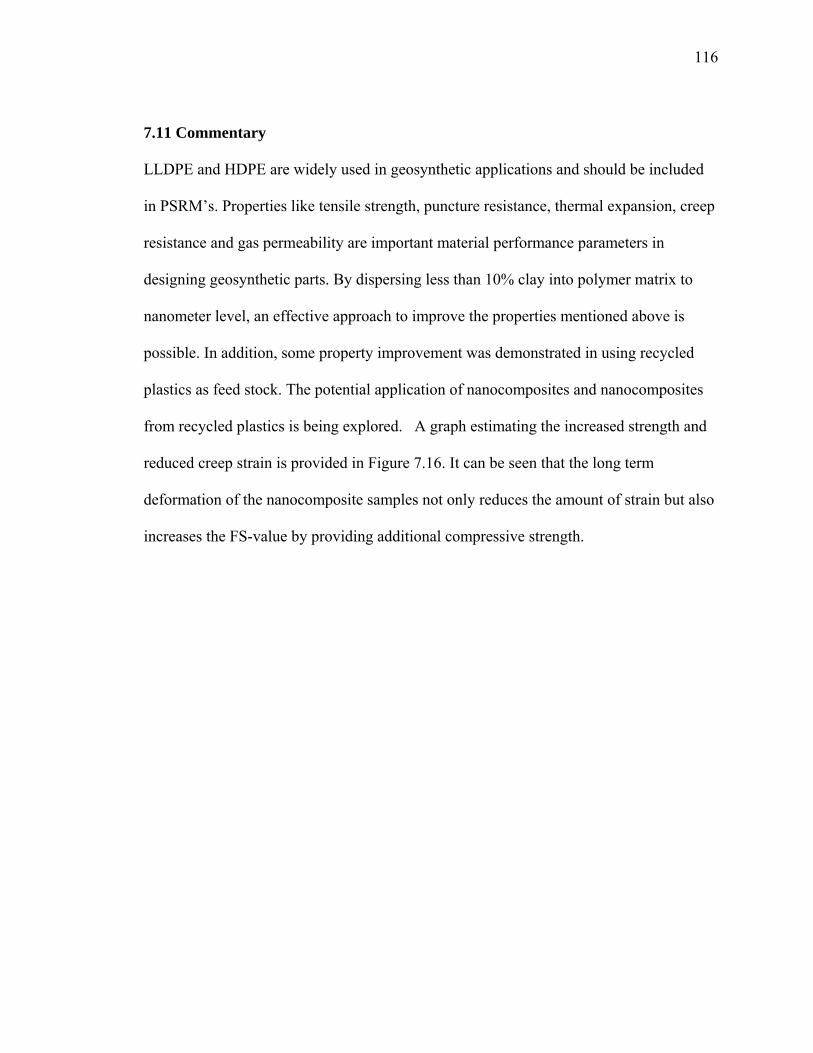
116
7.11 Commentary
LLDPE and HDPE are widely used in geosynthetic applications and should be included
in PSRM’s. Properties like tensile strength, puncture resistance, thermal expansion, creep
resistance and gas permeability are important material performance parameters in
designing geosynthetic parts. By dispersing less than 10% clay into polymer matrix to
nanometer level, an effective approach to improve the properties mentioned above is
possible. In addition, some property improvement was demonstrated in using recycled
plastics as feed stock. The potential application of nanocomposites and nanocomposites
from recycled plastics is being explored. A graph estimating the increased strength and
reduced creep strain is provided in Figure 7.16. It can be seen that the long term
deformation of the nanocomposite samples not only reduces the amount of strain but also
increases the FS-value by providing additional compressive strength.

117
Stress - Compression
0
1,000
2,000
3,000
4,000
5,000
6,000
7,000
8,000
9,000
0 0.2 0.4 0.6 0.8 1 1.2
in
lbf
0.247 0.270 0.378
NanoComposite As received
Creep reduced
Additional FS
Fig. 7.16 Comparison of Expected Stress Strain Curves for Plastic Modules as Currently Received, Creep Reduced and with Nanocomposites

118
CHAPTER 8. CONCLUSIONS AND RECOMMENDATIONS This chapter summarizes the assumptions made at the beginning of this thesis and
compares them to the results of material testing of the PSRM’s. In addition to confirming
concerns regarding long term durability of these systems, this chapter offers a process to
improve the long term performance using nanoclays and offers suggestions on tests
methods, raw material selection and future research.
8.1 Summary
As stormwater regulations continue to increase throughout the USA there will be an
increasing need to cost effectively store the stormwater captured from building sites. As
the market for stormwater retention increases, so will the number of manufacturers who
product various stormwater management systems. As with most markets the increased
competition will drive the systems to be more cost effective and will result in lower
weight and possibly inferior products. As a result there should be a testing standard
available such as ASTM to establish minimum strengths and requirements for these
systems. A draft has been provided in an Appendix A, as well as a specification of
minimum values.
An assumption made at the beginning of this thesis was that most manufacturers are
reporting the ultimate strength of their products and using that value for the long term
design strengths and factor of safety calculations. The testing completed within this thesis
proved this to be true. As with any construction material, design strengths of materials

119
should be within the yield strength or elastic region of the stress strain curve. The yield
strength in some cases is almost half of the ultimate strength.
In addition to the ultimate strength reported as a design value, there is no consideration
for the long term creep strength of the plastic modules. These materials are all made from
viscoelastic plastics and can be greatly effected be creep dependent on the load applied to
them during their service life.
Long term creep strength of strengths within the elastic region must be used for design
purposes in order to report a reliable long term design FS-values. There are well defined
design calculations for designing with geosynthetics, Koerner, 2005. The design
equations include reduction factors for creep (dependent of type of polymer). There are
also long term compressive strengths used for drainage composites that are tested for site
specific conditions. These methods could easily be adjusted to design for three
dimensional plastic stormwater modules.
Flexible pavement designs are based on limiting the amount of deflection transferred
from subgrade up to the wearing course. Stress versus strain curves must be provided to
design engineers in order to evaluate the amount of expected deflection in the pavement
system. To date, most manufactures only report strengths and no limiting strains or
modulus values. It has been shown that the amount of strain is dependent on the load
transferred to the PSRM and that is dependent on the depth of the system.

120
As with all other geosynthetics, there is a set manufacturing QA/QC plan that discusses
selection of raw materials prior to manufacturing as well as index tests to assure that all
materials used to produce a certain product meet minimum requirements. Many of these
products use recycled plastics and there needs to be better control over the source and
reliability of these materials. A good MQC/MQA plan would certainly be the way to
ensure reliable material sources.
The use of nanocomposite greatly increases the strength and long term design of
polyethylene products like PSRM’s. The addition of relatively small amounts of nanoclay
(3% - 9%) can produce large increases in modulus, flexural modulus and environmental
stress cracking resistance. In addition to increased strength, the same nanoclay decreases
the amount of creep strain. The combination of these attributes results in a much stronger
material with longer design life and/or higher factors of safety.
The use of nanoclay has the same effect on recycled plastics. In some cases, the
nanocomposite material made with recycled content has a higher strength the virgin
material itself. This is an asset when it comes to beneficial reuse of plastics and
sustainable material designs.

121
Future Research
The testing conducted in this thesis was for a single unit. In many cases these plastic
modules are stacked on top of each other to heights greater than seven feet as shown in
the Long Island, NY project. Full scale filed testing of these systems should be evaluated.
There is also a need to know how the flexing in an individual module is translated
through several modules when stacked on top of each other.
Nanoclays have shown to greatly improve the performance of polyethylene but little is
know about long term compatibility of these materials. Most of the testing reported in
this thesis show improvement to all the physical properties but there effects on other
additives should be evaluated.
The nanocomposite testing was performed on materials samples of films and bars
produced in a lab. The next step in process would be to produce full scale products and
test them side by side to the same product without nanoclay

122
List of References
1. Robert M. Koerner “Designing with Geosynthetics”, Prentice Hall 2005, 408-414
2. R. Veldhuijzen Van Zanten “Geotextiles and Geomembrnaes in Civil Engineering”, John Wiley & Sons, 144-160
3. R.J. Young and P.A. Lovell “Introduction to Polymers”, Chapman and Hall 1981;
4. D.H. Morton-Jones “Polymer Processing”, Chapman and Hall 1989, 6-37
5. G.R. Moore and D.E. Kline “Properties and Processing of Polymers for
Engineers”, Prentice-Hall 1984, 23-67
6. Domasius Nwabunma and Thein Kyu “Polyolefin Composites”, Wiley 2008, 251-275
7. E.J. Yoder and M.W. Witczak “ Principles of Pavement Desigh”, John Wiley &
Sons 1975
8. P. Wright and K. Dixon, “Highway Engineering” John Wiley & Sons, 2004
9. American Iron and Steel Institute, “Handbook of Steel Drainage & Highway Construction Products”, W.P. Reyman Associates, 1983
10. C.S. Papacostas and P.D. Prevedouros, “transpostation Engineering & Planning”,
Prentice Hall, 2001
11. Norman E. Dowling “Mechanical Behavior of Materials” Prentice Hall 2007; 171-185
12. James K. Mitchell and Kenichi Soga, “Fundementals of Soil Behavior” Wiley,
2005; 52-65
13. Arthur P. Boresi and Richard J. Schmidt, “Advanced Mechanics of Materials” Wiley, 2003; 5-22
14. Design Computations for: CUDO Water Storage System, Terrain Engineering
Inc. 2008
15. Stephen Fenichell, “Plastic: The Making of a Synthetic Century”, 1996, p. 17

123
16. ASTM D 4632, 2008. Standard Test Method for Grab Breaking Load and Elongation of Geotextiles. American Society for Testing and materials, West Conshocken, Pennsylvania, USA
17. ASTM D 6364, 2006. Standard Test Method Determining Short-Term
Compression Behavior of Geosynthetics, West Conshocken, Pennsylvania, USA
18. ASTM D 2412, 2002. Standard Test Method for Determination of Extrenal Loading Characteristics of Plastic Pipe by Parallel-Plate Loading, West Conshocken, Pennsylvania, USA
19. Robert M. Koerner, GSI White Paper #4, Reduction Factors (RFs) Used in
Geosynthetic Design, Geosynthetic Institute
20. Robert M. Koerner, GSI White Paper #6, Reduction Factors (RFs) Used in Geosynthetic Design, Geosynthetic Institute

124
APPENDIX A

TRI / Environmental, Inc. A Texas Research International Company
CETCO Contracting Services CompanyThin Film Comparison Study - Summary of Test Results
LD-C LD-3 LD-6 LD-9 HD-C HD-3 HD-6 HD-9Tensile Properties - from film (ASTM D 6693 - 2ipm strain rate)
MD Yield Strength (psi) 1400 1711 1787 1864 2227 2727 2824 3299TD Yield Strength (psi) 1381 1698 1744 1897 2316 2781 3103 3283
MD Break Strength (psi) 4574 4829 4846 4918 4081 4319 4385 4562TD Break Strength (psi) 5208 5011 5057 4869 4829 5011 5086 4796
MD Yield Elongation (%) 18.3 20.2 20.1 21.4 14.7 18.7 19.2 15.8TD Yield Elongation (%) 16.2 19.8 19.2 18.9 17.2 18.6 18.2 18.1
MD Break Elongation (%) 867 896 878 903 558 598 549 643TD Break Elongation (%) 999 909 914 930 762 748 700 802
Tensile Properties - from compression molded plaques (ASTM D 6693 - 2 ipm strain rate)
Yield Strength (psi) 1662 1805 1881 1966 2614 2832 3180 3477Break Strength (psi) 4327 4316 4395 4367 4587 4438 3997 2464Yield Elongation (%) 20.5 20.4 19.5 19.2 16.1 15.6 14.8 14.2Break Elongation (%) 839 801 808 796 789 784 744 4202% Secant Modulus (psi) 44111 49188 53784 56173 76445 85647 102280 112883Young's Modulus (psi) 50153 61459 65157 62197 84471 94725 122948 135214
Puncture Properties (ASTM Dc 4833)
Puncture Strength (lbs) 31.7 49.9 50.3 54.4 37.9 38.4 33.0 43.3Displacement @ max load (inches) 1.09 1.05 1.02 1.00 0.98 1.00 1.06 1.14
Coeff. Of Linear Thermal Expansion (ASTM D 696)
CLTE (µm / m / OC) - 10g - plaque 173 222 189 261 173 170 218 210CLTE (µm / m / OC) - 5g - film 172 109 85 83 109 129 70 120
Melting Point - Differential Scanning Calorimetry (ASTM D 3418)
Onset of Melt (OC) - FIRST HEAT 118.3 116.9 118.3 118.1 117.0 118.1 119.5 120.8Onset of Melt (OC) - SECOND HEAT 120.1 120.0 121.5 119.6 119.5 120.3 120.5 121.1
Peak Melt (OC) - FIRST HEAT 123.8 125.1 124.5 124.5 123.3 124.1 125.1 126.1Peak Melt (OC) - SECOND HEAT 123.9 124.5 124.1 123.9 124.2 125.0 126.0 127.1
Heat of Fusion (J/g) - FIRST HEAT 105.9 95.5 93.7 91.5 132.7 148.8 143.4 145.3Heat of Fusion (J/g) - SECOND HEAT 106.6 100.9 96.6 94.4 142.8 158.2 157.8 159.3
Time-Dependent Loading (ASTM D 6992 - Creep at 500 psi Stress) - from compression molded plaques
Strain at 10,000 hours (%) 12.00 9.48 8.50 7.21 2.83 2.50 1.88 1.81Strain at 50 Years (%) 18.48 14.76 13.25 11.09 3.42 2.99 2.32 2.26
Methane Transmission (ASTM D 1434, Method V)
Permeation (cm2/sec-atm) 6.3E-08 5.2E-08 1.1E-08 1.0E-08 3.3E-08 2.0E-08 1.7E-08 1.6E-08Permeation [(cm3)(cm)/(cm2)(sec)(Pa)] 6.2E-13 5.1E-13 4.0E-13 3.9E-13 3.2E-13 2.0E-13 1.7E-13 1.6E-13
DP-Data PendingNOTES:
Surface blemishes and localized out-of-plane deformations were observed on provided samples. In addition, initial thermal testing revealed various levels of residual stresses. For these reasons, compression molded plaques were manufactured from provided samples., then used to test coefficient of thermal expansion (CLTE), repetitive tensile properties, and time dependent strain properties using the Stepped Isothermal Method (SIM).
The thermal transition temperatures of each sample were measured in accordance with ASTM D 3418. An initial heat was performed to remove residual stresses. A second programmed heat was performed to determine test results.
9063 Bee Caves Road / Austin, TX 78733 / 512 263 2101 / fax: 512 263 2558 / www.GeosyntheticTesting.com
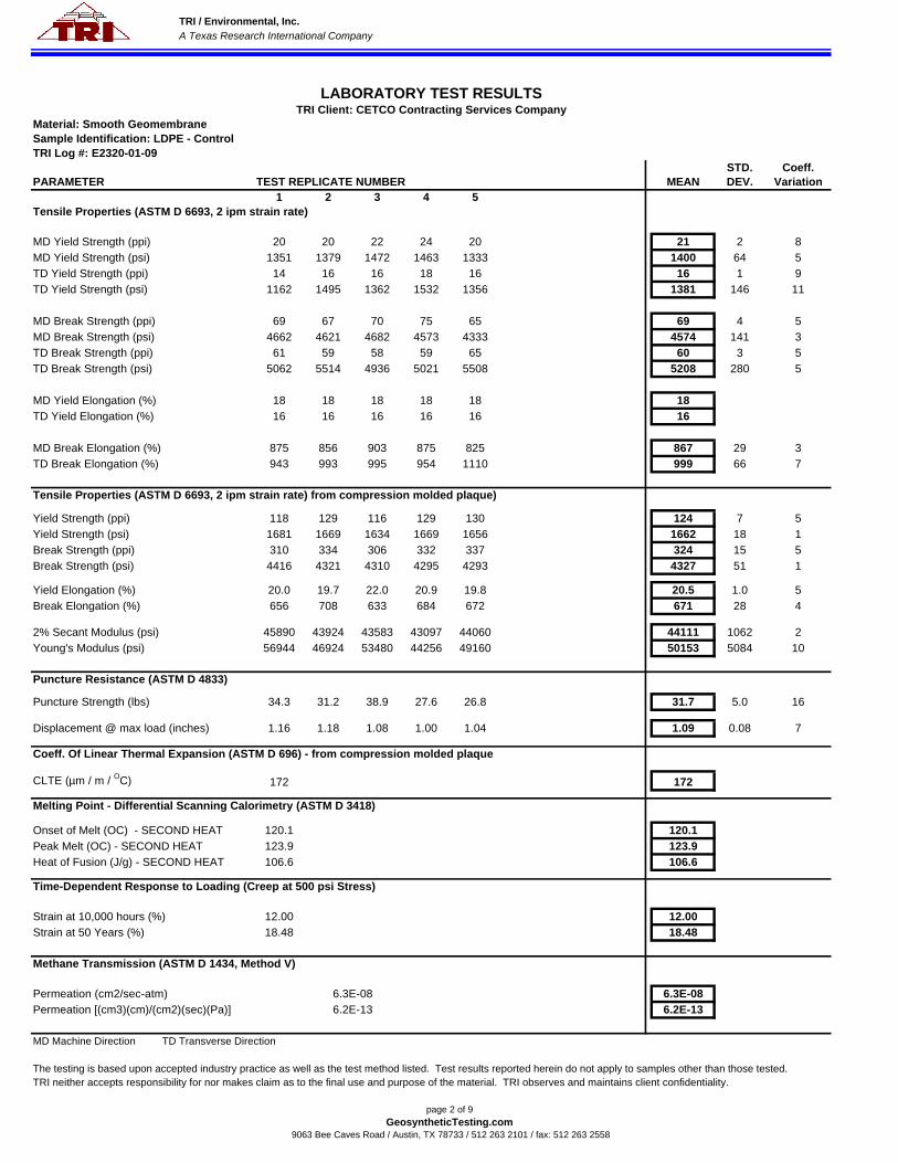
TRI / Environmental, Inc. A Texas Research International Company
LABORATORY TEST RESULTSTRI Client: CETCO Contracting Services Company
Material: Smooth GeomembraneSample Identification: LDPE - ControlTRI Log #: E2320-01-09
STD. Coeff.PARAMETER TEST REPLICATE NUMBER MEAN DEV. Variation
1 2 3 4 5Tensile Properties (ASTM D 6693, 2 ipm strain rate)
MD Yield Strength (ppi) 20 20 22 24 20 21 2 8MD Yield Strength (psi) 1351 1379 1472 1463 1333 1400 64 5TD Yield Strength (ppi) 14 16 16 18 16 16 1 9TD Yield Strength (psi) 1162 1495 1362 1532 1356 1381 146 11
MD Break Strength (ppi) 69 67 70 75 65 69 4 5MD Break Strength (psi) 4662 4621 4682 4573 4333 4574 141 3TD Break Strength (ppi) 61 59 58 59 65 60 3 5TD Break Strength (psi) 5062 5514 4936 5021 5508 5208 280 5
MD Yield Elongation (%) 18 18 18 18 18 18TD Yield Elongation (%) 16 16 16 16 16 16
MD Break Elongation (%) 875 856 903 875 825 867 29 3TD Break Elongation (%) 943 993 995 954 1110 999 66 7
Tensile Properties (ASTM D 6693, 2 ipm strain rate) from compression molded plaque)
Yield Strength (ppi) 118 129 116 129 130 124 7 5Yield Strength (psi) 1681 1669 1634 1669 1656 1662 18 1Break Strength (ppi) 310 334 306 332 337 324 15 5Break Strength (psi) 4416 4321 4310 4295 4293 4327 51 1
Yield Elongation (%) 20.0 19.7 22.0 20.9 19.8 20.5 1.0 5Break Elongation (%) 656 708 633 684 672 671 28 4
2% Secant Modulus (psi) 45890 43924 43583 43097 44060 44111 1062 2Young's Modulus (psi) 56944 46924 53480 44256 49160 50153 5084 10
Puncture Resistance (ASTM D 4833)
Puncture Strength (lbs) 34.3 31.2 38.9 27.6 26.8 31.7 5.0 16
Displacement @ max load (inches) 1.16 1.18 1.08 1.00 1.04 1.09 0.08 7
Coeff. Of Linear Thermal Expansion (ASTM D 696) - from compression molded plaque
CLTE (µm / m / OC) 172 172
Melting Point - Differential Scanning Calorimetry (ASTM D 3418)
Onset of Melt (OC) - SECOND HEAT 120.1 120.1Peak Melt (OC) - SECOND HEAT 123.9 123.9Heat of Fusion (J/g) - SECOND HEAT 106.6 106.6
Time-Dependent Response to Loading (Creep at 500 psi Stress)
Strain at 10,000 hours (%) 12.00 12.00Strain at 50 Years (%) 18.48 18.48
Methane Transmission (ASTM D 1434, Method V)
Permeation (cm2/sec-atm) 6.3E-08Permeation [(cm3)(cm)/(cm2)(sec)(Pa)] 6.2E-13
MD Machine Direction TD Transverse Direction
The testing is based upon accepted industry practice as well as the test method listed. Test results reported herein do not apply to samples other than those tested.TRI neither accepts responsibility for nor makes claim as to the final use and purpose of the material. TRI observes and maintains client confidentiality.
6.3E-086.2E-13
page 2 of 9GeosyntheticTesting.com
9063 Bee Caves Road / Austin, TX 78733 / 512 263 2101 / fax: 512 263 2558

TRI / Environmental, Inc. A Texas Research International Company
LABORATORY TEST RESULTSTRI Client: CETCO Contracting Services Company
Material: Smooth GeomembraneSample Identification: LDPE - 3TRI Log #: E2320-01-09
STD. PROJ.PARAMETER TEST REPLICATE NUMBER MEAN DEV. SPEC.
1 2 3 4 5 6 7 8 9 10Tensile Properties (ASTM D 6693, 2 ipm strain rate)
MD Yield Strength (ppi) 33 34 34 34 35 34 1 2MD Yield Strength (psi) 1692 1704 1667 1671 1823 1711 64 4TD Yield Strength (ppi) 34 34 34 35 36 35 1 3TD Yield Strength (psi) 1700 1700 1679 1687 1722 1698 17 1
MD Break Strength (ppi) 93 93 101 98 95 96 3 4MD Break Strength (psi) 4769 4662 4951 4816 4948 4829 123 3TD Break Strength (ppi) 105 108 107 83 107 102 11 10TD Break Strength (psi) 5250 5400 5284 4000 5120 5011 574 11
MD Yield Elongation (%) 20 19 20 20 20 20TD Yield Elongation (%) 20 20 20 20 20 20
MD Break Elongation (%) 866 836 928 931 916 896 42 5TD Break Elongation (%) 963 1005 959 709 911 909 117 13
Tensile Properties (ASTM D 6693, 2 ipm strain rate) from compression molded plaque)
Yield Strength (ppi) 131 132 130 134 131 132 2 1Yield Strength (psi) 1812 1767 1816 1826 1804 1805 22 1Break Strength (ppi) 315 312 323 310 313 315 5 2Break Strength (psi) 4357 4177 4511 4223 4311 4316 130 3
Yield Elongation (%) 20.8 19.7 21.4 19.8 20.2 20.4 0.7 4Break Elongation (%) 645 625 654 631 648 641 12 2
2% Secant Modulus (psi) 49424 50548 46683 50505 48782 49188 1587 3Young's Modulus (psi) 64477 76916 57254 56370 52276 61459 9695 16
Puncture Resistance (ASTM D 4833)
Puncture Strength (lbs) 53.6 49.4 48.3 49.0 49.1 49.9 2.1 4
Displacement @ max load (inches) 1.06 1.06 1.04 1.04 1.04 1.05 0.01 1
Coeff. Of Linear Thermal Expansion (ASTM D 696)
CLTE (µm / m / OC) 109 109
Melting Point - Differential Scanning Calorimetry (ASTM D 3418)
Onset of Melt (OC) - SECOND HEAT 120.0 120.0Peak Melt (OC) - SECOND HEAT 124.5 124.5Heat of Fusion (J/g) - SECOND HEAT 100.9 100.9
Time-Dependent Response to Loading (Creep at 500 psi Stress)
Strain at 10,000 hours (%) 9.48 9.48Strain at 50 Years (%) 14.76 14.76
Methane Transmission (ASTM D 1434, Method V)
Permeation (cm2/sec-atm) 5.2E-08Permeation [(cm3)(cm)/(cm2)(sec)(Pa)] 5.1E-13
MD Machine Direction TD Transverse Direction
The testing is based upon accepted industry practice as well as the test method listed. Test results reported herein do not apply to samples other than those tested.TRI neither accepts responsibility for nor makes claim as to the final use and purpose of the material. TRI observes and maintains client confidentiality.
5.1E-135.2E-08
page 3 of 9GeosyntheticTesting.com
9063 Bee Caves Road / Austin, TX 78733 / 512 263 2101 / fax: 512 263 2558
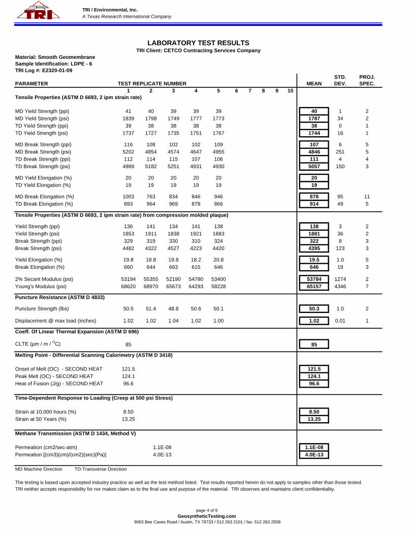
TRI / Environmental, Inc. A Texas Research International Company
LABORATORY TEST RESULTSTRI Client: CETCO Contracting Services Company
Material: Smooth GeomembraneSample Identification: LDPE - 6TRI Log #: E2320-01-09
STD. PROJ.PARAMETER TEST REPLICATE NUMBER MEAN DEV. SPEC.
1 2 3 4 5 6 7 8 9 10Tensile Properties (ASTM D 6693, 2 ipm strain rate)
MD Yield Strength (ppi) 41 40 39 39 39 40 1 2MD Yield Strength (psi) 1839 1798 1749 1777 1773 1787 34 2TD Yield Strength (ppi) 39 38 38 38 38 38 0 1TD Yield Strength (psi) 1737 1727 1735 1751 1767 1744 16 1
MD Break Strength (ppi) 116 108 102 102 109 107 6 5MD Break Strength (psi) 5202 4854 4574 4647 4955 4846 251 5TD Break Strength (ppi) 112 114 115 107 106 111 4 4TD Break Strength (psi) 4989 5182 5251 4931 4930 5057 150 3
MD Yield Elongation (%) 20 20 20 20 20 20TD Yield Elongation (%) 19 19 19 19 19 19
MD Break Elongation (%) 1003 763 834 846 946 878 95 11TD Break Elongation (%) 893 964 969 878 866 914 49 5
Tensile Properties (ASTM D 6693, 2 ipm strain rate) from compression molded plaque)
Yield Strength (ppi) 136 141 134 141 138 138 3 2Yield Strength (psi) 1853 1911 1838 1921 1883 1881 36 2Break Strength (ppi) 329 319 330 310 324 322 8 3Break Strength (psi) 4482 4322 4527 4223 4420 4395 123 3
Yield Elongation (%) 19.8 18.8 19.8 18.2 20.8 19.5 1.0 5Break Elongation (%) 660 644 663 615 646 646 19 3
2% Secant Modulus (psi) 53194 55355 52190 54780 53400 53784 1274 2Young's Modulus (psi) 68620 68970 65673 64293 58228 65157 4346 7
Puncture Resistance (ASTM D 4833)
Puncture Strength (lbs) 50.5 51.4 48.8 50.6 50.1 50.3 1.0 2
Displacement @ max load (inches) 1.02 1.02 1.04 1.02 1.00 1.02 0.01 1
Coeff. Of Linear Thermal Expansion (ASTM D 696)
CLTE (µm / m / OC) 85 85
Melting Point - Differential Scanning Calorimetry (ASTM D 3418)
Onset of Melt (OC) - SECOND HEAT 121.5 121.5Peak Melt (OC) - SECOND HEAT 124.1 124.1Heat of Fusion (J/g) - SECOND HEAT 96.6 96.6
Time-Dependent Response to Loading (Creep at 500 psi Stress)
Strain at 10,000 hours (%) 8.50 8.50Strain at 50 Years (%) 13.25 13.25
Methane Transmission (ASTM D 1434, Method V)
Permeation (cm2/sec-atm) 1.1E-08Permeation [(cm3)(cm)/(cm2)(sec)(Pa)] 4.0E-13
MD Machine Direction TD Transverse Direction
The testing is based upon accepted industry practice as well as the test method listed. Test results reported herein do not apply to samples other than those tested.TRI neither accepts responsibility for nor makes claim as to the final use and purpose of the material. TRI observes and maintains client confidentiality.
1.1E-084.0E-13
page 4 of 9GeosyntheticTesting.com
9063 Bee Caves Road / Austin, TX 78733 / 512 263 2101 / fax: 512 263 2558

TRI / Environmental, Inc. A Texas Research International Company
LABORATORY TEST RESULTSTRI Client: CETCO Contracting Services Company
Material: Smooth GeomembraneSample Identification: LDPE - 9TRI Log #: E2320-01-09
STD. PROJ.PARAMETER TEST REPLICATE NUMBER MEAN DEV. SPEC.
1 2 3 4 5 6 7 8 9 10Tensile Properties (ASTM D 6693, 2 ipm strain rate)
MD Yield Strength (ppi) 48 43 45 45 45 45 2 4MD Yield Strength (psi) 1857 1853 1848 1879 1883 1864 16 1TD Yield Strength (ppi) 46 45 45 45 45 45 0 1TD Yield Strength (psi) 1921 1867 1899 1883 1915 1897 22 1
MD Break Strength (ppi) 123 116 122 116 119 119 3 3MD Break Strength (psi) 4758 5000 5010 4843 4979 4918 112 2TD Break Strength (ppi) 102 119 113 122 124 116 9 8TD Break Strength (psi) 4259 4938 4768 5105 5277 4869 390 8
MD Yield Elongation (%) 21 21 21 21 21 21TD Yield Elongation (%) 19 19 19 19 19 19
MD Break Elongation (%) 881 900 950 884 898 903 28 3TD Break Elongation (%) 748 963 901 1018 1019 930 113 12
Tensile Properties (ASTM D 6693, 2 ipm strain rate) from compression molded plaque)
Yield Strength (ppi) 140 146 135 145 143 142 4 3Yield Strength (psi) 1966 2031 1878 1989 1964 1966 56 3Break Strength (ppi) 316 316 307 315 321 315 5 2Break Strength (psi) 4438 4395 4270 4321 4409 4367 69 2
Yield Elongation (%) 19.6 18.2 20.0 18.3 19.7 19.2 0.8 4Break Elongation (%) 646 624 635 625 654 637 13 2
2% Secant Modulus (psi) 55082 59550 53521 58187 54526 56173 2569 5Young's Modulus (psi) 59599 65553 59233 63916 62686 62197 2738 4
Puncture Resistance (ASTM D 4833)
Puncture Strength (lbs) 54.7 55.0 56.0 55.6 50.6 54.4 2.2 4
Displacement @ max load (inches) 1.04 1.02 1.02 1.02 0.92 1.00 0.05 5
Coeff. Of Linear Thermal Expansion (ASTM D 696)
CLTE (µm / m / OC) 83 83
Melting Point - Differential Scanning Calorimetry (ASTM D 3418)
Onset of Melt (OC) - SECOND HEAT 119.6 119.6Peak Melt (OC) - SECOND HEAT 123.9 123.9Heat of Fusion (J/g) - SECOND HEAT 94.4 94.4
Time-Dependent Response to Loading (Creep at 500 psi Stress)
Strain at 10,000 hours (%) 7.21 7.21Strain at 50 Years (%) 11.09 11.09
Methane Transmission (ASTM D 1434, Method V)
Permeation (cm2/sec-atm) 1.0E-08Permeation [(cm3)(cm)/(cm2)(sec)(Pa)] 3.9E-13
MD Machine Direction TD Transverse Direction
The testing is based upon accepted industry practice as well as the test method listed. Test results reported herein do not apply to samples other than those tested.TRI neither accepts responsibility for nor makes claim as to the final use and purpose of the material. TRI observes and maintains client confidentiality.
3.9E-131.0E-08
page 5 of 9GeosyntheticTesting.com
9063 Bee Caves Road / Austin, TX 78733 / 512 263 2101 / fax: 512 263 2558

TRI / Environmental, Inc. A Texas Research International Company
LABORATORY TEST RESULTSTRI Client: CETCO Contracting Services Company
Material: Smooth GeomembraneSample Identification: HDPE - ControlTRI Log #: E2320-01-09
STD. PROJ.PARAMETER TEST REPLICATE NUMBER MEAN DEV. SPEC.
1 2 3 4 5 6 7 8 9 10Tensile Properties (ASTM D 6693, 2 ipm strain rate)
MD Yield Strength (ppi) 22 20 16 16 20 19 3 14MD Yield Strength (psi) 2292 2210 2051 2336 2247 2227 109 5TD Yield Strength (ppi) 37 32 32 30 32 33 3 8TD Yield Strength (psi) 2349 2353 2319 2256 2302 2316 40 2
MD Break Strength (ppi) 35 38 34 30 34 34 3 8MD Break Strength (psi) 3646 4199 4359 4380 3820 4081 331 8TD Break Strength (ppi) 63 67 72 67 69 68 3 5TD Break Strength (psi) 4000 4926 5217 5038 4964 4829 477 10
MD Yield Elongation (%) 15 15 15 15 15 15TD Yield Elongation (%) 17 17 17 17 17 17
MD Break Elongation (%) 519 581 585 566 540 558 28 5TD Break Elongation (%) 643 745 845 796 781 762 76 10
Tensile Properties (ASTM D 6693, 2 ipm strain rate) from compression molded plaque)
Yield Strength (ppi) 203 196 206 195 191 198 6 3Yield Strength (psi) 2606 2634 2696 2573 2560 2614 54 2Break Strength (ppi) 362 337 359 337 344 348 12 3Break Strength (psi) 4647 4530 4699 4446 4611 4587 100 2
Yield Elongation (%) 15.6 16.1 15.4 16.6 16.7 16.1 0.6 4Break Elongation (%) 647 615 640 620 632 631 13 2
2% Secant Modulus (psi) 74680 78001 79447 74905 75190 76445 2150 3Young's Modulus (psi) 87982 85963 85638 80978 81794 84471 2970 4
Puncture Resistance (ASTM D 4833)
Puncture Strength (lbs) 37.8 36.9 39.6 37.4 38.0 37.9 1.0 3
Displacement @ max load (inches) 0.96 0.98 0.98 1.00 0.98 0.98 0.01 1
Coeff. Of Linear Thermal Expansion (ASTM D 696) from compression molded plaque
CLTE (µm / m / OC) 173 173
Melting Point - Differential Scanning Calorimetry (ASTM D 3418)
Onset of Melt (OC) - SECOND HEAT 119.5 119.5Peak Melt (OC) - SECOND HEAT 124.5 124.5Heat of Fusion (J/g) - SECOND HEAT 142.8 142.8
Time-Dependent Response to Loading (Creep at 500 psi Stress)
Strain at 10,000 hours (%) 2.83 2.83Strain at 50 Years (%) 3.42 3.42
Methane Transmission (ASTM D 1434, Method V)
Permeation (cm2/sec-atm) 3.3E-08Permeation [(cm3)(cm)/(cm2)(sec)(Pa)] 3.2E-13
MD Machine Direction TD Transverse Direction
The testing is based upon accepted industry practice as well as the test method listed. Test results reported herein do not apply to samples other than those tested.TRI neither accepts responsibility for nor makes claim as to the final use and purpose of the material. TRI observes and maintains client confidentiality.
3.3E-083.2E-13
page 6 of 9GeosyntheticTesting.com
9063 Bee Caves Road / Austin, TX 78733 / 512 263 2101 / fax: 512 263 2558

TRI / Environmental, Inc. A Texas Research International Company
LABORATORY TEST RESULTSTRI Client: CETCO Contracting Services Company
Material: Smooth GeomembraneSample Identification: HDPE - 3TRI Log #: E2320-01-09
STD. PROJ.PARAMETER TEST REPLICATE NUMBER MEAN DEV. SPEC.
1 2 3 4 5 6 7 8 9 10Tensile Properties (ASTM D 6693, 2 ipm strain rate)
MD Yield Strength (ppi) 26 26 26 32 26 27 3 10MD Yield Strength (psi) 2667 2653 2613 3062 2640 2727 188 7TD Yield Strength (ppi) 35 36 38 35 36 36 1 3TD Yield Strength (psi) 2800 2759 2784 2846 2717 2781 48 2
MD Break Strength (ppi) 43 42 38 45 47 43 3 8MD Break Strength (psi) 4410 4286 3819 4306 4772 4319 341 8TD Break Strength (ppi) 65 61 64 65 69 65 3 4TD Break Strength (psi) 5200 4674 4689 5285 5208 5011 303 6
MD Yield Elongation (%) 19 19 19 19 19 19TD Yield Elongation (%) 19 19 19 19 19 19
MD Break Elongation (%) 608 595 554 576 655 598 38 6TD Break Elongation (%) 764 716 736 750 773 748 22 3
Tensile Properties (ASTM D 6693, 2 ipm strain rate) from compression molded plaque)
Yield Strength (ppi) 204 215 205 209 212 209 5 2Yield Strength (psi) 2688 2799 2859 2927 2884 2832 93 3Break Strength (ppi) 336 336 297 330 340 328 18 5Break Strength (psi) 4427 4375 4142 4622 4626 4438 200 5
Yield Elongation (%) 15.4 15.5 15.7 15.6 15.6 15.6 0.1 1Break Elongation (%) 629 637 585 631 652 627 25 4
2% Secant Modulus (psi) 77967 86397 85853 89993 88025 85647 4586 5Young's Modulus (psi) 81567 97205 95733 100915 98205 94725 7595 8
Puncture Resistance (ASTM D 4833)
Puncture Strength (lbs) 38.9 36.0 38.9 38.7 39.5 38.4 1.4 4
Displacement @ max load (inches) 1.00 1.00 1.00 1.00 0.98 1.00 0.01 1
Coeff. Of Linear Thermal Expansion (ASTM D 696) from compression molded plaque
CLTE (µm / m / OC) 170 170
Melting Point - Differential Scanning Calorimetry (ASTM D 3418)
Onset of Melt (OC) - SECOND HEAT 120.3 120.3Peak Melt (OC) - SECOND HEAT 125.0 125.0Heat of Fusion (J/g) - SECOND HEAT 158.2 158.2
Time-Dependent Response to Loading (Creep at 500 psi Stress)
Strain at 10,000 hours (%) 2.50 2.50Strain at 50 Years (%) 2.99 2.99
Methane Transmission (ASTM D 1434, Method V)
Permeation (cm2/sec-atm) 2.0E-08Permeation [(cm3)(cm)/(cm2)(sec)(Pa)] 2.0E-13
MD Machine Direction TD Transverse Direction
The testing is based upon accepted industry practice as well as the test method listed. Test results reported herein do not apply to samples other than those tested.TRI neither accepts responsibility for nor makes claim as to the final use and purpose of the material. TRI observes and maintains client confidentiality.
2.0E-132.0E-08
page 7 of 9GeosyntheticTesting.com
9063 Bee Caves Road / Austin, TX 78733 / 512 263 2101 / fax: 512 263 2558
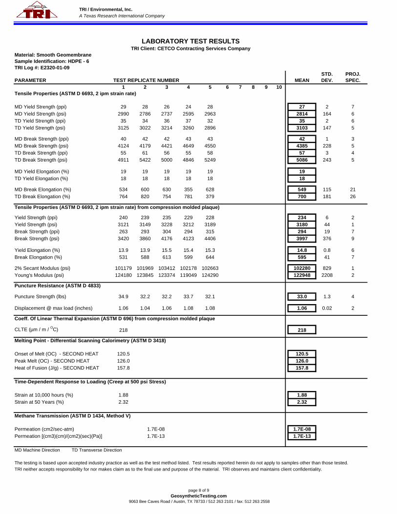
TRI / Environmental, Inc. A Texas Research International Company
LABORATORY TEST RESULTSTRI Client: CETCO Contracting Services Company
Material: Smooth GeomembraneSample Identification: HDPE - 6TRI Log #: E2320-01-09
STD. PROJ.PARAMETER TEST REPLICATE NUMBER MEAN DEV. SPEC.
1 2 3 4 5 6 7 8 9 10Tensile Properties (ASTM D 6693, 2 ipm strain rate)
MD Yield Strength (ppi) 29 28 26 24 28 27 2 7MD Yield Strength (psi) 2990 2786 2737 2595 2963 2814 164 6TD Yield Strength (ppi) 35 34 36 37 32 35 2 6TD Yield Strength (psi) 3125 3022 3214 3260 2896 3103 147 5
MD Break Strength (ppi) 40 42 42 43 43 42 1 3MD Break Strength (psi) 4124 4179 4421 4649 4550 4385 228 5TD Break Strength (ppi) 55 61 56 55 58 57 3 4TD Break Strength (psi) 4911 5422 5000 4846 5249 5086 243 5
MD Yield Elongation (%) 19 19 19 19 19 19TD Yield Elongation (%) 18 18 18 18 18 18
MD Break Elongation (%) 534 600 630 355 628 549 115 21TD Break Elongation (%) 764 820 754 781 379 700 181 26
Tensile Properties (ASTM D 6693, 2 ipm strain rate) from compression molded plaque)
Yield Strength (ppi) 240 239 235 229 228 234 6 2Yield Strength (psi) 3121 3149 3228 3212 3189 3180 44 1Break Strength (ppi) 263 293 304 294 315 294 19 7Break Strength (psi) 3420 3860 4176 4123 4406 3997 376 9
Yield Elongation (%) 13.9 13.9 15.5 15.4 15.3 14.8 0.8 6Break Elongation (%) 531 588 613 599 644 595 41 7
2% Secant Modulus (psi) 101179 101969 103412 102178 102663 102280 829 1Young's Modulus (psi) 124180 123845 123374 119049 124290 122948 2208 2
Puncture Resistance (ASTM D 4833)
Puncture Strength (lbs) 34.9 32.2 32.2 33.7 32.1 33.0 1.3 4
Displacement @ max load (inches) 1.06 1.04 1.06 1.08 1.08 1.06 0.02 2
Coeff. Of Linear Thermal Expansion (ASTM D 696) from compression molded plaque
CLTE (µm / m / OC) 218 218
Melting Point - Differential Scanning Calorimetry (ASTM D 3418)
Onset of Melt (OC) - SECOND HEAT 120.5 120.5Peak Melt (OC) - SECOND HEAT 126.0 126.0Heat of Fusion (J/g) - SECOND HEAT 157.8 157.8
Time-Dependent Response to Loading (Creep at 500 psi Stress)
Strain at 10,000 hours (%) 1.88 1.88Strain at 50 Years (%) 2.32 2.32
Methane Transmission (ASTM D 1434, Method V)
Permeation (cm2/sec-atm) 1.7E-08Permeation [(cm3)(cm)/(cm2)(sec)(Pa)] 1.7E-13
MD Machine Direction TD Transverse Direction
The testing is based upon accepted industry practice as well as the test method listed. Test results reported herein do not apply to samples other than those tested.TRI neither accepts responsibility for nor makes claim as to the final use and purpose of the material. TRI observes and maintains client confidentiality.
1.7E-081.7E-13
page 8 of 9GeosyntheticTesting.com
9063 Bee Caves Road / Austin, TX 78733 / 512 263 2101 / fax: 512 263 2558

TRI / Environmental, Inc. A Texas Research International Company
LABORATORY TEST RESULTSTRI Client: CETCO Contracting Services Company
Material: Smooth GeomembraneSample Identification: HDPE - 9TRI Log #: E2320-01-09
STD. PROJ.PARAMETER TEST REPLICATE NUMBER MEAN DEV. SPEC.
1 2 3 4 5 6 7 8 9 10Tensile Properties (ASTM D 6693, 2 ipm strain rate)
MD Yield Strength (ppi) 33 34 36 37 30 34 3 8MD Yield Strength (psi) 3188 3077 3303 3458 3468 3299 170 5TD Yield Strength (ppi) 47 46 48 51 49 48 2 4TD Yield Strength (psi) 3197 3228 3288 3377 3322 3283 72 2
MD Break Strength (ppi) 49 51 50 43 42 47 4 9MD Break Strength (psi) 4734 4615 4587 4019 4855 4562 322 7TD Break Strength (ppi) 77 69 68 73 65 70 5 7TD Break Strength (psi) 5238 4842 4658 4834 4407 4796 304 6
MD Yield Elongation (%) 16 16 16 16 16 16 0TD Yield Elongation (%) 18 20 18 18 18 18 1
MD Break Elongation (%) 684 658 668 601 606 643 37 6TD Break Elongation (%) 851 818 770 831 738 802 47 6
Tensile Properties (ASTM D 6693, 2 ipm strain rate) from compression molded plaque)
Yield Strength (ppi) 247 258 243 264 254 253 8 3Yield Strength (psi) 3514 3472 3462 3465 3475 3477 21 1Break Strength (ppi) 188 175 173 179 181 179 6 3Break Strength (psi) 2674 2355 2464 2349 2476 2464 132 5
Yield Elongation (%) 14.3 14.1 14.3 14.0 14.3 14.2 0.1 1Break Elongation (%) 393 307 377 227 376 336 69 21
2% Secant Modulus (psi) 114262 112735 111848 113692 111878 112883 1079 1Young's Modulus (psi) 135611 135846 132458 140357 131798 135214 3401 3
Puncture Resistance (ASTM D 4833)
Puncture Strength (lbs) 46.6 45.0 42.8 37.7 44.2 43.3 3.4 8
Displacement @ max load (inches) 1.14 1.14 1.12 1.14 1.14 1.14 0.01 1
Coeff. Of Linear Thermal Expansion (ASTM D 696)
CLTE (µm / m / OC) 210 210
Melting Point - Differential Scanning Calorimetry (ASTM D 3418)
Onset of Melt (OC) - SECOND HEAT 121.1 121.1Peak Melt (OC) - SECOND HEAT 127.1 127.1Heat of Fusion (J/g) - SECOND HEAT 159.3 159.3
Time-Dependent Response to Loading (Creep at 500 psi Stress)
Strain at 10,000 hours (%) 1.81 1.81Strain at 50 Years (%) 2.26 2.26
Methane Transmission (ASTM D 1434, Method V)
Permeation (cm2/sec-atm) 1.6E-08Permeation [(cm3)(cm)/(cm2)(sec)(Pa)] 1.6E-13
MD Machine Direction TD Transverse Direction
The testing is based upon accepted industry practice as well as the test method listed. Test results reported herein do not apply to samples other than those tested.TRI neither accepts responsibility for nor makes claim as to the final use and purpose of the material. TRI observes and maintains client confidentiality.
1.6E-131.6E-08
page 9 of 9GeosyntheticTesting.com
9063 Bee Caves Road / Austin, TX 78733 / 512 263 2101 / fax: 512 263 2558

Cetco500 psi Creep Test Results
LDPE Control
0.0
5.0
10.0
15.0
20.0
25.0
-4 -3 -2 -1 0 1 2 3 4 5 6 7
LOG TIME (HR)
%S
TR
AIN
TRI Log # E2280-19-05
Reference Temperature - 23C
10,000 hours 50 years
% Strain normalized at log time -2
12.00
18.48

Cetco500 psi Creep Test Results
LDPE 3
0.0
5.0
10.0
15.0
20.0
25.0
-4 -3 -2 -1 0 1 2 3 4 5 6 7
LOG TIME (HR)
%S
TR
AIN
TRI Log # E2280-19-05
Reference Temperature - 23C
10,000 hours 50 years
% Strain normalized at log time -2
9.48
14.76

Cetco500 psi Creep Test Results
LDPE 6
0.0
5.0
10.0
15.0
20.0
25.0
-4 -3 -2 -1 0 1 2 3 4 5 6 7
LOG TIME (HR)
%S
TR
AIN
TRI Log # E2280-19-05
Reference Temperature - 23C
10,000 hours 50 years
% Strain normalized at log time -2
8.50
13.25

Cetco500 psi Creep Test Results
LDPE 9
0.0
2.0
4.0
6.0
8.0
10.0
12.0
14.0
16.0
18.0
20.0
-4 -3 -2 -1 0 1 2 3 4 5 6 7
LOG TIME (HR)
%S
TR
AIN
TRI Log # E2280-19-05
Reference Temperature - 23C
10,000 hours 50 years
% Strain normalized at log time -2
7.21
11.09

Cetco500 psi Creep Test Results
HDPE Control
0.0
0.5
1.0
1.5
2.0
2.5
3.0
3.5
4.0
4.5
5.0
-4 -3 -2 -1 0 1 2 3 4 5 6 7
LOG TIME (HR)
%S
TR
AIN
TRI Log # E2280-19-05
Reference Temperature - 23C
10,000 hours 50 years
% Strain normalized at log time -2
2.83
3.42
Cetco500 psi Creep Test Results
HDPE 3
0.0
0.5
1.0
1.5
2.0
2.5
3.0
3.5
4.0
4.5
5.0
-4 -3 -2 -1 0 1 2 3 4 5 6 7
LOG TIME (HR)
%S
TR
AIN
TRI Log # E2280-19-05
Reference Temperature - 23C
10,000 hours 50 years
% Strain normalized at log time -2
2.50
2.99
Cetco500 psi Creep Test Results
HDPE 6
0.0
0.5
1.0
1.5
2.0
2.5
3.0
-4 -3 -2 -1 0 1 2 3 4 5 6 7
LOG TIME (HR)
%S
TR
AIN
TRI Log # E2280-19-05
Reference Temperature - 23C
10,000 hours 50 years
% Strain normalized at log time -2
1.88
2.32

Cetco500 psi Creep Test Results
HDPE 9
0.0
0.5
1.0
1.5
2.0
2.5
3.0
-4 -3 -2 -1 0 1 2 3 4 5 6 7
LOG TIME (HR)
%S
TR
AIN
TRI Log # E2280-19-05
Reference Temperature - 23C
10,000 hours 50 years
% Strain normalized at log time -2
1.81
2.26

125
VITA
Archibald Stewart Filshill
Archie was born in Philadelphia in 1965 and has dual citizenship from the United
States and Great Britain.
He received a Bachelor’s degree in Electrical Engineering Technology from Temple
University in 1998 and a Master’s degree in Civil Engineering from Drexel University
in 1996.
Archie Filshill is currently President of CETCO Contracting Services Company
located in Trevose, PA. He joined CETCO in 1995 as Regional Manager of the
Environmental Lining Group and became Managing Director of CETCO Europe from
1995 to 2000. From 2000 to 2005 Filshill was Manager/Member of InterGeo Services,
LLC a specialty subcontractor in Geosynthetic and Geotechnical Construction. He
rejoined CETCO in 2005 with the acquisition of InterGeo as Manager of CETCO’s
Contracting Services Company. CETCO’s contracting group is focused on Design
Build and Value Engineering of Geo-Environmental construction projects. He is a
board member of the Delaware Valley GeoInstitute.