long term property prediction of polyethylene nanocomposites
TRANSCRIPT

APPROVED: Nandika A. D’Souza, Major Professor Witold Brostow, Committee Member Thomas Scharf, Committee Member Cheng Yu, Committee Member Reza Mirshams, Committee Member Rick Reidy, Interim Chair of the Department of
Materials Science and Engineering Costas Tsatsoulis, Dean of the College of
Engineering Sandra L. Terrell, Dean of the Robert B. Toulouse
School of Graduate Studies
LONG TERM PROPERTY PREDICTION OF POLYETHYLENE NANOCOMPOSITES
Ali Al-Abed Shaito, B.E.
Dissertation Prepared for the Degree of
DOCTOR OF PHILOSOPHY
UNIVERSITY OF NORTH TEXAS
December 2008

Shaito, Ali Al-Abed, Long Term Property Prediction of Polyethylene
Nanocomposites. Doctor of Philosophy (Materials Science and Engineering), December
2008, 184 pp. , 21 tables, 62 illustrations, references.
The amorphous fraction of semicrystalline polymers has long been thought to be a
significant contributor to creep deformation. In polyethylene (PE) nanocomposites, the
semicrystalline nature of the maleated PE compatibilizer leads to a limited ability to
separate the role of the PE in the nanocomposite properties. This dissertation investigates
blown films of linear low-density polyethylene (LLDPE) and its nanocomposites with
montmorillonite- layered silicate (MLS). Addition of an amorphous ethylene propylene
copolymer grafted maleic anhydride (amEP) was utilized to enhance the interaction
between the PE and the MLS. The amorphous nature of the compatibilizer was used to
differentiate the effect of the different components of the nanocomposites; namely the
matrix, the filler, and the compatibilizer on the overall properties.
Tensile test results of the nanocomposites indicate that the addition of amEP and
MLS separately and together produces a synergistic effect on the mechanical properties
of the neat PE. Thermal transitions were analyzed using differential scanning calorimetry
(DSC) to determine if the observed improvement in mechanical properties is related to
changes in crystallinity. The effect of d ispersion of the MLS in the matrix was
investigated by using a combination of X-ray diffraction (XRD) and scanning electron
microscopy (SEM). Mechanical measurements were correlated to the dispersion of the
layered silicate particles in the matrix. The nonlinear time dependent creep of the material

was analyzed by examining creep and recovery of the films with a Burger model and the
Kohlrausch-Williams-Watts (KWW) relation.
The effect of stress on the nonlinear behavior of the nanocomposites was
investigated by analyzing creep-recovery at different stress levels. Stress-related creep
constants and shift factors were determined for the material by using the Schapery
nonlinear viscoelastic equation at room temperature.
The effect of temperature on the tensile and creep properties of the
nanocomposites was analyzed by examining tensile and creep-recovery behavior of the
films at temperatures in the range of 25 to -100 oC. Within the measured temperature
range, the materials showed a nonlinear temperature dependent response. The time-
temperature superposition principle was successfully used to predict the long term
behavior of LLDPE nanocomposites.

ii
Copyright 2008
by
Ali Al-Abed Shaito

iii
ACKNOWLEDGEMENTS
The printed pages of this dissertation hold far more than the culmination of years
of study. These pages also reflect the relationships with many generous and inspiring
people I have met since beginning my graduate work. I owe my gratitude to all those
people who have made this dissertation possible and because of whom my graduate
experience has been one that I will cherish forever.
To my advisor Nandika D’Souza, a gracious mentor who helped me during my
doctoral work. I would like to thank her for her generous time and commitment.
Throughout my doctoral work she encouraged me to develop independent thinking and
research skills. She continually stimulated my analytical thinking and greatly assisted me
with scientific writing.
To my committee members, Dr. Witold Brostow, Dr. Thomas Scharf, Dr. Cheng
Yu, and Dr. Reza Mirshams for their comments and suggestions.
I am also grateful to the following former or current staff at University of North
Texas for their various forms of support during my graduate study—Alberta Caswell,
Wendy Agnes, Joan Jolly , Olga Reyes, Lindsay Quinn for departmental assistance , John
Sawyer for insuring a safe work environment in the labs, and David Garrett for
microscopy training.
To my invaluable network of supportive and loving friends without whom I could
not have survived the process: Laxmi Sahu, Siddhi Pendse, Koffi Dagnon, Sunny

iv
Ogbomo, Shailesh Vidhate just to name few not to miss anyone. I wish all of you
good luck in your work.
Most importantly, none of this would have been possible without the love and
patience of my family. My immediate family, to whom this dissertation is dedicated to,
has been a constant source of love, concern, support and strength all these years. I would
like to express my heart- felt gratitude to my family.

v
TABLE OF CONTENTS
Page
ACKNOWLEDGEMENTS ............................................................................................... iii
LIST OF TABLES ..............................................................................................................ix
LIST OF FIGURES ............................................................................................................xi Chapters
1. INTRODUCTION .......................................................................................1
1.1 Objectives of Dissertation ................................................................2
1.2 Dissertation Outline .........................................................................3
2. POLYMER-CLAY NANOCOMPOSITES: STRUCTURE-PROPERTY RELATIONSHIP .........................................................................................6
2.1 Matrix: Polyethylene (PE) ...............................................................8
2.2 Filler: Clay .......................................................................................9
2.3 Compatibilizer: Thermoplastic Elastomer (TPE) ..........................13
2.4 Processing of Polymer Nanocomposites........................................14
2.5 Characterization of Polymer Nanocomposites...............................16
2.5.1 X-Ray Diffraction (XRD) ..................................................18
2.5.2 Transmission Electron Microscopy (TEM) and Spectroscopy ......................................................................19
2.5.3 Differential Scanning Calorimetry (DSC) .........................22
2.5.4 Dynamic Mechanical Thermal Analysis (DMTA) ............23
2.6 Modeling Long Term Properties in Polymers ...............................26
2.6.1 Mechanical Analogs for Viscoelastic Materials ................26
2.6.2 Findley Power Law ............................................................35
2.6.3 Kohlrausch -Williams-Watts (KWW) Relation .................35
2.6.4 Schapery Integral Representation ......................................36
2.7 References ......................................................................................39

vi
3. NONLINEAR CREEP DEFORMATION IN POLYETHYLENE NANOCOMPOSITES: EFFECT OF COMPOSITION OF ETHYLENE-
PROPYLENE COPOLYMER ON ROOM TEMPERATURE CREEP DEFORMATION ......................................................................................40
3.1 Introduction ....................................................................................40
3.2 Experimental ..................................................................................43
3.2.1 Materials.............................................................................43
3.2.2 Sample Preparation ............................................................43
3.2.3 X-Ray Diffraction (XRD) ..................................................44
3.2.4 Focused Ion Beam/Scanning Electron Microscopy (FIB/SEM) .........................................................................44
3.2.5 Differential Scanning Calorimetry (DSC) .........................45
3.2.6 Tensile Testing ...................................................................45
3.2.7 Creep Testing .....................................................................45
3.3 Results and Discussion ..................................................................46
3.3.1 Dispersion of MLS in the LLDPE Matrix .........................46
3.3.2 Crystallization Effects........................................................55
3.3.3 Tensile Stress-Strain Results..............................................58
3.3.4 Creep Response..................................................................61
3.4 Error Analysis ................................................................................75
3.5 Conclusions ....................................................................................78
3.6 References ......................................................................................79
4. EFFECT OF TEMPERATURE ON MOLECULAR RELAXATIONS IN
POLYETHYLENE NANOCOMPOSITES ...............................................81
4.1 Introduction ....................................................................................81
4.2 Experimental ..................................................................................84
4.2.1 Sample Preparation ............................................................84
4.2.2 Dynamic Mechanical Analysis (DMA) .............................84
4.2.3 Tensile Testing ...................................................................85
4.2.4 Creep Testing .....................................................................85
4.3 Results and Discussion ..................................................................85
4.3.1 DMA Results......................................................................85

vii
4.3.2 Tensile Test Results ...........................................................89
4.3.3 Creep Test Results .............................................................95
4.4 Conclusions ..................................................................................116
4.5 References ....................................................................................116
5. EFFECT OF STRESS ON ROOM TEMPERATURE MOLECULAR
RELAXATION ........................................................................................118
5.1 Introduction ..................................................................................118
5.2 Experimental ................................................................................119
5.2.1 Materials...........................................................................119
5.2.2 Sample Preparation ..........................................................120
5.2.3 Tensile Testing .................................................................120
5.2.4 Creep Testing ...................................................................121
5.3 Results and Discussion ................................................................121
5.3.1 Stress Dependence of Creep-Recovery Response ...........121
5.3.2 Burgers Modeling Parameters..........................................124
5.3.3 Modeling Parameter from KWW Function .....................127
5.4 Conclusion ...................................................................................130
5.5 References ....................................................................................131
6. SEPARATION OF STRUCTURAL TIME DEPENDENT
DEFORMATION DUE TO STRESS MAGNITUDE ............................132
6.1 Introduction ..................................................................................132
6.2 Experimental ................................................................................135
6.2.1 Sample Preparation ..........................................................135
6.2.2 Tensile Testing .................................................................136
6.2.3 Creep Testing ...................................................................136
6.3 Results and Discussion ................................................................137
6.3.1 Stress Effects on Creep ....................................................137
6.3.2 Schapery Modeling Parameters .......................................145
6.4 Conclusions ..................................................................................154
6.5 References ....................................................................................155

viii
7. SEPARATION OF STRUCTURAL TIME DEPENDENT DEFORMATION DUE TO TEMPERATURE .......................................157
7.1 Introduction ........................................................................................
7.2 Calculation of Temperature-Related Creep Variables .................159
7.2.1 Temperature Shift Factor .................................................160
7.3 Experimental ................................................................................161
7.3.1 Materials...........................................................................161
7.3.2 Sample Preparation ..........................................................161
7.3.3 Creep Testing ...................................................................162
7.4 Results and Discussion ................................................................162
7.4.1 Time/Temperature Equivalence .......................................162
7.4.2 Modeling Parameters of Schapery Model........................167
7.5 Conclusions ..................................................................................174
7.6 References ....................................................................................175
8. CONCLUSIONS......................................................................................176

ix
LIST OF TABLES
Page
2.1 Cloisite organoclays and their surfactants .............................................................12
2.2 Common ethylene-propylene copolymers used as elastomeric modifiers.............14
3.1 Summary of concentrations used ...........................................................................44
3.2 Values of 2θ and d for LLDPE/amEP/MLS nanocomposites ................................46
3.3 DSC results for LLDPE nanocomposites ..............................................................57
3.4 Tensile test results of LLDPE nanocomposites .....................................................59
3.5 Burgers fit parameters of LLDPE nanocomposites ...............................................68
3.6 KWW curve fitting parameters ..............................................................................74
4.1 Summary of concentrations used ...........................................................................84
4.2 DMA results showing variations in E’, E’’, and tan δ ...........................................88
4.3 Tensile test results of LLDPE nanocomposites at different temperatures .............94
4.4 Burgers modeling parameters of LLDPE nanocomposites at different temperatures .........................................................................................................105
4.5 KWW fit parameters of LLDPE nanocomposites at different temperatures .......112
5.1 Summary of concentrations used .........................................................................120
5.2 Burgers fit parameters of LLDPE nanocomposites .............................................125
5.3 KWW curve fitting parameters ............................................................................128
6.1 Summary of composition used.............................................................................136
6.2 Values of the nonlinear factors g0, g1, and aσ for LLDPE nanocomposites.........146
7.1 Summary of compositions used ...........................................................................162

x
7.2 Values of the nonlinear factors h0, h1, and aT for LLDPE nanocomposites at different temperatures ..........................................................................................168
7.3 Activation energy of LLDPE nanocomposites obtained from the mastercurves .173

xi
LIST OF FIGURES
Page
2.1 Schematic showing structural difference between LDPE and LLDPE ...................9
2.2 Montmorillonite clay..............................................................................................10
2.3 Edge view of montmorillonite structure of aluminum octahedron, which may also substitute elements of magnesium or iron, sandwiched between layers of silicon
tetrahedron .............................................................................................................11
2.4 Polymer-clay nanocomposite morphologies ..........................................................15
2.5 Schematic of X-ray diffraction ..............................................................................18
2.6 Photograph of a FIB workstation ...........................................................................21
2.7 University of North Texas name and logo "tattooed" into a silicon wafer ............21
2.8 Schematic of DSC instrument................................................................................22
2.9 Mastercurve construction from experimental time (frequency)-temperature data 25
2.10 Schematic of Maxwell model ................................................................................28
2.11 Schematic of Maxwell model response to a constant stress ..................................29
2.12 Schematic of Kelvin model....................................................................................30
2.13 Schematic of response of Kelvin model to a constant input stress (creep)............31
2.14 Schematic of Burgers model ..................................................................................32
3.1 XRD patterns of LLDPE and amEP/MLS nanocomposites: (a) MLS (001) reflections, (b) PE (110) reflections .......................................................................48
3.2 XRD patterns of amEP/MLS nanocomposites showing amEP amorphous halo...49
3.3 FIB/SEM images of (a) LLDPE/1% MLS nanocomposite, (b) LLDPE/1% amEP/1% MLS, (c) LLDPE/1% amEP/2% MLS, (d) LLDPE/2% amEP/1% MLS,
and (e) LLDPE/2% amEP/2% MLS nanocomposites ...........................................53
3.4 FIB/SEM images of (a) amEP /1% MLS nanocomposite, (b) amEP/ 3% MLS....54
xii
3.5 DSC thermograms: (a) second heating; (b) first cooling of LLDPE/amEP/MLS nanocomposites; (c) second heating and first cooling of amEP ............................57
3.6 Stress-strain curve of LLDPE nanocomposites at room temperature ....................59
3.7 Stress-strain curve of amEP/MLS nanocomposites at room temperature .............61
3.8 Creep-recovery curves of LLDPE/amEP/MLS nanocomposites at room .............62
3.9 Creep-recovery curves of amEP/MLS nanocomposites at room temperature .......63
3.10 Creep-recovery schematic......................................................................................64
3.11 Comparison of creep-recovery compliance of LLDPE and its nanocomposites at room temperature: (a) pure LLDPE, (b) LLDPE/1% MLS, (c) LLDPE/1% amEP,
and (d) LLDPE/1% amEP/1% MLS ......................................................................67
3.12 Comparison of experimental data to the Burgers model and the KWW function .68
3.13 Burgers retardation time comparison of LLDPE and amEP nanocomposites .......71
3.14 Retardation time comparison of LLDPE and amEP nanocomposites ...................73
3.15 Comparison of βkww for the different LLDPE and amEP nanocomposites............73
3.16 Error analysis showing overly of (a) tensile test; (b) creep test; (c) DSC test for pure LLDPE samples .............................................................................................77
4.1 DMA results showing (a) E’, (b) E”, and (c) tan δ versus temperature of LLDPE
nanocomposites ......................................................................................................87
4.2 Stress-strain curve of LLDPE nanocomposites at room temperature ....................90
4.3 Stress-strain curve of (a) pure LLDPE, (b) PE/1% MLS, (c) PE/1% amEP, (d) PE/1% amEP/1% MLS at different temperatures ..................................................93
4.4 Creep-recovery curves of LLDPE nanocomposites at room temperature .............95
4.5 Creep-recovery of LLDPE nanocomposites: (a) pure LLDPE, (b) PE/1% MLS, (c) PE/1% amEP, (d) PE/1% amEP/1% MLS at different temperatures .....................98
4.6 Creep-recovery analysis of LLDPE nanocomposites: (a) pure LLDPE, (b) PE/1% MLS, (c) PE/1% amEP, (d) PE/1% amEP/1% MLS at different temperatures ...101

xiii
4.7 Experimental and theoretical (Burgers and KWW ) results of LLDPE nanocomposites: (a) pure LLDPE, (b) PE/1% MLS, (c) PE/1% amEP, (d) PE/1%
amEP/1% MLS at different temperatures ............................................................104
4.8 Temperature dependence of Burgers EM .............................................................107
4.9 Temperature dependence of Burgers τ.................................................................109
4.10 Temperature dependence of retardation time values obtained from the KWW fit113
4.11 Temperature dependence of β values obtained from the KWW fit .....................114
5.1 Creep compliance versus time plot of LLDPE nanocomposites: (a) pure LLDPE, (b) PE/1% MLS, (c) PE/1% amEP, (d) PE/1% amEP/1% MLS at room
temperature...........................................................................................................123
5.2 Comparison of experimental data to the Burgers model and the KWW function for 50% yield stress..............................................................................................124
5.3 Burgers retardation time comparison of LLDPE nanocomposites ......................127
5.4 KWW retardation time comparison of LLDPE nanocomposites ........................129
5.5 Comparison of βkww for the different LLDPE nanocomposites ........................129
6.1 Creep compliance versus time plot of LLDPE nanocomposites: (a) pure LLDPE, (b) PE/1% MLS, (c) PE/1% amEP, (d) PE/1% amEP/1% MLS at room
temperature...........................................................................................................139
6.2 Mastercurve of linear transient compliance at 25 oC of (a) LLDPE, (b) PE/MLS 1,
(c) PE/amEP1, (d) PE/amEP1/MLS 1, (e) PE/amEP1/MLS 2, (f) PE/amEP2/MLS 1, and (g) PE/amEP2/MLS 2 ...............................................................................141
6.3 Creep compliance versus time plot of LLDPE nanocomposites: (a) amEP, (b)
amEP/1% MLS, (c) amEP/3% MLS at room temperature ..................................143
6.4 Mastercurve of linear transient compliance at 25 oC of amEP/MLS
nanocomposites ....................................................................................................144
6.5 Creep-recovery curves of LLDPE nanocomposites at room temperature ...........145
6.6 Experimental and theoretical (Schapery model) comparison of (a) creep
compliance and (b) recovery compliance ............................................................148
6.7 Stress dependence of the stress shift factor g0 .....................................................149

xiv
6.8 Stress dependence of the stress shift factor g1 .....................................................151
6.9 Stress dependence of the stress shift factor aσ .....................................................152
6.10 Stress dependence of the stress shift factor g2 .....................................................154
7.1 Creep-recovery of LLDPE nanocomposites (a) pure LLDPE (b) PE/1% MLS (c)
PE/1% amEP(d) PE/1% amEP/1% MLS at different temperatures.....................165
7.2 The temperature dependent creep compliance mastercurve ................................167
7.3 Variation of temperature dependent creep constant h0 with temperature ............170
7.4 Variation of temperature dependent creep constant h1 with temperature ............171
7.5 Variation of the temperature dependent shift factor h2 with temperature............172
7.6 Variation of the shift factor aT with temperature .................................................173
8.1 Schematic explaining material behavior during deformation ..............................184

1
CHAPTER 1
INTRODUCTION
When a polymer is used as a structural material, it is important that it be capable
of withstanding applied stresses and resultant strains over its service life. Polymers are
generally viscoelastic materials, having the properties of solids and viscous liquids. These
properties are time and temperature dependent. Poor creep resistance and dimensional
stability of polymers are generally a deficiency, limiting their service durability and
safety. This presents a barrier for their further expansion of their applications particularly
in automotive and aviation industries. Improving the creep resistance is a key factor in
ensuring their long term durability.
Creep is the time dependent strain (elongation) for materials under a constant
stress. For polymers, creep deformation is an important and powerful experimental
method to study many of their physical properties including viscoelastic behavior. For
viscoelastic materials such as polyethylene (PE), the load response is time dependent. At
very low stresses, the stress-strain relationship is time independent, and the material can
be approximated as a linear viscoelastic material. However, PE is in general a nonlinear
viscoelastic material and the constitutive relationship is dependent on stress/strain and
temperature. When the time-dependent material properties are independent of
stress/strain, a single compliance-time curve can define the creep behavior under different
stress levels. Such a material is categorized as linear viscoelastic. Otherwise, the material
2
properties are dependent on stress and a group of compliance time curves are needed to
describe the viscoelastic response of the material.
The creep properties of polymers can be enhanced by the addition of nanofillers.
Montmorillonite layered silicate (MLS) is used as a nanofiller because of its nanometer
scale dimension, which increases the interfacial interaction between MLS and the
polymer. The resulting structure in the polymer and MLS is called a polymer
nanocomposite. The advent of nanocomposites has led to increased interest in the creep
response of these materials. In particular, polyethylene is non polar and the limited
interaction with the surfactants on the clay is overcome by using a maleated
compatibilizer. The contributions and synergisms of a three component system on creep
are further complicated when two of the three components are crystallizable. Thus in this
work we focus on using a maleated polyethylene as a compatibilizer.
1.1 Objectives of Dissertation
The objective of this dissertation is to investigate the individual and synergistic
effects of adding montmorillonite layered silicate (MLS) and an amorphous ethylene
propylene copolymer grafted with maleic anhydride (amEP) into linear- low density
polyethylene (LLDPE) hence forth referred to as PE. The amorphous nature of the
compatibilizer helps in separating the role of the PE structure in the nanocomposite.
The effect of adding amEP and MLS on the overall properties of PE is obtained
by considering the following

3
1. Effect of amEP and MLS individually and separately on the room temperature tensile
and creep properties of PE nanocomposites.
2. Correlation of crystallinity and dispersion to the improvement in the mechanical
properties.
3. Effect of amEP and MLS on the stress and temperature response of PE
nanocomposites.
The structure-property relationship during creep is studied by considering constitutive
equations that describes the nonlinear viscoelastic behavior of the different materials
1. Burgers model and KWW function are used to correlate the morphological changes in
the nanocomposites to the retardation time and breadth of relaxation.
2. Schapery’s nonlinear equation is used to incorporate the structural changes in the
nanocomposites.
1.2 Dissertation Outline
Chapter 2 provides an overview of materials used in this study; their synthesis and
characterization and a comprehensive review of the physical models used to characterize
their viscoelastic behavior.
In Chapter 3, tensile and creep properties at room temperature, crystallinity, and
dispersion of the nanocomposites are studied and compared with the pure matrix.
Structure-property relationship in the materials was investigated by considering nonlinear
constitutive models and empirical equations that predicts the creep behavior in the
nanocomposites and relates it to the presence of MLS. Retardation time and breadth of
relaxation effects were examined by the Burgers and KWW models.

4
In Chapter 4, the effect of temperature on molecular relaxation was analyzed by
examining creep and recovery of the films at temperatures in the range of 25 and -100 oC.
The Burgers model was used to show the relationship between creep behavior and
retardation time. The individual creep compliance curves for each temperature were fitted
considering a polymeric system with a distribution of relaxation times; relevant
parameters such as the Kohlrausch-Williams-Watts (KWW) β relation were evaluated.
In Chapter 5, the effect of stress on the creep resistance of these materials was
investigated. Creep tests were conducted at different stress levels (10, 25, and 50% yield
stress). The nonlinear viscoelastic behavior of the material was modeled using Burgers
viscoelastic model and was seen to fit the creep data very well. It was also possible to
correlate the creep behavior to a polymeric system with a distribution of relaxation times
by considering KWW stretched exponential function.
In Chapter 6, effect of stress on the nanocomposites was investigated using
Schapery non- linear equation. The effects of adding MLS separately to the amEP was
investigated.
In Chapter 7, the relationship between deformation, time, and temperature of PE
nanocomposites was studied. For both chapters, the films were subjected to creep and
recovery in the tension mode and the time/stress/temperature related creep behavior was
studied. Smooth mastercurves are constructed using time-temperature-stress
superposition principles (TTSSP). The temperature-related creep constants and shift
factors were determined for the material using Schapery nonlinear viscoelastic equation.

5
The predicting results confirm the enhanced creep resistance of nanofillers even at
extended time scales and low temperatures.
Chapter 8 provides summary of results.
6
The addition of inorganic nanoparticles to polymeric systems resulted in the
introduction of a new set of materials known as polymer nanocomposites (PNs). These
materials exhibit multifunctional, high performance polymer characteristics beyond these
found in traditional filled polymeric systems. Multifunctional features include improved
thermal resistance and/or flame retardance, moisture resistance, improved mechanical
properties, decreased permeability, charge dissipation, and chemical resistance.
Polymer nanocomposites have emerged as a new area of research in the past few
years. The term “composite” is generally used to define a material that is made of more
than one component. Depending on the matrix, three types of composites exist:
polymeric, metallic, and ceramic composites. Composites consisting of components
where at least 1 dimension is < 10 nm are termed nanocomposites. Organically modified
layered silicates have been widely used in modern plastics as property enhancers. These
properties include improvement in mechanical, thermal, and flame retardance properties
.The enhancement in properties at low concentrations (2-6 wt %) has been reported by
many researchers. Hambir et al. [1] studied the effect of adding 4% octadecylamine
(ODA)-modified montmorillonite (MMT) clay to polypropylene (PP). They found that
the incorporation of the clay in a platelet form results in a significant improvement in the
thermal stability of PP. The temperature at the onset of degradation increases from about
CHAPTER 2
POLYMER –CLAY NANOCOMPOSITES: STRUCTURE-PROPERTY
RELATIONSHIP

7
270 to about 330 °C. The enhancement in the thermal stability of the PP/clay composites
can be attributed to the decreased permeability of oxygen due to the clay platelets in the
PP/clay composites. They also found that the PP/clay composite exhibits higher storage
modulus over the entire temperature range. The increase in the storage modulus is about
56%. Gilman et al. [2] found that polymer layered-silicate clay nanocomposites have the
unique combination of reduced flammability and improved physical properties. The
mechanical properties of a nylon-6 layered-silicate nanocomposite, with a silicate mass
fraction of only 5%, show excellent improvement over those for the pure nylon-6. The
nanocomposite exhibits a 40% higher tensile strength, 68% greater tensile modulus, 60%
higher flexural strength, and a 126% increased flexural modulus. The nylon-6
nanocomposite has a 63% lower HRR than the pure nylon-6. This suggests the improved
flammability properties of the nanocomposite as compared to the pure polymer matrix.
Dumont et al. [3] studied the barrier properties of PP/organoclay nanocomposites. They
found that improvements in the helium barrier properties are obtained with low
concentrations of the compatibilizer and filler (3 wt % each). They explained this effect
by changes in the arrangement of the clay platelets and by the state of the amorphous
domains.
This chapter presents an overview of polymer nanocomposites with a discussion
of a) the PE matrix used for preparation of the PE nanocomposites films, b) the type of
clay used in this study, c) common processing approaches to polymer nanocomposites, d)
characterization techniques relevant to this dissertation, and e) physical models used to
describe their viscoelastic behavior.
8
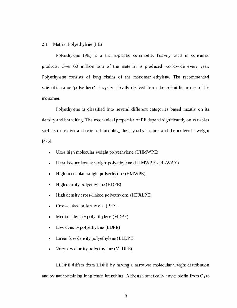
2.1 Matrix: Polyethylene (PE)
Polyethylene (PE) is a thermoplastic commodity heavily used in consumer
products. Over 60 million tons of the material is produced worldwide every year.
Polyethylene consists of long chains of the monomer ethylene. The recommended
scientific name 'polyethene' is systematically derived from the scientific name of the
monomer.
Polyethylene is classified into several different categories based mostly on its
density and branching. The mechanical properties of PE depend significantly on variables
such as the extent and type of branching, the crystal structure, and the molecular weight
[4-5].
Ultra high molecular weight polyethylene (UHMWPE)
Ultra low molecular weight polyethylene (ULMWPE - PE-WAX)
High molecular weight polyethylene (HMWPE)
High density polyethylene (HDPE)
High density cross- linked polyethylene (HDXLPE)
Cross-linked polyethylene (PEX)
Medium density polyethylene (MDPE)
Low density polyethylene (LDPE)
Linear low density polyethylene (LLDPE)
Very low density polyethylene (VLDPE)
LLDPE differs from LDPE by having a narrower molecular weight distribution
and by not containing long-chain branching. Although practically any α-olefin from C3 to
9
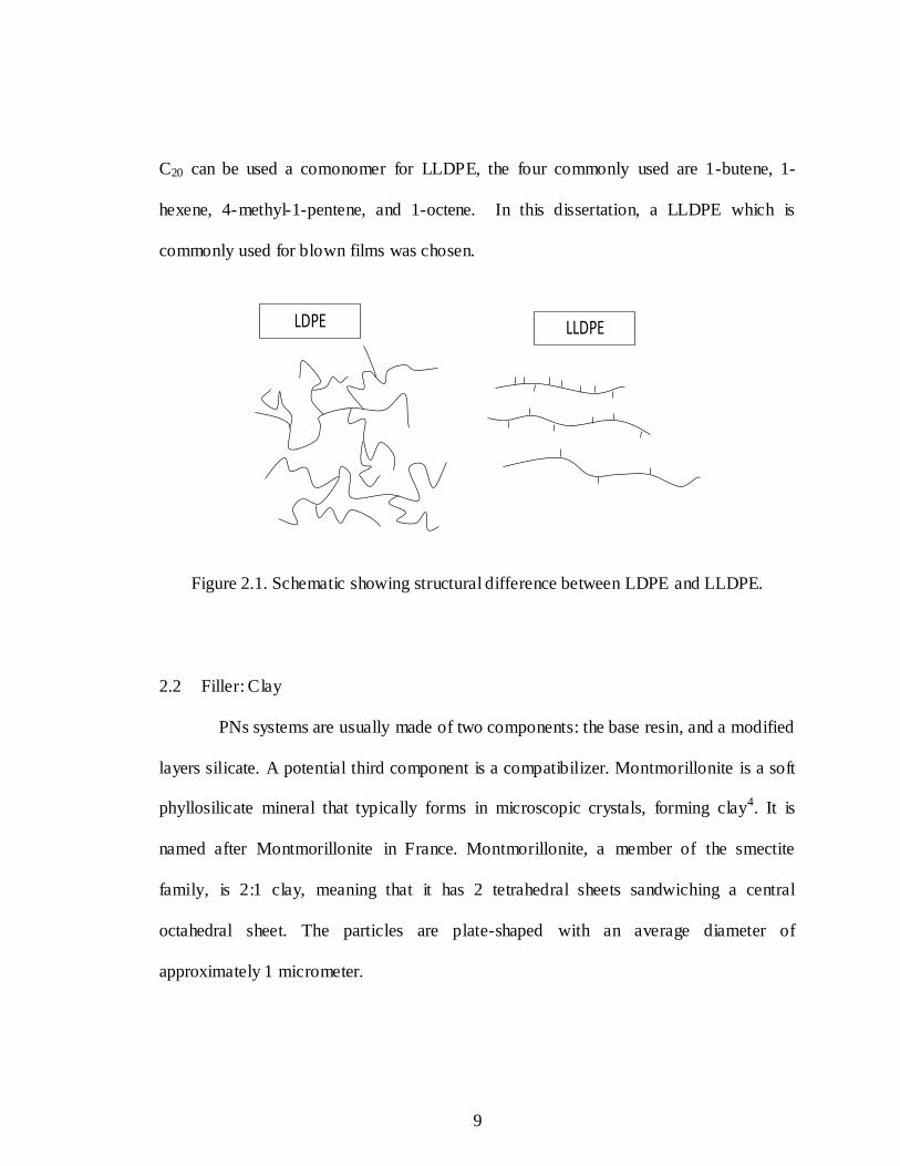
C20 can be used a comonomer for LLDPE, the four commonly used are 1-butene, 1-
hexene, 4-methyl-1-pentene, and 1-octene. In this dissertation, a LLDPE which is
commonly used for blown films was chosen.
LDPE LLDPE
Figure 2.1. Schematic showing structural difference between LDPE and LLDPE.
2.2 Filler: Clay
PNs systems are usually made of two components: the base resin, and a modified
layers silicate. A potential third component is a compatibilizer. Montmorillonite is a soft
phyllosilicate mineral that typically forms in microscopic crystals, forming clay4. It is
named after Montmorillonite in France. Montmorillonite, a member of the smectite
family, is 2:1 clay, meaning that it has 2 tetrahedral sheets sandwiching a central
octahedral sheet. The particles are plate-shaped with an average diameter of
approximately 1 micrometer.

10
Figure 2.2. Montmorillonite clay.
Silica is the dominant constituent of the montmorillonite clay, with alumina being
essential. The chemical structure of montmorillonite is shown in the figure. It is a sheet
structure consisting of layers containing the tetrahedral silicate layer the octahedral
alumina layer. The tetrahedral silicate layer consists of SiO4 groups linked together to
form a hexagonal network of the repeating units. The alumina layer consists of two sheets
of closely packed oxygens or hydroxyls, between which octahedrally coordinated
aluminum atoms are embedded in such a way that they are equidistant from six oxygens
or hydroxyls. The two tetrahedral layers sandwich the octahedral layer. The three layers
form one clay sheet that has a thickness of 0.96 nm. The chemical formula of
montmorillonite clay is Na1/3(Al5/3Mg1/3) Si4O10(OH)2 . In its natural state Na+ resides on
the MMT clay surfaces.

11
Figure 2.3. Edge view of montmorillonite structure of aluminum octahedron, which may also substitute elements of magnesium or iron, sandwiched between layers of silicon
tetrahedron.
Southern clay products (SCP) manufactures and markets cloisite additives. Their
montmorillonite organoclays are surface modified to allow dispersibility and miscibility
with many different resin systems for which they are designed to improve properties.
Cloisite MMT clays are Cloisite Na+, 15A, 20A, 30B, 93A, 25A, and 10A.
Cloisite Na+ is a natural montmorillonite. This additive improves various physical
properties such as reinforcement, heat deflection temperature (HDT), coefficient of linear
thermal expansion (CLTE), and barrier properties.
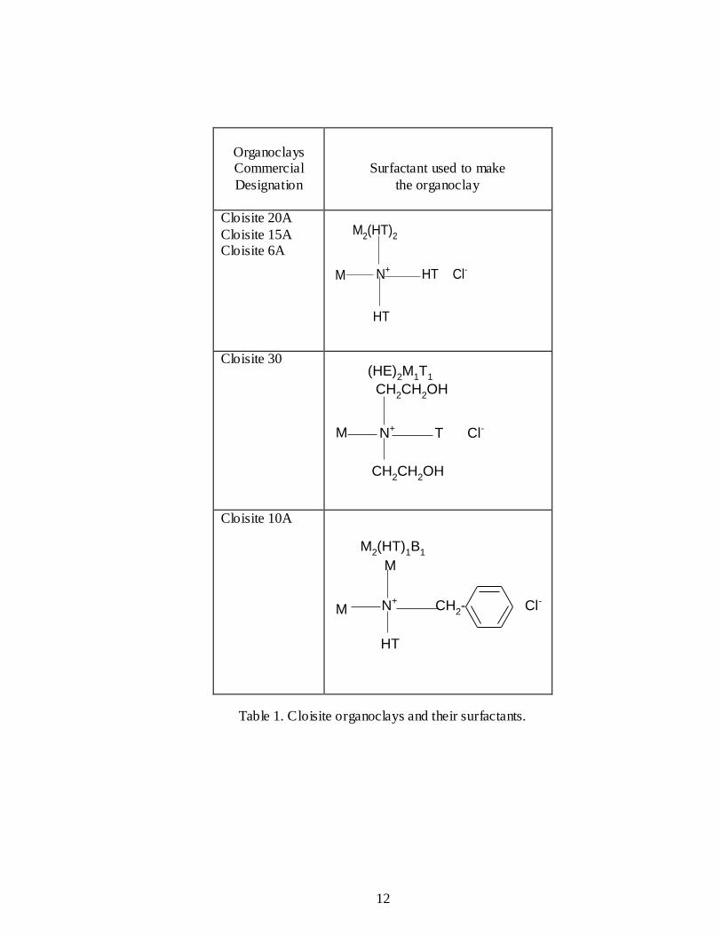
Cloisite 15A, 20A, 25A, and 30B are natural montmorillonite modified with a quaternary
ammonium salt.
Cloisite 93A is a natural montmorillonite modified with a ternary ammonium salt.
12
Organoclays Commercial
Designation
Surfactant used to make
the organoclay
Cloisite 20A
Cloisite 15A Cloisite 6A
N+ HT Cl-
M2(HT)
2
M
HT
Cloisite 30
CH2CH
2OH
CH2CH
2OH
N+ T Cl- M
(HE)2M
1T
1
Cloisite 10A
N+ CH2- Cl-
M
M2(HT)
1B
1
HT
M
Table 1. Cloisite organoclays and their surfactants.

13
2.3 Compatibilizer: Thermoplastic Elastomer (TPE)
Since nanocomposites require chemical interaction between the clay and the
matrix, non polar polymers like PE utilize a polar compatibilizer, typically thermoplastic
elastomers. Thermoplastic elastomers (TPE) or commonly known as thermoplastic
rubbers, are a class of copolymers which are usually a mixture of a plastic and a rubber.
They consist of materials having both thermoplastic as well as elastomeric properties.
Thermoplastic elastomers show both properties of a rubbery material and plastic material.
The principal difference between thermoset elastomers and thermoplastic
elastomers is the type of crosslinking bond in their structures. Crosslinking is one of the
critical structural factors which contribute to the high elastic properties. The crosslink in a
thermoset polymer is a covalent bond created during the vulcanization process, while the
crosslink in a thermoplastic elastomer polymer is a weaker dipole or hydrogen bond or
takes place in only in one of the phases of the material.
Some generic classes of TPEs are styrenic block copolymers, polyolefin blends,
elastomeric alloys, thermoplastic polyurethanes, thermoplastic copolyester and
thermoplastic polyamides. Ethylene/propylene (EP) copolymers grafted with maleic
anhydride are obtained from ExxonMobil Chemical, Exxelor 1803 and Exxelor 1801; the
former is nearly free of crystallinity while the later has a high level of ethylene
crystallinity. Exxelor 1803 was used in this study as a coupling agent between the
nonpolar LLDPE matrix and MLS. Okada et al. [6] prepared blends of nylon 6 with
Exxelor 1801 and 1803 by melt blending. The effect of nylon 6 content and the
crystallinity of the EP copolymer on morphological, thermal and mechanical properties of

14
these blends were studied. The EP copolymer with some ethylene crystallinity was shown
to have better mechanical properties than the amorphous EP copolymer which also had
an improvement in the mechanical properties as compared to the neat nylon matrix.
Polymer Characterization Source
Exxelor 1803
43 wt% ethylene, 53 wt%
propylene, 1.14 wt% MA,
amorphous, Tm = 127 oC
ExxonMobil Chemical
Exxelor 1801
43 wt% ethylene, 53 wt%
propylene, 1.21 wt% MA,
crystalline, Tm = 127 oC
ExxonMobil Chemical
Table 2.2. Common ethylene-propylene copolymers used as elastomeric modifier [6].
2.4 Processing of Polymer Nanocomposites
Solution intercalation, in-situ polymerization, and melt processing are considered
the most convenient methods to disperse layered silicates into polymer nanocomposites
in an intercalated or exfoliated state.
Two types of structures are obtained from the processing techniques, intercalated
nanocomposites, where the polymer chains are sandwiched between silicate layers, and
exfoliated nanocomposites where the separated, individual silicate layers are more or less
uniformly dispersed in the polymer matrix. This type of new materials exhibits enhanced

15
properties such as increased Young’s and storage modulus, increased thermal stability
and barrier properties, and good flame retardency at filler levels less than 2%.
Figure 2.4. Polymer-clay nanocomposite morphologies.
Layered silicates are exfoliated into single layers using a solvent in which the
polymer is soluble. The layered silicates, due to the weak forces that hold the layers
together can be easily dispersed in an adequate solvent. The polymer then absorbs onto
the delaminated sheets, and when the solvent evaporates, the sheets reassemble
sandwiching the polymer to form an ordered, multilayered structure.
Solution intercalation is a technique that has been widely used with water-soluble
polymers to produce intercalated nanocomposites based on polyvinyl alcohol (P VOH)
and polyethylene oxide (PEO). When polymeric aqueous solutions are added into
dispersions of fully delaminated sodium layered silicate, the strong interaction between
the water soluble macromolecules and the silicate layers often triggers the rearrangement
of the layers as it occurs for PEO. In the presence of PVOH, the silicate layers are
colloidly dispersed resulting in a colloidal distribution of the nanoparticles in PVOH.

16
Polymer intercalation using this technique can be also performed in organic solvents.
Polyethylene oxide has been successfully intercalated in sodium MMT by dispersion in
acetonitrile allowing stoichiometric incorporation of one or two polymer chains between
the silicate layers and increasing the intersheet spacing from 0.98 to 1.36 and 1.71 nm,
respectively.
In melt intercalation, the layered silicate is mixed with the solid polymer matrix in
the molten state. Under these conditions, and if the layer surfaces are sufficiently
compatible with the selected polymer, the polymer can be inserted into the interlayer
space and form either an intercalated or an exfoliated nanocomposite. No solvent is
required.
In the in-situ polymerization approach, the layered silicate is swollen within the
liquid monomer or monomer solution so that the polymer formation can occur between
the intercalated sheets. Polymerization can be initiated by different polymerization
methods such as heat or radiation, diffusion of a suitable imitator, or an organic initiator
or an organic initiator fixed through cationic exchange inside the interlayer before the
swelling step of the monomer.
2.5 Characterization of Polymer Nanocomposites
There are three steps involved in the development of nanocomposites: (1) material
preparation, (2) property characterization, (3) material performance. The material
preparation involves the processing of the nanoparticles with the polymer matrix into
polymer nanocomposite. The next challenge is the determination of the degree and level
of dispersion of the nanoparticles in the polymer matrix. Characterization involves:

17
structure analysis and property measurement. Structure analysis is carried out using a
variety of microscopic and spectroscopic techniques, while property characterization is
diverse and depends on the individual application.
Due to the high selectivity of the size and structure of nanostructured materials,
the physical properties of these materials can be diverse. An essential task to develop
capability in the preparation of nanomaterials is property characterization of an individual
nanostructure with a well defined atomic structure.
Characterizing the properties of an individual nanoparticle presents a challenge to
many existing testing and measurement techniques because of many constraints such as
the size (length and diameter) which makes their manipulation rather difficult and
specialized techniques are needed for identifying and analyzing individual
nanostructures. The commonly used characterization techniques for nanocomposites are
Wide angle X-ray diffraction (WAXD) and small angle X-ray scattering (SAXS):
used to study dispersion and crystallinity.
Transmission electron microscopy (TEM), scanning electron microscopy (SEM),
and spectroscopy: used to study dispersion.
Thermal gravimetric analysis (TGA): used to study thermal stability.
Differential scanning calorimetry (DSC): used to study thermal properties.
Dynamic mechanical thermal analysis (DMTA): used to study thermo-mechanical
properties.
Optical microscopy: used to study dispersion.

18
2.5.1 X-Ray Diffraction (XRD)
Wide angle X-ray diffraction is the most commonly used technique to study the
degree of nanodispersions of MMT organoclay in polymer nanocomposites. Wide angle
x-ray diffraction measures the distance between the ordered crystalline layers of the
organoclay.
By using Bragg’s law
sin2sin d (Equation 1)
Where d is the spacing between the atomic planes in the crystalline phase and λ is the x-
ray wavelength.
Figure 2.5. Schematic of X-ray diffraction.
The intensity of the diffracted X-ray is measured as a function of the diffraction
angle 2θ and the specimen’s orientation. This diffraction pattern is used to identify
specimen’s crystalline phases and to measure its structural properties. WAXD is a non-
destructive technique and does not require excessive sample preparation which explains
the wide usage of this technique in materials characterization. Spacing changes (increase
19
or decrease) can be used to determine the type of polymer nanocomposite formed such
as:
Immiscible: no d-spacing change.
Decomposed/deintercalted: d-spacing decrease.
Intercalated: d-spacing increase.
Exfoliated: d-spacing outside the wide angle x-ray diffraction or so expanded or
disordered to give a signal.
2.5.2 Transmission Electron Microscopy (TEM) and Spectroscopy
One of the characteristics of polymer nanostructured materials is their small
particle size of the added particles. Direct imaging of these nanometer range particles is
only possible through transmission electron microscopy and scanning probe microscopy.
The uniqueness of TEM lies in the fact that it can provide a real space image of the atoms
in the nanocrystals. Today’s TEM provides not only atomic resolution images, but also
chemical information at a spatial resolution of 1 nm or better allowing the identification
of the chemistry of a single nanocrystal.
TEM sample preparation is of importance for obtaining a TEM image with good
resolution. The basic requirement is that the specimen should be thin enough to be
transparent to the electron beam. There are several methods for TEM specimen
preparation:
Ion-milling: for almost all kind of materials.
Electropolishing: for conductive bulk materials.

20
Microtoming: for polymeric and biological samples.
Crushing powders: the simplest way to prepare TEM specimens, but
microstructural details can be lost.
Transmission electron microscopy allows the observation of the overall
organoclay dispersion in the polymer nanocomposite sample. Clay dispers ion and
structure observed using TEM can determine the nature of clay nanocomposites as:
Immiscible
Intercalated
Exfoliated
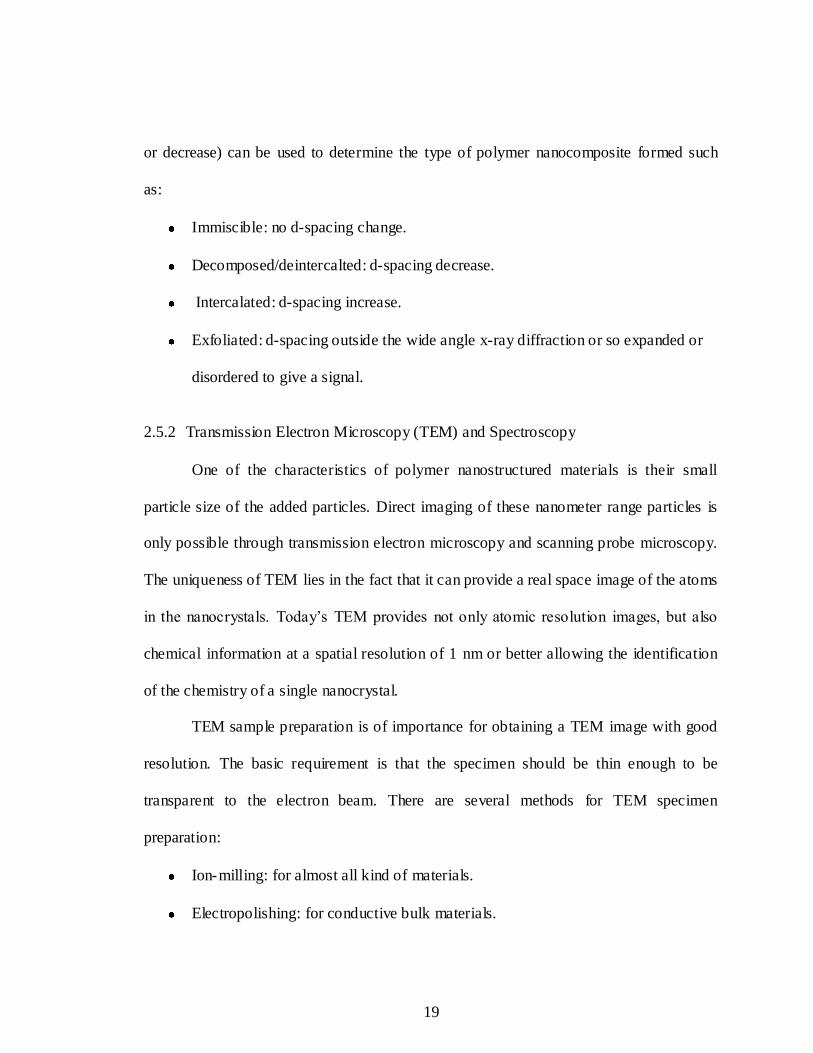
2.5.2.1 Focused Ion Beam (FIB)
Focused ion beam, also known as FIB, is a technique used particularly in the
semiconductor and materials science fields for site-specific analysis, deposition, and
ablation of materials.
The FIB is a scientific instrument that resembles a scanning electron microscope.
However, while the SEM uses a focused beam of electrons to image the sample in the
chamber, a FIB instead uses a focused beam of gallium ions. Gallium is chosen because it
is easy to build a gallium liquid metal ion source (LMIS).
21
Figure 2.6. Photograph of a FIB workstation.
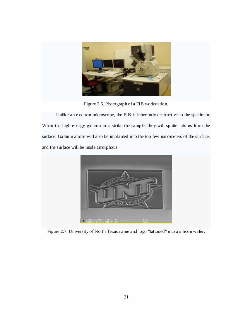
Unlike an electron microscope, the FIB is inherently destructive to the specimen.
When the high-energy gallium ions strike the sample, they will sputter atoms from the
surface. Gallium atoms will also be implanted into the top few nanometers of the surface,
and the surface will be made amorphous.
Figure 2.7. University of North Texas name and logo "tattooed" into a silicon wafer.

22
2.5.3 Differential Scanning Calorimetry (DSC)
Differential scanning calorimetry or DSC is a thermo-analytical technique in
which the difference in the amount of heat required to increase the temperature of a
sample and reference are measured as a function of temperature.
Figure 2.8. Schematic of DSC instrument [7].
In a DSC experiment, both the sample and reference are maintained at nearly the
same temperature. The basic principle that this technique involves is that when the
sample undergoes a physical transformation such as phase transitions, more (or less) heat
will need to flow to it than the reference to maintain both at the same temperature. By
observing the difference in heat flow between the sample and reference, differential
scanning calorimeters are able to measure the amount of heat absorbed or released during
such transitions.

23
2.5.4 Dynamic Mechanical Thermal Analysis (DMTA)
Dynamic mechanical properties refer to the response of the material as it is
subjected to a periodic force. These properties may be presented in terms of a dynamic
storage modulus, a dynamic loss modulus, and a mechanical damping factor.
For an applied stress varying sinusoidally with time, a viscoelastic material will
also respond with a sinusoidal strain. The sinusoidal variation in time is usually described
as a rate specified by the frequency ƒ = 2 Πω (f = Hz; ω = rad/sec). The strain of a
viscoelastic material is out of phase with the applied stress, by a phase angle, δ. This
phase lag is due to the time necessary for molecular motions and relaxations to occur. For
an elastic material, the phase angle is equal to zero, whereas for a viscous material the
phase angle is equal to 90o.
Dynamic stress ζ and strain ε can be represented by:
)sin(0 t (Equation 2)
)sin(0 t (Equation 3)
where ω is the angular frequency.
Dividing the stress by the strain to yield a modulus and using E′ and E′′ for the in phase
and the out-of -phase moduli respectively
''')sin(cos* iEEiEo
o (Equation 4)
Equation 4 shows that the complex modulus obtained by a dynamic mechanical
test consists of a “real” part and an “imaginary” part. The real (storage) part E′ describes
the ability of the material to store potential energy and release it upon deformation. The

24
imaginary (loss) part is associated with energy dissipation in the form of heat upon
deformation.
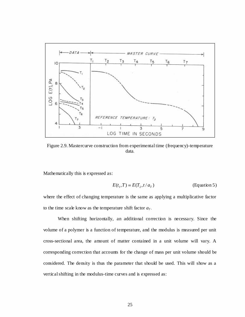
2.5.4.1 Time-Temperature Superposition (TTS)
The time-temperature correspondence states that there are two methods to
determine the polymer’s behavior at longer times. First, one may directly measure the
response at longer times. This technique is time consuming as the change is slow.
Secondly, one may carry out the relaxation experiment at a temperature T1 at
experimentally accessible time scales. The temperature is then increased to a temperature
T2. The curves at temperature T2 can be shifted horizontally to the right to give an exact
superposition of the curves measured at temperatures T1 and T2 in the areas where the
modulus values overlap. Thus, one can measure the complete modulus-time behavior by
applying the time-temperature correspondence principle to experimental measurements of
polymer relaxations carried out on experimental accessib le time scales.
25
Figure 2.9. Mastercurve construction from experimental time (frequency)-temperature data.
Mathematically this is expressed as:
)/,(),( 21 TatTETtE (Equation 5)
where the effect of changing temperature is the same as applying a multiplicative factor
to the time scale know as the temperature shift factor aT .
When shifting horizontally, an additional correction is necessary. Since the
volume of a polymer is a function of temperature, and the modulus is measured per unit
cross-sectional area, the amount of matter contained in a unit volume will vary. A
corresponding correction that accounts for the change of mass per unit volume should be
considered. The density is thus the parameter that should be used. This will show as a
vertical shifting in the modulus-time curves and is expressed as:
26
22
2
11
1
)(
)/,(
)(
),(
TT
atTE
TT
TtE T (Equation 6)
Division by temperature accounts for changes in modulus due to the dependence of
modulus on temperature and division by density accounts for the change per unit volume
with temperature.
2.6 Modeling Long Term Properties in Polymers
Viscoelastic materials have a specific set of characteristics that differentiate them
from elastic materials. Elastic materials store 100% of energy due to deformation when
compared to viscoelastic materials that do not store 100% of the energy under
deformation and lose or dissipate some of this energy. The ability to dissipate energy is
one of the main reasons for using viscoelastic materials for any application to cushion
shock, such as the materials used in running shoes or packing materials. The two other
main characteristics associated with viscoelastic materials are stress relaxation and creep.
Stress relaxation refers to the behavior of stress reaching a peak and then
decreasing or relaxing over time under a fixed level of strain. Creep is in some sense the
inverse of stress relaxation, and refers to the ability of viscoelastic materials to undergo
increased deformation under a constant stress, until an asymptotic level of strain is
reached.
2.6.1 Mechanical Analogs for Viscoelastic Materials
The classic way to derive viscoelastic constitutive models is through the use of
mechanical analogs [8]. These are simple mechanical models for fluid and solid
27
representations that are put together to produce viscoelastic effects. The simplest
mechanical analog for a linear elastic material is a spring. The simple constitutive
relationship for a spring relates the force (stress when force is divided by area) to the
elongation or displacement (strain when displacement is normalized by length of the
spring).
E (Equation 7)
Where ζ is the applied stress, E is the elastic modulus, and ε represents the resultant
strain. The mechanical analog for a Newtonian fluid is a dashpot. The simple constitutive
relationship for a dashpot indicates that the force in the fluid depends on the rate the
dashpot is displaced, or equivalently the velocity of the dashpot. The constitutive
parameter that relates force (stress) to displacement rate (strain rate) is viscosity η.
dt
d (Equation 8)
By making various combinations of spring and dashpot models, we can simulate the
behavior of a viscoelastic material, including stress relaxation and creep.
2.6.1.1 Maxwell Model
The simplest combination of the spring and dashpot is to put the spring in series
with the dashpot. This combination is known as the Maxwell model. This model
represents a fluid since it relaxes completely to zero stress and undergoes creep
indefinitely.
21 (Equation 9)

28
Where ε1 and ε2 are the strains of the spring and dashpot, respectively.
Since the stresses in both the spring and dashpot are the same, the strains in the spring in
the dashpot can be represented as
E1 ; 2 (Equation 10)
Figure 2.10.Schematic of Maxwell model.
Equations (9), (10) when combined give:
//..
E (Equation 11)
For a constant applied stress ζ
0.
(Equation 12)
Equation (11) allows the evaluation of the response to a step stress (creep) or step strain
(stress relaxation). To solve the differential equation in Equation (11), Laplace transform
is used. The Laplace transform of Equation (11) gives

29
)(1
)]0()([1
)0()( sssE
ss (Equation 13)
The response to a stress input ζ(t) is given by
)1
()( 0
t
Et (Equation 14)
Where E=ζ0/ε0. The creep compliance function is given by
t
E
ttD
1)()(
0
(Equation 15)
The response to the stress input of the Maxwell model is schematically represented in
Figure 2.
Figure 2.11. Schematic of Maxwell model response to a constant stress.
The Maxwell analog therefore reflects the instantaneous elastic deformation via
the spring, but the linear time response is inadequate in reflecting the non-Newtonian
viscous response of polymer systems. This is because, in creep, the dashpot undergoes
continuous deformation and the strain is time dependent. The recovery response of the
Maxwell analog is also inadequate. When the applied load is removed, the spring recoils
ζ
t
ζ0
ε
t
εo

30
elastically while the dashpot remains deformed. The extent of this deformation depends
on the viscous portion and the deformation is an irreversible process.
2.6.1.2 Kelvin-Voigt Model
In Kelvin model the spring and dashpot are connected in parallel. Based on the
geometry of the model, the dashpot will constrain the spring to have the same
deformation. The total stress is the sum of the stress in the spring and dashpot.
21 (Equation 16)
Which gives
.
E (Equation 17)
The above equation illustrates an important characteristic o f viscoelastic materials,
namely that the stress in the material depends not only on the strain, but also on the strain
rate.
Figure 2.12. Schematic of Kelvin model.

31
The Laplace transform of this equation for a step stress input gives
)]0()([)(0 sssEs
(Equation 18)
The corresponding strain can be written as
)()( 0
sEss (Equation 19)
The inverse Laplace transform of Equation (14) gives the strain response of the Kelvin-
Voigt element as
)]/exp(1[)( 0 tE
t (Equation 20)
The response is shown schematically in Figure 4.
Figure 2.13. Schematic of response of Kelvin model to a constant input stress (creep).
When the load is removed in the Kelvin model, the spring tries to recoil
elastically and this causes both spring and dashpot to reach their initial positions.
ζ
t
ζo
ε
t

32
However, this process is delayed due to the presence of dashpot (viscous component).
Real polymers behave viscoelastically. There is instant recoil of the elastic portion,
delayed reformation of both the elastic and viscous parts, and a permanent deformation of
the viscous part. Individual Maxwell and Kelvin models fail to explain the complex
viscoelastic behavior of polymer systems.
2.6.1.3 Burgers Model
Burgers model is a four-element model that is a combination of Maxwell and
Kelvin-Voigt models in series. The total strain is the sum of the elastic and viscous
strains represented by Maxwell element and the viscoelastic strain represented by Kelvin-
Voigt element.
321 (Equation 21)
Figure 2.14. Schematic of Burgers model.

33
1
01
E;
1
02
.
; 2
03
2
23
. E (Equation 22)
Substituting the values of ε1, ε2,, and ε3 into Equation(15) , one obtains
..
2
21.
1
..
21
21.
21
1
2
2 11
EEEEEE (Equation 23)
The response to a step stress input is given by
)exp(111
)(2211
0
t
E
t
Et (Equation 24)
Where η2=η2/E2 is the relaxation time.
When a stress ζ is applied, the Maxwell spring initially deforms. The Kelvin
spring and dashpot show a delayed deformation at longer times. When the applied force
is removed (recovery step), the Maxwell spring recovers completely. The Kelvin spring
and dashpot show delayed reformation. The Burgers model resembles the behavior of a
viscoelastic material and is thus used in our analysis.
2.6.1.4 Generalized Viscoelastic Constitutive Model
The strain behavior over time of a viscoelastic material is a function of the creep
function and the stress. Boltzmann (1844-1906) first generalized these observations by
saying that for a simple bar subject to a stress (t),the increment in stress over a small
time interval d would be:

34
dd
dd (Equation 25)
This assumes that the stress is continuous and differentiable in time. Given that the stress
is related to the strain via the creep function, Boltzmann postulated that an increment of
strain d , which depends on the complete stress history up to time t, would be related to
the increment of stress d at the specific time increment from to t through the creep
function D at the time t - as:
dd
dtDtd )()( (Equation 26)
The complete strain at a time t would then be obtained by integrating the strain
increments from time 0 to time t, over all the increments d :

35
t
dd
dtDt
0
)()()( (Equation 27)
2.6.2 Findley Power Law
Considering the creep curves of many polymers are similar to those of some
metals, many authors proposed several empirical mathematical models to represent the
creep data of polymers. Among then Findley, used the following empirical power
equation which could describe the creep behavior of many polymers with good accuracy
over a wide time scale
n
FFF t10 (Equation 28)
where the subscript F indicates the parameters associated with the Findley power law; n
is a constant independent of stress and generally less than one.; εF0 is the time
independent strain; and εF1 is the time dependent strain. εF0 and εF1 are functions of stress
and temperature.
The power law has been widely used to express stress-strain relationship for viscoelastic
materials.
2.6.3 Kohlrausch -Williams-Watts (KWW) Relation
The initial (for small strains) stress-strain behavior of polymers can be described
by the classical viscoelasticity theory. In the linear viscoelastic region, the strain, ε,
evolution with time can be obtained from Boltzmann superposition principle. For the case
of creep, the total strain may be expressed by
36
t
dtDt )()(
(Equation 29)
For systems with single retardation time η, the creep compliance, D, is given by
)]/exp(1[)( 0 tDtD
(Equation 30)
where D0 is the initial creep compliance.
Real systems are characterized by a distribution of characteristic times. A simple
empirical equation based on the KWW stretched function can be used to express the
exponential growth of the creep compliance, and the creep compliance is given by
])/exp(1[)( 0c
ctDtD
(Equation 31)
where βc takes values between 0 and 1. It quantifies the degree of retardation time
distribution; the KWW function implies a spectrum of retardation times whose breadth is
related to βc. τc is the mean retardation time of the retardation spectrum.
2.6.4 Schapery Integral Representation
In general, creep compliance is defined as the time dependent strain per unit stress
during a creep experiment. It is expressed as
)()(
ttD
(Equation 32)
The nonlinear viscoelastic constitutive equation derived by Schapery [9-11] has the
advantage of having a single time- integral form, even in the nonlinear region. The stress-
strain relation of this model is expressed as
37
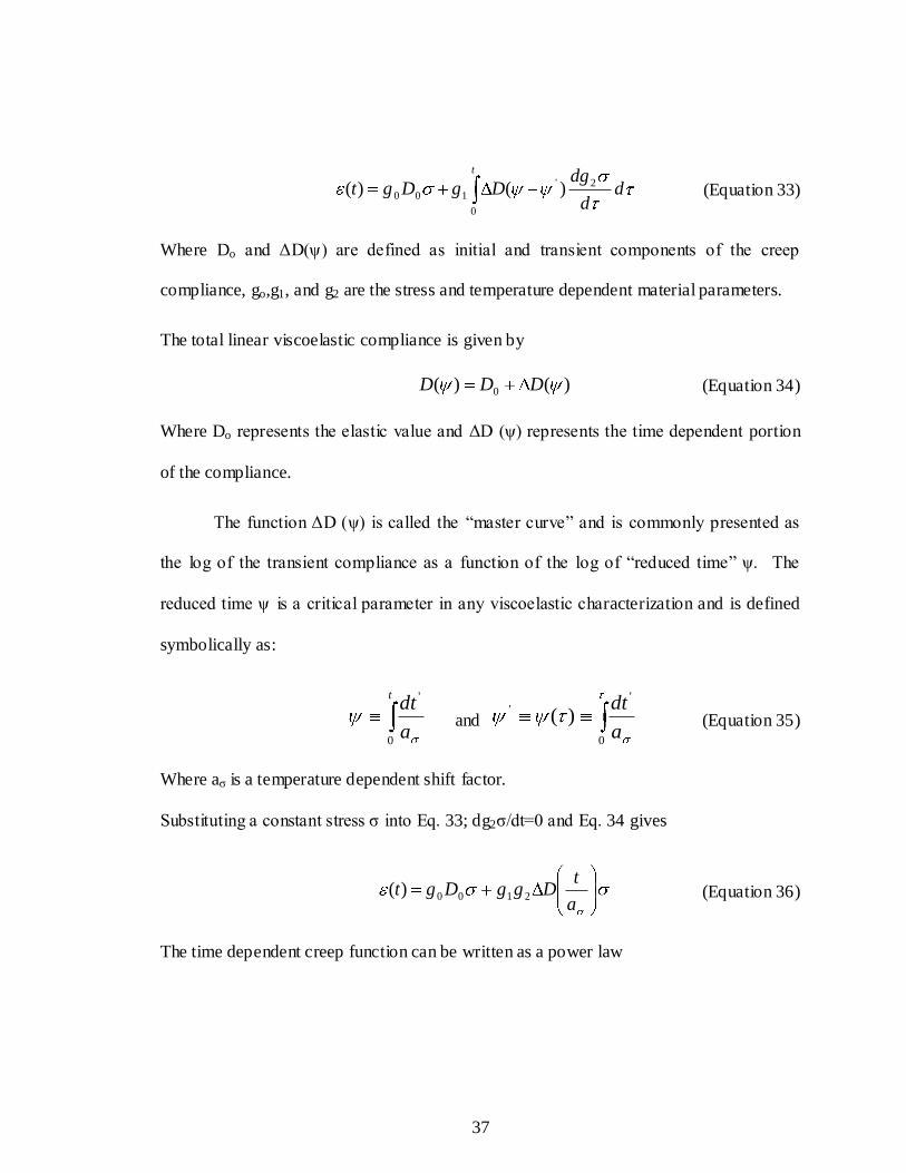
t
dd
dgDgDgt
0
2'
100 )()( (Equation 33)
Where Do and ΔD(ψ) are defined as initial and transient components of the creep
compliance, go,g1, and g2 are the stress and temperature dependent material parameters.
The total linear viscoelastic compliance is given by
)()( 0 DDD (Equation 34)
Where Do represents the elastic value and ΔD (ψ) represents the time dependent portion
of the compliance.
The function ΔD (ψ) is called the “master curve” and is commonly presented as
the log of the transient compliance as a function of the log of “reduced time” ψ. The
reduced time ψ is a critical parameter in any viscoelastic characterization and is defined
symbolically as:
t
a
dt
0
'
and 0
'' )(
a
dt (Equation 35)
Where aζ is a temperature dependent shift factor.
Substituting a constant stress ζ into Eq. 33; dg2ζ/dt=0 and Eq. 34 gives
a
tDggDgt 2100)( (Equation 36)
The time dependent creep function can be written as a power law

38
nCD 1)( (Equation 37)
This gives
n
nc ta
ggCDgt 211
00)( (Equation 38)
Equation 38 has a number of unknown parameters, so that additional information
is needed to obtain all parameters. The initial condition is at small strain levels where
Schapery equation becomes identical to the known linear viscoelastic creep equation
(go=g1=g2=aζ=1).
Schapery derived another expression for the recovery strain [10]
])()1[()(1
nnar aa
gt (Equation 39)
Where Δεa is the strain before unloading at ta and λ is the reduced time (t-ta)/ta.
Creep and recovery strains in Eqs 38 and 39 can be rewritten as
n
c tt 10)( (Equation 40)
])()1[()( nn
r aaAt (Equation 41)
Where ε0=g0D0ζ (the instantaneous strain after unloading), na
ggC 2111 (the
transient strain), and 1/ gA a ( a is the net strain at time just before unloading).

39
2.7. References
1. S Hambir, N Bulakh, P Kodgire, R Kalgaonkar, J Jog, Journal. of Polym. Sci.: Part B:
Polym. Phy. ,39, 446–450 (2001)
2. J. Gilman , Appl. Clay Sci., 15, 31–49 (1999)
3. MJ Dumont, A Reyna-Valencia, JP Emond, M Bousmina, Journal of Appl. Polym. Sci.
,103, 618–625 (2006)
4. A Guide to IUPAC Nomenclature of Organic Compounds, Blackwell Scientific
Publications, Oxford (1993)
5. J Kahovec, RB Fox, K Hatada, Pure and Applied Chemistry, 74, 1921–1956 (2002)
6. O. Okada, H. Keskkula, D.R. Paul “, Polymer, 42, 8715-8725 (2001)
7 . http:// pslc.ws/mactest/dsc.htm 8. J.J. Aklonis and W.J. MacKnight. Introduction to Polymer Viscoelasticity, John Wiley
& Sons: New York (1983).
9. R Schapery, Journal of Solids and Structures,2, 407-425 (1966)
10. R Schapery, Polymer Engineering and Science, 9,295-310 (1969)
11. R Schapery, International Journal of Solids and Structure,37,359-366 (2000)

40
CHAPTER 3
NONLINEAR CREEP DEFORMATION IN POLYETHYLENE NANOCOMPOSITES: EFFECT OF COMPOSITION OF ETHYLENE-PROPYLENE COPOLYMER ON
ROOM TEMPERATURE CREEP DEFORMATION
3.1. Introduction
Polymer nanocomposites are a class of materials composed of a polymeric matrix
in which fillers with nanoscale dimensions are embedded. The fillers improve the
physical and mechanical macroscopic properties of the nanocomposites dramatically.
Polymer nanocomposites show increased modulus, higher heat distortion temperature,
better barrier properties, and decreased thermal expansion coefficient [1, 2]. These
properties make them the material of choice in different applications such as the
construction of stratospheric balloons. However, because the application of polymer
nanocomposites can be limited by their poor dimensional stability, knowledge of the
creep resistance of polymer nanocomposites over a long period of time is of great
interest. The importance of creep resistance in polymers is underscored both in thick
sample geometries in automotive applications and in thin films (0.01 mm) for use in
scientific balloon applications. Balloons experience harsh stratospheric conditions that
require a material with good ductility. Balloons are made of thin polymeric films (10- to
20- m thickness) [3,4] with a number of properties, including low permeability, high
toughness, and structural stability.
The mechanical properties of polyethylene (PE) nanocomposites have been
studied by many researchers [5-7]. Liang et al. [6] studied the mechanical properties of

41
PE- montmorillonite layered silicate (MLS) nanocomposites compatibilized with
maleated polyethylene and found that increasing the content of maleated PE with a
silicate modified by a cationic surfactant could enhance the extent of intercalation. A
maximum increase in mechanical properties was achieved when a combination of 6 wt%
maleated PE and 3 wt % MLS was used. Wang et al. [8] investigated exfoliation and
intercalation in maleated PE/clay nanocomposites prepared by melt compounding. In
their investigation, the nanocomposites were completely exfoliated, and the mechanical
properties were dramatically improved when the PE had a higher grafting level of MA
than the critical level of 0.1%. A clay weight fraction of 5 wt % was used. Quintanilla et
al. [9] studied the effect of maleated polypropylene (PP) content on the mechanical
properties of PP nanocomposites. They found that clay dispersion and interfacial
adhesion are strongly affected by maleated PP content. The increase in content of polar
groups gave better interfacial adhesion and improved mechanical properties.
Creep resistance in nanocomposites can be ascribed to clay dispersion as well as
matrix properties. Thus, variations in clay content, compatibilization by maleated PE, and
the degree of dispersion are all parameters that affect creep [10-17]. Pegoretti et al. [11]
studied the creep deformation of polyethylene terephthlate (PET) filled with 1, 3, and 5
wt % layered silicate. An increase of 30% in modulus was obtained at a clay loading of 5
wt%. The creep compliance decreased slightly with the addition of clay. This decrease
suggests the beneficial effect of clay on the dimensional stability of the nanocomposite.
Yang et al. [14] studied the tensile creep resistance of polyamide 66 nanocomposites with
different filler shapes. The volume content of the nanoparticles was set to 1%. The creep

42
resistance of the nanocomposites was significantly enhanced by the nanoparticles without
sacrificing the tensile properties. The improvement was attributed to the good dispersion
of the surface-modified particles.
Previous work by our laboratory [18] studied the creep and tensile properties of
semicrystalline LLDPE/maleated PE/MLS nanocomposite to determine the effect of
semicrystalline maleated PE/MLS on room temperature creep. We showed synergistic
increase in tensile strength and modulus. The highest increase in strength (35%) was
obtained for the addition of 1% of both MLS and maleated PE. The results were
attributed to the addition of maleated PE, which acted as a coupling agent between PE
and MLS. The miscibility between PE and MLS was increased because of MA’s polar
nature. Non- linearity in creep behavior was analyzed by using the Burgers model.
Diffraction analysis and optical microscopy showed more uniform dispersion in the
maleated nanocomposite. Maleated nanocomposites showed lower retardation time. Since
the maleated PE contributed to crystallinity, determining the influence of MLS separate ly
from crystallinity changes was hindered. To demarcate the effect of the compatibilizer
and its crystallinity, we use an amorphous maleated PE. We investigate the tensile and
creep properties of this PE nanocomposite and correlate the synergistic improvement in
properties to the addition of MLS and compatibilizer to the PE matrix.

43
3.2. Experimental
3.2.1. Materials
LLDPE DOWLEX™ 2056G (Dow chemical company) was used to prepare the
PE nanocomposite films (density = 0.92 g/cc; Melt Index= 1.0 gm/10min). MLS (Cloisite
15A™), supplied by southern clay products, was used as the nanofiller. An amorphous
maleic anhydride functionalized elastomeric copolymer (amEP); ExxonMobil Exxelor™
VA 1803 was used as a compatibilizer between the layered silicate and the PE matrix.
Exxelor VA 1803 has a nominal density of 0.86 g/cm3 and a melt index of 3 g/10 min
(ASTM D1238, 230 oC, 2.16 kg). The MA level is in the range of 0.5% to 1%.
3.2.2. Sample Preparation
Seven different batches with different concentrations of MLS and amEP were
prepared. The compositions of the different batches are displayed in Table 3.1. The
effects of amEP and MLS were individually investigated through addition of these
individual components to the PE matrix. One batch of the PE nanocomposites was made
without addition of amEP (1% MLS). Another had amEP alone (1% amEP). Four
separate batches were made with different amEP: MLS ratio to investigate the combined
effects of amEP and MLS. The effects of the combined amEP + MLS systems were
investigated by preparing blends having 1:1 1:2, 2:1, and 2:2 of amEP:MLS. Also to
study the effects of MLS on amEP, blends of amEP with 1% and 3% MLS were included
in this study.
In order to achieve dispersion of MLS in the PE matrix, MLS and the amEP were
simultaneously compounded with the base PE matrix. Since MLS exhibits affinity to

44
moisture, it was dried for 48 hours in a forced air convection oven at 60ºC prior to
compounding. All samples were compounded with a Haake TW100 twin-screw extruder
with a temperature profile of 200, 200, 205, and 210 oC for zones 1 to 4. PE films 1.5 mil
(0.04 mm) thick were processed with a Killion single-screw extruder (L/D = 24:1), fitted
with a dual- lip air ring and a die diameter of 50 mm (2 inches)
Sample LLDPE
(wt %)
Exxelor VA 1803
(wt %)
MLS
(wt %)
LLDPE 100 0 0
PE/MLS 1 99 0 1
PE/amEP 1 99 1 0
PE/amEP 1/MLS 1 98 1 1
PE/amEP 1/MLS 2 97 1 2
PE/amEP 2/MLS 1 97 2 1
PE/amEP 2/MLS 2 96 2 2
amEP 0 100 0
amEP/MLS 1 0 99 1
amEP/MLS 3 0 97 3
Table 3.1. Summary of concentrations used.
3.2.3. X-Ray Diffraction (XRD)
XRD was conducted on a Rigaku X-ray generator (Cu K radiation with =
0.15406 nm) at room temperature. The diffractograms were scanned between 2 ranges
of 1 to 10 o at 2 o/min with a 0.03 step size.
3.2.4. Focused Ion Beam/Scanning Electron Microscopy (FIB/SEM)
A high-resolution focused ion beam/scanning electron microscope (FIB/SEM)
(FEI Nova 200 dual-beam FIB/field emission gun SEM) was used to observe the

45
dispersion of MLS. A section of 30 m × 15 m × 5 m was created by the Ga+ ion
source using an ion beam of 1 nA at 30 kV of accelerating voltage. The section was
imaged by using an electron beam of 1.7 nA at 30 kV of accelerating voltage.
3.2.5. Differential Scanning Calorimetery (DSC)
The thermal behavior of the samples was characterized with a Perkin Elmer DSC
with Pyris software. The DSC was calibrated with indium as a reference. Sample weights
of 5 to 10 mg were tested. The temperature was ramped at 10 oC /min in a range of 30 to
150 oC. Melting and crystallization temperatures were calculated.
3.2.6. Tensile Testing
Yield stress, ultimate tensile strength, and elastic modulus E were determined by
using a rheometric solids analyzer (RSA III) by TA instruments, Inc. (New Castle, DE,
USA) films fixture with an extension rate of 0.208 mm/min. The mean sample
dimensions are 5 mm × 25 mm with a mean thickness of 40 µm. Five samples were
tested as described by ASTM D882 (standard test method for tensile properties of thin
plastic sheeting).
3.2.7. Creep Testing
Uniaxial tensile creep tests were performed by using RSA III with films
attachment using the same sample geometry as that for tensile tests. The desired constant
stress to be applied for each measurement was calculated to be 50% of the yield stress for
the corresponding material. The constant stress was applied for 1 hour of loading
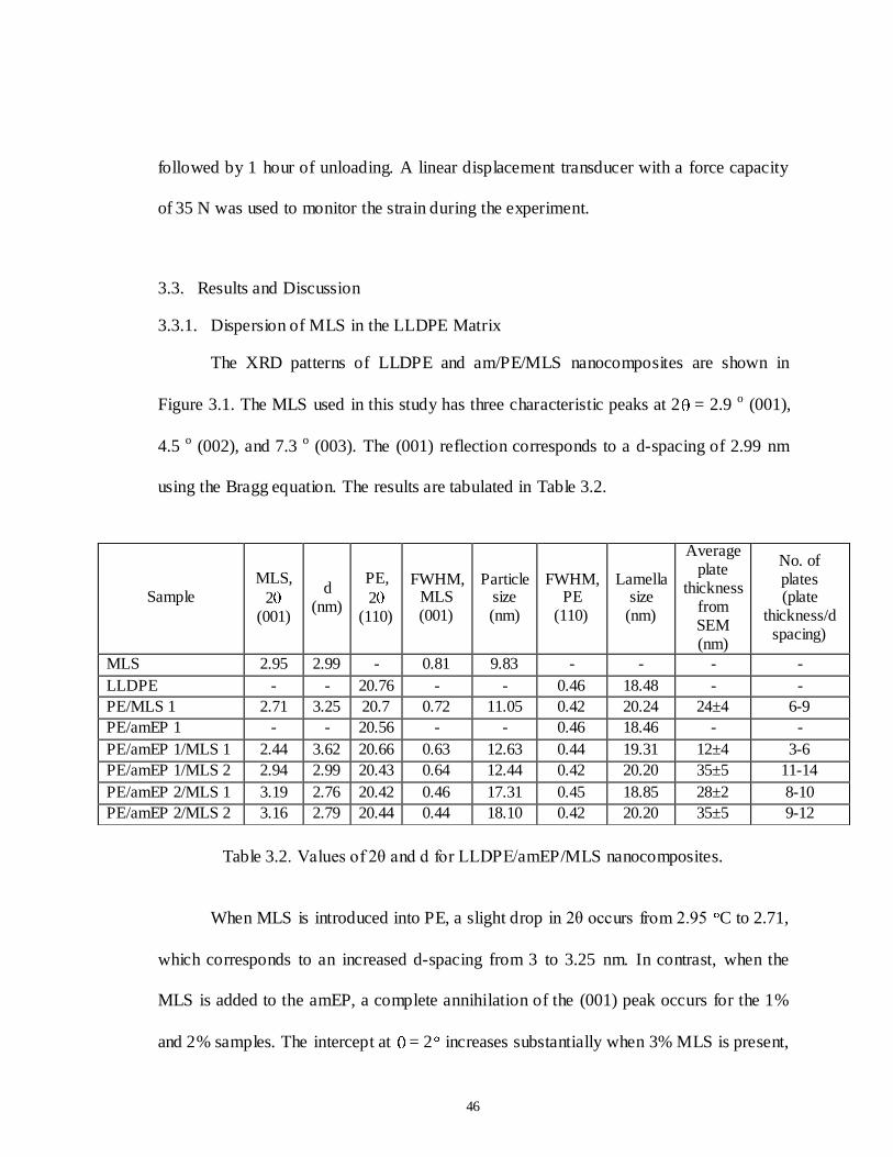
46
followed by 1 hour of unloading. A linear displacement transducer with a force capacity
of 35 N was used to monitor the strain during the experiment.
3.3. Results and Discussion
3.3.1. Dispersion of MLS in the LLDPE Matrix
The XRD patterns of LLDPE and am/PE/MLS nanocomposites are shown in
Figure 3.1. The MLS used in this study has three characteristic peaks at 2 = 2.9 o (001),
4.5 o (002), and 7.3 o (003). The (001) reflection corresponds to a d-spacing of 2.99 nm
using the Bragg equation. The results are tabulated in Table 3.2.
Table 3.2. Values of 2θ and d for LLDPE/amEP/MLS nanocomposites.
When MLS is introduced into PE, a slight drop in 2θ occurs from 2.95 C to 2.71,
which corresponds to an increased d-spacing from 3 to 3.25 nm. In contrast, when the
MLS is added to the amEP, a complete annihilation of the (001) peak occurs for the 1%
and 2% samples. The intercept at = 2 increases substantially when 3% MLS is present,
Sample MLS,
2 (001)
d (nm)
PE,
2 (110)
FWHM, MLS (001)
Particle size (nm)
FWHM, PE
(110)
Lamella size
(nm)
Average plate
thickness from SEM (nm)
No. of plates (plate
thickness/d spacing)
MLS 2.95 2.99 - 0.81 9.83 - - - -
LLDPE - - 20.76 - - 0.46 18.48 - -
PE/MLS 1 2.71 3.25 20.7 0.72 11.05 0.42 20.24 24±4 6-9
PE/amEP 1 - - 20.56 - - 0.46 18.46 - -
PE/amEP 1/MLS 1 2.44 3.62 20.66 0.63 12.63 0.44 19.31 12±4 3-6
PE/amEP 1/MLS 2 2.94 2.99 20.43 0.64 12.44 0.42 20.20 35±5 11-14
PE/amEP 2/MLS 1 3.19 2.76 20.42 0.46 17.31 0.45 18.85 28±2 8-10
PE/amEP 2/MLS 2 3.16 2.79 20.44 0.44 18.10 0.42 20.20 35±5 9-12
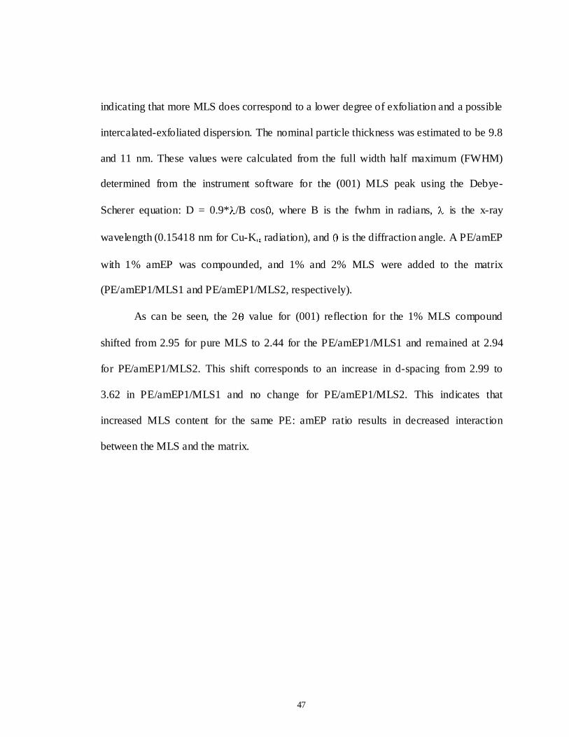
47
indicating that more MLS does correspond to a lower degree of exfoliation and a possible
intercalated-exfoliated dispersion. The nominal particle thickness was estimated to be 9.8
and 11 nm. These values were calculated from the full width half maximum (FWHM)
determined from the instrument software for the (001) MLS peak using the Debye-
Scherer equation: D = 0.9* /B cos , where B is the fwhm in radians, is the x-ray
wavelength (0.15418 nm for Cu-K radiation), and is the diffraction angle. A PE/amEP
with 1% amEP was compounded, and 1% and 2% MLS were added to the matrix
(PE/amEP1/MLS1 and PE/amEP1/MLS2, respectively).
As can be seen, the 2 value for (001) reflection for the 1% MLS compound
shifted from 2.95 for pure MLS to 2.44 for the PE/amEP1/MLS1 and remained at 2.94
for PE/amEP1/MLS2. This shift corresponds to an increase in d-spacing from 2.99 to
3.62 in PE/amEP1/MLS1 and no change for PE/amEP1/MLS2. This indicates that
increased MLS content for the same PE: amEP ratio results in decreased interaction
between the MLS and the matrix.

48
2.5 5.0 7.5 10.0
Arb
itra
ry I
nte
ns
ity
2 (o)
LLDPE
PE/MLS 1
PE/amEP 1
PE/amEP 1/MLS 1
PE/amEP 1/MLS 2
PE/amEP 2/MLS 1
PE/amEP 2/MLS 2
MLS
(a)
10 15 20 25 30
LLDPE
PE/MLS 1
PE/amEP 1
PE/amEP 1/MLS 1
PE/amEP 1/MLS 2
PE/amEP 2/MLS 1
PE/amEP 2/MLS 2
Arb
itra
ry In
ten
sity
2 (o)
(b)
Figure 3.1. XRD patterns of LLDPE and amEP/MLS nanocomposites: (a) MLS (001) reflections, (b) PE (110) reflections.
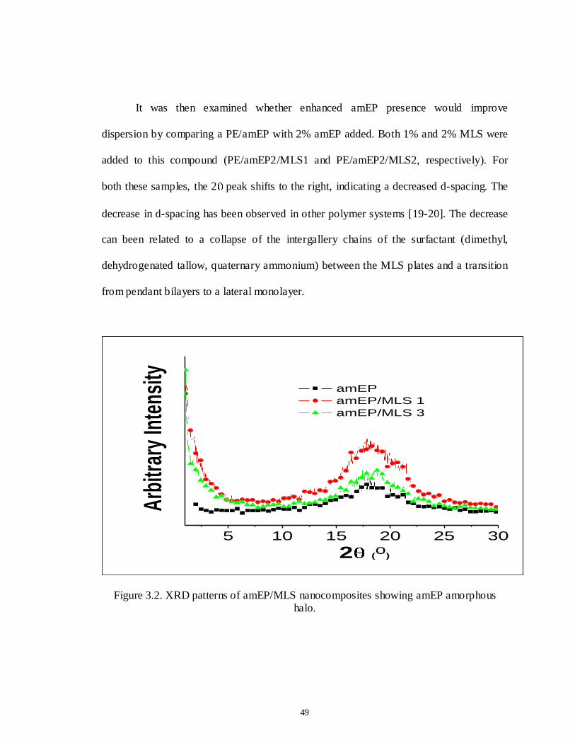
49
It was then examined whether enhanced amEP presence would improve
dispersion by comparing a PE/amEP with 2% amEP added. Both 1% and 2% MLS were
added to this compound (PE/amEP2/MLS1 and PE/amEP2/MLS2, respectively). For
both these samples, the 2 peak shifts to the right, indicating a decreased d-spacing. The
decrease in d-spacing has been observed in other polymer systems [19-20]. The decrease
can been related to a collapse of the intergallery chains of the surfactant (dimethyl,
dehydrogenated tallow, quaternary ammonium) between the MLS plates and a transition
from pendant bilayers to a lateral monolayer.
5 10 15 20 25 30
Arb
itrar
y In
tens
ity
2 (o
)
amEP
amEP/MLS 1
amEP/MLS 3
Figure 3.2. XRD patterns of amEP/MLS nanocomposites showing amEP amorphous halo.

50
The FIB/SEM images of LLDPE nanocomposites in Figure 3.3 show good
dispersion of the stacked platelets. The d spacing of the MLS is 2.99 nm. The average
thickness of the platelets for LLDPE with 1% MLS is 24 ± 4 nm (determined with FEI
Nova software). This thickness indicates that six to nine plates are stacked together. The
addition of 1% amEP reduces the average thickness to 12 ± 4 nm. This reduction in
thickness is an indication that three to six plates are stacked together. The number of
stacked platelets increases for the addition of 2% MLS while keeping the amEP at 1%.
The same increase is observed for the addition of 1% and 2% MLS with 2%
amEP into LLDPE. The average distance between these stacked platelets is 200 ± 50 nm
for the PE with MLS alone, 300 ± 50 nm for the LLDPE/1% amEP/1% MLS, 250 ± 50
nm for the LLDPE/1% amEP/2% MLS, 350 ± 50 nm for the LLDPE/2% amEP/1% MLS,
and 300 ± 50 nm for the LLDPE/2% amEP/2% MLS nanocomposite. Thus, it can be
inferred that while platelet stacking continues, the dispersion of the stacks within the
matrix material is significant and enhanced by the presence of amEP. Figure 3.4 shows
the good dispersion obtained for the addition of 1 and 3% MLS into amEP which further
confirms the synergistic effect of adding amEP into the bulk PE matrix.
The results of dispersion indicate that PE/amEP1/MLS1 provides maximum
dispersion and extent of intercalation in the system.

51
(a)
(b)
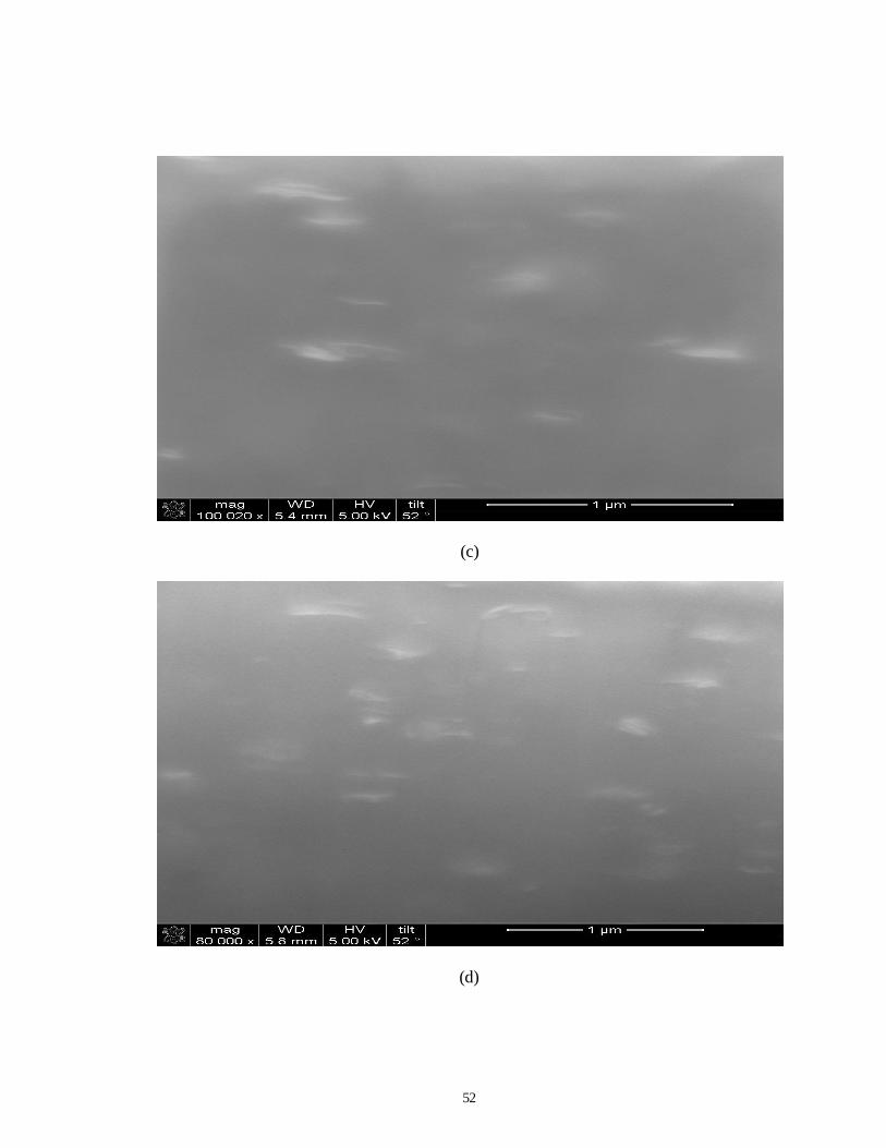
52
(c)
(d)

53
(e)
Figure 3.3. FIB/SEM images of (a) LLDPE/1% MLS nanocomposite, (b) LLDPE/1% amEP/1% MLS, (c) LLDPE/1% amEP/2% MLS, (d) LLDPE/2% amEP/1% MLS, and (e)
LLDPE/2% amEP/2% MLS nanocomposites.
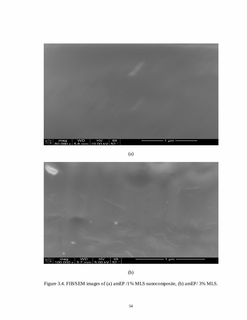
54
(a)
(b)
Figure 3.4. FIB/SEM images of (a) amEP /1% MLS nanocomposite, (b) amEP/ 3% MLS.
55
3.3.2. Crystallization Effects
Crystallization was probed by examining both the XRD peaks of the PE and the
DSC heating and cooling thermograms. XRD results are shown in Figures 3.1 and 3.2.
The (110) reflection of PE is analyzed in Table 3.1.
As it can be seen, the 2 values for the (110) reflections of PE are not affected by
the variations in the PE: amEP ratio or the extent of MLS present in the composites. The
amEP results indicate an amorphous halo corresponding to a peak of 18o 2 . The lamella
thicknesses, however, are affected. When MLS is introduced into PE, a decrease in
FWHM from 0.46 to 0.42 corresponds to an increase in lamella thickness from about 18
to 22 nm. Blending amEP into PE shows no impact on lamella thicknesses. The PE/amEP
with 1% amEP was compounded, and 1% and 2% MLS were added to the matrix
(PE/amEP/MLS1 and PE/amEP/MLS2, respectively). These compositions showed an
increase in lamella thickness with MLS concentration with its being 19 and 20 nm as the
MLS concentration increased from 1% to 2%. Increased maleation served to show similar
trends in crystalline lamella. That is, PE/amEP2/MLS1 and PE/amEP2/MLS2 had the
same changes in lamella thicknesses as PE/amEP1/MLS1 and PE/amEP2/MLS1 did. It
can be thus concluded that MLS had a small effect on the PE crystallization but that
amEP was not a participant in either the 2-part or 3-part compounds. These results were
complemented by the DSC results.
Figure 3.5 shows the DSC results of the neat LLDPE films and the
nanocomposites. The melting temperature (Tm), enthalpy of melting (ΔHm), melt
crystallization temperature (Tmc), enthalpy of melt crystallization (ΔHmc), and the
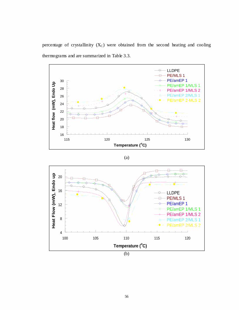
56
percentage of crystallinity (XC) were obtained from the second heating and cooling
thermograms and are summarized in Table 3.3.
16
18
20
22
24
26
28
30
115 120 125 130
LLDPE
PE/MLS 1
PE/amEP 1
PE/amEP 1/MLS 1
PE/amEP 1/MLS 2
PE/amEP 2/MLS 1
PE/amEP 2-MLS 2
Hea
t fl
ow
(m
W),
En
do
Up
Temperature (oC)
(a)
4
8
12
16
20
100 105 110 115 120
LLDPE
PE/MLS 1PE/amEP 1
PE/amEP 1/MLS 1PE/amEP 1/MLS 2PE/amEP 2/MLS 1
PE/amEP 2/MLS 2Hea
t F
low
(m
W),
En
do
up
Temperature (oC)
(b)
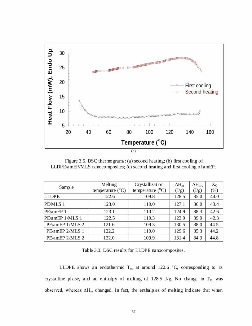
57
5
10
15
20
25
30
20 40 60 80 100 120 140 160
First coolingSecond heating
He
at
Flo
w (
mW
), E
nd
o U
p
Temperature (oC)
(c)
Figure 3.5. DSC thermograms: (a) second heating; (b) first cooling of
LLDPE/amEP/MLS nanocomposites; (c) second heating and first cooling of amEP.
Sample Melting
temperature (oC)
Crystallization
temperature (oC)
ΔHm
(J/g)
ΔHmc
(J/g)
XC
(%)
LLDPE 122.6 109.8 128.5 85.0 44.0
PE/MLS 1 123.0 110.0 127.1 86.0 43.4
PE/amEP 1 123.1 110.2 124.9 88.3 42.6
PE/amEP 1/MLS 1 122.5 110.3 123.9 89.0 42.3
PE/amEP 1/MLS 2 121.6 109.3 130.5 88.0 44.5
PE/amEP 2/MLS 1 122.2 110.0 129.6 85.3 44.2
PE/amEP 2/MLS 2 122.0 109.9 131.4 84.3 44.8
Table 3.3. DSC results for LLDPE nanocomposites.
LLDPE shows an endothermic Tm at around 122.6 oC, corresponding to its
crystalline phase, and an enthalpy of melting of 128.5 J/g. No change in Tm was
observed, whereas ΔHm changed. In fact, the enthalpies of melting indicate that when

58
amEP and MLS are individually added to PE, the enthalpies of melting are lower than
that of the nanocomposite containing both additives. This change indicates a smaller
distribution of crystallite sizes for these nanocomposites.
The cooling thermogram of the neat LLDPE shows an exothermic peak at around
109.8 oC, which corresponds to Tmc and a melt crystallization enthalpy of 85 J/g. Tmc
stayed the same, whereas ΔHmc changed. Indeed, the enthalpy of crystallization shows a
small increase when MLS and amEP were added separately and in combination at ratios
of 1:1 and 1:2 (amEP: MLS). A decrease in ΔHmc was observed in the nanocomposites
having amEP and MLS ratios of 2:1 and 2:2.
The degree of crystallinity of the neat LLDPE and the nanocomposites was
calculated according to the relation Xc = ΔHm/ΔHmo, where ΔHmo is the equilibrium heat
of fusion of PE which was taken as 293 J/g [16].The overall crystallinity does not change,
which suggests that MLS does not act as a nucleating site in the LLDPE matrix and
negates the possibility that increased crystallinity could be responsible for the improved
mechanical properties.
3.3.3. Tensile Stress-Strain Results
A stress-strain curve of LLDPE nanocomposites at room temperature is shown in
Figure 3.6. The tensile properties, which include yield stress and Young’s modulus, are
tabulated in Table 3.4. The decreased crystallinity of the PE resin used in this study is
reflected in the modulus value of 0.12 GPa compared to the value of 0.58 GPa previously
reported [16].
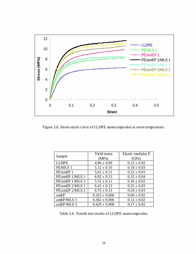
59
0
2
4
6
8
10
12
0 0.1 0.2 0.3 0.4 0.5
LLDPE
PE/MLS 1
PE/amEP 1
PE/amEP 1/MLS 1
PE/amEP 1/MLS 2
PE/amEP 2/MLS 1
PE/amEP 2/MLS 2
Str
es
s (
MP
a)
Strain
Figure 3.6. Stress-strain curve of LLDPE nanocomposites at room temperature.
Sample Yield stress
(MPa)
Elastic modulus E
(GPa)
LLDPE 4.86 ± 0.09 0.12 ± 0.02
PE/MLS 1 5.12 ± 0.10 0.18 ± 0.03
PE/amEP 1 5.61 ± 0.11 0.22 ± 0.03
PE/amEP 1/MLS 1 6.92 ± 0.13 0.32 ± 0.04
PE/amEP 1/MLS 2 5.51 ± 0.11 0.16 ± 0.02
PE/amEP 2/MLS 1 6.41 ± 0.12 0.25 ± 0.03
PE/amEP 2/MLS 2 6.75 ± 0.13 0.24 ± 0.03
amEP 0.325 ± 0.006 0.09 ± 0.02
amEP/MLS 1 0.362 ± 0.006 0.12 ± 0.02
amEP/MLS 3 0.429 ± 0.008 0.17 ± 0.02
Table 3.4. Tensile test results of LLDPE nanocomposites.

60
There is a noticeable increase in yield stress and elastic modulus when MLS is
added to the PE matrix (Figure 3.6). The addition of 1% amEP resulted in an 80%
increase in elastic modulus, whereas the addition of 1% MLS caused an increase of 50%.
Adding 1% amEP/2% MLS, 2% amEP/1% MLS, and 2% amEP/2% MLS in LLDPE
caused increases of 33, 108, and 100% in modulus, respectively. The highest increases in
elastic modulus (166%) are for samples in which a combination of 1% amEP and 1%
MLS is used. The yield stress values follow the same trends as observed in the elastic
modulus. The yield stress increased from 4.86 MPa for neat PE to 6.92 MPa for the
LLDPE/1% and amEP/1% MLS. The yield stress and modulus of 1% amEP/2% MLS,
2% amEP/1% MLS, and 2% amEP/2% MLS into LLDPE also shows a significant
increase compared to the neat PE. This increase indicates the combined effect of amEP
and MLS, which is distinct from a previous report [18] in the positive impact that amEP
has on the PE matrix.
Figure 3.7 shows the effect of adding MLS to the amEP in an approach to
separate the effect of adding MLS and the amEP in combination and separately to the
LLDPE matrix. The addition of 1% MLS to amEP increases the yield stress and elastic
modulus by 10% and 12 %, respectively. An increase of 35% and 90 % is observed with
the addition of 3% MLS. The results, which are presented in Table 3.4, show that MLS
has a similar effect on amEP and LLDPE, suggesting the significant role of MLS as an
effective nanofiller in the LLDPE nanocomposites.

61
It is clear, therefore, that all maleated LLDPE nanocomposites show an increase
in the tensile properties compared to the neat PE. The results also highlight the
synergistic effect of adding amEP and MLS together.
0
0.125
0.25
0.375
0.5
0 0.5 1 1.5 2
amEP
amEP/MLS 1
amEP/MLS 3
Str
es
s (
MP
a)
Strain
Figure 3.7. Stress-strain curve of amEP/MLS nanocomposites at room temperature.
3.3.4. Creep Response
Figure 3.8 shows the creep-recovery curves of LLDPE/amEP/MLS
nanocomposites at room temperature. The stress level applied is 50% of yield stress. All
samples showed an irrecoverable permanent deformation although the applied load was
well within the linear region. When MLS is added, the creep compliance decreases and
the material recovers more. This decrease can be explained by the addition of an elastic

62
component (MLS), which gives the matrix its stiffness (less creep) and elasticity (more
recovery). The addition of the elastomeric amEP improves the recovery in the
LLDPE/amEP blend. The creep compliance further decreases with the addition of 1%
amEP/2% MLS, 2% amEP/1% MLS, and 2% amEP/2% MLS into LLDPE.
0
0.05
0.1
0.15
0.2
0 1000 2000 3000 4000 5000 6000 7000 8000
LLDPE
PE/MLS 1
PE/amEP 1
PE/amEP 1/MLS 1
PE/amEP 1/MLS 2
PE/amEP 2/MLS 1
PE/amEP 2/MLS 2
Cre
ep
Co
mp
lia
nc
e (
GP
a-1
)
Time (sec)
Figure 3.8. Creep-recovery curves of LLDPE/amEP/MLS nanocomposites at room temperature.
When a combination of 1% amEP and 1% MLS is added, the material shows the
lowest creep compliance and the lowest unrecoverable deformation, as shown in Figure
3.8. This behavior mirrors the tensile test results in which LLDPE/1% amEP/1% MLS
films show the highest yield stress and modulus (Table 3.4).
To study the effect of the different components on the viscoelastic response of
LLDPE nanocomposites, 1% and 3% MLS were added to the amEP matrix. Figure 3.9
shows a creep-recovery plot of amEP/MLS nanocomposites. The addition of 1% MLS

63
causes amEP to have lower creep compliance, and the amount of recovery increases from
72% to 75%. Increasing the concentration of MLS to 3% further decreases the creep
compliance, and the amount of recovery shows a noticeable increase to 85%. It is clear,
then, that MLS improves creep resistance and acts as a damping material in both amEP
and LLDPE nanocomposites.
0
1
2
3
4
0 1000 2000 3000 4000 5000 6000 7000 8000
amEPamEP/MLS 1
amEP/MLS 3
Cre
ep
Co
mp
lian
ce
(G
Pa
-1)
Time (sec)
Figure 3. 9. Creep-recovery curves of amEP/MLS nanocomposites at room temperature.
These effects are shown by analyzing the recovery and creep curves and applying
a Lai and Baker approach [ 21]. In linear viscoelasticity,
)()(arac
tttt
where εc and εr are the creep and recovery strains, respectively; and ta is the time at
unloading. The comparison between creep and recovery is shown schematically in Figure
3.10 with εp as the unrecovered plastic strain.

64
r
p
Str
ain
Time
c
ta
Figure 3.10. Creep-recovery schematic.
If the strain is completely recoverable after removal of the applied load, the
recovered strain should coincide with the recovered strain from creep. However, if the
material behaves in a non- linear viscoelastic manner, εc(t-ta) doesn’t coincide with εr(t-
ta) after the load is removed. Divergence of the creep strain from the creep strain shows
that an irrecoverable plastic strain is produced by the applied load. Lai and Baker [21]
applied this concept to high-density polyethylene (HDPE) at different low-stress levels.
Divergence of the creep strain from the recovered strain was observed for HDPE
at low stress levels and was correlated to the strong non- linearity of the material.
Drozdov and Christiansen [22] also predicted that viscoplasticity is restricted in polymer
nanocomposites. They suggested that the applied load produces an irrecoverable plastic
strain. Figure 3.11 shows the comparison of creep and recovery compliance of LLDPE
and its nanocomposites at room temperature. It can be seen that the recovered compliance

65
does not coincide with creep compliance. Divergence of the recovery strain from the
creep strain suggests that an irrecoverable deformation exists. Addition of 1% MLS into
LLDPE decreases the degree of divergence. The degree of divergence furthe r decreases
with the addition of 1% amEP to LLDPE. Addition of a combination of amEP and MLS
gives the lowest divergence, which is supported by the increased elasticity observed in
the tensile results of the LLDPE/amEP/MLS combination.
0
0.07
0.1
0.2
0
0.05
0.1
0.15
0.2
0 500 1000 1500 2000 2500 3000 3500 4000
Creep Compliance
Recovery Compliance
Cre
ep
Co
mp
lia
nc
e (
GP
a-1
)
Rec
ov
ery
Co
mp
lain
ce
(GP
a-1)
Time (sec)
(a)
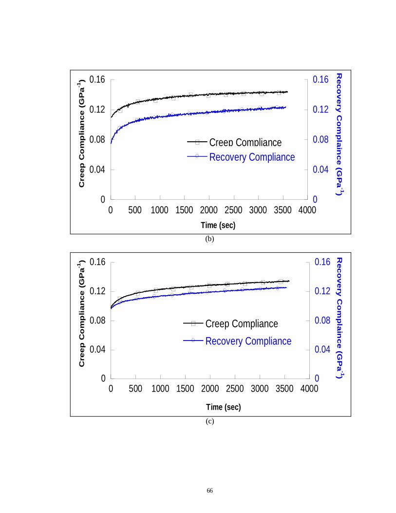
66
0
0.04
0.08
0.12
0.16
0
0.04
0.08
0.12
0.16
0 500 1000 1500 2000 2500 3000 3500 4000
Creep Compliance
Recovery Compliance
Creep
Co
mp
lian
ce (
GP
a-1
)
Reco
very C
om
pla
ince (G
Pa
-1)
Time (sec)
(b)
0
0.04
0.08
0.12
0.16
0
0.04
0.08
0.12
0.16
0 500 1000 1500 2000 2500 3000 3500 4000
Creep Compliance
Recovery Compliance
Cre
ep
Co
mp
lia
nc
e (
GP
a-1
)
Rec
ov
ery
Co
mp
lain
ce
(GP
a-1)
Time (sec)
(c)

67
0
0.03
0.06
0.09
0.1
0
0.03
0.06
0.09
0.12
0 500 1000 1500 2000 2500 3000 3500
Creep Compliance
Recovery Compliance
Creep
Co
mp
lian
ce (
GP
a-1
)
Reco
very C
om
pla
ince (G
Pa
-1)
Time (sec)
(d)
Figure 3.11. Comparison of creep-recovery compliance of LLDPE and its nanocomposites at room temperature: (a) pure LLDPE, (b) LLDPE/1% MLS, (c)
LLDPE/1% amEP, and (d) LLDPE/1% amEP/1% MLS.
To evaluate the changes of the material properties with the addition of amEP and
MLS, Burgers model was used to fit the creep data of the different LLDPE and amEP
nanocomposites. Figure 3.12 shows the experimental and theoretical creep results of
different LLDPE nanocomposites. It is clearly seen that there is agreement between
theoretical and experimental results. The results of the Burgers fit parameters for all
samples are tabulated in Table 3.5.

68
0
0.07
0.1
0.2
1.5 2 2.5 3 3.5 4
PE (Experimental)
PE (Burgers)
PE (KWW)
PE/amPE 1 (Experimental)
PE/amPE 1 (Burgers)
PE/amPE 1 (KWW)
PE/MLS 1 (Experimental)
PE/MLS 1 (Burgers)
PE/MLS 1 (KWW)
PE/amPE 1/MLS 1 (Experimental)PE/amPE 1/MLS 1 (Burgers)PE/amPE 1/MLS 1 (KWW)
Cre
ep
Co
mp
lia
nc
e (
GP
a-1
)
log t (sec)
Figure 3.12. Comparison of experimental data to the Burgers model and the KWW
function.
Sample EM
(109 Pa)
EK
(109 Pa)
ηK
(1011 Pa.s)
ηM
(1012 Pa .s)
τ
(sec)
%
recovery
LLDPE 0.09 0.29 1.52 1.32 528 72
PE/MLS 1 0.08 0.31 1.54 2.75 493 95
PE/amEP 1 0.09 0.52 2.64 3.39 482 88
PE/amEP 1/MLS 1 0.12 0.66 3.53 4.83 472 95
PE/amEP 1/MLS 2 0.10 0.25 1.07 1.42 422 82
PE/amEP 2/MLS 1 0.13 0.40 1.65 1.89 413 80
PE/amEP 2/MLS 2 0.14 0.65 2.72 1.94 418 85
amEP 0.64 0.95 7.50 1.70 690 72
amEP/MLS 1 0.79 1.07 8.49 2.73 621 75
amEP/MLS 3 0.86 1.32 10.51 3.83 597 85
Table 3.5. Burgers fit parameters of LLDPE nanocomposites.

69
According to the Burgers constitutive equation, the modulus EM of the Maxwell
spring determined the instantaneous elastic creep strain, which could be immediately
recovered on the removal of stress. In general, the nanocomposites showed higher values
of EM compared to neat matrix. Among the nanocomposites, LLDPE/amEP 1/MLS 1
behaved with the highest elasticity. In the case of LLDPE/MLS systems, the nanoclay
layers could bear load because of the large aspect ratio of the individual platelet while
discounted by the slippage of stacks and large amount of unexfoliated layers. Hence, the
resulting EM of LLDPE/amEP 1/MLS 1 was higher than the neat matrix. This increase
reflects the tensile test results in which the nanocomposites with amEP and MLS had
higher yield stress and modulus (Table 3.5). The instantaneous elasticity EM reasonably
corresponded to the elasticity of the crystalline part of the polymer, which took the
immediate load because of high stiffness compared to the amorphous polymer. The
crystallinity of each specimen was not obviously altered with the addition of the MLS
particles, which implied that the load bearing parts were not greatly different between the
neat LLDPE matrix and the nanocomposites.
The time-dependent EK and ηK in the Kelvin unit might be associated with the
stiffness and viscous or oriented flow of amorphous polymer chains in short term,
respectively. EK and ηK of the nanocomposites increased considerably with the addition
of amEP and MLS. The addition of 1% amEP and 1% MLS showed a maximum in these
values. The materials with a relatively higher bulk modulus deformed very little, and the
Kelvin unit behaved with a higher modulus and very difficult viscous flow. EK and ηK of
the neat PE showed a small change with the addition of 2% MLS while keeping amEP at

70
1%, whereas an increase is observed with the addition of 1% and 2% MLS with 2%
amEP into LLDPE. The addition of amEP and MLS showed reinforcement effectiveness
on the Kelvin unit and showed to be effective to retard the deformation of the Kelvin
unit.
EK and ηK were used to determine the retardation time. Ideal elastic materials
display an immediate recovery after loading and subsequent removal of the load. In the
case of viscoelastic materials, there is a time delay for recovery. The retardation time is
the delayed response to an applied force or stress. Figure 3.13 shows the retardation time
behavior of LLDPE nanocomposites.

71
0
100
200
300
400
500
600
700
800
τ Burg
ers (
sec)
Figure 3.13. Burgers retardation time comparison of LLDPE and amEP nanocomposites.
The retardation time decreases from 528 sec for LLDPE to 493 sec with the
addition of 1% amEP. The addition of 1% MLS further decreases the retardation time.
Adding a combination of amEP and MLS with different ratios into LLDPE gives smaller
retardation times. The results show that both EM and retardation time reflect the final
percentage recovery of LLDPE nanocomposites.
Another important parameter to consider in the Burgers constitutive equation is
ηM that describes the irrecoverable creep as compared to the instantaneous and time-
dependent parameters that showed enhancement with the addition of amEP and MLS.
From Table 3.5, it can be seen that ηM increases with the addition of amEP and MLS. It
can be considered that ηM is associated with the damage from crystallized polymer or
oriented noncrystalline regions, such as the pulling out of chain folds by a crystal slip
process and the breaking of an intercrystalline tie molecule or the irreversible
72
deformation from amorphous regions, such as breaking of bridging segments between the
clay particles and the polymer chains. The enhanced resistance to deformation was
obtained with the addition of amEP and MLS. Addition of 1% of amEP and 1% MLS
separately or combined increases ηM reflecting the fact of a decrement of the
irrecoverable deformation. The results are reflected in the higher % recovery for the
composites containing 1% amEP and 1% MLS. Addition of 2% MLS while keeping
amEP at 1% shows lower ηM values indicating an increase in the amount irrecoverable
deformation and hence a lower % recovery value. The results can be attributed to the ease
of mobility of the polymer chains.
To assess both the retardation time and the breadth of relaxation times, creep
compliance curves were fitted with the KWW [23-24] stretched exponential function
])/exp(1[)( 0 tDtD
where D(t) is the creep compliance, τ is the characteristic retardation time, and β is a
creep shape parameter. The numerical analysis of the creep compliance curve fits was
performed using OriginLab™ nonlinear least-squares data analysis software.
Figures 3.13 and 3.14 compare the KWW fit parameters of LLDPE and amEP
nanocomposites. A retardation time represents resistance offered by the microstructure to
the elastic deformation of the system. As the retardation time decreases (i.e., as less
resistance occurs), the system response becomes more elastic. The results of the sample
investigated are tabulated in Table 3.6.

73
0.0
0.2
0.4
0.6
0.8
1.0
1.2
1.4
1.6
τk
ww
(se
c)
Figure 3.14. Retardation time comparison of LLDPE and amEP nanocomposites.
0.0
0.2
0.4
0.6
0.8
1.0
1.2
βkw
w
Figure 3.15. Comparison of βkww for the different LLDPE and amEP nanocomposites.

74
Sample τkww(sec) βkww
LLDPE 1.47 0.50
PE/MLS 1 0.89 0.21
PE/amEP 1 0.93 0.19
PE/amEP 1/MLS 1 0.86 0.21
PE/amEP 1/M LS 2 0.96 0.20
PE/amEP 2/MLS 1 0.92 0.19
PE/amEP 2/MLS 2 0.92 0.18
amEP 1.43 1.08
amEP/MLS 1 1.11 1.00
amEP/MLS 3 0.86 0.89
Table 3.6. KWW curve fitting parameters.
Pure LLDPE and amEP had a similar retardation time at room temperature. The
breadth of the relaxations, which are inversely related to β, show that the LLDPE had a
larger breadth than the amEP. For LLDPE nanocomposites, the addition of 1% MLS
decreases the retardation time from 1.47 sec for LLDPE to 0.89 sec for PE/1% MLS. For
amEP nanocomposites, the addition of 1% MLS also causes a decrease in the retardation
time. The retardation time decreases from 1.43 sec for amEP to 1.11 sec for amEP/1%
MLS. The addition of 3% MLS to amEP further decreases the retardation time to 0.86
sec. The results can be explained by the addition of the rigid MLS particles, which act to
increase the elasticity of the matrix and hence reduce the retardation time. The retardation
time increases to 0.93 when 1% amEP is used. The corresponding effect on the breadth of
relaxations indicates that the effect on the LLDPE is to increase it substantially, whereas
marginal impact on relaxation breadth is obtained in the amEP + MLS composites. The
combined nanocomposites based on both LLDPE and amEP show values similar to those

75
obtained in the PE +MLS systems. The values of β remained constant (β = 0.19 ± 0.02)
despite the different amounts of MLS and amEP that have been added into the PE matrix.
For amEP nanocomposites, the β values decrease from 1.08 for neat amEP to 1
and 0.89 with the addition of 1% and 3% MLS to amEP, respectively. A decrease in the β
parameter can be interpreted as a strengthening of the coupling between the relaxing
species and the medium and is related to an overall decrease of the molecular mobility. A
minimum in the values of retardation time is obtained when a combination of 1% MLS
and 1% amEP is used. The addition of 2% amEP with 1% and 2% MLS to PE retains the
value of 0.92 sec for the retardation time. The results obtained for LLDPE
nanocomposites suggest that a combination of 1%MLS and 1% amEP gives the lowest
retardation time. The enhanced recovery observed for the combination of amEP and MLS
is reflected in lower τ values. We note that the addition of MLS to either PE or amEP
influences retardation time and relaxation breadth. We also note that the blend of LLDPE
+ amEP indicates a larger relaxation breadth and a decrease in retardation time of the
pure PE and amEP.
3.4. Error Analysis
All experiments were validated as follows:
For DSC, a set of two samples were used to ensure reproducibility of the data.
Enthalpies of melting and crystallization were calculated using the Pyris software on the
Perkin Elmer DSC6.

76
For XRD, a set of two samples were used to ensure reproducibility of the data.
The 2 theta values, the d spacing, and the FWHM were calculated using the Rigaku
Ultima III software.
For Tensile testing, a total of five samples were tested according to ASTM D882.
Figure 3.16 shows a representative curve for tensile test of LLDPE showing the overlay
of three samples. The error analysis was presented in Table 3.4. The yield stress was
calculated as the deviation of the stress from the linear region on the stress-strain curve.
For creep testing, two samples were used to ensure reproducibility of the data.
The creep compliance was calculated as the ratio of the strain obtained from RSA III
software divided by the constant stress applied during the creep test.
0
1
2
3
4
5
6
7
0 0.05 0.1 0.15 0.2 0.25 0.3 0.35 0.4
Sample 1Sample 2Sample 3S
tres
s (
MP
a)
Strain
(a)

77
0.06
0.08
0.1
0.12
0.14
0.16
0.18
0.2
0 900 1800 2700 3600 4500 5400 6300 7200
Sample 1Sample 2
Cre
ep
Co
mp
lain
ce
(G
Pa
-1)
Time (sec)
(b)
5
10
15
20
25
30
40 60 80 100 120 140 160
Sample 1-Second heatingSample 2-Second heating Sample 1-First cooling Sample 2-First cooling
Hea
t F
low
(m
W),
En
do
Up
Temperature (oC)
(c)
Figure 3.16. Error analysis showing overly of (a) tensile test; (b) creep test; (c) DSC test for pure LLDPE samples.

78
3.5. Conclusions XRD and microscopy of LLDPE nanocomposite films showed some intercalation
effects for samples in which a combination of 1% amEP and 1% MLS was used. An
increase in the interlayer distance was observed for this sample. The amEP proved to be
an effective factor in the dispersion behavior of the nanocomposites and resulted in
improved tensile and creep properties.
Both the Burgers model and the KWW relation model creep behavior (Figure
3.12). The trends in retardation time were more clearly depicted in the KWW relation.
The LLDPE nanocomposite showed a nonlinear viscoelastic behavior. A permanent
deformation was observed in all systems with LLDPE nanocomposite having the lowest
creep. Struik [25] proposed that since the polymer chains adhere to the filler particles, the
segmental mobility near the particles’ surface would be reduced. Far from the particles,
the mobility of the matrix will be similar; thus, a distinction between “disturbed” and
“undisturbed” regions is made. Lai and Baker [21] used this network model to understand
the mechanism of plastic deformation in HDPE at low stress levels. The model assumes
that the time-dependent behavior of a semicrystalline or filled polymer is due to the
amorphous phase only and that crystals do not contribute to viscoelasticity of the polymer
and act as inert fillers or crosslinks behaving elastically. On application of a load, the
deformation from the disturbed amorphous regions and the crystals is recoverable. The
undisturbed amorphous regions undergo an irrecoverable deformation. This behavior can
be seen in the LLDPE/amEP/MLS nanocomposites. The percentage recovery in
LLDPE/amEP/MLS nanocomposites is higher than that of pure LLDPE. This suggests
the role of MLS particles in the absence of crystallites. MLS particles act as hinges in the
79
amorphous matrix; this action is reflected in higher modulus, higher yield strain, and
more recovery. MLS lowers retardation time in all materials but the crystallinity in the
host matrix acts in a similar way. For the pure amorphous material with MLS, the
retardation time values are higher (recovery is lower) as compared to the PE+ amEP
+MLS, in which a higher recovery and a lower retardation time are experienced. The
relaxation breadth is increased when MLS was added to either PE or amEP.
3.6. References
1. K.K. Maniar., Polymer-Plastics Tech. and Eng., 43, 427-443 (2004).
2. F. Hussain, M. Hojati, M. Okamoto, and R. Gorga, J. Composite Materials, 40, 1511-
1575 (2006).
3. J.L. Rand, D.A. Grant, and T. Strganac, AIAA 34th Aerospace Sciences Meeting and
Exhibit (1996).
4. J.L. Rand and W.J. Sterling, 35th COSPAR Scientific Assembly; Adv. Space
Research, Paris (2004).
5. D. Martin, P. Halley, R. Truss, M. Murphy, O. Jackson, and O.Y. Kwon, Polym Int, ,
pp. 1774-1779 (2003).
6. G. Liang, J. Xu, S. Bao, and W. Xu , J. Appl. Polym. Sci., 91, 3974-3980 (2004).
7. G. Malucelli, S. Ronchetti, N. Lak, A. Priola, N.T. Dintcheva, and F.P. La Manta, Eur.
Polym. J., 43, 328-335 (2007).
8. H. Wang, D.G. Thompson, J.R. Schoonover, S.R. Aubuchon, and R.A. Palmer,
Macromolecules, 34, 7084-7090 (2001).
9. M.L. Quintinilla, S.S. Valdez, L.F. Ramos, and R.G. Miranda, Polym. Bulle tin, pp.
385-393 (2006).
10. A. Lee and D. Lichtenhan, J. Appl. Polym. Sci., 73, 1993-2001 (1999).
11. A. Pegoretti, J. Kolarik, C. Peroni, and Cilgiaresi, Polym., 4, 2751-2759 (2004).

80
12. J. Morawiec, A. Pawlak, M. Slouf, A. Galeski, E. Piorkowska, and N. Kransikowa,
Eur. Polym. J., 41, 1115-1122 (2005).
13. R.W. Truss and T.K. Yeow, J. Appl. Polym. Sci., 100, 3044-3049 (2006).
14. J.L. Yang, Z. Zhang, A. Schlarb, and K. Friedrich, Polym., 47, 2791-2801 (2006).
15. U. Gurmendi, J.I. Eqiazabal, and J. Nazabal, Macromol. Mater. Eng., 292, 169-175
(2007).
16. F.C. Chiu, Q. Wang, Q. Fu, P. Honigfort, S. Cheng, B.S. Hsiao, F. Yeh, M.Y.
Keating, E.T. Hsieh, and C.C. Tso, J. Macromolecular Sci., Part B, 39, 317-331 (2000).
17. M. Niaounakis and E. Kontou, J. Polym. Sci.: Part B: Polymer Physics, 43, 1712-
1727 (2005).
18. A. Ranade, K. Nayak, D. Fairbrother, and N.A. D’Souza, Polym, 46, 7323-7333
(2005).
19. Z. Shen, G.P. Simon, and Y.B. Cheng, Polym, 43, 4251-4260 (2002). 20. M. Costache, M.J. Heidecker, E. Manias, and C. Wilkie, Polym. Adv. Technol., 17, 764-771 (2006).
21. L. Lai and A. Bakker, Scripta Metallurgica et Materialia, 28, 1447-1452 (1993).
22. A.D. Drozdov and J. Christiansen, Eur. Polym., 43, 10-25 (2007).
23. F. Kohlrausch, Pogg. Ann Physics, 12, 393 (1847).
24. G. Williams, D.C. Watts, Trans Faraday Soc, 66, 80 (1970).
25. LCE Struik , Physical aging in amorphous polymers and other materials; Elsevier:
New York (1978)

81
CHAPTER 4
EFFECT OF TEMPERATURE ON MOLECULAR RELAXATIONS IN
POLYETHYLENE NANOCOMPOSITES
4.1. Introduction
Polymer nanocomposites are hybrid materials composed of an organic polymer
matrix in which organic fillers with nanoscale dimensions are embedded. The inorganic
fillers dramatically improve the physical and mechanical properties of the polymer [1-4].
For these materials, the ability to model viscoelastic response determines the
understanding of deformation mechanisms and facilitates solutions to their long-term
performance.
Mechanical analogs are commonly used to model long-term performance, the
simplest being the Maxwell model (spring and dashpot in series) and the Voigt model
(spring and dashpot in parallel). The Maxwell model is commonly used for representation
of stress relaxation, whereas the Voigt model is used for creep and recovery
representation. More complex models involve three or four elements, such as the Burgers
model, which is a combination of the Maxwell and Voigt models and can be used for
creep and recovery representation [5].
Creep behavior is an important property of polymer nanocomposites that controls
the dimensional stability, especially in applications where the material supports loads for
long periods [6-11]. This mechanism can cause undesirable deformation that leads to
structural failure. Yang et al. [7] investigated the creep behavior of polyamide 66 (PA66)
nanocomposites at various temperatures for use in aviation and automotive applications.

82
The creep deformation and the creep rate of the matrix were reduced by the
addition of the nanofillers. Ranade et al. [8] studied the potential use of linear low-density
polyethylene (LLDPE) nanocomposites based on montmorillonite-layered silicates
(MLS) as load bearing materials for stratospheric scientific balloons. The creep resistance
and modulus of the polymer was increased by the incorporation of the layered silicate.
The results were attributed to the dispersion effects due to the presence of MLS. Nunez et
al. [9] analyzed the creep properties of polypropylene (PP) composites prepared from
wood flour at different temperatures for use in industrial applications such as automotive
components and domestic appliances. The effect of filler content, addition of
compatibilizing agent, and temperature was investigated. The Burgers model was found
to give a good description of the viscoelastic behavior. The parameters were found from
best-fitting of experimental data. The results showed that the creep deformation
decreased when wood flour concentration was increased. The addition of a small amount
of maleated PP greatly improved creep behavior. The composite showed a strong
dependence of the creep behavior on temperature; the Maxwell modulus E0 showed a
reduction with increasing temperature as a result of material softening.
Morphology plays an important role in the creep behavior of real polymeric
systems. For amorphous polymers, creep behavior can be represented by the Kohlrausch-
Williams-Watts (KWW) function, which states that creep compliance increases according
to a stretched exponential function. The KWW function can be also used for creep
characterization of semicrystalline polymers [12-13]. McKenna et al. [12] studied the
effect of physical aging on the creep behavior of syndiotactic polystyrene (sPS) by using

83
the KWW function. The effect of aging time and temperature was considered. Cheriere et
al. [13] studied the three stages of creep of polymethyl-methacrylate (PMMA) between
55 and 90 oC. After stress application, creep starts by a logarithmic function. It is
followed by a KWW creep stage with an exponent of 0.36. The third stage follows a
power law with an exponent of 0.8.
In our previous experimental studies, the creep behavior of maleated and non-
maleated LLDPE nanocomposites at room temperature was studied [14]. Creep
compliance was significantly reduced with the addition of different ratio of an amorphous
maleated polyethylene (amEP) and MLS. The results were attributed to the good
dispersion of MLS particles which was facilitated by the addition of the compatibilizer.
In this chapter, the modeling of creep behavior by using traditional creep models was
conducted. An attempt to understand the structure-property relationship was carried out
by analyzing the parameters of the Burgers model since variations in these parameters
illustrate the influence of nanofillers on the creep performance of the bulk matrix.
Moreover, the distribution of retardation time was considered by using the KWW
function.

84
4.2. Experimental
4.2.1. Sample Preparation
Nanocomposites were compounded by using a Haake TW100 twin-screw
extruder with a temperature profile of 200, 200, 205, and 210 oC for zones 1 to 4,
respectively. PE films 1.5 mil (0.04 mm) thick were processed with a Killion single-
screw extruder (L/D = 24:1), fitted with a dual- lip air ring and a die diameter of 2 inches.
Blends of PE + amEP + MLS were made, and the mixtures were compounded and
pelletized. The compounded pellets were then extruded into blown films. Table 4.1
summarizes the concentrations used.
Sample LLDPE (wt %)
Exxelor VA 1803 (wt %)
MLS (wt %)
LLDPE 100 0 0
PE/MLS 1 99 0 1
PE/amEP 1 99 1 0
PE/amEP 1/MLS 1 98 1 1
Table 4.1. Summary of concentrations used.
4.2.2. Dynamic Mechanical Analysis (DMA)
DMA experiments were performed with a rheometric solids analyzer (RSA III)
instrument (TA instruments Inc.). The mode of deformation applied is tension, and the
mean sample dimensions are 5 mm × 25 mm with a mean thickness of 40 µm. The
temperature ranged from -100 oC to 100 oC at a heating rate of 3 oC/min, and the
frequency was set at 1 Hz. The storage and loss modulus as well as tan δ versus

85
temperature were evaluated as described in ASTM D5026 (standard test method for
plastics: dynamic mechanical properties in tension).
4.2.3. Tensile Testing
Yield stress, ultimate tensile strength (UTS), and elastic modulus E were
determined by using RSA III film fixture with an extension rate of 0.208 mm/min. The
effect of temperature was studied by running experiments at different temperatures of 25,
10, -10, -30, -50, -70, -90, and -100 oC. A convection oven with a temperature range of -
150 oC to 600 oC was used for this purpose.
4.2.4. Creep Testing
Uniaxial tensile creep tests were performed by using the RSA III with a film
attachment. The desired constant stress to be applied for each measurement was
calculated to be 50% of the yield stress. The constant stress was applied for 1 hour of
loading followed by 1 hour of unloading. A linear displacement transducer with a force
capacity of 35 N was used to monitor the strain during the experiment. Creep tests were
also performed at the same set of temperatures as the tensile tests, and the liquid nitrogen
controller connected to the environmental chamber was used for cooling.
4.3. Results and Discussion
4.3.1. DMA Results
LLDPE usually shows three transition temperatures in DMA designated as α, β,
and γ, which are best obtained from tan δ curve. The α transition ranges from 0 to 120 oC,

86
the β-transition ranges from -30 to 10 oC, and the γ transition ranges from -150 to -120
oC. For the temperature range tested, all samples showed a β transition at around -30 oC
and an α transition between 50 and 60 oC. The transition temperatures and relative change
in magnitude of the E’, E” and tan δ corresponding to the β and α transitions for the
different compositions are shown in Figure 4.1, and the results are tabulated in Table 4.2.
0
5 108
1 109
2 109
2 109
3 109
-80 -40 0 40 80
LLDPE
PE/MLS 1
PE/amEP 1
PE/amEP 1/MLS 1E'
(Pa
)
Temperature (oC)
(a)

87
0
2 107
4 107
6 107
8 107
1 108
-100 -50 0 50 100 150
LLDPEPE/MLS 1 PE/amEP 1PE/amEP 1/MLS 1
E''
(P
a)
Temperature (oC)
(b)
0
0.1
0.2
0.3
-100 -50 0 50 100 150
LLDPEPE/MLS 1PE/amEP 1PE/amEP 1/MLS 1
tan
Temperature (oC)
(c)
Figure 4.1. DMA results showing (a) E’, (b) E”, and (c) tan δ versus temperature of LLDPE nanocomposites.
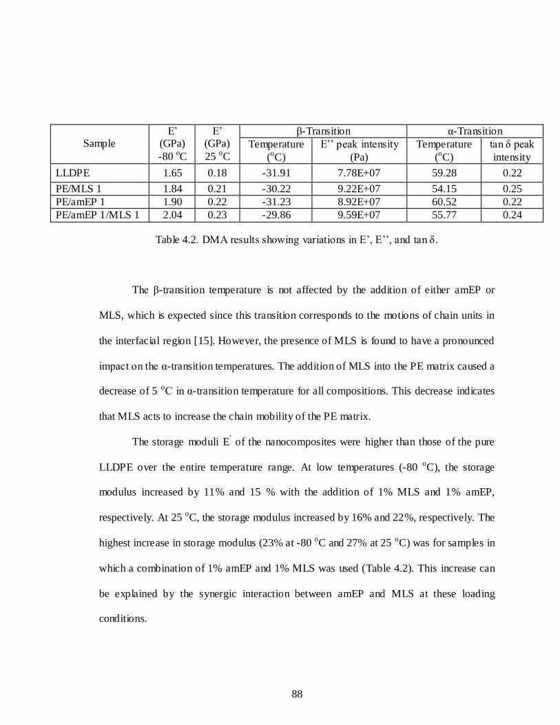
88
Sample E’
(GPa)
-80 oC
E’ (GPa)
25 oC
β-Transition α-Transition
Temperature
(oC)
E’’ peak intensity
(Pa)
Temperature
(oC)
tan δ peak
intensity
LLDPE 1.65 0.18 -31.91 7.78E+07 59.28 0.22
PE/MLS 1 1.84 0.21 -30.22 9.22E+07 54.15 0.25
PE/amEP 1 1.90 0.22 -31.23 8.92E+07 60.52 0.22
PE/amEP 1/MLS 1 2.04 0.23 -29.86 9.59E+07 55.77 0.24
Table 4.2. DMA results showing variations in E’, E’’, and tan δ.
The β-transition temperature is not affected by the addition of either amEP or
MLS, which is expected since this transition corresponds to the motions of chain units in
the interfacial region [15]. However, the presence of MLS is found to have a pronounced
impact on the α-transition temperatures. The addition of MLS into the PE matrix caused a
decrease of 5 oC in α-transition temperature for all compositions. This decrease indicates
that MLS acts to increase the chain mobility of the PE matrix.
The storage moduli E’ of the nanocomposites were higher than those of the pure
LLDPE over the entire temperature range. At low temperatures (-80 oC), the storage
modulus increased by 11% and 15 % with the addition of 1% MLS and 1% amEP,
respectively. At 25 oC, the storage modulus increased by 16% and 22%, respectively. The
highest increase in storage modulus (23% at -80 oC and 27% at 25 oC) was for samples in
which a combination of 1% amEP and 1% MLS was used (Table 4.2). This increase can
be explained by the synergic interaction between amEP and MLS at these loading
conditions.

89
The selection of relative values for E” and tan δ peaks was based on the clarity of
a peak for the β and α transitions, respectively. Adding 1% amEP had a slight impact on
the PE for the β transition. However, the addition of 1% MLS with or without the amEP
increased the peak intensity by 23% and 18%, respectively (Table 4.2). This increase
indicates that the polymer-clay interfacial region played a role in the time response of the
PE. The increases noted in the α-transition peak maxima are even higher. The amEP did
not affect the maxima of the PE for the α transition, indicating no influence on the
amorphous compatibilizer on segmental relaxation. However, the presence of MLS had a
pronounced effect on the maxima, supporting the conclusion that MLS provides an
interface that affects the relaxation in the PE matrix. The change in transition
temperatures and E” peak maxima for composites containing MLS with or without amEP
indicates that the vibrational and orientational motion within the crystals is altered by the
addition of MLS. The increase in E’ and E” values indicates benefits in both the elastic
and the viscous response in the modified PE. The MLS rigid platelets linked to the PE
matrix via the reactive surfactants serve as rigid crystals and can act as anchors in the PE
matrix.
4.3.2. Tensile Test Results
A stress-strain curve of LLDPE nanocomposites at room temperature is shown in
Figure 4.2. The results, which include yield stress and elastic modulus E, are tabulated in
Table 4.3. The decreased crystallinity of the PE resin used is reflected in the modulus
value of 0.12 GPa compared to 0.58 GPa in the previous work [8].

90
The addition of 1% amEP resulted in an 80% increase in modulus, whereas the addition
of MLS caused an increase of 50%. It can be seen that the highest increase in modulus
(166%) occurred for samples in which a combination of 1% amEP and 1% MLS was
used. The yield stress values follow the same trends as observed in the modulus. The
yield stress increased from 4.86 MPa for neat PE to 6.92 MPa for the LLDPE/amEP
1/MLS 1 nanocomposite. This increase indicates the combined effect of amEP and MLS,
which is distinct from the previous work, on the positive impact that amEP has on the PE
matrix.
0
2 106
4 106
6 106
8 106
1 107
1.2 107
0 0.1 0.2 0.3 0.4 0.5
LLDPE
PE/MLS 1
PE/amEP 1
PE/amEP 1/MLS 1
Str
es
s (
Pa
)
Strain
Figure 4.2. Stress-strain curve of LLDPE nanocomposites at room temperature.
The effect of temperature on the tensile properties is important in applications
where temperatures can fall down to -100 oC, particularly in high-altitude balloon films.
Figure 4.3 shows the stress-strain curve of LLDPE and LLDPE/amEP 1/MLS 1 at

91
different temperatures. The results are tabulated in Table 4.3. It is worth mentioning that
all the temperatures showed a similar trend in the stress-strain curves as that observed in
the room temperature measurements.
0
5
10
15
20
25
30
35
0 0.05 0.1 0.15 0.2 0.25 0.3 0.35
25 oC
10 oC
-10 oC
-30 oC
-50 oC
-70 oC
-90 oC
-100 oC
Str
es
s (
MP
a)
Strain
(a)

92
0
5
10
15
20
25
30
35
40
0 0.05 0.1 0.15 0.2 0.25 0.3
25 oC
10 oC
-10 oC
-30 oC
-50 oC
-70 oC
-90 oC
-100 oC
Str
es
s (
MP
a)
Strain
(b)
0
10
20
30
40
50
0 0.05 0.1 0.15 0.2 0.25 0.3
25 oC
10 oC
-10 oC
-30 oC
-50 oC
-70 oC
-90 oC
-100 oC
Str
es
s (
MP
a)
Strain
(c)

93
0
10
20
30
40
50
60
0 0.1 0.2 0.3 0.4
25 oC
10 oC
-10 oC
-30 oC
-50 oC
-70 oC
-90 oC
-100 oC
Str
es
s (
MP
a)
Strain
(d)
Figure 4.3. Stress-strain curve of (a) Pure LLDPE, (b) PE/1% MLS, (c) PE/1% amEP, (d)
PE/1% amEP/1% MLS at different temperatures.

94
Temperature (oC)
Sample Yield stress
(MPa) UTS
(MPa) Elastic modulus E
(GPa)
25
LLDPE 4.86 - 0.12
PE/MLS 1 5.12 - 0.18
PE/amEP 1 5.61 - 0.22
PE/amEP 1/MLS 1 6.92 - 0.32
10
LLDPE 7.01 - 0.15
PE/MLS 1 8.85 - 0.19
PE/amEP 1 9.06 - 0.21
PE/amEP 1/MLS 1 10.3 - 0.26
-10
LLDPE 11.38 - 0.26
PE/MLS 1 10.84 - 0.32
PE/amEP 1 11.67 - 0.38
PE/amEP 1/MLS 1 12.15 - 0.42
-30
LLDPE 14.65 - 0.38
PE/MLS 1 14.92 - 0.57
PE/amEP 1 17.1 - 0.74
PE/amEP 1/MLS 1 19.43 - 0.84
-50
LLDPE 17.86 18.8 0.52
PE/MLS 1 19.87 21.52 0.77
PE/amEP 1 22.34 23.62 0.98
PE/amEP 1/MLS 1 24.3 25.4 1.04
-70
LLDPE 22.84 23.01 0.64
PE/MLS 1 24.90 25.13 0.95
PE/amEP 1 25.39 27.09 1.26
PE/amEP 1/MLS 1 35.51 34.06 1.39
-90
LLDPE 21.18 27.54 1.15
PE/MLS 1 29.57 31.61 1.24
PE/amEP 1 30.34 40.4 1.31
PE/amEP 1/MLS 1 37.1 43.3 1.54
-100
LLDPE 26.02 33.1 1.21
PE/MLS 1 34.84 39.95 1.38
PE/amEP 1 38.57 45.3 1.39
PE/amEP 1/MLS 1 41.64 53.0 1.63
Table 4.3. Tensile test results of LLDPE nanocomposites at different temperatures.
Adding MLS to PE increased the yield stress and the elastic modulus. The
addition of 1% amEP and 1% MLS gave the best performance. At room temperature, the
material exhibited increased work hardening in all samples. As temperatures decreased,

95
the trends in mechanical properties were similar with the LLDPE < PE/MLS 1 <
PE/amEP 1 < PE/amEP 1/MLS 1. A decreased work hardening, however, was evidenced
by a drop in stress following UTS. This change in deformation mechanism occurred for
tests below -50 oC. Below the β transition, an upper and lower yield deformation
reflective of the relaxation processes in the matrix was evident in all samples.
4.3.3. Creep Test Results
Figure 4.4 shows the creep-recovery curves of LLDPE/amEP/MLS
nanocomposites at room temperature. For an elastic material, complete recovery was
obtained. All samples at room temperature showed an irrecoverable permanent
deformation. This deformation explains the non- linear viscoelastic response of the
material. The neat LLDPE showed the highest compliance and the highest permanent
deformation.
0
0.05
0.1
0.15
0.2
0 1000 2000 3000 4000 5000 6000 7000 8000
LLDPE
PE/MLS 1
PE/amEP 1
PE/amEP 1/MLS 1
Cre
ep
Co
mp
lia
nc
e (
GP
a-1
)
Time (sec)
Figure 4.4. Creep-recovery curves of LLDPE nanocomposites at room temperature.

96
When 1% MLS was added, creep compliance decreased and the material showed
more recovery. The addition of an elastic component (MLS) gave the matrix its stiffness
(less creep) and elasticity (more recovery). The addition of the elastomeric amEP
improved the recovery in the LLDPE/amEP 1 blend. When a combination of amEP/MLS
was added to the PE matrix, the material showed the lowest creep compliance and the
lowest unrecoverable deformation. This behavior mirrors the tensile test results where
LLDPE/amEP 1/MLS 1 showed the highest modulus (lowest creep).
The effect of temperature on the creep properties is important in high- altitude
balloons missions. Creep-recovery tests were performed on the LLDPE films at
temperatures as low as -100 oC, which corresponds to high-altitude conditions. Figure 4.5
shows the creep-recovery curves of LLDPE nanocomposites at different temperatures.
The results show the dependence of creep compliance on temperature.

97
0
0.05
0.1
0.15
0.2
0 1000 2000 3000 4000 5000 6000 7000 8000
25 oC
-10 oC
10 oC
-30 oC
-50 oC
-70 oC
-90 oC
-100 oC
Cre
ep
Co
mp
lia
nc
e (
GP
a-1
)
Time (sec)
(a)
0
0.02
0.04
0.06
0.08
0.1
0.12
0.14
0 1000 2000 3000 4000 5000 6000 7000 8000
25oC
10 oC
-10 oC
-30 oC
-50 oC
-70 oC
-90 oC
-100 oC
Cre
ep
Co
mp
lia
nc
e (
GP
a-1
)
Time (sec)
(b)

98
0
0.05
0.1
0.15
0 1000 2000 3000 4000 5000 6000 7000 8000
25 oC
10 oC
-10 oC
-30 oC
-50 oC
-70 oC
-90 oC
-100 oC
Cre
ep
Co
mp
lia
nc
e (
GP
a-1
)
Time (sec)
(c)
0
0.02
0.04
0.06
0.08
0.1
0.12
0 1000 2000 3000 4000 5000 6000 7000 8000
25 oC
10 oC
-10 oC
-30 oC
-50 oC
-70 oC
-90 oC
-100 oC
Cre
ep
Co
mp
lia
nc
e (
GP
a-1
)
Time (sec)
(d)
Figure 4.5. Creep-recovery of LLDPE nanocomposites: (a) pure LLDPE, (b) PE/1%
MLS, (c) PE/1% amEP, (d) PE/1% amEP/1% MLS at different temperatures.

99
4.3.3.1. Creep-Recovery Analysis
In linear viscoelasticity,
)()(arac
tttt
where εc and εr are the creep and recovery strains, respectively; ta is the time at unloading;
and εp is the unrecovered plastic strain. If the strain is completely recoverable after
removal of the applied load, the recovered strain will coincide with the recovered strain
from the creep strain. However, if the material behaves in a non- linear viscoelastic
manner, εc(t-ta) doesn’t coincide with εr(t-ta) after the load is removed. Divergence of the
creep strain from the creep strain shows that an irrecoverable plastic strain is produced by
the applied load. Figure 4.6 shows a comparison of creep and recovery compliance of
LLDPE nanocomposites at different temperatures.

100
0 500 1000 1500 2000 2500 3000 3500 40000.00
0.05
0.10
0.15
0.20
0.25
Creep Compliance DC
Recovered Compliance DR
Cre
ep a
nd R
ecov
ery
Com
plia
nce
(GP
a-1)
Time (sec)
25oC
-30 oC
-70 oC
(a)
0 500 1000 1500 2000 2500 30000.00
0.04
0.08
0.12
0.16
-70oC
-30oC
Cre
ep a
nd R
ecov
ery
Com
plia
nce
(GP
a-1)
Time (sec)
Creep Compliance DC
Recovery Compliance DR
25oC
(b)

101
0 500 1000 1500 2000 2500 3000 35000.00
0.03
0.06
0.09
0.12
0.15
0.18
-70oC
-30oC
Cre
ep a
nd
Rec
ove
ry C
om
plia
nce
(G
Pa-1
)
Time (sec)
Creep Compliance DC
Recovered Compliance DR
25oC
(c)
0 500 1000 1500 2000 2500 3000 3500 40000.00
0.04
0.08
0.12
0.16
Creep Compliance DC
Recovered Compliance DR
Cre
ep a
nd R
ecov
ery
Com
plia
nce
(GP
a-1)
Time (sec)
25oC
-30 oC
-70 oC
(d)
Figure 4.6. Creep-recovery analysis of LLDPE nanocomposites: (a) pure LLDPE, (b) PE/1% MLS, (c) PE/1% amEP, (d) PE/1% amEP/1% MLS at different temperatures.

102
At room temperature, creep compliance shows a reasonable divergence form the
recovery compliance for all specimens. The addition of MLS with and without amEP to
the neat PE matrix enhances the elasticity of the matrix and leads to a higher percentage
of recovery (Table 4). This behavior suggests the role of MLS particles in the absence of
crystallites. MLS particles act as hinges in the amorphous matrix; this action is reflected
in higher modulus, higher yield strain, and more recovery. The same trend is observed at
lower temperatures where the percentage of recovery of the nanocomposites is higher
than that of the neat polymer matrix. This observation is supported by the dynamic
mechanical data at low temperatures where the storage modulus E’, which marks the
elastic portion of deformation, increases with the addition of MLS.
4.3.3.2. Modeling Parameters of the Burgers Model
To evaluate the changes of the material properties with temperature, we used the
Burgers model to fit the creep data at different temperatures. Figure 4.7 shows the
experimental and theoretical creep results of pure LLDPE and LLDPE/amEP 1/MLS 1 at
different temperatures. There is agreement between theoretical and experimental results
at different temperatures. The results of the Burgers fit parameters for all temperatures
are tabulated in Table 4.4.

103
0
0.04
0.08
0.1
0.2
2 2.5 3 3.5
25oC (Experimental)
25 oC (Burgers)
25 oC (KWW)
10 oC (Experimental)
10 oC(Burgers)
10 oC (KWW)
-10 oC (Experimental)
-10 oC (Burgers)
-10 oC (KWW)
-30 oC (Experimental)
-30 oC (Burgers)
-30 oC (KWW)
-50 oC (Experimental)
-50 oC (Burgers)
-50 oC (KWW)
Cre
ep C
ompl
ianc
e (G
Pa
-1)
log t (sec)
(a)
0
0.04
0.08
0.1
0.2
2 2.5 3 3.5 4
25 oC (Experimental)
25 oC (Burgers)
25 oC (KWW)
10 oC (Experimental)
10 oC (Burgers)
10 oC (KWW)
-10 oC (Experimental)
-10 oC (Burgers)
-10 oC (KWW)
-30 oC (Experimental)
-30 oC (Burgers)
-30 oC (KWW)
-50 oC (Experimental)
-50 oC (Burgers)
-50 oC (KWW)
Cre
ep C
ompl
ianc
e (G
Pa-1
)
log t (sec)
(b)

104
0
0.05
0.1
0.2
2 2.5 3 3.5 4
25 oC (Experimental)
25 oC (Burgers)
25 oC (KWW)
10 oC (Experimental)
10 oC (Burgers)
10 oC (KWW)
-10 oC (Experimental)
-10 oC (Burgers)
-10 oC (KWW)
-30 oC (Experimental)
-30 oC (Burgers)
-30 oC (KWW)
-50 oC (Experimental)
-50 oC (Burgers)
-50 oC (KWW)
Cre
ep C
ompl
ianc
e (G
Pa-1
)
log t (sec)
(c)
0
0.02
0.04
0.06
0.08
0.1
0.1
2 2.5 3 3.5 4
25 oC (Experimental)
25 oC (Burgers)
25 oC (KWW)
10 oC (Experimental)
10 oC (Burgers)
10 oC (KWW)
-10 oC (Experimental)
-10 oC (Burgers)
-10 oC (KWW)
-30 oC (Experimental)
-30 oC (Burgers)
-30 oC (KWW)
-50 oC (Experimental)
-50 oC (Burgers)
-50 oC (KWW)
Cre
ep C
ompl
ianc
e (G
Pa-1
)
log t (sec) (d)
Figure 4.7. Experimental and theoretical (Burgers and KWW ) results of LLDPE nanocomposites: (a) pure LLDPE, (b) PE/1% MLS, (c) PE/1% amEP, (d) PE/1%
amEP/1% MLS at different temperatures.
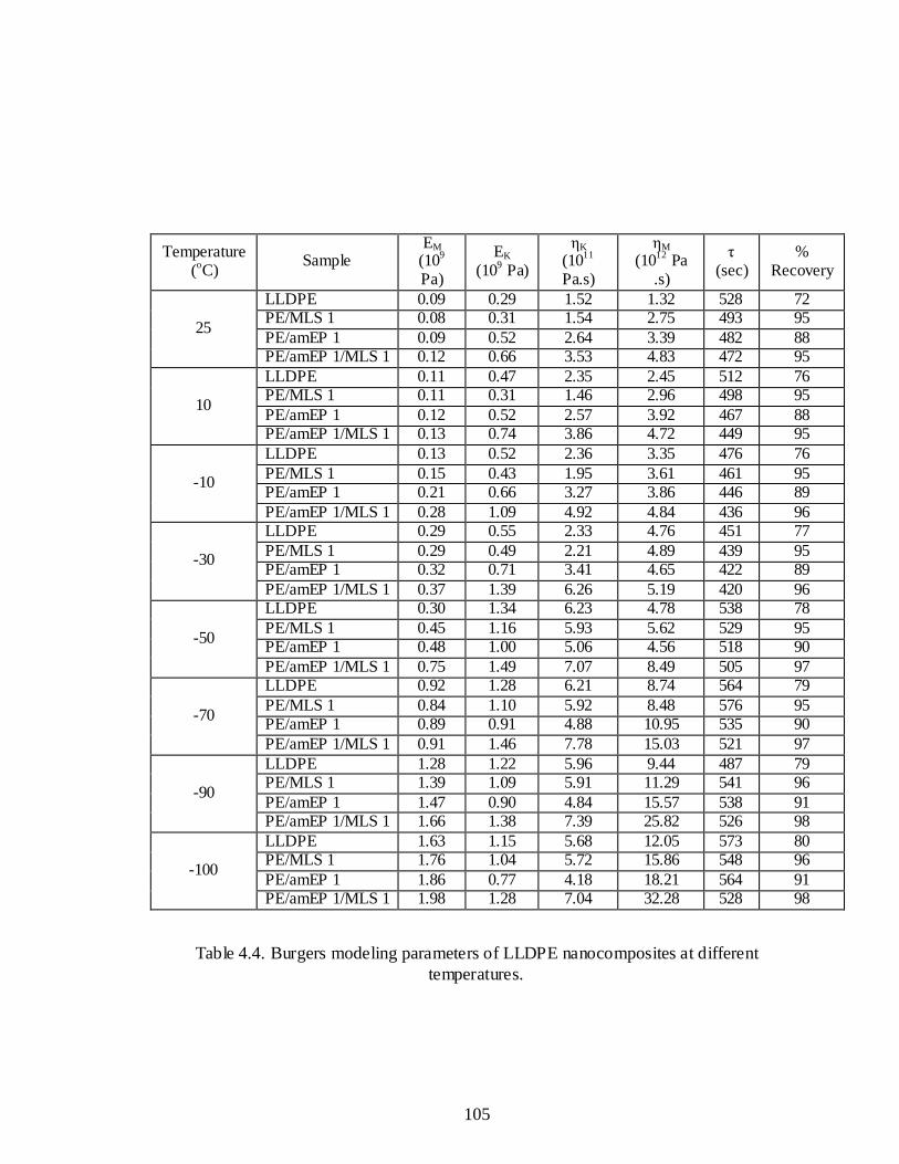
105
Temperature (
oC)
Sample EM
(109
Pa)
EK
(109 Pa)
ηK
(1011
Pa.s)
ηM (10
12 Pa
.s)
τ (sec)
% Recovery
25
LLDPE 0.09 0.29 1.52 1.32 528 72 PE/MLS 1 0.08 0.31 1.54 2.75 493 95
PE/amEP 1 0.09 0.52 2.64 3.39 482 88 PE/amEP 1/MLS 1 0.12 0.66 3.53 4.83 472 95
10
LLDPE 0.11 0.47 2.35 2.45 512 76 PE/MLS 1 0.11 0.31 1.46 2.96 498 95
PE/amEP 1 0.12 0.52 2.57 3.92 467 88 PE/amEP 1/MLS 1 0.13 0.74 3.86 4.72 449 95
-10
LLDPE 0.13 0.52 2.36 3.35 476 76
PE/MLS 1 0.15 0.43 1.95 3.61 461 95 PE/amEP 1 0.21 0.66 3.27 3.86 446 89
PE/amEP 1/MLS 1 0.28 1.09 4.92 4.84 436 96
-30
LLDPE 0.29 0.55 2.33 4.76 451 77
PE/MLS 1 0.29 0.49 2.21 4.89 439 95 PE/amEP 1 0.32 0.71 3.41 4.65 422 89
PE/amEP 1/MLS 1 0.37 1.39 6.26 5.19 420 96
-50
LLDPE 0.30 1.34 6.23 4.78 538 78
PE/MLS 1 0.45 1.16 5.93 5.62 529 95 PE/amEP 1 0.48 1.00 5.06 4.56 518 90
PE/amEP 1/MLS 1 0.75 1.49 7.07 8.49 505 97
-70
LLDPE 0.92 1.28 6.21 8.74 564 79
PE/MLS 1 0.84 1.10 5.92 8.48 576 95 PE/amEP 1 0.89 0.91 4.88 10.95 535 90
PE/amEP 1/MLS 1 0.91 1.46 7.78 15.03 521 97
-90
LLDPE 1.28 1.22 5.96 9.44 487 79 PE/MLS 1 1.39 1.09 5.91 11.29 541 96
PE/amEP 1 1.47 0.90 4.84 15.57 538 91 PE/amEP 1/MLS 1 1.66 1.38 7.39 25.82 526 98
-100
LLDPE 1.63 1.15 5.68 12.05 573 80 PE/MLS 1 1.76 1.04 5.72 15.86 548 96
PE/amEP 1 1.86 0.77 4.18 18.21 564 91 PE/amEP 1/MLS 1 1.98 1.28 7.04 32.28 528 98
Table 4.4. Burgers modeling parameters of LLDPE nanocomposites at different
temperatures.

106
4.3.3.2.1. Time-Independent Elasticity EM
The Burgers constitutive equation shows that the modulus EM of the Maxwell
spring determines the instantaneous elastic creep strain, which can be immediately
recovered on removal of stress. In general, the nanocomposites showed higher values of
EM than the neat matrix at each temperature. Among the nanocomposites, LLDPE/amEP
1/MLS 1 behaved with the highest elasticity. In the case of LLDPE/MLS systems, the
nanoclay layers could bear load because of the large aspect ratio of individual platelets
while discounted by the slippage of stacks and large amount of unexfoliated layers.
Hence, the resulting EM of LLDPE/amEP 1/MLS 1 was higher than that of the neat
matrix.
The variations of EM of the tested materials under various temperatures illustrated
the reinforcing characteristics of the nanofiller. The EM of each specimen showed an
increasing tendency with decreasing temperature, which could be explained by the fact
that the bulk materials became stiffer at lower temperatures and the stiffness was thus
increased with a higher instantaneous modulus as depicted by the tensile test results
(Table 4.3).

107
0
0.5
1
1.5
2
2.5
3
LLDPE PE/MLS 1 PE/amEP 1 PE/amEP 1/MLS 1
EM
(GP
a)
25 C 10 C -10 C -30 C -50 C -70 C -90 C -100 C
Figure 4.8. Temperature dependence of Burgers EM.
At 25 oC, the EM showed comparatively small changes between the neat PE
matrix and the nanocomposites, and the instantaneous elasticity was not altered much by
the addition of nanofiller. The instantaneous elasticity EM corresponded reasonably to the
elasticity of the crystalline part of the polymer, which took the immediate load because of
the high stiffness compared to the amorphous polymer. The crystallinity of each
specimen was not obviously altered with the addition of the MLS particles [14], which
implied that the load bearing parts between the neat matrix and the nanocomposites were
not greatly different.
As temperature was decreased to lower temperatures reaching -100 oC, EM of each
specimen increased. Among the observed specimens, the nanocomposites behaved with

108
much better elasticity than the pure matrix, showing an effective reinforcement by the
addition of nanofiller.
At -100 oC, EM increased from 1.63 GPa for the pure LLDPE to 1.98 for the
addition of 1% of amEP and MLS. These results depict the contribution of amEP and
MLS to the elasticity of the bulk material. Below the β-transition temperature, polymer
chains began to become less active. Consequently, the stiffness of bulk material
increased, which resulted in the higher value of EM compared to that at room temperature.
4.3.3.2.2. Retardant Elasticity EK and Viscosity ηK
The retardant elasticity EK and viscosity ηK of each specimen showed a similar
dependency as the instantaneous elasticity EM, increasing with decreasing temperature.
The deformation of the Kelvin unit of each material also decreased with the decreasing
temperature. The time-dependent EK and ηK in the Kelvin unit are associated with the
stiffness and viscous or oriented flow of amorphous polymer chains in the short term,
respectively.
EK and ηK of the nanocomposites increased considerably with decreasing
temperature, showing high-temperature dependency. The materials with relatively higher
bulk modulus deformed very little at lower temperatures, which showed that the Kelvin
unit behaved with higher modulus and lower viscous flow. With decreasing temperature,
the orientation movement of amorphous chains, including elastic deformation and
viscous flow, became difficult, resulting in the higher EK and ηK.
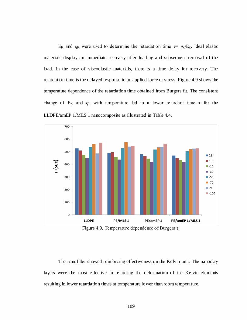
109
EK and ηK were used to determine the retardation time τ= ηK/EK. Ideal elastic
materials display an immediate recovery after loading and subsequent removal of the
load. In the case of viscoelastic materials, there is a time delay for recovery. The
retardation time is the delayed response to an applied force or stress. Figure 4.9 shows the
temperature dependence of the retardation time obtained from Burgers fit. The consistent
change of EK and ηK with temperature led to a lower retardant time τ for the
LLDPE/amEP 1/MLS 1 nanocomposite as illustrated in Table 4.4.
0
100
200
300
400
500
600
700
LLDPE PE/MLS 1 PE/amEP 1 PE/amEP 1/MLS 1
τ(s
ec)
25
10
-10
-30
-50
-70
-90
-100
Figure 4.9. Temperature dependence of Burgers τ.
The nanofiller showed reinforcing effectiveness on the Kelvin unit. The nanoclay
layers were the most effective in retarding the deformation of the Kelvin elements
resulting in lower retardation times at temperature lower than room temperature.
110
At temperatures below the β-transition temperature, the amorphous polymer becomes less
active. Thereafter, the polymer chains have restricted mobility. The Kelvin unit could not
be deformed further; therefore, a higher retardant time τ is observed.
4.3.3.2.3. Permanent Viscous Flow ηM
Following the discussion of the effect of the addition of amEP and MLS on the
instantaneous and time-dependent recoverable parameters in the Burgers constitutive
equation, it is of importance to provide an analysis of ηM which represents the
irrecoverable creep in a creep-recovery experiment. The effect of temperature on such
parameter is presented in Table 4.4.
From Table 4.4, it can be seen that ηM is strongly dependent on temperature. It can
be considered that ηM is associated with the damage from crystallized polymer or oriented
noncrystalline regions, such as the pulling out of chain folds by a crystal slip process and
the breaking of an intercrystalline tie molecule or the irreversible deformation from
amorphous regions, such as breaking of bridging segments between the clay particles and
the polymer chains.
At room temperature, ηM of the pure LLDPE increases with the addition of 1%
amEP and 1% MLS separately. The value of ηM increases from 1.32 for pure LLDPE to
4.83 with the addition of 1% amEP and 1% MLS as illustrated in Table 4. The results
show that no damage of the crystallized polymer occurred due to the fact that the stress
levels applied are still within the elastic limits of the crystallized part of the polymer. The
enhanced deformation resistance was obtained to the presence of amEP and MLS in the
111
LLDPE nanocomposite which acted to form a stiff structure together with the crystallized
molecules.
As temperature is decreased below the β-transition temperature, ηM significantly
increases. The irreversible deformation is diminished by the addition of amEP and MLS
to the LLDPE matrix, which enhanced the elasticity of the nanocomposites at lower
temperatures. The results are supported by the higher % recovery obtained with the
addition of amEP and MLS.
4.3.3.3. Viscoelastic Response
To compare the creep compliance obtained for the different compositions, creep
compliance curves were fitted with the KWW stretched exponential function,
])/exp(1[)( 0
tDtD
where D(t) is the creep compliance, τ is the characteristic retardation time, and β is a
creep shape parameter. The results of the curve fit parameters are tabulated in Table 4.5.
OriginLab® nonlinear least-squares data analysis software was used for the numerical
analysis of the creep compliance curve fits.

112
Temperature (oC) Sample τKWW βKWW
25
LLDPE 1.47 0.50
PE/MLS 1 0.89 0.21
PE/amEP 1 0.93 0.19
PE/amEP 1/MLS 1 0.86 0.21
10
LLDPE 0.75 0.26
PE/MLS 1 0.64 0.27
PE/amEP 1 0.82 0.22
PE/amEP 1/MLS 1 0.75 0.24
-10
LLDPE 0.64 0.31
PE/MLS 1 0.61 0.31
PE/amEP 1 0.68 0.27
PE/amEP 1/MLS 1 0.69 0.27
-30
LLDPE 0.53 0.33
PE/MLS 1 0.54 0.33
PE/amEP 1 0.69 0.27
PE/amEP 1/MLS 1 0.67 0.28
-50
LLDPE 0.68 0.28
PE/MLS 1 0.53 0.34
PE/amEP 1 0.72 0.27
PE/amEP 1/MLS 1 0.80 0.26
-70
LLDPE 0.70 0.32
PE/MLS 1 0.60 0.29
PE/amEP 1 0.86 0.23
PE/amEP 1/MLS 1 0.91 0.23
-90
LLDPE 0.66 0.26
PE/MLS 1 0.64 0.24
PE/amEP 1 0.90 0.22
PE/amEP 1/MLS 1 0.95 0.22
-100
LLDPE 0.68 0.21
PE/MLS 1 0.66 0.21
PE/amEP 1 0.92 0.20
PE/amEP 1/MLS 1 0.99 0.21
Table 4.5. KWW fit parameters of LLDPE nanocomposites at different temperatures.

113
Figures 4.10 and 4.11 compare the KWW fit parameters of LLDPE
nanocomposites at different temperatures. A retardation time represents resistance offered
by the microstructure to the elastic deformation of the system. As retardation time
decreases (less resistance occurs), system response becomes more elastic.
0
0.2
0.4
0.6
0.8
1
1.2
1.4
1.6
LLDPE PE/MLS 1 PE/amEP 1 PE/amEP 1/MLS 1
τ KW
W (
se
c)
25 C 10 C -10 C -30 C -50 C -70 C -90 C -100 C
Figure 4.10. Temperature dependence of retardation time values obtained from the KWW fit.

114
0
0.1
0.2
0.3
0.4
0.5
0.6
LLDPE PE/MLS 1 PE/amEP 1 PE/amEP 1/MLS 1
βK
WW
25 C 10 C -10 C -30 C -50 C -70 C -90 C -100 C
Figure 4.11. Temperature dependence of β values obtained from the KWW fit.
The general trend observed in the retardation time for the LLDPE nanocomposites
can be summarized as follows: Retardation time decreases linearly with decreasing
temperature above the β-transition temperature. Below the β-transition temperature,
retardation time increases linearly with decreasing temperature. This behavio r is
exhibited because below the β-transition temperature, the material is in its glassy state
where molecular mobility is hindered, reducing the polymer elasticity.
Comparing the retardation time among the different LLDPE compositions, we
observed that the addition of MLS reduced the retardation time as compared to the neat
PE. This reduction can be attributed to the addition of the rigid MLS platelets, which
increases the matrix elasticity. Addition of amEP into the LLDPE matrix further
increased retardation time. This increase can be related to the amorphous nature of the
115
compatibilizer. A combination of amEP and MLS seemed to reduce the retardation time
above the β-transition temperature and to increase it below the β-transition temperature.
Figure 4.11 shows the variation of β at different temperatures of LLDPE
nanocomposites. Considering pure LLDPE, as temperature decreases, β values increase,
indicating a broader distribution of retardation times. β reaches a maximum at -30 oC (β-
transition temperature). Below -30 oC, β decreases linearly with decreasing temperature.
The same trend is observed with the addition of amEP and MLS separately and
combined with the LLDPE matrix. The values of β do not show a significant change with
the addition of 1% MLS. Addition of 1% amEP reduces the β values; the values remain
unchanged with the addition of 1% of amEP and 1% MLS. According to the coupling
theory proposed by Ngai et al. [16], a decrease in the β parameter can be interpreted as a
strengthening of the coupling between the relaxing species and the medium and is related
to an overall decrease of the molecular mobility. It is known that the crystalline phase
hinders the molecular mobility of the amorphous one [17]. A decrease of β measured by a
differential scanning calorimeter (from 0.4 to 0.2) was detected for amorphous and semi-
crystalline polyethylene terephthalate (PET), respectively [18].

116
4.4. Conclusions
The creep behavior of LLDPE nanocomposites at different temperatures was
analyzed. Creep compliance decreased with the addition of MLS particles. This effect
was related to the enhancement of the tensile properties. The reduction in creep
compliance with the addition of the clay leads to a material with higher dimensional
stability; the materials behaved with higher stiffness and lower deformability under long-
term loading situations because of the addition of inorganic nanofiller.
For the Burgers model, the instantaneous modulus EM, the retardant modulus EK,
and viscosity ηK showed an explicit dependence on temperature. They also increased with
the addition of clay. EM showed an increase with decreasing temperature, which was also
reflected in an increase of the yield stress and modulus of the materials with decreasing
temperature.
Above the beta transition temperature, a decrease in the retardation time and an
increase in the β values were observed with decreasing temperature. Below this
temperature, the trends were reversed. This behavior was explained by the hindered
mobility of the amorphous region.
4.5. References
1. K.K. Maniar., Polymer-Plastics Tech. and Eng., 43, 427-443 (2004).
2. D. Martin, P. Halley, R. Truss, M. Murphy, O. Jackson, and O.Y. Kwon, Polym.,
1774-1779(2003).

117
3. G. Liang, J. Xu, S. Bao, and W. Xu, J. Appl. Polym. Sci., 91, 3974-3980 (2004).
4. G. Malucelli, S. Ronchetti, N. Lak, A. Priola, N.T. Dintcheva, and F.P. La Manta, Eur.
Polym. J., 43, 328-335 (2007).
5. J.J. Aklonis and W.J. MacKnight. Introduction to Polymer Viscoelasticity, John Wiley
& Sons: New York (1983).
6. C.J. Perez, V.A. Alvarez, and A. Vasquez, Mat. Sci. and Eng. A, 480, 259-265 (2008).
7. J.L. Yang, Z. Zhang, A. Schlarb, and K. Friedrich, Polym, 47, 6745-6758 (2006).
8.A. Ranade, K. Nayak, D. Fairbrother, and N.A. D’Souza, Polym, 46, 7323-7333 (2005).
9. A.D. Nunez, N.E. Marcovich, and M.I. Aranguren, Polym. Sci. and Eng., 44, 1594-
1603 (2004).
10. C. Marais and G. Villoutreix, J. Appl. Polym. Sci., 69, 1983-1991 (1998).
11. M.D. Alvarez, W. Canet, F. Cuesta, and M. Lamua, Z Lebensm Unters Forsch A, 207,
356-362 (1998).
12. J. Beckmann and G.B. McKenna, Polym. Eng. and Sci., 37, 1459-1468 (1997).
13. J.M. Cheriere, L. Belec, and J.L. Gacougnolle, Polym. Eng. and Sci., 37, 1664-1671
(1997).
14. A. Shaito, D. Fairbrother, J. Sterling, N.A D’Souza, “Nonlinear creep deformation in
PE nanocomposites: effect of amorphous maleated PE compatibilizers on room
temperature creep”, Polym. Eng. and Sci, submitted (2008).
15. M. Niaounakis and E. Kontou, J. Polym. Sci.: Part B: Polym. Phys., 43, 1712-1727
(2005).
16. K.L. Ngai, A.K. Rajagopal, and S. Teitler, J. Chem. Phys., 88, 5086 (1988).
17. N.G. McCrum, B.E. Read, and G. Williams, Anelastic and Dielectric Effects in
Polymeric Solids, Dover, New York, (1991).
18. N.M. Alves, J.F. Mano, E. Balaguer, J.M. Meseguer Duenas, and J.L. Gomez
Ribelles, Polym. , 43, 4111-4122 (2002).

118
CHAPTER 5
EFFECT OF STRESS ON ROOM TEMPERATURE MOLECULAR RELAXATION
5.1. Introduction
Polymer nanocomposites (PNs) have generated significant interest in science and
engineering over the past years [1-4]. The time independent mechanical properties of
polymer nanocomposites have been well investigated [5-6]. In most practical
applications, isothermal compliance of the polymeric material not only depends on stress
but also on time, and hence the time-dependent response i.e. , creep behavior is of
significant importance [7].
The theoretical background of creep behavior in solid polymers is well studied
within the range of linear viscoelasticity [8]. In this region, the creep compliance is
assumed to be a function of time only, and not of stress and strain. Beyond a certain
strain limit, the isothermal creep compliance becomes a function of time and stress (or
strain). This non- linear viscoelastic behavior plays an important role in most applications
[9]. Liu et al. [10] studied the nonlinear viscoelastic creep of polyethylene (PE). They
found the material response to be dependent on stress. The nonlinear time dependent
response of the material was modeled using multiple Kelvin elements. The validation of
the model is done by comparison with tensile test result. Yang et al. [11] modeled the
long term performance of polyamide 66 nanocomposites using Burgers viscoelastic creep
model. The variations in the simulating parameters were used to study the variation of the

119
material properties with stress. The predicting results showed the enhancement in the
creep resistance even at extended long time scale.
Several mechanical models have been used to explain the creep, recovery, and
stress relaxation aspects of polymeric materials of which the spring-dashpot model;
Maxwell-Voigt model and Burger model, and models based on distribution functions like
the Kohlrausch-Williams-Watts (KWW) function are commonly used. The KWW
function, which is an empirically stretched exponential function, is mainly used to
explain the time-dependent behavior of amorphous materials [12]. In this paper, the
structure-property relationship is carried out by the parameters analysis of the Burgers
model at different stress levels to account for the nonlinear behavior. The variations of
these parameters illustrate the influence of the fillers on the creep resistance of the bulk
LLDPE matrix. Also, the breadth of relaxation is considered by analyzing the fit
parameters of the KWW exponential stretched function.
5.2. Experimental
5.2.1. Materials
LLDPE DOWLEX 2056G (Dow chemical company) was used to prepare the PE
nanocomposite films (density = 0.92 g/cc; Melt index = 1.0 gm/10 min).
Montmorillonite- layered silicate (MLS) (Cloisite 15A™), supplied by southern clay
products, was used as the nanofiller. An amorphous maleic anhydride functionalized
elastomeric copolymer, Exxelor VA 1803 (ExxonMobil corporation), was used as a
compatibilizer between the MLS and the PE matrix. Exxelor VA 1803 has a nominal

120
density of 0.86 g/cm3 and a melt index of 3 g/10 min (ASTM D1238, 230 oC, 2.16 kg).
The maleic anhydride (MA) level is in the range of 0.5 to 1%.
5.2.2. Sample Preparation
Nanocomposites were compounded with a Haake TW100 twin-screw extruder
with a temperature profile of 200, 200, 205, and 210 oC for zones 1 to 4, respectively. PE
films 1.5 mil (0.04 mm) thick were processed with a Killion single-screw extruder (L/D =
24:1), fitted with a dual- lip air ring and a die diameter of 2 inches. Blends of
PE+amEP+MLS were made, and the mixtures were compounded and pelletized. The
compounded pellets were then processed into a blown film. Table 5.1 summarizes the
concentrations used.
Sample LLDPE (wt %)
Exxelor VA 1803 (wt %)
MLS (wt %)
LLDPE 100 0 0
PE/MLS 1 99 0 1
PE/amEP 1 99 1 0
PE/amEP 1/MLS 1 98 1 1
Table 5.1. Summary of concentrations used.
5.2.3. Tensile Testing
Yield stress and elastic modulus E were determined by using RSA III films
fixture with an extension rate of 0.208 mm/min.

121
5.2.4. Creep Testing
Uniaxial tensile creep tests were performed by using RSA III with the films
attachment. The desired constant stress to be applied for each measurement was
calculated to be 10, 25, and 50% of the yield stress. The constant stress was applied for 1
hour of loading followed by 1 hour of unloading. A linear displacement transducer with a
force capacity of 35 N was used to monitor the strain during the experiment. The creep
compliance was calculated by the ratio of the measured creep strain to the initial applied
stress.
5.3. Results and Discussion
5.3.1. Stress Dependence of Creep-Recovery Response
The experimental data of creep of LLDPE nanocomposites at various stress levels
is shown in Figure 5.1, where the creep compliance D (t) is defined as the ratio of the
measured time-dependent strain, ε (t), to the applied stress σ.
0
0.07
0.1
0.2
0 1000 2000 3000 4000 5000 6000 7000 8000
25 %
10 %
50 %
Cre
ep
Co
mp
lia
nc
e (
GP
a-1
)
Time (sec)
(a)

122
0
0.07
0.1
0.2
0 1000 2000 3000 4000 5000 6000 7000 8000
50 %
10 %
25 %C
reep
Co
mp
lian
ce (
GP
a-1
)
Time (sec)
(b)
0
0.04
0.08
0.1
0 1000 2000 3000 4000 5000 6000 7000 8000
10 %
50 %
25 %
Cre
ep
Co
mp
lian
ce (
GP
a-1
)
Time (sec)
(c)

123
0
0.08
0.2
0.3
0 1000 2000 3000 4000 5000 6000 7000 8000
10 %
25 %
50 %C
re
ep
Co
mp
lia
nc
e (
GP
a-1
)
Time (sec)
(d)
Figure 5.1. Creep compliance versus time plot of LLDPE nanocomposites: (a) pure LLDPE, (b) PE/1% MLS, (c) PE/1% amEP, (d) PE/1% amEP/1% MLS at room
temperature.
Figure 5.1 shows that creep compliance is stress-dependent at all stress levels and
that the creep compliance curve increases with the applied stress. This indicates that
LLDPE exhibits a strong nonlinear behavior with the stress dependence and time
dependence of creep compliance coupled. For most amorphous polymers, a linear
viscoelasticity and a transition from linear to non- linear viscoelasticity exist. However,
no linearity for LLDPE was observed as seen in Figure 5.1. The linearity of the materials
seems to exist at relatively small stresses, possibly due to the structural features of the
semicrystalline polymer.
5.3.2. Burgers Modeling Parameters
To evaluate the changes of the material properties with the addition of amEP and
MLS, Burgers model was used to fit the creep data of LLDPE nanocomposites at the
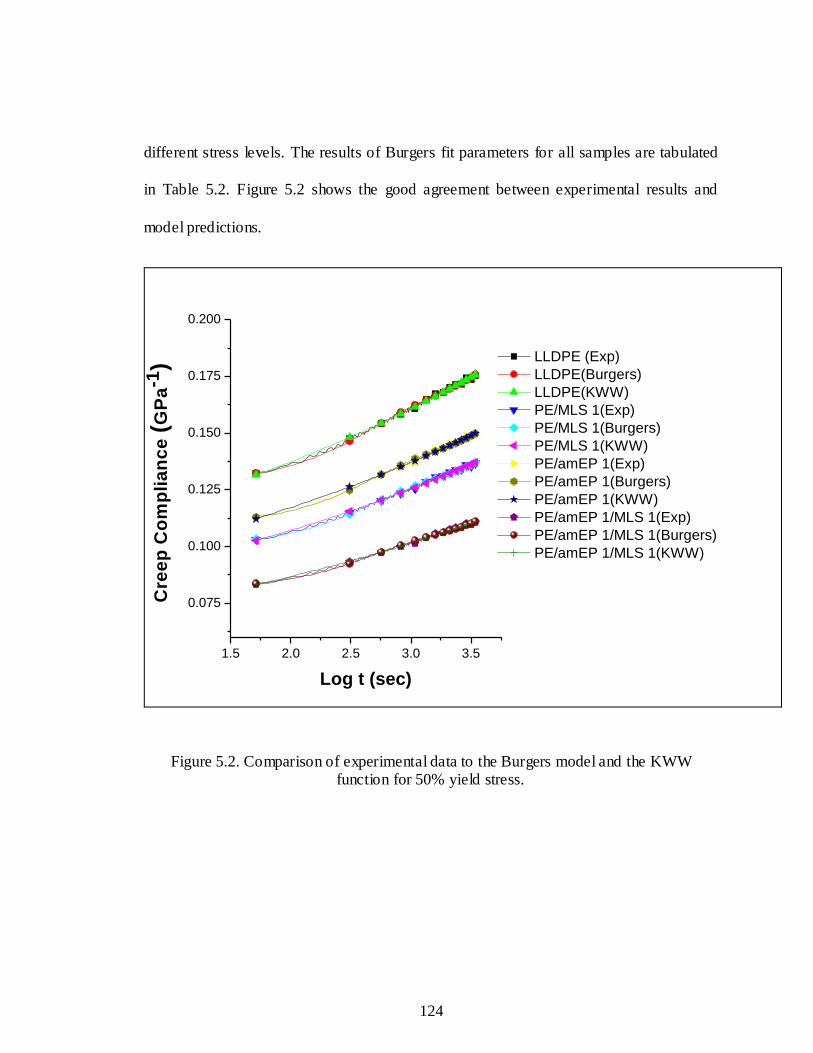
124
different stress levels. The results of Burgers fit parameters for all samples are tabulated
in Table 5.2. Figure 5.2 shows the good agreement between experimental results and
model predictions.
1.5 2.0 2.5 3.0 3.5
0.075
0.100
0.125
0.150
0.175
0.200
LLDPE (Exp)
LLDPE(Burgers)
LLDPE(KWW)
PE/MLS 1(Exp)
PE/MLS 1(Burgers)
PE/MLS 1(KWW)
PE/amEP 1(Exp)
PE/amEP 1(Burgers)
PE/amEP 1(KWW)
PE/amEP 1/MLS 1(Exp)
PE/amEP 1/MLS 1(Burgers)
PE/amEP 1/MLS 1(KWW)
Cre
ep
Co
mp
lia
nc
e (
GP
a-1
)
Log t (sec)
Figure 5.2. Comparison of experimental data to the Burgers model and the KWW function for 50% yield stress.

125
Sample Applied Stress
(% yield stress)
EM
(109 Pa)
EK
(109 Pa)
ηK
(1011 Pa.s)
ηM
(1012 Pa .s)
τ
(sec)
LLDPE
10 0.08 3.02 2.10 5.24 490
25 0.09 1.58 2.15 2.51 510
50 0.09 0.29 1.52 1.32 528
PE/MLS 1
10 0.06 3.27 1.07 5.62 475
25 0.08 1.29 1.45 2.27 486
50 0.08 0.31 1.54 2.75 493
PE/amEP 1
10 0.10 3.85 2.57 6.04 459
25 0.10 1.67 2.41 2.82 473
50 0.09 0.52 2.64 3.39 482
PE/amEP 1/MLS 1
10 0.11 4.47 3.91 7.00 445
25 0.12 1.71 4.01 3.36 466
50 0.12 0.66 3.53 4.83 472
Table 5.2. Burgers fit parameters of LLDPE nanocomposites.
The modulus EM of the Maxwell spring determines the instantaneous elastic creep
strain, which could be immediately recovered on the removal of stress. The addition of
1% MLS did not show significant changes at all stress levels as compared to the neat PE
matrix. Adding 1% amEP into LLDPE showed marginal changes. However
LLDPE/amEP 1/MLS 1 showed 38% and 33% at 10 and 25% yield stress levels
respectively. In the case of LLDPE/MLS systems, the nanoclay layers could bear load
because of the large aspect ratio of the individual platelet while discounted by the
slippage of stacks and large amount of unexfoliated layers. Hence, the resulting EM of
LLDPE/amEP 1/MLS 1 was higher than the neat matrix. This increase reflects the tensile
test results in which the nanocomposites with amEP and MLS had higher yield stress and
modulus. The increasing values of EM with the applied stress provided the fact that the

126
elasticity of the nanocomposites was not altered with the addition of amEP and MLS to
the LLDPE matrix.
The time-dependent parameters EK and ηK were considerably decreased with
increasing stress, showing high stress dependency. This indicated the fact that materials
with a relatively higher bulk modulus deformed very little, and the Kelvin unit behaved
with a higher modulus and very difficult viscous flow. With increasing stress, the
orientation movement of the amorphous chains including elastic deformation and viscous
flow became difficult resulting in lower EK and ηK.
EK and ηK were used to determine the retardation time τ= ηK/EK. Ideal elastic
materials display an immediate recovery after loading and subsequent removal of the
load. In the case of viscoelastic materials, there is a time delay for recovery. The
retardation time is the delayed response to an applied force or stress. Figure 5.3 shows the
stress dependence of the retardation time obtained from Burgers fit. The consistent
change of EK and ηK with stress led to a lower retardant time τ for the LLDPE/amEP
1/MLS 1 nanocomposite as illustrated in Table 5.2. The increase observed in retardation
time with the applied stress for all samples can be explained by the orientational
hardening of the polymer chains including plastic deformation and viscous flow of the
crystalline and amorphous chains. The nanofiller showed reinforcing effectiveness on the
Kelvin unit. The nanoclay layers were most effective in retarding the deformation of the
Kelvin elements resulting in lower retardation times for the LLDPE nanocomposite.
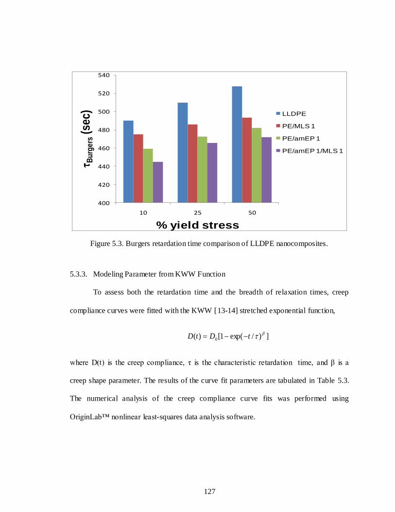
127
400
420
440
460
480
500
520
540
10 25 50
τ Bu
rge
rs(s
ec)
% yield stress
LLDPE
PE/MLS 1
PE/amEP 1
PE/amEP 1/MLS 1
Figure 5.3. Burgers retardation time comparison of LLDPE nanocomposites.
5.3.3. Modeling Parameter from KWW Function
To assess both the retardation time and the breadth of relaxation times, creep
compliance curves were fitted with the KWW [13-14] stretched exponential function,
])/exp(1[)( 0
tDtD
where D(t) is the creep compliance, τ is the characteristic retardation time, and β is a
creep shape parameter. The results of the curve fit parameters are tabulated in Table 5.3.
The numerical analysis of the creep compliance curve fits was performed using
OriginLab™ nonlinear least-squares data analysis software.

128
Sample Applied Stress
(% yield stress) τKWW (sec) βKWW
LLDPE
10 0.89 0.21
25 0.93 0.19
50 0.95 0.21
PE/MLS1
10 0.89 0.19
25 0.91 0.21
50 0.95 0.19
PE/amEP 1
10 0.88 0.20
25 0.90 0.19
50 0.92 0.20
PE/amEP/MLS1
10 0.85 0.21
25 0.89 0.20
50 0.92 0.20
Table 5.3. KWW curve fitting parameters.
Figures 5.4 and 5.5 compare the KWW fit parameters of LLDPE nanocomposites.
A retardation time represents resistance offered by the microstructure to the elastic
deformation of the system. As the retardation time decreases (i.e., as less resistance
occurs), the system response becomes more elastic. The results of the samples
investigated are tabulated in Table 4.

129
0.78
0.80
0.82
0.84
0.86
0.88
0.90
0.92
0.94
0.96
1 0 2 5 5 0
τ KW
W (s
ec)
% yield stress
LLDPE
PE/MLS1
PE/amEP 1
PE/amEP 1/MLS1
Figure 5.4. KWW retardation time comparison of LLDPE nanocomposites.
0.00
0.05
0.10
0.15
0.20
0.25
0.30
1 0 2 5 5 0
βK
WW
% yield stress
LLDPE
PE/MLS1
PE/amEP 1
PE/amEP 1/MLS1
Figure 5.5. Comparison of βkww for the different LLDPE nanocomposites.

130
In the analysis of the parameters, stress effects and materials effects are to be
considered. At a stress of 10 % yield stress, the addition of 1% MLS decreases the
retardation time. The results can be explained by the addition of the rigid MLS particles,
which act to increase the elasticity of the matrix and hence reduce the retardation time.
The corresponding effect on the breadth of relaxation, which is inversely related
to β, is to increase it substantially. A minimum in the values of retardation time is
obtained when a combination of 1% MLS and 1% amEP is used The values of β
remained constant (β = 0.20 ± 0.01) despite the different amounts of MLS and amEP that
have been added into the PE matrix.. The results obtained for LLDPE nanocomposites
suggest that a combination of 1%MLS and 1% amEP gives the lowest retardation time. A
similar behavior is observed at 25 and 50 % yield stress.
5.4. Conclusion
The modeling of the creep response of LLDPE nanocomposites was successfully
conducted by using Burgers model and KWW stretched exponential function. The
simulating parameters helped to comprehensively understand the improvement of the
creep resistance by the addition of amEP and MLS and suggested the structure-property
relationship representatively.
From Burgers model, the instantaneous modulus EM showed an explicit
dependence on stress which indicated that the materials behaved with higher stiffness and
lower deformability under long-term loading. The addition of amEP and MLS
contributed to the lower retardation time and thus resulted in reduced creep deformation.
131
The results of retardation time from KWW function at all stress levels matched Burgers
prediction for the different materials.
5.5 References
1.K.K. Maniar., Polymer-Plastics Tech. and Eng., 43, 427 (2004).
2.D. Martin, P. Halley, R. Truss, M. Murphy, O. Jackson, and O.Y. Kwon, Polym., 1774
(2003).
3.G. Liang, J. Xu, S. Bao, and W. Xu, J. Appl. Polym. Sci., 91, 3974 (2004)
4.G. Malucelli, S. Ronchetti, N. Lak, A. Priola, N.T. Dintcheva, and F.P. La Manta, Eur.
Polym. J., 43,
328 (2007).
5.S.C. Tjong, J. Matr. Sci. Eng., 53, 73 (2006).
6.J.N. Coleman, U. Khan, K. Friedrich, W.J. Blau, Y.K. Gun’ko, Carbon, 44, 1624
(2006).
7.J. Raghavan, M. Meshii, Compos. Sci. Technol., 57, 1673 (1997).
8.J.J. Aklonis and W.J. MacKnight. Introduction to Polymer Viscoelasticity, John Wiley
& Sons: New York (1983).
9.J. Kolarik, A. Pergoretti, Polym. , 47, 346 (2006).
10.H Liu, MA Polak, 33rd Annual General conference of the Canadian Society for Civil
Engineering 2005.
11.J.L. Yang, Z. Zhang, A. Schlarb, and K. Friedrich, Polym., 47, 6745-6758 (2006).
12.K.S. Fancey, J. Mater. Sci., 40, 4827 (2005).
13. F. Kohlrausch, Pogg. Ann Physics, 12, 393 (1847).
14.G. Williams, D.C. Watts, Trans Faraday Soc, 66, 80 (1970).

132
CHAPTER 6
SEPARATION OF STRUCTURAL TIME DEPENDENT DEFORMATION DUE TO
STRESS MAGNITUDE
6.1 Introduction
Viscoelastic behavior exhibits various properties. Creep under constant stress,
stress relaxation under constant strain, time-dependent recovery of strain after constant
load is removed, time-dependent creep rupture, and frequency dependence of fatigue
strength are a few examples. If a material does not recover completely after the removal
of the constant load in a creep test and if an unrecoverable strain persists, the material is
said to have a residual viscoplastic strain. Nonlinearities may be due to intrinsic behavior,
local nonlinear stress-strain behavior, or macro-stress-strain equations that are large to be
modeled with local continuum mechanics models. Although linear viscoelastic principles
are useful for describing the long-term properties, they are not adequate when the stresses
are so high that non- linearity is observed in the response of the material.
Recent studies have focused on polymer nanocomposites as novel materials [1].
The mechanical properties of polymer nanocomposites have been extensively studied;
and enhanced performances, such as strength, stiffness, and toughness, have been
achieved to extend the different applications such as load-carrying components [2].
Important factors such as filler concentration, dispersion state, and interfacial bonding are
considered to be able to significantly influence the properties of bulk materials. Because
of their nanoscale size and the huge interfacial area of the nanoparticles, a low
133
concentration of these nanoparticles is usually used. Many researchers have reported that
the incorporation of these nanoparticles can cause a significant improvement in
mechanical and thermal properties. Even though their strength and elastic properties have
been studied in recent years [3-6], data on the time-dependent behavior of these materials
is still lacking. Consequently, studies on creep of these new promising nanocomposites
are very important and necessary. Pegoretti et al. [7] studied the creep resistance of
polyethylene terephthlate (PET)/MLS nanocomposites. A decrease in creep compliance
was observed in the nanocomposites when compared to the neat matrix. Vlasve ld et al.
[8] also studied the effects of physical aging and moisture on the creep performance of
polyamide 6 (PA6) filled with layered silicates. Creep compliance was found to be
reduced by the addition of the layered silicates.
A previous work by our laboratory focused on the improvement of the creep
resistance of LLDPE/MLS nanocomposites for potential use in s tratospheric balloons [3].
Stratospheric balloons are large aerospace structures with the primary bearing material
being linear low-density polyethylene (LLDPE) that is 10 to 20 µm in thickness. The
viscoelastic behavior of these structures has been studied extensively [9-11]. Of particular
importance is the analysis of the state of stress in such structures. Several studies showed
the good ability of Schapery model to predict the stress response in a broad class of
materials. Papanicolaou et al. [12] studied the non- linear viscoelastic response of
unidirectional carbon-fiber-reinforced polymer matrix. Creep and recovery measurements
in tension with different stress levels were made for this purpose. A modified Schapery
model was used to describe the non- linear viscoelastic response and determination of

134
non- linear parameters. A viscoplastic term was added for the description of the total
strain response in the system. The viscoplastic strain was revealed as a remaining strain at
the end of recovery. Good agreement between experimental data and theoretical results
was obtained. Papanicolaou et al. [13] further developed the technique suggested by
Zaoutsos [12] by means of an analytical prediction of nonlinearity parameters as a
function of the applied stress. The prediction takes into account certain characteristic
properties, such as linear and nonlinear stress threshold and the ultimate tensile strength
of the material. The validity of the model is confirmed by creep-recovery tests on a 90o
unidirectional carbon-fiber/epoxy-matrix composite. A decrease in the values of go with
respect to the applied stress level was mostly due to the hardening of the specific
material. The values of both g1 and g2 increased with increasing applied stress. Touatl et
al. [14] proposed a method to predict non- linear relaxation behavior from creep
experiments. For a given nonlinear creep properties and creep compliance, the Schapery
creep model could be transformed into a set of first-order nonlinear equations. The
solution of these equations enables obtaining the nonlinear stress relaxation curves. The
method was demonstrated on test data for polyurethane and showed good agreement with
the experimental results. Luna et al. [15] studied the nonlinear behavior of polypropylene
(PP) nanocomposites. The Schapery model was used to determine the overall
mastercurve from the behavior of the material at different load levels.
The material showed nonlinear behavior below the yield point and referred that to a
change in the structure of the material. Lai and Bakker [16] modeled the time-dependent
behavior of high-density polyethylene (HDPE) with a one-dimensional integral

135
representation. The total strain in the material could be decomposed into a recoverable
viscoelastic strain and an irrecoverable plastic strain. The viscoelastic deformat ion is
represented by the Schapery creep model. Rand et al. [11] studied the nonlinear behavior
of LLDPE. Stress-time-temperature superposition principles similar to time-temperature
superposition principles were used to form a “mastercurve.”
It is thus very common to account for the linear viscoelastic behavior of some
polymers when analyzing their short- and long-term performance. The assumption of
linearity is often used, even when the nonlinearity is significant because the nonlinearities
are not well understood and/or useful experimental and theoretical data are not available
for nonlinear characterization and analysis. The rapid growth of computing power and the
availability of advanced finite element software that allows for the use of customized
material models account for the computational aspects. The experimental characterization
of the mechanical aspects of the material remains a need. In this chapter, experimental
data are collected for LLDPE nanocomposites, and the results are used to study the
nonlinearities in the behavior of the material. Schapery’s nonlinear model is used to
describe the nonlinear effects.
6.2 Experimental
6.2.1 Sample Preparation
Nanocomposites were compounded by using a Haake TW100 twin-screw
extruder with a temperature profile of 200, 200, 205, and 210 oC for zones 1 to 4,
respectively. PE films 1.5 mil (0.04 mm) thick were processed with a Killion single-
screw extruder (L/D = 24:1), fitted with a dual- lip air ring and a die diameter of 2 inches.

136
Blends of PE + amEP+ MLS were made and the mixtures were compounded and
pelletized. The compounded pellets were then extruded into blown films. Table 6.1
summarizes the concentrations used.
Sample LLDPE (wt %)
Exxelor VA 1803 (wt %)
MLS (wt %)
LLDPE 100 0 0
PE/MLS 1 99 0 1
PE/amEP1 99 1 0
PE/amEP1/MLS 1 98 1 1
Table 6.1. Summary of composition used.
6.2.2 Tensile Testing
Yield stress, ultimate tensile strength (UTS), and elastic modulus E were
determined by using RSA III film fixture with an extension rate of 0.208 mm/min.
6.2.3 Creep Testing
Uniaxial tensile creep tests were performed by using RSA III with the films
attachment. The desired constant stress to be applied for each measurement was
calculated to be 10, 25, and 50% of the yield stress. The constant stress was applied for 1
hour of loading followed by 1 hour of unloading. A linear displacement transducer with a
force capacity of 35 N was used to monitor the strain during the experiment. The creep
compliance was calculated by the ratio of the measured creep strain to the initial applied
stress.
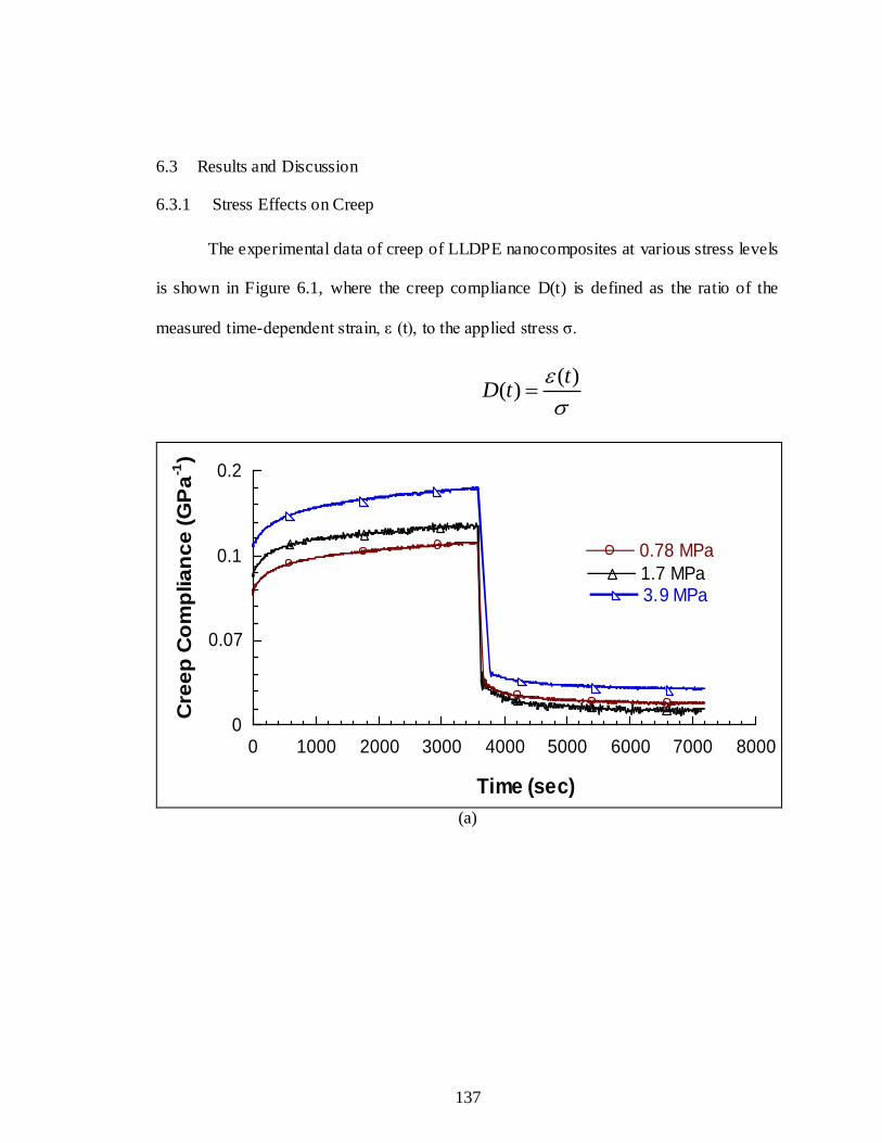
137
6.3 Results and Discussion
6.3.1 Stress Effects on Creep
The experimental data of creep of LLDPE nanocomposites at various stress levels
is shown in Figure 6.1, where the creep compliance D(t) is defined as the ratio of the
measured time-dependent strain, ε (t), to the applied stress σ.
)()(
ttD
0
0.07
0.1
0.2
0 1000 2000 3000 4000 5000 6000 7000 8000
1.7 MPa
0.78 MPa
3.9 MPa
Cre
ep
Co
mp
lia
nc
e (
GP
a-1
)
Time (sec)
(a)
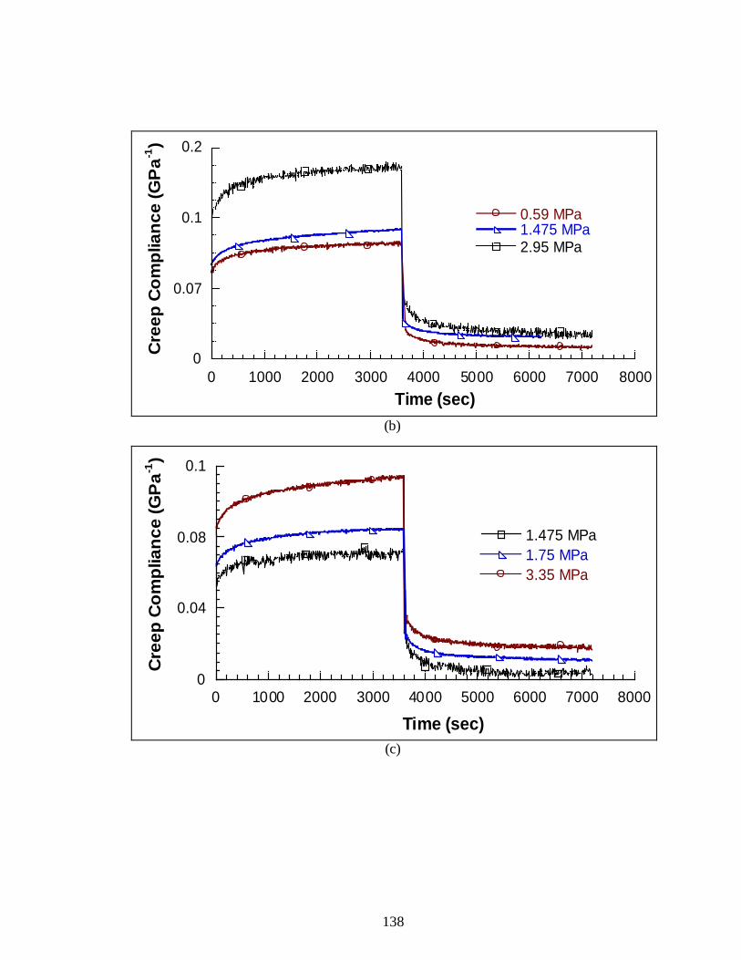
138
0
0.07
0.1
0.2
0 1000 2000 3000 4000 5000 6000 7000 8000
2.95 MPa
0.59 MPa1.475 MPa
Cre
ep
Co
mp
lia
nc
e (
GP
a-1
)
Time (sec)
(b)
0
0.04
0.08
0.1
0 1000 2000 3000 4000 5000 6000 7000 8000
1.475 MPa
3.35 MPa
1.75 MPa
Cre
ep
Co
mp
lia
nc
e (
GP
a-1
)
Time (sec)
(c)
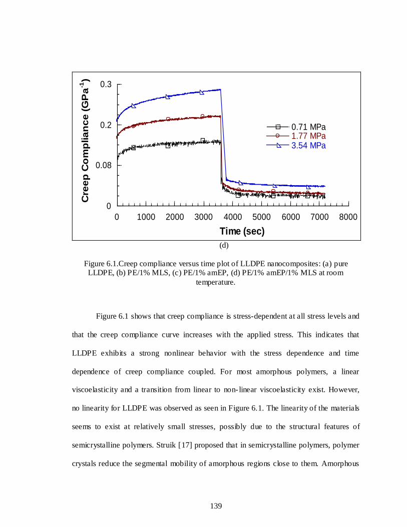
139
0
0.08
0.2
0.3
0 1000 2000 3000 4000 5000 6000 7000 8000
0.71 MPa1.77 MPa 3.54 MPa
Cre
ep
Co
mp
lia
nc
e (
GP
a-1
)
Time (sec)
(d)
Figure 6.1.Creep compliance versus time plot of LLDPE nanocomposites: (a) pure LLDPE, (b) PE/1% MLS, (c) PE/1% amEP, (d) PE/1% amEP/1% MLS at room
temperature.
Figure 6.1 shows that creep compliance is stress-dependent at all stress levels and
that the creep compliance curve increases with the applied stress. This indicates that
LLDPE exhibits a strong nonlinear behavior with the stress dependence and time
dependence of creep compliance coupled. For most amorphous polymers, a linear
viscoelasticity and a transition from linear to non- linear viscoelasticity exist. However,
no linearity for LLDPE was observed as seen in Figure 6.1. The linearity of the materials
seems to exist at relatively small stresses, possibly due to the structural features of
semicrystalline polymers. Struik [17] proposed that in semicrystalline polymers, polymer
crystals reduce the segmental mobility of amorphous regions close to them. Amorphous

140
regions far from these crystals remain undisturbed and hence are more mobile. For PE,
above its glass transition temperature, the amorphous regions far from the crystals are in
their rubbery state, whereas those near the crystals are still in their glassy state and hence
behave elastically. The amorphous region far from the crystals exhibits a non-linear
behavior induced by the applied stress accompanied by a change in the free volume
typical of amorphous polymers above their glass transition temperature.
The strong nonlinearity exhibited by LLDPE nanocomposites and the increase of
the creep compliance with the applied stress suggests the applicability of the time-stress
superposition principle. According to this principle, if the creep compliance curves are
plotted in logarithmic scale, then different curves at different stress levels can be
superposed by a horizontal shift. For thermorheologically complex materials such as
semicrystalline material, a vertical shift factor of the data plots along the y-axis should be
considered [18]. The concept of the vertical shift factor has been used by many authors
[19-21]. Although the real cause of the vertical shift is not clear, it is thought that it is a
representation of the change in crystallinity [22].
To obtain the mastercurve of the creep compliance curve, the reference stress σ0 is
chosen to be the lowest stress applied. The corresponding mastercurves of LLDPE
nanocomposites are shown in Figure 6.2.

141
Figure 6.2. Mastercurve of linear transient compliance at 25 oC of (a) LLDPE, (b) PE/MLS 1, (c) PE/amEP1, (d) PE/amEP1/MLS 1, (e) PE/amEP1/MLS 2, (f)
PE/amEP2/MLS 1, and (g) PE/amEP2/MLS 2.
The addition of low concentrations of MLS increases the stiffness of the matrix
and shows higher compliance in comparison with the PE and PE + amEP samples. The
creep compliance decreases with the addition of amPE, which can be explained by the
addition of an elastomeric component to the PE matrix which acts to increase its elastic
behavior. The creep compliance further decreases with the addit ion MLS and amEP with
different ratios to the PE matrix .This behavior is attributed to strong compatibility
between the PE matrix and MLS.
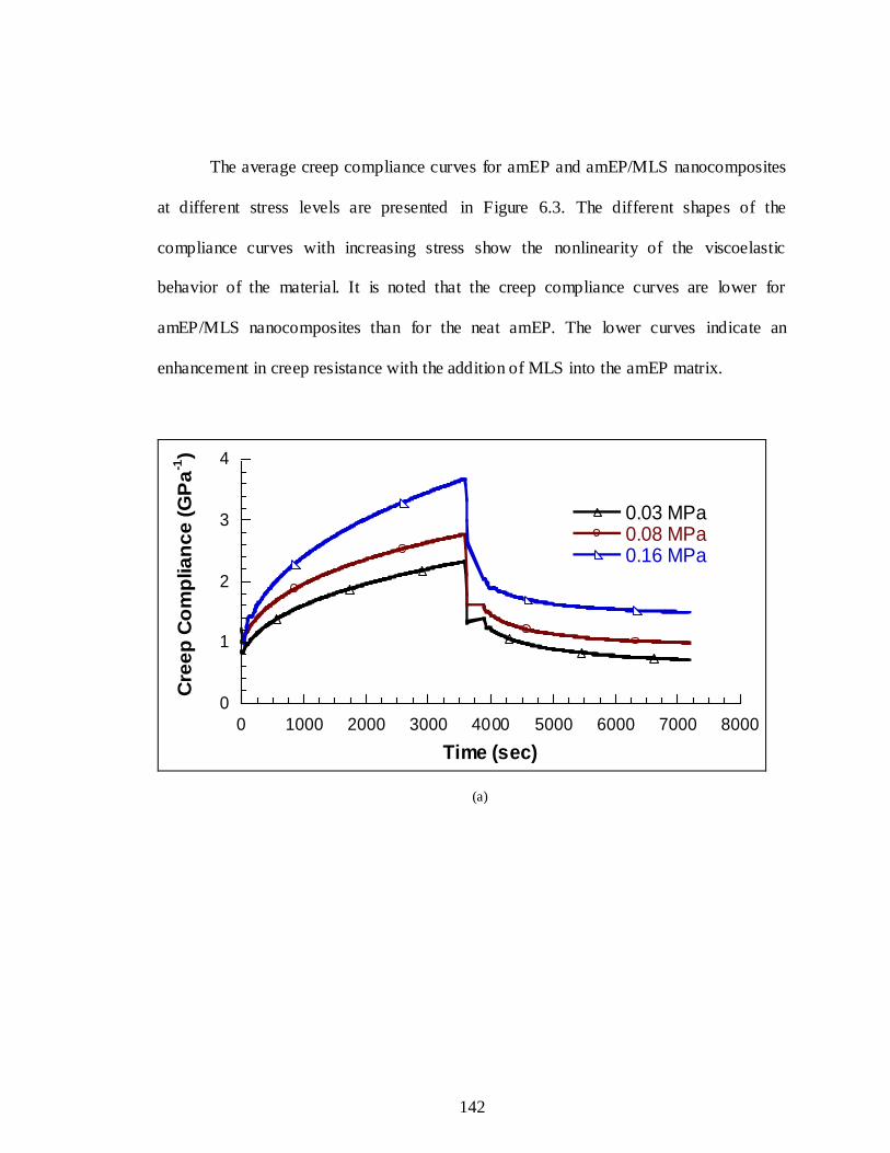
142
The average creep compliance curves for amEP and amEP/MLS nanocomposites
at different stress levels are presented in Figure 6.3. The different shapes of the
compliance curves with increasing stress show the nonlinearity of the viscoelastic
behavior of the material. It is noted that the creep compliance curves are lower for
amEP/MLS nanocomposites than for the neat amEP. The lower curves indicate an
enhancement in creep resistance with the addition of MLS into the amEP matrix.
0
1
2
3
4
0 1000 2000 3000 4000 5000 6000 7000 8000
0.03 MPa0.08 MPa0.16 MPa
Cre
ep
Co
mp
lia
nc
e (
GP
a-1
)
Time (sec)
(a)

143
0
1
2
3
4
0 1000 2000 3000 4000 5000 6000 7000 8000
0.04 MPa0.09 MPa0.18 MPa
Cre
ep
Co
mp
lia
nc
e (
GP
a-1
)
Time (sec)
(b)
0
1
2
3
4
0 1000 2000 3000 4000 5000 6000 7000 8000
0.05 MPa0.11 MPa0.21 MPa
Cre
ep
Co
mp
lia
nc
e (
GP
a-1
)
Time (sec)
(c)
Figure 6.3. Creep compliance versus time plot of LLDPE nanocomposites: (a) amEP, (b) amEP/1% MLS, (c) amEP/3% MLS at room temperature.

144
The nonlinear creep model based on the time-stress superposition principle was
also applied for the description of the creep data of the amEP nanocomposites. The creep
compliance curves at the different stress levels were shifted horizontally to obtain the
smooth mastercurves shown in Figure 6.4. As expected, no vertical shifting was applied
because of the amorphous nature of amPE. As seen from Figure 6.4, the addition of 1%
MLS into amEP led to a significant enhancement in the material creep resistance. The
highest creep resistance was obtained for the addition of 3% MLS.
0.00
0.50
1.00
1.50
2.00
2.50
3.00
3.50
4.00
1.E+01 1.E+02 1.E+03 1.E+04 1.E+05 1.E+06
D (
GP
a-1
)
log t (sec)
amEP
amEP/MLS 1
amEP/MLS 3
Figure 6.4. Mastercurve of linear transient compliance at 25 oC of amEP/MLS nanocomposites.
6.3.2 Schapery Modeling Parameters
The successful superposition of a mastercurve of the LLDPE nanocomposites
indicates that the creep tests of LLDPE nanocomposites can be accelerated by increasing
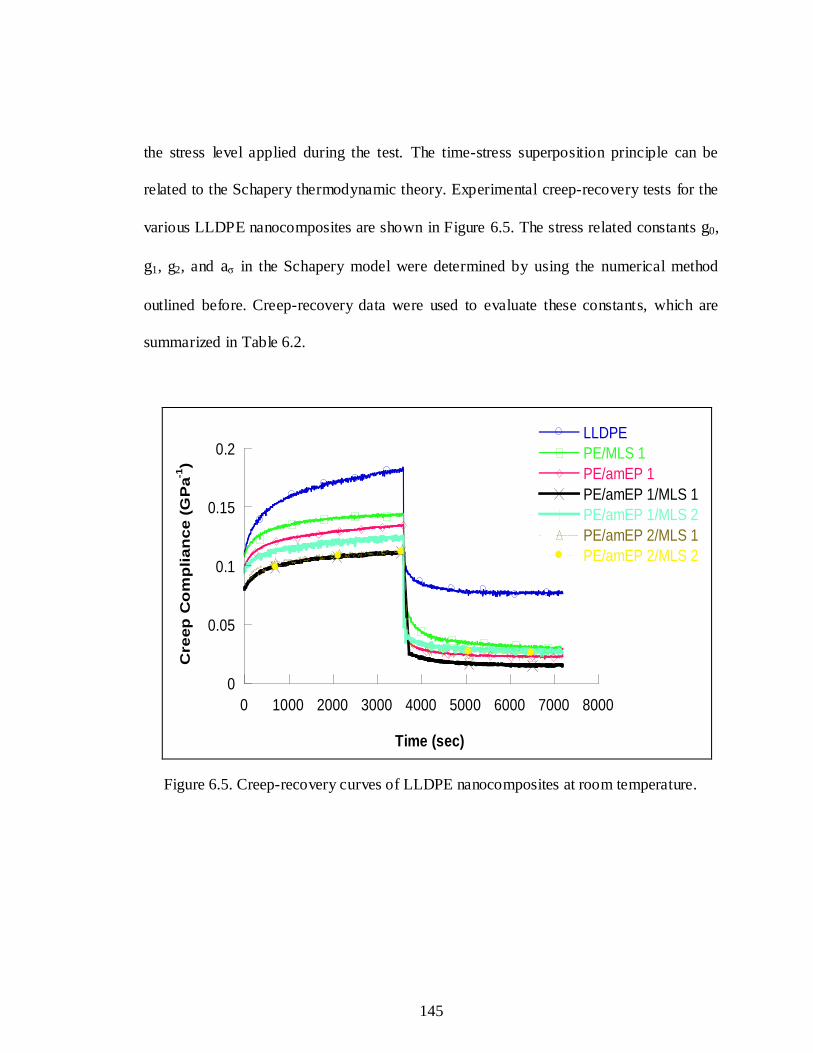
145
the stress level applied during the test. The time-stress superposition principle can be
related to the Schapery thermodynamic theory. Experimental creep-recovery tests for the
various LLDPE nanocomposites are shown in Figure 6.5. The stress related constants g0,
g1, g2, and aσ in the Schapery model were determined by using the numerical method
outlined before. Creep-recovery data were used to evaluate these constants, which are
summarized in Table 6.2.
0
0.05
0.1
0.15
0.2
0 1000 2000 3000 4000 5000 6000 7000 8000
LLDPE
PE/MLS 1
PE/amEP 1
PE/amEP 1/MLS 1
PE/amEP 1/MLS 2
PE/amEP 2/MLS 1
PE/amEP 2/MLS 2
Cre
ep
Co
mp
lia
nc
e (
GP
a-1
)
Time (sec)
Figure 6.5. Creep-recovery curves of LLDPE nanocomposites at room temperature.
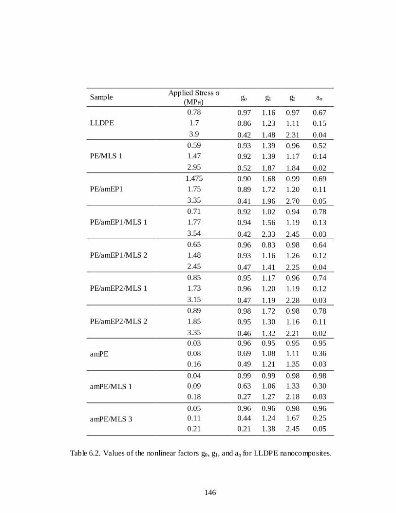
146
Sample Applied Stress σ
(MPa) go g1 g2 aσ
LLDPE
0.78 0.97 1.16 0.97 0.67
1.7 0.86 1.23 1.11 0.15
3.9 0.42 1.48 2.31 0.04
PE/MLS 1
0.59 0.93 1.39 0.96 0.52
1.47 0.92 1.39 1.17 0.14
2.95 0.52 1.87 1.84 0.02
PE/amEP1
1.475 0.90 1.68 0.99 0.69
1.75 0.89 1.72 1.20 0.11
3.35 0.41 1.96 2.70 0.05
PE/amEP1/MLS 1
0.71 0.92 1.02 0.94 0.78
1.77 0.94 1.56 1.19 0.13
3.54 0.42 2.33 2.45 0.03
PE/amEP1/MLS 2
0.65 0.96 0.83 0.98 0.64
1.48 0.93 1.16 1.26 0.12
2.45 0.47 1.41 2.25 0.04
PE/amEP2/MLS 1
0.85 0.95 1.17 0.96 0.74
1.73 0.96 1.20 1.19 0.12
3.15 0.47 1.19 2.28 0.03
PE/amEP2/MLS 2
0.89 0.98 1.72 0.98 0.78
1.85 0.95 1.30 1.16 0.11
3.35 0.46 1.32 2.21 0.02
amPE
0.03 0.96 0.95 0.95 0.95
0.08 0.69 1.08 1.11 0.36
0.16 0.49 1.21 1.35 0.03
amPE/MLS 1
0.04 0.99 0.99 0.98 0.98
0.09 0.63 1.06 1.33 0.30
0.18 0.27 1.27 2.18 0.03
amPE/MLS 3
0.05 0.96 0.96 0.98 0.96
0.11 0.44 1.24 1.67 0.25
0.21 0.21 1.38 2.45 0.05
Table 6.2. Values of the nonlinear factors g0, g1, and aσ for LLDPE nanocomposites.

147
The stress shift factors g0 and g1 are determined from the creep data by fitting the
creep strain to Schapery’s equations derived in chapter 2. Figure 6.6 shows the
comparison between creep and recovery experimental data and the Schapery model
predictions. The values of g2 and aσ were determined by fitting the recovery data to
Schapery’s recovery equation for each stress level applied. It is worth mentioning that the
resulting n-values were more reliably obtained from creep rather than recovery data as
proposed by Augl [23]. The n values were then used to analyze the others parameters by
using recovery the Equation.
0.06
0.08
0.1
0.12
0.14
0.16
0.18
0.2
0 1000 2000 3000 4000 5000
LLDPE (Experimental)
LLDPE (Schapery Model)
PE/MLS 1 (Experimental)
PE/MLS 1 (Schapery Model)
PE/amEP 1 (Experimental)
PE/amEP 1 (Schapery Model)
PE/amEP 1/MLS 1 (Experimental)
PE/amEP 1/MLS 1 (Schapery Model)
PE/amEP 1/MLS 2 (Experimental)
PE/amEP 1/MLS 2 (Schapery Model)
PE/amEP 2/MLS 1 (Experimental)
PE/amEP 2/MLS 1 (Schapery Model)
PE/amEP 2/MLS 2 (Experimental)
PE/amEP 2/MLS 2 (Schapery Model)
Cre
ep
Co
mp
lian
ce (
GP
a-1
)
Time (sec)
(a)

148
0
0.02
0.04
0.06
0.08
0.1
0.12
0.14
4000 5000 6000 7000 8000 9000
LLDPE (Experimental)
LLDPE (Schapery Model)
PE/MLS 1 (Experimental)
PE/MLS 1 (Schapery Model)
PE/amEP 1 (Experimental)
PE/amEP 1 (Schapery Model)
PE/amEP 1/MLS 1 (Experimental)
PE/amEP 1/MLS 1 (Schapery Model)
PE/amEP 1/MLS 2 (Experimental)
PE/amEP 1/MLS 2 (Schapery Model)
PE/amEP 2/MLS 1 (Experimental)
PE/amEP 2/MLS 1 (Schapery Model)
PE/amEP 2/MLS 2 (Experimental)
PE/amEP 2/MLS 2 (Schapery Model)
Re
co
very
Co
mp
lia
nce
(G
Pa
-1)
Time (sec)
(b)
Figure 6.6. Experimental and theoretical (Schapery model) comparison of (a) creep
compliance and (b) recovery compliance.
Following the steps described, each of the Schapery nonlinear parameters was
separately estimated. Each of the parameters has a specific physical meaning. The
parameter g0 is a measure of the stress dependence of the initial time-independent
component of the compliance D0. Parameter g1 expresses the stress dependence of the
transient, time dependent component of the compliance ΔD (ψ- ψ’). Parameter g2 reflects
the effect of loading rate on the time-dependent response of the material and depends on
both stress and temperature, and aσ is a shift factor superimposing the creep curves on a
general master curve.

149
A graphical representation of the g0 variation versus the applied stress is shown in
Figure 6.7. The decreasing values of g0 with increasing stress levels denote a material
hardening occurring because of the application of load. The values of g0 are lower in
samples containing a combination of amEP and MLS. This indicates a material
reinforcing effect with the addition of amEP and MLS which is reflected in higher
modulus and strength for LLDPE nanocomposites as compared to the pure LLDPE
matrix. The values have noticeable variations at higher stresses, where the applied stress
values are close to the elastic limit.
0.1 0.2 0.3 0.4 0.50.2
0.4
0.6
0.8
1
g 0
y (MPa/MPa)
LLDPE
PE/MLS 1
PE/amEP 1
PE/amEP 1/MLS 1
PE/amEP 1/MLS 2
PE/amEP 2/MLS 1
PE/amEP 2/MLS 2
amEP
amEP/MLS 1
amEP/MLS 3
Figure 6.7. Stress dependence of the stress shift factor g0.

150
The g1 values represent the part of creep that is recoverable after the load has been
removed. In that sense, it is a stress-dependent factor. A high value of g1 suggests
quickness in recovery. It is observed that the values of g1 increase with the applied stress
for all compositions as shown in Figure 6.8. The relative increase is higher when MLS is
added compared to pure LLDPE. The g1 value is further increased with the addition of
amPE. This increase can be related to the addition of an elastic matrix which acts to
improve the elastic recovery of the material. The maximum increase in g1 is seen for
compositions containing a 1:1 ratio of amEP and MLS. For amEP nanocomposites, the
addition of 1% MLS shows a small increase in g1 values. The addition of 3% MLS into
amEP shows a further increase with respect to amEP at all stress levels. The results
support the previous observations in which the addition of MLS acts to increase the g1
values of LLDPE nanocomposites. The lower values of g1 values for amEP as compared
to LLDPE are explained by the amorphous nature of the matrix.

151
0.1 0.2 0.3 0.4 0.50.5
1
1.5
2
2.5g 1
y (MPa/MPa)
LLDPE
PE/MLS 1
PE/amEP 1
PE/amEP 1/MLS 1
PE/amEP 1/MLS 2
PE/amEP 2/MLS 1
PE/amEP 2/MLS 2
amEP
amEP/MLS 1
amEP/MLS 3
Figure 6.8. Stress dependence of the stress shift factor g1.
Using the recovery equation in Schapery’s model, the recovery test data for each
recovery experiment were fitted in order to obtain the values of aσ. The values of aσ are
plotted as a function of the applied stress in Figure 6.9. The values are less than 1,
indicating that the reduced time is greater than the real time. This finding suggests that
higher stress will cause the material to accelerate its creep behavior. Figure 6.9 shows
that the values of aσ are largely material dependent. These factors are structure dependent
and are obtained from analyzing experimental results. Since they are material dependent,
they will change from one sample to another. Also, due to their correspondence with the
structure of the material, they can indicate the degree of linearity and non- linearity of the
system. The addition of a combination of amEP and MLS shows lower values indicating

152
a decrease in the non- linear dependence of the creep of the material and hence
improvement of the creep resistance.
0.1 0.2 0.3 0.4 0.50.01
0.1
1
a
y (MPa/MPa)
LLDPE
PE/MLS 1
PE/amEP 1
PE/amEP 1/MLS 1
PE/amEP 1/MLS 2
PE/amEP 2/MLS 1
PE/amEP 2/MLS 2
amEP
amEP/MLS 1
amEP/MLS 3
Figure 6.9. Stress dependence of the stress shift factor aσ.
The values of g2 represent the response of the material with no stress applied
(recovery). Comparing g2 and the product of g1 and g2 allows the separation of stress
effects during creep from material effects during recovery. Figure 6.10 shows the
variation of g2 for LLDPE nanocomposites with the applied stress. It can be seen that the
magnitude of g2 increases with the applied stress for all LLDPE samples. This shows that
the behavior the specimens during recovery with no stress applied is mater ial dependent
.It is observed that the values of g2 are higher when MLS is added as compared to pure
LLDPE. The addition of amEP serves to increase the values. The values of g2 for all
compositions containing a combination of amEP and MLS are higher than these

153
containing amEP and MLS separately. For amEP nanocomposites, the same trend is
observed in g2 values. For compositions containing 1% MLS, the g2 values are higher
than for the neat amPE. The addition of 3% MLS further increases the g2 values for all
stress levels. This implies that the addition of low concentrations of amEP and MLS leads
to a different structure in recovering. The results can be explained by structural
differences induced with the addition of amEP and MLS, and reinforces the initial theory
about addition of amEP and MLS. The addition of amEP increases the strength of the
system, leading to a more ductile material that will undergo a higher degree of
deformation. This has been noted at all the stages of the mechanical testing. The addition
of low concentrations of MLS increases the stiffness of the matrix and shows lower
compliance in comparison with the PE and PE + amEP samples.

154
0.1 0.2 0.3 0.4 0.50.8
1.2
1.6
2
2.4
2.8
g2
y (MPa/MPa)
LLDPE
PE/MLS 1
PE/amEP 1
PE/amEP 1/MLS 1
PE/amEP 1/MLS 2
PE/amEP 2/MLS 1
PE/amEP 2/MLS 2
amEP
amEP/MLS 1
amEP/MLS 3
Figure 6.10. Stress dependence of the stress shift factor g2.
6.4 Conclusions
The tensile behavior and long-term creep of LLDPE nanocomposites were
investigated. The creep behavior of the polymer was viscoelastic, and the nonlinearity in
stress was revealed by investigating the creep compliance of the material at different
stress levels. The creep compliance mastercurves can be used to predict the long-term
creep behavior of the nanocomposites.
A considerable enhancement in the creep resistance was obtained with the
addition of amEP and MLS when compared with the pure LLDPE and was revealed by
comparing the stress-dependent mastercurves. The Schapery nonlinear model was used to
model the creep behavior of the nanocomposites with respect to stress. The absolute

155
values of the stress factors indicated an enhanced creep resistance in the nanocomposites
as compared with the neat PE and amEP matrix.
6.5. References
1. J.L. Yang, Z. Zhang, A. Schlarb, and K. Friedrich, Polymer, 47, 2791-2801 (2006).
2. K.Maniar, Polymer-Plastics Technology and Engineering, 43, 427-443 (2004).
3. A. Ranade, K. Nayak, D. Fairbrother, and N.A. D’Souza, Polymer, 46, 7323-7333
(2005).
4. J.L. Yang, Z. Zhang, A. Schlarb, and K. Friedrich, Polymer, 47, 2791-2801 (2006).
5. M. Niaounakis and E. Kontou, J. Polym. Sci.: Part B: Polymer Physics, 43, 1712-1727
(2005).
6. G. Liang, J. Xu, S. Bao, and W. Xu, J. Appl. Polym. Sci., 91, 3974-3980 (2004).
7. A. Pegoretti, J. Kolarik, C. Peroni, C. Migliaresi, Polymer, 4, 2751-2759 (2004).
8. D. Vlasveld, H. Bersee, and S.J. Picken., Polymer, 46, 10279-10289 (2005).
9. J. Sterling and J. Rand, Biaxial Stress Limit for ULDB Film. AIAA 5th Aviation,
Technology,
Integration, and Operations Conference, Arlington, Virginia (2005).
10. J. Sterling and J. Rand, Advances in Space Research, 37, (2006).
11. J. Rand, J. Henderson, and D. Grant. Polym. Eng. and Sci., 36, 1058-1064 (1996).
12. G. Papanicolaou, S. Zaoutsos, and A. Cardon, Composites Science and Technology,
58, 883-
889 (1998).
13. G. Papanicolaou, S. Zaoutsos, and A. Cardon, Composites Science and Technology,
59,
1311-1319 (1999).
14. D. Touatl and G. Cederbaum, J. Eng. Mat. and Tech., 119: 121 (1997).
15. A. Luna and N. D’Souza. ANTEC 2000: Plastics, the Magical Solution: Conf. Proc.,
May 7-11, Orlando, Florida (2000).

156
16. J. Lai and A. Bakker, Polym. Eng. and Sci., 36, 1058-1064 (1995).
17. L.C.E. Struik , Physical aging in amorphous polymers and other materials, Elsevier:
New
York (1978).
18. M. Tajvidi, R. Falk, and J. Hermanson, J. Appl. Polym. Sci., 97, 1995-2004 (2005).
19. M Elahi and Y. Weitsman, Mechanics of Time-Dependent Material, 3, 219–244
(1999).
20. D. Pooler and L. Smith, J. Thermoplastic Composite Mat., 17, 427-445 (2004).
21. A Pramanick and M Sain, J. Thermoplastic Composite Mat., 19, 35-59 (2006).
22. S. Onogi, T. Sato, T. Asada, and Y. Fukui, J. Polym. Sci., Part A-2 (Polymer
Physics), 8,
1195-1209 (1970).
23. J. Augl, J. Rheol., 31, 1-36 (1987).
157
CHAPTER 7
SEPARATION OF STRUCTURAL TIME DEPENDENT DEFORMATION DUE TO
TEMPERATURE
7.1. Introduction
Polymer nanocomposites reinforced with montmorillonite layered silicate (MLS)
have generated enormous interest in science and engineering in the last years. The time-
independent mechanical properties of polymer–MLS nanocomposites have been well
investigated [1-3] .In most practical applications, compliance of the polymeric material
not only depends on stress but also on time and temperature and hence the time-
temperature dependent response, i.e., creep behavior, is of immense significance [4,5]
The theoretical background for creep behavior of solid polymers is well studied within
the framework of linear viscoelasticity [3,6] .This theory assumes that the creep
compliance is only a function of time and not of strain and stress. But beyond a certain
strain limit compliance became a function of time and stress (or strain). This non-linear
viscoelastic behavior plays a key role in most applications and the data analysis in this
region is more difficult than in the linear region, which has a direct relation to the deeper
understanding of the micromechanical processes controlling the mechanical response [7].
In the past decade, the nonlinear viscoelastic creep behavior of polyethylene
nanocomposites has been studied. [8-10]. Although the time dependent linear and
nonlinear response of polyethylene nanocomposites has been investigated in a number of
publications, the effect of temperature on the mechanical properties of LLDPE

158
nanocomposites has not yet been studied in detail. Tajvidi et al. [11] studied the nonlinear
creep behavior of high density polyethylene (HDPE)/Kenaf fiber composites under
varying temperature. The time–temperature superposition principle was applied to
investigate the viscoelastic properties of a composite of 50% kenaf fibers, 48% HDPE,
and 2% compatibilizer. Creep data were shifted horizontally and vertically, and a master
curve was constructed. The results indicated that the composite material was
thermorheologically complex, and a single horizontal shift was not adequate to predict
the long-term performance of the material. Pramanick et al. [12] studied the temperature-
stress equivalency in nonlinear viscoelastic creep characterization of high density
polyethylene (HDPE) composites. The combined effect of temperature and stress on
creep strain was accommodated in a single analytical function where the interaction was
shown to be additive.
In our previous work, we investigated the nonlinear creep compliance of LLDPE
nanocomposites at room temperature using Schapery nonlinear model [13]. A
considerable enhancement in the creep resistance was obtained with the addition of amEP
and MLS when compared with the pure LLDPE and was revealed by comparing the
stress dependent mastercurves. Schapery nonlinear equation was used to model the creep
behavior of the nanocomposites with respect to stress. The absolute values of the stress
factors indicated an enhanced creep resistance in the nanocomposites as compared with
the neat PE and amEP matrix. In this paper, we investigate the temperature dependence
of the nonlinear creep compliance of LLDPE nanocomposites. Time-temperature-stress
superposition principles (TTSSP) similar to time-temperature superposition principles
159
(TTSP) were used to form a “master curve”. The amplitude of compliance was found to
be a function of both stress and temperature which implies that the material is not
“thermorheologically simple”.
7.2. Calculation of Temperature-Related Creep Variables
D0: The initial compliance value can be determined from the instantaneous deflection
data of the creep/time curve in the linear region.
h0 : According to Equation 38 in chapter 2, h0 could be calculated from creep plot when t
is equal to zero. The following equation can be used to calculate the compliance
0
000
)0()0()0(
DhhDD
h1 : h1 can be calculated by curve fitting of recovery strain data to Equation 41 in chapter
2 and using the following equation
Ah
hA aa
1
1
aT: The numerical estimation of aT can be done by fitting the recovery strain data to
Equation 38 in chapter 2.
h2 : h2 can be calculated from the following equation where the assumption is that h2=1 in
the linear region:
2
11
1 hhC
an
T

160
7.2.1. Temperature Shift Factor
Temperature may influence compliance in a similar way as stress. Temperature
effects can be described by changing the timescale of the viscoelastic response. Thus, if
D is the compliance at a temperature T1 and time t, the creep compliance at a temperature
T2 can be described as follows:
),/(),( 21 TatgDTtD T
Where aT is the temperature shift factor.
For thermorheologically complex materials such as semicrystalline material, a
vertical shift factor of the data plots along the y-axis should be considered [14]. The
concept of the vertical shift factor has been used by many authors [15-17]. While the real
cause of the vertical shift is not clear, it is thought it is a representation of the change in
crystallinity [18]. Furthermore, the temperature dependent shift factor aT is related to the
activation energy Ea as follows
ref
a
TTTR
Ea
11
303.2log
where R is the universal gas constant. The activation energy can be obtained from the
slope of the curve of aT against 1/T.

161
7.3. Experimental
7.3.1. Materials
LLDPE DOWLEX 2056G (Dow chemical company) was used to prepare the PE
nanocomposite films (density = 0.92 g/cc; Melt index = 1.0 gm/10 min).
Montmorillonite- layered silicate (MLS) (Cloisite 15A™), supplied by southern clay
products, was used as the nanofiller. An amorphous maleic anhydride functionalized
elastomeric copolymer, Exxelor VA 1803 (ExxonMobil corporation), was used as a
compatibilizer between the MLS and the PE matrix. Exxelor VA 1803 has a nominal
density of 0.86 g/cm3 and a melt index of 3 g/10 min (ASTM D1238, 230 oC, 2.16 kg).
The maleic anhydride (MA) level is in the range of 0.5 to 1%.
7.3.2. Sample Preparation
Nanocomposites were compounded with a Haake TW100 twin-screw extruder
with a temperature profile of 200, 200, 205, and 210 oC for zones 1 to 4, respectively. PE
films 1.5 mil (0.04 mm) thick were processed with a Killion single-screw extruder (L/D =
24:1), fitted with a dual- lip air ring and a die diameter of 50 mm (2 inches). Blends of
PE+amPE+MLS were made, and the mixtures were compounded and pelletized. The
compounded pellets were then processed into a blown film. . Table 7.1 summarizes the
concentrations used.

162
Sample LLDPE
(wt %)
Exxelor VA 1803
(wt %)
MLS
(wt %)
LLDPE 100 0 0
PE/MLS 1 99 0 1
PE/amEP1 99 1 0
PE/amEP1/MLS 1 98 1 1
Table 7.1. Summary of compositions used.
7.3.3. Creep Testing
Uniaxial tensile creep tests were performed using RSA III with the films
attachment. The desired constant stress to be applied for each measurement is calculated
to be 50% of the yield stress. The constant stress is applied for 1 hour of loading followed
by 1 hour of unloading. A linear displacement transducer with a force capacity of 35 N is
used to monitor the strain during the experiment. Creep tests were performed at the same
set of temperatures as the tensile tests. The effect of temperature on creep was studied by
running experiments at different temperatures of 25, 10, -10, -30, -50, -70, and -90 oC. A
convection oven with a temperature range of -150 oC to 600 oC was used for this purpose.
7.4. Results and Discussion
7.4.1. Time/Temperature Equivalence
The effect of temperature on the nonlinear creep behavior of the LLDPE
nanocomposites was investigated. The temperature was varied from -90 to 25 oC with a
20 oC interval. Figure 7.1 shows the creep behavior of LLDPE nanocomposites at
different temperatures. The stress levels in the creep tests were chosen based on the
results of the tensile tests and did not exceed 0.5 of the ultimate yield point. Since the

163
stress region is far from the yield point, it is assumed that the primary deformation
mechanism for the materials in creep was of viscoelastic nature, while the contribution of
plastic strains was insignificant in the stress and time ranges considered.
0
0.05
0.1
0.15
0.2
0 1000 2000 3000 4000 5000 6000 7000 8000
25 oC
-10 oC
10 oC
-30 oC
-50 oC
-70 oC
-90 oC
Cre
ep
Co
mp
lia
nc
e (
GP
a-1
)
Time (sec)
(a)

164
0
0.02
0.04
0.06
0.08
0.1
0.12
0.14
0 1000 2000 3000 4000 5000 6000 7000 8000
25oC
10 oC
-10 oC
-30 oC
-50 oC
-70 oC
-90 oCC
re
ep
Co
mp
lian
ce
(G
Pa
-1)
Time (sec)
(b)
0
0.05
0.1
0.15
0 1000 2000 3000 4000 5000 6000 7000 8000
25 oC
10 oC
-10 oC
-30 oC
-50 oC
-70 oC
-90 oC
Cre
ep
Co
mp
lia
nc
e (
GP
a-1
)
Time (sec)
(c)

165
0
0.02
0.04
0.06
0.08
0.1
0.12
0 1000 2000 3000 4000 5000 6000 7000 8000
25 oC
10 oC
-10 oC
-30 oC
-50 oC
-70 oC
-90 oC
Cre
ep
Co
mp
lian
ce
( G
Pa
-1 )
Time (sec)
(d)
Figure 7.1. Creep-recovery of LLDPE nanocomposites (a) pure LLDPE (b) PE/1% MLS (c) PE/1% amEP(d) PE/1% amEP/1% MLS at different temperatures.
From Figure 7.1, it can be seen that the creep compliance of LLDPE
nanocomposites is temperature dependent. The creep compliance curves increase with
increasing temperature. This indicates that LLDPE nanocomposites exhibit a strong non-
linear behavior with temperature similar to the stress dependence discussed in our
previous study [13]. The non- linearity observed in temperature suggests that the time-
temperature-stress-superposition principle (TTSSP) can be applied to LLDPE
nanocomposites. According to this principle, long term creep deformation can be
predicted based on short-term creep data at different temperatures and stress levels by a
time-shifting method. It should be noted that at isothermal conditions, the TTSSP reduces
to the time-stress-superposition principle (TSSP) used before. Horizontal and vertical
166
shifting was applied to construct the temperature dependent mastercurve of the LLDPE
nanocomposites.
Figure 7.2 shows the temperature-dependent mastercurves of all samples. The
mastercurves obtained could predict the creep behavior of the materials for a period of
time more than 60 times exceeding the test time. From Figure 7.2, it can be seen that the
creep compliance decreases with the addition of MLS. The addition of amEP further
decreases the creep compliance. Strikingly, the nanocomposite with 1% amEP and 1%
MLS exhibited the lowest compliance, i.e., the highest creep resistance. These
observations led to a fundamental aspect for understanding the creep behavior of LLDPE
nanocomposites. The creep response is controlled by the good interaction between amEP
and MLS in the LLDPE nanocomposite.

167
0.00
0.05
0.10
0.15
0.20
0.25
0.30
1.0E-02 1.0E-01 1.0E+00 1.0E+01 1.0E+02 1.0E+03 1.0E+04 1.0E+05 1.0E+06 1.0E+07 1.0E+08
D(t
)-D
(0),
GP
a-1
Log Reduced Time (sec)
PE/amEP 1/MLS 1
LLDPE
PE/MLS 1
PE/amEP 1
Figure 7.2. The temperature dependent creep compliance mastercurve.
7.4.2. Modeling Parameters of Schapery Model
The successful superposition of a mastercurve of the LLDPE nanocomposites
indicates that the creep tests of LLDPE nanocomposites can be accelerated by
increasing/decreasing the temperature/stress during the creep test. The time-temperature-
stress superposition principle can be related to the Schapery thermodynamic theory. The
temperature related constants h0, h1, h2, and aT in the Schapery model were determined by
using the numerical method outlined before. Creep-recovery data were used to evaluate
these constants, which are summarized in Table 7.2.

168
Sample Temperature
(oC)
Applied Stress
(MPa) ho h1 h2 aT
LLDPE
10 1.69 0.96 0.54 0.88 0.243
-10 3.16 0.96 0.78 1.26 0.135
-30 4.66 0.95 1.39 1.40 0.069
-50 6.34 0.96 1.47 1.50 0.005
-70 7.71 0.96 1.57 1.75 0.002
-90 13.5 0.96 1.98 2.10 0.001
PE/MLS 1
10 4.85 0.95 1.11 0.93 0.129
-10 5.08 0.94 1.12 1.23 0.059
-30 6.58 0.96 1.23 1.33 0.008
-50 9.80 0.95 1.25 1.52 0.002
-70 9.80 0.95 1.3 1.68 0.001
-90 11.84 0.96 1.3 2.21 0.001
PE/amEP1
10 2.34 0.96 1.08 0.89 0.622
-10 2.61 0.95 1.26 1.31 0.251
-30 4.64 0.96 1.3 1.39 0.109
-50 8.14 0.95 1.38 1.52 0.088
-70 14.23 0.95 1.57 1.76 0.058
-90 24.67 0.96 1.58 2.05 0.008
PE/amEP1/MLS 1
10 5.35 0.95 0.92 0.98 0.405
-10 6.85 0.95 1.05 1.30 0.248
-30 8.50 0.95 1.1 1.42 0.064
-50 12.25 0.95 1.16 1.68 0.026
-70 17.35 0.96 1.24 1.76 0.005
-90 22.77 0.94 1.49 2.27 0.001
Table 7.2. Values of the nonlinear factors h0, h1, and aT for LLDPE nanocomposites at
different temperatures.

169
Following the steps described, each of the Schapery nonlinear parameters was
separately estimated. Each of the parameters has a specific physical meaning. The
parameter h0 is a measure of the stress dependence of the initial time-independent
component of the compliance D0. Parameter h1 expresses the stress dependence of the
transient, time dependent component of the compliance ΔD. Parameter h2 reflects the
effect of loading rate on the time-dependent response of the material and depends on both
stress and temperature, and aT is a shift factor superimposing the creep curves on a
general master curve.
Figure 7.3 shows the variation of h0 with temperature. It can be seen that the value
of h0 does not show significant change with temperature for all compositions tested. This
implies a linear temperature dependent creep behavior of LLDPE nanocomposites.

170
0
0.2
0.4
0.6
0.8
1
-100 -80 -60 -40 -20 0 20
LLDPE
PE/MLS 1PE/amEP 1
PE/amEP 1/MLS 1
h0
Temperature (oC)
Figure 7.3. Variation of temperature dependent creep constant h0 with temperature.
The h1 values represent the part of creep that is recoverable after the load has
been removed. In that sense, it is a stress dependent factor. A higher value of h1 suggests
quickness in recovery. It is observed that the values of h1 increase with temperature for
LLDPE as shown in Figure 7.4. The same relative increase with temperature is observed
when MLS is added to pure LLDPE. The h1 value is further increased with the addition
of amEP. This can be related to the addition of an elastic matrix which acts to improve
the elastic recovery of the material at lower temperatures. The h1 values for compositions
containing a 1:1 ratio of amEP and MLS also show an increase suggesting an
improvement in the creep resistance with decreasing temperature.

171
0
0.5
1
1.5
2
2.5
10 -10 -30 -50 -70 -90
h1
Temperature (oC)
LLDPE PE/MLS 1 PE/amEP 1 PE/amEP 1/MLS 1
Figure 7.4. Variation of temperature dependent creep constant h1 with temperature.
The values of h2 represent the response of the material with no stress applied
(recovery). This allows the separation of stress effects during creep from material effects
during recovery. Figure 7.5 shows the variation of h2 for LLDPE nanocomposites with
temperature. It can be seen that the magnitude of h2 increases with temperature for all
LLDPE samples. It is observed that the values of h2 are higher when MLS is added as
compared to pure LLDPE. The addition of amEP serves to increase the values. The
values of h2 for all compositions containing a combination of amEP and MLS are higher
than these containing amEP and MLS separately. This implies that the addition of low
concentrations of amEP and MLS leads to a different structure in recovering. The results
can be explained by structural differences induced with the addition of amEP and MLS,
and reinforces the initial theory about addition of amEP and MLS. The addition of amEP
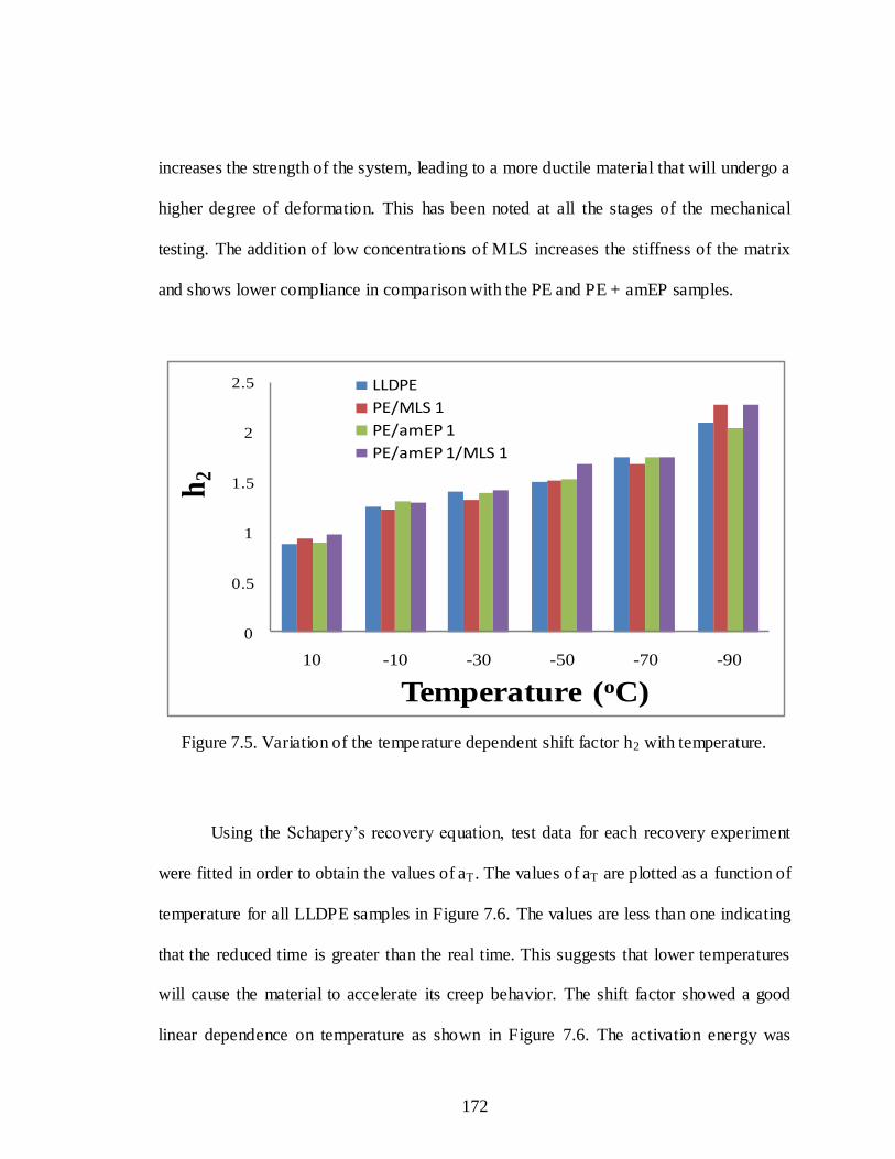
172
increases the strength of the system, leading to a more ductile material that will undergo a
higher degree of deformation. This has been noted at all the stages of the mechanical
testing. The addition of low concentrations of MLS increases the stiffness of the matrix
and shows lower compliance in comparison with the PE and PE + amEP samples.
0
0.5
1
1.5
2
2.5
10 -10 -30 -50 -70 -90
h2
Temperature (oC)
LLDPE
PE/MLS 1
PE/amEP 1
PE/amEP 1/MLS 1
Figure 7.5. Variation of the temperature dependent shift factor h2 with temperature.
Using the Schapery’s recovery equation, test data for each recovery experiment
were fitted in order to obtain the values of aT . The values of aT are plotted as a function of
temperature for all LLDPE samples in Figure 7.6. The values are less than one indicating
that the reduced time is greater than the real time. This suggests that lower temperatures
will cause the material to accelerate its creep behavior. The shift factor showed a good
linear dependence on temperature as shown in Figure 7.6. The activation energy was

173
obtained by the slope of a plot of log aT against 1/T. The calculated values are listed in
Table 7.3.
0
0.1
0.2
0.3
0.4
0.5
0.6
0.7
-100 -80 -60 -40 -20 0 20
aT
Temperature (oC)
LLDPE
PE/MLS 1
PE/amEP 1
PE/amEP 1/MLS 1
Figure 7.6. Variation of the shift factor aT with temperature.
Sample Ea (kJ/mol)
LLDPE 99.13
PE/MLS 1 93.56
PE/amEP1 99.18
PE/amEP1/MLS 1 92.8
Table 7.3. Activation energy of LLDPE nanocomposites obtained from the mastercurves.
The activation energy of the nanocomposites was lower than that of LLDPE,
indicating that mobility of the polymer chains became easier with the addition of MLS.

174
The results are in agreement with dynamic mechanical measurements which show a
decrease in the glass transition temperature with the addition of MLS [19].
7.5. Conclusions
The tensile behavior and long-term creep of LLDPE nanocomposites was
investigated .The creep behavior of the polymer was viscoelastic and the nonlinearity in
temperature was revealed by investigating the creep compliance of the material at
different temperatures. The creep compliance mastercurves can be used to predict the
long term creep behavior of the nanocomposites. A considerable enhancement in the
creep resistance was obtained with the addition of amEP and MLS when compared with
the pure LLDPE and was revealed by comparing the temperature dependent
mastercurves.
Schapery nonlinear model was used to model the creep behavior of the
nanocomposites with respect to temperature. The absolute values of the te mperature
factors also indicated an enhanced creep resistance in the nanocomposites as compared
with the neat PE matrix. The addition of 1:1 ratio of amEP and MLS shows to have the
highest creep resistance among the materials investigated.

175
7.6. References
1. JL Yang, Z Zhang, A Schlarb, K Friedrich, Polymer, 47, 2791-2801 (2006)
2. A Pegoretti, J Kolarik, C Peroni, Cilgiaresi, Polymer, 4, 2751-2759 (2004)
3. Z Zhang, JL Yang, K Friedrich, Polymer, 45, 3481-3485( 2004)
4. JL Yang, Z Zhang, A Schlarb, K Friedrich, Polymer, 47, 6745-6758(2006)
5. J Lai, W Findley, Transactions of the Society of Rheology, 17, 63-87 (1973)
6. LCE Struik , Physical aging in amorphous polymers and other materials; Elsevier:
New York (1978)
7. J Kolarik, A Pegoretti, Polymer, 47, 346-356 (2006)
8. G Liang, J Xu, S. Bao, W. Xu, J. of Appl. Polym. Sci, 91, 3974-3980 (2004)
9. D Martin, P Halley, R Truss, Polym Int., 52, ,1774–1779 (2003)
10. RW Truss, TK Yeow, J. of Appl. Polym. Sci., 100, 3044-3049 (2006)
11. M Tajvidi, R Falk, J Hermanson, Appl. Polym. Sci., 97, 1995-2004 (2005)
12. Pramanick, M Sain, J. of Thermoplastic Composite Mat.,19,35-59 (2006)
13. A Shaito, D Fairbrother, J Sterling, N.A D’Souza, “Nonlinear creep deformation in
polyethylene nanocomposites: Temperature effects”, Polym. Eng. and Sci, submitted
(2008).
14. M Tajvidi, R Falk, J Hermanson, J. Appl. Polym. Sci., 97, 1995–2004 (2005)
15. M Elahi, Y Weitsman, Mechanics of Time-Dependent Material, 3,219–244 (1999)
16. D Pooler, L Smith, J. Thermoplastic Composite Mat.,17,427-445 (2004)
17. A Pramanick, M Sain, J. Thermoplastic Composite Mat.,19,35-59 (2006)
18. S Onogi, T Sato, T Asada, Y Fukui, J. of Polym. Sci., Part A-2 (Polymer
Physics),8,1195-1209 (1970)
19. A Shaito, D Fairbrother, J Sterling, N.A D’Souza, “Nonlinear creep deformation in
polyethylene nanocomposites: stress effects”, Polym. Eng. and Sci, submitted (2008).

176
CHAPTER 8
CONCLUSIONS
The investigation of creep response in polyethylene nanocomposites and correlation
to component contributions, synergistic advantages of their combinations and their stress and
temperature dependent response have been investigated.
In the first section of the study, the tensile and creep properties of the materials
were investigated at room temperature. Tensile results showed the reinforcing effects of
MLS on both LLDPE and amPE. A noticeable increase in elastic modulus (166%) and
yield stress (42%) was obtained with the addition of amEP and MLS to LLDPE. For the
amEP matrix, a 35% increase in yield stress and 90% increase in elastic modulus was
obtained with the addition of 3% MLS. The results suggest MLS to be a good
reinforcement in both the amorphous amEP and the semicrystalline PE. The observed
results from the tensile testing suggest a synergistic effect obtained with the addition of
both amEP and MLS to LLDPE. To assess this, it was important to sort out the possible
effect of different factors on such behavior. These factors include: composition of the
matrix, crystallinity of the matrix, and dispersion of the filler within the matrix. To study
the effect of the composition of the matrix, the ratio of the compatibilizer to the filler was
varied and a set of composition were processed. Among the different compositions, the
1:1 ratio showed the best performance with the highest yield stress and modulus. The
same composition showed the synergistic effects in a previous study by our laboratory.
The yield stress and modulus generally increase with an increase in crystallinity. The

177
crystallization behavior of the nanocomposites was probed using DSC. No change in
crystallinity was observed with the addition of amEP and MLS which negates the
possibility that the observed reinforcement is due to a change in crystallinity. XRD
showed that although no change in crystallinity was obtained with the addition of amEP
and MLS, a thickening of the lamella was observed indicating a change in the
morphology of the matrix.
XRD was then used to study the possible effect of the dispersion of the filler on the
improvement in the tensile properties. The diffractograms of the different composition
showed that increasing the MLS content from 1 % to 2% while keeping the amEP content at
1% decreased the interaction between MLS and the matrix, whereas increasing the degree of
maleation from 1% to 2% causes a collapse of the intergallery chains of the surfactant. An
intercalated/exfoliated system was obtained with the 1:1 ratio sample which suggests that this
composition can be considered as the optimum composition to be used. The XRD of the pure
amorphous amEP showed the disappearance of the MLS characteristic peak which suggested
an intercalated/exfoliated system. To confirm the XRD observations, FIB was uniquely used
to obtain a high resolution image of the dispersed clay platelets. The micrographs of the PE
and amEP nanocomposites showed the good dispersion caused by the addition of amEP when
compared withtheaddition of MLSalone.
Creep test results showed the same behavior observed in the tensile test. The
different compositions were analyzed. A first qualitative analysis of the creep compliance
plots showed the creep resistance improvement caused by the addition of MLS and amEP
separately and combined to the PE matrix. The addition of MLS to the pure amorphous
amEP matrix showed an interesting phenomenon. The MLS acts as a reinforcing agent in
178
amEP as well. Among the different composition, the 1:1 ratio showed the lowest creep
compliance and the lowest unrecoverable deformation. Another qualitative comparison of
the results was done by comparing the creep and recovery plots. The creep plots did not
coincide with the recovery plots indicating a nonlinear viscoelastic behavior which is
attributed to the “undisturbed” amorphous as explained by Struik’s model. The %
recovery was calculated to evaluate the degree of divergence and was found to increase in
the nanocomposites samples.
The dependence of the material properties on structure is defined by considering
Burgers nonlinear viscoelastic model. The structure-property relationship was carried out
by analyzing the fit parameters in this model, since the variations of these parameters
illustrate the influence of the filler on the creep performance of the bulk matrix. From
Burgers model, the most significant parameters to consider are the elastic modulus EM
which is a measure of the instantaneous elastic creep strain and the retardation time τ
which reflects delayed response after removing the applied load. The nanocomposites
showed higher EM values which is a reflection of the improved tensile properties. They
also showed lower retardation times which are an indication of improved elasticity as
compared to the bulk matrix. The amorphous amEP matrix also showed a similar trend,
where EM of the compositions with 1% and 3% MLS where higher than the bulk matrix.
The results confirm the reinforcement characteristics of MLS. An alternative function
that has been successfully used to describe the creep of predominantly semi-crystalline
polymers is based on the KWW function. The parameters from this function are used to
describe the variation of the breadth of relaxation and the characteristic retardation time

179
during the creep process. An increase in the breadth of relaxation is observed for both
amEP and PE nanocomposites which is an indication of a strengthening of the coupling
between the relaxing species and the medium and is related to an overall decrease of the
molecular mobility. The variations of the retardation time from the KWW are in
agreement with those from Burgers model indicating that both functions can be used to
describe the structure-property relation of the nanocomposites.
In the second section of the study, temperature and stress effects on the overall
properties of the nanocomposites were considered. This is of importance due to the fact that
these materials are to be used in structural applications where they experience complex load
and temperature histories, so that is important to design for different stress and temperature
scenarios.
The effect of stress on creep properties of LLDPE nanocomposites was
investigated at room temperature. Like other thermoplastic polymers, polyethylene
exhibits time dependent load response and is characterized as a viscoelastic material. At
low stresses, the stress-strain is independent of stress/strain independent, however, PE is
in general a nonlinear viscoelastic material and the material time dependent properties
cannot be defined by a single creep compliance-time curve and a group of compliance-
time curves at different stress levels are needed to characterize its time-dependent
behavior. In our study, three stress levels of 10, 25, and 50% yield stress were chosen.
The nonlinear time-dependent behavior of the different materials at the different stress
levels were correlated to the fitting parameters of Schapery’s nonlinear equation. The
results showed the time dependent behavior of the different compositions to be nonlinear.

180
The nonlinear behavior was attributed to the “undisturbed” amorphous region far from the
crystals as proposed by Struik. All maleated PE compositions showed a reduction in the
nonlinear response as obtained from Schapery’s fit parameters. The effect of the different
material properties was investigated by normalizing the stress levels applied to the yield
stress of each material. The stress dependent parameter g0 showed a decreasing trend with
increasing stress indicating material hardening. The addition of MLS to PE or the pure
amorphous amEP matrix showed lower values which is an indication of the reinforcement
characteristics of MLS.
The effect of temperature on tensile and creep properties was investigated by
running these tests in the range of -100° to 25°C. The stress level in the creep tests was
kept constant at 50% yield stress ensuring the material response is in the linear
viscoelastic region. The tensile properties of the different compositions at temperatures
below the softening or glass transition temperature show an increasing trend with
decreasing temperature. This is due to the fact that the below the glass transition, the
amorphous and semicrystalline domains are brittle and rigid. For the compositions
considered, the addition of MLS caused an increase in the yield stress and modulus with
decreasing temperature. The maximum increase was obtained for a combination of amEP
and MLS which was the same trend obtained for the room temperature results. These
results showed that MLS acts as a reinforcing agent even at temperatures as low as
-100°C. The molecular relaxation behavior of the bulk PE and amEP matrices can be related
to the yield behavior at low temperatures by considering the dynamic temperature response
of the materials. The storage moduli E’ of the nanocomposites were higher than those of the
pure LLDPE over the entire temperature range. The highest increase in storage modulus

181
(23% at -80°C and 27% at 25°C) was for samples in which a combination of 1% amEP and
1% MLS was used. This increase can be explained by the synergic interaction between amEP
and MLS and is reflected by the tensile test results at these temperatures. The decreased work
hardening evidenced by the drop in stress following UTS in the tensile test results below
-50°C is an indication of a relaxation processes in the matrix. The effect of amEP and MLS
on the viscoelastic properties at different temperatures was investigated by comparing the
variations in tan β peaks of the two relaxation processes. The addition of amEP did not affect
the maxima of the PE for the α transition, indicating no influence of the amorphous
compatibilizer on segmental relaxation, while the addition of MLS hada pronounced effect
on themaxima,supporting the conclusion that MLS provides an interface that affects the
relaxation in the PE matrix.
The effect of temperature on the structure-property relationship was investigated
by considering the variations of the Burgers model and KWW function parameters with
temperature. A similar trend in the creep-recovery behavior at room temperature was
observed with decreasing temperature. All maleated compositions showed increasing %
recovery as compared to the pure PE matrix. It was suggested that MLS particles act as
hingesinthe amorphousmatrixincreasing the elasticity of the bulk matrix. A comparison
of the different parameters from Burgers model showed that all maleated compositions
had higher EM, higher EK and ηK, and lower retardation times for temperature above the
beta transition temperature of PE. The results were related to the reinforcing effect of the
clay particles. Below the β-transition temperature, retardation time increases linearly with
decreasing temperature. This behavior is exhibited because below the beta transition
temperature, the material is in its glassy state where molecular mobility is hindered,

182
reducing the polymer elasticity. The analysis of the KWW parameters showed the same
trend in the retardation times which further confirms the analysis from Burgers model.
The effect of temperature on the nonlinear time dependent behavior was
investigated. In order to evaluate the various functions to modify the linear compliance to
predict the nonlinear response, a set of creep tests were performed at different stresses
and temperatures. The different materials showed a strong nonlinearity with decreasing
temperature similar to that observed with increasing stress levels at room temperature. It
was important to note that the determination of the dependence of the nonlinear strain on
stress and temperature is a key in the design of any linear or nonlinear viscoelastic
material. The different parameter in the Schapery’s model showed to be both stress and
temperature dependent. The values of h2 which represent the response of the material
with no stress applied allowing the separation of stress effects during creep from material
effects during recovery. The magnitude of h2 was shown to increase with temperature for
all LLDPE samples. It was observed that the values of h2 are higher when MLS is added
as compared to pure LLDPE. The addition of amEP serves to increase the values. The
values of h2 for all maleated nanocomposites are higher than these containing amEP and
MLS separately. This implies that the addition of low concentrations of amEP and MLS
leads to a different structure in recovering. The results were explained by structural
differences induced with the addition of amEP and MLS, and reinforce the synergistic
effects of adding amEP and MLS to PE.
The time-temperature superposition principle was successfully used to predict the
long term behavior of LLDPE and amEP nanocomposites. This was important to account

183
for the long term properties from short term tests. Mastercurves for both systems were
constructed. The amorphous nature of amEP was reflected in the use of horizontal shift
factors only, where as horizontal and vertical shift factors were used for the PE material
which is an indication of its semicrystalline nature. Comparing the two master curves, it
was observed that the addition of MLS to both amEP and PE decreased the creep
compliance of the bulk matrix. All maleated PE compositions showed lower creep
compliance. These results further supported the synergistic effect of adding amEP and
MLS separately to the pure LLDPE matrix.
The schematic in Figure 8.1 depicts the prediction of the effect of the
combinations. When montmorillonite is added to a semicrystalline polymer (a), it
typically resides in the amorphous region, perturbing the chains (b). The introduction of a
maleated compatibilizer (c) bridges the polymer to the montmorillonite. Addition of more
compatibilizer (d) does not increase the mechanical performance (2% amEP versus 1%
amEP) because the intrinsic amEP has significantly lower mechanical performance and
beyond offering a chemical bond, limits the incremental mechanical performance of the
composite.

184
Figure 8.1. Schematic explaining material behavior during deformation.