long-term photometric behaviour of outbursting am … · long-term photometric behaviour of...
TRANSCRIPT
MNRAS 446, 391–410 (2015) doi:10.1093/mnras/stu2105
Long-term photometric behaviour of outbursting AM CVn systems
David Levitan,1‹ Paul J. Groot,1,2 Thomas A. Prince,1 Shrinivas R. Kulkarni,1
Russ Laher,3 Eran O. Ofek,4 Branimir Sesar1 and Jason Surace3
1Division of Physics, Mathematics, and Astronomy, California Institute of Technology, Pasadena, CA 91125, USA2Department of Astrophysics/IMAPP, Radboud University Nijmegen, PO Box 9010, NL-6500 GL Nijmegen, the Netherlands3Spitzer Science Center, MS 314-6, California Institute of Technology, Pasadena, CA 91125, USA4Benoziyo Center for Astrophysics, Weizmann Institute of Science, 76100 Rehovot, Israel
Accepted 2014 October 8. Received 2014 October 7; in original form 2014 July 15
ABSTRACTThe AM CVn systems are a class of He-rich, post-period minimum, semidetached, ultra-compact binaries. Their long-term light curves have been poorly understood due to the fewsystems known and the long (hundreds of days) recurrence times between outbursts. Wepresent combined photometric light curves from the Lincoln Near Earth Asteroid Research,Catalina Real-Time Transient Survey, and Palomar Transient Factory synoptic surveys to studythe photometric variability of these systems over an almost 10 yr period. These light curvesprovide a much clearer picture of the outburst phenomena that these systems undergo. Wecharacterize the photometric behaviour of most known outbursting AM CVn systems andestablish a relation between their outburst properties and the systems’ orbital periods. We alsoexplore why some systems have only shown a single outburst so far and expand the previouslyaccepted phenomenological states of AM CVn systems. We conclude that the outbursts ofthese systems show evolution with respect to the orbital period, which can likely be attributedto the decreasing mass transfer rate with increasing period. Finally, we consider the numberof AM CVn systems that should be present in modelled synoptic surveys.
Key words: accretion, accretion discs – surveys – binaries: close – novae, cataclysmicvariables – white dwarfs.
1 IN T RO D U C T I O N
The AM CVn systems are a rare class of ultracompact, post-periodminimum, stellar binaries with some of the smallest orbital separa-tions known. Ranging in orbital period from 5 to 65 min, they arebelieved to be composed of a white dwarf accreting from a lowermass white dwarf or semidegenerate helium star donor (Paczynski1967; Faulkner, Flannery & Warner 1972). We refer the reader toNelemans (2005) and Solheim (2010) for reviews.
As a result of their mass-transferring nature, most AM CVnsystems show inherent photometric variability on multiple time-scales, believed to be largely dependent on the orbital period andmass transfer rate of the particular system. The phenomenologicalbehaviour of AM CVn systems has been separated into two states –a ‘high’ state corresponding to high rates of mass transfer resultingin an optically thick accretion disc around the primary – and a‘quiescent’ state corresponding to low rates of mass transfer and anoptically thin disc. The high state is generally associated with thosesystems having orbital periods <20 min and the quiescent state with
� E-mail: [email protected]
those having orbital periods >40 min. High state systems exhibitsuperhump behaviour like that found in some cataclysmic variables(CVs; Warner 1995) with photometric variability close to the orbitaltime-scale at an amplitude of ≈0.1 mag (e.g. Patterson et al. 2002).
Systems with orbital periods between ≈20 and ≈40 min havebeen observed to alternate between the high and quiescent states andhave behaviour similar to that of superoutbursts in dwarf novae andare thus called ‘outbursting’ AM CVn systems (e.g. Ramsay et al.2012). In outburst, these systems are typically 3–5 mag brighter thanin quiescence and these outbursts have been observed to recur ontime-scales from ∼40 d to several years. Some systems, particularlythose at the short-period end, are also observed to have shorter,‘normal’ outbursts that last 1–1.5 d and are typically seen 3–4 timesbetween the longer ‘super’-outbursts (e.g. Kato et al. 2000; Levitanet al. 2011). Given the much longer cadences for the data presentedhere, we are interested only in superoutbursts and will refer to themas just outbursts, unless explicitly specified.
One of the outstanding questions about AM CVn systems is thedisagreement between population density estimates derived frompopulation synthesis modelling and those calculated from the num-ber of observed systems (see e.g. Carter et al. 2013 for the latestoverview). The intrinsic low luminosity of the systems means fewsystems have been discovered; the known sample remained under a
C© 2014 The AuthorsPublished by Oxford University Press on behalf of the Royal Astronomical Society
at California Institute of T
echnology on March 6, 2015
http://mnras.oxfordjournals.org/
Dow
nloaded from
392 D. Levitan et al.
dozen for almost 40 years until the availability of the Sloan DigitalSky Survey (SDSS). This also makes obtaining a systematicallyidentified sample of AM CVn systems large enough to measurethe population density difficult. The recent availability of large-areasurveys has allowed for the identification of AM CVn systems bothfrom their spectra (or colours) and their aforementioned light curvesin a systematic fashion, with relatively well-understood selection bi-ases. This has led to the number of known AM CVn systems triplingin the last decade and the identification of two complementary, sys-tematically selected sets of systems.
Searches of the SDSS spectroscopic data base for He-rich, H-poorsources have been particularly successful, with nine new systemsidentified (Anderson et al. 2005, 2008; Roelofs et al. 2005; Carteret al. 2014b). Roelofs, Nelemans & Groot (2007b) found that thespectroscopic completeness of the SDSS data base in the relativelysparse region of colour–colour space that AM CVn systems arebelieved to occupy, and at the faint apparent magnitudes wheremost systems are expected to be found, was only ∼20 per cent. Asubsequent effort using the SDSS imaging data to conduct a targetedspectroscopic survey identified seven additional systems (Roelofset al. 2009; Rau et al. 2010; Carter et al. 2013).
More recently, a significant number of AM CVn systems hasbeen found from their photometric variability using large-areasynoptic surveys. In particular, the Palomar Transient Factory(PTF) has systematically identified seven new AM CVn systemsfrom their photometric outbursts in a colour-independent manner(Levitan et al. 2011, 2013, 2014) as well as over 80 new CVs. ThreeAM CVn systems have also been identified in a less systematic fash-ion from the Catalina Real-Time Transient Survey (CRTS; Woudt,Warner & Motsoaledi 2013; Breedt et al. 2014). We note that pho-tometric surveys are only sensitive to the shorter period outburstingsystems, while spectroscopic surveys are most sensitive to longerperiod systems, which have stronger emission lines.
Despite the significant increase in the known sample, the popu-lation density question remains to be fully answered. Roelofs et al.(2007b) used the original SDSS sample of AM CVn systems to showthat the population synthesis estimate by Nelemans et al. (2001) washigh by an order of magnitude. The re-calibrated population den-sity was used to predict that 40 new systems would be discoveredby the follow-up project (Roelofs et al. 2009). Instead, this searchyielded only seven new systems, implying that the original popula-tion estimates were a factor of 50 too high (Carter et al. 2013). Noexplanation for this difference has been given in the literature.
The PTF’s search for AM CVn systems has provided a secondset of systematically identified systems, determined without the useof colour selection, to verify current population models. However,in order to draw any conclusions on the population of AM CVn sys-tems from an outburst search, the outburst phenomena itself needsto be better understood. It is believed that the outburst mechanism inAM CVn systems can be described by adjustments to the same discinstability model (DIM) as that used to model the outbursts of CVs(see e.g. Lasota 2001 for an excellent review). Recent work has,in fact, shown that the outburst in AM CVn systems can be mod-elled using the DIM (Tsugawa & Osaki 1997; Kotko et al. 2012),although the changes in outburst patterns for AM CVn systems (e.g.CR Boo; Kato et al. 2000, 2001) are not yet explained.
Efforts to understand outbursts based on observations have beenhampered by the lack of long-term light curves for most AM CVnsystems. Ramsay et al. (2012), hereafter R12, have performed themost substantial work in this area. They used the Liverpool Tele-scope to monitor 16 AM CVn systems for 2.5 yr. However, the useof dedicated observations provided only a short baseline, and even
several known outbursting systems were not detected in outburstduring their monitoring. Only a few systems have been monitoredfor more than a few years (most notably CR Boo; Honeycutt et al.2013), but the variety of outbursts, as we describe in this paper,requires data for more than one system.
Earlier work on individual systems has provided some informa-tion on their outburst recurrence times. Both Levitan et al. (2011),hereafter L11, and R12 differentiated between shorter orbital-periodsystems (20 min < Porb < 27 min) and longer orbital-period sys-tems (27 min < Porb < 40 min). They noted that the former of thesegroups has fairly well-established recurrence times of less than afew months while the latter group has either very poorly determinedrecurrence times or no determined recurrence time.
Here, we extend the work of R12 by using three separate syn-optic surveys to extend our baseline to almost 10 yr for many sys-tems. This allows us, for the first time, to consider the outburst fre-quency of those systems outbursting only once every several years.Additionally, since we use non-dedicated observations from large-area surveys, we are able to analyse recently discovered AM CVnsystems by drawing on past data for these systems. We do note thata significant disadvantage of synoptic surveys is the often erraticcoverage and the long cadences.
This paper is organized as follows. We begin by describing thesurveys, data processing, and analysis methods in Section 2. Wereview the known outbursting AM CVn systems in Section 3 andpresent our composite light curves, along with initial analysis ofthe outbursts. In Section 4, we discuss AM CVn system evolution,outburst properties, and make predictions on the observed number ofsystems in current synoptic surveys. We summarize our conclusionsin Section 5.
2 O B S E RVAT I O N S A N D R E D U C T I O N
2.1 Data sources
The observations presented in this paper come from three synopticsurveys: the PTF, the CRTS, and the Lincoln Near Earth Aster-oid Research (LINEAR) survey. In the remainder of this section,we summarize each of these surveys, including an overview ofthe survey parameters, details of data processing, and a discus-sion of the limiting magnitudes presented here for the survey. Thelimiting magnitudes are particularly important for this project, asmost known outbursting AM CVn systems are extremely faint inquiescence.
2.1.1 Palomar transient factory
The PTF1 (Law et al. 2009; Rau et al. 2009) used the Palomar48′ ′ Samuel Oschin Schmidt Telescope to image 7.3 deg2 of thesky simultaneously using 11 2048 × 4096 pixel CCDs. The typicalPTF cadence of 1–5 d was primarily chosen to discover supernovae.Certain areas of the sky have been observed with a higher cadence– from 1 d down to 10 min. Typically, two individual exposuresseparated by 30 min are taken every day to eliminate asteroids andartefacts. The PTF observes in either R band or g′ band, with an Hα
survey during full moon. The 5σ limiting magnitude of the surveyis R ∼ 20.6 and g′ ∼ 21.0 with saturation around 14th magnitude.The PTF data are the best calibrated and deepest of the large-area
1 http://www.ptf.caltech.edu/
MNRAS 446, 391–410 (2015)
at California Institute of T
echnology on March 6, 2015
http://mnras.oxfordjournals.org/
Dow
nloaded from
Photometric behaviour of AM CVn systems 393
synoptic surveys used here. However, it is also the youngest and hasthe least amount of data.
The PTF data are processed through the so-called photomet-ric pipeline which uses aperture photometry and prioritizes pho-tometric accuracy over processing speed (Laher et al. 2014). Af-ter de-biasing and flat-fielding, catalogues are generated usingSEXTRACTOR (Bertin & Arnouts 1996). Photometric calibration rel-ative to SDSS fields observed in the same night provides an abso-lute calibration accuracy of better than ∼2–3 per cent on photomet-ric nights, but this can be significantly inaccurate on nights withchanging weather conditions (Ofek et al. 2012). Relative photomet-ric calibration is able to correct for such changes as well as improvethe precision of photometry at the bright end to 6–8 mmag and atthe faint end to ∼0.2 mag. The basic approach of the algorithm isdescribed in Ofek et al. (2011) and L11 with PTF-specific details tobe published at a future time. Although this algorithm is primarilya relative calibration algorithm, it simultaneously uses external cal-ibration references to provide an absolute calibration. For the PTFdata, we use the median value of the absolute-calibrated photometricmeasurements.
The photometric pipeline produces two limiting magnitude esti-mates for each exposure as part of the calibration process. The firstestimate defines the limiting magnitude as the magnitude at which95 per cent of sources in a deep co-added image are present in anindividual exposure. The second estimate is a theoretical estimateof the maximum magnitude at which a 5σ detection is possible.Typically, this 5σ detection limit is reached ∼0.5 mag fainter thanthe 95 per cent limiting magnitude estimate, but we have found it tobe unreliable in poor weather conditions, in part because it relieson the zero-points calculated from the comparison to SDSS, whichthemselves are unreliable in poor weather. Here, we use the formerestimate due to its more consistent performance.
2.1.2 Catalina Real-Time Transient Survey
The CRTS2 (Drake et al. 2009) uses three separate telescopes: theCatalina Sky Survey 0.7 m Schmidt (CSS), the Mount LemmonSurvey 1.5 m (MLS), and the Siding Spring Survey 0.5 m Schmidt(SSS). The fields of view are, respectively, 8.1 deg2, 1.2 deg2, and4.2 deg2, with corresponding limiting magnitudes in V of 19.5, 21.5,and 19.0. The majority of data currently available is from the CSS,and has a typical cadence of one set of four exposures per night perfield separated by 10 min, repeated every two weeks.
The CRTS DR2 public release provides both the ability to seeall exposures covering a given part of the sky and the ability todownload light curves around a set of coordinates. We began bydownloading the list of exposures at each location, as well as thelight curve for the target, from the ‘photcat’ catalogue. This cata-logue is the set of sources identified in deep co-added CRTS images,as part of the CRTS pipeline. We retained only those exposureswith 1 arcsec < full width at half-maximum < 4 arcsec and expo-sure times between 1 and 120 s to eliminate problematic exposures.We downloaded light curves of all objects within ∼0.3 deg2 of thecentre of the CRTS pointing for these exposures.
Although we would prefer to estimate the limiting magnitudewith the same method as that used for PTF exposures, the lack ofpublicly available deep co-added images from the CRTS precludesthis. We thus estimate the 5σ limiting magnitude of each expo-sure to be the faintest star detected in this set of light curves. We
2 http://crts.caltech.edu/
then subtract 0.5 mag from this limiting magnitude to convert thisinto a ‘95 per cent limiting magnitude’, as defined for the PTF (i.e.mlim = m(faintest star) − 0.5). These estimates are typically consis-tent with the average limiting magnitudes of the CRTS (Drake et al.2009).
A few of the AM CVn systems observed by the CRTS are toofaint to be detected in the default ‘photcat’ catalogue. Detections notassociated with this set of sources are in the ‘orphancat’ catalogue(Drake, private communication). In these cases, we assumed thatany detection in the ‘orphancat’ within 3.5 arcsec (∼1.5 × the pixelscale of the CSS, similar to criteria used for PTF source association)of the target coordinates was a detection of our target.
2.1.3 Lincoln Near Earth Asteroid Research survey
The LINEAR survey3 (Stokes et al. 2000) used two telescopes atthe White Sands Missile Range for a synoptic survey primarilytargeted at the discovery of near-Earth objects. Sesar et al. (2011)re-calibrated the LINEAR data using the SDSS survey, resulting in∼200 unfiltered observations per object (∼600 observations for ob-jects within ±10◦ off the Ecliptic plane) for 25 million objects in the∼9000 deg2 of sky where the LINEAR and SDSS surveys overlap(roughly, the SDSS Galactic cap north of Galactic latitude 30◦ andthe SDSS Stripe 82 region). Each exposure covered ∼2 deg2 to a5σ limiting magnitude of r′ ∼ 18, as determined by the calibrationof the unfiltered exposures to the SDSS survey. The photometricprecision of LINEAR photometry is ∼0.03 mag at the bright end(r′ ∼ 14) and ∼0.2 mag at r′ = 18 mag.
The published LINEAR data set contains information only onsource detections, and provides no list of exposures for a particularfield. We thus need to both determine when the target was observed,as well as the limiting magnitudes of those exposures. To identifyexposures on which a particular target was not detected we down-loaded light curves for all sources within 20 arcmin of the target. Weassumed that a single MJD corresponded to a single exposure andidentified those sources for which there were detections for at least90 per cent of the MJDs at which the target was detected. Lastly, weidentified all MJDs when this group of sources was detected andthus found the non-detections of the target by comparing this list tothe list of target detections.
To estimate limiting magnitudes when the target was not detected,we used a similar technique as we did with the CRTS data. Sincethe centre of the frame coordinates is not available, we used onlythose stars earlier identified to be near the target. We estimate the95 per cent limiting magnitudes to be 0.5 mag brighter than thefaintest star observed for each exposure.
2.1.4 Palomar 60′ ′ data
Some data for CR Boo were obtained using targeted observationswith the Palomar 60′ ′ (P60) telescope. This data were de-biased,flat-fielded, and astrometrically calibrated with the P60 AutomatedPipeline (Cenko et al. 2006). Photometric measurements were madeusing the Starlink package AUTOPHOTOM and calibrated using therelative photometric algorithm described in L11. The absolute scalewas tied to the SDSS DR9 catalogue (Ahn et al. 2012).
3 Public access to LINEAR data is provided through the SkyDOT website(https://astroweb.lanl.gov/lineardb/).
MNRAS 446, 391–410 (2015)
at California Institute of T
echnology on March 6, 2015
http://mnras.oxfordjournals.org/
Dow
nloaded from
394 D. Levitan et al.
2.1.5 Photometric data calibration
Although we use data from three different surveys, we decided toavoid jointly calibrating the light curves. The primary reason forthis decision is that the wide-field nature of the surveys requiresa large number of calibration sources. With the PTF photometricpipeline, we use 350–400 stars to calibrate light curves for each∼0.7 deg2 section of the sky (that falling on one detector). Givenour lack of access to the raw CRTS and LINEAR data sets, it wouldbe difficult to find these many calibration sources for each target.Although it is possible to calibrate with fewer stars, the lack of filtersfor the CRTS and LINEAR surveys makes this calibration moredifficult, since we would need to account for different CCD responsecurves, the presence of filters, and source colours. Regardless, ourprimary interest is in large-scale photometric variability relative to aquiescent magnitude, and even a systematic offset of several tenthsof a magnitude between surveys is acceptable.
2.2 Outburst definitions
Although outbursts are often easy to identify by eye, a quantitativedefinition is necessary for a systematic study. We define an outburstto be ≥2 detections that are brighter than the quiescent magnitude bythe greater of 0.5 or 3σ mag, where σ is the scatter of the light curvewhile the system is in quiescence. At least two of the detections mustbe within 15 d. While the light curve of the system satisfies bothconditions, we consider it to be in outburst. The quiescent magnitudeis taken to be the median of the light curve or, for the faintestsystems, from the literature. Additionally, for PTF, we confirmedall outburst detections by looking at the individual images. NeitherCRTS nor LINEAR images are publicly available at the currenttime.
We estimate three properties for all outbursting systems pre-sented here: the strength, duration and recurrence time. We definethe strength of the outburst to be the difference between the peakluminosity observed and the quiescent magnitude. This is actuallya lower limit on the strength, but without continuous monitoring itwould be difficult to identify the actual peak magnitude. Our es-timates for the properties are consistent with any that exist in theliterature.
The outburst duration is even more difficult to determine, due tothe infrequent sampling. When available, we used durations fromthe literature. When not available, we either estimated or placed anupper limit on the duration using our earlier definition of an outburst.For systems with multiple, relatively well-sampled outbursts, weused an average of outburst durations. For systems with only a fewobserved outbursts and poorly sampled data, we provided an upperlimit based on the next detection not in outburst.
The most difficult to estimate is the recurrence time for thosesystems for which we observed multiple outbursts. Again, we usedany published estimates if available, except as noted in Section 3.1.For systems with more than five outbursts, we used the time of thebrightest measurement of each outburst, and estimated the recur-rence time as their mean. We estimated the error as the scatter ofthose measurements around the mean, and assumed that the out-bursting behaviour remained consistent throughout any gaps in thedata. This implies that the recurrence time is fixed, something knownnot to be true for at least some systems, and thus the error will bea combination of inherent variability in the recurrence time and theexact time of observation at the peak of the outburst. All systemsshowed a minimum outburst frequency between several outbursts,and we tested longer gaps with integer division to check for any
observations at the predicted outburst times. PTF1 J0719+4858and CP Eri showed extra outbursts that were on time-scales ofless than 5 d and outside of the normal pattern of detections. Weassumed these to be normal outbursts and ignored them for thepurposes of estimating the outburst recurrence time. We gener-ally refrain from using power spectra to estimate recurrence timesdue to the irregularity and sparsity of measurements relative tothe outburst durations, the multiple telescopes, and, oftentimes, thelack of detections in quiescence. Shorter period systems do showsome signals corresponding to the observed recurrence times in thepower spectra, but these signals are typically weak compared to thenoise.
For those systems showing fewer than five outbursts, we esti-mated the recurrence time as the average time between outbursts.We assigned errors based on a propagation from the uncertainty ofduration in the few outbursts observed (i.e. the time from previousobservation to observation in outburst), but we emphasize that thefew outbursts seen make any error estimation difficult. We testedwhether the recurrence time could be our estimate divided by anintegral value by looking for observations at the predicted times(a simplistic use of the standard O − C technique). We remark onany adjustments as part of our individual system descriptions inSection 3.1.
3 A M CVN SYSTEMS AND OBSERVATI ONA LDATA
We present the known AM CVn systems in Table 1, along with someinformation on data sources and the presence of outbursts. In thispaper, we present only light curves showing significant variability.Combined light curves for all systems, including those which showno variability, are available from the PTF website.4 Here, we differ-entiate between three behavioural classes: those systems showingrepeated outbursts, those with a single observed outburst, and thosewith irregular photometric behaviour.
3.1 Regularly outbursting systems
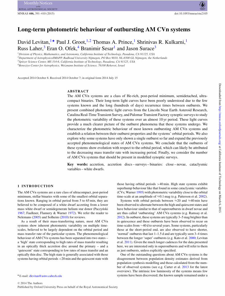
In Figs 1–5 we present outburst light curves of 15 systems with mul-tiple observed outbursts. Two systems known to outburst frequently,PTF1 J1919+4815 and KL Dra, are not presented here due to lackof data in the currently discussed surveys, but we refer the readerto Levitan et al. (2014) and Ramsay et al. (2010), respectively, fordetailed analysis of their light curves. We used the outburst criteriadetailed in Section 2.2 to identify outbursts in a quantitative fashion,and provide summary data of the outburst characteristics in Table 2.We provide more in-depth discussion on selected systems below.All outburst times are relative to the start of the light curve, whichis indicated in the respective figure.
3.1.1 CR Boo
CR Boo was found to have a 46.3 d outburst recurrence time byKato et al. (2000), hereafter K00. However, Kato et al. (2001),hereafter K01, reported that this was not constant and that CR Boohad switched to a 14.7 d recurrence time in 2001. More recent workby Honeycutt et al. (2013), hereafter H13, presents 20 yr of CR Boophotometry and also shows significant changes in its photometricbehaviour. The more than 9 yr of regular monitoring presented here
4 http://ptf.caltech.edu/
MNRAS 446, 391–410 (2015)
at California Institute of T
echnology on March 6, 2015
http://mnras.oxfordjournals.org/
Dow
nloaded from
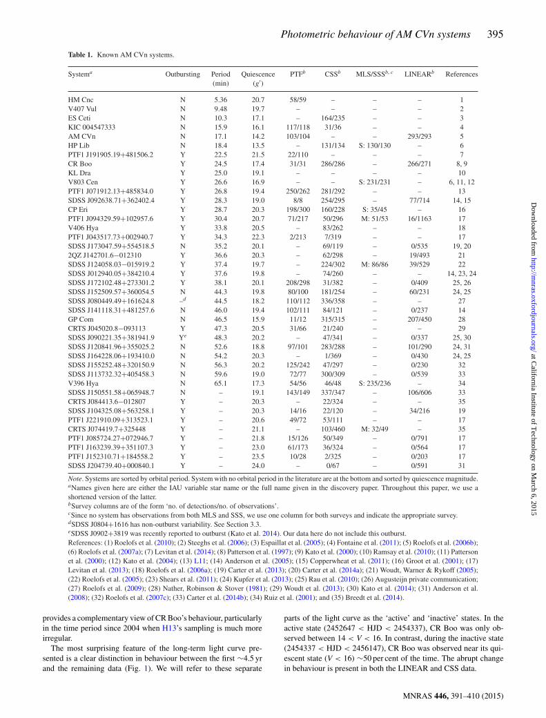
Photometric behaviour of AM CVn systems 395
Table 1. Known AM CVn systems.
Systema Outbursting Period Quiescence PTFb CSSb MLS/SSSb, c LINEARb References(min) (g′)
HM Cnc N 5.36 20.7 58/59 – – – 1V407 Vul N 9.48 19.7 – – – – 2ES Ceti N 10.3 17.1 – 164/235 – – 3KIC 004547333 N 15.9 16.1 117/118 31/36 – – 4AM CVn N 17.1 14.2 103/104 – – 293/293 5HP Lib N 18.4 13.5 – 131/134 S: 130/130 – 6PTF1 J191905.19+481506.2 Y 22.5 21.5 22/110 – – – 7CR Boo Y 24.5 17.4 31/31 286/286 – 266/271 8, 9KL Dra Y 25.0 19.1 – – – – 10V803 Cen Y 26.6 16.9 – – S: 231/231 – 6, 11, 12PTF1 J071912.13+485834.0 Y 26.8 19.4 250/262 281/292 – – 13SDSS J092638.71+362402.4 Y 28.3 19.0 8/8 254/295 – 77/714 14, 15CP Eri Y 28.7 20.3 198/300 160/228 S: 35/45 – 16PTF1 J094329.59+102957.6 Y 30.4 20.7 71/217 50/296 M: 51/53 16/1163 17V406 Hya Y 33.8 20.5 – 83/262 – – 18PTF1 J043517.73+002940.7 Y 34.3 22.3 2/213 7/319 – – 17SDSS J173047.59+554518.5 N 35.2 20.1 – 69/119 – 0/535 19, 202QZ J142701.6−012310 Y 36.6 20.3 – 62/298 – 19/493 21SDSS J124058.03−015919.2 Y 37.4 19.7 – 224/302 M: 86/86 39/529 22SDSS J012940.05+384210.4 Y 37.6 19.8 – 74/260 – – 14, 23, 24SDSS J172102.48+273301.2 Y 38.1 20.1 208/298 31/382 – 0/409 25, 26SDSS J152509.57+360054.5 N 44.3 19.8 80/100 181/254 – 60/231 24, 25SDSS J080449.49+161624.8 –d 44.5 18.2 110/112 336/358 – – 27SDSS J141118.31+481257.6 N 46.0 19.4 102/111 84/121 – 0/237 14GP Com N 46.5 15.9 11/12 315/315 – 207/450 28CRTS J045020.8−093113 Y 47.3 20.5 31/66 21/240 – – 29SDSS J090221.35+381941.9 Ye 48.3 20.2 – 47/341 – 0/337 25, 30SDSS J120841.96+355025.2 N 52.6 18.8 97/101 283/288 – 101/290 24, 31SDSS J164228.06+193410.0 N 54.2 20.3 – 1/369 – 0/430 24, 25SDSS J155252.48+320150.9 N 56.3 20.2 125/242 47/297 – 0/230 32SDSS J113732.32+405458.3 N 59.6 19.0 72/77 300/309 – 0/539 33V396 Hya N 65.1 17.3 54/56 46/48 S: 235/236 – 34SDSS J150551.58+065948.7 N – 19.1 143/149 337/347 – 106/606 33CRTS J084413.6−012807 Y – 20.3 – 22/324 – – 35SDSS J104325.08+563258.1 Y – 20.3 14/16 22/120 – 34/216 19PTF1 J221910.09+313523.1 Y – 20.6 49/72 53/111 – – 17CRTS J074419.7+325448 Y – 21.1 – 103/460 M: 32/49 – 35PTF1 J085724.27+072946.7 Y – 21.8 15/126 50/349 – 0/791 17PTF1 J163239.39+351107.3 Y – 23.0 61/173 36/324 – 0/564 17PTF1 J152310.71+184558.2 Y – 23.5 10/28 2/325 – 0/203 17SDSS J204739.40+000840.1 Y – 24.0 – 0/67 – 0/591 31
Note. Systems are sorted by orbital period. System with no orbital period in the literature are at the bottom and sorted by quiescence magnitude.aNames given here are either the IAU variable star name or the full name given in the discovery paper. Throughout this paper, we use ashortened version of the latter.bSurvey columns are of the form ‘no. of detections/no. of observations’.cSince no system has observations from both MLS and SSS, we use one column for both surveys and indicate the appropriate survey.dSDSS J0804+1616 has non-outburst variability. See Section 3.3.eSDSS J0902+3819 was recently reported to outburst (Kato et al. 2014). Our data here do not include this outburst.References: (1) Roelofs et al. (2010); (2) Steeghs et al. (2006); (3) Espaillat et al. (2005); (4) Fontaine et al. (2011); (5) Roelofs et al. (2006b);(6) Roelofs et al. (2007a); (7) Levitan et al. (2014); (8) Patterson et al. (1997); (9) Kato et al. (2000); (10) Ramsay et al. (2010); (11) Pattersonet al. (2000); (12) Kato et al. (2004); (13) L11; (14) Anderson et al. (2005); (15) Copperwheat et al. (2011); (16) Groot et al. (2001); (17)Levitan et al. (2013); (18) Roelofs et al. (2006a); (19) Carter et al. (2013); (20) Carter et al. (2014a); (21) Woudt, Warner & Rykoff (2005);(22) Roelofs et al. (2005); (23) Shears et al. (2011); (24) Kupfer et al. (2013); (25) Rau et al. (2010); (26) Augusteijn private communication;(27) Roelofs et al. (2009); (28) Nather, Robinson & Stover (1981); (29) Woudt et al. (2013); (30) Kato et al. (2014); (31) Anderson et al.(2008); (32) Roelofs et al. (2007c); (33) Carter et al. (2014b); (34) Ruiz et al. (2001); and (35) Breedt et al. (2014).
provides a complementary view of CR Boo’s behaviour, particularlyin the time period since 2004 when H13’s sampling is much moreirregular.
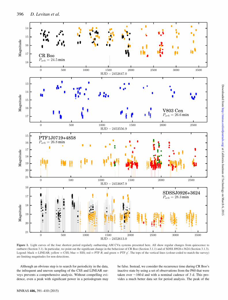
The most surprising feature of the long-term light curve pre-sented is a clear distinction in behaviour between the first ∼4.5 yrand the remaining data (Fig. 1). We will refer to these separate
parts of the light curve as the ‘active’ and ‘inactive’ states. In theactive state (2452647 < HJD < 2454337), CR Boo was only ob-served between 14 < V < 16. In contrast, during the inactive state(2454337 < HJD < 2456147), CR Boo was observed near its qui-escent state (V < 16) ∼50 per cent of the time. The abrupt changein behaviour is present in both the LINEAR and CSS data.
MNRAS 446, 391–410 (2015)
at California Institute of T
echnology on March 6, 2015
http://mnras.oxfordjournals.org/
Dow
nloaded from
396 D. Levitan et al.
Figure 1. Light curves of the four shortest period regularly outbursting AM CVn systems presented here. All show regular changes from quiescence tooutburst (Section 3.1). In particular, we point out the significant change in the behaviour of CR Boo (Section 3.1.1) and of SDSS J0926+3624 (Section 3.1.3).Legend: black = LINEAR; yellow = CSS; blue = SSS; red = PTF R; and green = PTF g′. The tops of the vertical lines (colour-coded to match the survey)are limiting magnitudes for non-detections.
Although an obvious step is to search for periodicity in the data,the infrequent and uneven sampling of the CSS and LINEAR sur-veys prevents a comprehensive analysis. Without compelling evi-dence, even a peak with significant power in a periodogram may
be false. Instead, we consider the recurrence time during CR Boo’sinactive state by using a set of observations from the P60 that weretaken over ∼160 d and with a nominal cadence of 3 d. This pro-vides a much better data set for period analysis. The peak of the
MNRAS 446, 391–410 (2015)
at California Institute of T
echnology on March 6, 2015
http://mnras.oxfordjournals.org/
Dow
nloaded from
Photometric behaviour of AM CVn systems 397
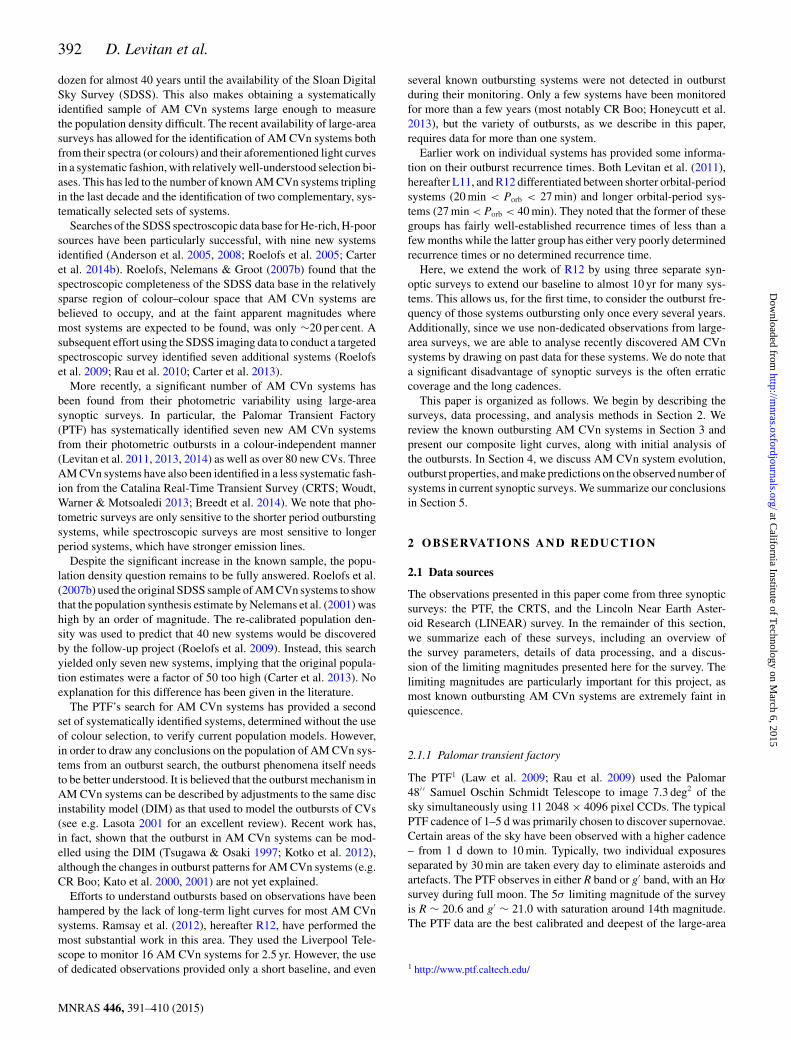
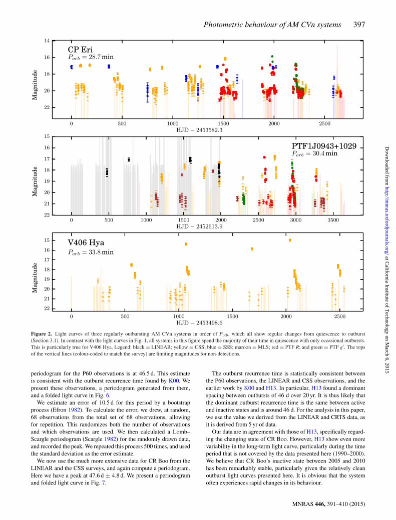
Figure 2. Light curves of three regularly outbursting AM CVn systems in order of Porb, which all show regular changes from quiescence to outburst(Section 3.1). In contrast with the light curves in Fig. 1, all systems in this figure spend the majority of their time in quiescence with only occasional outbursts.This is particularly true for V406 Hya. Legend: black = LINEAR; yellow = CSS; blue = SSS; maroon = MLS; red = PTF R; and green = PTF g′. The topsof the vertical lines (colour-coded to match the survey) are limiting magnitudes for non-detections.
periodogram for the P60 observations is at 46.5 d. This estimateis consistent with the outburst recurrence time found by K00. Wepresent these observations, a periodogram generated from them,and a folded light curve in Fig. 6.
We estimate an error of 10.5 d for this period by a bootstrapprocess (Efron 1982). To calculate the error, we drew, at random,68 observations from the total set of 68 observations, allowingfor repetition. This randomizes both the number of observationsand which observations are used. We then calculated a Lomb–Scargle periodogram (Scargle 1982) for the randomly drawn data,and recorded the peak. We repeated this process 500 times, and usedthe standard deviation as the error estimate.
We now use the much more extensive data for CR Boo from theLINEAR and the CSS surveys, and again compute a periodogram.Here we have a peak at 47.6 d ± 4.8 d. We present a periodogramand folded light curve in Fig. 7.
The outburst recurrence time is statistically consistent betweenthe P60 observations, the LINEAR and CSS observations, and theearlier work by K00 and H13. In particular, H13 found a dominantspacing between outbursts of 46 d over 20 yr. It is thus likely thatthe dominant outburst recurrence time is the same between activeand inactive states and is around 46 d. For the analysis in this paper,we use the value we derived from the LINEAR and CRTS data, asit is derived from 5 yr of data.
Our data are in agreement with those of H13, specifically regard-ing the changing state of CR Boo. However, H13 show even morevariability in the long-term light curve, particularly during the timeperiod that is not covered by the data presented here (1990–2000).We believe that CR Boo’s inactive state between 2005 and 2010has been remarkably stable, particularly given the relatively cleanoutburst light curves presented here. It is obvious that the systemoften experiences rapid changes in its behaviour.
MNRAS 446, 391–410 (2015)
at California Institute of T
echnology on March 6, 2015
http://mnras.oxfordjournals.org/
Dow
nloaded from
398 D. Levitan et al.
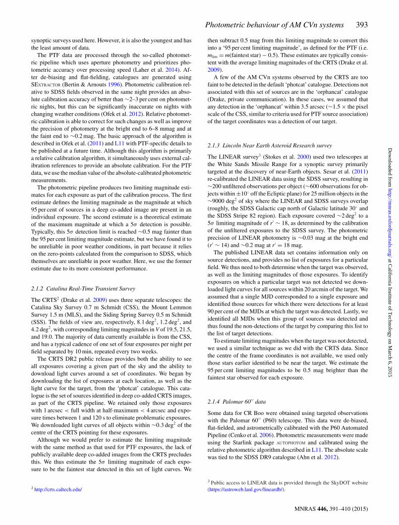
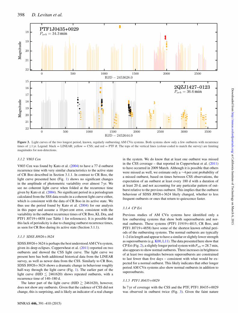
Figure 3. Light curves of the two longest period, known, regularly outbursting AM CVn systems. Both systems show only a few outbursts with recurrencetimes of ≥1 yr. Legend: black = LINEAR; yellow = CSS; and red = PTF R. The tops of the vertical lines (colour-coded to match the survey) are limitingmagnitudes for non-detections.
3.1.2 V803 Cen
V803 Cen was found by Kato et al. (2004) to have a 77 d outburstrecurrence time with very similar characteristics to the active stateof CR Boo described in Section 3.1.1. In contrast to CR Boo, thelight curve presented here (Fig. 1) shows no significant changesin the amplitude of photometric variability over almost 7 yr. Wesee no coherent light curve when folded at the recurrence timegiven by Kato et al. (2004). No significant period in a periodogramcalculated from the SSS data results in a coherent light curve either,which is consistent with the data of CR Boo in its active state. Wethus use the period found by Kato et al. (2004) for our analysisin this paper and assume a 10 per cent error, consistent with thevariability in the outburst recurrence times of CR Boo, KL Dra, andPTF1 J0719+4858 (see Table 1 for references). It is possible thatthis lack of periodicity is due to changing outburst recurrence times,as seen for CR Boo during its active state (Section 3.1.1).
3.1.3 SDSS J0926+3624
SDSS J0926+3624 is perhaps the best understood AM CVn system,given its deep eclipses. Copperwheat et al. (2011) reported on twooutbursts and showed the CSS light curve. The light curve wepresent here has both additional historical data from the LINEARsurvey, as well as newer data from the CSS. Similarly to CR Boo,SDSS J0926+3624 shows a dramatic change in behaviour roughlyhalf-way through the light curve (Fig. 1). The earlier part of thelight curve (HJD � 2461620) shows repeated outbursts, with arecurrence time of 140–180 d.
The latter part of the light curve (HJD � 2461620), however,does not show any outbursts. Given that the cadence of CSS did notchange, this is surprising, and is likely an indicator of a real change
in the system. We do know that at least one outburst was missedin the CSS coverage – that reported in Copperwheat et al. (2011)to have occurred in 2009 March. Although it is possible that otherswere missed as well, we estimate only a ∼4 per cent probability ofa missed outburst, based on times between CSS observations, theexpectation of an outburst at least every 180 d with a duration ofat least 20 d, and not accounting for any particular pattern of out-burst relative to the previous outburst. This implies that the outburstbehaviour of SDSS J0926+3624 likely changed, whether to lessfrequent outbursts or ones that return to quiescence faster.
3.1.4 CP Eri
Previous studies of AM CVn systems have identified only afew outbursting systems that show both superoutbursts and nor-mal outbursts. These systems (PTF1 J1919+4815, CR Boo, andPTF1 J0719+4858) have some of the shortest known orbital peri-ods of the outbursting systems. The normal outbursts are typically1–2 d in length and appear to have a similar or slightly lower strengthas superoutbursts (e.g. K00, L11). The data presented here show thatCP Eri (Fig. 2), a slightly longer period system with Porb = 28.7 min,also appears to show normal outbursts. Three increases in brightnessof at least two magnitudes between superoutbursts are constrainedto last fewer than five days – consistent with what would be ex-pected for a normal outburst. This likely indicates that other longerperiod AM CVn systems also show normal outbursts in addition tosuperoutbursts.
3.1.5 PTF1 J0435+0029
In 7 yr of coverage with the CSS and the PTF, PTF1 J0435+0029was observed in outburst twice (Fig. 3). Given the faint nature
MNRAS 446, 391–410 (2015)
at California Institute of T
echnology on March 6, 2015
http://mnras.oxfordjournals.org/
Dow
nloaded from
Photometric behaviour of AM CVn systems 399
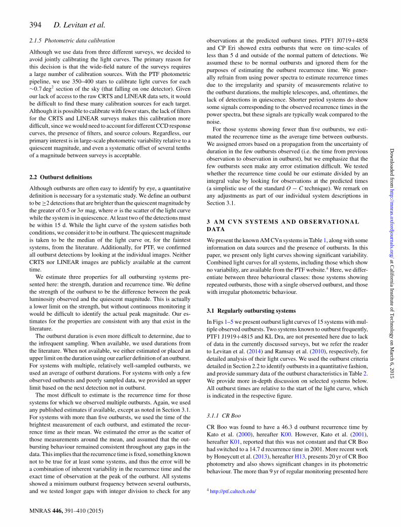
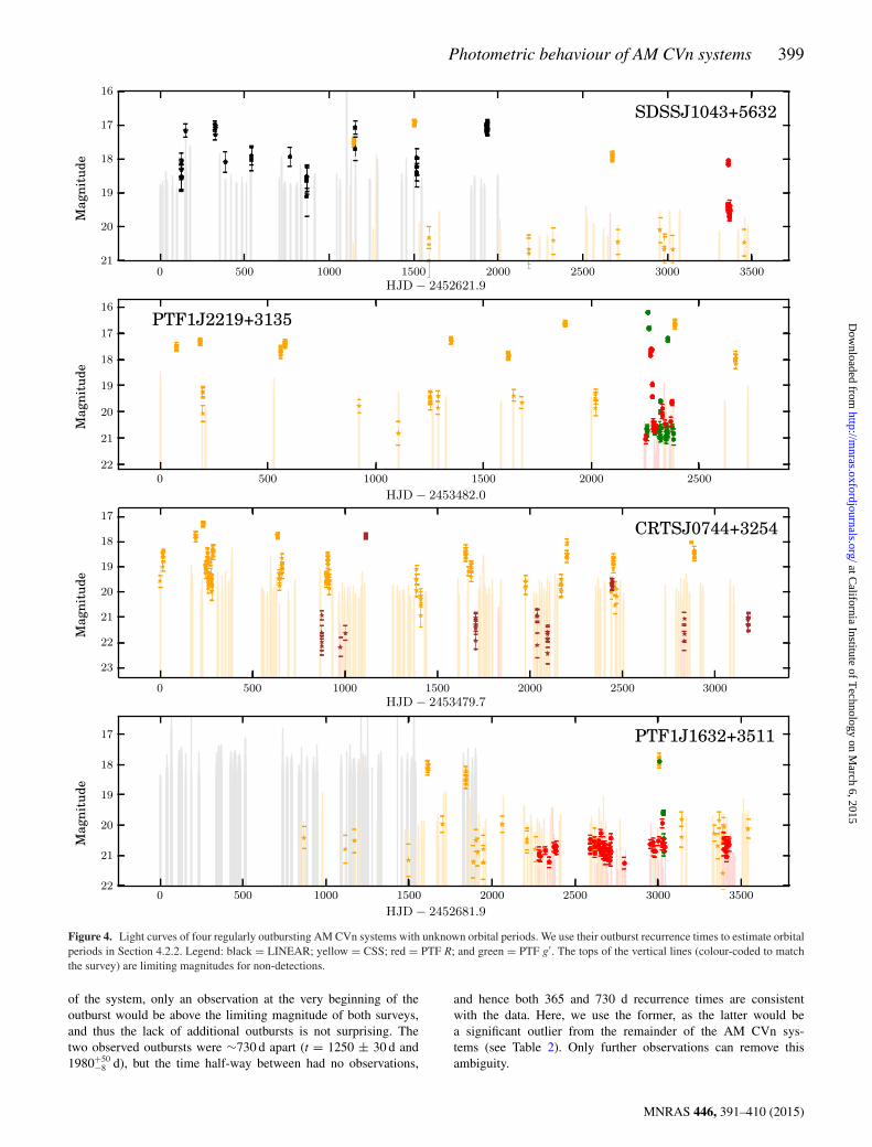
Figure 4. Light curves of four regularly outbursting AM CVn systems with unknown orbital periods. We use their outburst recurrence times to estimate orbitalperiods in Section 4.2.2. Legend: black = LINEAR; yellow = CSS; red = PTF R; and green = PTF g′. The tops of the vertical lines (colour-coded to matchthe survey) are limiting magnitudes for non-detections.
of the system, only an observation at the very beginning of theoutburst would be above the limiting magnitude of both surveys,and thus the lack of additional outbursts is not surprising. Thetwo observed outbursts were ∼730 d apart (t = 1250 ± 30 d and1980+50
−8 d), but the time half-way between had no observations,
and hence both 365 and 730 d recurrence times are consistentwith the data. Here, we use the former, as the latter would bea significant outlier from the remainder of the AM CVn sys-tems (see Table 2). Only further observations can remove thisambiguity.
MNRAS 446, 391–410 (2015)
at California Institute of T
echnology on March 6, 2015
http://mnras.oxfordjournals.org/
Dow
nloaded from
400 D. Levitan et al.
Figure 5. Light curves of two regularly outbursting AM CVn systems with unknown orbital periods and extremely long outburst recurrence times. These arediscussed in Section 3.1.7. Legend: black = LINEAR; yellow = CSS; red = PTF R; and green = PTF g′. The tops of the vertical lines (colour-coded to matchthe survey) are limiting magnitudes for non-detections.
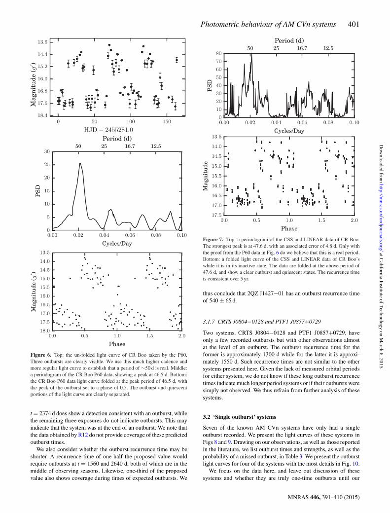
Table 2. Outburst properties of recurring outburst systems with known orbital periods.
System orbital No. of outbursts Observation Recurrence Duration Strengthper. (min) pbserved span (d) time (d) (d) (mag)
PTF1 J1919+4815a 22.5 – – 36.8 ± 0.4 ∼13 3CR Boob 24.5 –c 3445 47.6 ± 4.8 ∼24 3.3KL Draa 25.0 – – 44–65 ∼15 4.2V803 Cena 26.6 –c 2545 77 – 4.6PTF1 J0719+4858a 26.8 23 2581 65–80 ∼18 3.5SDSS J0926+3624 28.3 9 3462 160 ± 20 ∼20 2.4CP Eri 28.7 13 2691 108 ± 13 ∼20 4.2PTF1 J0943+1029 30.4 10 3645 110 ± 14 <30 4.1V406 Hya 33.8 5 2540 280 ± 50 <100 5.9PTF1 J0435+0029 34.3 2 2629 365 ± 60 <60 5.12QZ J1427−0123 36.6 3 3455 540 ± 60 <50 4.3
Note. Definitions of the properties shown here are in Section 2.2.aProperties presented here (except observation details) are from the literature. See Table 1 for references.bThe reported data are from only the second half of CR Boo observations presented in this paper (seeSection 3.1.1).cWe do not count the number of outbursts due to the complicated and rapidly changing nature of the lightcurve.
3.1.6 2QZ J1427−01
We find three outbursts for 2QZ J1427−01 (Fig. 3), with peakmagnitudes at t = 760+40
−50 , 1240+30−20, and 1830+10
−30 d. We constrain theduration of the outbursts to <50 d, based on the second outburst. Weprovide estimates for the remaining two outbursts using this outburstduration to obtain a lower bound on their times of peak luminosity,since both outbursts occurred before the start of an observing season.The mean difference between these peaks is 540 ± 65 d, with theerror derived based on the errors of each outburst peak. We note that
this is roughly consistent with the 10–20 per cent change in outburstrecurrence time observed in shorter period systems.
These outbursts occur over a period of ∼1000 d, while we havedata over a time span of >3500 d. We thus expect additional out-bursts at t ≈ 210, 2370, 2910, and 3450 d. The first falls betweenobserving seasons, while the third and fourth are just before andafter an observing season, respectively. Given the associated error,it is highly likely that no outburst would have been seen. Thereare observations at t = 2354, 2374, and 2401 d, roughly coincidentwith when we would expect an outburst. One of the exposures on
MNRAS 446, 391–410 (2015)
at California Institute of T
echnology on March 6, 2015
http://mnras.oxfordjournals.org/
Dow
nloaded from
Photometric behaviour of AM CVn systems 401
Figure 6. Top: the un-folded light curve of CR Boo taken by the P60.Three outbursts are clearly visible. We use this much higher cadence andmore regular light curve to establish that a period of ∼50 d is real. Middle:a periodogram of the CR Boo P60 data, showing a peak at 46.5 d. Bottom:the CR Boo P60 data light curve folded at the peak period of 46.5 d, withthe peak of the outburst set to a phase of 0.5. The outburst and quiescentportions of the light curve are clearly separated.
t = 2374 d does show a detection consistent with an outburst, whilethe remaining three exposures do not indicate outbursts. This mayindicate that the system was at the end of an outburst. We note thatthe data obtained by R12 do not provide coverage of these predictedoutburst times.
We also consider whether the outburst recurrence time may beshorter. A recurrence time of one-half the proposed value wouldrequire outbursts at t = 1560 and 2640 d, both of which are in themiddle of observing seasons. Likewise, one-third of the proposedvalue also shows coverage during times of expected outbursts. We
Figure 7. Top: a periodogram of the CSS and LINEAR data of CR Boo.The strongest peak is at 47.6 d, with an associated error of 4.8 d. Only withthe proof from the P60 data in Fig. 6 do we believe that this is a real period.Bottom: a folded light curve of the CSS and LINEAR data of CR Boo’swhile it is in its inactive state. The data are folded at the above period of47.6 d, and show a clear outburst and quiescent states. The recurrence timeis consistent over 5 yr.
thus conclude that 2QZ J1427−01 has an outburst recurrence timeof 540 ± 65 d.
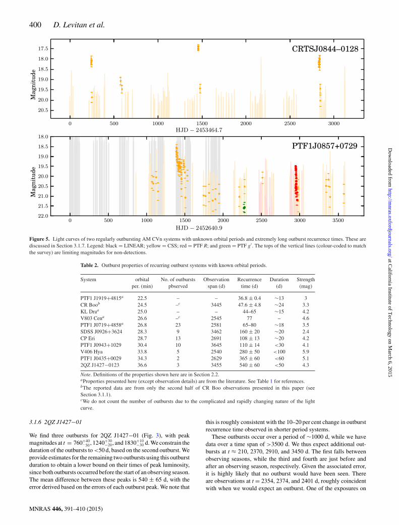
3.1.7 CRTS J0804−0128 and PTF1 J0857+0729
Two systems, CRTS J0804−0128 and PTF1 J0857+0729, haveonly a few recorded outbursts but with other observations almostat the level of an outburst. The outburst recurrence time for theformer is approximately 1300 d while for the latter it is approxi-mately 1550 d. Such recurrence times are not similar to the othersystems presented here. Given the lack of measured orbital periodsfor either system, we do not know if these long outburst recurrencetimes indicate much longer period systems or if their outbursts weresimply not observed. We thus refrain from further analysis of thesesystems.
3.2 ‘Single outburst’ systems
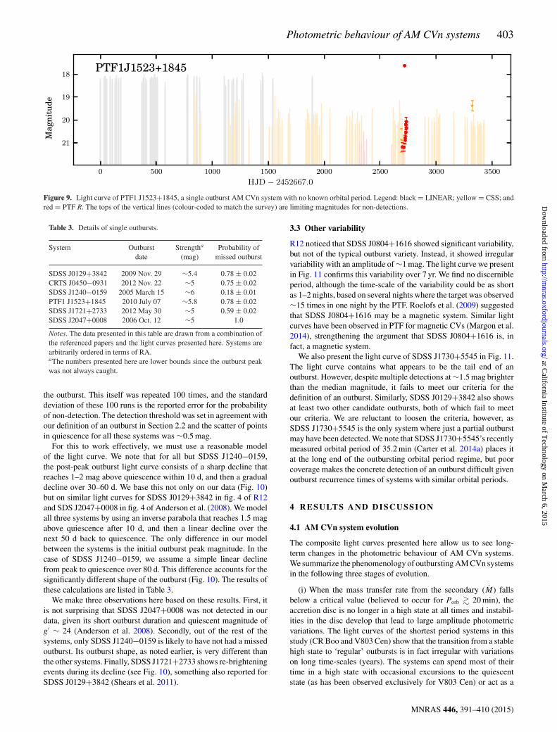
Seven of the known AM CVn systems have only had a singleoutburst recorded. We present the light curves of these systems inFigs 8 and 9. Drawing on our observations, as well as those reportedin the literature, we list outburst times and strengths, as well as theprobability of a missed outburst, in Table 3. We present the outburstlight curves for four of the systems with the most details in Fig. 10.
We focus on the data here, and leave out discussion of thesesystems and whether they are truly one-time outbursts until our
MNRAS 446, 391–410 (2015)
at California Institute of T
echnology on March 6, 2015
http://mnras.oxfordjournals.org/
Dow
nloaded from
402 D. Levitan et al.
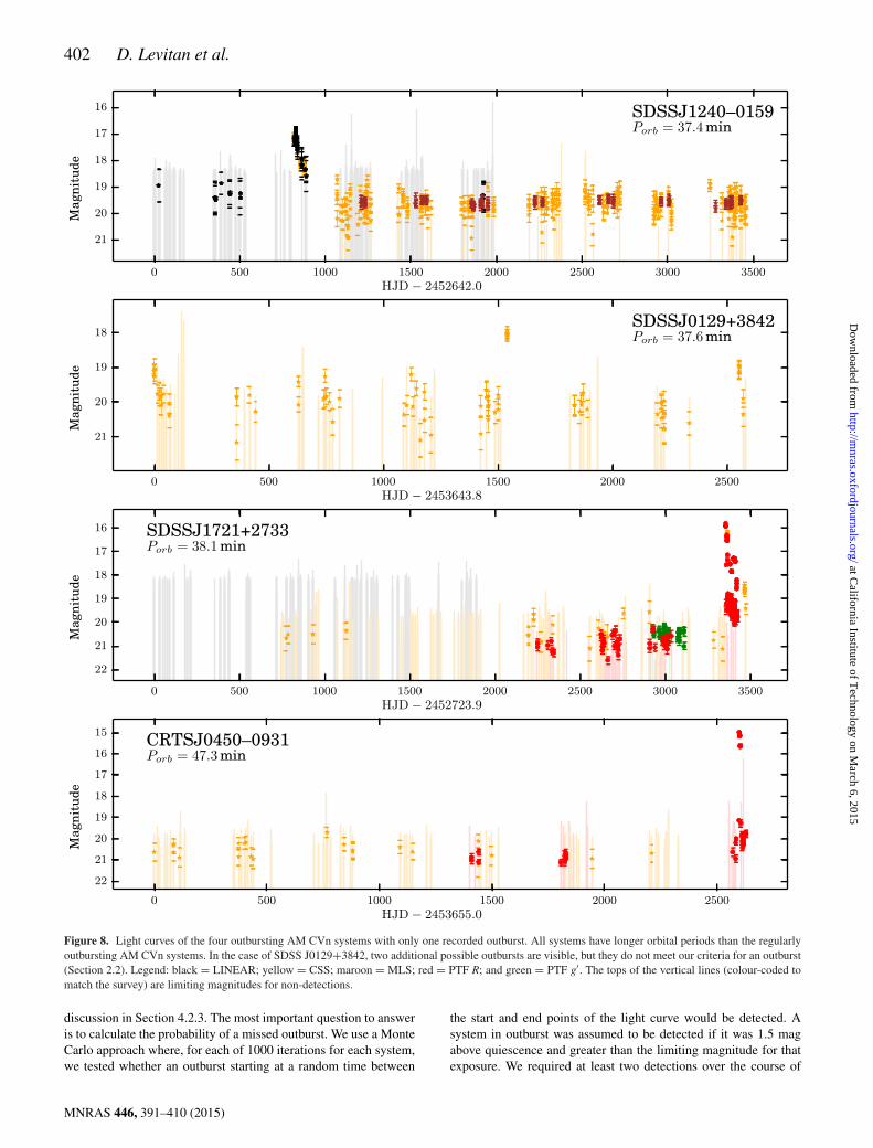
Figure 8. Light curves of the four outbursting AM CVn systems with only one recorded outburst. All systems have longer orbital periods than the regularlyoutbursting AM CVn systems. In the case of SDSS J0129+3842, two additional possible outbursts are visible, but they do not meet our criteria for an outburst(Section 2.2). Legend: black = LINEAR; yellow = CSS; maroon = MLS; red = PTF R; and green = PTF g′. The tops of the vertical lines (colour-coded tomatch the survey) are limiting magnitudes for non-detections.
discussion in Section 4.2.3. The most important question to answeris to calculate the probability of a missed outburst. We use a MonteCarlo approach where, for each of 1000 iterations for each system,we tested whether an outburst starting at a random time between
the start and end points of the light curve would be detected. Asystem in outburst was assumed to be detected if it was 1.5 magabove quiescence and greater than the limiting magnitude for thatexposure. We required at least two detections over the course of
MNRAS 446, 391–410 (2015)
at California Institute of T
echnology on March 6, 2015
http://mnras.oxfordjournals.org/
Dow
nloaded from
Photometric behaviour of AM CVn systems 403
Figure 9. Light curve of PTF1 J1523+1845, a single outburst AM CVn system with no known orbital period. Legend: black = LINEAR; yellow = CSS; andred = PTF R. The tops of the vertical lines (colour-coded to match the survey) are limiting magnitudes for non-detections.
Table 3. Details of single outbursts.
System Outburst Strengtha Probability ofdate (mag) missed outburst
SDSS J0129+3842 2009 Nov. 29 ∼5.4 0.78 ± 0.02CRTS J0450−0931 2012 Nov. 22 ∼5 0.75 ± 0.02SDSS J1240−0159 2005 March 15 ∼6 0.18 ± 0.01PTF1 J1523+1845 2010 July 07 ∼5.8 0.78 ± 0.02SDSS J1721+2733 2012 May 30 ∼5 0.59 ± 0.02SDSS J2047+0008 2006 Oct. 12 ∼5 1.0
Notes. The data presented in this table are drawn from a combination ofthe referenced papers and the light curves presented here. Systems arearbitrarily ordered in terms of RA.aThe numbers presented here are lower bounds since the outburst peakwas not always caught.
the outburst. This itself was repeated 100 times, and the standarddeviation of these 100 runs is the reported error for the probabilityof non-detection. The detection threshold was set in agreement withour definition of an outburst in Section 2.2 and the scatter of pointsin quiescence for all these systems was ∼0.5 mag.
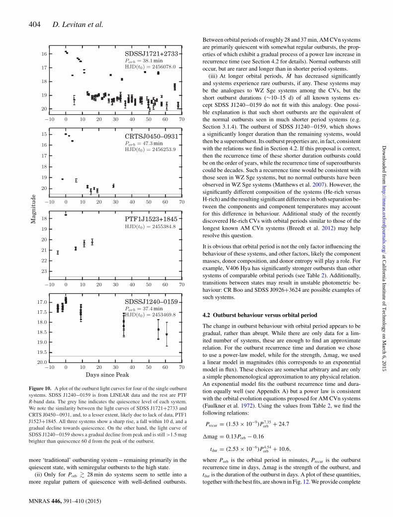
For this to work effectively, we must use a reasonable modelof the light curve. We note that for all but SDSS J1240−0159,the post-peak outburst light curve consists of a sharp decline thatreaches 1–2 mag above quiescence within 10 d, and then a gradualdecline over 30–60 d. We base this not only on our data (Fig. 10)but on similar light curves for SDSS J0129+3842 in fig. 4 of R12and SDS J2047+0008 in fig. 4 of Anderson et al. (2008). We modelall three systems by using an inverse parabola that reaches 1.5 magabove quiescence after 10 d, and then a linear decline over thenext 50 d back to quiescence. The only difference in our modelbetween the systems is the initial outburst peak magnitude. In thecase of SDSS J1240−0159, we assume a simple linear declinefrom peak to quiescence over 80 d. This difference accounts for thesignificantly different shape of the outburst (Fig. 10). The results ofthese calculations are listed in Table 3.
We make three observations here based on these results. First, itis not surprising that SDSS J2047+0008 was not detected in ourdata, given its short outburst duration and quiescent magnitude ofg′ ∼ 24 (Anderson et al. 2008). Secondly, out of the rest of thesystems, only SDSS J1240−0159 is likely to have not had a missedoutburst. Its outburst shape, as noted earlier, is very different thanthe other systems. Finally, SDSS J1721+2733 shows re-brighteningevents during its decline (see Fig. 10), something also reported forSDSS J0129+3842 (Shears et al. 2011).
3.3 Other variability
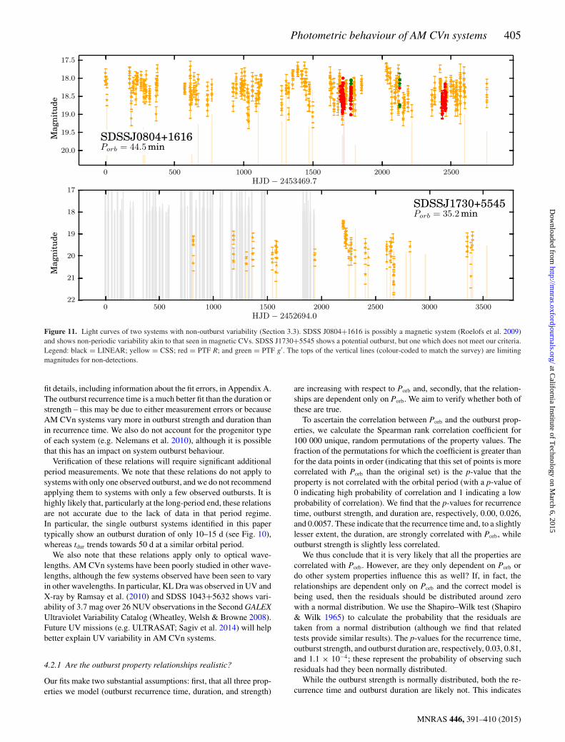
R12 noticed that SDSS J0804+1616 showed significant variability,but not of the typical outburst variety. Instead, it showed irregularvariability with an amplitude of ∼1 mag. The light curve we presentin Fig. 11 confirms this variability over 7 yr. We find no discernibleperiod, although the time-scale of the variability could be as shortas 1–2 nights, based on several nights where the target was observed∼15 times in one night by the PTF. Roelofs et al. (2009) suggestedthat SDSS J0804+1616 may be a magnetic system. Similar lightcurves have been observed in PTF for magnetic CVs (Margon et al.2014), strengthening the argument that SDSS J0804+1616 is, infact, a magnetic system.
We also present the light curve of SDSS J1730+5545 in Fig. 11.The light curve contains what appears to be the tail end of anoutburst. However, despite multiple detections at ∼1.5 mag brighterthan the median magnitude, it fails to meet our criteria for thedefinition of an outburst. Similarly, SDSS J0129+3842 also showsat least two other candidate outbursts, both of which fail to meetour criteria. We are reluctant to loosen the criteria, however, asSDSS J1730+5545 is the only system where just a partial outburstmay have been detected. We note that SDSS J1730+5545’s recentlymeasured orbital period of 35.2 min (Carter et al. 2014a) places itat the long end of the outbursting orbital period regime, but poorcoverage makes the concrete detection of an outburst difficult givenoutburst recurrence times of systems with similar orbital periods.
4 R ESULTS AND DI SCUSSI ON
4.1 AM CVn system evolution
The composite light curves presented here allow us to see long-term changes in the photometric behaviour of AM CVn systems.We summarize the phenomenology of outbursting AM CVn systemsin the following three stages of evolution.
(i) When the mass transfer rate from the secondary (M) fallsbelow a critical value (believed to occur for Porb � 20 min), theaccretion disc is no longer in a high state at all times and instabil-ities in the disc develop that lead to large amplitude photometricvariations. The light curves of the shortest period systems in thisstudy (CR Boo and V803 Cen) show that the transition from a stablehigh state to ‘regular’ outbursts is in fact irregular with variationson long time-scales (years). The systems can spend most of theirtime in a high state with occasional excursions to the quiescentstate (as has been observed exclusively for V803 Cen) or act as a
MNRAS 446, 391–410 (2015)
at California Institute of T
echnology on March 6, 2015
http://mnras.oxfordjournals.org/
Dow
nloaded from
404 D. Levitan et al.
Figure 10. A plot of the outburst light curves for four of the single outburstsystems. SDSS J1240−0159 is from LINEAR data and the rest are PTFR-band data. The grey line indicates the quiescence level of each system.We note the similarity between the light curves of SDSS J1721+2733 andCRTS J0450−0931, and, to a lesser extent, likely due to lack of data, PTF1J1523+1845. All three systems show a sharp rise, a fall within 10 d, and agradual decline towards quiescence. On the other hand, the light curve ofSDSS J1240−0159 shows a gradual decline from peak and is still >1.5 magbrighter than quiescence 60 d from the peak of the outburst.
more ‘traditional’ outbursting system – remaining primarily in thequiescent state, with semiregular outbursts to the high state.
(ii) Only for Porb � 28 min do systems seem to settle into amore regular pattern of quiescence with well-defined outbursts.
Between orbital periods of roughly 28 and 37 min, AM CVn systemsare primarily quiescent with somewhat regular outbursts, the prop-erties of which exhibit a gradual process of a power law increase inrecurrence time (see Section 4.2 for details). Normal outbursts stilloccur, but are rarer and longer than in shorter period systems.
(iii) At longer orbital periods, M has decreased significantlyand systems experience rare outbursts, if any. These systems maybe the analogues to WZ Sge systems among the CVs, but theshort outburst durations (∼10–15 d) of all known systems ex-cept SDSS J1240−0159 do not fit with this analogy. One possi-ble explanation is that such short outbursts are the equivalent ofthe normal outbursts seen in much shorter period systems (e.g.Section 3.1.4). The outburst of SDSS J1240−0159, which showsa significantly longer duration than the remaining systems, wouldthen be a superoutburst. Its outburst properties are, in fact, consistentwith the relations we find in Section 4.2. If this proposal is correct,then the recurrence time of these shorter duration outbursts couldbe on the order of years, while the recurrence time of superoutburstscould be decades. Such a recurrence time would be consistent withthose seen in WZ Sge systems, but no normal outbursts have beenobserved in WZ Sge systems (Matthews et al. 2007). However, thesignificantly different composition of the systems (He-rich versusH-rich) and the resulting significant difference in both separation be-tween the components and component temperatures may accountfor this difference in behaviour. Additional study of the recentlydiscovered He-rich CVs with orbital periods similar to those of thelongest known AM CVn systems (Breedt et al. 2012) may helpresolve this question.
It is obvious that orbital period is not the only factor influencing thebehaviour of these systems, and other factors, likely the componentmasses, donor composition, and donor entropy will play a role. Forexample, V406 Hya has significantly stronger outbursts than othersystems of comparable orbital periods (see Table 2). Additionally,transitions between states may result in unstable photometric be-haviour: CR Boo and SDSS J0926+3624 are possible examples ofsuch systems.
4.2 Outburst behaviour versus orbital period
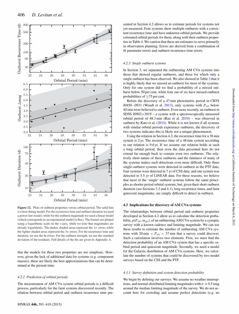
The change in outburst behaviour with orbital period appears to begradual, rather than abrupt. While there are only data for a lim-ited number of systems, these are enough to find an approximaterelation. For the outburst recurrence time and duration we choseto use a power-law model, while for the strength, �mag, we useda linear model in magnitudes (this corresponds to an exponentialmodel in flux). These choices are somewhat arbitrary and are onlya simple phenomenological approximation to any physical relation.An exponential model fits the outburst recurrence time and dura-tion equally well (see Appendix A) but a power law is consistentwith the orbital evolution equations proposed for AM CVn systems(Faulkner et al. 1972). Using the values from Table 2, we find thefollowing relations:
Precur = (1.53 × 10⁻⁹)P 7.35orb + 24.7
�mag = 0.13Porb − 0.16
tdur = (2.53 × 10⁻⁶)P 4.54orb + 10.6,
where Porb is the orbital period in minutes, Precur is the outburstrecurrence time in days, �mag is the strength of the outburst, andtdur is the duration of the outburst in days. A plot of these quantities,together with the best fits, are shown in Fig. 12. We provide complete
MNRAS 446, 391–410 (2015)
at California Institute of T
echnology on March 6, 2015
http://mnras.oxfordjournals.org/
Dow
nloaded from
Photometric behaviour of AM CVn systems 405
Figure 11. Light curves of two systems with non-outburst variability (Section 3.3). SDSS J0804+1616 is possibly a magnetic system (Roelofs et al. 2009)and shows non-periodic variability akin to that seen in magnetic CVs. SDSS J1730+5545 shows a potential outburst, but one which does not meet our criteria.Legend: black = LINEAR; yellow = CSS; red = PTF R; and green = PTF g′. The tops of the vertical lines (colour-coded to match the survey) are limitingmagnitudes for non-detections.
fit details, including information about the fit errors, in Appendix A.The outburst recurrence time is a much better fit than the duration orstrength – this may be due to either measurement errors or becauseAM CVn systems vary more in outburst strength and duration thanin recurrence time. We also do not account for the progenitor typeof each system (e.g. Nelemans et al. 2010), although it is possiblethat this has an impact on system outburst behaviour.
Verification of these relations will require significant additionalperiod measurements. We note that these relations do not apply tosystems with only one observed outburst, and we do not recommendapplying them to systems with only a few observed outbursts. It ishighly likely that, particularly at the long-period end, these relationsare not accurate due to the lack of data in that period regime.In particular, the single outburst systems identified in this papertypically show an outburst duration of only 10–15 d (see Fig. 10),whereas tdur trends towards 50 d at a similar orbital period.
We also note that these relations apply only to optical wave-lengths. AM CVn systems have been poorly studied in other wave-lengths, although the few systems observed have been seen to varyin other wavelengths. In particular, KL Dra was observed in UV andX-ray by Ramsay et al. (2010) and SDSS 1043+5632 shows vari-ability of 3.7 mag over 26 NUV observations in the Second GALEXUltraviolet Variability Catalog (Wheatley, Welsh & Browne 2008).Future UV missions (e.g. ULTRASAT; Sagiv et al. 2014) will helpbetter explain UV variability in AM CVn systems.
4.2.1 Are the outburst property relationships realistic?
Our fits make two substantial assumptions: first, that all three prop-erties we model (outburst recurrence time, duration, and strength)
are increasing with respect to Porb and, secondly, that the relation-ships are dependent only on Porb. We aim to verify whether both ofthese are true.
To ascertain the correlation between Porb and the outburst prop-erties, we calculate the Spearman rank correlation coefficient for100 000 unique, random permutations of the property values. Thefraction of the permutations for which the coefficient is greater thanfor the data points in order (indicating that this set of points is morecorrelated with Porb than the original set) is the p-value that theproperty is not correlated with the orbital period (with a p-value of0 indicating high probability of correlation and 1 indicating a lowprobability of correlation). We find that the p-values for recurrencetime, outburst strength, and duration are, respectively, 0.00, 0.026,and 0.0057. These indicate that the recurrence time and, to a slightlylesser extent, the duration, are strongly correlated with Porb, whileoutburst strength is slightly less correlated.
We thus conclude that it is very likely that all the properties arecorrelated with Porb. However, are they only dependent on Porb ordo other system properties influence this as well? If, in fact, therelationships are dependent only on Porb and the correct model isbeing used, then the residuals should be distributed around zerowith a normal distribution. We use the Shapiro–Wilk test (Shapiro& Wilk 1965) to calculate the probability that the residuals aretaken from a normal distribution (although we find that relatedtests provide similar results). The p-values for the recurrence time,outburst strength, and outburst duration are, respectively, 0.03, 0.81,and 1.1 × 10⁻⁴; these represent the probability of observing suchresiduals had they been normally distributed.
While the outburst strength is normally distributed, both the re-currence time and outburst duration are likely not. This indicates
MNRAS 446, 391–410 (2015)
at California Institute of T
echnology on March 6, 2015
http://mnras.oxfordjournals.org/
Dow
nloaded from
406 D. Levitan et al.
Figure 12. Plots of outburst properties versus orbital period. The solid lineis a best-fitting model. For the recurrence time and outburst duration we useda power-law model, while for the outburst magnitude we used a linear model(which corresponds to an exponential model in flux). The former are plottedusing a logarithmic scale on the y-axis, while we note that magnitudes arealready logarithmic. The darker shaded areas represent the 1σ errors whilethe lighter shaded areas represent the 3σ errors. For the recurrence time andduration, we use the fit errors. For the outburst strength, we use the standarddeviation of the residuals. Full details of the fits are given in Appendix A.
that the models for these two properties are too simplistic. How-ever, given the lack of additional data for systems (e.g. componentmasses), these are likely the best approximations that can be deter-mined at the present time.
4.2.2 Prediction of orbital periods
The measurement of AM CVn system orbital periods is a difficultprocess, particularly for the faint systems discovered recently. Therelation between orbital period and outburst recurrence time pre-
sented in Section 4.2 allows us to estimate periods for systems notyet measured. Four systems show multiple outbursts with a consis-tent recurrence time and have unknown orbital periods. We provideestimated orbital periods for them, along with their outburst proper-ties in Table 4. We caution that these are estimates to serve primarilyin observation planning. Errors are derived from a combination offit parameter errors and outburst recurrence time errors.
4.2.3 Single outburst systems
In Section 3, we separated the outbursting AM CVn systems intothose that showed regular outbursts, and those for which only asingle outburst has been observed. We also showed in Table 3 that itis highly likely that we missed an outburst for most of the systems.Only for one system did we find a probability of a missed out-burst below 50 per cent, while four out of six have missed-outburstprobabilities of ≥75 per cent.
Before the discovery of a 47 min photometric period in CRTSJ0450−0931 (Woudt et al. 2013), only systems with Porb below40 min were believed to outburst. Even more recently, an outburst inSDSS J0902+3819 – a system with a spectroscopically measuredorbital period of 48.3 min (Rau et al. 2010) – was observed inoutburst by Kato et al. (2014). While it is not known if all systemswith similar orbital periods experience outbursts, the discovery oftwo systems indicates this is likely not a unique phenomenon.
Using the relation in Section 4.2, the recurrence time for a 38 minsystem is 2 yr. The recurrence time of a 48 min system accordingto our relation is 9.6 yr. If we assume our relation holds at sucha long orbital period, then even the data presented here do notextend far enough back to contain even two outbursts. The rela-tively short nature of these outbursts and the faintness of many ofthe systems makes such detections even more difficult. Only threesingle-outburst systems were detected in outburst in the PTF data,four systems were detected in 7 yr of CSS data, and one system wasdetected in 5.5 yr of LINEAR data. For these reasons, we believethat most of the ‘single’ outburst systems follow the same princi-ples as shorter period orbital systems, but, given their short outburstduration (see Sections 3.2 and 4.1), long recurrence times, and faintquiescent magnitudes, are simply difficult to detect in outburst.
4.3 Implications for discovery of AM CVn systems
The relationships between orbital period and outburst propertiesdeveloped in Section 4.2 allow us to calculate the detection proba-bility, p(Porb, mqui), of an outbursting AM CVn system by a synopticsurvey with a known cadence and limiting magnitude. We can usethese results to estimate the number of outbursting AM CVn sys-tems with 20 min < Porb < 37 min that a survey could discover.Such a calculation involves two elements. First, we must find thedetection probability of an AM CVn system that has a specific or-bital period and quiescent magnitude. Secondly, we need a modelfor the Galactic distribution of AM CVn systems. Here, we calcu-late the number of systems that could be discovered by two modelsurveys based on the CSS and the PTF.
4.3.1 Survey definition and system detection probability
We begin by defining our surveys. We assume no weather interrup-tions, and normal-distributed limiting magnitudes with σ = 0.5 magaround the median limiting magnitude of the survey. We do not ac-count here for crowding and assume perfect detections (e.g. no
MNRAS 446, 391–410 (2015)
at California Institute of T
echnology on March 6, 2015
http://mnras.oxfordjournals.org/
Dow
nloaded from
Photometric behaviour of AM CVn systems 407
Table 4. Outburst properties of recurring outburst systems with unknown orbital periods.
System No. of outbursts Observation Recurrence Duration Strength Est. orbitalobserved span (d) time (d) (d) (mag) Per. (min)
PTF1 J2219+3135 9 2726 64 ± 5 <26 4.4 26.1 ± 0.74SDSS 1043+5632 9 3477 99 ± 12 <55 3.4 28.5 ± 0.92PTF1 J1632+3511 3 3541 230 ± 35 <80 5.2 32.7 ± 1.1CRTS J0744+3254 12 3100 239 ± 36 <65 3.8 32.9 ± 1.1
Notes. Definitions of the properties shown here are in Section 2.2. The estimated orbital periods are based onoutburst properties and their calculation and accuracy are described in Section 4.2.2. Errors are derived from acombination of the outburst recurrence time error and the fit error. The outburst duration times for all of thesesystems are upper bounds due to lack of data to find a better estimate.
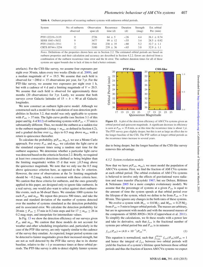
artefacts). For the CSS-like survey, we assume four exposures pernight over 30 min, taken every two weeks (Drake et al. 2009), anda median magnitude of V = 19.5. We assume that each field isobserved for ∼200 d = 15 observations per year, for 7 yr. For thePTF-like survey, we assume two exposures per night over 1 h,but with a cadence of 4 d and a limiting magnitude of V = 20.5.We assume that each field is observed for approximately threemonths (20 observations) for 3 yr. Lastly, we assume that bothsurveys cover Galactic latitudes of 15 < b < 90 at all Galacticlongitudes.
We now construct an outburst light-curve model. Although weconstructed such a model for the calculation of non-detection prob-abilities in Section 3.2, that model was only applicable to systemswith Porb > 37 min. The light-curve profile (see Section 3.1 of thispaper and fig. 4 of R12) of outbursting systems with Porb < 37 min issubstantially different. Thus, we model the outburst as a sudden riseto the outburst magnitude (�mag + mqui, as defined in Section 4.2),and a gradual decline over tdur days to 0.5 mag above mqui, with areturn to quiescence thereafter.
To calculate the probability, p(Porb, mqui), we use a Monte Carloapproach. For every Porb and mqui, we calculate the light curve atthe simulated exposure times using a random start time for theoutburst sequence. We determine whether a particular light curvewas detected based on the criteria in Section 2.2. Briefly, we requiredat least two consecutive detections (defined as being brighter thanthe limiting magnitude) within 15 d that were ≥0.5 mag abovethe quiescence magnitude. We note that we only use the 0.5 magabove quiescence criterion here, as opposed to the 3σ criterion.However, the error of observations at the 5σ limiting magnitudeshould be ∼0.2 mag, which is consistent with these criteria here.We caution that these criteria for outbursts, and the ones generallyapplied in this paper, are designed only to ignore fake outbursts. Ina real survey, one would also want to select against short outburst-like events, such as M-dwarf flares. We simulate 1000 systems foreach Porb and mqui. We repeat this process 500 times, and take themean and standard deviation of the number of systems detectedover the number of systems simulated as the detection probabilityand its associated error. We calculate the detection probability for20 min ≤ Porb ≤ 37 min in 0.2 min steps and for 17 ≤ mqui ≤ 26 in0.2 mag steps, and interpolate for intermediate values.
In Fig. 13 we show the detection efficiency of our surveys givenPorb and mqui. We caution that these models do not account forweather and other scheduling irregularities and, particularly in thecase of the PTF-like survey, are only vaguely similar to the cadenceof the survey they emulate. As expected, longer period systems canbe detected to fainter magnitudes given their increased strength, butare not as well detected by the PTF-like survey due to its shorterbaseline, relative to the >1 yr recurrence times at these orbital pe-riods. The PTF-like survey is able to detect slightly fainter systems
Figure 13. A plot of the detection efficiency of AM CVn systems given anorbital period and quiescent magnitude. A significant decrease in efficiencyis seen at Porb = 35.8 min, as at this time the recurrence time is about 1 yr.The PTF survey goes slightly deeper, but this is not as large an effect due tothe longer baseline of the CSS. The PTF suffers at longer orbital periods asthe recurrence times increase to several years.
due to being deeper, but the longer baseline of the CSS-like surveyremoves this advantage.
4.3.2 System evolution models
Now that we have p(Porb, mqui), we must model the population ofAM CVn systems. First, we find the fraction of AM CVn systemsat each orbital period. The orbital evolution of AM CVn systemsis believed to involve only the effects of gravitational wave radia-tion and mass transfer (Paczynski 1967; but see Deloye, Bildsten& Nelemans 2005 for a more complex evolutionary model). Weassume that the percentage of systems at a given Porb is equal tothe amount of time the system spends at that orbital period overthe lifespan of the system, which we define to be from Porb = 5 to80 min. This ignores any changes in the birth rates of these systems.
We evolve a system with Macc = 0.6 M and Mdon = 0.25 Mfrom Porb = 5 min to longer orbital periods. The masses are arbitrary,but are in agreement with models and with the measured masses ofthe components of SDSS J0926+3624 (Copperwheat et al. 2011).To simplify the calculations, we fit these results with a power lawand take its derivative, such that fsyst is the fractional number ofsystems per orbital period bin and Porb is in minutes
fsyst(Porb) = (4.0 × 10⁻⁷)Porb2.66. (1)
This equation is normalized, such that∫ 80 min
5 min fsyst(Porb) dPorb = 1and hence the integral of fsyst between two orbital periods willyield the fraction of a system’s lifetime spent between those orbitalperiods and thus the fraction of known AM CVn systems we expect
MNRAS 446, 391–410 (2015)
at California Institute of T
echnology on March 6, 2015
http://mnras.oxfordjournals.org/
Dow
nloaded from
408 D. Levitan et al.
to observe between the orbital periods. We note that an analyticderivation of the orbital period derivative, Porb(Porb), in the limitMdon Macc yields P (Porb) ∝ P
−8/3orb , consistent with the numerical
fit.We use the same Galactic population distribution model as
Nelemans et al. (2001),
ρ(Porb, R, z) = ρ0fsyst(Porb)e−R/H sech(z/h)2 pc−3, (2)
where R is the radius from the centre of the Galaxy, z is the distanceabove the Galactic plane, ρ0 is the population density at the centreof the Galaxy, H is the scale distance, and h is the scaleheight. Weadopt, for the purposes of this calculation, the same scaleheight(300 pc) and scale distance (2.5 kpc) as Roelofs et al. (2007b).
The number of systems with orbital period Porb at a point (r, b, l)when viewed from Earth can then be defined as
Nobs(Porb, r, b, l) = r2 cos(b)ρ(Porb, R, z)p(Porb,mqui), (3)
where b is the Galactic latitude, l is the Galactic longi-tude, and we can express R in terms of r, b, and l as√
r2 cos2 b + R2GC + 2r cos b cos l. RGC is 8125 pc, the distance
from Sun to the Galactic Centre.We calculate mqui using the distance, r, and the same parametriza-
tion for the absolute magnitude as Roelofs et al. (2007b),
Mqui(Porb) = 10.5 + 0.075(Porb − 30 min), (4)
which is based on fig. 2 of Bildsten et al. (2006). This value for theabsolute magnitude is only based on the temperature of the accretorand does not account for any luminosity from the disc. However,the disc has been measured to account for only 30 per cent of anAM CVn system’s luminosity (Copperwheat et al. 2011), so thisassumption should provide a reasonable estimate.
4.3.3 Simulated survey results
We now combine our model for the detection efficiencies with thatfor the Galactic distribution to find the number of expected systemswith 20 min ≤ Porb ≤ 37 min that would be detected by our CSS-likesurvey and our PTF-like survey. We use the most recent publishedpopulation density estimate for AM CVn systems from Carter et al.(2013), hereafter C13. Since C13 give the local population densityas opposed to the density at the Galactic Centre (where we defined
ρ0), we set ρ0 = (5 ± 3) × 10−7 systems pc−3eR h−1
.We find that over the survey lifetime, our CSS-like survey would
detect (1.76 ± 1.1) × 10−3 systems deg−2 or, assuming a total cov-erage of ∼20 000 deg2, a total of 35 ± 21 systems in total. Forour PTF-like survey, we find that it would detect (1.52 ± 0.91) ×10−3 systems deg−2 over the survey lifetime. With a coverage of∼16 000 deg2, we would expect a total of 24 ± 15 systems. Errorsprovided are only based on the error provided for the populationdensity estimate.
Have the CSS and the PTF detected as many systems as wewould expect if the population densities from C13 are correct?The CSS has detected eight AM CVn systems in outburst with20 min < Porb < 37 min, and another likely four systems with orbitalperiods in this range. The PTF has detected six outbursting AM CVnsystems in this orbital period range, and an additional three systemswith orbital periods likely to be in this range. This indicates that thesurveys have detected, respectably, only 34 per cent and 38 per centof the estimated total, albeit with significant errors in these numbers.This likely shows the value of a dedicated, systematic search forthese systems, particularly given the recent results from the partially
completed spectroscopic survey of all identified CRTS CVs (Breedtet al. 2014).
We caution that our simulations did not account for several fac-tors. First, we did not account for scheduling irregularities and weassumed a perfect cadence. PTF, in particular, uses variable ca-dences. A more realistic study of PTF’s AM CVn system detectionefficiency based on the actual times of exposures is outside the scopeof this paper. An additional observational constraint is the difficultyin confirming faint candidates. Systems with quiescent magnitudessignificantly fainter than g′ ∼ 21 cannot be spectroscopically con-firmed even with 8–10 m class telescopes unless caught in outburst.These factors indicate that while the CSS and the PTF likely con-tain additional systems, many may be faint and confirming thesesystems will be extremely difficult.
Although this simulation considers regularly outbursting sys-tems, we also need to consider the probability of detecting longerperiod systems. If, in fact, longer period systems do outburst as wediscuss in Section 4.2.3, and the relation in Section 4.2 (or a similarone) holds even for longer period systems, this implies that sys-tems with orbital periods similar to CRTS J0450−0931 and SDSSJ0902+3918 outburst on the decade time-scale. Such a time-scale isnot unreasonable, given the behaviour of WZ Sge-type systems. Themajority of AM CVn systems are believed to be long-period systems(Nelemans et al. 2001; Nissanke et al. 2012) and faint. Specifically,we can approximate that there are ∼2.2 times more AM CVn sys-tems with 37 min < Porb < 50 min than with 20 min < Porb < 37 minusing our evolutionary model. Yet even if they are bright enoughto be visible, only some will outburst during even a decade-longsynoptic survey (depending on the actual outburst recurrence time),and of that sample, likely up to 75 per cent (Table 3) will be unde-tected due to their short outbursts and the relatively sparse coverageof current synoptic surveys.
4.4 Mass transfer rate versus outburst recurrence time
The simplest hypothesis for the increase in outburst recurrence timewith increasing orbital period would be that the critical mass neededfor the disc instability, Moutburst, simply takes longer to accumulateas the mass transfer rate decreases. Combining our mass transferrate model of an AM CVn system developed in Section 4.3.2 withour observed relationship for the outburst recurrence time, trecur,in Section 4.2, we find that Moutburst ≈ 10−10 M across the largeorbital period range. This lends strong support to the hypothesis thatthe outburst recurrence time is linked to M . A more sophisticatedmodel could be constructed using Deloye et al. (2005) for M andthe theory of Kotko et al. (2012) for Moutburst.
5 C O N C L U S I O N S A N D F U RTH E R WO R K
We have presented light curves of outbursting AM CVn systemsdrawn from three wide-area synoptic surveys, identified outburstrecurrence times for all known outbursting systems with more thanone observed outburst, and found relationships between the or-bital period and outburst strength, recurrence time, and duration.In particular, the light-curve properties and resulting relationshipsprovide a powerful tool for understanding these and future systems.Although the current DIM has been successful in replicating nor-mal and superoutburst light curves of AM CVn systems (Kotkoet al. 2012), the much more diverse behaviour shown here (partic-ularly the sudden changes in outburst behaviour of CR Boo andSDSS J0926+3624) provides additional challenges to the model.The broader set of observations provided by synoptic surveys will
MNRAS 446, 391–410 (2015)
at California Institute of T
echnology on March 6, 2015
http://mnras.oxfordjournals.org/
Dow
nloaded from
Photometric behaviour of AM CVn systems 409
hopefully allow for the better development of AM CVn systemoutburst models. Lastly, we note that the approach taken here is es-sentially qualitative in nature. A more rigorous, statistical approachto identifying and measuring outbursts would provide significantlybetter results, particularly for those systems with few outburstsand/or few observations.
Our attempt to quantify the efficiencies of two different surveymodels will allow for a better understanding of the potential of futuresynoptic surveys to identify new AM CVn systems. Confirmationof these efficiencies with data on the actual observation schedulesof the surveys will allow a better prediction of how many systemsremain in both surveys.
AC K N OW L E D G E M E N T S
We thank Lars Bildsten for helpful suggestions related to the re-currence time-orbital period relations. PG and TP thank the AspenCenter for Physics and the NSF Grant #1066293 for hospitalityduring the preparation of this manuscript. EOO is incumbent ofthe Arye Dissentshik career development chair and is grateful tosupport by grants from the Willner Family Leadership Institute IlanGluzman (Secaucus NJ), Israeli Ministry of Science, Israel ScienceFoundation, Minerva, Weizmann-UK and the I-CORE Programmeof the Planning and Budgeting Committee and The Israel ScienceFoundation.
Observations obtained with the Samuel Oschin Telescopeat the Palomar Observatory as part of the Palomar TransientFactory project, a scientific collaboration between the Califor-nia Institute of Technology, Columbia University, Las CumbresObservatory, the Lawrence Berkeley National Laboratory, the Na-tional Energy Research Scientific Computing Center, the Universityof Oxford, and the Weizmann Institute of Science. The CSS surveyis funded by the National Aeronautics and Space Administration un-der Grant no. NNG05GF22G issued through the Science MissionDirectorate Near-Earth Objects Observations Programme. TheCRTS survey is supported by the US National Science Foundationunder grants AST-0909182. The LINEAR programme is sponsoredby the National Aeronautics and Space Administration (NRA no.NNH09ZDA001N, 09-NEOO09-0010) and the USA Air Force un-der Air Force Contract FA8721-05-C-0002. This research has madeuse of NASA’s Astrophysics Data System.
R E F E R E N C E S
Ahn C. P. et al., 2012, ApJS, 203, 21Anderson S. F. et al., 2005, AJ, 130, 2230Anderson S. F. et al., 2008, AJ, 135, 2108Bertin E., Arnouts S., 1996, A&AS, 117, 393Bildsten L., Townsley D. M., Deloye C. J., Nelemans G., 2006, ApJ,
640, 466Breedt E., Gansicke B. T., Marsh T. R., Steeghs D., Drake A. J., Copperwheat
C. M., 2012, MNRAS, 425, 2548Breedt E. et al., 2014, MNRAS, 443, 3174Carter P. J. et al., 2013, MNRAS, 429, 2143 (C13)Carter P. J., Steeghs D., Marsh T. R., Kupfer T., Copperwheat C. M., Groot
P. J., Nelemans G., 2014a, MNRAS, 437, 2894Carter P. J. et al., 2014b, MNRAS, 439, 2848Cenko S. B. et al., 2006, PASP, 118, 1396Copperwheat C. M. et al., 2011, MNRAS, 410, 1113Deloye C. J., Bildsten L., Nelemans G., 2005, ApJ, 624, 934Drake A. J. et al., 2009, ApJ, 696, 870Efron B., 1982, The Jackknife, the Bootstrap and other Resampling Plans.
Society for Industrial and Applied Mathematics, Philadelphia
Espaillat C., Patterson J., Warner B., Woudt P., 2005, PASP, 117, 189Faulkner J., Flannery B. P., Warner B., 1972, ApJ, 175, L79Fontaine G. et al., 2011, ApJ, 726, 92Groot P. J., Nelemans G., Steeghs D., Marsh T. R., 2001, ApJ, 558, L123Honeycutt R. K., Adams B. R., Turner G. W., Robertson J. W., Ost E. M.,
Maxwell J. E., 2013, PASP, 125, 126 (H13)Kato T., Nogami D., Baba H., Hanson G., Poyner G., 2000, MNRAS, 315,
140 (K00)Kato T. et al., 2001, Inf. Bull. Var. Stars, 5120 (K01)Kato T., Stubbings R., Monard B., Butterworth N. D., Bolt G., Richards T.,
2004, PASJ, 56, 89Kato T. et al., 2014, PASJ, (doi:10.1093/pasj/psu077)Kotko I., Lasota J.-P., Dubus G., Hameury J.-M., 2012, A&A, 544, A13Kupfer T., Groot P. J., Levitan D., Steeghs D., Marsh T. R., Rutten R. G. M.,
Nelemans G., 2013, MNRAS, 432, 2048Laher R. R. et al., 2014, PASP, 126, 674Lasota J.-P., 2001, New Astron. Rev., 45, 449Law N. M. et al., 2009, PASP, 121, 1395Levitan D. et al., 2011, ApJ, 739, 68 (L11)Levitan D. et al., 2013, MNRAS, 430, 996Levitan D. et al., 2014, ApJ, 785, 114Margon B., Levitan D., Prince T. A., Hallinan G., 2014, in Woudt P. A.,
Ribeiro V. A. R. M., eds, ASP Conf. Ser., Stella Novae: Future and PastDecades, preprint (arXiv:1304.4585)
Matthews O. M., Speith R., Wynn G. A., West R. G., 2007, MNRAS, 375,105
Nather R. E., Robinson E. L., Stover R. J., 1981, ApJ, 244, 269Nelemans G., 2005, in Hameury J.-M., Lasota J.-P., eds, ASP Conf. Ser. Vol.
330, The Astrophysics of Cataclysmic Variables and Related Objects.Astron. Soc. Pac., San Francisco, p. 27
Nelemans G., Portegies Zwart S. F., Verbunt F., Yungelson L. R., 2001,A&A, 368, 939
Nelemans G., Yungelson L. R., van der Sluys M. V., Tout C. A., 2010,MNRAS, 401, 1347
Nissanke S., Vallisneri M., Nelemans G., Prince T. A., 2012, ApJ, 758, 131Ofek E. O., Frail D. A., Breslauer B., Kulkarni S. R., Chandra P., Gal-Yam
A., Kasliwal M. M., Gehrels N., 2011, ApJ, 740, 65Ofek E. O. et al., 2012, PASP, 124, 62Paczynski B., 1967, Acta Astron., 17, 287Patterson J. et al., 1997, PASP, 109, 1100Patterson J., Walker S., Kemp J., O’Donoghue D., Bos M., Stubbings R.,
2000, PASP, 112, 625Patterson J. et al., 2002, PASP, 114, 65Ramsay G. et al., 2010, MNRAS, 407, 1819Ramsay G., Barclay T., Steeghs D., Wheatley P. J., Hakala P., Kotko I.,
Rosen S., 2012, MNRAS, 419, 2836 (R12)Rau A. et al., 2009, PASP, 121, 1334Rau A., Roelofs G. H. A., Groot P. J., Marsh T. R., Nelemans G., Steeghs
D., Salvato M., Kasliwal M. M., 2010, ApJ, 708, 456Roelofs G. H. A., Groot P. J., Marsh T. R., Steeghs D., Barros S. C. C.,
Nelemans G., 2005, MNRAS, 361, 487Roelofs G. H. A., Groot P. J., Marsh T. R., Steeghs D., Nelemans G., 2006a,
MNRAS, 365, 1109Roelofs G. H. A., Groot P. J., Nelemans G., Marsh T. R., Steeghs D., 2006b,
MNRAS, 371, 1231Roelofs G. H. A., Groot P. J., Nelemans G., Marsh T. R., Steeghs D., 2007a,
MNRAS, 379, 176Roelofs G. H. A., Nelemans G., Groot P. J., 2007b, MNRAS, 382, 685Roelofs G. H. A., Groot P. J., Steeghs D., Marsh T. R., Nelemans G., 2007c,
MNRAS, 382, 1643Roelofs G. H. A. et al., 2009, MNRAS, 394, 367Roelofs G. H. A., Rau A., Marsh T. R., Steeghs D., Groot P. J., Nelemans
G., 2010, ApJ, 711, L138Ruiz M. T., Rojo P. M., Garay G., Maza J., 2001, ApJ, 552, 679Sagiv I. et al., 2014, AJ, 147, 79Scargle J. D., 1982, ApJ, 263, 835Sesar B., Stuart J. S., Ivezic Z., Morgan D. P., Becker A. C., Wozniak P.,
2011, AJ, 142, 190
MNRAS 446, 391–410 (2015)
at California Institute of T
echnology on March 6, 2015
http://mnras.oxfordjournals.org/
Dow
nloaded from
410 D. Levitan et al.
Shapiro S. S., Wilk M. B., 1965, Biometrika, 52, 591Shears J., Brady S., Koff R., Goff W., Boyd D., 2011, preprint
(arXiv:1104.0107)Solheim J., 2010, PASP, 122, 1133Steeghs D., Marsh T. R., Barros S. C. C., Nelemans G., Groot P. J., Roelofs
G. H. A., Ramsay G., Cropper M., 2006, ApJ, 649, 382Stokes G. H., Evans J. B., Viggh H. E. M., Shelly F. C., Pearce E. C., 2000,
Icarus, 148, 21Tsugawa M., Osaki Y., 1997, PASJ, 49, 75Warner B., 1995, Cataclysmic Variable Stars. Cambridge Univ. Press,
CambridgeWheatley J. M., Welsh B. Y., Browne S. E., 2008, AJ, 136, 259Woudt P. A., Warner B., Rykoff E., 2005, IAU Circ., 8531, 3Woudt P. A., Warner B., Motsoaledi M., 2013, Astron. Telegram, 4726, 1
APPENDIX A : SYSTEM MODEL FITTINGDE TA ILS
A1 Outburst recurrence time and duration fits
In Section 4.2 and Fig. 12, we provided relationships between sys-tem properties and orbital period based on a fit to a model. Inparticular, we fitted the known values for outburst recurrence timeand outburst duration time to a power-law model (outburst �magwas fitted to a linear model and is described in Appendix A2),
y = αPβorb + γ,
where y is the property of the outburst, Porb is the orbital period inminutes, and α, β, and γ are fit parameters.
To fit our observed values for the outburst properties, we usedthe NONLINEARMODELFIT function in Wolfram Research’sMathematica 9.0. The errors used for recurrence times are givenin Table 2. For outburst duration, we assumed a 10 per cent error forall systems that do not have an upper limit in Table 2. For those withupper limits, we assumed that the duration was 75 per cent of theupper limit, with a 25 per cent error. These choices are somewhatarbitrary, but are reasonable given the light curves.
Recurrence time fit errors. The best-fitting values for therecurrence time are α = 1.53 × 10⁻⁹, β = 7.35, andγ = 24.7. The elements of covariance matrix for the param-
eters are αα = 1.62 × 10⁻¹⁷, ββ = 0.567, γγ = 39.5,αβ = −3.03 × 10⁻⁹, αγ = −2.22 × 10⁻⁸, and βγ = 4.09.
Outdurst duration fit errors. The best-fitting values forthe recurrence time are α = 0.390, β = 0.122, andγ = 7.90. The elements of covariance matrix for theparameters are αα = 4.80 × 10⁻¹⁰, ββ = 5.99, γγ = 19.5,αβ = −5.36 × 10⁻⁵, αγ = −9.08 × 10⁻⁵, and βγ = 10.1.
Model choice. We fit both the power-law model described here andan exponential model. We then calculated the F-ratio (defined asthe ratio of the sum of the squares of the residuals) and found the p-value for this ratio. Additionally, we performed the χ2 test on eachmodel. We caution that both of these tests may provide erroneousvalues given the small number of samples.
For the recurrence time, the exponential model was favouredwith a p-value of 0.4. The χ2 value for this model was also slightlylower than for the power-law model (53.5 versus 56.2). Both ofthese differences are small. For the duration, neither model wasfavoured by the F-ratio and there was a difference of 0.7 in theχ2 values. Given the results from this test, the possible impact ofthe small number of samples, and our preference for a power-lawmodel given the orbital evolution equation, we chose the power-lawmodel.
A2 Outburst strength fit
For the outburst strength, we fit a linear model,
�mag = αPorb + β,
using the LINEARMODELFIT function in Wolfram Research’sMathematica 9.0. We did not provide any weights as there is nogood method of obtaining meaningful estimates of our errors. Wefound a best fit of α = 0.13 and β = 0.16. Errors are estimatedcalculating the standard deviation of the residuals from the model,with σ = 0.74 mag.
This paper has been typeset from a TEX/LATEX file prepared by the author.
MNRAS 446, 391–410 (2015)
at California Institute of T
echnology on March 6, 2015
http://mnras.oxfordjournals.org/
Dow
nloaded from