long-term market overreaction: the effect of low-priced stocks · the journal of finance . vol. li,...

American Finance Association

Long-Term Market Overreaction: The Effect of Low-Priced StocksAuthor(s): Tim Loughran and Jay R. RitterSource: The Journal of Finance, Vol. 51, No. 5 (Dec., 1996), pp. 1959-1970Published by: Wiley for the American Finance AssociationStable URL: http://www.jstor.org/stable/2329546Accessed: 12-07-2017 15:54 UTC

JSTOR is a not-for-profit service that helps scholars, researchers, and students discover, use, and build upon a wide range of content in a trusted

digital archive. We use information technology and tools to increase productivity and facilitate new forms of scholarship. For more information about

JSTOR, please contact [email protected].

Your use of the JSTOR archive indicates your acceptance of the Terms & Conditions of Use, available at

http://about.jstor.org/terms

American Finance Association, Wiley are collaborating with JSTOR to digitize, preserve and extendaccess to The Journal of Finance

This content downloaded from 128.227.189.178 on Wed, 12 Jul 2017 15:54:57 UTCAll use subject to http://about.jstor.org/terms

THE JOURNAL OF FINANCE . VOL. LI, NO. 5 . DECEMBER 1996

Long-Term Market Overreaction: The Effect of Low-Priced Stocks

TIM LOUGHRAN and JAY R. RITTER*

ABSTRACT

Conrad and Kaul (1993) report that most of De Bondt and Thaler's (1985) long-term overreaction findings can be attributed to a combination of bid-ask effects when monthly cumulative average returns (CARs) are used, and price, rather than prior returns. In direct tests, we find little difference in test-period returns whether CARs or buy-and-hold returns are used, and that price has little predictive ability in cross-sectional regressions. The difference in findings between this study and Conrad and Kaul's is primarily due to their statistical methodology. They confound cross- sectional patterns and aggregate time-series mean reversion, and introduce a survivor bias. Their procedures increase the influence of price at the expense of prior returns.

SEVERAL RECENT ARTICLES have examined cross-sectional stock return patterns and possible biases in computed returns based in part on the pioneering work of De Bondt and Thaler (1985). In particular, Conrad and Kaul (1993) analyt- ically demonstrate the problems that low-priced stocks can cause when using cumulative abnormal returns (CARs). We do not have any disagreements with this important part of their article.

De Bondt and Thaler report that portfolios of extreme winners and losers, chosen on the basis of 36- or 60-month CARs, exhibit substantial return reversals during the subsequent 36 to 60 months, once again as measured by CARs. Conrad and Kaul (1993) and Ball, Kothari, and Shanken (1995) note that many prior losers have low prices and large percentage bid-ask spreads. Conrad and Kaul present evidence that in a pooled cross section-time series (CS-TS) regression of extreme losers or winners, the logarithm of price has significant explanatory power for future returns during 1929-1988. They propose (on page 53) that since price has more explanatory power than market capitalization, the evidence supporting the overreaction hypothesis of De Bondt and Thaler is influenced by computational bias in returns on low-priced losers. That is, low-priced stocks drive the overreaction.

There are several problems with this evidence and interpretation. First, whereas "bid-ask bounce" increases CAR values, the procedure of cumulating

* Loughran is from the University of Iowa. Ritter is from the University of Florida. We would like to thank Jennifer Conrad, David Ikenberry, Gautam Kaul, Josef Lakonishok, Inmoo Lee, David Mayers, Marc Reinganum, Rene Stulz, Richard Thaler, an anonymous referee, seminar participants at Cornell and Iowa, and especially Louis Chan and Narisimhan Jegadeesh for helpful comments. In addition, we would like to thank Jennifer Conrad and Gautam Kaul for graciously making all of their data available for our inspection.

1959


1960 The Journal of Finance

(that is, adding) monthly returns does not benefit from compounding. In fact,

studies that use annual or longer returns, such as Ball and Kothari (1989) and Chopra, Lakonishok, and Ritter (1992), report reversals in raw returns over five-year periods even larger than the 60-month CARs reported by De Bondt

and Thaler (1985, Table I).1 Second, price not only proxies for percentage bid-ask spreads, but it also proxies for prior returns. Indeed, price may be a better proxy for historical gains and losses than the return measured over some arbitrary interval, such as three years. Furthermore, it is plausible that price is also a risk proxy, for many low priced stocks are subsequently delisted

due to distress. Third, a pooled CS-TS regression confounds cross-sectional patterns with time-series mean reversion patterns. Indeed, Keim and Stam- baugh (1986) use the average stock price at a point in time to forecast future market returns. Fourth, Conrad and Kaul's sample selection technique introduces a survivor bias by requiring that all winners and losers have complete returns for the 36 months after the portfolio-formation date. This procedure

comes close to guaranteeing that empirical tests will find that low-priced stocks have high returns.

In this article, we demonstrate that Conrad and Kaul's conclusion is driven by survivor bias and long-term mean reversion in the aggregate stock market, rather than cross-sectional patterns on individual stocks. The tendency over the post-1926 period for periods of low stock prices (such as 1932) to be followed by high returns, and for periods of high stock prices (such as 1929 and 1968) to be followed by low returns, accounts for most of the explanatory power of price in pooled CS-TS regressions of the type used by Conrad and Kaul.

Whereas this article focuses on Conrad and Kaul (1993), it also has relevance for Ball, Kothari, and Shanken (1995). In their abstract, they report "The 163 percent mean loser-stock return is due largely to the lowest-price quartile of losers," where the 163 percent mean is for five-year buy-and-hold returns. Their lowest-price quartile of losers pools firms from their 54 annual ranking- periods beginning on December 31, 1930 before they form price quartiles. Their lowest-price quartile is therefore intensive in stocks from periods after bear markets, and they are largely documenting that there has been mean reversion in the aggregate stock market. In other words, this part of Ball, Kothari, and Shanken's evidence suffers from the confounding of time-series and cross- sectional effects as well. When they present cross-sectional regressions anal- ogous to those that we present, they find results consistent with ours.

The first section of this paper discusses methodology and data. The second section presents the empirical results. The final section offers a conclusion.

I. Methodology and Data

The monthly returns, price, and market value data are obtained from the monthly Center for Research in Security Prices (CRSP) 1992 tapes of American

1 Conrad and Kaul's discussion of Chopra, Lakonishok, and Ritter (1992) deals with a table in a working paper that is not present in the published version.


Long-Term Market Overreaction: The Effect of Low-Priced Stocks 1961

and Ner York Stock Exchange (AMEX and NYSE) stocks. Because Conrad and Kaul use different data than De Bondt and Thaler, direct comparisons are difficult. In particular, Conrad and Kaul depart from De Bondt and Thaler by i) using a different sample period, ii) using AMEX as well as NYSE firms in the last 35 percent of their sample period, and iii) introducing a survivor bias. Whether AMEX securities are included or not has a substantial impact on the results during this period, since the vast majority of the low-priced losers (and 54 percent of all of our losers) in recent decades are on the AMEX. Indeed, the difference in loser minus winner 36-month CARs between Conrad and Kaul (37.5 percent) and De Bondt and Thaler (24.6 percent) is due primarily to survivor bias and their inclusion of AMEX firms, and not "mainly due to the fact that our sample period is different," as Conrad and Kaul state on p. 51.

In this paper, starting in January of 1929, firms on the CRSP monthly AMEX-NYSE tape with 36 contiguous prior months of returns are ranked on the basis of their prior returns. Whereas CRSP includes only NYSE firms for the early decades, starting with the test-period beginning in January 1966, AMEX firms are included. The winner portfolio, for each test-period, contains the 35 firms with the highest raw returns over the 36-month formation period. The loser portfolio, for each test-period, contains the 35 firms with the lowest formation period raw returns. Two different methodologies, CARs and buy- and-hold, or holding period returns, are used to determine ranking-period returns and to measure test-period performance. The losers and winners are selected regardless of the availability of test-period returns.2 We define the 36-month CAR on portfolio p as

36 1 nt CARp(36) = E { E Ript

where the [ ] term is the average return for the nt firms in portfolio p in event month t.

Results are reported for 58 overlapping three-year periods. We use 58 overlapping three-year periods instead of the 20 nonoverlapping three-year

2 A security missing a monthly return is removed from the analysis for the remainder of the testing period. For example, if a firm has a missing CRSP return in the third month of the test-period, the returns from only the first two months are used in the analysis. This means that any proceeds are invested in cash when buy-and-hold returns are calculated, whereas the proceeds are reinvested in the remaining firms in the portfolio when CARs are calculated. Since losers are delisted at a faster rate than winners, this creates a bias for the buy-and-hold returns in that the contrarian returns are lower than if the proceeds were invested in a market index. In the 1930s, delistings are usually associated with bankruptcies, whereas after the 1950s, delistings are usually associated with takeovers. To the degree that the last reported CRSP price on delisted stocks is higher than that which an investor could realize, there is an upward bias on the loser portfolio returns. This bias should be trivial when using buy-and-hold returns, because overstating the last price by 50 percent will convert a buy-and-hold return from, say, -98 percent to -97 percent. When using CARs, however, with monthly portfolio rebalancing, a -33 percent return that is omitted will have a much bigger impact on a portfolio return.



Table I

Mean Values of Price, Size, and Returns for Firms in the Losers and Winners Portfolios, 1929-1988

Fifty-eight cohorts of overlapping NYSE (and, starting on December 31, 1965, AMEX) data are used for portfolios formed on December 31, 1928 and each of the following 57 years, with the last portfolio formed on December 31, 1985. The formation period (36 months) returns are calculated

by two methods: i) cumulative average returns (CARs), and ii) buy-and-hold returns. Losers are the 35 stocks with the lowest holding-period returns (HPRs) during a particular formation period.

Winners are the 35 stocks with the highest returns. Price and market capitalization are as of the last trading day of the formation period. All returns are raw returns, including dividends and

capital gains.

Losers Winners Difference

(1) (2) (1) - (2)

Panel A: Portfolio Cutoffs Determined by CARs

Price $12.44 $34.98 -$22.54 Market Capitalization (in millions) $72.15 $140.55 -$68.40 Prior 3-Year HPRs -57.0% 429.8% -486.8% Test-Period 3-Year HPRs 88.5% 45.7% 42.8% Test-Period CARsa 78.2% 40.7% 37.5% Test-Period January Returnsb 44.1% 16.7% 27.4% Test-Period Feb-Dec HPRsC 32.9% 27.0% 5.9%

Panel B: Portfolio Cutoffs Determined by Prior Buy-and-Hold Returns

Price $10.15 $43.54 -$33.39 Market Capitalization (in millions) $41.04 $186.00 -$144.96 Prior 3-Year HPRs -59.7% 467.2% -526.9% Test-Period 3-Year HPRs 95.5% 40.4% 55.1% Test-Period CARsa 88.7% 33.0% 55.7% Test-Period January Returnsb 52.1% 9.5% 42.6% Test-Period Feb-Dec HPRsc 29.9% 30.4% -0.5%

a The summation of 36 (raw) monthly average returns, weighting each cohort equally. b The product of three monthly gross returns. Shorter if delisting occurs. c The product of three 11-month gross returns. Shorter if delisting occurs.

periods used by Conrad and Kaul to use more data and to get more precise point estimates of the coefficients in the regressions.

II. Empirical Results

A. CARs Compared to Buy-and-Hold Returns

This sub-section examines the sensitivity of average returns to whether CARs or buy-and-hold returns are used to sort individual securities into portfolios. Table I lists the characteristics of the loser and winner portfolios, where portfolios are formed every year (58 overlapping cohorts). Two different methodologies for selecting the winners and losers are employed. In Panel A, portfolio cutoffs are determined by CARs. As expected, the losers (in both panels) are on average small market capitalization companies with low raw



prior returns. In Panel A, the losers experience, on average, a 57 percent

buy-and-hold decline during the three-year formation period. The average firm in the winner portfolio has a buy-and-hold return of 430 percent during the

formation period.

Using CARs to determine portfolio cutoffs, the average test-period buy-and- hold returns difference between losers (89 percent) and winners (46 percent) is

43 percent. There is a 38 percent difference between the losers and winners in

test-period returns measured using CARs. The 43 percent buy-and-hold dif-

ference is 5 percent higher than the CARs difference.3 As documented by De Bondt and Thaler (1985) and numerous subsequent studies, essentially all of

the return differential occurs in the month of January.

Panel B of Table I reports that the buy-and-hold method for selecting

winners and losers results in greater price, market capitalization, prior return, and test-period return dispersions than when CARs are used. For example, the difference between the prior (buy-and-hold) returns on losers and winners is

-487 percent using CARs in Panel A versus -527 percent using buy-and-hold returns in Panel B. Once the portfolios are formed, however, whether buy-and-

hold returns or CARs are used for the test-period has little impact on the findings. Using buy-and-hold returns to form portfolios, subsequent return

differences are 55 percent when measured using buy-and-hold returns and 56 percent using CARs.

The CARs method sometimes selects firms (due to extreme monthly returns) into the portfolios that other procedures would not classify as extreme winners

or losers. For example, from the formation period of 1929-1931, the extreme winner using CARs is Armour & Co. The firm has a 36-month CAR of 222

percent (due in part to one monthly return of 500 percent) even though the raw buy-and-hold return for Armour & Co. is -92 percent during the three years. When buy-and-hold returns are used to rank firms, Armour & Co. is not in the winner portfolio.4

These findings provide one possible explanation for why studies using buy-

and-hold returns to form portfolios, such as Ball and Kothari (1989) and Chopra, Lakonishok, and Ritter (1992), find greater differences in test-period returns than studies using CARs to form portfolios, such as De Bondt and Thaler (1985). The buy-and-hold method provides a sharper distinction between portfolios when classifying firms. However, once the portfolios are selected, CARs and buy-and-hold returns give rise to similar empirical conclusions.

3 On page 52, Conrad and Kaul report a buy-and-hold difference that is 10.4 percent lower than their CARs difference, which they interpret as "consistent with the bias hypothesis." Their empirical findings are a result of a choice of non-overlapping periods beginning in January 1929. If the non-overlapping periods began in January 1930, their conclusions would be reversed.

4 Surprisingly, nine firms for test-periods starting during 1929-1986 are placed in the CARs- determined winner portfolio while buy-and-hold returns place them in the loser portfolio.



B. Cross-Sectional Regressions

In their Tables III and IV, Conrad and Kaul present evidence from pooled CS-TS regressions that the logarithm of price is the most important determi- nant of subsequent returns among extreme winners and losers. These empirical results suffer from three problems that, combined, substantially increase the influence of log price.

To examine the sensitivity of parameter estimates to various procedures, we use a regression model relating test-period three-year buy-and-hold returns to three variables: price (the logarithm of share price on the last day of the formation period), size (the logarithm of market value of equity on the last day of the formation period), and prior return (the logarithm of one plus the raw three-year buy-and-hold returns during the formation period):5

HPR36, it = ao + a1ln Priceit + a2ln MVit + a3ln(1 + Prior Return)it + eit. (1)

Because ln MV = ln Price + ln(Number of shares), we also report regression results with ln MV omitted.

The first problem with the Conrad and Kaul evidence is survivor bias. Although they describe their sample selection procedure differently (p. 49), in fact they restrict their sample to firms that survive for the 36 months after the portfolio formation date. In their Table I, the average price and market value numbers include nonsurvivors, but their ACARs columns are computed with survivors only. Twenty percent of losers and 10 percent of winners do not survive for the next three years. Because which firms will survive is unknow- able at the date of portfolio formation, this introduces a survivor bias in the regression results. In particular, many low-priced stocks go bankrupt during the next 36 months, and those that do not are likely to have high returns. Thus, this survivor bias should increase the explanatory power of a regression with ln Price as an explanatory variable, and it should bias the coefficient on ln Price to be more negative.

The effect of survivor bias can be addressed by comparing row (1) with row (3) in Table II. Row (1) of Table II reports CS-TS regression results with survivor bias, whereas row (3) reports results without survivor bias. Survivor bias boosts the R2 by over 50 percent, and the coefficient estimates and t-statistics on both ln Price and ln(1 + Prior Return) are also increased in absolute value.

The second problem is the use of pooled CS-TS regressions to measure cross-sectional patterns. The effect of time-series mean reversion can be addressed by comparing row (3) with row (4). In row (4), we report the mean parameter values from a time-series of cross-sectional regressions, hereafter referred to as Fama-MacBeth (1973) regressions. The t-statistics (in parentheses) are computed using the Newey-West (1987) adjustment for heteroske-

6 Conrad and Kaul report separate regressions of i) winners and ii) losers, and do not include Ln(1 + prior return) in the regressions that they report in their Tables III and IV. Thus, our regression is not directly comparable to the separate regressions that they report.



Table II

Regressions of Three-Year Holding Period Returns on In Price, In Market Capitalization, and ln(l + Prior Return) for Losers and

Winners, 1929-1988 Fifty-eight cohorts (each 36 months long) of overlapping AMEX-NYSE data are used for portfolios

formed on December 31, 1928 and each of the following 57 years, with the last portfolio formed on December 31, 1985. In Panel B, each portfolio is comprised of the 35 most extreme winners and 35

most extreme losers, as measured by CARs, during the prior three years. In Panel A, only those firms among these extreme winners and losers that survive for the entire 36-month testing period

with no missing CRSP returns are included. HPR36,It is the raw buy-and-hold return during the 36 month test period (this is less than 36 months for firm i if an early delisting occurs), with a return

of -87 percent measured as --0.87. Price,t is the last price for the firm on the last day of the formation period. MV,, is the market capitalization (in millions of dollars) of the firm on the last day of the formation period. Prior Return,, is the raw buy-and-hold return (not in percent) during the formation period for the firm. Pooled CS-TS stands for pooled cross-section time series. The

t-statistics (in parentheses) in the pooled CS-TS regressions are calculated using White's (1980) heteroskedasticity-consistent method, but are not adjusted to reflect the contemporaneous correlations of returns for portfolios formed in the same year. In rows (4) and (6), the coefficients

reported are the averages of 58 cross-sectional regressions. The t-statistics (in parentheses) are

computed for the Fama-MacBeth regressions using the Newey-West (1987) correction method.

HPR36, t = ao + a1ln Price,t + a2ln MV1t + a3ln(1 + Prior Return),t + e1t

Parameter Estimates

Method ao a1 a2 a3 R2

Panel A: Survivors Only

(1) Pooled CS-TS 1.925 -0.405 -0.046 -0.112 0.106a

(12.17) (-7.35) (-2.00) (-4.13)

(2) Pooled CS-TS 1.922 -0.458 -0.111 0.105a (12.17) (-8.68) (-4.09)

Panel B: No Survivor Bias

(3) Pooled CS-TS 1.521 -0.291 -0.056 -0.054 0.068a (12.30) (-6.62) (-2.63) (-2.29)

(4) Fama-MacBeth 0.725 -0.018 -0.058 -0.138 0.065b (2.42) (-0.26) (-1.34) (-1.94)

(5) Pooled CS-TS 1.510 -0.353 -0.053 0.067a (12.31) (-8.33) (-2.23)

(6) Fama-MacBeth 0.715 -0.078 -0.130 0.06lb (2.38) (-1.08) (-1.87)

a Adjusted R2 of 1 regression. b Average adjusted R2 of 58 regressions.

dasticity and autocorrelation. In the Newey-West procedure, we use a lag of two.

The In Price parameter estimates are quite different using the two alternative procedures. For example, in row (4), the Fama-MacBeth regressions yield a statistically insignificant average coefficient on ln Price of -0.018, less than one-fifteenth the size of the pooled estimate of -0.291. The coefficients imply



Implied 3-year percentage return differences

, ~ ~ ~ ~ ~ ~~~~~~~~~~~~~~~~~~~~~~~~~~~ ........ .

, ... . ... . ... . ............. i~~~~~~~~~~~~~~~~~~~~~~~~~~~~~~~~~~~~~~~~~~~~~~~~~~~~~~~~~~~~~~~~~~~~~~~. . .. . .

40 SV ..... ,.,,, ,,,,,.,,,,,,., , ,~~~~~~~~~~~~~~~~~~~~~~~~~~~~~~~~~~~~~~~~~~~~~~~~~~~~~~~~~~~~~~~~~~~~~~~~~~~~~~~~~~~~~~~..... ..

,.-,...... ................

'.. ' ....'' ' ...!'..'...'..-...

35

30 < ':'''',:,,:,,,,- ,~~~~~~~~~~~~~~~~~~~~~~~~~~~~~~.,'i., :'.!:.i .. .............. 25 t .,p2 0X .........................- 2 0l

Fama-MacBeth

Pooled CS-TS 0

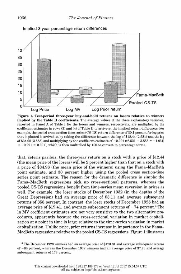
Log Price Log MV Log Prior return Figure 1. Test-period three-year buy-and-hold returns on losers relative to winners

implied by the Table II coefficients. The average values of the three explanatory variables, reported in Panel A of Table I for the losers and winners, respectively, are multiplied by the coefficient estimates in rows (3) and (4) of Table II to arrive at the implied return differences. For

example, the pooled cross section-time series (CS-TS) return difference of 30.1 percent for log price

that is plotted is arrived at by taking the difference between the log of $12.44 (2.521) and the log of $34.98 (3.555) and multiplying by the coefficient estimate of -0.291 ((2.521 - 3.555 = -1.034) x -0.291 = 0.301), which is then multiplied by 100 to convert to percentage terms.

that, ceteris paribus, the three-year return on a stock with a price of $12.44 (the mean price of the losers) will be 2 percent higher than that on a stock with a price of $34.98 (the mean price of the winners) using the Fama-MacBeth point estimate, and 30 percent higher using the pooled cross section-time series point estimate. The reason for the dramatic difference is simple: the Fama-MacBeth regressions pick up cross-sectional patterns, whereas the pooled CS-TS regressions benefit from time-series mean reversion in prices as well. For example, the loser stocks of December 1932 (in the depths of the Great Depression) had an average price of $3.11 and average subsequent returns of 358 percent. In contrast, the loser stocks of December 1928 had an average price of $19.41, and average subsequent returns of -74 percent.6 The ln MV coefficient estimates are not very sensitive to the two alternative procedures, apparently because the cross-sectional variation in market capitalization at a point in time is large relative to the time-series variation in market capitalization. Unlike price, prior returns increase in importance in the Fama- MacBeth regressions relative to the pooled CS-TS regressions. Figure 1 illustrates

6 The December 1928 winners had an average price of $123.81 and average subsequent returns of -80 percent, whereas the December 1932 winners had an average price of $7.73 and average subsequent returns of 173 percent.



the implied effects of the coefficient estimates using the two approaches.7 The third problem is that Conrad and Kaul's t-statistics are misstated in the

pooled CS-TS regressions. This is because each of the (up to) 35 observations in each cohort is assumed to be independent, when in fact there is substantial contemporaneous correlation in the residuals among the firms in a given cohort.

C. Price as a Proxy for Historical Returns

After replicating De Bondt and Thaler's finding that essentially all return reversals occur in January, Conrad and Kaul state on page 59 that "conditional on beginning of period prices, there is no relation between long-term returns and past performance. Therefore the January returns to losers and/or winners are not due to market overreaction." Unfortunately for this argument, essentially all low-priced stocks on the AMEX and NYSE are extreme losers relative to some price in their past, even if this is not true for some arbitrary interval, such as three years. To demonstrate this, in Table III we categorize firms on the basis of price, just as Conrad and Kaul do in their Tables V and VI. The low-priced portfolio has an average price of $2.40 and an average three-year prior return of a positive 10 percent. Measured from its high price during the previous ten years, however, these low-priced stocks are selling at an average of 75 percent below their peak. The median low-priced stock is selling at a discount of 84 percent relative to its peak. In other words, low-priced stocks are overwhelmingly extreme losers; so segmenting by price has no power to reject the overreaction hypothesis.

In an additional attempt to discern the impact of low-priced stocks on long-term returns, in unreported results, we have formed loser and winner portfolios on the basis of buy-and-hold returns after excluding all stocks with a price of $5.00 or less at the end of a ranking period. The subsequent buy-and-hold returns on the losers are 22 percent higher than on the winners, with all of the difference occuring in January. This number is much smaller than the 55 percent difference reported in Panel B of Table I. Thus, low-priced losers do have the highest returns, but they are not solely responsible for long-term return reversals.

III. Conclusion

As Conrad and Kaul contend, price can be used to predict future returns, and bid-ask spreads lead to an upward bias in monthly CARs on low-priced stocks (see Blume and Husic (1973), Blume and Stambaugh (1983), Keim and Stam- baugh (1986), Bhardwaj and Brooks (1992), and Dissanaike (1996) for related findings). Our disagreement with Conrad and Kaul concerns their argument

7 While we focus on the point estimates, the Fama-MacBeth t-statistic for the effect of prior returns in row (4) is only marginally significant. This reflects the fact that the procedure sacrifices power in order to achieve unbiasedness.



Table III

Average Price, Size, Prior Return, Test-Period Return, and Mean

and Median Price Relative to 10-year Highs, for Portfolios Formed

on the Basis of Price Fifty-eight cohorts of overlapping AMEX-NYSE data are used for portfolios formed on December

31, 1928 and each of the following 57 years, with the last portfolio formed on December 31, 1985.

Low-priced stocks are the 35 stocks with the lowest prices at the end of a particular formation

period. High-priced stocks are the 35 stocks with the highest prices. (In the event of ties, firms are

chosen in alphabetical order.) Price and market capitalization are as of the last trading day of the

formation period. For firms that are delisted before the end of the 3-year testing period, holding

period returns (HPRs) are calculated until the delisting. All returns are raw returns, unadjusted

for market movements. The price relative to the 10-year high is calculated as (Pformation date -

Phigh)YPhigh, where phigh is the highest month-end price during the previous 10 years listed on the CRSP monthly AMEX-NYSE tape. For example, a stock trading at $2.25 on the portfolio formation date with a high price of $35.00 during the prior 10 years would have a value of -93.6 percent. The median price relative to the 10-year high is the median of the 2,030 sample observations in the

respective portfolios.

Low-priced High-priced Difference Portfolio (1) Portfolio (2) (1) - (2)

Price $2.40 $127.98 -$125.58 Market Capitalization (in millions) $9.27 $2,066.55 -$2,057.28

Prior 3-Year HPRs 10.4% 104.9% -94.5% Test-Period 3-Year HPRs 102.2% 34.5% 67.7%

Mean Price Relative to 10-year High -75.3% -25.2% -50.1% Median Price Relative to 10-year High -83.5% -19.8% -63.7%

Proportion of AMEX firms during 1966-1986 91.3% 9.8% 81.5%

regarding the causality and magnitude of the effects, and their statistical significance in the context of long-term reversals.

Conrad and Kaul's methodology overstates the importance of ln Price in explaining subsequent cross-sectional returns. Their use of a pooled cross section-time series regression, in which price forecasts market returns, accounts for most of the different findings. Their procedures confound cross- sectional patterns with time-series patterns: the high returns on almost all stocks in the test-period beginning in 1932, when most stocks had low prices, and the low returns on almost all stocks in the test-periods beginning in 1929 and 1968, when most stocks had high prices. Furthermore, they misstate their t-statistics by ignoring the contemporaneous correlations of residuals of stocks from the same cohort year, and they introduce a survivor bias.

We provide direct evidence that the use of CARs compared to buy-and-hold returns for measuring prior and test-period returns is not driving De Bondt and Thaler's (1985) findings. Whereas monthly CARs on low-priced stocks are affected by bid-ask spread bias, they do not benefit from the advantages of compounding, and in this application, these two effects largely offset each other. Furthermore, when portfolios are formed on the basis of CARs, as De Bondt and Thaler and Conrad and Kaul do, the bid-ask spread bias results in



some low-priced stocks being classified as winners in spite of low ranking- period buy-and-hold returns, thereby lowering the power of tests. When buy- and-hold returns are used for forming portfolios and measuring subsequent return differences, losers outperform winners by more than when CARs are used. When price is used for forming portfolios, subsequent return differences are even larger.

In long-term return reversal studies, the losers with prices below $5 do have the highest subsequent buy-and-hold returns, with all of the extra return coming in January. After bull markets, few of the losers are in this low-price category, whereas after bear markets, many are. Thus, it is difficult to disen- tangle aggregate market mean reversion from price effects. Furthermore, restricting the analysis to January does not ameliorate this. As shown by Jegadeesh (1991), the phenomenon of aggregate stock market mean reversion occurs entirely in January.

More generally, when portfolios are formed on a single variable, the combined effects of correlated variables that are related to returns are present, overstating the impact of the single variable. This is true whether the variable is price (Blume and Husic, 1973), beta (Fama and MacBeth, 1973), size (Banz, 1981), prior returns (De Bondt and Thaler, 1985), earnings yield (Basu, 1977), book-to-market (De Bondt and Thaler, 1987), or whether a company recently went public (Ritter, 1991). The common theme in all of these papers is that "value" stocks have higher subsequent returns than "glamour" stocks. We do not address how much of the higher average returns to losers are a manifes- tation of equilibrium compensation for risk-bearing, and how much is due to overreaction. As Jones (1993) argues, this is a difficult question to answer.

REFERENCES

Ball, Ray and S. P. Kothari, 1989, Nonstationary expected returns: Implications for tests of market efficiency and serial correlations in returns, Journal of Financial Economics 25, 51-74.

Ball, Ray, S. P. Kothari, and Jay Shanken, 1995, Problems in measuring portfolio performance: An application to contrarian investment strategies, Journal of Financial Economics 38, 79-107.

Banz, Rolf W., 1981, The relationship between return and market value of common stocks, Journal of Financial Economics 9, 3-18.

Basu, Sanjoy, 1977, The investment performance of common stocks in relation to their price- earnings ratios: A test of the efficient market hypothesis, Journal of Finance 32, 663-682.

Bhardwaj, Ravinder K. and Leroy D. Brooks, 1992, The January anomaly: Effects of low share price, transaction costs, and bid-ask bias, Journal of Finance 47, 553-575.

Blume, Marshall E. and Frank Husic, 1973, Price, beta, and exchange listing, Journal of Finance 28, 283-299.

Blume, Marshall E. and Robert F. Stambaugh, 1983, Biases in computed returns: An application to the size effect, Journal of Financial Economics 12, 387-404.

Chopra, Navin, Josef Lakonishok, and Jay R. Ritter, 1992, Measuring abnormal returns: Do stocks overreact?, Journal of Financial Economics 31, 235-268.

Conrad, Jennifer and Gautam Kaul, 1993, Long-term market overreaction or biases in computed returns?, Journal of Finance 48, 39-63.

De Bondt, Werner and Richard Thaler, 1985, Does the stock market overreact?, Journal of Finance 40, 793-805.

De Bondt, Werner and Richard Thaler, 1987, Further evidence of investor overreaction and stock market seasonality, Journal of Finance 42, 557-581.



Dissanaike, Gishan, 1996, Are stock price reversals reallyasymmetric? A note, Journal of Banking and Finance 20, 189-201.

Fama, Eugene F. and James MacBeth, 1973, Risk, return and equilibrium: Empirical tests, Journal of Political Economy 81, 607-636.

Jegadeesh, Narasimhan, 1991, Seasonality in stock price mean reversion: Evidence from the U.S. and the U.K., Journal of Finance 46, 1427-1444.

Jones, Steven L., 1993, Another look at time-varying risk and return in a long-horizon contrarian strategy, Journal of Financial Economics 33, 119-144.

Keim, Donald B. and Robert F. Stambaugh, 1986, Predicting returns in the stock and bond markets, Journal of Financial Economics 17, 357-390.

Newey, Whitney K. and Kenneth D. West, 1987, A simple, positive semi-definite heteroskedasticity and autocorrelation consistent covariance matrix, Econometrica 55, 703-708.

Ritter, Jay R., 1991, The long-run performance of initial public offerings, Journal of Finance 46, 3-27.

White, Hal, 1980, A heteroskedasticity-consistent covariance matrix estimator and a direct test for heteroskedasticity, Econometrica 48, 817-838.


long-term market overreaction: the effect of low-priced stocks · the journal of finance . vol. li,...

Documents