long-term mapping techniques for ship hull inspection...
TRANSCRIPT

Long-Term Mapping Techniques for Ship Hull Inspection
and Surveillance Using an Autonomous Underwater
Vehicle
Paul OzogDepartment of Electrical Engineering and Computer Science
University of [email protected]
Nicholas Carlevaris-BiancoDepartment of Electrical Engineering and Computer Science
University of [email protected]
Ayoung KimDepartment of Civil and Environmental EngineeringKorea Advanced Institute of Science and Technology
Ryan M. EusticeDepartment of Naval Architecture and Marine Engineering
University of [email protected]
Abstract
This paper reports on a system for an autonomous underwater vehicle to perform in-situ,multiple session, hull inspection using long-term simultaneous localization and mapping(SLAM). Our method assumes very little a-priori knowledge, and does not require the aidof acoustic beacons for navigation, which is a typical mode of navigation in this type of ap-plication. Our system combines recent techniques in underwater saliency-informed visualSLAM and a method for representing the ship hull surface as a collection of many locallyplanar surface features. This methodology produces accurate maps that can be constructedin real-time on consumer-grade computing hardware. A single-session SLAM result is ini-tially used as a prior map for later sessions, where the robot automatically merges the mul-tiple surveys into a common hull-relative reference frame. To perform the re-localizationstep, we use a particle filter that leverages the locally planar representation of the ship hullsurface, and a fast visual descriptor matching algorithm. Finally, we apply the recently-developed graph sparsification tool, generic linear constraints (GLC), as a way to managethe computational complexity of the SLAM system as the robot accumulates informationacross multiple sessions. We show results for 20 SLAM sessions for two large vessels overthe course of days, months, and even up to three years, with a total path length of approx-imately 10.2 km.

1 Introduction
Periodic maintenance, structural defect assessment, and harbor surveillance of large ships is of great im-portance in the maritime industry because structural wear and defects are a significant source of lost rev-enue (Boon et al., 2009). Until recently, these tasks were carried out by periodic dry-docking, where a vesselis removed from the water for easy access to the entire ship hull. This task has recently evolved to includethe deployment of a variety of unmanned underwater robots to map and inspect the hull in-situ. Dueto the periodic nature of the inspection, surveys are often conducted every few months. Having a singleautonomous underwater vehicle (AUV) map an entire vessel within a short time frame may be impossi-ble. However, using multi-session mapping techniques would parallelize the inspection process, or allowpartial maps to be built as time allows. In addition, the sheer size of the final map would prevent a state-of-the-art simultaneous localization and mapping (SLAM) system from performing in real-time. Therefore,a computationally efficient and compact representation of the map is critical to maintain real-time map-merging performance in the long term.
The goal of this work is to extend our Hovering Autonomous Underwater Vehicle (HAUV) graph-basedvisual SLAM system to support automated registration from multiple maps via a method called multi-session SLAM. To maintain real-time performance, redundant or unnecessary nodes are marginalized fromthe factor-graph once the sessions are aligned into a common hull-relative reference frame. An overview ofour multi-session SLAM framework is illustrated in Fig. 1, including a visualization of how the estimatedtrajectory would align with a computer aided design (CAD) hull model. This framework is consistent,computationally efficient, and leverages recent techniques in SLAM research to create an extensive map.Our method has several advantages over long-baseline (LBL) and global positioning system (GPS) navi-gation methods. In essence, long-term hull-inspection with an AUV demands a hull-relative method fornavigation because a vessel’s berth may change with time.
We have laid the foundation of this paper in our earlier publications (Ozog and Eustice, 2013b, 2014). Here,we offer several improvements to our previous methodology, including:
• The use of a constraint between a plane and individual Doppler velocity log (DVL) beams.
• Periscope re-localization with the aid of pose-constrained correspondence search (PCCS).
• Exemplar views to maintain visual diversity in the merged graph.
• A quantitative evaluation of the effect of repeated application of generic linear constraints (GLC)for our application.
• Significantly more field data used in our evaluation. The surveys now span three years, with a totalpath length exceeding 10 km.
We start with a brief overview of relevant literature in Section 2. In Section 3, we summarize our singlesession SLAM framework and introduce our planar factor constraint, which substantially improves oursurvey results. We describe our overall approach for long-term hull-relative SLAM using the HAUV in Sec-tion 4. Here, we present how our SLAM system for the HAUV can be adapted for the GLC framework, thusenabling long-term mapping capabilities. Finally, in Section 5, we experimentally evaluate our approachusing real-world data, and conclude with a discussion in Section 6.
2 Related Work
We cover three broad areas of related work: (i) underwater surveillance using robots and underwater sen-sors, (ii) managing graph complexity for long-term SLAM, and (iii) merging intermediate SLAM graphsinto a larger map without a fixed absolute reference frame, for example, as provided by a GPS.

A
B
C
(a) SS Curtiss multisession SLAM result with three sessions (A,B,C)
A
B
C
(b) Merged graphs overlaid on CAD model
Figure 1: Multi-session SLAM overview. In (a), we show three different sessions aligned to a common frameusing our multi-session SLAM framework, with each color denoting a different session. A surface mission(‘A’), in blue, uses the periscope camera to capture images of the ship’s above-water superstructure. Twounderwater missions (‘B’ and ‘C’), in red and green, capture underwater images of the ship hull. The graypatches denote the planar features used in our novel planar constraints framework, described in §3.4. Tworepresentative images from the periscope and underwater camera are shown. In (b), we manually aligneda low fidelity CAD model of the ship for the sake of visual clarity, with the corresponding sessions coloredappropriately. Note that this CAD model is not used in our SLAM system.
2.1 Robotic Underwater Surveillance
Early work by Harris and Slate (1999) aimed to assess superficial defects caused by corrosion in large shiphulls using the Lamp Ray remotely operated vehicle (ROV). A non-contact underwater ultrasonic thick-ness gauge measured the plate thickness of the outer hull, and an acoustic beacon positioning system wasused for navigation. Since the early 2000’s, some focus has shifted from structural defect detection to theidentification of foreign objects like limpet mines. Sonar imaging sensors, in particular, have been success-fully deployed to detect foreign objects underwater (Belcher et al., 2001). In work by Trimble and Belcher(2002), a similar imaging technique was successfully deployed using the free-floating CetusII AUV. Like theLamp Ray, this system used a specifically-designed LBL acoustic beacon system for navigation around shiphulls and similar underwater structure. Additionally, Carvalho et al. (2003) used a probability-of-detectionmetric to assess the effectiveness of these sorts of acoustic-based sensors. Regardless of the specific robotused, the significant amount of infrastructure required for beacon-based navigation (Milne, 1983) hindersthe widespread use of these robotic systems in large shipping ports.

More recently, techniques in computer vision and image processing have been applied to various applica-tions in underwater inspection. Negahdaripour and Firoozfam (2006) used a stereo vision system to aid inthe navigation of a ROV, and provide coarse disparity maps of underwater structure. Ridao et al. (2010)used both a camera and sonar to inspect dams using an ROV, and employed bundle-adjustment techniquesand image blending algorithms to create mosaics of wall-like structures of a hydroelectric dam. Some ef-forts have even attempted to identify physical defects only from a single image. Bonnın-Pascual and Ortiz(2010) applied various image processing techniques to automatically identify the portions of a single imagethat appear to contain corrosion.
In addition to free-floating vehicles, there are some approaches that use robots that are physically attachedto the ship hull itself. Menegaldo et al. (2008, 2009) use magnetic tracks to attach the robot to the hull, buttheir hardware is limited to above-water portions of the hull. By contrast, Ishizu et al. (2012) developeda robot that uses underwater, magnetically adhesive spider-like arms to traverse the hull. Like previouslymentioned free-floating vehicles, this robot employs a stereo camera to assess the amount of corrosion. Hullinspection with high frequency profiling sonar is presented by VanMiddlesworth et al. (2013) where theybuild a 3D map and the entire pose-graph is optimized using submaps.
Although the main focus of this paper is on in-water hull inspection, there are other applications for long-term AUV-based surveillance and mapping in large area underwater environments. Autonomous vehiclespresent significant potential for efficient, accurate and quantitative mapping in arctic exploration (Kunzet al., 2009), Mariana Trench exploration (Bowen et al., 2009), pipeline inspection (Gustafson et al., 2011) andcoral reef habitat characterization (Singh et al., 2004). These studies were presented within the context ofa single-session SLAM application, however, the repeated monitoring and multi-session SLAM frameworkwe present here could be beneficial in those application domains as well.
2.2 Long-term SLAM for Extensive Mapping
Graph-based SLAM solvers (Dellaert and Kaess, 2006; Grisetti et al., 2007; Kaess et al., 2008; Kummerleet al., 2011) are popular tools in SLAM, however they are limited by computational complexity in manylong-term applications. As a robot explores an area and localizes within its map, pose nodes are continu-ally added to the graph. Therefore, optimizing a graph of modest spatial extent becomes intractable if theduration of the robot’s exploration becomes sufficiently large. A number of proposed methods attempt toaddress this problem by removing nodes from the graph, thus reducing the graph’s size. Recent empha-sis has been placed on measurement composition using full-rank factors, such as laser scan matching orodometry (Konolige and Bowman, 2009; Eade et al., 2010; Kretzschmar and Stachniss, 2012). Measurementcomposition synthesizes virtual constraints by compounding full-rank 6-degree of freedom (DOF) trans-formations, as shown in Fig. 2(a), however this operation is ill-defined for low-rank measurements, such asthose produced by a monocular camera, shown in Fig. 2(b). This is one of the primary motivations for thedevelopment of the factor-graph marginalization framework described by Carlevaris-Bianco and Eustice(2013a), called generic linear constraints (GLC), which address the low-rank problem.
The GLC method avoids measurement composition and works equally well using full-rank and low-rankloop-closing measurements. This is a critical requirement for the HAUV application because low-rankfactors from either a monocular camera or an imaging sonar are the primary means of correcting naviga-tional error from the DVL. Furthermore, measurement composition tends to re-use measurements whensynthesizing virtual constraints. Doing so double-counts information and does not produce the correctmarginalization in the reduced SLAM graph.
Previous studies of large-scale SLAM suggest solving SLAM using multiple maps to efficiently and consis-tently optimize very large graphs. The first method for constructing a large-scale map involves the use ofsubmapping techniques, i.e., building local maps and then stitching the local maps together to build largermaps. This type of submap technique was originally proposed by Leonard and Feder (1999) to reduce thecomputational cost by decoupling the larger maps into submaps. This work was further developed into

(a) (b)
Figure 2: This figure shows that the measurement composition technique, often used in variable marginal-ization in graph-based SLAM, is undefined for low-rank monocular camera measurements, as used in thiswork. For generating the green end-to-end 6-DOF transformation in (a), one simply has to compound theintermediate 6-DOF relative-pose transformations, in blue. This cannot be done for the intermediate 5-DOFmeasurements shown as red arrows in (b). In this case, computing the end-to-end baseline direction ofmotion is ill-posed because it depends on the scale at each camera measurement, which is not known.
the Atlas framework by Bosse et al. (2004) where each submap is represented as a coordinate system in aglobal graph. For example, Bosse and Zlot (2008) developed a two-level loop-closing algorithm based onthe Atlas framework, while Neira and Tardos (2001) introduced a way to measure joint compatibility, whichresulted in optimal data association. Examples of underwater submap applications include vision (Pizarroet al., 2009) and bathymetry maps from acoustic sensors (Roman and Singh, 2005). Kim et al. (2010) used asimilar submapping approach, except in the context of a factor-graph representation of cooperative SLAM.They used so-called anchor nodes, which are variable nodes representing the transformation from a commonreference frame to the reference frame of each vehicle’s SLAM graph. Anchor nodes are nearly identicalto base nodes introduced by Ni et al. (2007). They are a very simple way to extend observation models toperform submap alignment, which is why our multi-session SLAM approach (discussed in §4) formulatesthe session alignment using anchor nodes.
To efficiently perform multi-session SLAM in the absence of a readily-available absolute position referencerequires an initial data-association step. By doing so, each map can be expressed into a common frameof reference, thus bounding the search space for identifying additional data associations. Recently, visualinformation has been exploited in data association by providing an independent loop-closing ability basedupon appearance. Nister and Stewenius (2006) introduced a framework that used a bag-of-words (BoW)representation of images to quickly compare the histogram of words between two images using vocabularytrees. Cummins and Newman (2008) used a generative model to describe the co-occurrence of words inthe training data. They developed the popular Fast Appearance-Based Mapping (FAB-MAP) algorithm,which frames the problem as a recursive Bayes filter and showed that their system can leverage temporalinformation with or without a topological motion prior. Both of these methods have become a commonpractice for loop-closure detection in real-time SLAM front-ends.
Our approach also shares some similarity with methods that maintain visual diversity in long-term SLAMgraphs. GraphSLAM by Thrun and Montemerlo (2006) presents some early work on a large urban areawith visual features. The method, however, was an offline approach with conventional optimization meth-ods. Our work has more connection to recent online approaches such as the one introduced by Konoligeand Bowman (2009). They represent a place in the SLAM graph as a collection of exemplar views. Thisencourages visually diverse keyframes in the SLAM graph, thus increasing potential matchability as moreimages are collected by the robot. Furthermore, this approach limits the number of views to be less than auser-defined parameter, which keeps the graph size bounded.

(a) (b)
Figure 3: The Bluefin Robotics HAUV (shown in (a)) is specifically designed for in-situ underwater hull andharbor inspection and requires no pre-existing infrastructure (e.g., acoustic beacons), to localize. Instead, ituses a DVL for hull-relative navigation, which differentiates it from other similar inspection robots. In (b),we show the relative size of the vehicle compared to a typically-sized vessel.
3 Underwater Visual SLAM with Planar Constraints
In our trials, we use the HAUV (Fig. 3) developed by Bluefin Robotics. The HAUV is a free-floating vehiclethat requires no existing LBL infrastructure for localization (Hover et al., 2007). Instead, the HAUV uses aDVL as its primary navigation sensor, which can operate in a hull-relative or seafloor-relative mode. Thisallows the robot to inspect a variety of underwater infrastructure: ship hulls, pilings, or harbor surveillance.The vehicle is equipped with two monocular cameras so that it can switch between below-water and above-water images. The periscope camera is fixed with a static angle allowing the robot to capture superstructureand above-water features. The underwater camera is mounted on a tray along with the imaging sonar andDVL. During a mission, the tray is servoed such that both the DVL and camera always point nadir to thehull while the robot keeps a fixed distance.
In this section, we introduce the overall system, including the SLAM back-end, and camera and plane con-straints. The illustration of the pose-graph framework is given in Fig. 4. The robot is provided with camera,planar, and odometry measurements together with absolute measurements on depth and attitude. Follow-ing a brief illustration of each module, we specifically focus on the planar constraints that substantiallyimprove mapping and localization performance.
3.1 State Representation
For the remainder of this section, let xij = [xij , yij , zij , φij , θij , ψij ]⊤ be the 6-DOF relative-pose of frame j
as expressed in frame i, where x, y, z are the Cartesian translation components, and φij , θij , and ψij denotethe roll (x-axis), pitch (y-axis), and yaw (z-axis) Euler angles, respectively. Ri
j is the rotation matrix that
rotates a vector in j’s frame to a vector in i’s frame, and tiij is the translation from i to j as expressed in i’s
frame. Finally, g will refer to the global, or common, reference frame.

full-state prior
absolute meas. (depth, pitch, roll)camera meas.
planar range meas.pose-to-plane meas.
piecewise-planar meas.odometry meas.
Figure 4: An illustration of a multi-session factor-graph with camera, planar and other measurements.Orange, blue, and green variable nodes correspond to planes, vehicle poses, and anchor nodes, respectively.The top half nodes correspond to a prior session (reference frame a), while the bottom half belong to asubsequent session (reference frame b). Factor nodes are shown as black circles, along with the type ofobservation encoded as a script character. The use of odometry and prior factors is common-practice inpose-graph SLAM so these are not covered in detail in this paper. The camera and planar measurementsare discussed in more detail in §3.3 and §3.4, respectively.
3.2 SLAM Back-end
The HAUV is equipped with a variety of sensors: a DVL and inertial measurement unit (IMU) for odometry,a pressure depth sensor, two cameras for 3D bearing measurements, and an imaging sonar. The use of thesesensors for SLAM is described in detail by Johannsson et al. (2010) and Kim and Eustice (2009). SLAM aimsto correct for any accumulated navigational error when the robot senses environmental features it has seenpreviously. The DVL measures four beam ranges, along with four body-frame velocities. These rangemeasurements can also be converted to a sparse 3D point set, which allows us to fit local planar patches tothe DVL data.
The SLAM system used on the HAUV has evolved from an offline filtering-based approach with manualdata association (Walter et al., 2008), to a real-time factor-graph optimization framework that supports bothsonar and monocular camera measurements automatically (Hover et al., 2012). Currently, our SLAM sys-tem uses the incremental smoothing and mapping (iSAM) algorithm as the optimization back-end (Kaesset al., 2008; Kaess and Dellaert, 2009; Kaess et al., 2010).
3.3 Camera Constraints
The previously-mentioned underwater and periscope cameras can both be used to derive spatial constraintsfrom two-view feature correspondence. The underwater environment is particularly challenging becauseit does not always contain visually useful features for camera-derived measurements. To alleviate thisissue, Kim and Eustice (2013) allowed for greatly increased computational performance by only consideringvisually salient keyframes in the visual SLAM pipeline. They derived a local saliency score using a coarseBoW representation of each keyframe from speeded-up robust features (SURF) descriptors (Bay et al., 2006).To derive two-view camera constraints from overlapping images, the system searches for correspondencebetween keyframes using the scale-invariant feature transform (SIFT) descriptor (Lowe, 2004). A scenedepth prior based upon the DVL and a relative-pose prior based on the SLAM estimate offer a constrainedputative correspondence search that is faster and more consistent than typical appearance-only randomsample consensus (RANSAC)-based approaches (Eustice et al., 2008; Carlevaris-Bianco and Eustice, 2011).

From two overlapping images taken from our monocular camera, we can derive a spatial constraint, mod-ulo scale, between the vehicle poses from which those images where taken. This measurement thereforehas five DOFs: three rotations, and a vector representing the direction of translation that is parameterizedby azimuth and elevation angles.
We have found that adding camera measurements with low baseline can potentially produce outlier mea-surements. These outliers are occasionally not identified with a Mahalanobis distance check prior to theiraddition to the SLAM graph. We therefore use the robust back-end method known as Dynamic CovarianceScaling (DCS) (Agarwal et al., 2013). This method is based on the work by Sunderhauf and Protzel (2012),which employs switching variables to turn on and off measurements by scaling the information matrix forloop-closing measurements. DCS does this in closed form, which avoids having to increase the dimension-ality of the state to estimate the scale variables. Thus, the robust monocular camera factor between posesxgi and xgj is:
χ2DCSij
=∥∥∥z5dofij − h5dof (xgi,xgj)
∥∥∥2
1
s2ij
Ξzij
, (1)
where h5dof (xgi,xgj) = [αij , βij , φij , θij , ψij ] is the predicted baseline direction of motion azimuth αij , ele-vation βij , and the relative Euler angles φij , θij , ψij , and 1
s2ij
Ξzijis the DCS scaled measurement covariance
matrix. Agarwal et al. (2013) show that the covariance scale variable, sij , is given by
sij = min
(1,
2Φ
Φ + χ2l
),
where χ2l is the unscaled chi-squared error, computed from (1) using the unscaled measurement covariance,
Ξzij. Higher values of the parameter Φ make it more likely to accept loop closures. For our field trials, we
choose Φ = 5; however, values between 1 and 10 produce nearly identical results.
3.4 SLAM with Planar Segments
To further constrain the vehicle’s trajectory, we use planar patches as nodes in the SLAM graph using apiecewise-planar model (Ozog and Eustice, 2013b), which is summarized in Fig. 5. This method providesan explicit representation of the ship hull surface in the factor graph, and produces accurate and efficientmaps using only a sparse 3D point cloud (such as one produced by the underwater DVL navigation sensor).Furthermore, this method preserves the overall curvature of the ship’s exterior hull, assuming that the robothas coarse prior knowledge on the side-to-side and top-to-bottom characteristic curvature of the surface.This distinguishes our work from other planar SLAM approaches (Weingarten and Siegwart, 2006; Trevoret al., 2012) in two ways. First, other methods make use of a much more data-rich 3D laser scanners ordepth cameras. Second, these other approaches are experimentally evaluated in structured environments,like office buildings, that contain many planar walls at sharp angles to each other. Unfortunately, theseapproaches require that the planes be directly observed from two or more views. However, this is oftennot achievable in ship hull inspection because (i) the hull is smoothly curved, and (ii) the DVL’s field ofview is both more narrow and more sparse than a typical laser scanner or depth camera. In this section, weexplain the plane constraints from a single session point of view, but another significant strength of theseconstraints are in robust registration that allows for multi-session SLAM, which will be discussed in §4.
3.4.1 Plane Composition Operators
The planar observation models used in this paper involve expressing planes in multiple frames of reference.In this section, we describe these operations in detail. Let πik be the plane indexed by k, expressed withrespect to frame i. When i is the global frame, g, this plane corresponds to a variable node in our factor-graph. We parametrize the plane πgk = [nx
gk, nygk, n
zgk]
⊤ using three numbers, where nxgk, nygk, and nz
gk

(a)
(b)
Figure 5: The method in this paper represents the ship hull surface as a collection of locally planar fea-ture patches (gray), with a simple assumed prior on the characteristic curvature model. The residual errorof two co-registered planes are weighted in such a way so that only errors that extend outside of the de-viation explained by the characteristic curvature are significant. The method relies on two characteristicradii parameters: one for the azimuth (side-to-side variation, shown in (a)), and one for elevation (top-down variation, shown in (b)). Ozog and Eustice (2013b) show that the performance of this approach is notoverly sensitive to these user-defined parameters.
are the x, y, and z components of the (non-unit) normal vector to the plane k, expressed in the global-frame, g. We do not use the popular Hessian normal form simply because it is parameterized by fournumbers, despite having only three degrees of freedom. This over-parameterization would therefore resultin a singular covariance matrix. The Hessian normal form is given by: n
⊤x = −p for any point x that
lies on the plane, where n is the unit normal of the plane, and p is the distance of the plane to the origin.Conversely, our parameterization uses only three numbers. We simply scale the unit-normal by the distanceto the origin, yielding what we denote as the π symbol. With our parameterization, we have π
⊤x = −‖π‖2
for any point x on the plane.
The frame of reference of the plane is denoted with a subscript whereby the plane indexed by k as expressedwith respect to some frame i is denoted πik. If one wishes to express a plane in a different frame of reference,one simply applies the ⊟ and ⊞ operators, which take as input a 6-DOF pose and 3-DOF plane. Let xij ⊟
πik = πjk, where
πjk = xij ⊟ πik =
(ti⊤ij πik + ‖πik‖
2)Rj
iπik
‖πik‖2.

The ⊟ operator is commonly used to evaluate factor potentials, discussed in the next section. We also definethe ⊞ operator, where xij ⊞ πjk = πik. This can be expressed in terms of the ⊟ operator by
xij ⊞ πjk = ⊖xij ⊟ πjk,
where ⊖ is the pose-inversion operation (Smith et al., 1986). The ⊞ operator is commonly used to transformplane measurements from the vehicle frame to the global, but not to evaluate factor potentials.
3.4.2 Planar Constraints between Poses and other Planes
In this section we describe observation models used to add measurements to our SLAM graph. A binaryfactor potential of the form
Ψ(xgi,πgl; zπil,Σzπil
) = ‖zπil− (xgi ⊟ πgl) ‖
2Σzπil
(2)
is used when the DVL sensor determines a good planar fit of a sliding time-window of 3D points. Thecovariance matrix, Σzπil
, is determined by first-order approximation of a function that fits a plane from the3D points, which are assumed to be corrupted by Gaussian noise.
A piecewise-planar factor potential is similarly used to constrain the surface normals of two plane nodeswith respect to a common pose node. It is given by the expression
Ω(xgi,πgk,πgl;Wijkl) =
‖ (xgi ⊟ πgk)− (xgi ⊟ πgl) ‖Wijkl. (3)
A weight matrix, Wijkl, is based on the characteristic curvature of the ship hull. It is a function of twovehicle poses from which the planes k and l were observed (that is, i and j, respectively):
Wijkl = diag(∆2
x,∆2y,∆
2z
)+CΣijC
⊤,
where Σij is the joint covariance between poses i and j. C is the Jacobian of the function c ( · ) that is asimple curvature model of the surface being observed. Since the two measured planes will not be perfectlycoplanar due to surface curvature, it is a simple way to take this into account when computing error fromthe ⊟ operator described in §3.4. This approach is illustrated in Fig. 5, and the mathematical formulation ofthe curvature model is
∆x
∆y
∆z
= c (xgi,xgj ;πik,πjl, ra, re) = πjl −
xij ⊟ trans
dir (πik) +
tiijy/ratiijz/re
0
,
where dir( · ) converts a 3-dimensional Cartesian vector to one expressed in 3-dimensional spherical coor-dinates: azimuth, elevation, and distance to the origin. Conversely, trans( · ) converts spherical coordinatesto Cartesian. See §A.1 for the full definition of these functions. The user-defined characteristic radii forazimuth and elevation are denoted ra and re, respectively. For the experimental results in this paper, weuse ra = 322 m and re = 7 m. Similar to what is described in Ozog and Eustice (2013b), the results pre-sented in this paper are almost identical so long as ra and re are within the same order of magnitude asthese provided values.
3.4.3 Range Constraints between Planes and Poses
In the event that fitting a plane to a point cloud is ill-conditioned, as is the case when all points are colinear,or when there is only a single point, we use a simple ray-tracing method to constrain a plane with theseill-conditioned DVL beams. This is illustrated in Fig. 6.

Figure 6: Given plane k and DVL pose d in the global frame, the points of intersection for each ray canbe computed so long as the ray origin and direction are known using (4). We can compare the predictedrange to the DVL-measured range, and use this as a spatial constraint between the pose and plane. Thisis particularly useful when the points detected by the plane are ill-conditioned for fitting a plane (such asonly two DVL beams that will always lie on a line, as in this figure).
(a) With range constraints (b) Without range constraints
Figure 7: In practice, we find the HAUV may only successfully measure the top two DVL returns — espe-cially when surfaced. Here, we show the benefits of leveraging this information in the context of SLAM. Ineach figure, the viewpoint is from stern-to-bow, and green lines encode the invocation of a range constraint.In (a), two surface missions are well-aligned, whereas in (b), there is some noticeable drift, highlighted inred. In each figure, black dots denote pose nodes in a sparsified graph using the GLC method discussedin §4.1.
Let rin be the n-th unit-norm ray expressed in pose frame i. If rin is known to intersect with plane πik, then
we can compute the predicted ray length, lrin
, by tracing the ray until it intersects with the surface. Becausethe surface is planar, we can derive a closed-form expression for the length:
lrin
(xij ,πik; r
in
)=
‖xij ⊟ πik‖
ri⊤n (xij⊟πik). (4)
The resulting factor potential between pose j and plane k is computed by weighting the difference betweenthe observed beam range, zl
rin
, and the predicted range from above:
Φ
(xij ,πik; zl
rin
, σzlrin
, rin
)=
zl
rin
− lrin
(xij ,πik; r
in
)
σzlrin
2
, (5)
where σzlrin
is the standard deviation of the range measurement noise from the nth beam.

Intuitively, this factor potential is less informative than the piecewise planar factor defined in (3). However,in the event that a plane is not observable from the DVL’s point cloud, it still provides a useful constraintfor the SLAM trajectory if a local planar patch has been previously established. In practice, we use thisconstraint in the event that the incident angle for the bottom two DVL beams is too large, which we findcan happen when the HAUV is at the surface. An example of the benefit of this information is shownin Fig. 7.
4 Multi-session SLAM for Long-term Hull Inspection
The typical use case for the SLAM system discussed above is for single-session surveys. When the robotbegins a new survey minutes or days after the previous survey, the navigation is reset and all the infor-mation from the previous map is no longer used in navigation correction. For long-term or multi-robotapplications, this is detrimental for two reasons. First, there is less information for the robot to correct itsnavigation. Second, each session has a different local reference frame. If a particular area for one of thesesurveys demands attention, it requires a human-in-the-loop to identify where the area of interest lies ina hull-relative reference frame. It is therefore beneficial, though challenging, to have the surveying robotbuild each map with respect to the same reference frame. In this section, we present: (i) an accurate andefficient global localization system to make the initial alignment, (ii) surface-based SLAM techniques tomake the real-time alignment robust and accurate, and (iii) managing the computational complexity ofoptimizing long-term SLAM graphs.
To illustrate how these techniques are used in practice during real-world operations, the following is a high-level outline of our multi-session SLAM system: (i) load past sessions as a SLAM graph, (ii) sparsify thegraph with GLC, (iii) deploy the HAUV and start building a separate, unaligned pose-graph, (iv) localizeto the past session with an initial guess of the alignment, and (v) refine alignment using monocular camerameasurements and piecewise-planar constraints on anchor nodes. These steps are illustrated in Fig. 8.
GLC has been thoroughly-evaluated on standard SLAM graphs containing pose nodes and landmarknodes. However, the graphs used in this work are significantly more nonstandard because they containanchor nodes, planar nodes, and planar observation models. This section will also describe how GLC canbe used with these aspects of our SLAM system.
4.1 GLC-based Approximate Node Removal
A detailed derivation and computational performance analysis of GLC node marginalization and removalcan be found in Carlevaris-Bianco and Eustice (2013a,b). GLC-based graph sparsification starts with an n-ary factor that captures the information within the elimination clique following marginalization. In short,this n-ary factor is computed by considering all the measurements contained in the Markov blanket of thenode that is to be marginalized. To handle low-rank measurements, this method computes eigenvalue-decomposition of the induced target information, Λt, and forms a generic linear observation model for then-ary factor:
zglc = Gxc +w′, (6)
where w′ ∼ N (0, Iq×q), G = D1/2U⊤, Λt = UDU⊤, q is the rank of Λt, and xc is the current linearization
of nodes contained in the elimination clique. UDU⊤ is the Eigendecomposition of Λt, where U is a p × qmatrix of Eigenvectors and D is a q × q diagonal matrix of Eigenvalues. To preserve sparsity in the graph,the target information Λt is approximated using a Chow-Liu Tree (CLT) structure, where the CLT’s unaryand binary potentials are represented as GLC factors. These resulting unary and binary factors replace thenode’s original surrounding factors.

Load a graph Start a newmission
Make aninitial alignment Refine alignment
(a) Multi-session SLAM diagram
(b) Sparse graph loaded (factors not rendered)
(c) Unaligned pose-graph
(d) Initial alignment to sparse graph
(e) Refine alignment and complete survey
Figure 8: Depiction of multi-session SLAM using the techniques provided in §4. The red region in (d)denotes the point of map reacquisition, where the robot determines a rough initial alignment to the graphfrom (b). We refine this alignment in real-time using the same techniques as our single-session system fromprevious work. Once the session from (e) is complete, we sparsify and repeat the process with additionalsessions.
GLC optionally supports node reparameterization into a local reference frame around xc when evaluatingthe observation model from (6). This avoids committing to a world-frame linearization if the nodes arenot well-optimized. Instead, nodes are linearized about a local relative-frame transformation. This relativetransformation arbitrarily picks a single pose node in the elimination clique as the common frame. Forplanar nodes, we use the ⊟ operator to express planes with respect to a root node. In the next section, wedescribe how to support anchor nodes in GLC’s reparameterization step.

(a) Factor-graph with anchor nodes (b) Factor-graph with global reference frame, g
Figure 9: A factor-graph topology for a simple SLAM example involving two sessions, A (left side) andB (right side). In (a), the graph encodes the distribution from (7), where each session has an associatedanchor node. This graph can be converted to a global representation in (b) without any loss of informationusing (9). The only discarded factors are the full-state prior factors in session B and on the anchor nodexga. These prior factors have little probabilistic importance and function primarily to keep the SLAMinformation matrix non-singular.
4.2 Global Multi-session SLAM from Anchor Nodes
For a robot or multiple robots performing multi-session SLAM, a pose-graph containing anchor nodes is apopular method to align multiple relative graphs (Kim et al., 2010). In this approach, each robot session hasan associated anchor node. An anchor node is a node containing the transformation from a global referenceframe to the corresponding session’s reference frame. The important advantages of anchor nodes overglobal multi-session SLAM, where all sessions are expressed in a common frame, are (i) faster convergenceof the nonlinear least-squares solver, and (ii) individual sessions can optimize their pose graphs before anyconstraints between them are observed.
For a two-session case consisting of sessions A and B, the factor-graph containing anchor nodes,from Fig. 9(a), encodes a probability distribution of the form
p(X | ZA, ZB, ZAB, PA, PB, Pga) =
p(xga,xa1A ,xa2A , . . . ,xaNA,
xgb,xb1B ,xb2B , . . . ,xbMB| ZA, ZB, ZAB, PA, PB, Pga), (7)
where xga is an anchor node representing the 6-DOF transformation from the global-frame, g, to the refer-ence frame a of session A. xaiA is the 6-DOF relative-pose from frame a to frame i of session A. X denotesthe set of variable nodes in the factor graph (i.e., the unknowns). ZA and ZB denote the sensor and odom-etry measurements contained in sessions A and B, respectively, and ZAB denotes the sensor measurementsbetween nodes in sessions A and B. PA and PB denote full-state priors in sessions A and B, and Pga denotesthe full-state prior on the anchor node, xga. Finally, N and M are the number of nodes in sessions A and B,respectively, not including the anchor node (Fig. 9).

The parameterization from (7) is somewhat inconvenient because in order to place the nodes into a commonframe (when visualizing the distribution, for instance, or when computing the expected information gainof a measurement between two nodes), a sparse nonlinear function, f , must be applied to the distribution:
µf(X) =
xga ⊕ xa1A...
xga ⊕ xaNA
xgb ⊕ xb1B...
xgb ⊕ xaMB
, (8)
where ⊕ is defined in Smith et al. (1986) as the compounding operation. The covariance of the resultingdistribution is computed to first order as
Σf(X) = JfΣXJ⊤f ,
where Jf is the Jacobian of µf(X).
Extending this analysis to more than two sessions is trivial. It is also straightforward when X containsplane nodes. In this case, the sparse nonlinear function f contains the ⊞ operator discussed in §3.4.
For convenience, we alter the distribution so that all nodes are in a common frame. Along with simplify-ing path planning, visualization, and hypothesizing informative measurements, doing so allows for trivialapplication of the GLC reparameterization suggested by Carlevaris-Bianco and Eustice (2013b). This alter-ation is illustrated in Fig. 9. First, we reduce the state variables using (8), effectively removing the anchornodes from the factor-graph. Next, we remove the full-state priors for nodes in session B and the anchornode in session A, leaving us with the distribution
p(X ′ | ZA, ZB, ZAB, PA) =
p(xg1A ,xg2A . . . ,xgNA,
xg1B ,xg2B . . . ,xgMB| ZA, ZB, ZAB, PA), (9)
In this way, none of the sensor measurements are discarded when converting the relative pose-graphs tothe global-frame. In practice, we perform this operation immediately after the robot completes a survey,and before performing offline GLC-sparsification.
4.3 Reacquisition to Sparsified Graph by Particle Filtering
This section describes how we accomplish the initial alignment step illustrated in Fig. 8(d). Once a graphhas been sparsified using GLC, we use a particle filter to estimate a distribution of likely poses in the refer-ence frame of the past session. Our particle filter is based on a classic Monte-Carlo localization framework.We use odometry, depth, pitch, and roll measurements derived from sensors to propagate particles to theirnext state. Our particle filter approach is summarized in Fig. 10.
4.3.1 Weighting particles from planar measurements
To weight the particles as new plane measurements are observed, we use a method similar to the computa-tion of potentials used in our factor-graph, described in §3.4. When a plane-fitting measurement, zπik
from(2), is received by the particle filter, it finds the nearest neighboring pose node i according to
i = argmini∈IΠ
‖tggpi− t
ggi‖,

(a) Unoccupied free space around outer hull (b) Initial particle distribution
(c) Particle distribution at start of first trackline (d) Particle distribution at end of first trackline
Figure 10: Particle filter reacquisition into a previous session SLAM graph. We improve the efficiency ofour particle filter by computing a simple occupancy grid, shown in (a), based upon the planar features ofthe sparsified graph. Only the grid cells that lie less than 3 m from of surface of the nearest plane maycontain particles from the initial distribution. We uniformly distribute particles, shown as red dots in (b),over the cells from (a). When the new survey begins, the particles are weighted based on their compatibilitywith planar measurements. In (c) and (d), particles are overlaid on the pose-graph where the black dots aregraph nodes. Over time, the distribution of particles will tend toward a smaller set of candidate keyframesto search.
where IΠ is the set of pose indices in the GLC-sparsified graph that have a corresponding plane. Finding theminimum over all IΠ is quite slow for large graphs, so this operation is approximated using a k-dimensional(KD)-tree from the FLANN library (Muja and Lowe, 2009).
Next, we take i′ to be the index of the plane that is observed from pose i. Finally, we set the weight, wpi, by
computing the Mahalanobis distance between the observed and expected planar measurement:
wpi= ‖zπpik
− (xgi ⊟ xgi′) ‖2Σii′
.
To get the initial distribution of particles, we compute a simple binary 3D occupancy grid from the GLC-sparsified graph, and remove any particles that are assigned to occupied cells. For each cell, if it lies outsidethe nearest pose-plane pair, that cell is marked as “not occupied.” Otherwise, the cell is marked as “occu-pied.”
The particle filtering approach is summarized in Fig. 10. We find that the particle distribution tends towarda narrow band at the proper depth. With the addition of planar measurements, this distribution can cullout ends of the ship that do not agree with the structural information observed by the robot. This behavioris shown in Fig. 10(c) and Fig. 10(d).

Algorithm 1 Match current keyframe to candidate keyframes based on particle distribution
1: Input: Particles p1 . . . pN , current keyframe k, set of all pose indices in GLC-sparsified graph with correspondingkeyframe IK
2: S← ∅
3: for pi ∈ p1 . . . pN do4: S← S ∪ NEIGHESTNEIGHBOR(pi, IK ) ⊲ Uses kd-tree5: end for6: Output: FINDBESTMATCH(k, S) ⊲ Uses GPU
(a) Planar scene and relative-pose prior for upward-lookingperiscope
(b) 3-σ confidence regions for 2D point transfer from the past keyframe (left) tothe candidate keyframe (right).
Figure 11: When searching for putative correspondence, the geometry of the periscope images can be ex-ploited since the variation within relative-poses from the same place is mostly in the y-axis (“side-to-side”).First, we can back-project the points from the past camera pose assuming a planar scene, as shown in (a).Second, we model the relative-pose uncertainty as a Gaussian ellipsoid and project this uncertainty as 2Dellipses in the candidate keyframe’s image plane, shown in (b). We can search for putative SIFT correspon-dences within these ellipses, rather than searching the entire image.
4.3.2 Planar Scene Prior for Putative Correspondence in Periscope Images
The uncertainty between two matching poses in the initial alignment step can be modeled as a covarianceellipsoid with high variation in the side-to-side axis. The other dimensions are well-instrumented withdepth and IMU sensors. This can be probabalistically modeled by assuming a zero-mean transformationbetween the two candidate poses with an appropriately-constructed transformation covariance matrix.
If we further approximate the periscope scene as purely planar, we can back-project points from the firstcandidate camera pose onto a known plane in 3D space. We can then re-project these points into the im-age of the second candidate camera, and propagate the covariance terms using an Unscented Transform(UT) (Julier, 2002; Ozog and Eustice, 2013a). This process is illustrated in Fig. 11, and is a special case of thePCCS described by Eustice et al. (2008). Note that this technique is only useful for the periscope images,where the scene is large as compared to the underwater images. Effectively, this constrains correspondingfeatures in periscope images to share similar pixel row indices. By contrast, correspondences in underwa-ter images could have very different row indices. Therefore, for the underwater case, we revert to a purelyputative correspondence search because it runs faster on a graphics processing unit (GPU).
4.3.3 Keyframe Matching with SIFT and RANSAC
After resampling, if the distribution of particles is sufficiently small in the x, y plane, we find the set ofall images contained in the particle distribution. For our experiments, we build this set when the square-root of the determinant of the marginal x, y covariance is less than 250 m. This threshold tends to pro-duce a keyframe set that contains about 100 images and takes roughly three to four seconds to perform a

Algorithm 2 Sparsification algorithm
Input: Alignment of two SLAM sessions, A+B. A is the pre-sparsified prior session and B is the current session.Output: Set of all nodes to maginalize, S. Updates exemplar views.
1: N = SPATIALLYREDUNDANTNODES(B)2: for node in B and not in N do3: views← NEARESTEXEMPLARCLUSTERORNEW(A, node)4: if ANYVIEWCLOSEINTIME(views, node) or not VISUALLYSALIENT(node) then5: S← S ∪ node6: else7: S← S ∪ PUSH(views, node) ⊲ “views” is fixed-size FIFO. If views is full, PUSH returns popped node.8: end if9: end for
10: GLCREMOVE(A+B, S ∪ N)
brute-force search. This step, denoted as FINDBESTMATCH in Algorithm 1, uses a GPU for SIFT descriptorextraction and matching, and finally rejects outliers by using an eight-point RANSAC algorithm to fit a fun-damental matrix between the current keyframe and a candidate image extracted from the set. The keyframewith the most inliers above a threshold is selected to be the best match. For our experiments, we choosea threshold of 12 inliers to avoid false positives. If no matches are found, the search is repeated when therobot moves approximately one meter from the point at which the previous search was attempted. Doingso prevents redundant searching.
4.3.4 Maintaining Keyframe Diversity in Merged Graph
Maintaining diversity in the keyframes associated with vehicle pose nodes in the SLAM graph is criticallyimportant for the particle filter to successfully localize. To maintain diversity of the images associated withnodes in our merged SLAM graph, we use a simple algorithm that is inspired from the work by Konoligeand Bowman (2009). In their approach, a robot maintains a maximum number of recent exemplar viewsusing a simple image closeness measure and a least-recently used cache algorithm. By contrast, our al-gorithm only adds additional exemplar images if the keyframe is visually salient and sufficiently distantin time to all others from the same neighborhood (lines 3 and 4 in Algorithm 2). This approach producesgraphs whose sizes are closely bound to the size of the ship hull and maintains nodes with high utility formulti-session SLAM.
In practice, Algorithm 2 tends to preserves nodes that are both visually salient (for potential camera mea-surements), and useful for their locally planar structure (for piecewise planar or planar range measure-ments). Intuitively, this algorithm simply keeps the most recently-used views in a fixed-size neighborhood.An example of the how we maintain image diversity for the graphs used in the experimental results sectionis shown in Fig. 12.
This algorithm has various user-defined parameters. For the HAUV datasets, we chose a threshold of 1.5 mto decide if a node is spatially redundant (line 1 in Algorithm 2), and the maximum number of views perneighborhood as three (line 7 in Algorithm 2). We used the local saliency metric described by Kim andEustice (2013) as the method for determining if an image is visually salient.
5 Experimental Trials
This section describes experimental trials with the HAUV performing automated inspections on theUSS Saratoga and SS Curtiss vessels depicted in Fig. 13. We present an extensive multi-session SLAM graphmerged on these two vessels over three years. Further analysis on the proposed method is followed in termsof complexity, comparison to other vision-based loop-closure methods, and map accuracy in sparsification.

Figure 12: Illustration of exemplar views for the GLC SS Curtiss graphs. Two example view neighborhoodsare circled in blue. Exemplar views within these neighborhoods (shown above), are noticeably differentbetween 2011 and 2014. We manually outlined common regions in white for illustration. In the left example,different bio-foul patterns are growing on the same circular structure on the hull bottom. In the rightexample, SIFT features are detected on the pitting from the 2014 data, however, this pitting is not presentin the 2011 data.
(a) USS Saratoga
Dim [m]
Length 324
Beam (waterline) 39.6(extreme) 76.8
Draft 11.3
(b) General characteristics
(c) SS Curtiss
Dim [m]
Length 183
Beam 27
Draft 9.1
(d) General characteristics
Figure 13: The two vessels reported in this work are (a) the USS Saratoga and (c) the SS Curtiss. Generalcharacteristics of the vessels are given in the respective tables.

(a) Sunlight reflections from water (b) Changes in illumination
(c) Low overlap (d) Sunlight reflections and shadows on hull, 2011 to 2014
Figure 14: These examples show our hull-relative place recognition system correctly localizing in challeng-ing conditions. The scenarios in (b), (c), and (d) are especially difficult for a human to identify from a setof candidate keyframes. The feature correspondences shown are taken directly from RANSAC. Becausepurely epipolar-based feature matching across two views is prone to outliers (even with RANSAC), wemanually annotated each figure with true inliers (solid red lines) and false inliers (dotted yellow lines).Common regions are denoted with dotted white boxes.
(a)
(b) (c) (d)
Figure 15: Example of a matching keyframe that our place recognition system fails to detect. We manuallycolored boxes around key areas to emphasize that the pixel intensity gradients in each patch are very dif-ferent. The local features within these patches do not match because the SIFT descriptor is not invariant tostrong changes in pixel gradient.

Table 1: Summary of HAUV field trials
Session ID Date Cameras Used Survey Type Trajectory Length (m)
USS Saratoga
1 May 21, 2013 Periscope Surface 2392 May 21, 2013 Periscope Surface 1363 May 21, 2013 Periscope + Underwater Underwater + Surface 3344 May 22, 2013 Periscope + Underwater Underwater + Surface 4905 May 22, 2013 Periscope + Underwater Underwater + Surface 5286 May 23, 2013 Periscope + Underwater Underwater + Surface 4937 May 23, 2013 Periscope + Underwater Underwater + Surface 2568 Aug. 08, 2013 Periscope + Underwater Underwater + Surface 143
2619 Total
SS Curtiss
1 Mar. 08, 2014 Periscope Surface 3412 Mar. 08, 2014 Periscope + Underwater Underwater + Surface 3673 Mar. 08, 2014 Periscope + Underwater Underwater + Surface 7684 Mar. 08, 2014 Periscope + Underwater Underwater + Surface 7195 Mar. 08, 2014 Periscope + Underwater Underwater + Surface 4976 Mar. 09, 2014 Periscope + Underwater Underwater + Surface 5877 Mar. 10, 2014 Periscope + Underwater Underwater + Surface 4498 Mar. 11, 2014 Periscope + Underwater Underwater + Surface 9349 Feb. 09, 2011 Periscope Surface 14810 Feb. 09, 2011 Periscope Underwater + Surface 112511 Feb. 05, 2011 Underwater Underwater 42612 Feb. 05, 2011 Underwater Underwater 1179
7540 Total
5.1 Experimental Setup
The vehicle has two cameras: an underwater camera, which is actuated to always point nadir to the shiphull, and the periscope camera, which is rigidly attached to the top of the vehicle so as to capture images ofthe ship superstructure when the vehicle is at the surface. Table 1 gives an overview of how these cameraswere used in each dataset, along with the survey date. Note that our system does not require that thetime sequence of surveys be causal. For instance, we can build a map of the ship hull from 2014 beforeco-registering surveys from 2011.
The HAUV executes a survey using one or both of the underwater and periscope cameras. When both areused, the vehicle switches between the two as the vehicle approaches the surface, and as it submerges againfor an additional trackline.
5.2 Multi-session SLAM Results
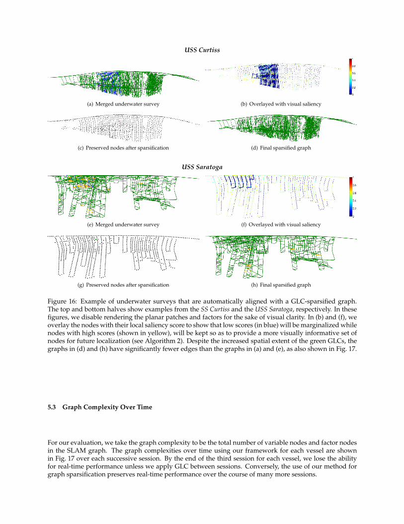
We performed the proposed multi-session SLAM on two vessels, USS Saratoga and SS Curtiss. In particular,the SS Curtiss was surveyed over a three year period as shown in Table 1. While the current mission exe-cutes, it is localized to a GLC-sparsified graph using Algorithm 1. Examples of matches using this approachare shown in Fig. 14. Though the algorithm shows some resilience to lighting, sunlight, and shadows, thisis not always the case (see Fig. 15 for one such example). In total, eight missions on USS Saratoga andtwelve missions on SS Curtiss are merged as in Fig. 16. These missions are accumulated into a commonhull-relative reference frame, and sparsified after each session. The end result is a far more extensive mapof each ship hull, as compared to the single session case.
USS Curtiss
(a) Merged underwater survey (b) Overlayed with visual saliency
(c) Preserved nodes after sparsification (d) Final sparsified graph
USS Saratoga
(e) Merged underwater survey (f) Overlayed with visual saliency
(g) Preserved nodes after sparsification (h) Final sparsified graph
Figure 16: Example of underwater surveys that are automatically aligned with a GLC-sparsified graph.The top and bottom halves show examples from the SS Curtiss and the USS Saratoga, respectively. In thesefigures, we disable rendering the planar patches and factors for the sake of visual clarity. In (b) and (f), weoverlay the nodes with their local saliency score to show that low scores (in blue) will be marginalized whilenodes with high scores (shown in yellow), will be kept so as to provide a more visually informative set ofnodes for future localization (see Algorithm 2). Despite the increased spatial extent of the green GLCs, thegraphs in (d) and (h) have significantly fewer edges than the graphs in (a) and (e), as also shown in Fig. 17.
5.3 Graph Complexity Over Time
For our evaluation, we take the graph complexity to be the total number of variable nodes and factor nodesin the SLAM graph. The graph complexities over time using our framework for each vessel are shownin Fig. 17 over each successive session. By the end of the third session for each vessel, we lose the abilityfor real-time performance unless we apply GLC between sessions. Conversely, the use of our method forgraph sparsification preserves real-time performance over the course of many more sessions.

1 2 3 4 5 6 7 8Session ID
0
1
2
3
4
5
6
7×10⁴
Node count, full
Factor count, full
Node count, GLC
Factor count, GLC
(a) USS Saratoga
2 4 6 8 10 12Session ID
0.0
0.2
0.4
0.6
0.8
1.0
1.2
1.4
1.6×10⁵
Node count, full
Factor count, full
Node count, GLC
Factor count, GLC
(b) SS Curtiss
Figure 17: Graph complexity over multiple sessions for the USS Saratoga, in (a), and the SS Curtiss, in (b).Without managing the graph complexity, the number of nodes and factors grows unbounded with time.However, the size of the graph using the GLC framework is much more closely bounded to the size of theship hull. For the USS Saratoga, sessions 1 through 7 occur within a week of each other, but session 8 occursfour months later. For the SS Curtiss, sessions 5 through 12 occur approximately three years after sessions1 through 4.
Algorithm 3 Match current keyframe to feasible keyframes from visual place-recognition system
1: Input: Set of all keyframes, K, in GLC-sparsified graph, current keyframe k, belief threshold τ , ship-specificvocabulary, V
2: S← FAB-MAPV2(k, K, V, τ )3: Output: FINDBESTMATCH(k, S) ⊲ Uses GPU
5.4 Comparison to Bag-of-Words Place Recognition
To baseline the performance of our particle filter, we use an open-source implementation of FAB-MAPversion 2.0 (Glover et al., 2012) as an appearance-only method for place recognition, which representseach keyframe as a visual BoW using a vocabulary that is learned offline. This algorithm is summarizedin Algorithm 3, and can be used in place of Algorithm 1 for initial alignment. FAB-MAP provides the beliefthat the live image is taken from the same location as a place in a prior map. If a match is detected withsignificant probability, a threshold is used to determine if the SLAM front-end should accept the match.This threshold is typically set very high to avoid false-positives, but we use a very low threshold of 0.0001for our application to ensure that FAB-MAP returns as many candidates as possible. These candidates aregeometrically verified using RANSAC in the final step to reject outliers.
For FAB-MAP, we learn a separate SIFT vocabulary and CLT over the distribution of codewords for eachvessel. In practice, this is impractical because it requires a training stage before multi-session SLAM canbe attempted. Even so, based upon our experiments, FAB-MAP’s performance is acceptable when match-ing images of the ship’s above-water superstructure, like the ones shown in Fig. 14(a) or Fig. 18, top row.However, for the underwater images, FAB-MAP performs poorly, and we were not able to successfullyidentify an underwater loop-closure in any of our experiments, even with a very low loop-closure prob-ability threshold. For underwater images, FAB-MAP consistently identifies the live underwater image asbeing taken from an unseen place. Two typical cases for the periscope and underwater cameras are shownvisually in Fig. 18.

Figure 18: Two representative attempts at aligning the current survey into past sessions using FAB-MAPand our particle filter. Corresponding image regions, where identified, are highlighted. We allow FAB-MAPto return as many candidates as possible by setting the loop-closure probability threshold low. By contrast,the number of candidate matches identified by our particle filter depends on how discriminative the planarmeasurements are. Because the image matching algorithm is done on the GPU, each candidate match takesroughly 70 ms when using a consumer-grade GPU. FAB-MAP performs adequately for surveys consistingof periscope images (top row) but fails using underwater images (bottom row), where it consistently assignsthe “new place” label.
Table 2: Time to localize to past GLC graph
Time until alignment (sec)
Session FAB-MAP Particle Filter Search
USS Saratoga 2013 Session 7, starting from surface 7.1 5.2USS Saratoga 2013 Session 7, starting underwater 143.2 20.6SS Curtiss 2011 Session 12, underwater-only N/A 15.3
Where our method excels over FAB-MAP is the ability re-localize into a previous session while underwater.We consider three scenarios: i) starting the survey with the robot at the surface, ii) starting submerged,and iii) a survey conducted entirely underwater. The results summarized in Table 2 are as follows: bothmethods are comparable when at the surface (first row), but FAB-MAP is unable to re-localize while startingunderwater, and only when the robot surfaces can it find a good match (second row). For an entirelyunderwater survey (third row), FAB-MAP is unable to localize. As a whole, our system, which is tailoredfor the sensor payload of the HAUV, can more quickly and reliably localize to our long-term SLAM graphs.
Using either the particle filter or FAB-MAP, we strive to keep the recall of candidate images as high aspossible. Reasonably low precision is not a primary concern because we can geometrically verify candi-date matches relatively quickly. If we compute the precision and recall of the set S from particle filtering(Algorithm 1) and FAB-MAP (Algorithm 3), we find that the particle filter produces a set of candidate im-ages with a lower average precision of 3.0%, but high average recall of 100.0%. FAB-MAP, on the otherhand, produces a higher average precision of 12.1%, but a much lower average recall of only 27.7%. Inother words, the particle filter always contains the correct place within the candidate set, but requires ge-ometrically verifying more keyframes. With FAB-MAP, the candidate set is smaller and therefore faster toprocess, however, localization will often fail because a true match is not contained in the set of candidateimages.
5.5 Comparison to Full Graph
To assess the accuracy of the GLC-based marginalization tool, we tracked the graph produced by the re-peated application of sparse-approximate GLC after each session is completed. This graph was directlycompared to a synthetically-created full graph, with no marginalized nodes, that contains the exact set ofmeasurements that the HAUV accumulated over the course of each session. For the SS Curtiss, we showthe full graph over all twelve sessions reported in this paper in Fig. 19.
These comparisons are shown in Fig. 20 for the USS Saratoga and in Fig. 21 for the SS Curtiss. Each measureis computed only for the vehicle pose nodes for sake of clarity. For each session, we compute the following:(i) marginal Kullback-Leibler Divergence (KLD) over each node (a measure of the similarity between twoprobability distributions), (ii) absolute positional distance between each corresponding node, (iii) absoluteattitude difference between each node, defined as the l2-norm of the difference of the poses’ Euler angles,and (iv) ratio of the determinants of marginal covariances of each node. For the KLD calculation, we usethe well-known closed-form expression for KLD between two Gaussian distributions (Kullback and Leibler,1951).
As a whole, the accuracy of our system is quite comparable to the full graph, showing typical errors wellwithin a meter despite a total path length of multiple kilometers. These errors are absolute, however,and they do not take into account the strong correlations between neighborhoods of nodes. In addition, asshown in Fig. 22, the marginal ellipses of the approximated poses are consistent with the full graph. Thoughrepeated sparsification may eventually result in inconsistent estimates, recent works include Carlevaris-Bianco and Eustice (2013b, 2014), which can guarantee that the GLC approximation is conservative tocounter these inconsistencies. Seeing how these methods affect the success rate of data association is aninteresting topic that remains to be explored. For the long-term datasets covered here, inconsistent approx-imations were not an issue; we were able to successfully establish camera measurements across multiplesessions throughout the field trials.
5.6 Importance of Planar Constraints and Comparison to CAD Model
We provide some qualitative results in Fig. 23 to show that the effectiveness of the method depends stronglyon the use of planar constraints. In this figure, we disabled both the piecewise-planar factor potentialfrom (3) and the planar range factors from (4). To keep the comparison fair, we provided the same particlefilter localizations used in Fig. 19.
Additionally, we used the ground truth CAD model to assess the quality of the SLAM trajectory, with andwithout planar constraints. We converted the DVL range returns into a global-frame point cloud usingthe estimated SLAM poses and down-sampled them with voxel grid filter. Then, we rigidly aligned thesepoints to the CAD mesh with generalized iterative closest point (GICP) (Segal et al., 2009). Finally, for eachpoint in the DVL point cloud we found the nearest vertex in the CAD mesh and computed the Euclideandistance.
This method serves as a sufficient proxy for the structural consistency of the SLAM estimate as comparedto ground truth. The results of this comparison are shown in Fig. 24. For the SLAM estimate with no planarconstraints, the error distribution had a mean of 1.31 m and standard deviation of 1.38 m. Furthermore,20% of the DVL points had an error of more than 1.5 m.
Conversely, the use of planar constraints brought the mean and standard deviation to 0.45 m and 0.19 m,respectfully. In addition, there were no points that had an error of more than 1.5 m. With these results, weconclude that camera constraints alone are not sufficient for long-term hull inspection, and we have shownthat the results are greatly improved if the ship hull surface itself is included in the SLAM pipeline.

(a) Full graph, side (b) Full graph, bottom
(c) GLC graph, side (d) GLC graph, bottom
Figure 19: The full, unsparsified graph of the SS Curtiss after twelve automatically-aligned sessions thatspans from February, 2011 to March, 2014. The CAD model is aligned to provide visual clarity and sizereference — it is not used in the SLAM system. The non-sparsified factor graphs in (a) and (b) consist ofodometry factors (blue), camera links (red), piecewise-planar factors from (3) (yellow), and planar rangefactors from (5) (lime green). The sparsified graphs in (c) and (d) consist mostly of GLC factors (green).These graphs serve as the comparison for the results in Fig. 21 for SessionID = 12.
6 Conclusion
We provided an overview of how to adapt our visual SLAM algorithm for long-term use on large shiphulls. We use the GLC framework to remove redundant or unneeded nodes from a factor graph. Doing soinvolves supporting a node reparameterization (root-shift) operation to avoid unnecessary error inducedby world-frame linearization. Furthermore, we described a particle filtering algorithm that can use planarsurface measurements to narrow a search space over past images that match the current image.
We showed results from our localization algorithm automatically aligning SLAM sessions separated intime by days, months, and years. Once sessions were aligned to a past graph, the result was sparsified andthe process was repeated. Using simple sparsification criteria, we show that the complexity of our factorgraphs remain more closely bounded to the ship hull area, rather than growing unbounded with time.Furthermore, despite the repeated applications of graph sparsification with GLC, the errors between thesparsified and non-sparsified graphs are reasonably small.

1 2 3 4 5 6 7 8Session ID
0.0
0.1
0.2
0.3
0.4
0.5
0.6
0.7
0.8
0.9P
ositio
nalerr
or
(m)
0.0
0.5
1.0
1.5
2.0
2.5
3.0
Tota
ltr
aje
cto
ryle
ngth
(km
)
(a) Positional Error
1 2 3 4 5 6 7 8Session ID
0.0
0.1
0.2
0.3
0.4
0.5
0.6
0.7
0.8
Attitude
err
or
(degre
es)
(b) Attitude Error
1 2 3 4 5 6 7 8
Session ID
0.0
0.1
0.2
0.3
0.4
0.5
0.6
Marg
inalK
LD
(nats
)
(c) KL Divergence
1 2 3 4 5 6 7 8Session ID
−2.0
−1.5
−1.0
−0.5
0.0
0.5
1.0
log( Σ
GLC
ii/Σ
Full
ii
)
(d) log(
ΣGLCii
/ΣFullii
)
Figure 20: Positional error and trajectory length (a), attitude error (b), average KLD (c), and log-ratio ofmarginal covariances (d) as a timeseries for the 2014 USS Saratoga datasets. The average value is shown assolid blue line. Percentile bounds are shown in the shaded region, from 5% to 95%.
2 4 6 8 10 12Session ID
0.0
0.1
0.2
0.3
0.4
0.5
0.6
Positio
nalerr
or
(m)
0
1
2
3
4
5
6
7
8
Tota
ltr
aje
cto
ryle
ngth
(km
)
(a) Positional Error
2 4 6 8 10 12Session ID
0.0
0.1
0.2
0.3
0.4
0.5
0.6
0.7
Attitude
err
or
(degre
es)
(b) Attitude Error
2 4 6 8 10 12
Session ID
0.0
0.2
0.4
0.6
0.8
1.0
1.2
1.4
Marg
inalK
LD
(nats
)
(c) KL Divergence
2 4 6 8 10 12Session ID
−1.5
−1.0
−0.5
0.0
0.5
1.0
log( Σ
GLC
ii/Σ
Full
ii
)
(d) log(
ΣGLCii
/ΣFullii
)
Figure 21: Comparisons to the full graph for each session for the SS Curtiss datasets. We show positionalerror (a), attitude error (b), average KLD (c), and log-ratio of marginal covariances (d) as a timeseries. Theaverage value is shown as solid blue line. Percentile bounds are shown in the shaded region, from 5% to95%.
−30 −25 −20 −15 −10 −5y (m)
−20
−15
−10
−5
0
x(m
)
Full
GLC (CLT)
(a) USS Saratoga
−35 −30 −25 −20 −15y (m)
−20
−15
−10
−5
x(m
)
Full
GLC (CLT)
(b) SS Curtiss
Figure 22: Visualizations of 3-σ positional covariances for the full graph are shown in red, and the cor-responding ellipses from the GLC-sparsified graph are shown in blue. Our system marginalizes approx-imately 95% of nodes from each session so that the system can perform in real-time, yet the probabilisticdeviation from the full graph is small. The results for the USS Saratoga and SS Curtiss are shown in (a)and (b), respectively.
Acknowledgments
This work was supported by the Office of Naval Research under award N00014-12-1-0092.

(a) Full graph, side (b) Full graph,bottom
Figure 23: The quality of the SLAM estimate suffers significantly if the planar-based constraints from §3.4.2and §3.4.3 are left out of the factor graph. These constraints are encoded as yellow and green linesin Fig. 19(a). The CAD model is once again provided for visual reference, and to show that there are obviousdiscrepancies between it and the SLAM estimate. These discrepancies are quantified in Fig. 24.
(a) DVL alignment with planar constraints (b) DVL alignment without planar constraints
0 1 2 3 4 5 6 7 8Error (m)
0.0
0.1
0.2
0.3
0.4
0.5
0.6
Rela
tive
frequency
W/out planar const.
W/ planar const.
(c) Error histogram for (a) and (b)
Figure 24: For the SS Curtiss, we were able to quantify the error with respect to the ground truth CAD modelby registering the DVL returns (red and blue point clouds) to the CAD mesh vertices (gray point cloud).The DVL point cloud in (a) was derived from the SLAM estimate in Fig. 19 (with planar constraints), whilethe point cloud in (b) was derived from Fig. 23 (without planar constraints). The Euclidean error betweencorresponding vertices in the CAD model mesh is summarized in (c), where the planar constraints providea much tighter distribution of error.

A Appendix
A.1 Spherical to Cartesian Coordinates
The characteristic curvature model used in this paper lends itself to surface normals expressed in sphericalcoordinates. To convert the xyz normal vector to a stacked vector of normal azimuth, a, elevation, e, andmagnitude, m, we use the dir( · ) function:
dir
xyz
=
atan2(y, x)
atan2(z,√x2 + y2
)√x2 + y2 + z2
.
Similarly, to convert from spherical coordinates back to Cartesian, we use the trans( · ) function, defined as:
trans
aem
= m
cos(e) cos(a)cos(e) sin(a)
sin(e)
.
References
Agarwal, P., Tipaldi, G. D., Spinello, L., Stachniss, C., and Burgard, W. (2013). Robust map optimizationusing dynamic covariance scaling. In Proceedings of the IEEE International Conference on Robotics and Au-tomation, pages 62–69, Karlsruhe, Germany.
Bay, H., Tuytelaars, T., and Van Gool, L. (2006). SURF: Speeded up robust features. In Proceedings of theEuropean Conference on Computer Vision, pages 404–417, Graz, Austria. Springer.
Belcher, E., Matsuyama, B., and Trimble, G. (2001). Object identification with acoustic lenses. In Proceedingsof the IEEE/MTS OCEANS Conference and Exhibition, volume 1, pages 6–11, Kona, HI, USA.
Bonnın-Pascual, F. and Ortiz, A. (2010). Detection of cracks and corrosion for automated vessels visualinspection. In Proceedings of the International Conference of the Catalan Association for Artificial Intelligence,pages 111–120, Tarragona, Spain.
Boon, B., Brennan, F., Garbatov, Y., Ji, C., Parunov, J., Rahman, T., Rizzo, C., Rouhan, A., Shin, C., andYamamoto, N. (2009). Condition assessment of aged ships and offshore structures. In International Shipand Offshore Structures Congress, volume 2, pages 313–365, Seoul, Korea.
Bosse, M., Newman, P., Leonard, J., and Teller, S. (2004). Simultaneous localization and map buildingin large-scale cyclic environments using the Atlas framework. International Journal of Robotics Research,23(12):1113–1139.
Bosse, M. and Zlot, R. (2008). Map matching and data association for large-scale two-dimensional laserscan-based SLAM. International Journal of Robotics Research, 27(6):667–691.
Bowen, A. D., Yoerger, D. R., Taylor, C., McCabe, R., Howland, J., Gomez-Ibanez, D., Kinsey, J. C., Heintz,M., McDonald, G., Peters, D. B., Bailey, J., Bors, E., Shank, T., Whitcomb, L. L., Martin, S. C., Webster,S. E., Jakuba, M. V., Fletcher, B., Young, C., Buescher, J., Fryer, P., and Hulme, S. (2009). Field trials of theNereus hybrid underwater robotic vehicle in the challenger deep of the Mariana Trench. In Proceedings ofthe IEEE/MTS OCEANS Conference and Exhibition, pages 1–10, Biloxi, MS, USA.
Carlevaris-Bianco, N. and Eustice, R. M. (2011). Multi-view registration for feature-poor underwater im-agery. In Proceedings of the IEEE International Conference on Robotics and Automation, pages 423–430, Shang-hai, China.
Carlevaris-Bianco, N. and Eustice, R. M. (2013a). Generic factor-based node marginalization and edgesparsification for pose-graph SLAM. In Proceedings of the IEEE International Conference on Robotics andAutomation, pages 5728–5735, Karlsruhe, Germany.

Carlevaris-Bianco, N. and Eustice, R. M. (2013b). Long-term simultaneous localization and mapping withgeneric linear constraint node removal. In Proceedings of the IEEE/RSJ International Conference on IntelligentRobots and Systems, pages 1034–1041, Tokyo, Japan.
Carlevaris-Bianco, N. and Eustice, R. M. (2014). Conservative edge sparsification for graph SLAM noderemoval. In Proceedings of the IEEE International Conference on Robotics and Automation, pages 854–860,Hong Kong, China.
Carvalho, A., Sagrilo, L., Silva, I., Rebello, J., and Carneval, R. (2003). On the reliability of an automatedultrasonic system for hull inspection in ship-based oil production units. Applied Ocean Research, 25(5):235–241.
Cummins, M. and Newman, P. (2008). FAB-MAP: Probabilistic localization and mapping in the space ofappearance. International Journal of Robotics Research, 27(6):647–665.
Dellaert, F. and Kaess, M. (2006). Square root SAM: Simultaneous localization and mapping via square rootinformation smoothing. International Journal of Robotics Research, 25(12):1181–1203.
Eade, E., Fong, P., and Munich, M. (2010). Monocular graph SLAM with complexity reduction. In Pro-ceedings of the IEEE/RSJ International Conference on Intelligent Robots and Systems, pages 3017–3024, Taipei,Taiwan.
Eustice, R. M., Pizarro, O., and Singh, H. (2008). Visually augmented navigation for autonomous underwa-ter vehicles. IEEE Journal of Ocean Engineering, 33(2):103–122.
Glover, A., Maddern, W., Warren, M., Reid, S., Milford, M., and Wyeth, G. (2012). OpenFABMAP: Anopen source toolbox for appearance-based loop closure detection. In Proceedings of the IEEE InternationalConference on Robotics and Automation, pages 4730–4735, St. Paul, USA.
Grisetti, G., Stachniss, C., Grzonka, S., and Burgard, W. (2007). A tree parameterization for efficientlycomputing maximum likelihood maps using gradient descent. In Proceedings of the Robotics: Science &Systems Conference, pages 65–72, Atlanta, GA, USA.
Gustafson, E., Jalving, B., ystein Engelhardtsen, and Burchill, N. (2011). HUGIN 1000 Arctic class AUV. InThe Polar Petroleum Potential Conference & Exhibition, pages 714–721, Halifax, Nova Scotia.
Harris, S. and Slate, E. (1999). Lamp ray: Ship hull assessment for value, safety and readiness. In Proceedingsof the IEEE/MTS OCEANS Conference and Exhibition, volume 1, pages 493–500, Seattle, WA, USA.
Hover, F., Vaganay, J., Elkins, M., Willcox, S., Polidoro, V., Morash, J., Damus, R., and Desset, S. (2007).A vehicle system for autonomous relative survey of in-water ships. Marine Technology Society Journal,41(2):44–55.
Hover, F. S., Eustice, R. M., Kim, A., Englot, B., Johannsson, H., Kaess, M., and Leonard, J. J. (2012). Ad-vanced perception, navigation and planning for autonomous in-water ship hull inspection. InternationalJournal of Robotics Research, 31(12):1445–1464.
Ishizu, K., Sakagami, N., Ishimaru, K., Shibata, M., Onishi, H., Murakami, S., and Kawamura, S. (2012). Shiphull inspection using a small underwater robot with a mechanical contact mechanism. In Proceedings ofthe IEEE/MTS OCEANS Conference and Exhibition, pages 1–6, Hampton Roads, VA, USA.
Johannsson, H., Kaess, M., Englot, B., Hover, F., and Leonard, J. J. (2010). Imaging sonar-aided navigationfor autonomous underwater harbor surveillance. In Proceedings of the IEEE/RSJ International Conference onIntelligent Robots and Systems, pages 4396–4403, Taipei, Taiwan.
Julier, S. (2002). The scaled unscented transformation. In Proceedings of the American Control Conference,volume 6, pages 4555–4559, Anchorage, AK, USA.
Kaess, M. and Dellaert, F. (2009). Covariance recovery from a square root information matrix for dataassociation. Robotics and Autonomous Systems, 57(12):1198–1210.
Kaess, M., Johannsson, H., Rosen, D., Carlevaris-Bianco, N., and Leonard, J. (2010). Open source imple-mentation of iSAM. http://people.csail.mit.edu/kaess/isam.
Kaess, M., Ranganathan, A., and Dellaert, F. (2008). iSAM: Incremental smoothing and mapping. IEEETransactions on Robotics, 24(6):1365–1378.

Kim, A. and Eustice, R. M. (2009). Pose-graph visual SLAM with geometric model selection for autonomousunderwater ship hull inspection. In Proceedings of the IEEE/RSJ International Conference on Intelligent Robotsand Systems, pages 1559–1565, St. Louis, MO, USA.
Kim, A. and Eustice, R. M. (2013). Real-time visual SLAM for autonomous underwater hull inspectionusing visual saliency. IEEE Transactions on Robotics, 29(3):719–733.
Kim, B., Kaess, M., Fletcher, L., Leonard, J., Bachrach, A., Roy, N., and Teller, S. (2010). Multiple relativepose graphs for robust cooperative mapping. In Proceedings of the IEEE International Conference on Roboticsand Automation, pages 3185–3192, Anchorage, AK, USA.
Konolige, K. and Bowman, J. (2009). Towards lifelong visual maps. In Proceedings of the IEEE/RSJ Interna-tional Conference on Intelligent Robots and Systems, pages 1156–1163, St. Louis, MO, USA.
Kretzschmar, H. and Stachniss, C. (2012). Information-theoretic compression of pose graphs for laser-basedSLAM. International Journal of Robotics Research, 31(11):1219–1230.
Kullback, S. and Leibler, R. A. (1951). On information and sufficiency. The Annals of Mathematical Statistics,22(1):79–86.
Kummerle, R., Grisetti, G., Strasdat, H., Konolige, K., and Burgard, W. (2011). g2o: A general framework forgraph optimization. In Proceedings of the IEEE International Conference on Robotics and Automation, pages3607–3613, Shanghai, China.
Kunz, C., Murphy, C., Singh, H., Pontbriand, C., Sohn, R. A., Singh, S., Sato, T., Roman, C., Nakamura, K.-i.,Jakuba, M., Eustice, R., Camilli, R., and Bailey, J. (2009). Toward extraplanetary under-ice exploration:Robotic steps in the arctic. Journal of Field Robotics, 26(4):411–429.
Leonard, J. and Feder, H. (1999). A computationally efficient method for large-scale concurrent mappingand localization. In J., H. and Koditschek, D., editors, Proceedings of the International Symposium on RoboticsResearch, Salt Lake City, Utah, USA.
Lowe, D. (2004). Distinctive image features from scale-invariant keypoints. International Journal of ComputerVision, 60(2):91–110.
Menegaldo, L. L., Ferreira, G., Santos, M. F., and Guerato, R. S. (2009). Development and navigation of amobile robot for floating production storage and offloading ship hull inspection. IEEE Transactions onIndustrial Electronics, 56(9):3717–3722.
Menegaldo, L. L., Santos, M., Ferreira, G. A. N., Siqueira, R. G., and Moscato, L. (2008). SIRUS: A mobilerobot for floating production storage and offloading (FPSO) ship hull inspection. In Proceedings of theIEEE International Workshop on Advanced Motion Control, pages 27–32, Trento, Italy.
Milne, P. (1983). Underwater acoustic positioning systems. Gulf Publishing Company, Houston.
Muja, M. and Lowe, D. G. (2009). Fast approximate nearest neighbors with automatic algorithm configura-tion. In International Conference on Computer Vision Theory and Application, pages 331–340, Lisboa, Portugal.
Negahdaripour, S. and Firoozfam, P. (2006). An ROV stereovision system for ship-hull inspection. IEEEJournal of Oceanic Engineering, 31(3):551–564.
Neira, J. and Tardos, J. (2001). Data association in stochastic mapping using the joint compatibility test.IEEE Transactions on Robotics and Automation, 17(6):890–897.
Ni, K., Steedly, D., and Dellaert, F. (2007). Tectonic SAM: Exact, out-of-core, submap-based SLAM. InProceedings of the IEEE International Conference on Robotics and Automation, pages 1678–1685, Roma, Italy.
Nister, D. and Stewenius, H. (2006). Scalable recognition with a vocabulary tree. In Proceedings of the IEEEConference on Computer Vision and Pattern Recognition, volume 2, pages 2161–2168.
Ozog, P. and Eustice, R. M. (2013a). On the importance of modeling camera calibration uncertainty in visualSLAM. In Proceedings of the IEEE International Conference on Robotics and Automation, pages 3762–3769,Karlsruhe, Germany.
Ozog, P. and Eustice, R. M. (2013b). Real-time SLAM with piecewise-planar surface models and sparse 3Dpoint clouds. In Proceedings of the IEEE/RSJ International Conference on Intelligent Robots and Systems, pages1042–1049, Tokyo, Japan.

Ozog, P. and Eustice, R. M. (2014). Toward long-term, automated ship hull inspection with visual SLAM,explicit surface optimization, and generic graph-sparsification. In Proceedings of the IEEE InternationalConference on Robotics and Automation, pages 3832–3839, Hong Kong, China.
Pizarro, O., Eustice, R. M., and Singh, H. (2009). Large area 3-D reconstructions from underwater opticalsurveys. IEEE Journal of Oceanic Engineering, 34(2):150–169.
Ridao, P., Carreras, M., Ribas, D., and Garcia, R. (2010). Visual inspection of hydroelectric dams using anautonomous underwater vehicle. Journal of Field Robotics, 27(6):759–778.
Roman, C. and Singh, H. (2005). Improved vehicle based multibeam bathymetry using sub-maps andSLAM. In Proceedings of the IEEE/RSJ International Conference on Intelligent Robots and Systems, pages 2422–2429, Edmonton, Alberta, Canada.
Segal, A., Haehnel, D., and Thrun, S. (2009). Generalized-ICP. In Proceedings of the Robotics: Science &Systems Conference, Seattle, WA, USA.
Singh, H., Armstrong, R., Gilbes, F., Eustice, R., Roman, C., Pizarro, O., and Torres, J. (2004). Imagingcoral I: Imaging coral habitats with the SeaBED AUV. The Journal for Subsurface Sensing Technologies andApplications, 5(1):25–42.
Smith, R., Self, M., and Cheeseman, P. (1986). Estimating uncertain spatial relationships in robotics. InProceedings of Uncertainty in AI, pages 267–288, Philadelphia, PA, USA. Elsevier.
Sunderhauf, N. and Protzel, P. (2012). Switchable constraints for robust pose graph SLAM. In Proceedings ofthe IEEE/RSJ International Conference on Intelligent Robots and Systems, pages 1879–1884, Algarve, Portugal.
Thrun, S. and Montemerlo, M. (2006). The graph SLAM algorithm with applications to large-scale mappingof urban structures. International Journal of Robotics Research, 25(5-6):403–429.
Trevor, A. J. B., Rogers, J. G., and Christensen, H. I. (2012). Planar surface SLAM with 3D and 2D sensors. InProceedings of the IEEE International Conference on Robotics and Automation, pages 3041–3048, St. Paul, MN,USA.
Trimble, G. and Belcher, E. (2002). Ship berthing and hull inspection using the CetusII AUV and MIRIShigh-resolution sonar. In Proceedings of the IEEE/MTS OCEANS Conference and Exhibition, volume 2, pages1172–1175, Biloxi, MS, USA.
VanMiddlesworth, M., Kaess, M., Hover, F., and Leonard, J. (2013). Mapping 3D underwater environmentswith smoothed submaps. In Proceedings of the International Conference on Field and Service Robotics, pages17–30, Brisbane, Australia.
Walter, M., Hover, F., and Leonard, J. (2008). SLAM for ship hull inspection using exactly sparse extendedinformation filters. In Proceedings of the IEEE International Conference on Robotics and Automation, pages1463–1470, Pasadena, CA, USA.
Weingarten, J. and Siegwart, R. (2006). 3D SLAM using planar segments. In Proceedings of the IEEE/RSJInternational Conference on Intelligent Robots and Systems, pages 3062–3067, Beijing, China.