Long short-term memory and learning-to-learn innetworks of spiking neurons

Guillaume Bellec*, Darjan Salaj*, Anand Subramoney*, Robert Legenstein & Wolfgang MaassInstitute for Theoretical Computer Science

Graz University of Technology, Austria{bellec,salaj,subramoney,legenstein,maass}@igi.tugraz.at

* equal contributions

Abstract

Recurrent networks of spiking neurons (RSNNs) underlie the astounding comput-ing and learning capabilities of the brain. But computing and learning capabilitiesof RSNN models have remained poor, at least in comparison with artificial neuralnetworks (ANNs). We address two possible reasons for that. One is that RSNNsin the brain are not randomly connected or designed according to simple rules,and they do not start learning as a tabula rasa network. Rather, RSNNs in thebrain were optimized for their tasks through evolution, development, and priorexperience. Details of these optimization processes are largely unknown. Buttheir functional contribution can be approximated through powerful optimizationmethods, such as backpropagation through time (BPTT).A second major mismatch between RSNNs in the brain and models is that thelatter only show a small fraction of the dynamics of neurons and synapses inthe brain. We include neurons in our RSNN model that reproduce one promi-nent dynamical process of biological neurons that takes place at the behaviourallyrelevant time scale of seconds: neuronal adaptation. We denote these networksas LSNNs because of their Long short-term memory. The inclusion of adaptingneurons drastically increases the computing and learning capability of RSNNs ifthey are trained and configured by deep learning (BPTT combined with a rewiringalgorithm that optimizes the network architecture). In fact, the computational per-formance of these RSNNs approaches for the first time that of LSTM networks.In addition RSNNs with adapting neurons can acquire abstract knowledge fromprior learning in a Learning-to-Learn (L2L) scheme, and transfer that knowledgein order to learn new but related tasks from very few examples. We demonstratethis for supervised learning and reinforcement learning.

1 Introduction

Recurrent networks of spiking neurons (RSNNs) are frequently studied as models for networks ofneurons in the brain. In principle, they should be especially well-suited for computations in thetemporal domain, such as speech processing, as their computations are carried out via spikes, i.e.,events in time and space. But the performance of RSNN models has remained suboptimal also fortemporal processing tasks. One difference between RSNNs in the brain and RSNN models is thatRSNNs in the brain have been optimized for their function through long evolutionary processes,complemented by a sophisticated learning curriculum during development. Since most details ofthese biological processes are currently still unknown, we asked whether deep learning is able tomimic these complex optimization processes on a functional level for RSNN models. We usedBPTT as the deep learning method for network optimization. Backpropagation has been adaptedpreviously for feed forward networks with binary activations in [1, 2], and we adapted BPTT to work

32nd Conference on Neural Information Processing Systems (NeurIPS 2018), Montreal, Canada.

in a similar manner for RSNNs. In order to also optimize the connectivity of RSNNs, we augmentedBPTT with DEEP R, a biologically inspired heuristic for synaptic rewiring [3, 4]. Compared toLSTM networks, RSNNs tend to have inferior short-term memory capabilities. Since neurons in thebrain are equipped with a host of dynamics processes on time scales larger than a few dozen ms [5],we enriched the inherent dynamics of neurons in our model by a standard neural adaptation process.

We first show (section 4) that this approach produces new computational performance levels ofRSNNs for two common benchmark tasks: Sequential MNIST and TIMIT (a speech processingtask). We then show that it makes L2L applicable to RSNNs (section 5), similarly as for LSTMnetworks. In particular, we show that meta-RL [6, 7] produces new motor control capabilities ofRSNNs (section 6). This result links a recent abstract model for reward-based learning in the brain[8] to spiking activity. In addition, we show that RSNNs with sparse connectivity and sparse firingactivity of 10-20 Hz (see Fig. 1D, 2D, S1C) can solve these and other tasks. Hence these RSNNscompute with spikes, rather than firing rates.

The superior computing and learning capabilities of LSNNs suggest that they are also of interest forimplementation in spike-based neuromorphic chips such as Brainscales [9], SpiNNaker [10], TrueNorth [2], chips from ETH Zurich [11], and Loihi [12]. In particular, nonlocal learning rules suchas backprop are challenges for some of these neuromorphic devices (and for many brain models).Hence alternative methods for RSNN learning of nonlinear functions are needed. We show in sec-tions 5 and 6 that L2L can be used to generate RSNNs that learn very efficiently even in the absenceof synaptic plasticity.

Relation to prior work: We refer to [13, 14, 15, 16] for summaries of preceding results on compu-tational capabilities of RSNNs. The focus there was typically on the generation of dynamic patterns.Such tasks are not addressed in this article, but it will be shown in [17] that LSNNs provide an al-ternative model to [16] for the generation of complex temporal patterns. Huh et al. [15] appliedgradient descent to recurrent networks of spiking neurons. There, neurons without a leak were used.Hence, the voltage of a neuron could used in that approach to store information over an unlimitedlength of time.

We are not aware of previous attempts to bring the performance of RSNNs for time series classifica-tion into the performance range of LSTM networks. We are also not aware of any previous literatureon applications of L2L to SNNs.

2 LSNN model

Neurons and synapses in common RSNN models are missing many of the dynamic processes foundin their biological counterparts, especially those on larger time scales. We integrate one of theminto our RSNN model: neuronal adaptation. It is well known that a substantial fraction of excita-tory neurons in the brain are adapting, with diverse time constants, see e.g. the Allen Brain Atlasfor data from the neocortex of mouse and humans. We refer to the resulting type of RSNNs asLong short-term memory Spiking Neural Networks (LSNNs). LSNNs consist of a population Rof integrate-and-fire (LIF) neurons (excitatory and inhibitory), and a second population A of LIFexcitatory neurons whose excitability is temporarily reduced through preceding firing activity, i.e.,these neurons are adapting (see Fig. 1C and Suppl.). Both populations R and A receive spike trainsfrom a populationX of external input neurons. Results of computations are read out by a populationY of external linear readout neurons, see Fig. 1C.

Common ways for fitting models for adapting neurons to data are described in [18, 19, 20, 21]. Weare using here the arguably simplest model: We assume that the firing threshold Bj(t) of neuron jincreases by some fixed amount β/τa,j for each spike of this neuron j, and then decays exponentiallyback to a baseline value b0j with a time constant τa,j . Thus the threshold dynamics for a discretetime step of δt = 1 ms reads as follows

Bj(t) = b0j + βbj(t), (1)

bj(t+ δt) = ρjbj(t) + (1− ρj)zj(t), (2)

where ρj = exp(− δtτa,j

) and zj(t) is the spike train of neuron j assuming values in {0, 1δt}. Note

that this dynamics of thresholds of adaptive spiking neurons is similar to the dynamics of the stateof context neurons in [22]. It generally suffices to place the time constant of adapting neurons intothe desired range for short-term memory (see Suppl. for specific values used in each experiment).

2

3 Applying BPTT with DEEP R to RSNNs and LSNNs

We optimize the synaptic weights, and in some cases also the connectivity matrix of an LSNN forspecific ranges of tasks. The optimization algorithm that we use, backpropagation through time(BPTT), is not claimed to be biologically realistic. But like evolutionary and developmental pro-cesses, BPTT can optimize LSNNs for specific task ranges. Backpropagation (BP) had already beenapplied in [1] and [2] to feedforward networks of spiking neurons. In these approaches, the gradientis backpropagated through spikes by replacing the non-existent derivative of the membrane potentialat the time of a spike by a pseudo-derivative that smoothly increases from 0 to 1, and then decaysback to 0. We reduced (“dampened”) the amplitude of the pseudo-derivative by a factor < 1 (seeSuppl. for details). This enhances the performance of BPTT for RSNNs that compute during largertime spans, that require backpropagation through several 1000 layers of an unrolled feedforwardnetwork of spiking neurons. A similar implementation of BPTT for RSNNs was proposed in [15]. Itis not yet clear which of these two versions of BPTT work best for a given task and a given network.

In order to optimize not only the synaptic weights of a RSNN but also its connectivity matrix, weintegrated BPTT with the biologically inspired [3] rewiring method DEEP R [4] (see Suppl. fordetails). DEEP R converges theoretically to an optimal network configuration by continuously up-dating the set of active connections [23, 3, 4].

4 Computational performance of LSNNs

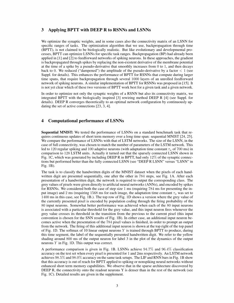
Sequential MNIST: We tested the performance of LSNNs on a standard benchmark task that re-quires continuous updates of short term memory over a long time span: sequential MNIST [24, 25].We compare the performance of LSNNs with that of LSTM networks. The size of the LSNN, in thecase of full connectivity, was chosen to match the number of parameters of the LSTM network. Thisled to 120 regular spiking and 100 adaptive neurons (with adaptation time constant τa of 700 ms) incomparison to 128 LSTM units. Actually it turned out that the sparsely connected LSNN shown inFig. 1C, which was generated by including DEEP R in BPTT, had only 12% of the synaptic connec-tions but performed better than the fully connected LSNN (see “DEEP R LSNN” versus “LSNN” inFig. 1B).

The task is to classify the handwritten digits of the MNIST dataset when the pixels of each hand-written digit are presented sequentially, one after the other in 784 steps, see Fig. 1A. After eachpresentation of a handwritten digit, the network is required to output the corresponding class. Thegrey values of pixels were given directly to artificial neural networks (ANNs), and encoded by spikesfor RSNNs. We considered both the case of step size 1 ms (requiring 784 ms for presenting the in-put image) and 2 ms (requiring 1568 ms for each image, the adaptation time constant τa was set to1400 ms in this case, see Fig. 1B.). The top row of Fig. 1D shows a version where the grey value ofthe currently presented pixel is encoded by population coding through the firing probability of the80 input neurons. Somewhat better performance was achieved when each of the 80 input neuronsis associated with a particular threshold for the grey value, and this input neuron fires whenever thegrey value crosses its threshold in the transition from the previous to the current pixel (this inputconvention is chosen for the SNN results of Fig. 1B). In either case, an additional input neuron be-comes active when the presentation of the 784 pixel values is finished, in order to prompt an outputfrom the network. The firing of this additional input neuron is shown at the top right of the top panelof Fig. 1D. The softmax of 10 linear output neurons Y is trained through BPTT to produce, duringthis time segment, the label of the sequentially presented handwritten digit. We refer to the yellowshading around 800 ms of the output neuron for label 3 in the plot of the dynamics of the outputneurons Y in Fig. 1D. This output was correct.

A performance comparison is given in Fig. 1B. LSNNs achieve 94.7% and 96.4% classificationaccuracy on the test set when every pixel is presented for 1 and 2ms respectively. An LSTM networkachieves 98.5% and 98.0% accuracy on the same task setups. The LIF and RNN bars in Fig. 1B showthat this accuracy is out of reach for BPTT applied to spiking or nonspiking neural networks withoutenhanced short term memory capabilities. We observe that in the sparse architecture discovered byDEEP R, the connectivity onto the readout neurons Y is denser than in the rest of the network (seeFig. 1C). Detailed results are given in the supplement.

3

Figure 1: Sequential MNIST. A The task is to classify images of handwritten digits when thepixels are shown sequentially pixel by pixel, in a fixed order row by row. B The performanceof RSNNs is tested for three different setups: without adapting neurons (LIF), a fully connectedLSNN, and an LSNN with randomly initialized connectivity that was rewired during training (DEEPR LSNN). For comparison, the performance of two ANNs, a fully connected RNN and an LSTMnetwork are also shown. C Connectivity (in terms of connection probabilities between and withinthe 3 subpopulations) of the LSNN after applying DEEP R in conjunction with BPTT. The inputpopulation X consisted of 60 excitatory and 20 inhibitory neurons. Percentages on the arrows fromX indicate the average connection probabilities from excitatory and inhibitory neurons. D Dynamicsof the LSNN after training when the input image from A was sequentially presented. From top tobottom: spike rasters from input neurons (X), and random subsets of excitatory (E) and inhibitory (I)regularly spiking neurons, and adaptive neurons (A), dynamics of the firing thresholds of a randomsample of adaptive neurons; activation of softmax readout neurons.

Speech recognition (TIMIT): We also tested the performance of LSNNs for a real-world speechrecognition task, the TIMIT dataset. A thorough study of the performance of many variations ofLSTM networks on TIMIT has recently been carried out in [26]. We used exactly the same setupwhich was used there (framewise classification) in order to facilitate comparison. We found thata standard LSNN consisting of 300 regularly firing (200 excitatory and 100 inhibitory) and 100excitatory adapting neurons with an adaptation time constant of 200 ms, and with 20% connectionprobability in the network, achieved a classification error of 33.2%. This error is below the meanerror around 40% from 200 trials with different hyperparameters for the best performing (and mostcomplex) version of LSTMs according to Fig. 3 of [26], but above the mean of 29.7% of the 20best performing choices of hyperparameters for these LSTMs. The performance of the LSNN washowever somewhat better than the error rates achieved in [26] for a less complex version of LSTMswithout forget gates (mean of the best 20 trials: 34.2%).

We could not perform a similarly rigorous search over LSNN architectures and meta-parametersas was carried out in [26] for LSTMs. But if all adapting neurons are replaced by regularly firingexcitatory neurons one gets a substantially higher error rate than the LSNN with adapting neurons:37%. Details are given in the supplement.

4

5 LSNNs learn-to-learn from a teacher

One likely reason why learning capabilities of RSNN models have remained rather poor is that oneusually requires a tabula rasa RSNN model to learn. In contrast, RSNNs in the brain have beenoptimized through a host of preceding processes, from evolution to prior learning of related tasks,for their learning performance. We emulate a similar training paradigm for RSNNs using the L2Lsetup. We explore here only the application of L2L to LSNNs, but L2L can also be applied toRSNNs without adapting neurons [27]. An application of L2L to LSNNs is tempting, since L2Lis most commonly applied in machine learning to their ANN counterparts: LSTM networks seee.g. [6, 7]. LSTM networks are especially suited for L2L since they can accommodate two levelsof learning and representation of learned insight: Synaptic connections and weights can encode,on a higher level, a learning algorithm and prior knowledge on a large time-scale. The short-termmemory of an LSTM network can accumulate, on a lower level of learning, knowledge during thecurrent learning task. It has recently been argued [8] that the pre-frontal cortex (PFC) similarlyaccumulates knowledge during fast reward-based learning in its short-term memory, without usingdopamine-gated synaptic plasticity, see the text to Suppl. Fig. 3 in [8]. The experimental results of[28] suggest also a prominent role of short-term memory for fast learning in the motor cortex.

The standard setup of L2L involves a large, in fact in general infinitely large, family F of learningtasks C. Learning is carried out simultaneously in two loops (see Fig. 2A). The inner loop learninginvolves the learning of a single task C by a neural network N , in our case by an LSNN. Someparameters of N (termed hyper-parameters) are optimized in an outer loop optimization to supportfast learning of a randomly drawn task C from F . The outer loop training – implemented herethrough BPTT – proceeds on a much larger time scale than the inner loop, integrating performanceevaluations from many different tasks C of the family F . One can interpret this outer loop asa process that mimics the impact of evolutionary and developmental optimization processes, aswell as prior learning, on the learning capability of brain networks. We use the terms training andoptimization interchangeably, but the term training is less descriptive of the longer-term evolutionaryprocesses we mimic. Like in [29, 6, 7] we let all synaptic weights of N belong to the set of hyper-parameters that are optimized through the outer loop. Hence the network is forced to encode allresults from learning the current task C in its internal state, in particular in its firing activity andthe thresholds of adapting neurons. Thus the synaptic weights of the neural network N are free toencode an efficient algorithm for learning arbitrary tasks C from F .

When the brain learns to predict sensory inputs, or state changes that result from an action, thiscan be formalized as learning from a teacher (i.e., supervised learning). The teacher is in this casethe environment, which provides – often with some delay – the target output of a network. TheL2L results of [29] show that LSTM networks can learn nonlinear functions from a teacher withoutmodifying their synaptic weights, using their short-term memory instead. We asked whether thisform of learning can also be attained by LSNNs.

Task: We considered the task of learning complex non-linear functions from a teacher. Specifically,we chose as family F of tasks a class of continuous functions of two real-valued variables (x1, x2).This class was defined as the family of all functions that can be computed by a 2-layer artificialneural network of sigmoidal neurons with 10 neurons in the hidden layer, and weights and biasesfrom [-1, 1], see Fig. 2B. Thus overall, each such target network (TN) from F was defined through40 parameters in the range [-1, 1]: 30 weights and 10 biases. We gave the teacher input to the LSNNfor learning a particular TN C from F in a delayed manner as in [29]: The target output value wasgiven after N had provided its guessed output value for the preceding input.

This delay of the feedback is consistent with biologically plausible scenarios. Simultaneously, hav-ing a delay for the feedback prevents N from passing on the teacher value as output without firstproducing a prediction on its own.

Implementation: We considered a LSNNN consisting of 180 regularly firing neurons (populationR) and 120 adapting neurons (population A) with a spread of adaptation time constants sampleduniformly between 1 and 1000 ms and with full connectivity. Sparse connectivity in conjunctionwith rewiring did not improve performance in this case. All neurons in the LSNN received inputfrom a populationX of 300 external input neurons. A linear readout received inputs from all neuronsin R and A. The LSNN received a stream of 3 types of external inputs (see top row of Fig. 2D): thevalues of x1, x2, and of the output C(x′1, x

′2) of the TN for the preceding input pair x′1, x

′2 (set to 0

5

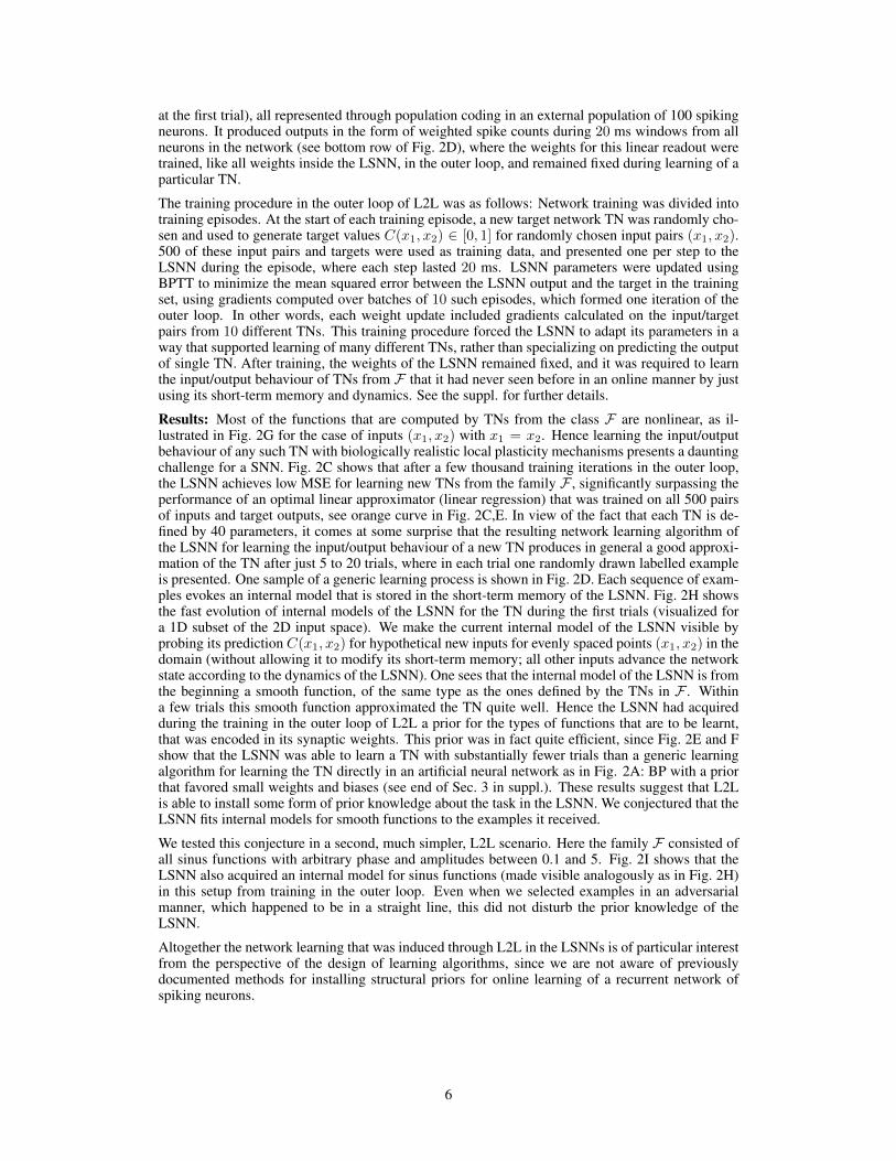
at the first trial), all represented through population coding in an external population of 100 spikingneurons. It produced outputs in the form of weighted spike counts during 20 ms windows from allneurons in the network (see bottom row of Fig. 2D), where the weights for this linear readout weretrained, like all weights inside the LSNN, in the outer loop, and remained fixed during learning of aparticular TN.

The training procedure in the outer loop of L2L was as follows: Network training was divided intotraining episodes. At the start of each training episode, a new target network TN was randomly cho-sen and used to generate target values C(x1, x2) ∈ [0, 1] for randomly chosen input pairs (x1, x2).500 of these input pairs and targets were used as training data, and presented one per step to theLSNN during the episode, where each step lasted 20 ms. LSNN parameters were updated usingBPTT to minimize the mean squared error between the LSNN output and the target in the trainingset, using gradients computed over batches of 10 such episodes, which formed one iteration of theouter loop. In other words, each weight update included gradients calculated on the input/targetpairs from 10 different TNs. This training procedure forced the LSNN to adapt its parameters in away that supported learning of many different TNs, rather than specializing on predicting the outputof single TN. After training, the weights of the LSNN remained fixed, and it was required to learnthe input/output behaviour of TNs from F that it had never seen before in an online manner by justusing its short-term memory and dynamics. See the suppl. for further details.

Results: Most of the functions that are computed by TNs from the class F are nonlinear, as il-lustrated in Fig. 2G for the case of inputs (x1, x2) with x1 = x2. Hence learning the input/outputbehaviour of any such TN with biologically realistic local plasticity mechanisms presents a dauntingchallenge for a SNN. Fig. 2C shows that after a few thousand training iterations in the outer loop,the LSNN achieves low MSE for learning new TNs from the family F , significantly surpassing theperformance of an optimal linear approximator (linear regression) that was trained on all 500 pairsof inputs and target outputs, see orange curve in Fig. 2C,E. In view of the fact that each TN is de-fined by 40 parameters, it comes at some surprise that the resulting network learning algorithm ofthe LSNN for learning the input/output behaviour of a new TN produces in general a good approxi-mation of the TN after just 5 to 20 trials, where in each trial one randomly drawn labelled exampleis presented. One sample of a generic learning process is shown in Fig. 2D. Each sequence of exam-ples evokes an internal model that is stored in the short-term memory of the LSNN. Fig. 2H showsthe fast evolution of internal models of the LSNN for the TN during the first trials (visualized fora 1D subset of the 2D input space). We make the current internal model of the LSNN visible byprobing its prediction C(x1, x2) for hypothetical new inputs for evenly spaced points (x1, x2) in thedomain (without allowing it to modify its short-term memory; all other inputs advance the networkstate according to the dynamics of the LSNN). One sees that the internal model of the LSNN is fromthe beginning a smooth function, of the same type as the ones defined by the TNs in F . Withina few trials this smooth function approximated the TN quite well. Hence the LSNN had acquiredduring the training in the outer loop of L2L a prior for the types of functions that are to be learnt,that was encoded in its synaptic weights. This prior was in fact quite efficient, since Fig. 2E and Fshow that the LSNN was able to learn a TN with substantially fewer trials than a generic learningalgorithm for learning the TN directly in an artificial neural network as in Fig. 2A: BP with a priorthat favored small weights and biases (see end of Sec. 3 in suppl.). These results suggest that L2Lis able to install some form of prior knowledge about the task in the LSNN. We conjectured that theLSNN fits internal models for smooth functions to the examples it received.

We tested this conjecture in a second, much simpler, L2L scenario. Here the family F consisted ofall sinus functions with arbitrary phase and amplitudes between 0.1 and 5. Fig. 2I shows that theLSNN also acquired an internal model for sinus functions (made visible analogously as in Fig. 2H)in this setup from training in the outer loop. Even when we selected examples in an adversarialmanner, which happened to be in a straight line, this did not disturb the prior knowledge of theLSNN.

Altogether the network learning that was induced through L2L in the LSNNs is of particular interestfrom the perspective of the design of learning algorithms, since we are not aware of previouslydocumented methods for installing structural priors for online learning of a recurrent network ofspiking neurons.

6

Figure 2: LSNNs learn to learn from a teacher. A L2L scheme for an SNN N . B Architectureof the two-layer feed-forward target networks (TNs) used to generate nonlinear functions for theLSNN to learn; weights and biases were randomly drawn from [-1,1]. C Performance of the LSNNin learning a new TN during (left) and after (right) training in the outer loop of L2L. Performance iscompared to that of an optimal linear predictor fitted to the batch of all 500 experiments for a TN. DNetwork input (top row, only 100 of 300 neurons shown), internal spike-based processing with lowfiring rates in the populations R and A (middle rows), and network output (bottom row) for 25 trialsof 20 ms each. E Learning performance of the LSNN for 10 new TNs. Performance for a single TNis shown as insert, a red cross marks step 7 after which output predictions became very good for thisTN. The spike raster for this learning process is the one depicted in C. Performance is compared tothat of an optimal linear predictor, which, for each example, is fitted to the batch of all precedingexamples. F Learning performance of BP for the same 10 TNs as in D, working directly on theANN from A, with a prior for small weights. G Sample input/output curves of TNs on a 1D subsetof the 2D input space, for different weight and bias values. H These curves are all fairly smooth,like the internal models produced by the LSNN while learning a particular TN. I Illustration of theprior knowledge acquired by the LSNN through L2L for another family F (sinus functions). Evenadversarially chosen examples (Step 4) do not induce the LSNN to forget its prior.

7

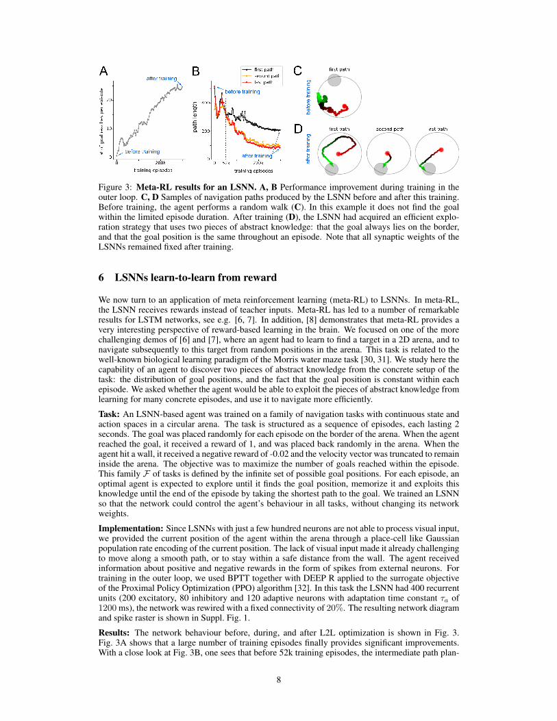
Figure 3: Meta-RL results for an LSNN. A, B Performance improvement during training in theouter loop. C, D Samples of navigation paths produced by the LSNN before and after this training.Before training, the agent performs a random walk (C). In this example it does not find the goalwithin the limited episode duration. After training (D), the LSNN had acquired an efficient explo-ration strategy that uses two pieces of abstract knowledge: that the goal always lies on the border,and that the goal position is the same throughout an episode. Note that all synaptic weights of theLSNNs remained fixed after training.

6 LSNNs learn-to-learn from reward

We now turn to an application of meta reinforcement learning (meta-RL) to LSNNs. In meta-RL,the LSNN receives rewards instead of teacher inputs. Meta-RL has led to a number of remarkableresults for LSTM networks, see e.g. [6, 7]. In addition, [8] demonstrates that meta-RL provides avery interesting perspective of reward-based learning in the brain. We focused on one of the morechallenging demos of [6] and [7], where an agent had to learn to find a target in a 2D arena, and tonavigate subsequently to this target from random positions in the arena. This task is related to thewell-known biological learning paradigm of the Morris water maze task [30, 31]. We study here thecapability of an agent to discover two pieces of abstract knowledge from the concrete setup of thetask: the distribution of goal positions, and the fact that the goal position is constant within eachepisode. We asked whether the agent would be able to exploit the pieces of abstract knowledge fromlearning for many concrete episodes, and use it to navigate more efficiently.

Task: An LSNN-based agent was trained on a family of navigation tasks with continuous state andaction spaces in a circular arena. The task is structured as a sequence of episodes, each lasting 2seconds. The goal was placed randomly for each episode on the border of the arena. When the agentreached the goal, it received a reward of 1, and was placed back randomly in the arena. When theagent hit a wall, it received a negative reward of -0.02 and the velocity vector was truncated to remaininside the arena. The objective was to maximize the number of goals reached within the episode.This family F of tasks is defined by the infinite set of possible goal positions. For each episode, anoptimal agent is expected to explore until it finds the goal position, memorize it and exploits thisknowledge until the end of the episode by taking the shortest path to the goal. We trained an LSNNso that the network could control the agent’s behaviour in all tasks, without changing its networkweights.

Implementation: Since LSNNs with just a few hundred neurons are not able to process visual input,we provided the current position of the agent within the arena through a place-cell like Gaussianpopulation rate encoding of the current position. The lack of visual input made it already challengingto move along a smooth path, or to stay within a safe distance from the wall. The agent receivedinformation about positive and negative rewards in the form of spikes from external neurons. Fortraining in the outer loop, we used BPTT together with DEEP R applied to the surrogate objectiveof the Proximal Policy Optimization (PPO) algorithm [32]. In this task the LSNN had 400 recurrentunits (200 excitatory, 80 inhibitory and 120 adaptive neurons with adaptation time constant τa of1200 ms), the network was rewired with a fixed connectivity of 20%. The resulting network diagramand spike raster is shown in Suppl. Fig. 1.

Results: The network behaviour before, during, and after L2L optimization is shown in Fig. 3.Fig. 3A shows that a large number of training episodes finally provides significant improvements.With a close look at Fig. 3B, one sees that before 52k training episodes, the intermediate path plan-

8

ning strategies did not seem to use the discovered goal position to make subsequent paths shorter.Hence the agents had not yet discovered that the goal position does not change during an episode.After training for 300k episodes, one sees from the sample paths in Fig. 3D that both pieces of ab-stract knowledge had been discovered by the agent. The first path in Fig. 3D shows that the agentexploits that the goal is located on the border of the maze. The second and last paths show thatthe agent knows that the position is fixed throughout an episode. Altogether this demo shows thatmeta-RL can be applied to RSNNs, and produces previously not seen capabilities of sparsely fir-ing RSNNs to extract abstract knowledge from experimentation, and to use it in clever ways forcontrolling behaviour.

7 Discussion

We have demonstrated that deep learning provides a useful new tool for the investigation of networksof spiking neurons: It allows us to create architectures and learning algorithms for RSNNs withenhanced computing and learning capabilities. In order to demonstrate this, we adapted BPTTso that it works efficiently for RSNNs, and can be combined with a biologically inspired synapticrewiring method (DEEP R). We have shown in section 4 that this method allows us to create sparselyconnected RSNNs that approach the performance of LSTM networks on common benchmark tasksfor the classification of spatio-temporal patterns (sequential MNIST and TIMIT). This qualitativejump in the computational power of RSNNs was supported by the introduction of adapting neuronsinto the model. Adapting neurons introduce a spread of longer time constants into RSNNs, as theydo in the neocortex according to [33]. We refer to the resulting variation of the RSNN model asLSNNs, because of the resulting longer short-term memory capability. This form of short-termmemory is of particular interest from the perspective of energy efficiency of SNNs, because it storesand transmits stored information through non-firing of neurons: A neuron that holds information inits increased firing threshold tends to fire less often.

We have shown in Fig. 2 that an application of deep learning (BPTT and DEEP R) in the outer loopof L2L provides a new paradigm for learning of nonlinear input/output mappings by a RSNN. Thislearning task was thought to require an implementation of BP in the RSNN. We have shown that itrequires no BP, not even changes of synaptic weights. Furthermore we have shown that this newform of network learning enables RSNNs, after suitable training with similar learning tasks in theouter loop of L2L, to learn a new task from the same class substantially faster. The reason is thatthe prior deep learning has installed abstract knowledge (priors) about common properties of theselearning tasks in the RSNN. To the best of our knowledge, transfer learning capabilities and the useof prior knowledge (see Fig. 2I) have previously not been demonstrated for SNNs. Fig 3 showsthat L2L also embraces the capability of RSNNs to learn from rewards (meta-RL). For example,it enables a RSNN – without any additional outer control or clock – to embody an agent that firstsearches an arena for a goal, and subsequently exploits the learnt knowledge in order to navigatefast from random initial positions to this goal. Here, for the sake of simplicity, we considered onlythe more common case when all synaptic weights are determined by the outer loop of L2L. Butsimilar results arise when only some of the synaptic weights are learnt in the outer loop, while othersynapses employ local synaptic plasticity rules to learn the current task [27].

Altogether we expect that the new methods and ideas that we have introduced will advance our un-derstanding and reverse engineering of RSNNs in the brain. For example, the RSNNs that emergedin Fig. 1-3 all compute and learn with a brain-like sparse firing activity, quite different from a SNNthat operates with rate-codes. In addition, these RSNNs present new functional uses of short-termmemory that go far beyond remembering a preceding input as in [34], and suggest new forms ofactivity-silent memory [35].

Apart from these implications for computational neuroscience, our finding that RSNNs can acquirepowerful computing and learning capabilities with very energy-efficient sparse firing activity pro-vides new application paradigms for spike-based computing hardware through non-firing.

Acknowledgments

This research/project was supported by the HBP Joint Platform, funded from the European Union’sHorizon 2020 Framework Programme for Research and Innovation under the Specific Grant Agree-ment No. 720270 (Human Brain Project SGA1) and under the Specific Grant Agreement No.

9

785907 (Human Brain Project SGA2). We gratefully acknowledge the support of NVIDIA Cor-poration with the donation of the Quadro P6000 GPU used for this research. Research leading tothese results has in parts been carried out on the Human Brain Project PCP Pilot Systems at theJulich Supercomputing Centre, which received co-funding from the European Union (Grant Agree-ment No. 604102). We gratefully acknowledge Sandra Diaz, Alexander Peyser and Wouter Klijnfrom the Simulation Laboratory Neuroscience of the Julich Supercomputing Centre for their sup-port. The computational results presented have been achieved in part using the Vienna ScientificCluster (VSC).

References[1] Matthieu Courbariaux, Itay Hubara, Daniel Soudry, Ran El-Yaniv, and Yoshua Bengio. Binarized neural

networks: Training deep neural networks with weights and activations constrained to+ 1 or-1. arXivpreprint arXiv:1602.02830, 2016.

[2] Steven K. Esser, Paul A. Merolla, John V. Arthur, Andrew S. Cassidy, Rathinakumar Appuswamy,Alexander Andreopoulos, David J. Berg, Jeffrey L. McKinstry, Timothy Melano, Davis R. Barch,Carmelo di Nolfo, Pallab Datta, Arnon Amir, Brian Taba, Myron D. Flickner, and Dharmendra S. Modha.Convolutional networks for fast, energy-efficient neuromorphic computing. Proceedings of the NationalAcademy of Sciences, 113(41):11441–11446, November 2016.

[3] David Kappel, Robert Legenstein, Stefan Habenschuss, Michael Hsieh, and Wolfgang Maass. Reward-based stochastic self-configuration of neural circuits. eNEURO, 2018.

[4] Guillaume Bellec, David Kappel, Wolfgang Maass, and Robert Legenstein. Deep rewiring: Training verysparse deep networks. International Conference on Learning Representations (ICLR), 2018.

[5] Uri Hasson, Janice Chen, and Christopher J Honey. Hierarchical process memory: memory as an integralcomponent of information processing. Trends in cognitive sciences, 19(6):304–313, 2015.

[6] Jane X Wang, Zeb Kurth-Nelson, Dhruva Tirumala, Hubert Soyer, Joel Z Leibo, Remi Munos, CharlesBlundell, Dharshan Kumaran, and Matt Botvinick. Learning to reinforcement learn. arXiv preprintarXiv:1611.05763, 2016.

[7] Yan Duan, John Schulman, Xi Chen, Peter L Bartlett, Ilya Sutskever, and Pieter Abbeel. RL2: Fastreinforcement learning via slow reinforcement learning. arXiv preprint arXiv:1611.02779, 2016.

[8] Jane X Wang, Zeb Kurth-Nelson, Dharshan Kumaran, Dhruva Tirumala, Hubert Soyer, Joel Z Leibo,Demis Hassabis, and Matthew Botvinick. Prefrontal cortex as a meta-reinforcement learning system.Nature Neuroscience, 2018.

[9] Johannes Schemmel, Daniel Bruderle, Andreas Grubl, Matthias Hock, Karlheinz Meier, and SebastianMillner. A wafer-scale neuromorphic hardware system for large-scale neural modeling. In Circuits andsystems (ISCAS), proceedings of 2010 IEEE international symposium on, pages 1947–1950. IEEE, 2010.

[10] Steve B Furber, David R Lester, Luis A Plana, Jim D Garside, Eustace Painkras, Steve Temple, andAndrew D Brown. Overview of the spinnaker system architecture. IEEE Transactions on Computers,62(12):2454–2467, 2013.

[11] Ning Qiao, Hesham Mostafa, Federico Corradi, Marc Osswald, Fabio Stefanini, Dora Sumislawska, andGiacomo Indiveri. A reconfigurable on-line learning spiking neuromorphic processor comprising 256neurons and 128k synapses. Frontiers in neuroscience, 9:141, 2015.

[12] Mike Davies, Narayan Srinivasa, Tsung-Han Lin, Gautham Chinya, Yongqiang Cao, Sri Harsha Cho-day, Georgios Dimou, Prasad Joshi, Nabil Imam, Shweta Jain, et al. Loihi: A neuromorphic manycoreprocessor with on-chip learning. IEEE Micro, 38(1):82–99, 2018.

[13] Chris Eliasmith. How to build a brain: A neural architecture for biological cognition. Oxford UniversityPress, 2013.

[14] Brian DePasquale, Mark M Churchland, and LF Abbott. Using firing-rate dynamics to train recurrentnetworks of spiking model neurons. arXiv preprint arXiv:1601.07620, 2016.

[15] Dongsung Huh and Terrence J Sejnowski. Gradient descent for spiking neural networks. arXiv preprintarXiv:1706.04698, 2017.

[16] Wilten Nicola and Claudia Clopath. Supervised learning in spiking neural networks with force training.Nature communications, 8(1):2208, 2017.

10

[17] Guillaume Bellec, Darjan Salaj, Anand Subramoney, Robert Legenstein, and Wolfgang Maass. Compu-tational properties of networks of spiking neurons with adapting neurons; in preparation. 2018.

[18] Wulfram Gerstner, Werner M. Kistler, Richard Naud, and Liam Paninski. Neuronal dynamics: Fromsingle neurons to networks and models of cognition. Cambridge University Press, 2014.

[19] Christian Pozzorini, Skander Mensi, Olivier Hagens, Richard Naud, Christof Koch, and Wulfram Ger-stner. Automated high-throughput characterization of single neurons by means of simplified spikingmodels. PLoS computational biology, 11(6):e1004275, 2015.

[20] Nathan W Gouwens, Jim Berg, David Feng, Staci A Sorensen, Hongkui Zeng, Michael J Hawrylycz,Christof Koch, and Anton Arkhipov. Systematic generation of biophysically detailed models for diversecortical neuron types. Nature communications, 9(1), 2018.

[21] Corinne Teeter, Ramakrishnan Iyer, Vilas Menon, Nathan Gouwens, David Feng, Jim Berg, Aaron Szafer,Nicholas Cain, Hongkui Zeng, Michael Hawrylycz, et al. Generalized leaky integrate-and-fire modelsclassify multiple neuron types. Nature communications, 1(1):1–15, 2018.

[22] Tomas Mikolov, Armand Joulin, Sumit Chopra, Michael Mathieu, and Marc’Aurelio Ranzato. Learninglonger memory in recurrent neural networks. arXiv preprint arXiv:1412.7753, 2014.

[23] David Kappel, Stefan Habenschuss, Robert Legenstein, and Wolfgang Maass. Network Plasticity asBayesian Inference. PLOS Computational Biology, 11(11):e1004485, 2015.

[24] Quoc V. Le, Navdeep Jaitly, and Geoffrey E. Hinton. A simple way to initialize recurrent networks ofrectified linear units. CoRR, abs/1504.00941, 2015.

[25] Rui Costa, Ioannis Alexandros Assael, Brendan Shillingford, Nando de Freitas, and Tim Vogels. Corticalmicrocircuits as gated-recurrent neural networks. In Advances in Neural Information Processing Systems,pages 272–283, 2017.

[26] Klaus Greff, Rupesh K Srivastava, Jan Koutnık, Bas R Steunebrink, and Jurgen Schmidhuber. LSTM: Asearch space odyssey. IEEE transactions on neural networks and learning systems, 2017.

[27] Anand Subramoney, Guillaume Bellec, Franz Scherr, Robert Legenstein, and Wolfgang Maass. Recurrentnetworks of spiking neurons learn to learn; in preparation. 2018.

[28] Matthew G Perich, Juan A Gallego, and Lee E Miller. A neural population mechanism for rapid learning.Neuron, 2018.

[29] Sepp Hochreiter, A Steven Younger, and Peter R Conwell. Learning to learn using gradient descent. InInternational Conference on Artificial Neural Networks, pages 87–94. Springer, 2001.

[30] Richard Morris. Developments of a water-maze procedure for studying spatial learning in the rat. Journalof neuroscience methods, 11(1):47–60, 1984.

[31] Eleni Vasilaki, Nicolas Fremaux, Robert Urbanczik, Walter Senn, and Wulfram Gerstner. Spike-basedreinforcement learning in continuous state and action space: when policy gradient methods fail. PLoScomputational biology, 5(12):e1000586, 2009.

[32] John Schulman, Filip Wolski, Prafulla Dhariwal, Alec Radford, and Oleg Klimov. Proximal policy opti-mization algorithms. arXiv preprint arXiv:1707.06347, 2017.

[33] Allen Institute. c© 2018 Allen Institute for Brain Science. Allen Cell Types Database, cell feature search.Available from: celltypes.brain-map.org/data. 2018.

[34] Gianluigi Mongillo, Omri Barak, and Misha Tsodyks. Synaptic theory of working memory. Science (NewYork, N.Y.), 319(5869):1543–1546, March 2008.

[35] Mark G. Stokes. ‘Activity-silent’ working memory in prefrontal cortex: a dynamic coding framework.Trends in Cognitive Sciences, 19(7):394–405, 2015.

11