long-range persistence in climatological and hydrological time series

Journal

&dogy

Journal of Hydrology 203 (1997) 198-208

Long-range persistence in climatological and hydrological time series: analysis, modeling and application to drought hazard assessment

Jon D. Pelletier”, Donald L. Turcotte

Department of Geological Sciences. Snee Hall Cornell University, Ithacu, NY 14853. USA

Received 22 January 1997; revised 15 May 1997; accepted 25 August 1997

Abstract

We present power spectra of time-series data for tree ring width chronologies, atmospheric temperatures, river discharges and precipitation averaged over hundreds of stations worldwide. The average power spectrum S for each of these phenomena is found to have a power-law dependence on frequency with exponent -l/2: S(f) xf-‘/‘. An advection-diffusion model of the vertical transport of heat and water vapor in the atmosphere is presented as a first-order model of climatic and hydrological variability. The model generates variability with the observed spectrum. The model is validated with a correlation anaiysis of temperature and water vapor concentration measurements from the TIROS operational vertical sounder (TO%). Drought frequency analyses based on synthetic lognormal streamflows with the above power spectrum are presented. We show that the presence of long memory as implied by the power-law power spectrum has a significant effect on the likelihood of extended droughts compared with the drought hazard implied from standard autoregressive models with short memory. 0 1997 Elsevier Science B.V.

Keywords: Time-series analysis; Fractals; Diffusion; Drought

1. Introduction

It is generally recognized that there is persistence in climatological and hydrological time series over a wide range of time scales. Persistence for a temperature time series means that warm years (or days or weeks) are, more often than not, followed by warm years and cold years by cold years. The same cluster- ing is recognized in other time series such as precipitation and river discharge. Hurst (1951) and Hurst et al. (1965) presented studies of these correlations using the resealed-range technique. They found that a variety of climatological and hydrological time series produced a power-law resealed-range plot

* Corresponding author.

0022-1694/97/$17.00 0 1997 Elsevier Science B.V. All rights reserved PI1 SOO22- 1694(97)00 102-9

with an average exponent of 0.73. No persistence would yield an exponent of 0.5. One interpretation of the power-law resealed range plot is that persistence is self-similar with variability on long time scales larger than on short time scales. In a series of papers, Mandelbrot and Wallis (1968, 1969a, b, c, d) introduced a class of models called fractional gaussian noises that yield a power-law resealed-range plot. Fractional gaussian noises have autocorrelation functions with a power-law dependence on time lag (Beran, 1994). This contrasts with autoregressive models which have autocorrelation functions that are exponential as a function of time lag.

In this paper we present the results of new analyses intended to address the nature of persistence in climatological and hydrological time series. In particular,

J.D. Pelletier. D.L. Turcotte/Joumal of Hydrology 203 (1997) 198-208 199

we present evidence that the average power spectrum It has been argued that even if the Hurst phenom- of different climatological and hydrological processes enon is valid and time series have long-range persis- is S(f) Kf -‘12. The power spe ctrum is defined as the tence, this is of doubtful practical value is reservoir square of the coefficients in a Fourier series represen- storage applications (Klemes et al., 1981). One appli- tation of the time series. It shows the variance of the cation in which long-range persistence is crucial is function at different frequencies. We show that the drought hazard assessment. Since hydrologic drought shape of the average power spectrum of different climatological and hydrological processes (S(f) m f -‘12)

is a phenomenon which depends on low river discharge over an extended period of time, assessing

is consistent with the results of Hurst et al. (1965). We the nature of serial correlations in a river flow is essen- chose the power spectrum as the method of analysis tial to determining the likelihood of severe drought. because it is superior to other methods such as the To show this we have compared the drought fre- resealed-range method. In a comparison study of the quency of synthetic lognormal time series based on resealed-range, autocorrelation, relative dispersion, an AR(l) model and fractional noise (fn) with and power spectrum techniques of fractional gaussian S(f) m’ 1/2 for the Colorado river. The drought fre- noises, Schepers et al. (1992) concluded that spectral quencies predicted by the fn model differ substantially analysis yielded the least biased results and the lowest from those of an AR( 1) process, with the discrepancy variance in its estimates of the fractal dimension. increasing with drought duration. For instance, a Autocorrelation and resealed-range analysis, on the drought of 10 years duration for the Colorado has a other hand, yielded biased results under many circum- recurrence interval of 100 years according to the fn stances. In our analysis we computed the power model and a recurrence interval of 500 years accord- spectra of many time series for a given quantity and ing to the AR(l) model. We present the results of then averaged the spectra at equal frequency values to drought frequency analyses on synthetic streamflows identify the average power spectral behavior of the with the observed spectrum S(f) x f “* that gives the process. The results of precipitation records, however, recurrence interval as a function of the duration, mag- indicate persistence only at time scales greater than 10 nitude of the drought and the parameters of the log- years. normal distribution.

Perhaps the strongest criticism for power-law power spectral behavior in climatological and hydrological variations has been the lack of a physical mechanism for it (Klemes, 1974). However, since the pioneering work of Whittle (1962) on agricultural variability it has been known that some stochastic partial differential equations yield solutions with long-range persistence in space and time. In this paper we show that a model of the turbulent transport of heat and water vapor in the atmosphere gives rise to a gaussian or lognormal time series with power spectrum S(f) x f -“2, consistent with the results of our power spectral analysis. The model makes the assumption that vertical transport can be modeled by constant velocity advection superimposed on diffusion with a constant eddy diffusivity in the troposphere. This parametrization of the atmospheric turbulent transport is validated by a correlation analysis of TIROS operational vertical sounder measurements. This model suggests that power-law autocorrelations are a possible model for climatological and hydrological variability.

2. Power spectra of climatological and hydrological time series

In Fig. 1 we present the average normalized power spectrum of monthly mean temperature from 94 stations worldwide on a logarithmic scale. The power spectra were computed with the routine “spctrm” of Press et al. (1992) using a Bartlett window. This routine uses the technique of Welch (1967) which divides each record up into four subsets, estimates the power spectrum of each subset, and then averages the estimates at equal frequency values. This procedure provides a better estimate of the power spectrum, but does not provide an estimate of the power at the lowest four frequencies. The power at those frequencies was estimated using the “spctrm” routine without dividing the data into subsets. We computed the power spectra of all complete temperature series of length greater than or equal to 1024 months from the climatological database complied

200 J.D. Pellefier. D.L. Turcotte/Journal qf Hydrology 203 (1997) 198-208

I l$_’

h 1 10-21

-iJYL- i_i _.-i-l 10-2 10-l loo 10'

f (l/wr)

Fig. 1. Averaged normalized power spectrum of 94 monthly temperature time series (with the annual variability removed) as a function of frequency.

by Vose et al. (1992). The annual variability was removed by subtracting from each monthly data point the average temperature for that month in the total record for each station. The power spectra of each record estimated as described above were then averaged at equal frequencies. The slope indicated in the graph is the result of a least-square fit to the logarithms (base 10) of the power spectrum and frequency. The data yield an average power spectrum with a slope of -0.43.

Fig. 2 illustrates the results of a similar analysis performed on the monthly mean river discharge data

,o_,r -- -__, -11, 1 __I_~_~._ ~

“\i ‘-\\i

slope=-0.50 1

\\

-L-d_.,- _ 1 . 2.-__.~J .:I

10-2 10-l loo 10' f (l/year)

Fig. 2. Averaged normalized power spectrum of 636 monthly river discharge series (with the annual variability removed) as a function of fequency.

10-l

1o-3 10-2 10-l

f (l/year)

Fig. 3. Averaged normalized power spectrum of 43 tree ring chronologies in the western US as a function of frequency.

from the Hydro-Climatic Data Network compiled by Slack and Landwehr (1992). The power spectrum was computed in the same manner as for the temperature data. For the streamflow data we chose all complete records with a duration greater than or equal to 5 12 months, including 636 records in the analysis. A least- square fit to the logarithms of the power spectra yield a slope of -0.50, similar to the slope observed in the temperature data. We have taken advantage of the large number of available stations to investigate the possible regional variability of the power spectra. We have averaged the power spectra for each of the 18 hydrologic regions of the US defined as in Wallis et al. (1991). All of the regions exhibited the same spectral dependence with an average exponent of -0.52 and a standard deviation of 0.03, indicating little variation.

We have also performed an analysis of tree ring width chronologies in the western United States obtained from the International Tree Ring Data Bank (National Geophysical Data Center, 1997). Tree rings in the western US are often strongly corre- lated with precipitation. The chronologies are time series in which the nonstationarities in growth rates have been removed and spatial averaging has been performed in an attempt to isolate climatic effects. Tree ring series have the advantage of being much longer than most historical records. We obtained 43 chronologies in the western US with greater than 1024 years of length. The average normalized power spectra of those records are presented in Fig. 3. The

J.D. Pelletier, D.L. Turcotte/Joumal of Hydrology 203 (1997) 198-208 201

slope of the least squares fit indicates that for tree ring time series, Sy> is nearly proportional tof-‘12.

Vattay and Hamos (1994) have performed spectral analysis on humidity time series from time scales of a day to several decades. They identified a power-law power spectrum with exponent -0.61, consistent with our results for temperature, river discharge and tree ring chronologies.

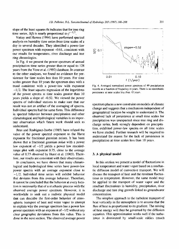
In Fig. 4 we present the power spectrum of annual precipitation time series greater than or equal to 128 years from the Vose et al. (1992) database. In contrast to the other analyses, we found no evidence for persistence for time scales less than 10 years. For time scales greater than 10 years the spectrum rises with a trend consistent with a power-law with exponent - l/2. The least squares regression of the logarithms of the power spectra at time scales greater than 10 years yields a slope of -0.52. We viewed the power spectra of individual stations to make sure that our result was not an artifact of the averaging of spectra. Individual spectra had the same form. This difference in spectral behavior between precipitation and other climatological and hydrological variables is an impor- tant observation which future work should seek to understand.

Bras and Rodriguez-Iturbe (1985) have related the value of the power spectral exponent to the Hurst exponent for fractional gaussian noises. It has been shown that a fractional gaussian noise with a power law exponent of -l/2 yields a power law rescaled- range plot with exponent 0.75, close to the average value of 0.73 observed by Hurst et al. (1965). There- fore, our results are consistent with their observations.

In conclusion, we have shown that many climatological and hydrological time series have power-law power spectra with an average exponent close to -l/2. Individual time series will exhibit behavior that deviates from this average behavior. Therefore, it cannot be concluded that the behavior at every location is necessarily that of a stochastic process with the observed average power spectrum. However, it is worthwhile to seek out a realistic physical model that can describe the first-order behavior of atmospheric transport of heat and water vapor to attempt to explain why the average spectrum has a power law power spectrum with an exponent of -l/2 without any clear geographic deviations from this value. This is done in the next section. The observed average power

I , LldA __--___~-.L~ _-.i

0.01 0.10 f (l/wr)

Fig. 4. Averaged normalized power spectrum of 49 precipitation records as a function of frequency in years. There is no identifiable persistence at time scales less than IO years.

spectrum places a new constraint on models of climate change and suggests that a mechanism independent of geographical location be sought to understand it. The observed lack of persistence at small time scales for precipitation was unexpected since tree ring and discharge series, both strongly dependent on precipitation, exhibited power-law spectra on all time scales we have studied. Further research will be required to understand the reason for the lack of persistence in precipitation at time scales less than 10 years.

3. A physical model

In this section we present a model of fluctuations in local temperature and water vapor based on a stochastic diffusion model of convective transport. We will discuss the transport of heat and the resultant fluctuations in temperature. However, the same model may be applied to the transport of water vapor and the resultant fluctuations in humidity, precipitation, river discharge and tree ring growth linked to groundwater concentration.

The simplest approach to the turbulent transport of heat vertically in the atmosphere is to assume that the flux of heat is proportional to its gradient. The mixing of heat energy will then be governed by the diffusion equation. This approximation works well if the turbulence is dominated by small-scale eddies (much

smaller than that of the mean gradient of potential temperature) where the convective action of turbulent eddies is analogous to the molecular collisions responsible for molecular diffusion (Moffatt, 1983). This assumptiobn is an accurate one for a neutral or stably stratified troposphere, but breaks down for a highly convective one (Garratt, 1992). Diffusive transport has been assumed in analytical models of climate change in the atmosphere (North, 1975; Ghil, 1983) and in the ocean where diffusion com- bined with global advection is a well-established zero-order model (Munk, 1966). Experimental and theoretical observations support the hypothesis that diffusive transfer accurately models vertical transport in the atmosphere. Kida (I 983) has traced the dispersion of air parcels in a hemispheric GCM and found the transport to be diffusive in the troposphere. Hofmann and Rosen (1987) have argued that vertical turbulent diffusion is the best model of the exponential decay of aerosol from the El Chichon volcanic eruption. Vertical atmospheric turbulent diffusion is superimposed, as it is in oceanic diffusion, on large- scale Hadley and Walker circulations (Peixoto and Oort, 1992).

In order to test the hypothesis that diffusion superimposed on large-scale circulation is a realistic first- order model of atmospheric transport, we have performed a correlation analysis of temperature and water vapor concentration vertically in the atmosphere measured with the TIROS operational vertical sounder (TOVS). The analysis of temperature data was presented in Pelletier (1997). Here we present the results for water vapor concentration. The results are nearly identical to that of temperature data. We obtained 2 months (January-February 1985) of daily TOVS data of gridded precipitable water vapor with 1” horizontal spatial resolution at pressure levels of 1000, 850, 700, 500 and 300 mbar.

The time series of precipitable water vapor concentration was detrended with a least-squares linear fit to remove the annual trend and leave only the high- frequency variations. For a fixed horizontal location and a fixed time lag, the detrended water vapor concentration at one elevation, h,, was multiplied by the detrended water vapor concentration at another elevation, hi. These products were averaged for all pairs of data separated by the same distance r = kz, - hZl normalized by the product of the standard deviations

\~ 0.6

‘\ T;‘

‘_

u 0.4 t=2 _ .

t=3 ‘!

o.2 y& . .

o.. t=6

0 2 4 6 8

r (km)

0.6 ‘\_ \_

‘\

‘\

j\

t=3 \

0.2 it=4 ,t=5

0.0 Jr 6__~-. __.- 0 2 4 6 8

r (km)

Fig. 5. Spatial cross-correlation functions of (a) TOVS measure-

ments of precipitable water vapor and (b) those for an advection-

diffusion model of vertical atmospheric transport with N = 0.01 m s-’ and D = 100 m’s_’ for t = 1. 2, 3, 4, 5 and 6 days

with the correlation decreasing with increasing time lag

of both time series to obtain the spatial cross- correlation function. The cross-correlation function for a one-dimensional diffusion process is given by the solution to a one-dimensional diffusion process with constant velocity advection characterized by a velocity u and diffusivity D (Voss and Clarke, 1976):

(1)

The spatial cross-correlation as a function of vertical distance for time lags t = 1, 2, 3, 4, 5 and 6 days are presented in Fig. 5(a). The functions given by Eq. (1) for u = 0.0 1 m s-’ and D = 100 m” s-’ 1 are presented

J.D. Pelletier, D. L. Turcotte/Joumal qf Hydrology 203 ( 1997) 198-208 203

in Fig. 5(b). The advection-diffusion correlation functions of Fig. 5(b) bear resemblance to the spatial cross-correlations of the TOVS data. The advection term is consistent with large-scale advection by Hadley and Walker circulations. Superimposed on the transient eddies that we model as diffusive there is a steady-state vertical advection of heat and water vapor by Hadley and Walker circulations. The globally averaged velocity of local vertical advection is 0.003 m SC’ (Peixoto and Oort, 1992), close to the observed globally averaged velocity, 0.01 m s-‘, from the TOVS analysis presented in Fig. 5. The diffusivitiy of D = 100 m* SC’, estimated with a least-squares linear fit of ln(c(r,l)) vs Y*, is roughly consistent with, but somewhat larger than, the tradi- tional estimate of 10 m2 SC’ (Peixoto and Oort, 1992). We conclude from this analysis that an advection- diffusion model is a reasonable first-order model of large-scale atmospheric transport of heat and water vapor. In our modeling we will focus only on the effect of diffusive transport on the local fluctuations of heat and water vapor. The advective transport would lead to only a periodicity in the time series of local temperature or water vapor with an average period of about 2 weeks (the return time for tropo- spheric circulation with u = 0.01 m s-l). No such periodicity was identified in the time series presented in Section 2.

In addition to the diffusive nature of turbulent mixing in the atmosphere, it is also necessary to model the random advection of heat and moisture vertically in the atmosphere by convective instabilities. To incorporate this stochastic component, we will add a noise term to the flux of a deterministic diffusion equation for heat and water vapor vertically in the atmosphere. Such a random term is consistent with atmospheric dynamics implied from variations on the length of the day. From time scales of 1 month to several years, variations in the length of the day are caused by the vertical transport of moisture in the atmosphere modulating the earth’s moment of inertia (Rosen et al., 1990). The power spectrum of variations in the length of the day over this range of time scales is S(f) x f’ (Eubanks et al., 1985), consistent with a random, uncorrelated advection of water vapor mass vertically in the atmosphere. In this section, we investigate the fluctuations in local temperature expected from a stochastic diffusion model of turbulent heat

transport and compare our predictions with instru- mental records.

To see how time series with power-law power spectra arise, we present the results from the simu- lation of a discrete, one-dimensional stochastic diffusion process. A discrete version of the diffusion equation for the density of particles on a one- dimensional grid of points is

We establish a one-dimensional lattice of 32 sites with a periodic boundary conditions at the ends of the lattice. At the beginning, we place 10 particles on each site of the lattice. At each timestep, a particle is chosen at random and moved to the left with probability l/2 and to the right if it does not move to the left. In this way, the average rate at which particles leave a site is proportional to the number of particles in the site. The average rate at which particles enter is proportional to the number of particles on each side multiplied by one half (since the particles to the left and right of site i move into site i only half of the time). This is a stochastic model satisfying Eq. (2). The probabilistic nature of this model causes fluctuations to occur in the local density of random walkers that do not occur in a deterministic model of diffusion.

In Fig. 6 we present the average of 50 power spectra of the time series of the number of particles in the

Fig. 6. Average normalized power spectrum of the number of

random walkers in the central site of a lattice. The average of 50

simulations is presented.

204 J.D. Pellerirr. D.1.. 7;rrcottr/Journtrl oI’ H\‘t/ro/o,c~ X.3 ( IYY 7) I OX--LOX

0.0 t 0.0 0.2 0.4 0.6 0.8

normolized mognitude m

Fig. 7. Cumulative distribution function of the time series produced by the stochastic diffusion model (solid circles). The solid line represents the cumulative lognormal distribution function fit to the data.

central site of the 32-site lattice. The figure shows a power spectrum of the form Scf) “f-‘I*.

In Fig. 7 we plot the cumulative probability distribution of the time series produced by the stochastic diffusion model. The solid circles represent data. The line represents the cumulative lognormal distribution fit to the data. A good fit is obtained.

Since the distribution of values in a hydrological time series is often lognormal, we have shown that a simple model of turbulent transport gives rise to both the power spectrum and the distribution observed for hydrological time series.

A stochastic diffusion process can be studied analytically by adding a noise term to the flux of a deterministic diffusion equation (Van Kampen, 1981):

8AT aJ War=-%

J= -c~g+q(x,t)

(3)

where AT are the fluctuations in temperature from equilibrium and r(x,r) is gaussian, white noise.

We will calculate the power spectrum of temperature fluctuations in a layer of width 21 exchanging heat with an infinite, one-dimensional, homogeneous space as in Fig. 8. The presentation we give is nearly the same as that of Voss and Clarke (1976).

The Fourier transform of the heat flux of the

4 4 4

21 I : E(t)

4 4

Fig. 8. Geometry of the one-dimensional diffusion calculation detailed in the text.

stochastic diffusion equation is

iwrl(k, w) J(kw)= Dk’

The rate of change of heat energy in the layer will be given by the difference in heat flux out of the bound- aries, located at ?z I:

dE(f) -=J(1,t)-J(-1,r) dt

The Fourier transform of E(t) is then

E(w) = -L J x

(27r)‘GJ ---1 sin(kl)J(k, w) dk (6)

The power spectrum of variations in E(f), SE(a) = < IE(w)l’ > is

J x

SE(W) sin’(U)

e-7. D2k4+w' dk x w-'/' (7)

for low frequencies. Since AT x AE, S&w) x w-‘/’ also. We obtain the same results as with the discrete model.

Pelletier (1997) has presented further studies of stochastic diffusion as a model for the natural variability of climate. He presented the power spectrum of fluctuations in a stochastic diffusion model in a two- layer geometry with thermal and diffusion properties appropriate to the atmosphere and the ocean with a radiative boundary condition at the top of the atmospheric layer. We found a broad region proportional to ,f -112 up to time scales of 2000 years. At lower frequencies the results we obtained were consistent with the power spectrum of the Yostok Deuterium ice core, a proxy for local atmospheric temperature.

4. Application to drought hazard assessment

If long-range persistence exists in nature, there is perhaps no area of hydrology more affected than that

J.D. Pelletier, D.L. Turcotte/Journal of H.ydrology 203 (1997) 198-208 205

of drought hazard assessment. This has been recognized by Bras and Rodriguez-Iturbe (1985) who begin their discussion of long-range persistence in the context of droughts. They remark that ARIMA models aften underestimate the frequency of historic drought. Attempts to “fix” short memory models by including dependences at longer lags do not remove this problem because if the time scale is lengthened, more unexpectedly large droughts will occur (Bras and Rodriguez-Iturbe. 1985). This is a motivation for long-memory models such as fractional noises.

Since hydrologic droughts are a phenomena requir- ing multiple years of low flow, the frequency of occur- rence will be affected by correlations in the time series of discharge. In this section, we illustrate how fractional noises can be used to estimate drought frequencies. The use of fractional noises that exhibit the Hurst phenomenon has been advocated by Booy and Lye (1989) for use in flood frequency analysis. The goal of stochastic hydrology is to generate synthetic time series of river discharge that most accurately reproduce hydrological time series. Based on our evidence that time series with a power-law power spectrum with exponent -l/2 are universal, we generated synthetic time series with that power spectrum and a two-parameter lognormal distribution that fit the historical record of a river’s discharge. We first discuss the techniques and results of drought frequency analyses for series with different lognormal distribu- tions. Then we show the results of a comparison between drought frequencies for the Colorado river based upon a fractional noise with exponent of -112 and a short-memory AR( 1) model.

We have generated fractional noises with the Fourier-filtering technique. This technique proceeds in several steps: (1) a gaussian white noise sequence is generated; (2) the Fast Fourier transform of the data is computed; (3) the complex Fourier coefficients are multiplied by a factor fp12 (where 0 is the power spectral exponent of the noise desired); (4) the inverse power spectrum is taken; and (5) the moments are resealed. The values can be transformed with the exponential function if a lognormal distribution is desired. The details of the technique are discussed in Turcotte (1992).

There is no unique definition of a drought. Several possibilities are discussed in a recent drought

assessment of the southwestern US by Tarboton (1994). Perhaps the most straightforward definition is that proposed by Yevjevish (1967) and Dracup et al. (1980). They defined a drought as any year or consecutive number of years during which average annual streamflow is continuously below the long- term mean annual runoff. The magnitude is the average deficit during the drought. The principal drawback to this definition is that two 5-year droughts separated by 1 wet year will only be recognized as give year droughts even though the succession of droughts results in 10 or 11 years of critically low supply. Nevertheless, we will accept this as our working definition of a drought.

In Fig. 9(a)-(c) we present the results of drought frequency analyses based on this definition of a drought. Each figure is a two-dimensional contour plot of the logarithm (base 10) of the recurrence interval of a drought of a given duration and magnitude. The magnitude has been normalized by the mean how. To construct each figure we generated synthetic records of one million years in length and searched them for drought occurences. Fig. 9(a), (b) and (c) represent coefficients of variation 0.2, 0.4 and 0.6, respectively. As expected, droughts are least probable for flows with a small coefficient of variation. The recurrence intervals increase nearly exponentially as a function of drought duration, as indicated by the nearly equal spacing of logarithmic contour intervals as the duration of the drought increases. These figures provide a quick reference for estimating the recurrence time of droughts of any magnitude and duration for rivers which have coefficients of variation close to these values. The recurrence intervals for droughts in rivers which have a coefficient of variation different from those assumed in Fig. 9(a)-(c) can still be estimated with a weighted geometric average of the recurrence intervals for the coefficients of variation used for the figure. We propose that these graphs may be useful for estimating drought hazard in regions of the world where hazard assessments based on tree ring chronologies are prohibitively expensive.

In order to assess the importance of long-range persistence on the likelihood of severe drought, we have completed a drought frequency analysis on a fractional noise model for the Colorado river at Lees Ferry and a published AR( 1) model constructed from

0 5 10 15 20 durotion (years)

0.00 ~I _-_..

0 5 10 15 20 duration (yeors)

0.50 F

4 0.40 f- ,

.e h 0 0.30 E

x .N 0.20 L E E b c 0.10:

0.00 L 0 5 10 15 20

duration (years)

Fig. 9. Logarithm (base IO) of the recurrence interval as a function of drought duration and magnitude (normalized by the mean annual flow) for a lognormal distribution with coefficient of variation (a) 0.2, (b) 0.4, and (c) 0.6.

1 i / I 0.00 L >_i

0 5 10 15 20 duration (years)

0.00 _ _’ ____’ ~_ ‘_- ‘~_ ’ .~ //I I i/j

0 5 10 15 20 duration (yews)

Fig. 10. Logarithm (base IO) of the recurrence interval as a func-

tion of drought duration and magnitude (normalized by the mean annual flow) for (a) a fractional lognormal noise model of the

Colorado River at Lees Ferry with fl = l/2 and a coefficient of

variation of 0.27, and (b) the AR(I) model for the Colorado River at Lees Ferry developed by Kendall and Dracup ( 1991).

the same location by Kendall and Dracup (1991). Contour plots of the logarithm (base 10) of the recurrence intervals are plotted in Fig. 10(a) and (b) for the fractional noise and AR(l) model, respectively. The coefficient of variation for the lognormal fractional noise model was computed to be 0.27 from the historic time series in Kendall and Dracup (1991). The fractional noise synthetic streamflow was constructed with the same coefficient of variation of 0.27 and the observed power spectrum S(f) x.f‘ - ‘/2. There are significant difference between the two contour maps. For instance, for droughts of 10 years duration and small magnitude, the recurrence interval

J.D. Pelletier, D.L. Turcotte/Joumal of Hydrology 203 (1997) 198-208 201

according to the fn model is 100 years while the recurrence interval for the AR(l) model is 500 years. We conclude that the presence of long-range persistence has a significant effect on the likelihood of severe drought. The presence of long-range persistence does not, however, appear to increase the ability to predict future climatological and hydrological time series to any significant degree (Noakes et al., 1988).

5. Conclusions

We have presented the results of power spectral analyses that make a compelling case for long-term persistence in climatological and hydrological time series. We have presented a model for long-term persistence based on a stochastic diffusion model of the flucutations in heat and water vapor transport in the atmosphere that predicts the observed spectrum. Diffusive transport of heat and water vapor vertically in the atmosphere was verified with a correlation analysis of TOVS measurements. Lastly, we have argued that long-range persistence can have a dramatic effect on the likelihood of severe hydrologic drought and we have computed recurrence intervals for droughts of different magnitudes, durations and coefficients of variation.

Acknowledgements

We wish to thank Jim McWilliams for suggesting the analysis of the TOVS data. The TOVS data were produced through funding from the Earth Observing System Pathfinder Program of NASA’s Mission to Planet Earth in cooperation with National Oceanic and Atmospheric Administration. The data were pro- vided by the Earth Observing System Data and Infor- mation System (EOSDIS), Distributed Active Archive Center at Goddard Space Flight Center which archives, manages and distributes this data set.

References

Beran, J., 1994. Statistics for Long-Memory Processes, Chapman and Hall, New York.

Booy, C., Lye, L.M., 1989. A new look at flood risk determination, Water Resour. Bull., 25, 933-943.

Bras, R.L., Rodriguez-Iturbe, I.. 1985. Random Functions in

Hydrology. Addison-Wesley, Reading, MA. Dracup, J.A., Lee, K.S., Paulson. E.G., 1980. On the statistical

characteristics of drought events, Water Resour. Res., 16, 289-296.

Eubanks, T.M., Steppe, J.A., Dickey, J.O.. Callahan, P.S., 1985. A spectral analysis of the earth’s angular momentum budget. J. Geophys. Res., 90, 538555404.

Garratt, J.R., 1992. The Atmospheric Boundary Layer. Cambridge University Press, New York.

Ghil, M., 1983. Theoretical climate dynamics: An introduction. In: M. Ghil (Ed.), Turbulence and Predicability in Geophysical Fluid Dynamics and Climate Dynamics. North Holland, Amsterdam.

Hofmann, A.J., Rosen, J.M., 1987. On the prolonged lifetime of the El Chichon sulfuric acid aerosol cloud. J. Geophys. Res., 92, 982.5-9830.

Hurst, H.E., 195 I. Long-term storage capacity of reservoirs, Trans. Am. Sot. Civ. Engng, 116, 770-808.

Hurst, H.E., Black, R.P., Simaika, Y.M., 1965. Long-term Storage: An Experimental Study. Constable, London.

Kendall. D.R., Dracup, J.A., 1991. A comparison of index-sequen- tial and AR(l) generated hydrologic sequences, J. Hydrol., 122, 335-352.

Kida, H., 1983. General circulation of air parcels and transport characteristics derived from a hemispheric GCM part 2: Very long-term motions of air parcels in the troposphere and stratosphere, J. Meteor. Sot. Jap.. 51. 510-522.

Klemes, V.. 1974. The Hurst phenomenon: a puzzle’?. Water Resour. Res.. IO, 675-688.

Klemes, V., Srikanthan, R., McMahon, T.A.. 1981. Long-memory flow models in reservoir analysis: what is their practical value‘?. Water Resour. Res.. 17, 137-75 I.

Mandelbrot, B.B., Wallis. J.R., 1968. Noah, Joseph, and operational hydrology, Water Resour. Res., 4. 909-9 18.

Mandelbrot, B.B., Wallis, J.R., 1969. Computer experiments with fractional Gaussian noises. Part I. averages and variances, Water Resour. Res., 5, 228-24 I.

Mandelbrot, B.B., Wallis, J.R., 1969. Computer experiments with fractional Gaussian noises. Part 2. resealed ranges and spectra. Water Resour. Res., 5. 242-259.

Mandelbrot, B.B., Wallis, J.R., 1969. Computer experiments with fractional Gaussian noises. Part 3. mathematical appendix, Water Resour. Res., 5. 260-267.

Mandelbrot, B.B., Wallis, J.R.. 1969. Some long-run properties of geophysical records. Water Resour. Res., 5. 32 I-340.

Moffatt, H.K., 1983. Transport effects associated with turbulence. Rep. Prog. Phys.. 46, 625-664.

Munk. W.H.. 1966. Abyssal recipes. Deep-Sea Res., Ii. 707-730. National Geophysical Data Center. International Tree Ring Data

Bank, electronic data, available from http://www.ngdc.noaa. gov/paleo/treering.html or Mr. Bruce Bauer, National Geo- physical Data Center, 325 Broadway EGC, Boulder, CO 80303.

Noakes, D.J., Hipel. K.W., McLeod. A.I.. Himenez, C.. Yakowitz. S.. 1988. Forecasting annual geophysical time series. Int. J. Forecasting, 4. IO3- I 15.

208 J. Il. Pellrtier, D. L. Turc,otte/Jounlctl of Hwfmlo<~~ 203 ( 19071 19%208

North, G.R.. 1975. Analytical solution to a simple climate model

with diffusive heat transport, J. Atmos. Sci.. 32, 1301-1307. Pelletier, J.D., 1997. Analysis and modeling of the natural varia-

bility of climate, J. Climate. IO. 1331-1342. Peixoto, J.P., Oort. A.H., 1992. Physical of Climate. American

Institute of Physics. New York. Press, W.H., Teukolsky. S.A.. Vetterling. W.T.. Flannery, B.P..

1992. Numerical Recipes in C: The Art of Scientific Com- puting, 2nd edn. Cambridge University Press, New York.

Rosen, R.D.. Salstein, D.A., Wood, T.M., 1990. Discrepancies in the earth-atmosphere angular momentum budget, J. Geophys. Res.. 95, 265-279.

Schepers, H.E., van Beek. J.H.G.M.. Bassingthwaighte, J.B., 1992. Four methods to estimate the fractal dimension from self-affine signals, IEEE Engng Med. Bio., June, 57-64.

Slack, J.R., and Landwehr, J.M., 1992. US Geological Survey Open-File Report 92-129: Hydro-Climatic Data Network: A US Geological Survey Streamflow Data Set for the United States for the Study of Climatic Variations: 1874-1988. US Geological Survey, Reston, VA.

Tarboton, D.G., 1994. The source hydrology of severe sustained drought in the south-western United States, J. Hydrol.. 161,3 I - 69.

Turcotte, D.L., 1992. Fractals and Chaos in Geology and Geo- physics. Cambridge University Press. New York.

van Kampen, N.G.. 1981. Stochastic Proce\\ea tn Physic\ and Chemistry. North-Holland. Amsterdam.

Vattay. G.. Hamos. A.. 1994. Scaling behavtor in daily ari humidity fluctuations. Phys. Rev. Lett.. 73. 768-77 I.

Voae, R.S., Schmoyer. R.L.. Stcwer. P.M.. Peterson. T.C Hcim. R.. Karl, T.R.. Etscheid, J.K.. 1992. The Global Historical Climatology Network: Long-term Monthly Temperaturc, Pre- cipitation, Sea-level Pressure, and Statton Pressure Data. Environmental Sciences Division Pub. No. 392. Oak Ridge National Laboratory. Oak Ridge, TN.

Voss. R.F.. Clarke, J.. 1976. Flicker (I/f) noise: Equilibrium temperature and resistance fluctuations. Phys. Rev. B. Ii. 5566573.

Wallia. J.R.. Lettenmaier. D.P.. Wood, E.F., 1991. A daily hydro- climatological data set for the continental US. Water Resour. Res.. 27. 1657-1663.

Welch. P.D., 1967. The use of the Fast Fourter Transform for the estimation of the power spectrum: a method based on averaging over short, modified periodograms. IEEE Trdns. Audio Electroacoust.. IS. 70-73.

Whittle. P.. 1962. Topographic correlation, power-law covariance functions, and diffusion, Biometrika, 49, 304-314.

Yevjevish. V.M., An objective approach to definitions and investigations of continental hydrologic droughts. 1967. Hydrol. pap. 23. Cola. State Univ., Fort Collins. CO.

long-range persistence in climatological and hydrological time series

Documents