PSYCHOMETR1KA--VOL. 61, NO. 3, 401-425SEPTEMBER 1996

LOGIT MODELS AND LOGISTIC REGRESSIONS FOR SOCIAL NETWORKS:I. AN INTRODUCTION TO MARKOV GRAPHS AND p*

STANLEY WASSERMAN

UNIVERSITY OF ILLINOIS

PHILIPPA PATTISON

UNIVERSITY OF MELBOURNE

Spanning nearly sixty years of research, statistical network analysis has passed through (atleast) two generations of researchers and models. Beginning in the late 1930’s, the first generationof research dealt with the distribution of various network statistics, under a variety of null models.The second generation, beginning in the 1970’s and continuing into the 1980’s, concerned models,usually for probabilities of relational ties among very small subsets of actors, in which’ varioussimple substantive tendencies were parameterized. Much of this research, most of which utilizedlog linear models, first appeared in applied statistics publications.

But recent developments in social network analysis promise to bring us into a third generation. TheMarkov random graphs of Frank and Strauss (1986) and especially the estimation strategy for thesemodels developed by Strauss and Ikeda (1990; described in brief in Strauss, 1992), are very recentand promising contributions to this field. Here we describe a large class of models that can be usedto investigate structure in social networks. These models include several generalizations of sto-chastic blockmodels, as well as models parameterizing global tendencies towards clustering andcentralization, and individual differences in such tendencies. Approximate model fits are obtainedusing Strauss and Ikeda’s (1990) estimation strategy.

In this paper we describe and extend these models and demonstrate how they can be used toaddress a variety of substantive questions about structure in social networks.

Key words: categorical data analysis, social network analysis, random graphs.

1. Introduction The Evolution of Statistical Models for Social Networks

Statistical models have been used by researchers to study social networks for almost60 years, beginning with the work of the early sociometricians in the late 1930’s. The goalof these models was (and remains) the quantitative examination of the stochastic proper-ties of social relations and the actors of a particular network. Nonstochastic models havecertainly been considered by many, but such models do not have the nice properties oftheir statistical counterparts, such as goodness-of-fit statistics and the possibility of para-metric significance tests of various network structural properties.

Recent developments in social network analysis have now brought us to a new gen-eration of models, namely the Markov random graphs of Frank and Strauss (1986) andespecially the estimation strategy for these models developed by Strauss and Ikeda (1990),described in brief in Strauss (1992). These models expand considerably the class of struc-

This research was supported by grants from the Australian Research Council and the National ScienceFoundation (#SBR93-10184). This paper was presented at the 1994 Annual Meeting of the Psychometric Society,Champaign, Illinois, June 1994. Special thanks go to Sarah Ardu for programming assistance, Laura Koehly andGarry Robins for help with this research, and to Shizuhiko Nishisato and three reviewers for their comments.INTERNET email addresses: pattison@psych.unirnelb.edu.au (PP); stanwass@uiuc.edu (SW). Atfiliations: De-partment of Psychology, University of Melbourne (PP); Department of Psychology, Department of Statistics, andThe Beckman Institute for Advanced Science and Technology, University of Illinois (SW).

Requests for reprints should be sent to Stanley Wasserman, University of Illinois, 603 East Daniel Street,Champaign, IL 61820.

0033-3123/96/0900-95265500.75/0© 1996 The Psychometric Society

401

402 PSYCHOMETRIKA

tural models that can be investigated within the exponential family first proposed byHolland and Leinhardt (1981). Markov models, and their more general forms, which labelp*, can be approximated by logistic regressions, thus giving the researcher easy accessto a very large wealth of modeling tools.

The review and extension of this research is the goal of this and our companion paper(Pattison & Wasserman 1995).

We first give some notation which we will use throughout, and then turn to a briefrecent history of statistical models for social networks. More thorough historical accountscan be found in chapters 13-16 of Wasserman and Faust (1994).

2. Some Notation

A social network is defined as a set of 9 social actors and a collection of r socialrelations that specify how these actors are relationally tied together. Of interest to us herewill be networks with either r = 1 or 2 relations. Examples of social relations are "choosesas a friend" and "is a neighbor of", recorded for each pair of individuals in some set ofactors.

We let ~ denote a set of actors: ~/" = {1, 2 .... ,9}. A dichotomous social relation, ~g,is a set of ordered pairs recording relational ties between pairs of actors. If the ordered pair(i, j) is in this set, then the first actor (i) in the pair has a relational tie to the second actor(j) in the pair; we write iXj, or more succinctly, i --~ j.

A social relation can be either directed (i’s tie to j may differ from j’s tie to i) nondirected (there is, at most, one nondirected tie connecting i and j), and can also valued (the tie from i to j has a nondichotomous strength or value). The main statisticalfocus in the literature has been on models for single (or univariate), dichotomous, directedrelations (represented as directed graphs). Since many of the models described here take ona different character when the relation under study is nondirected, we will (at times)describe the models and parameters which arise when the relation is not directed.

Any social relation can be represented by a 9 × g sociomatrix, X, where the (i, j) entryin the matrix (which we denote by X(i, j) or, sometimes, by Xij) is the value of the tie fromactor i to actorj on that relation. For a dichotomous relation, X is also the adjacency matrixof the directed graph representing the relation. For a valued relation, X(i, j) = c, the value "of the tie fromi toj. We typically assume that c ~ {0, 1, 2,..., C - 1}. For adichotomous relation, C = 2, so that

{~ ifi--’,jX(i, j) otherwise.

Frequently of interest in network analysis are subsets of actors and all the ties that mightexist among them. For example, for a dichotomous relation, a dyad is a pair of actors andall the ties between them, and can be in one of four states: null (no ties), asymmetric (onetie; two possibilities), and mutual (two ties).

In the general, multirelational case, relational ties are recorded for r relations. Weassume that these relations, ~1, ~2, ̄ ¯ ¯, ~/~r, have associated sociomatrices Xl, X2,..., Xr.And since these sociomatrices will be assumed to be random quantities, we will uselower-case bold-face characters (such as x) to denote realizations of these random quan-tities. Our focus here is on the univariate situation (r = 1), while extensions to themultivariate situation can be found in the companion paper (Pattison & Wasserman,1995).

Important network statistics for dichotomous directed relations include the outdegreeand indegree of an actor, that is, the number of ties sent and received (Xj X(i, j) and~i X(i, j), respectively); the number of ties, L = ~i,j X(i, j), and the number of recipro-

STANLEY WASSERMAN AND PHILIPPA PAq’TISON 403

cated ties (that is, such that X(i, j) = X(j, i) = 1; sometimes referred to as mutual dyads);and numbers of higher-level subgraphs, such as 2-out-stars (triples of nodes such thati --~ j and i --~ k), 2-in-stars (triples of nodes such that j ~ i and k ~ i), 2-mixed-stars(triples of nodes such that i ~ j and k -~ i), cyclic triads (triples such that i ~ j, j ~ k -~ i), and so on (there are many possibilities). We define

M = ~ X(i, j)X(j, i<j

as the number of mutual dyads,

as the number of 2-out-stars,

T=

S = ~ X(i,j)X(i, i.~j~k

~ X(i,j)X(j, k)X(k, i~j~k

as the number of cyclic triads, all for a single relation.A (directed) path of length d from i to j is a sequence of nodes {i = i 1, i 2 .....

id+1 = j}, beginning with i and ending with j, such that

X(il, i2)X(i2, i3) ... X(id, id + 1) = 1.

The shortest path between any pair of nodes is a geodesic, and the length of the geodesic(s)is the distance from i to./(denoted by dij). This geodesic distance can be defined a bit moreformally as

dij = minimum value of k for which

X(io, il)X(il, i2) ¯ ¯ ¯ X(ik_ 1, ik) =

where i 0 = i and i k = j. The distance dij is undefined if there is no path from i toj. A graphis "disconnected" if some distances are undefined; the graph is then said to have more thanone component. In a digraph, if at least one node has no path to another node, the digraphis not strongly connected.

If actors have been partitioned into a set of S blocks (or positions), we can define ~ij;rsas an indicator variable, equal to 1 if actor i is in the rth block and actor j is in the sth.

There are many other simple graph statistics; some of these will be presented in latersections (see Tables 1 and 2 for nondirected relations and Tables 3 and 4 for directedrelations).

We will let O and ~r be symbols to represent logits--log odds ratios, comparing theprobability of one outcome of a random variable to the probability of another outcome, ina logarithm scale. The O’s will be logits based on Holland and Leinhardt’s (1981) models,while the ~r’s will be logits based on the p* models that we describe here.

3. A Brief History

The models that are considered in this paper express each relational tie as a stochasticfunction of actor or network structural properties. An important example of such a modelis Holland and Leinhardt’s (1977, 1981)Pl model. The pl model includes parameters fortie density, the propensity for reciprocity of ties, and individuals’ tendencies to express andreceive tie~. This model and its many generalizations make the strong assumption of dyadicindependence, an assumption that has been criticized in the literature (see chapter 15 ofWasserman & Faust, 1994). Consequently, developments which relax the assumption are

404 PSYCHOMETRIKA

of considerable importance. Frank and Strauss’ (1986) research on Markov random graphswas the first such generalization, and has great potential. Markov graphs permit depen-dencies among any ties that share a node (for example, Xij and Xi~, or Xij and Xj~).

The important work of Strauss and Ikeda (1990) has made these models computa-tionally available. Strauss and Ikeda investigated apseudolikelihood estimation procedure,a generalization of maximum likelihood, that uses an approximate likelihood functionwhich does not assume dyadic independence (see comments in Iacobucci & Wasserman1990; and chapters 15 and 16 of Wasserman & Faust 1994). Strauss and Ikeda derived pseudolikelihood/~s a function of each data point (xij), conditional on the rest of the data.Any interdependencies in the data can be directly modeled by this statistical conditioning,so no assumptions need to be made that the data points are all independent.

Strauss and Ikeda compared the performance of standard maximum likelihood (ML)estimates to their maximum pseudo-likelihood (MP) estimates both in a simulation study,and by analyzing the "like" relation measured on the monks in the monastery studied bySampson (1968). In the simulations, they looked at the performance of the estimates in fivereplicated networks containing fifteen, twenty, or thirty actors. They found that MP andML estimates performed equally well, as evaluated by a root mean squared error measure.The estimates had greater standard errors for the networks with fewer actors, but thiswould be true of any procedure--better precision usually occurs with larger data sets.

Under all the conditions for which both ML and MP estimates could be estimated, thetwo performed similarly. One of the main advantages in the use of MP estimation is thatthere are conditions under which MP estimates exist, but ML estimates do not. In addition,the MP approach further expands the applicability of pl because it can be used to fitmodels that do not assume dyadic independence, such as those described by Frank andStrauss (1986).

Strauss and Ikeda’s comparisons also address the issue of how well the maximumlikelihood estimation ofpl parameters performs even under conditions where the assump-tion of dyadic independence is known to be violated. The fact that the ML estimates areas good as MP estimates is good news. One can proceed to use the relatively simplemethods without much concern that violation of the assumption of dyadic independencewill greatly affect the results. The biggest advantage (to us) of the MP estimation techniqueis its ease of use--as we note below, logistic regression computational procedures can beused to fit these models, and hence, to give very good approximations of fitted pl-typemodels.

Details of such models, which we will refer to here by p*, follow.

4. Pl, P*, and Logit Models

Before describing the models, p 1 and p*, we note that we will illustrate the methodsdescribed here on an example taken from Vickers and Chan (1981) and Vickers (1981).They obtained network data from 29 students in Grade 7 in a school in Melbourne,Victoria in Australia. They asked the students to nominate their classmates on a numberof relations, including the following:

Who do you get on with in the class?¯ Who are your best friends in the class?¯ Who would you rather not be friends with?¯ Who would you prefer to work with? and¯ Who would you rather not work with?

Each of these questions gives rise to a dichotomous relation, with measurements recordedin a 29 × 29 sociomatrix. We focus our attention here on the first relation ("Getting on

STANLEY WASSERMAN AND PHILIPPA PATrlSON 405

with"), and the fourth ("Work with"). Both of these relations are directed. We label two, ~g, and ~w (for Get on With, and Work with). The two matrices for these relationsare shown in Tables 11 and 12 found in the Appendix.

We note that Actors 1 through 12 are boys, while Actors 13 through 29 are girls. Wewill use these data to illustrate the models described below.

4.1. Pl

We quickly reviewpl, referring the reader to more complete treatments (Fienberg Wasserman, 1981; Holland & Leinhardt, 1981; Reitz, 1982; Wasserman, 1987; Wasserman& Faust, 1994; Wasserman & Galaskiewicz, 1984) if needed.

Consider the dyad Dij = (Xij, X~i), and the four possible states that this randomquantity can be in:

¯ (Sij , Xji ) = (0, 0)--Null dyad,¯ (Xij, X~i) = (1, 0)--Asymmetric dyad (i --~j),¯ (Xij, Xji) = (0, 1)--Asymmetric dyad (j --~ ¯ (gij , Sji ) = (1, 1)--Mutual dyad.

We consider the substantive tendencies which might cause a particular dyad to be in oneof these states (for example, mutual dyads might arise if both actors were quite popular).Such tendencies are then incorporated as additive effects into a model for the logarithmsof the probabilities of the four dyadic states.

We first create a new matrix, Y, from X, which aids the computations for the model.We define the entries of this g × /7 × 2 × 2 matrix as follows:

Yij~a --- { ~ ifotherwise.the dyad D ij takes on the values (Xi~ = k, X~i = l) (1)

Thus, the four entries in Y which are associated with the pair of actors i and j (the 2 × submatrix associated with the ith level of variable 1 and thejth level of variable 2) code thestate of the dyad Dij. To specify pl, we postulate the following log linear equations:

log P(Y000 = 1)

log e(YijlO = 1) = hij +

log e(Yijol = 1) = hi~ + 0

log P(Y/i11 = 1) Aij + 20+ Ol i "[-

"~- O~i -~ ~j

+ ~j + f~i

c~ + ~ + f~ + p. (2)The parameters of this model are explained at length in Fienberg and Wasserman (1981),Wasserman (1987), or chapter 15 of Wasserman and Faust (1994). In brief, the a’s reflectsubstantive tendencies toward expansiveness (they are "subject" effects), the/3’s, attrac-tiveness or popularity ("partner" effects), 0 is an overall choice parameter, while p modelstendencies toward reciprocation or mutuality.

If the relation in question is not directed, then model (2) has a simpler form. Fornondirected relations, there are only two dyad states, and only two types of parameters(see Wasserman & Faust, 1994).

Perhaps a better way to present this model is to relax the restriction to dichotomousrelations. We can assume that the relation is valued, and that every tie has a strength, witha score measured on.an integer scale from 0 to C - 1. If we define k as the value of thetie from i toj and l as the value of the tie fromj to i, then we can generalize Y so that itselements Yijkl = 1, when Xi] = k and Xyi = l. The following model statement (from

406 PSYCHOMETRIKA

Wasserman & Iac0bucci, 1986; see also Anderson & Wasserman, 1995) generalizes thefour statements of p 1:

log P(Y/jkt = 1) = A,.j Ok+ Ot + Oli (k) ~- Olj(l) "~- ~j(k) ~- ~i(l ) q- Dkl" (3)

Regardless of the nature of the relation, dyads are assumed to be statistically inde-pendent, so that the joint probabilit~ distribution, and hence the likelihood function, issimply a product of dyadic probabilities. Models such as Pl are referred to as dyadicindependence models (for obvious reasons).

Estimation (after placing necessary and logical constraints on model parameters),fitting, and testing are described in any of the above references. Simplifications arise ifrelations are ordinal, or if actors can be assumed to fall naturally into subgroups (so thatactor-level parameters can be equated for all actors within a particular subgroup). Fittingis not particularly easy, and the asymptotic theory for testing is questionable (at best).These two problems (along with the desire for models that do allow dyads to be depen-dent) motivate the research into more complicated models that we now present. Thesemodels have the useful feature that they include dyadic independence models such as Plas a special case.

4.2. p*--Theory, Special Cases, Estimation

In order to specify the exponential family of models p*, which contains Markovrandom graphs, as well asp1 as a special case (in a sense that we mention below), we needa bit more notation. From X, the sociomatrix for a single, dichotomous, directed relation,we define three new relations, with sociomatrices easily constructed from X. First, wedefine Xi~- as the sociomatrix for the relation formed from 9g where the tie from i to j isforced to be present: Xi~? = {Xkl , with Xij = 1}. Next, we define Xi7 as the sociomatrix forthe relation formed from 2( where the tie from i toj is forced to be absent (or to be at level0): Xi7 = {Xkt, with Xiy = 0}. Lastly, we define X~ as the complement relation for the tiefrom i to j: X~ = {Xkt, with (k, l) :/: (i,j)}. The complement relation has no relational coded from i to j--one can view this single variable as missing. All told, these three newrelations are needed to define p*.

The original specification of these models was just for a single, dichotomous relation.Most of the early work focused on nondirected relations. Generalizations to valued rela-tions, and to more than one relation, were mentioned in passing (in concluding remarks)by Frank and Strauss (1986, see. 6) and by Strauss and Ikeda (1990, sec. 5). We address of these generalizations in this paper and in our companion paper, Pattison and Wasser-man (1995).

4.2.1. Logit Models

We now describe the general, log linear form of p*, which we will then present in itslogit formulation. We begin with log linear models of the form

exp {0’z(x)}Pr (X = x) = K(0) (4)

where 0 is a vector of model parameters and z(x) is a vector of network statistics. Thesemodels are of exponential family form, in which the probability function depends on anexponential function of a linear combination of network statistics. Such models arisefrequently, not only for studies of social networks, but also in spatial modeling, statisticalmechanics, and even in test theory (Strauss, 1992). We refer to models of the form (4)

STANLEY WASSERMAN AND PHILIPPA PATTISON 407

the label p*. One might need constraints on the elements of 0 to insure a set of uniquely-determined parameters (as we illustrate later with our examples).

In model (4) for social networks, the 0 parameters are the weights of the linearcombination, and are usually unknown, and hence, must be estimated. The function ~, inthe denominator of model (4), is a constant that insures that the probability distribution indeed proper, summing to one over the sample space of the random variable X--allpossible directed graphs. Examples of variou.s statistics z are numerous, and (for a directedrelation) include the number of mutual dyads, M, the number of ties, L, and the outdegreeof the ith actor, xi+. A very wide range of such statistics can be found in Tables 1, 2, 3,and 4.

A very simple example of model (4), which is quite similar to the simplest Bernoulligraph distribution as well as to a special case of pl, is

exp { OL }Pr(X=x)= ~(0) (5)

with a single parameter 0 and which depends on only the number of relational ties.The problem with distributions of this form is the normalizing constant. In order for

probabilities to be computed, one must be able to calculate ~, which is just too ditiicult formost networks. This prevents easy maximum likelihood estimation of the model parame-ters (see Frank & Strauss, 1986) except in special circumstances. But, there are tricks, Fienberg and Wasserman (1981) discovered for P l, and as we describe below, for p*.

As described by Strauss and Ikeda (1990), one can turn this loglinear model into logit model, using the dichotomous nature of the random variable Xij. We first conditionon the complement of Xij, and consider just the probability that the tie from i to j ispresent:

Pr (X = xi~-)Pr (Xij = lIx~) = Pr (X = xi~+) + Pr (X = xi~-)

exp {O’z(xi~- )}

= exp {0’z(xi; )} + exp {O’z(x/f)} (6)

which has the advantage of not depending on the normalizing constant. We next considerthe odds ratio of the presence of a tie from i toj to its absence, which simplifies model (6):

Pr (Xij IlX 0) exp ’ +_~. c {0 Z(Xlj )}

Pr (Xij : 0lX~j) exp {0’z(x~i )}

= exp {0’[z(xi7 ) - z(xif )]}. (7)

From this, the log odds ratio, or logit, model has the rather simple expression:

Pr l[X~j)~ = Ot[z(xi;) z(xi)-)].(8)

<Xijwiy = log ~rr (Xij 01x )J

If we define ~(xij ) = [z(xi~-) - z(xi])], then the logit model (8) simplifies succinctly wij= O’~(xij). The expression ,5(xij ) is the vector of network statistics that arises when thevariable Xij changes from 1 to 0. This version of the model, in which a log odds ratio isequated to a linear function of the components of B(xij), will be referred to as the logit p*model for a single, dichotomous relation.

As one can see, to specify a logit p* model, one chooses a priori a collection ofnetwork statistics that is supposed to affect the log odds of a tie being present to absent.

408 PSYCHOMETRIKA

The model itself depends on the hypothesized structural features of the network. For eachhypothesized structural feature (such as transitivity), there is a corresponding networkstatistic (such as, T, the total number of transitive triads) and a corresponding "explanatoryvariable" in the logit model; the explanatory variable is the change in the network statisticwhen the tie from node i to node j changes from being present to absent.

The model is easy to construct when the relation is dichotomous, so that logits aresimple and well-defined. When the relation is valued, one must be careful about whichlogits to model--there will be C - 1 logits fo[ a dichotomous relation that takes on integervalues from 0 to C - 1. We discuss this at length in Pattison and Wasserman (1995).

4.2.2. Dependence Graphs

In the original specification of model p*, Frank and Strauss (1986) viewed it as generalization of model Pl and all its relatives, designed to relax the restriction of theearlier models to independent dyads. Frank and Strauss first presented p* as a modelincorporating a complicated dependence structure for nondirected relations, and thengeneralized this to directed relations. Even though Frank and Strauss (1986) presented thegeneral specification of p*, they concentrated (as can be seen by the title of that paper) the special case ofp* incorporating a Markov assumption. This special case is based on thetheory for Markov random fields, applied to graphs (and hence, labeled Markov randomgraphs). As Frank and Strauss desired, one no longer had to assume that dyads werestatistically independent.

Markov graphs are generalizations of Markov random fields designed for spatialinteraction models (Kindermann & Snell, 1980; Ripley, 1981; Speed, 1978; Strauss, 1977),and are based on the work of Ising (1925) for models of rectangular arrays .of binaryvariables, or lattices (Wasserman, 1978). Any two sites on a lattice are neighbors if they aresufficiently close. One then postulates an Ising model for the entire set of lattice variableswhich has the same exponential family form as model (4) with parameters

There are a variety of ways of viewing p*. One important aspect or view of thesemodels is the dependence structure they assume for the lines of the graph or arcs of thedigraph. A dependence graph, in the context of a social network, indicates which relationalties (or subsets of relational ties) are conditionally independent. The dependence structureof a random directed graph is simply a graph whose nodes are all possible relational tiesin the original relation and whose ties specify which ties in the relation are conditionallydependent, given the remaining relational ties. Two ties are conditionally dependent if theconditional probability that the ties both are present, given the other ties in the network,is not equal to the product of their marginal conditional probabilities. The dependencegraph has lines connecting all pairs of conditionally dependent ties. There are many waysof specifying conditional dependence between a pair of ties, which lead to a variety ofdistinct dependence graphs.

For example, the dependence digraph arising from Pl has lines connecting eachrelational tie to its dyadic pair (and no others). Other examples are described below.

To fully appreciate this view of p*, one needs to consider the structure of the depen-dence graph and how a particular structure is reflected inp* model parameters. We do thisformally, using the Hammersley-Clifford theorem (discussed by Besag, 1974) which estab-lishes that a random directed graph has a probability that depends only on the completesubgraphs of the dependence graph. (A complete subgraph of a graph is a subset of nodesin which every pair of nodes in the subset is linked by a line. Thus, a complete subgraphin the dependence graph corresponds to a set of ties in the original random directed graph,every pair of which is conditionally dependent, given the rest of the graph.) The theoremalso establishes that sufficient statistics for a loglinear model for the random directed graph

STANLEY WASSERMAN AND PHILIPPA PATTISON 409

are of the form II (i,j)~A Sij, whereA is a complete subgraph of the dependence graph. Theproduct here is computed across a set of edges in the original directed graph that arepairwise mutually conditionally dependent. The induced subgraph in the original directedgraph corresponding to this set of edges is termed a sufficient subgraph for the loglinearmodel. (The subgraph induced byA is simply the collection of all edges inA and the nodesin the original graph to which they are incident.) This important result implies that oneneed only worry about complete subgraphs of the dependence graph.

Frank and Strauss described several important examples of specific dependence struc-tures.

1. The first" is the case of a Bernoulli directed graph, in which all edges are condition-ally independent. The dependence graph of a Bernoulli graph comprises a collectionof isolated nodes, each corresponding to an edge in the Bernoulli graph.

2. A second is the case of dyad independence in which Xij is conditionally dependentonly on ~t~i, given the rest of the graph (Strauss & Ikeda, 1990). In this case, thecomplete subgraphs of the dependence graph are of the form {Xij} or {Xij, X~.i}.

3. A third type of dependence structure is one in which edges that have an actor incommon are conditionally dependent (Frank & Strauss, 1986). From this, Frank andStrauss define a Markov directed graph as a random directed graph for which arcs inthe dependence graph connect pairs of possible ties if and only if they have an actorin common, such as Xij and Xik , Xij and Xki , Xij and Xjk, or Xij and Xkj. It imme-diately follows that in a Markov graph, the complete subgraphs of the dependencegraph are simply triads and k-stars. In a Markov digraph, the complete subgraphs ofthe dependence graph are mutual dyads, triads, and stars of order 3 or more. Frankand Strauss give the complete subgraphs (with 4 or fewer nodes) of the dependencegraph of a Markov digraph.

Frank and Strauss’ use of Markov (di)graphs greatly simplifies the possible depen-dence structures that can arise, and leads naturally to a class of parametric models. Spe-cifically, loglinear models for graphs with Markov dependence can be seen to depend onlyon the complete set of triads and k-stars, and not on tetrads or other more complicatedsubgraphs (we note that such subgraph structures are defined in chapter 4 of Wasserman& Faust, 1994). Further simplifications of such models arise with assumptions of homo-geneity of model parameters, and assumptions that some parameters are zero.

Occasionally, it may make sense to propose more complex dependence structures.Suppose, for instance, that there is a coloring on the nodes of a graph or directed graph(that is, each node in the graph is assigned exactly one color from a specified set of colors).The coloring may specify the status of network actors on some attribute such as familymembership; in this case, the coloring would require as many colors as there are families(and we assume, in this simple example, that each actor is a member of exactly one family).We define a block random graph to be a p* random graph in which two possible ties (i, j)and (k, l) are conditionally dependent if and only if nodes i, j, k and l all have the samecolor; in other words, ties are conditionally dependent if they are incident to nodes of thesame color. The corresponding dependence graph consists of a set of disconnected com-ponents, one for each color in the color set and each component is complete. The completesubgraphs of the dependence graph are thus the collection of these components and all oftheir subgraphs. Suiiicient statistics for the corresponding log linear model parameters areproducts of observed ties, where the products are taken over subsets of ties linking indi-viduals of the same color. A block random graph would allow one to model interdepen-dencies among relational ties among family members.

410 PSYCHOMETRIKA

4.2.3. Some Models

To generate a specific member of the logitp* family, one needs to spedfy the vector ofnetwork statistics z(x) and to determine the need for any constraints on the parameters

As shown by Frank and Strauss (1986), one Markov graph model for a nondirectedrelation depends on the number of cyclic triads and the numbers of k-stars in the graphrepresentation of the relation. Such a model needs k-stars as high as k = (9 - 1), and low as k = 1 (the number of ties), so there are exactly (/7 - 1) + 1 = g components z(x). One need not work with a more complicated model, assuming of course, that onewants homogeneity (parameters not depending on the individual actors).

A simpler Markov graph model used by Frank and Strauss (1986) is referred to as thetriad model and depends only on the number of relational ties, L, the number of 2-stars,S, and the number of cyclic triads, T. A special case of this model is one-dimensional, anddepends only on S, the number of 2-stars, and is referred to as the clustering model. Thislatter model is the only model that Frank and Strauss estimate with maximum likelihood.For a directed relation, the model becomes more complicated, since there are differenttypes of stars (for example, there are "in-stars" of order 2, for which both ties end at actori, as well as "out-stars" of order 2, for which both ties originate at actor i; and of course,there are many different types of triad counts).

Another special Markov directed graph model mentioned by Strauss and Ikeda(1990), is the model:

{Pr(Xq = 1IX;.)/z~ij = log ~r (Xij 0lxij--~j = 0 + p(xji) + ai +/3j. (9)

This special case ofp* is similar top1, and so we label itp~. There is also a version of thismodel for nondirected relations, similar to nondirectedpl (see chapter 15 of Wasserman& Faust, 1994), and one can easily add blockmodel-type parameters, as do Wasserman andGalaskiewicz (1984) and Wang and Wong (1987) to Pl. Nondirected p~ is equivalent nondirectedp 1, since the relational ties are actually completely independent (in this specialinstance).

We can put model (9) into the standardp* model form. First define the vector 0 the (2g + 2)-dimensional parameter vector with components

0 = (0, O~1 .... , ag, ~1, " ¯ ¯ , ~g,

where one would constrain the (x’s and the 13’s in some way (perhaps both sets of parameters would sum to zero). With this choice of 0, the vector of graph statistics is

z(x) (L,x~ + .. .. ,x g+ , x + l .. .. ,x+g, M)’,

so that the vector of changes in z(x) that arises when xij changes from a 1 to a 0 is

~(xq) = (1, 0,..., 0, 1, 0 ..... 0, 0,..., 0, 1, 0,..., 0, x~i)’,

where the l’s fall in the first, (i + 1)st, and (g + 1 + j)th entries (corresponding to 0, ai, and/3j components of 0).

Thus, it appears thatpl arises as a logitp* model. The components of z(x) forp~ arethe set of indegrees, the set of outdegrees, M, and L, which are also the sufficient statisticsfor the parameters ofp~; however, and most importantly, this special case p] does notassume dyadic independence (as we discuss at bit more at length, later in this section). Oneway to view p ~ is as an alternative method for estimation of the parameters of p 1.

One can takep~ and generalize it in ways not possible with the dyadic independencemodel pl. Such models incorporate graph statistics into z(x) that depend on higher-order

STANLEY WASSERMAN AND PHILIPPA PATTISON 411

graph properties; specifically, counts of the frequencies of the sufficient subgraphs. Addingcounts of k-stars is one possibility--Frank and Strauss’ triad model is an example. Thereare many other possibilities, which we discuss in brief below. One can postulate rathercomplicated "explanatory graph statistics" as components of z(x).

4.2.4. Structural Parameters for Networks

The class of logit models for directed graphs just described allows very considerablebreadth in the formulation of candidate models for a particular relation. As a result, it isimportant to begin to describe what considerations might influence the choice of a modeland to explicate some possible relationships among models. In this section, we reviewbriefly some major themes of structural analysis for networks, and show how such themesmight be reflected in certain types of loglinear models. Our account is not intended to becomprehensive but rather to illustrate how a wide range of questions about networkstructure can be formulated and explored within this framework.

Structural themes. Wasserman and Faust (1994) review descriptive structural analy-ses of single network relations that have been prominent in the network literature. Theseanalyses have dealt with at least three broad themes:

1. The degree of clustering of nodes in a network as well as the presence of cohesivesubsets;

2. Patterns of connectivity and reachability in the network, and especially the distri-bution of centrality and prestige across the actors; and

3. The similarity among network positions and the degree to which network structurecan be summarized in a blockmodel.

In several of these themes, it has been argued that questions about network structureshould be assessed only after allowing for a variety of constraints that may be regarded aslower-level features of the data.

In an early paper, for instance, Holland and Leinhardt (1973, 1979) observed thatrestrictions on the outdegree of each node imposed constraints on possible structuralpatterns that could be observed at a more global level. Similarly, Holland and Leinhardt(1975), Wasserman (1987), and Snijders (1991) have argued that multirelational questionsand questions dealing with triads and other higher-order structures are best assessed onlyafter taking account of the distribution of various nodal or dyadic network properties.Thus, we will consider models that asse~s the degree to which a network is clustered, orcentralized, in the presence of certain lower-level properties of the network.

A basic distinction applying to the parameters of logit models for structural featuresof a network is that between homogeneous and nonhomogeneous effects. An effect isdefined to be homogeneous if it is assumed to be equal for all pairs of nodes i and j; forinstance, the reciprocity effect in thep ] model is assumed to be homogeneous, whereas theexpansiveness and attractiveness effects are not. (Note that Frank and Strauss define model to be homogeneous if all isomorphic graphs have the same probability. Thus, amodel is homogeneous in the sense of Frank and Strauss if all of its parameters arehomogeneous in the sense defined here.)

Nonhomogeneous effects can be further distinguished according to whether they areassumed to vary freely for all pairs of nodes (i, j) or to be subject to equality constraintswithin classes of the set of possible edges of the network. For instance, a stochasticblockmodel (first defined by Fienberg & Wasserman 1981; and elaborated upon by Was-serman & Galaskiewicz 1984; and Wang & Wong 1987) specifies that density effects fornode pairs (i, j) and (k, l) are equal whenever nodes i and k are in the same class, and

412 PSYCHOMETRIKA

Table 1: Homogeneous parameters and graph statistics for logit models fornondirected relations

Label I Parameter Graph statistic z(x)

Homogeneous effectsChoiceClusterability2-stars:

k-stars:

k-paths:

Connectivity

= X++T = Ei,j,k X~jXikX~i

= ~,j,~ X~jX~k

Uk = E~,~,,~,...,~ X~, X~ ... x~

P~ = E~,~,,~,...,~ x~,x~,~ ... x~_,~

N = minimum number of edges whose remov~disconnects the graph (edge connectivity)

Indices of prominence homogeneity (centralization)Ca, = sum of lengths of geodesics (dq)Ca~ = variance of geodesic lengths (dij)

es CE = maximum geodesic length (eccentricity)¢4 Cv = variance of geodesic length sums (d~+)

(closeness centralization)es CD = variance of X~+’s (degree centralization)es C~ = variance of numbers of geodesics

containing i (betweeness centralization)

Association with fixed Y I F

Table 2: Actor-level parameters and graph statistics for logit models fornondirected relations

Label [ Parameter Graph statistic z(x)

Subgroup-specific/Block-level effectsBlock effects [ G, B,, = ~i,~ X06@,

Node-specific/actor-level effectsDifferential choiceDifferential closeness

Differential connectedness

Differential betweeness

X~+ = degree (degree centrality)di. = average geodesic distance

(closeness centrality)N = minimum number of edges incident to i

whose removal disconnects the graphB~ = number of geodesics containing i

STANLEY WASSERMAN AND PHILIPPA PATI?ISON 413

and l are in the same class, of some a priori partitio n of the node set into classes or blocks.More generally, any partition of the set of edges may be used to define equality constraintsfor an effect in a logit model.

Nondirected relations. Tables 1 and 2 set out a collection of possible parameters forlogit models for nondirected network relations. The parameters are distinguished in thetable according to the homogeneity of their associated effects; in addition, they may bedifferentiated by the type of structural property that they are intended to represent and thenature of the conditional dependence among network relations that is presumed to un-derlie them.

For instance, the parameters listed in Tables 1 and 2 reflect structural features suchas: the degree to which a network is dense, and the degree to which denseness variesaccording to some prespecified relation Y or some blockmodel ~; the degree to which thenetwork displays clustering; the degree to which nodes in the network have degree of atleast k, and the degree to which there is variation in nodal degrees; the degree of con-nectivity in the network and the level and variability of connectedness of node pairs; andthe degree to which nodes in the network differ in their connectedness, closeness, andcentrality in the network.

Some of these parameters may be specified in logit models assuming edge indepen-dence (for instance, 0, ~bs, ~rs, and 3’i); some in logit models for Markov random graphs(such as 7, o-, and v~); and some implicitly assume more complex conditional dependencies(such as 7rl~, v, vi, ~bl, ~b2, ~b3, ~b4, ~b6, ~b4(i), and ~b6(i)). For example, the k-path parameter7r/~ allows dependencies among all potential edges lying on paths of length k, in contrastto Markov random graphs which may be conceptualized as permitting dependencies onlyamong edges on paths of length 2.

Note that it is not always easy to specify the pattern of assumed dependencies: theconnectivity parameter v, for instance, is associated with a pattern of dependencies amongedges that might best be regarded as having arbitrary complexity.

The choice of an hypothesized logit model for an observed network relation dependson several considerations, which we now outline.

First, of course, the effects of primary interest (such as clustering, centralization, andso on) are likely to be dictated by theoretical concerns. Indeed, a large number of de-scriptive studies provide some preliminary support to the claim that clustering, central-ization, positional similarity, and so on, are often both theoretically and empirically im-portant network features.

Second, assumptions about conditional dependence among possible edges of thenetwork relation may be recognized by including parameters corresponding to sufficientsubgraphs in a model. Thus, if Markov random graphs are assumed, then models mightcontain parameters for density, clustering and k-stars (for k = 2,...,/7 - 1)~ although,we might also fit models in which some of these parameters are set equal to zero and othersset to be equal to each other across sets of possible edges.

Third, as indicated earlier, it may sometimes be useful to control for lower-ordereffects by including their associated parameters in the logit model. For example, one couldexamine the degree to which a network exhibits clustering after variations among nodes in"expansiveness" have been taken into account. This might be a particularly useful strategywhere the lower-order effects have been constrained by methodological restrictions (forinstance, where the maximum number of nodes mentioned in response to a relationalquestion is limited by design).

Fourth, such effects can be hypothesized to be homogeneous (Table 1) or nonhomo-geneous (Table 2) and, in the latter case, be subject to equality constraints or not. Suchgenerality allows one to focus on a sequence of nested models and a comparison of the fit

414 PSYCHOMETRIKA

of these nested models. It may be noted here that we are allowing any effect of the modelto be subject to equality constraints, not just density, as in stochastic blockmodels (seechapter 16 of Wasserman & Faust, 1994).

For instance, a plausible model for a relation may specify the presence of two sub-groups having denser within-group than between-group ties, and a tendency for a central-ized structure within each group, but the degree of centralization might be hypothesizedto be greater in one group than another. (Thus, in this two-block case, we might proposea logit model that includes four density parameters for within- and between-block rela-tions, and two centralization parameters, one for each subgroup.) Such parameters arelisted in Table 2.

Further, the equality constraints need not be restricted to having the form of ablockmodel; instead, any partition on the set of possible edges may define the equalityconstraints. An example arises in the case where information is available on a secondnetwork relation and where the presence of a relation of this second kind may be regardedas "affecting" the first relation. For instance, for the data presented in Tables 1 through 3,we might propose that the probability of a Work tie between nodes i andj varies accordingto whether i and j are linked by a "Get on With" tie. Such a model has two densityparameters, one for node pairs (i, j) that are linked by a "Get on With" tie, and one fornode pairs not linked in this way. Such parameters are listed at the end of Table 1.

Fifth, we need to consider possible dependencies among effects and insure that thelogit model is identified. Consider, for instance, the nondirected version of the p ~ model,for which the vector z(x) of explanatory statistics consists of the total number of ties L, andthe degree Xi+ of each node i. Since L = Y~ Xi+, there is a linear dependence among theexplanatory variables; hence, we need to impose an additional constraint (such as requiringthat the parameters associated with the degrees sum to zero, ~ ~/i = 0), or that one of theparameters is fixed at zero (~/1 = 0, for example). Some other notable dependencies amongparameters in Table 2 are that block density effects sum to the overall density effect (andthat any differential block effects sum to the overall corresponding effect), that star effectsare dependent on differential choice, overall density, and so forth. Caution is clearlynecessary here.

Directed relations. Some parameters of interest for logit models for directed rela-tions are set out in Table 3 (homogeneous effects and effects subject to equality con-straints) and Table 4 (node-specific effects). As the tables make clear, there are a largenumber of effects of possible interest when modeling a directed graph, including central-ization, clusterability, prestige, connectivity, transitivity, reciprocity, and block effects.Many of the listed node-specific effects are derived from indices of centralization andprestige, reflecting the prominence of these notions in the network literature (see chapter5 of Wasserman & Faust, 1994; see also Faust & Wasserman, 1992; Koehly & Wasserman,1994).

Several of the effects also reflect the frequency of various forms of triads in a directedrelation. For instance, the cyclicity parameter ~’c reflects the frequency of cyclic triads inthe relation. One possible approach, similar in spirit to that described by Holland andLeinhardt (1975, 1978), is to define parameters corresponding to the 16 distinct types triad (the triad isomorphism classes) in a directed relation (see also chapter 14 of Was-serman & Faust, 1994). One can then assess the fit of a number of models of interest,especially the class described by Johnsen (1985, 1986). More complete and complex as-sociation parameters are also possible, such as those focussing on conformity, exchangeand complementarity (see Wasserman, 1987).

STANLEY WASSERMAN AND PHILIPPA PA’Iq’ISON 415

Table 3: Homogeneous parameters and graph statistics for logit models fordirected relations

Label [ Parameter Graph statistic z(x)

Homogeneous effectsChoiceP~eciprocityTransitivityIntransitivityCyclicity2-in-stars2-out-stars2-mixed-stars:

k-in-starsk-out-stars:

3-paths:

k-pathsConnectivity

0

P

TC

0-1

0"2

0"3

:

?3kI

VkO

:

~3

:

1]

M = ~, XiiXiiTr = E~,~.~ X~X~X~T~= E~,~,~ X~X~(1 - X~)Tc = Ei,j,~ XijXjkXki

S1 = ~i,j,k XjiXki

S~ = ~i,~,~ Xi~Xi~S~ = E~,~,~ X~Xi~:

U~t = E~,~,,~,...,~, x~,~X~,~.., x~iUko = ~i,jl,J2,...,J~ Xijl Xij~ ’’’ Xij~

:

:P~ = E~,~x,~,...,~ X,~,X~,~..-X~_~N = minimum number of edges whose removM

disconnects the digraph (edge connectivity)

Indices of prominence homogeneity (centralization/prestige)

¢2¢3

~5

~7

~S

Ca, = sum of lengths of geodesics (dij)Cc~ = variance of geodesic lengths (dij)CE = maximum geodesic length (eccentricity)Cc = variance of geodesic length sums (di+)

(closeness centralization)CD = variance of Xi+’s (degree centralization)CB = variance of numbers of geodesics

containing i (betweeness centralization)Pp = variance of geodesic length sums (d+i)

(proximity group prestige)PD = variance of X+i’s (degree group prestige)

Association with fixed Y I FBlock effects[ (~s

Interpretation of parameters. Parameters corresponding to each of the effects listed inthese tables may be interpreted in terms of their contribution to the "likelihood" ofoccurrence of networks with the relevant feature of interest. For instance, a large positivevalue of a parameter corresponding to an index of clusterability means that clusterablenetworks are more likely to occur (ceteris paribus). Further, this tendency can be assessedstatistically, at least approximately, by comparing the fit of two models, one with theparameter and one without.

Perhaps the most interesting models here are those that begin with the graph statisticsof p], and add counts of k-stars across all actors, or only for those actors in the sameblockmodel class. Latter models with such parameters are referred to as Markov block-

416 PSYCHOMETRIKA

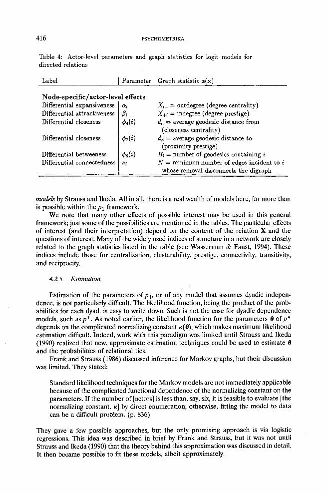
Table 4: Actor-level parameters and graph statistics for logit models fordirected relations

Label ] Parameter Graph statistic z(x)

Node-specific/actor-level effectsDifferential expansivenessDifferential attractivenessDifferential closeness

Differential closeness

Differential betweenessDifferential connectedness

Xi+ = outdegree (degree centrality)X+i = indegree (degree prestige)di. = average geodesic distance from

(closeness centrality)d.i = average geodesic distance to

(proximity prestige)Bi = number of geodesics containing iN = minimum number of edges incident to i

whose removal disconnects the digraph

models by Strauss and Ikeda. All in all, there is a real wealth of models here, far more thanis possible within the Pl framework.

We note that many other effects of possible interest may be used in this generalframework; just some of the possibilities are mentioned in the tables. The particular effectsof interest (and their interpretation) depend on the content of the relation X and thequestions of interest. Many of the widely used indices of structure in a network are closelyrelated to the graph statistics listed in the table (see Wasserman & Faust, 1994). Theseindices include those for centralization, clusterability, prestige, connectivity, transitivity,and reciprocity.

4.25. Estimation

Estimation of the parameters of pl, or of any model that assumes dyadic indepen-dence, is not particularly difficult. The likelihood function, being the product of the prob-abilities for each dyad, is easy to write down. Such is not the case for dyadic dependencemodels, such as p*. As noted earlier, the likelihood function for the parameters 0 of p*depends on the complicated normalizing constant K(0), which makes maximum likelihoodestimation difficult. Indeed, work with this paradigm was limited until Strauss and Ikeda(1990) realized that new, approximate estimation techniques could be used to estimate and the probabilities of relational ties.

Frank and Strauss (1986) discussed inference for Markov graphs, but their discussionwas limited. They stated:

Standard likelihood techniques for the Markov models are not immediately applicablebecause of the complicated functional dependence of the normalizing constant on theparameters. If the number of [actors] is less than, say, six, it is feasible to evaluate [thenormalizing constant, K] by direct enumeration; otherwise, fitting the model to datacan be a difficult problem. (p. 836)

They gave a few possible approaches, but the only promising approach is via logisticregressions. This idea was described in brief by Frank and Strauss, but it was not untilStrauss and Ikeda (1990) that the theory behind this approximation was discussed in detail.It then became possible to fit these models, albeit approximately.

STANLEY WASSERMAN AND PHILIPPA PA’I~ISON 417

The likelihood function for the general form of p*, model (4),

exp {0’z(x)}L(O) - ~(0)

where the dependence on the normalizing constant can easily be seen. An approximateestimation approach, proposed by Strauss (1986) and Strauss and Ikeda (1990), utilizestools made popular in models for rectangular lattices; specifically, we define the pseudo-likelihood function to be

PL(O) = I-I Pr (xi/= l[X~.) x’j Pr (Xij = 01X~)(1 -x,j) (10)

and a maximum pseudolikelihood estimator to be the value of 0 that maximizes (10). estimators are much easier to calculate that ML estimators. MP estimators differ from MLestimators for all but the simplest models (those for which the conditional probabilities areindeed independent of the complement relation). Basically, this "pseudo-" approach as-sumes conditional independence of the relational ties.

The theorem given below, taken from Strauss and Ikeda (1990), who also gave proof, gives the very important result that estimation of 0 can be accomplished via logisticregression using any standard logistic regression model-fitting routine.

Theorem. Consider a given logitp*, as specified in (8). Maximizing the pseudolike-lihood given in (10) is equivalent to maximizing the likelihood function for the fit logistic regression to the model (8) for independent observations {xij}. Such logisticregressions can be fit using iteratively reweighted Gauss-Newton computational tech-niques, as implemented by any logistic regression model package.

The proof of the theorem uses the fact that the derivatives of the pseudolikelihood,set equal to zero, are identical to those obtained from a logistic regression, with therelational variables as data values. Thus, fitting p* can be done by using the logit p* formand assuming that the relational variables are actually statistically independent. The ideafor this theorem was first suggested by Frank and Strauss (1986) for estimation of theparameters in the triad model.

We have used the statistical software package (SPSS) to fit p* models, while Straussand Ikeda used BMDP. There is nothing special about the choice of a package. One treatsthe 9(g - 1) observed binary relational quantities as the measurements on the logitresponse variable, and then codes a set of explanatory variables, corresponding to thevariables specified by z(x) in the logit p* formulation (defined here ~(xij), thechangein the z(x) vector of network statistics that arises when the variable xij change~ from 1 to0). An example of such a vector was given earlier, for p ~. We illustrate this with severalexamples shortly. We have written a little C program that takes a sociomatrix x andproduces the vector of measurements on the response variable and the matrix of explan-atory variables (both of which have 9(9 - 1) rows for a directed relation, and g(g - 1)/2for a nondirected relation), which can then be fed to a statistical package.

It is important to note that one does not always have to use iteratively reweighted leastsquares techniques to fit logistic regressions. For some models, the observed data can berearranged into a multidimensional contingency table in such a way that the responsevariable and the explanatory variables are margins of the table. In such cases, as describedby Fienberg (1980, chap. 6) and Agresti (1990, chap. 5), the logistic regressions (actually,the logit models) are equivalent to loglinear models containing both the interaction of allthe explanatory variables simultaneously, and selected interactions of the explanatory

418 PSYCHOMETRIKA

Table 5: Logit models with homogeneous parameters

Model1 Choice2 Mutuality ÷ Choice3 Transitivity + Choice ÷ Mutuality4 Cyclicity ÷ Choice + Mutuality5 2-Out-Stars + Choice + Mutuality6 2-In-Stars + Choice + Mutuality7 2-Mixed-Stars + Choice + Mutuality8 Degree-centralization + Choice

+ Mutuality9 Degree-prestige + Choice + Mutuality

10 Transitivity and Cyclicity + Choice+ Mutuality

11 All 2-Stars + Choice + Mutuality12 All 2-Stars + Transitivity

and Cyclicity + Choice + Mutuality13 All 2-Stars, Transitivity and

Cyclicity, Centralization and Prestige÷ Choice + Mutuality

Number Likelihood Sum ofof ratio Absolute

Parameters Statistic Residuals1 1114.8 400.62 977.8 334.63 809.9 268.53 976.2 333.83 858.7 287.13 949.7 323.23 970.3 331.1

3 962.8 328.23 976.8 334.1

4 725.1 233.55 786.6 256.8

7 689.3 220.1

9 681.6 217.5

variables with the response. Thus, parameters can be estimated a bit more easily withiterative proportional fitting. Such is the case with pl, as well as with p~.

5. Example--"Get on with" Relation

We now consider the fit of a variety of p* models, for the "Get on with" relation forthe Year 7 students shown in Table 11. We also use the "Work with" relation (to study theassociation between these two relations), shown in Table 12. There are g = 29 actors,which can be partitioned a priori into boys and girls. This categorization based on genderwill be used in our analyses (in order to get block effects).

We first note that the example studied here is for illustrative purposes only. We havefitted a large number of models to this relation simply to demonstrate the flexibility of thisapproach. One would not do this in practice. Model fitting should not be done with nosubstantive forethought.

The set of models and some fit statistics (likelihood ratio statistics and the sum ofabsolute residuals) are reported in Tables 5 through 10. The tables give fits of some logitmodels to the "Get on with" relation.

The models in Table 5 are homogeneous models, specifying that tie probabilitiesdepend only on z(x) statistics such as the total number of ties, the number of mutual ties,the number of transitive or cyclic triads, and the numbers of each of the three types of2-stars which occur for a directed relation (in-stars, out-stars and mixed-stars). Thesemodels include the directed versions of Frank and Strauss’ triad and clustering models.Table 3, discussed earlier, displays a list of some possible parameters.

The models in Table 5 all contain an overall choice parameter (0), and, in view of the

STANLEY WASSERMAN AND PHILIPPA PATI’ISON 419

Table 6: Parameter estimates for Models 13 and 30

Model13

30

EffectChoiceMutualityTransitivityCyclicity2-in-stars2-out-stars2-mixed-starsDegree-centralization

Degre,e-prestigeMutualityTransitivityChoice (boy-boy)Choice (boy-girl)Choice (girl-boy)Choice (gi~l-girl)

Parameter estimate-1.181.980.26

-0.20-0.01-0.15-0.081.29

-0.491.330.13

-2.22-2.95-4.35-3.19

Table 7: Logit models in which within-block effects differ from between-block effects (blocks are based on gender)

Model14 Choice + Mutuality + Transitivity

+ Mutuality-Within-Blocks15 Choice + Mutuality + Transitivity

+ Choice-Within-Blocks16 Choice + Mutuality + Transitivity

+ Transitivity-Within-Blocks

Number Likelihood Sum ofof ratio Absolute

Parameters Statistic Residuals

4 798.8 263.9

4 791.6 262.6

4 801.2 265.5

substantially better fit of Model 2 compared to Model 1, all except Model 2 contain areciprocity parameter (p). Models 4 through 9 add, one at a time, various additionalparameters to Model 2, and show, amongst other things, that adding a transitivity param-eter leads to a relatively large improvement in fit. Model 10 adds a cyclicity parameter toModel 3 and establishes that the cyclicity effect is substantially stronger.in the presence ofa transitivity effect. Models 11 and 12 add parameters for the three types of 2-stars toModels 3 and 10, respectively; Model 13 adds the degree-centralization and degree-pres-tige parameters to Model 12. The addition of 2-stars leads to a modest improvement in fit,while the degree-prestige and degree-centralization parameters lead to no appreciableincrease in fit.

The parameter estimates for Model 13 are listed in Table 6. One can see that thereis certainly a tendency for relational ties that increase mutuality, degree-centralization, andtransitivity to increase the log odds, and hence to be more likely to be present. Ties thatincrease the other statistics are less likely to be present.

420 PSYCHOMETRIKA

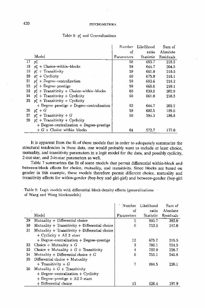
Table 8: p~ and Generalizations

Model17 p;18 p~ + Choice-within-blocks19 p~ + Transitivity20 p~ + Cyclicity21 p~ + Degree-centralization22 p~ + Degree-prestige23 p~ + Transitivity + Choice-within-blocks24 p~ + Transitivity + Cyclicity25 p~ + Transitivity + Cyclicity

+ Degree-prestige + Degree-centralization26 p~ + G27 p~ + Transitivity + G28 p~ + Transitivity + Cyclicity

+ Degree-centralization + Degree-prestige+ G + Choice-within-blocks

Number Likelihood Sum ofof ratio Absolute

Parameters Statistic Residuals58 683.7 218.559 644.7 204.559 661.0 210.560 675.9 216.159 683.6 218.359 668.0 210.160 639.5 202.960 661.0 210.5

62 644.7 202.259 602.5 189.060 595.3 186.8

64 572.7 177.0

It is apparent from the fit of these models that in order to adequately summarize thestructural tendencies in these data, one would probably want to include at least choice,mutuality, and transitivity parameters in a logit model for the data, and possibly cyclicity,2-out-star, and 2-in-star parameters as well.

Table 7 summarizes the fit of some models that permit differential within-block andbetween-block effects for choice, mutuality, and transitivity. Since blocks are based ongender in this example, these models therefore permit different choice, mutuality andtransitivity effects for within-gender (boy-boy and girl-girl) and between-gender (boy-girl

T̄able 9: Logit models with differential block-density effects (generalizationsof Wang and Wong blockmodels)

Model29 Mutuality + Differential choice30 Mutuality + Transitivity + Differential choice31 Mutuality + Transitivity + Differential choice

+ Cyclicity + All 2-stars+ Degree-centralization + Degree-prestige

32 Choice + MutuMity + G33 Choice + Mutuality + G + Transitivity34 Mutuality + Differential choice + G35 Differential choice + Mutuality

+ Transitivity + G36 Mutuality + G + Transitivity

+ Degree-centralization + Cyclicity+ Degree-prestige + All 2-stars+ Differential choice

Number Likelihood Sum ofof ratio Absolute

Parameters Statistic Residuals5 895.7 302.06 753.0 247.0

12 675.7 215.53 780.1 254.54 702.9 226.76 755.1 245.8

7 684.5 220.1

13 626.4 197.9

STANLEY WASSERMAN AND PHILIPPA PATrlSON 421

Table 10: General differential block effects (based on gender)

Model37 Choice + Differential mutuality38 Choice + Mutuality

+ Differential degree-prestige39 Choice + Mutuality

+ Differential degree-centralization40 Differential mutuality + Differential choice41 Differential mutuality + Differential choice

+ Transitivity42 Choice + Mutuality + Differential transitivity43 Mutuality + Differential transitivity

+ Differential choice44 Differential choice + Differential mutuality

+ Differential transitivity45 Differential mutuality + Differential choice + G46 Mutuality + Differential choice

+ Differential within-block transitivity47 Differential choice + Differential mutuality + G

+ All 2-stars + Degree-prestige+ Transitivity

48 Differential choice + Mutuality + Transitivity+ Differential within-block transitivity

Number Likelihood Sum ofof ratio Absolute

Parameters Statistic Residuals5 935.5 315.2

4 967.8 330.6

4 948.1 322.48 887.0 299.3

9 744.6 244.26 748.7 244.6

9 739.8 243.1

12 729.0 240.09 735.9 239.1

7 831.0 275.6

16 610.1 193.4

8 751.0 245.7

and girl-boy) ties. Comparing Models 14 through 16 with Model 3, we see a modesttendency for stronger within-block choice effects, but only small tendencies for strongerwithin-block reciprocity and transitivity.

The models summarized in Table 8 include p ~ and various generalizations. Model 18adds a single within-block choice parameter to Model 17, with a reasonable increase in fit.This model is a logit formulation of a stochastic blockmodel in which block effects are all

¯ equal and occur only on the diagonal of the blockmodel. Models 19 through 25 augmentp~ with one or more other structural parameters, but Model 18 appears to provide one ofthe more useful improvements in fit overp]. Models 26 through 28 illustrate how differentdensity effects can be fitted in the presence and absence of another relation (the "WorkWith" relation). The parameter ~/corresponds to a graph statistic (G) that is a count of number of pairs of nodes joined by both "Work With" and "Get on With" ties, and soreflects the greater likelihood of a "Get on With" tie in the presence of a "Work With" tie.

We also considered models with differential choice effects according to the gender ofthe sender and recipient of a tie (see Table 9). Model 29 specifies a mutuality effect anddifferent choice parameters for each of these four types of tie (boy-boy, boy-girl, girl-boy,girl-girl). It is a better fit than Model 2, suggesting that the likelihood of ties varies amongand between blocks. Model 30 adds a transitivity parameter to Model 2, while Model 31adds various other homogeneous effects as well. Models 32 through 36 add a parameter forassociation with the "Work With" .relation. It may be noted that Model 30 appears toprovide a better fit to the data than Model 15; thus, the model that constrains within-gender effects to be equal (that is, boy-boy and girl-girl) and between-gender effects to equal (that is, boy-girl and girl-boy) does not provide as good a fit to the data as the model

0

z

424 PSYCHOMETRIKA

in much of modern applied statistics (for example, with covariance structure models andtest theory). Further investigation of the quality of maximum pseudolikelihood estimatesis certainly called for, and will be the topic of future research.

Comparisons ofpl-type models and the ML estimates of their parameters with logitp* models and their approximate, MP parameter estimates have been made by Strauss andIkeda (1990). We have also investigated how much is "lost" in MP estimation in very smallnetworks (Walker, 1995). The bottom line from this initial research (which is quite assuring) is that approximate MP estimates are quite close to their exact, ML counterparts.We can proceed to postulatep*-type models, and fit them approximately, and probably notlose too much in the process (over exact estimation).

These preliminary results will certainly be augmented in the future, particularly sincethe advent of computationally-intensive ML estimation techniques (such as the Gibbssampler and Markov chain Monte Carlo ideas) should make ML estimation more feasible.

In spite of this approximate estimation approach, the models and estimation strategyproposed here have substantial benefits. This approach has tremendous flexibility to ex-press plausible and interesting structural assumptions, coupled with ease in model fitting.

There is more to be done to generalize these models to other types of relations.Pattison and Wasserman (in press) describe some of these extensions, to valued andbivariate relations.

References

Agresti, A. (1990). Categorical data analysis. New York: John Wiley and Sons.Anderson, C. J., & Wasserman, S. (1995). Logrnultilinear models for valued social relations. Sociological Methods

& Research, 24, 96-127.Besag, J. (1974). Spatial interaction and the statistical analysis of lattice systems. Journal of the Royal Statistical

Society, Series B, 36, 192-236.Faust, K., & Wasserman, S. (1992). Centrality and prestige: A review and synthesis. Journal of Quantitative

Anthropology, 4, 23-78.Fienberg, S. E. (1980). The analysis of cross-classified, categorical data (2nd ed.). Cambridge, MA: The MIT Press.Fienberg, S. E., & Wasserman, S. (1981). Categorical data analysis of single sociometric relations. In S. Leinhardt

(Ed.), Sociological methodology 1981 (pp. 156-192). San Francisco: Jossey-Bass.Frank, O., & Strauss, D. (1986). Markov random graphs. Journal of the American Statistical Association, 81,

832-842.Holland, P. W., & Leinhardt, S. (1973). The structural implications of measurement error in sociometry. Journal

of Mathematical Sociology, 3, 85-111.Holland, P. W., & Leinhardt, S. (1975). The statistical analysis of local structure in social networks. In D. R. Heise

(Ed.), Sociological methodology 1976 (pp. 1-45). San Francisco: Jossey-Bass.Holland, P. W., & Leinhardt, S. (1977). Notes on the statistical analysis of social network data. Unpublished

.manuscript.Holland, P. W., & Leinhardt, S. (1978). An omnibus test for social structure using triads. Sociological Methods &

Research, 7, 227-256.Holland, P. W., & Leinhardt, S. (1979). Structural sociometry. In P. W. Holland & S. Leinhardt (Eds.), Perspec-

tives on social network research (pp. 63-83). New Y~rk: Academic Press.Holland, P. W., & Leinhardt, S. (1981). An exponential family of probability distributions for directed graphs.

Journal of the American Statistical Association, 76, 33-65. (with discussion)Iacobucci, D., & Wasserman, S. (1990). Social networks with two sets of actors. Psychometrika, 55, 707-720.Ising, E. (1925). Beitrag zur theorie des ferramagnetismus. Zeitschrift fur Physik, 31,253-258.Johnsen, E. C. (1985). Network macrostructure models for the Davis-Leinhardt set of empirical sociomatrices.

Social Networks, 7,. 203-224.Johnsen, E. C. (1986). Structure and process: Agreement models for friendship formation. Social Networks, 8,

257-306.Kindermann, R. P., & Snell, J. L. (1980). On the relation between Markov random fields and social networks.

Journal of Mathematical Sociology, 8, 1-13.Koehly, L., & Wasserman, S. (1994). Classification of actors in a social network based on stochastic centrality and

prestige. Manuscript submitted for publication.

STANLEY WASSERMAN AND PHILIPPA PATTISON 425

Pattison, P., & Wasserman, S. (in press). Logit models and logistic regressions for social networks: II. Extensionsand generalizations to valued and bivariate relations. Journal of Quantitative Anthropology.

Reitz, K. P. (1982). Using log linear analysis with network data: Another look at Sampson’s monastery. SocialNetworks, 4, 243-256.

Ripley, B. (1981). Spatial statistics. New York: Wiley.Sampson, S. F. (1968). A novitiate in a period of change: An experimental and case study of relationships. Unpub-

lished doctoral dissertation, Department of Sociology, Cornell University, Ithaca, NY.Snijders, T. A. B. (1991). Enumeration and simulation methods for 0-1 matrices with given marginals. Psy-

chometrika, 56, 397-417.Speed, T. P. (1978). Relations between models for spatial data, contingency tables, and Markov fields on graphs.

Supplement Advances in Applied Probability, 10, 111-122.Strauss, D. (1977). Clustering on colored lattices. Journal of Applied Probability, 14, 135-143.Strauss, D. (1986). On a general class of models for interaction. SIAM Review, 28, 513-527.Strauss, D. (1992). The many faces of logistic regression. The American Statistician, 46, 321-327.Strauss, D., & Ikeda, M. (1990). Pseudolikelihood estimation for social networks. Journal of the American

Statistical Association, 85, 204-212.Vickers, M. (1981). Relational analysis: An applied evaluation. Unpublished Masters of science thesis, Department

of Psychology, University of Melbourne, Australia.Vickers, M., & Chan, S. (1981). Representing classroom social structure. Melbourne: Victoria Institute of Second-

ary Education.Walker, M. E. (1995). Statistical models for social support networks: Application of exponential models to undirected

graphs with dyadic dependencies. Unpublished doctoral dissertation, University of Illinois, Department ofPsychology.

Wang, Y. J., & Wong, G. Y. (1987). Stochastic blockmodels for directed graphs. Journal of the American StatisticalAssociation, 82, 8-19.

Wasserman, S. (1978). Models for binary directed graphs and their applications. Advances in Applied Probability,10, 803-818.

Wasserman, S. (1987). Conformity of two sociometric relations. Psychometrika, 52, 3-18.Wasserman, S., & Faust, K. (1994). Social network analysis: Methods and applications. Cambridge, England:

Cambridge University Press.Wasserman, S., & Galaskiewicz, J. (1984). Some generalizations ofpl: External constraints, interactions, and

non-binary relations. Social Networks, 6, 177-192.Wasserman, S., & Iacobucci, D. (1986). Statistical analysis of discrete relational data. British Journal of Mathe-

matical and Statistical Psychology, 39, 41-64.

Manuscript received 1/20/95Final version received 6/6/95