Logistics clustering in space? A study on economies of

agglomeration in Noord-Brabant

Robin Navis, January 2020

Abstract: This Master’s thesis studies the effect of economies of agglomeration on rents of logistics

real estate in Noord-Brabant. Economies of agglomeration may occur when same industry firms co-

locate or cluster together in order to benefit from each other. These firms that cluster may experience

a positive effect on their productivity due to economies of agglomeration. Three main sources are

described which are labour market pooling, input sharing, and knowledge spillovers. In their own way,

these sources can all effect logistics firms. For example, lower costs can be achieved when logistics

firms combine their transport flows or exchange knowledge. In order to understand the implications

of economies of agglomeration in the logistics sector, this paper tries to indicate and measure these

economies in the province Noord-Brabant. The Strabo and LISA databases are used in this research.

The Strabo database provides data of rental transactions of logistics properties from 1989 to 2017. The

LISA database contains employment numbers of multiple commercial properties per year. The effects

of economies of agglomeration are indicated and estimated by using multiple hedonic pricing models.

Herewith, the effect of property/locational characteristics, infrastructural characteristics, and job

concentration indices on the rents per square meter will be clarified. The results of the research

indicate that higher rents occur in areas with higher population densities, due to the fact that the

proximity of customers will lower transport costs as it also helps to create a local network. In

predefined rural areas rents are respectively 14.19% and 17.96% lower than in the denser urban areas.

Also, the distance to the highway entrance only impacts rents of smaller (<2,500 m²) firms, with

changes of rents per kilometre to -2.51%. Lastly, with the use of the LISA database and the Herfindahl-

Hirschman index the concentration indices like the Ellison-Glaeser index and the Location Quotient

were constructed. While the Ellison-Glaeser index is somewhat more complex compared to the

Location Quotient, both indices are based on standard concentration ratios and can be constructed

with readily available data. The Ellison-Glaeser index defines concentration as agglomeration above

and beyond what we would observe if establishments/firms simply chose locations randomly. Of these

concentrations the Ellison-Glaeser index has a significant effect on the rents of logistics real estate.

When the Ellison-Glaeser index rises by ten points the rents per square meter increase by 3.6%,

indicating that in regions where localization of firms are beyond that expected by pure randomness,

the rents increase. Carefulness is required however. Because the significance is based on a 90% level,

the impact can be considered less reliable than to be preferred. Also, the Location-Quotient was not

significantly different from zero in any model on all significance levels, indicating no impact of clustered

jobs on the property rents.

Keywords: economies of agglomeration, logistics real estate, Noord-Brabant, hedonic modelling, job

concentration indices.

2

Colophon

Title: Logistics clustering in space? A study on economies of agglomeration in

Noord-Brabant

Version: Master Thesis

Author: Robin Navis

Address: Tweede Beuzenes 11

7101 WB Winterswijk

Student number: S3279103

Telephone: +31 (0)6 11 86 26 84

E-mail: r.navis@student.rug.nl

Supervisor: M.N. Daams

Master: MSc Real Estate Studies

Faculty: Faculty of Spatial Sciences

Disclaimer: “Master theses are preliminary materials to stimulate discussion and critical comment.

The analyses and conclusions set forth are those of the author and do not indicate concurrence by

the supervisor or research staff.”

3

Table of contents

1. Introduction…………………………………………………………………………………………………….. 4

2. Theoretical Framework……………………………………………………………………………………. 6

2.1 Economies of agglomeration……………………………………………………………….. 6

2.2 Logistics Clustering………………………………………………………………………………. 7

2.3 Hypotheses………………………………………………………………………………………….. 9

3. Data & Methodology……………………………………………………………………………………….. 9

3.1 Study Area…………………………………………………………………………………………… 9

3.2 Dataset……………………………………………………………………………………………….. 10

3.3 Empirical Model………………………………………………………………………………….. 11

3.4 Variables……………………………………………………………………………………………… 12

3.4.1 Property characteristics…………………………………………………………… 12

3.4.2 Locational characteristics………………………………………………………… 12

3.4.3 Infrastructural characteristics………………………………………………….. 14

3.4.4 Jobs concentration characteristics ………………………………………….. 14

3.4.5 Fixed effects……………………………………………………………………………. 16

3.5 Variables description…………………………………………………………………………… 16

4. Results…………………………………………………………………………………………………………….. 19

5. Discussion……………………………………………………………………………………………………….. 24

5.1 Company size and economies of agglomeration…………………………………… 24

5.2 Concentration of jobs and economies of agglomeration………………………. 24

5.3 Data limitations and further research………………………………………………….. 25

6. Conclusion………………………………………………………………………………………………………. 25

References…………………………………………………………………………………………………………….. 27

Appendix I…………………………………………………………………………………………………………….. 31

Appendix II……………………………………………………………………………………………………………. 33

Appendix III…………………………………………………………………………………………………………… 35

4

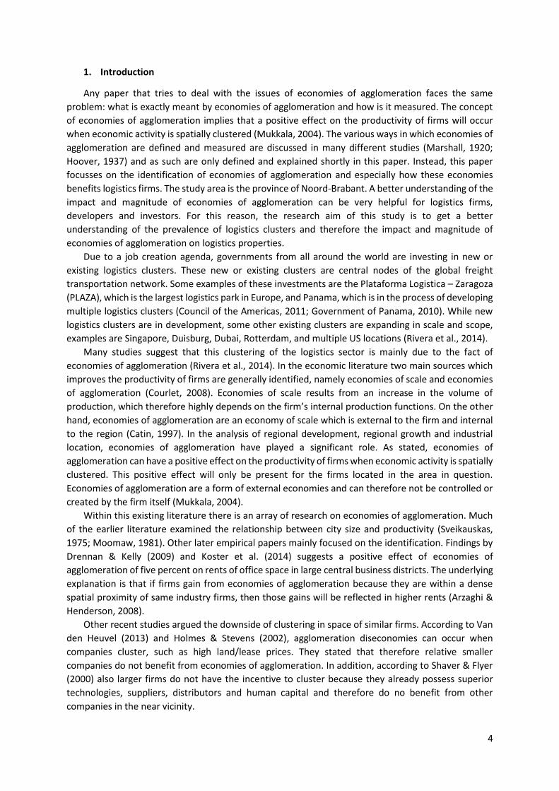
1. Introduction

Any paper that tries to deal with the issues of economies of agglomeration faces the same

problem: what is exactly meant by economies of agglomeration and how is it measured. The concept

of economies of agglomeration implies that a positive effect on the productivity of firms will occur

when economic activity is spatially clustered (Mukkala, 2004). The various ways in which economies of

agglomeration are defined and measured are discussed in many different studies (Marshall, 1920;

Hoover, 1937) and as such are only defined and explained shortly in this paper. Instead, this paper

focusses on the identification of economies of agglomeration and especially how these economies

benefits logistics firms. The study area is the province of Noord-Brabant. A better understanding of the

impact and magnitude of economies of agglomeration can be very helpful for logistics firms,

developers and investors. For this reason, the research aim of this study is to get a better

understanding of the prevalence of logistics clusters and therefore the impact and magnitude of

economies of agglomeration on logistics properties.

Due to a job creation agenda, governments from all around the world are investing in new or

existing logistics clusters. These new or existing clusters are central nodes of the global freight

transportation network. Some examples of these investments are the Plataforma Logistica – Zaragoza

(PLAZA), which is the largest logistics park in Europe, and Panama, which is in the process of developing

multiple logistics clusters (Council of the Americas, 2011; Government of Panama, 2010). While new

logistics clusters are in development, some other existing clusters are expanding in scale and scope,

examples are Singapore, Duisburg, Dubai, Rotterdam, and multiple US locations (Rivera et al., 2014).

Many studies suggest that this clustering of the logistics sector is mainly due to the fact of

economies of agglomeration (Rivera et al., 2014). In the economic literature two main sources which

improves the productivity of firms are generally identified, namely economies of scale and economies

of agglomeration (Courlet, 2008). Economies of scale results from an increase in the volume of

production, which therefore highly depends on the firm’s internal production functions. On the other

hand, economies of agglomeration are an economy of scale which is external to the firm and internal

to the region (Catin, 1997). In the analysis of regional development, regional growth and industrial

location, economies of agglomeration have played a significant role. As stated, economies of

agglomeration can have a positive effect on the productivity of firms when economic activity is spatially

clustered. This positive effect will only be present for the firms located in the area in question.

Economies of agglomeration are a form of external economies and can therefore not be controlled or

created by the firm itself (Mukkala, 2004).

Within this existing literature there is an array of research on economies of agglomeration. Much

of the earlier literature examined the relationship between city size and productivity (Sveikauskas,

1975; Moomaw, 1981). Other later empirical papers mainly focused on the identification. Findings by

Drennan & Kelly (2009) and Koster et al. (2014) suggests a positive effect of economies of

agglomeration of five percent on rents of office space in large central business districts. The underlying

explanation is that if firms gain from economies of agglomeration because they are within a dense

spatial proximity of same industry firms, then those gains will be reflected in higher rents (Arzaghi &

Henderson, 2008).

Other recent studies argued the downside of clustering in space of similar firms. According to Van

den Heuvel (2013) and Holmes & Stevens (2002), agglomeration diseconomies can occur when

companies cluster, such as high land/lease prices. They stated that therefore relative smaller

companies do not benefit from economies of agglomeration. In addition, according to Shaver & Flyer

(2000) also larger firms do not have the incentive to cluster because they already possess superior

technologies, suppliers, distributors and human capital and therefore do no benefit from other

companies in the near vicinity.

5

Despite many different studies on economies of agglomeration, there is limited insights of these

economies in the logistics sector. According to Mukkala (2004) logistics firms can also improve their

productivity or lower production costs when benefitting from economies of agglomeration and

thereby creating an advantage over their competitors. Most studies that are focused on logistics,

support this claim by Mukkala (2014) and argue that logistics clusters, just as other clusters, will benefit

from agglomeration economies (Van den Heuvel et al., 2013; Koster et al., 2014; Rivera et al., 2016).

Some other authors even say that in regions where these clusters are located higher economic growth

and higher rate of innovation will occur than in regions without clusters (Porter, 2000; Delgado et al.,

2010). Lastly, big government investments in logistics clusters could suggests that policy makers are

indeed acknowledging the positive effects of economies of agglomeration when same industry firms

do cluster (Kasarda, 2008; Wu et al., 2006).

There are multiple approaches of measuring economies of agglomeration. The most common way

is to directly estimate the production function. In carrying out this estimation, multiple inputs such as

numbers of employment, capital, materials and land are necessary (Rosenthal & Strange, 2002). A

different approach is with the focus on births of new establishments and their employment. The idea

of this approach is that entrepreneurs seek out the most productive regions and therefore chose the

locations which will maximize their profit (Carlton, 1983). A third approach is to study differences in

wages. With this approach the assumption is made that labour is paid the value of its marginal product

in competitive markets. The last approach to measure economies of agglomeration is with the use of

property rents (Rosenthal & Strange, 2002). This approach, to use rents, will be used in this thesis,

mainly due to the availability of data necessary and available. Very few studies use rents in order to

measure the presence of agglomeration economies. Still some have shown that agglomeration

economies mainly capitalize in rents (Koster et al., 2014; Arzaghi & Henderson, 2008; Drennan & Kelly,

2009). The approach to use rents stems from the quality-of-life literature and means: “if firms are

paying higher rents in a particular location all else equal, then the location must have some

compensating productivity differential (Rosenthal & Strange, 2005).“ Rents of logistics properties

should be higher when co-locating with same industry firms due to different advantages such as an

increased productivity, easier access to information, ease of new business formation, new

technological and delivery possibilities, and benefits rooted in working together with other institutions

such as universities and public organizations (Rivera et al., 2016; Porter, 1998). In addition, this study

will focus on the external localization economies of logistic firms. Localization economies is

characterized by the geographical concentration of a specific industry, in this case logistics. The

external economies of scale depend on the development of the whole industry in the region. In the

next chapter, these different sources of economies of agglomeration are further explained.

This paper contributes to the understanding of agglomeration economies when logistics firms are

spatially clustered. To link economies of agglomeration to logistics property rents, logistics rental

transaction data from 1989-2017 in the province Noord-Brabant are examined (N=511). In this paper

the following research question will be answered:

“To what extent does spatially clustering of logistics firms create economies of agglomeration in the

province of Noord-Brabant?”

To answer this question and test the effects of clustering in space on logistics property rents, this

paper uses hedonic pricing models. Hedonic price modelling is a statistical method, which values

location-specific amenities by measuring the price differentials (Hoehn et al., 1987). By applying

multiple linear regressions, the effects of co-locating can be identified and measured. Also, other

attributes comprising property-, locational- and infrastructural characteristics are plotted in the linear

regression in order to measure their effects on logistics property rents.

6

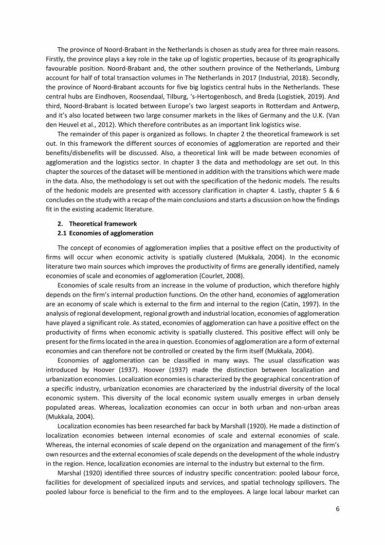
The province of Noord-Brabant in the Netherlands is chosen as study area for three main reasons.

Firstly, the province plays a key role in the take up of logistic properties, because of its geographically

favourable position. Noord-Brabant and, the other southern province of the Netherlands, Limburg

account for half of total transaction volumes in The Netherlands in 2017 (Industrial, 2018). Secondly,

the province of Noord-Brabant accounts for five big logistics central hubs in the Netherlands. These

central hubs are Eindhoven, Roosendaal, Tilburg, ‘s-Hertogenbosch, and Breda (Logistiek, 2019). And

third, Noord-Brabant is located between Europe’s two largest seaports in Rotterdam and Antwerp,

and it’s also located between two large consumer markets in the likes of Germany and the U.K. (Van

den Heuvel et al., 2012). Which therefore contributes as an important link logistics wise.

The remainder of this paper is organized as follows. In chapter 2 the theoretical framework is set

out. In this framework the different sources of economies of agglomeration are reported and their

benefits/disbenefits will be discussed. Also, a theoretical link will be made between economies of

agglomeration and the logistics sector. In chapter 3 the data and methodology are set out. In this

chapter the sources of the dataset will be mentioned in addition with the transitions which were made

in the data. Also, the methodology is set out with the specification of the hedonic models. The results

of the hedonic models are presented with accessory clarification in chapter 4. Lastly, chapter 5 & 6

concludes on the study with a recap of the main conclusions and starts a discussion on how the findings

fit in the existing academic literature.

2. Theoretical framework

2.1 Economies of agglomeration

The concept of economies of agglomeration implies that a positive effect on the productivity of

firms will occur when economic activity is spatially clustered (Mukkala, 2004). In the economic

literature two main sources which improves the productivity of firms are generally identified, namely

economies of scale and economies of agglomeration (Courlet, 2008).

Economies of scale results from an increase in the volume of production, which therefore highly

depends on the firm’s internal production functions. On the other hand, economies of agglomeration

are an economy of scale which is external to the firm and internal to the region (Catin, 1997). In the

analysis of regional development, regional growth and industrial location, economies of agglomeration

have played a significant role. As stated, economies of agglomeration can have a positive effect on the

productivity of firms when economic activity is spatially clustered. This positive effect will only be

present for the firms located in the area in question. Economies of agglomeration are a form of external

economies and can therefore not be controlled or created by the firm itself (Mukkala, 2004).

Economies of agglomeration can be classified in many ways. The usual classification was

introduced by Hoover (1937). Hoover (1937) made the distinction between localization and

urbanization economies. Localization economies is characterized by the geographical concentration of

a specific industry, urbanization economies are characterized by the industrial diversity of the local

economic system. This diversity of the local economic system usually emerges in urban densely

populated areas. Whereas, localization economies can occur in both urban and non-urban areas

(Mukkala, 2004).

Localization economies has been researched far back by Marshall (1920). He made a distinction of

localization economies between internal economies of scale and external economies of scale.

Whereas, the internal economies of scale depend on the organization and management of the firm’s

own resources and the external economies of scale depends on the development of the whole industry

in the region. Hence, localization economies are internal to the industry but external to the firm.

Marshal (1920) identified three sources of industry specific concentration: pooled labour force,

facilities for development of specialized inputs and services, and spatial technology spillovers. The

pooled labour force is beneficial to the firm and to the employees. A large local labour market can

7

protect firms and workers from demand-shocks and business uncertainty. In perspective of the firms,

recruitment costs will be lower because of this pool of highly skilled workers. Second, the proximity of

customers and suppliers helps to create a local network conducive to economic growth and more

effective production. High local demand allows producers of intermediate inputs to break-even. This

will increase the variety of intermediate goods, which in turn will make the production of the final

product more efficient (Mukkala, 2004). Finally, the spatial technology spillovers or knowledge

spillovers can also be very beneficial for a firm. Knowledge and ideas about production or new products

can be transferred between firms by imitation, inter-firm circulation of employees, business

interactions, or by informal exchanges (Saxenian, 1994). The larger the number of workers in a certain

industry will create a higher opportunity to exchange knowledge (Henderson, 1986).

In addition to the benefits above from clustering in space, other authors identified disbenefits

(Bounie & Blanquart, 2017). Firstly, economies of agglomeration can lead to pressure on the price of

land and property, when there is a fixed physical supply (Fujita & Krugman, 2004). Next, due to

concentration of economic activity higher sources of pollution will occur (Feitelson & Salomon, 2000).

Also, the higher efficiency of supply chains could diminish the advantage of geographical proximity,

leading to negative externalities of clusters (Cairncross, 1997; Henderson & Shalizi, 2001). Last, the

matching of resources sometimes fails to materialize. For example, specialized workers may be easier

to find by firms due to concentration, but this could also lead to tensions regarding the workforce,

resulting in increased wages and volatility (Chatterjee, 2003).

As stated above, the different sources of economies of agglomeration can have important

implications for a firm’s location strategy, as a source of reduced costs. Firms will have an advantage

over competitors when benefitting from economies of agglomeration. Whether a firm does benefit

from economies of agglomeration depend on different issues. First, the factors of agglomeration have

different values to different firms. Second, both firm and agglomeration economy heterogeneity will

impact the value of an economy of agglomeration. In the next sector, a linkage is made between

economies of agglomeration and the logistics sector.

2.2 Logistics clustering

Logistics real estate is one of the main asset classes of commercial property. A classification of the

definition of logistics as ‘business’ and as ‘real estate’ is essential for a better understanding of the

nature of the logistics market. Logistics as a business can be defined as “the process of planning,

implementing, and controlling procedures for the efficient and effective transportation and storage of

goods including services, and related information from the point of origin to the point of consumption

for the purpose of conforming to customer requirements (Mattarocci & Pekdemir, 2017).” Logistics as

in a real estate asset can be seen as the distribution and storage purpose-built buildings used for the

process mentioned above.

In the last decade, the European industrial and logistics market has changed vastly. Two major

phenomena had a huge impact in changing demand and supply dynamics and therefore shaping the

market. These two phenomena are industrial and technological revolutions. The industrial market has

undergone a progressive development over the last hundred years and has entered a new phase with

changing consumption patterns and global trade (Mattarocci & Pekdemir, 2017). Since late nineteenth

century the modern industrial market has been growing. Industrial areas agglomerated around

transportation nodes, during the 1920s and 1930s. However, since the 1950s both distribution and

manufacturing industries have been decentralized. The improved infrastructure providing accessibility

to areas outside of the big cities was one of the many factors contributing to the suburbanization of

the industry. Later, technological innovation and globalization impacted the development of the

industrial market (Peiser and Schwanke, 1992).

8

The increasingly clustering of logistics activities has led some researchers to examine economies

of agglomeration attributed to these logistics clusters. Marshall (1920) described three main sources

of economies of agglomeration, namely labour market pooling, input sharing, and knowledge

spillovers. First, labour market pooling can provide firms, which co-locate, a better access to a more

flexible labour market, specialized labour, and better training. When addressing logistics firms, these

benefits are usually only beneficial when firms operate in different supply chains, since they serve

different markets (Van den Heuvel et al., 2012). Second, Marshall (1920) also mentioned input sharing,

which relates to the broad local supplier base, that increases flexibility and reduces costs. Input sharing

can be beneficial in the logistics sector in different ways. First, lower transport costs can be achieved

when logistics firms that co-locate combine their transport flows. According to Jara-Díaz & Basso

(2003) cooperation between co-located transport firms can result in lower transport costs due to a

denser network, a decrease in empty mileage (Cruijssen et al., 2007a), less repositioning of trucks

(Ergun et al., 2007), and a decrease in the distance between customers (Van Donselaar et al., 1999;

Wouters et al., 1999), which subsequently also has a positive environmental impact (Van den Heuvel

et al., 2012). Also, co-location may lead to supply of storage capacity by third parties, due to (short-

term) demand of several firms. Last, multimodal transport could be possible due to an increase of

freight volumes. Multimodal transport can’t compete with road transport because of insufficient large

freight volumes. An increase in freight volumes could enable the development of multimodal transport

services, when logistics firms co-locate (Van den Heuvel et al., 2012). Also, Rivera et al., (2014) stated

that firms in logistics clusters lease space to each other for short-term surges, share equipment, work

together effectively when contracts are being moved from provider.

Third, Marshall (1920) refers to knowledge spillovers, which idea is that geography plays a

fundamental role in learning and innovation. Collaboration of different firms are usually the starting

point of innovation, and, when the distance increases between firms the cost of exchanging

information also increases, all else equal (Malmberg & Maskell, 1997). According to Lasserre (2008),

this is mainly because of the need to create trust and understanding between firms, which in turn

depends on culture, language and shared values. According to Malmberg & Maskell (2002), the starting

point of many spatial agglomerations are the spatial attributes of interactive learning and innovation

processes. However, localized knowledge may be less relevant in the logistics sector given the fact that

knowledge management hasn’t been largely implemented by logistics firms (Neumann & Tomé, 2005).

Still, according to Cruijssen et al. (2007b) the difficulty of finding a trusted party is one of the important

impediments for horizontal cooperation in logistics. To overcome this impediment, co-location may

help. Furthermore, clustered firms have more weight in lobbying for improved infrastructure and

regulatory relief with the local government (Rivera et al., 2014).

Other authors highlighted the importance of accessibility and general infrastructure as the main

factor for logistics clusters (Bok, 2009). According to Berechman (1994), a better accessibility drives

logistics operations to cluster together, as it also reduces costs (Rietveld, 1994). For foreign logistics

firms, the transportation accessibility is one of the important determinants considering location (Hong,

2007).

On the other hand, some scholars say the effects of economies of agglomeration when logistics

activities are concentrated should not be overstated. According to Carbonara et al. (2002) there is a

lack of interfirm relations in industry districts, referring to Dell’Orco et al. (2009) who stated that the

companies mostly behave as individual agents in a cluster and that they usually don’t know the other

firms at near distance. Masson & Petiot (2014) had the same conclusion in their empirical study of the

situation in France, which stated that there was an absence of the externalities explained by Marhall

(1920) (knowledge spillovers, input sharing, and labour pooling), and on the contrary a presence of

diseconomies. They partly explained this due to the high concentration of low-skilled workers, resulted

due to logistics activities, which will unlikely lead to knowledge spillovers.

9

Another recent study argued the downside of clustering in space of similar firms. According to

Shaver & Flyer (2000) some firms may have greater benefits than others regarding economies of

agglomeration. Firms which already possess superior technologies, suppliers, distributors and human

capital do not have the incentive to locate close to other same industry firms. These firms will not only

capture the benefits but also contribute to agglomeration economies. Resulting, larger firms (relative

to average establishment size in industry) are less likely to agglomerate, their presence would increase

local economic activity which then could result in lower costs for neighbouring competitors (Shaver &

Flyer, 2000). Also, Alcácer & Chung (2007) argued that whether competitors can absorb economies of

agglomeration, especially knowledge spillovers. It is crucial for these knowledge spillovers that they

can be absorb by smaller firms. Industry leaders will otherwise freely benefit from agglomeration when

competitors can’t leverage the knowledge they gather from the larger and more technically advanced

firms.

2.3 Hypotheses

Based on the theoretical framework, three hypotheses are formed:

Hypothesis 1: logistics firms pay a significant higher property rent when located near infrastructure

nodes. This hypothesis is based on the importance of accessibility and general infrastructure some

authors highlight. A better accessibility drives logistics operations to cluster together, this could reduce

the costs of transport (Berechman, 1994; Rietveld, 1994).

Hypothesis 2: due to possible economies of agglomeration logistics firms pay a significant higher

property rent when clustered. These economies of agglomeration will be based on the density and

clustering of logistics employment. The increasingly clustering of logistics activities has led researchers

to examine economies of agglomeration attributed to these logistics clusters. Marshall (1920)

described three main sources of economies of agglomeration, namely labour market pooling, input

sharing, and knowledge spillovers. In their own way, these sources can all effect logistics firms and

lower their production costs.

Hypothesis 3: the company size has a significant effect on the benefits of economies of agglomeration

implying economies at firm-level. According to Shaver & Flyer (2000) some firms may have greater

benefits than others regarding economies of agglomeration. Firms which already possess superior

technologies, suppliers, distributors and human capital do not have the incentive to locate close to

other same industry firms. Resulting, larger firms are less likely to agglomerate. Also, it is crucial

whether firms can absorb economies of agglomeration. Bigger firms will freely benefit when the

smaller competitors can’t leverage the knowledge gathered from the larger and more technically

advanced firms.

3. Data & Methodology

3.1 Study area

In figure 3.1 the study area is shown, the logistics transaction over the years (1989-2017) are linked

to the blue dots (N=511). Furthermore, the borders are shown of the province and COROP-regions.

Lastly, the hard infrastructure such as the highway and train tracks are presented. The study

concentrates on Noord-Brabant. Noord-Brabant is a province in the south of The Netherlands and is

chosen as study area for multiple reasons:

10

Figure 3.1: Study area including plotted observations.

Firstly, the province plays a key role in the take up of logistic properties, because of its

geographically favourable position. Noord-Brabant and Limburg account for half of total logistics

transaction volumes in The Netherlands in 2017 (Industrial, 2018). Secondly, the province of Noord-

Brabant accounts for five big logistics central hubs in the likes of Eindhoven, Roosendaal, Tilburg, ‘s-

Hertogenbosch, and Breda. And lastly, Noord-Brabant is located between Europe’s two largest

seaports in Rotterdam and Antwerp and the U.K.’s and Germany’s large consumer markets (Van den

Heuvel et al., 2012). These reasons make the province of Noord-Brabant an ideal province for

measuring effects of agglomeration economies.

3.2 Dataset

The hypotheses in this study are tested using secondary data from multiple sources. The datasets

that were used are the Strabo commercial real estate database and the LISA database employment

register. Furthermore, data regarding infrastructure is obtained with the use of ArcGis and a report

from the Ministry of Infrastructure and Water Management. The construction year and locational

characteristics, such as the surface and growth of the business park, were obtained from the Dutch

land registry office.

The Strabo commercial real estate database contains of rental and asset transactions for individual

properties at the time of purchase between 1989 and 2017, which includes multiple periods of both

boom and bust in the commercial real estate market. The rental transactions of the database were

11

used due to the fact that these could indicate potential economies of agglomeration. In the Strabo

database information was given per transaction, this includes rents, surface, transaction date, existing

or new build, tenant type, and postal codes with addresses.

The LISA database employment register contains employment numbers of multiple commercial

properties between 1995 and 2016. In the LISA database information was given on the total jobs per

address for every year. The database was also used in order to calculate the number of jobs in a specific

region (municipality and province) per year.

These two datasets were combined in order to match the property characteristics with the job

characteristics on property level. Because the LISA database only contained data till 1995, the

transaction in the Strabo database from 1989 to 19941 were also matched with the job characteristics

from 1995. Combining the Strabo database (< 5,500 logistics transactions) and LISA database (<

6,000,000 cases), and further stratification by property type (logistic), study area (Noord-Brabant),

property status (rental), surface (< 500m2), duplicates, outliers, and missing data, reduced the final

sample to 511 observations.

Furthermore, data on locational characteristics regarding the business park were obtained from

the Dutch land registry office. The Dutch land registry office (CBS) keeps track of different land uses in

the Netherlands since the 1940s. In this thesis we use the category business park to construct the

surface and growth of the area where the particular transaction took place. With the data from CBS

we can map the land uses per year and calculate, with the use of ArcGis, the surface and the growth

of the business parks. In this thesis we only got land use data from the years 1996, 2000, 2003, 2010,

and 2015. Some years could not be used because of some minor errors in the data

To summarize, the 511 observations are rental transactions of logistic properties in Noord-Brabant

in the time period between 1989 and 2017. The transactions contain data with property-, locational-,

infrastructure- and job characteristics.

3.3 Empirical Model

To test the effects of economies of agglomeration on logistics rents, multiple hedonic models are

set-up. Hedonic price modelling is a statistical method, which values location-specific amenities by

measuring the price differentials. The basic concept is as follows: if individuals are to locate in

undesirable and desirable locations, lower prices will occur in undesirable locations (Hoehn et al.,

1987). The logarithm of the rent per square meter at the time of transaction for a specific property at

time t is related to a linear function of different characteristics.

The aim of the regression model is to measure the effect of economies of agglomeration on the

rents of logistic properties. Some studies have shown that agglomeration economies mainly capitalize

in rents. Drennan & Kelly (2009) also used rents to measure economies of agglomeration. In their case

they used office rents as the dependent variable and measures of wages, office demand, and vacancy

rates as the right-hand variables. In this thesis the dependent variable will also be a measurement of

rents with mainly job characteristics as the right-hand side variables to measure economies of

agglomeration. These job characteristics are transformed in indices of job concentrations. In short,

higher job concentrations in a certain region could indicate higher wages, high demand for space, and

low vacancy rates in that specific region. So, the way of measuring economies of agglomeration is alike

the study of Drennan & Kelly (2009). In the different variables, including the concentration indices, will

be further explained.

1 Due to the high number of observations that was already removed from the database, the transaction (Strabo dataset) from

1989 to 1994 were matched to the job characteristics of 1995 (LISA dataset) in order to prevent losing more observations.

12

The natural logarithm of the rent per square meter is the dependent variable for every linear

regression model in this study. The independent variables are used to explain their influence on the

rents, these are gradually added in the models in order to measure the impact per characteristic. The

empirical model will be defined as follows:

Ln 𝑅𝑒𝑛𝑡𝑆𝑞𝑚 = 𝛽0

+ 𝛽1

𝑃𝐶+ 𝛽2𝐿𝐶 + 𝛽

3𝐼𝐶 + 𝛽4𝐽𝐶 + 𝛽5𝑁+𝛽

6𝑌 + 𝜀

Where:

Ln RentSqm = The natural logarithm of the rent per square meter

PC = a vector of property characteristics

LC = a vector of locational characteristics

IC = a vector of infrastructural characteristics

JC = a vector of job characteristics

N = fixed effects for COROP labour market region

Y = fixed effects for year of transaction

The Ln RentSqm is the natural logarithm of the rent per square meter for a logistic property during

the transaction; 𝛽0 represents a constant; parameters 𝛽1- 𝛽6 are to be estimated. Last, 𝜀 is the error

term.

3.4 Variables

In the previous paragraph the empirical model was presented. The different characteristics which

are added to the models are introduced. Some of these characteristics will help identifying potential

economies of agglomeration, others try to explain the rents of logistics properties on other

characteristics of the property or location. In this paragraph these characteristics are explained.

3.4.1 Property characteristics

The property characteristics describe the physical structure of the building. These characteristics

are obtained from the Strabo database and include attributes like: the surface of logistics space, the

surface of the office space, new or existing build, and the function of the property. The surfaces of

logistics space and office space were separately added to the models because these surfaces differ in

worth per square meter. Also, this will give more insights in the impact of these different spaces on

the rents. The function of the logistics building was already divided by the database in manufacturing,

warehouse, or distribution centre. This subdivision was also used in the hedonic models. Lastly, the

year of construction was obtained from the Dutch land registry office.

3.4.2 Locational characteristics

The locational characteristics describe the characteristics of the location where the transaction

took place. The transactions all took place in a predefined business park by CBS. Therefore, the

following variables were constructed: the surface of the business park and the growth of the business

park in surface. Lastly, the locations are divided in functional urban areas.

Regarding the business park surface and growth, CBS keeps track of the different land uses in the

Netherlands since the 1940s. These land uses are classified by nine different main subjects: traffic area,

built-up area, semi built-up area, recreational area, agricultural area, forest and open area, inland

water, outside waters, and abroad areas (CBS Statline, 2019). These categories are then divided into

smaller categories, among which the business park. In this thesis we use the category business park to

construct the surface and growth of the area where the particular transaction took place. With the

data from CBS we can map the land use business park per year and calculate the surface and the

growth of the business parks. In this thesis we only got land use data from the years 1996, 2000, 2003,

13

2010, and 2015. Some years could not be used because of some minor errors in the data. In appendix

I, the business parks were mapped over the years.

The other variable which is used to define the locational characteristics is the functional urban

area. According to the book Redefining ‘urban’: A new way to measure metropolitan areas (OECD,

2012), an identification is given regarding the functional urban areas. The OECD listed these areas

according to four classes:

- Small FUAs, with population between 50,000 and 100,000;

- Medium-sized FUAs, with population between 100,000 and 250,000;

- Metropolitan FUAs, with population between 250,000 and 1.5 million;

- Large metropolitan FUAs, with population above 1.5 million.

These functional urban areas are characterised by a city (or core) and a commuting zone. These

commuting zones are thereby functionally interconnected to the city. In the identification of the OECD

a city is a local administrative unit, such as a municipality, where at least 50% of its population lives in

an urban centre. A centre is defined as an urban centre when it got at least a density of 1,500

inhabitants per km² and a population of 50,000 inhabitants overall.

In this thesis these functional urban areas are used to separate the urban areas from rural areas

and what impact these different functional urban areas could have on logistics property rents. In map

3.2, these functional urban areas are shown, which were used in the hedonic models.

Figure 3.2: Functional Urban Areas.

A categorical variable is conducted from a scale 1 to 4 with: 1: Small FUA, 2: Medium-sized FUA, 3:

Metropolitan FUA, 4: Large metropolitan FUA. The areas which aren’t coloured in the province are the

Small FUA’s. The western area in Noord-Brabant which was determined as a “Large Metropolitan Area”

is mainly rated since these functional urban areas were calculated based on The Netherlands.

Therefore, this area benefits from the high population density in the cities of Dordrecht and

14

Rotterdam. Lastly, to keep in mind, the functional urban areas are based on population data from 2012,

earlier data wasn’t available.

3.4.3 Infrastructural characteristics

In the theoretical framework some authors highlighted the importance of accessibility and general

infrastructure as the main factor for logistics clusters (Bok, 2009). According to Berechman (1994), a

better accessibility drives logistics operations to cluster together, as it also reduces costs (Rietveld,

1994). Because of multiple references on accessibility and infrastructure in the literature, variables

regarding accessibility were constructed in this thesis.

Accessibility can be measured in several ways. According to Geurs & Van Eck (2003), three basic

perspectives are identified on the measurement of accessibility: infrastructure-based, activity-based,

and utility-based. The infrastructure-based measurement uses the level of service in transport

infrastructure. Typical measurements are the average travelling speed on the road network, levels of

congestion, and distances to infrastructural nodes.

In this thesis we use multiple measures of infrastructure-based characteristics on the basic

perspectives mentioned above. First, two variables are conducted based on distances to infrastructural

nodes. These infrastructural nodes are highway ramps and train stations. With the use of ArcGis the

distances to these nodes were calculated and implemented in the models. The disadvantage of this

way of measurement is that these infrastructural nodes were based on the infrastructure as it is from

2018. So, it could be possible that when a certain transaction took place these infrastructural nodes

weren’t constructed at the time.

Second, through a research of the Dutch ministry of infrastructure and water management, data

was obtained from the levels of congestion per quarter from 2000 to 2016. A congestion is defined as

such when the average speed is dropped to 50 km per hour over 2 kilometres. The levels of congestions

are calculated by the average length of a congestion multiplied by the average duration of the traffic

congestion (Rijkswaterstaat, 2017). The transactions which took place from 1989 to 1999 were

matched to the year 2000.

3.4.4 Jobs concentration characteristics

Economies of agglomeration are characterized by the geographical concentration of a specific

industry. A positive effect on the productivity of firms can occur when they are spatially clustered. As

a result, because of the increased productivity, easier access to information, ease of new business

formation, new technological and delivery possibilities, and benefits rooted in working together, rents

of logistics properties should go upwards (Rivera et al., 2016; Porter, 1998). Also, according to

Henderson (1986) the larger the number of workers in a certain industry will create a higher

opportunity to exchange knowledge.

In order to identify these economies of agglomeration, job related data is used in the hedonic

models. The LISA database contains employment data of over 30 years and is therefore used to identify

these economies in the logistics sector. The data includes data from macro to micro level, regarding

employment numbers from province to property.

With the LISA-database two indices were constructed which both in their own way measures the

concentration of (logistics)jobs in a region. Both indices are based on the municipality as a region.

Smaller regions such as zipcode 4 areas weren’t feasible due to a lack of data. The indices used in this

these are the location quotient (LQ) and the Ellison-Glaeser index (EGI). A short explanation is given

per index, on the why, when, and how to calculate the certain indices. Furthermore, some limitations

per index are described in order to show some shortcomings.

15

- Location Quotient

The location quotient (LQ) has been widely used by researchers in economic geography and

regional economics since the 1940s. However, only a handful of development professionals are known

to the technique. The technique is, for the most part, even underutilized and largely unappreciated

(Isserman, 1977).

For the economic development researcher/professional, the location quotient is one of the most

basic analytical tools available. The purpose of the technique is to yield a coefficient, or a simple

expression, of how well an industry is represented in a given study region. For example, in the United

States, a state can be compared to a larger region such as the whole country. With the location

quotient, given the experience of the reference region, we can determine whether the study region

has its “fair share” of an industry (Emsi, 2011).

The location quotient is measured on a simple numeric scale, with a quotient of less than one

indicating that an industry is “underrepresented” in that study area compared to a reference area. A

quotient of one indicates that the region has an identical share to the reference region in that industry.

And a quotient of more than one means off course that the region has “more than its share” of an

industry compared to the reference region (Emsi, 2011).

In short, the location quotient is the ratio of an industry’s share compared to that of another

region. In formula form, let us assume that the area you want to study is a region (r) of a nation (n),

and that the employment (E) is the measure of economic activity. In this thesis the share of logistics

jobs in a municipality compared to the province. Then the location quotient for industry i may be

expressed as:

𝐿𝑄𝑖 =𝐸𝑖𝑟

𝐸𝑟/

𝐸𝑖𝑛

𝐸𝑛

Where, for example, Eir represents the municipalities employment in industry i. Er representing the

total employment in municipality (r), Ein the employment in the province in industry i. And lastly, En is

the total employment in the province (Isserman, 1977).

The best attribute of the location quotient is its simplicity. This is just as good news as bad. The

good news is the fact that the location quotient can easily be employed. Also, the data necessary for

the calculation are easily to come by. The bad news is that the findings with the location quotient

cannot always be taken at face value. The location quotient, by itself, says nothing. There can and will

be very good reasons why there is an industry under- or over representative in a region. The location

quotient will show where the region stands compared to the reference region, but it’s still up to the

researcher to evaluate the labour limitations, market access, natural advantages, or other factors that

will influence the share of industry employment. Nonetheless, economic developers continue to use

the Location Quotient, despite these caveats and cautions. When high resolution data are scare, or

more subjective approaches are deemed unsatisfactory, or when the cost for advanced methodologies

are too high, the location quotient can be a perfect instrument (Isserman, 1977).

In this thesis the location quotient is measured in a similar way as described above. The share of

logistics jobs is compared to the number of total jobs in every municipality per year. Then this share is

divided by the share of logistics jobs compared to the total jobs in the whole province.

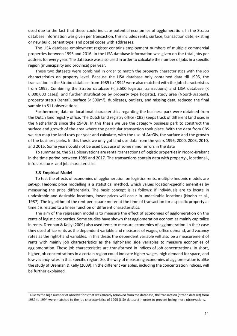
- Ellison-Glaeser Index

The other index used in this thesis is the Ellison and Glaeser’s index (EGI). Ellison and Glaeser (1997)

presented an index for agglomeration economies based on a test of comparison between the observed

geographic distribution of firms and a random distribution. The randomness of a geographic

distribution is in this index defined as the distribution which is expected when there is an absence of

economies of agglomeration. Ellison and Glaeser started with a simple location model where they

16

hypothesize that plants gather together either to internalize externalities from other establishments

or to benefit from local natural advantages. They first defined an index of raw geographic

concentration:

𝐺𝑖 = ∑(𝑠𝑖𝑐 − 𝑥𝑐)2

𝑖

Where sic is the share of industry i’s employment in area c and xc is the share of aggregate logistics

employment in area c. Industrial concentration of an industry i is measured using the Herfindahl-

Hirschman index:

𝐻𝑖 = ∑ 𝑧𝑖𝑗2

𝑗

The Herfindahl-Hirschman index is defined as the sum of squared employment shares by industry

i, where in this case j = 1, 2, …, n, number of firms. The Hi is the function of the number and size

distributions of establishments/firms in industry i. When a region has a small number of establishments

and an uneven size distribution in a certain industry then this index will generally be very high (Ellison

& Glaeser, 1997).

The raw geographic concentration Gi of an industry i should be proportional to its industrial

concentration Hi if there are no agglomeration economies. Ellison and Glaeser show that:

𝐸(𝐺𝑖) = (1 − ∑ 𝑥𝑖2

𝑖

) [𝐻𝑖 + 𝑦(1 − 𝐻𝑖)]

From which they derived an estimator of excess concentration, called the agglomeration index.

ŷ𝑖 =𝐺𝑖 − (1 − ∑ 𝑥𝑖

2𝑖 ) 𝐻𝑖

(1 − ∑ 𝑥𝑖2

𝑖 ) (1 − 𝐻𝑖)

While the Ellison and Glaeser index is somewhat more complex compared to the Location

Quotient, the index is based on standard concentration ratios and can be constructed with readily

available data. The index defines concentration as agglomeration above and beyond what we would

observe if establishments/firms simply chose locations randomly (Ellison & Glaeser, 1997).

The index is very useful in showing if and where there is an excess-concentration of an industry

but does not tell us what the origin of this excess-concentration is, for example natural advantages or

economies of agglomeration. Ellison and Glaeser show that yi is zero when there are no economies of

agglomeration or other natural advantages. Positive values of the index indicating localization of firms

beyond that expected by pure randomness. Whereas negative values show or indicating that

establishment or firms choose to locate more separate or diffusely than expected by randomness.

3.4.5 Fixed effects

In order to account for changes and correlations within the time period of the transactions in the

database (1989-2017), year fixed effects are introduced in the model. Locational fixed effects (COROP

region) are added to control for differences in transaction prices between the various COROP-regions

where the properties are located. A smaller scale is due to the scale of the study area not feasible,

which will also make the results biased.

3.5 Variables description

In table 3.1 detailed information is shown of the employed variables, the variable type (dummy,

categorical, or continuous), the transformation that has been undertaken (some irrelevant data entries

17

were dropped, or the natural logarithm was used for a better fit in the model) and the description of

the variable.

Table 3.1: Description of the variables.

Variable Variable type Transformation Description

Dependent variable

Log Rent per square meter Continuous Natural logarithm Rents per square meter < 15,-

& > 80,- were dropped

Independent variables Property characteristics Log Surface Logistics Continuous Natural logarithm Natural logarithm of the

property logistics surface; Log Surface Office Continuous Natural logarithm Natural logarithm of the

property office surface

Year Build Continuous

The year the property was build

New Property Dummy Dummy for new/existing

build (New = 1) Function Categorical The function of the property;

(1) Manufacturing; (2) Warehouse; (3) Distribution Centre

Locational characteristics Log Surface business park Continuous Natural logarithm Natural logarithm of the

surface of the business park Growth business park Continuous The growth of the surface of

the business park compared to the former land use dataset

Functional urban area Categorical Small FUA combined

with commuting zone, due to low number of observations

Identification of the OECD of urban / rural areas; (1) Small FUA; (2) Medium FUA; (3) Metropolitan FUA; (4) Large Metropolitan FUA

Infrastructural characteristics Highway entrance Continuous Distance to the nearest

highway entrance Train station Continuous Distance to the nearest train

station Traffic Congestion Continuous The length of a congestion

times the duration per quarter a year

Job characteristics Location Quotient Continuous Statistical measure of

concentration based on job figures/data

Ellison-Glaeser index Continuous

COROP fixed effects Categorical COROP region Year fixed effects Categorical Year 1986 & 1988

were dropped Transaction year

18

In table 3.2 the descriptive statistics of the variables of the full sample are shown. These are the

statistics of the variables which are included in the regression analysis. Some of these descriptive

statistics are important to point out. First, regarding the dependent variable rents per square meter,

the mean rent is circa € 40 per square meter, with surfaces averaged of 1,900 m² for logistics and 100

m² for the office space. The maximum price per square meter is almost € 80 per square meter. This

could indicate that this property contains more office space and is basically used as an office. This is

also the reason why observations with higher prices per square meter were dropped from the

database. Also, the share of new properties in the database is only 2.9%, with construction years

running from 1901 to 2014.

Table 3.2: Description statistics of the sample

Variable Obs. Mean Std. Dev. Min Max

Dependent variable

Rent per m² 511 39.98 12.92 15.43 78.41

Independent variables

Property characteristics

Logistics Surface (m²) 511 1,900.67 1,988.30 200 12,676

Office Surface (m²) 511 107,58 193.53 0 1,420

New Property 511 0.029 0.17 0 1

Manufacturing 511 0.22 0.42 0 1

Warehouse 511 0.16 0.37 0 1

Distribution Centre 511 0.62 0.49 0 1

Locational characteristics

Surface business park (ha) 511 329.64 237.39 7.98 856.58

Growth business park (%) 511 20.78 70.98 -89.27 488.61

Commuting Zone/Small FUA 511 0.11 0.31 0 1

Medium FUA 511 0.12 0.32 0 1

Metropolitan FUA 511 0.76 0.43 0 1

Large Metropolitan FUA 511 0.02 0.12 0 1

Infrastructural characteristics

Highway entrance (m) 511 1,951.00 1,758.16 12.00 14,371.60

Train station (m) 511 4,399.37 3,546.90 66.30 16,478.20

Traffic Congestion 511 11.29 1.97 7.70 15.60

Job characteristics

Location Quotient 511 1.33 1.82 0.035 30.63

Ellison-Glaeser index 511 0.67 4.86 -18.17 90.13

Next, approximately 11% of the transactions took place in a small FUA, 12% in a medium FUA, 76%

in a metropolitan area and only 2% in a large metropolitan area. The low number of transactions in a

large metropolitan area can be explained by the fact that only a small area in the province is defined

as a large metropolitan area, this due to the fact of higher population density in the cities of Dordrecht

and Rotterdam, which both aren’t in the study area Noord-Brabant. Lastly, the economies of

agglomeration indices show highly different values indicating municipalities which show high and low

concentrations of logistics activity.

19

4. Results

In this chapter, the results of the hedonic price models are presented which will give an answer to the

three hypotheses mentioned in chapter 2. These will help to answer the main research question: “To

what extent does spatially clustering of logistics firms create economies of agglomeration in the

province of Noord-Brabant?” Multiple hedonic models are set up, with in every subsequent model

extra variables are added. In this way, the impact per addition of characteristics on the property rents

can be measured.

Table 4.1: Baseline specification, models 1, 2 and 3.

Models (1) (2) (3)

Variables (Log Rents per Sqm) (Log Rents per Sqm) (Log Rents per Sqm)

Property characteristics Log Surface Logistics -0.121*** -0.120*** -0.135***

(0.0174) (0.0176) (0.0162)

Log Surface Office 0.0279*** 0.0274*** 0.0148***

(0.00575) (0.00579) (0.00543)

Year Build 0.00754*** 0.00744*** 0.00482***

(0.000782) (0.000789) (0.000771)

New Property 0.105 0.101 0.262***

(0.0734) (0.0737) (0.0698)

Function

Manufacturing -0.00919 -0.00957 -0.0252

(0.0306) (0.0307) (0.0282)

Warehouse -0.0195 -0.0232 -0.0104

(0.0353) (0.0356) (0.0327)

Locational characteristics

Log Surface business park 0.00633 0.00742 0.0116

(0.0120) (0.0122) (0.0114)

Growth business park -0.000064 -0.0000308 0.000176

(0.000210) (0.000189) (0.000180)

Functional urban area

Small FUA -0.128*** -0.122*** -0.153***

(0.0414) (0.0443) (0.0406)

Medium FUA -0.172*** -0.173*** -0.198***

(0.0389) (0.0424) (0.0396)

Large Metropolitan FUA 0.0348 0.346 -0.00521

(0.103) (0.106) (0.106)

COROP Fixed Effects No Yes Yes

Year Fixed Effects No No Yes

Constant -10.582*** -10.406*** -5.385***

(1.557) (1.570) (1.522)

Observations 511 511 511

R-Squared 0.3148 0.3163 0.4825

Standard errors in parentheses ***p<0.01 **p<0.05 *p<0.1

Note: the reference group for New Property is ‘Existing build’; for Function it is ‘Distribution centre’; for Functional urban

area it is ‘Metropolitan FUA’; the coefficients of the variables COROP Fixed Effects and Year Fixed Effects can be found in the

appendix.

20

Table 4.1 presents the results of the first hedonic models. In these models the property and

locational characteristics are added, with in addition the year- and COROP fixed effects. The models

differ whether the fixed effects are added. In these models we can examine the impact of the property

characteristics, locational characteristics, and year/COROP fixed effects on the explained variance (R-

squared).

Before the hedonic models are set up, several assumptions2 are checked regarding the regression

models. These assumptions must be met in order to get non-biased results. The data from the Strabo-

and LISA database are adjusted where necessary.

In model 1 only the control variables for property and location are added. In models 2 and 3, the

year- and COROP fixed effects are added. The R-squared for model 1 and 2 are relatively low

(respectively 31.48% & 31.63%). When adding the year fixed dummies, the R-squared raises to 0.4825

(model 3). Meaning that the variation of the rents per square meter of logistics properties for

approximately 48.25% is explained by the variables in the regression model. Model 3 is used as the

base model for the upcoming hedonic models, therefore this model will be discussed in further detail.

First, the property characteristics: ‘Surface Logistics’, ’Surface Office’, ‘Year Build’ and ‘New

Property’ are all significantly different from zero on a 99% level, indicating that these characteristics

all significantly impact the rents per square meter and therefore are important parameters for logistics

real estate. Also, the variables ‘Small FUA’ and ‘Medium FUA’ are significantly different from zero on a

99% level. Indicating that logistics real estate located in different functional urban areas impacts rents.

Zooming in per variable, we see a coefficient of -0.135 for the variable ‘Surface Logistics’. Because

the dependent variable and the independent variable ‘Surface Logistics’ are transformed to a natural

logarithm, we can interpret the result as follows: if the property surface increases by ten percent, the

rents per square meter decreases by 1.35%. Concluding, properties with larger logistics space show

significantly lower property rents per square meter. Due to a usually higher demand for smaller

logistics units this result is quite understandable. The coefficient of ‘Surface Office’ is 0.0148,

concluding that an increase of office space by ten percent results in an increase of rents by 0.148%.

Regarding new or existing build, new build properties have rents that are approximately 30%3 higher

than existing build properties. Lastly, if the building year increases by one the rents per square meter

will increase by 0.48%. Indicating that newer properties show higher rents per square meter.

Regarding the locational characteristics, we see no significant change in the rents per square meter

influenced by the surface or growth of the business park. The predefined functional urban areas ‘Small

FUA’ and ‘Medium FUA’ are significantly different from zero on a 99% level. In this case due to the fact

the variable type is categorical the Small, Medium and Large Metropolitan FUA’s are compared to the

reference group ‘Metropolitan FUA. This reference group was chosen due to the large number of

transactions which took place in this FUA in the database. First, the variable type ‘Large Metropolitan

FUA’ is not significant significantly different from zero, meaning that the rents per square meter aren’t

different to the rents per square meter in the ‘Metropolitan FUA’. The Small FUA and Medium FUA are

significantly different from zero on a 99% level. The rents per square meter of logistics properties are

14.19% lower in the ‘Small FUA’ and 17.96% lower in the ‘Medium FUA’ compared to the ‘Metropolitan

FUA’. The total results of model 3 are presented in appendix III.

2 The assumptions indicate that, first there is a linear relationship between the dependent and independent variables collectively, this is checked by plotting multiple scatterplots. Second, the homoscedasticity is checked by plotting the studentized residuals (r), observations are dropped when r > 2.5 and r < -2.5. Third, the multicollinearity of the variables is checked with a correlation matrix and later on with VIF values. The VIF values of the variables are all beneath 2.16 which indicate an absence of multicollinearity between the variables. After that heteroscedasticity was checked with the Breusch-Pagan test, which showed no signs of heteroscedastic residuals. Then, the distribution of the residuals was checked with a PP Plot and QQ Plot, and a Skewness/Kurtosis test. Last, significant outliers were identified and dropped using a boxplot.

3 (((exp^ 0.262)-1) *100); (the other results are calculated the same way).

21

Table 4.2 present models 4, 5, 6 and 7, model 3 will serve as the base model. In these models the

infrastructural characteristics are added. In model 7 all variables are added. In model 4, 5 and 6 the

infrastructural characteristics are separately added, which shows the impact per infrastructural

characteristic on the whole model.

Table 4.2: Models 4-7; Base model 3 including infrastructural characteristics.

Models (4) (5) (6) (7)

Variables (Log Rents per

Sqm) (Log Rents per

Sqm) (Log Rents per

Sqm) (Log Rents per

Sqm)

Property characteristic

Log Surface Logistics -0.167*** -0.119*** -0.163* -0.186*

(0.0230) (0.0253) (0.0872) (0.0885)

Infrastructural characteristics

Highway entrance -0.128** -0.118*

(0.0633) (0.0633) Highway entr.* Log Surface Logistics 0.0162* 0.0149*

(0.00867) (0.00866)

Train Station 0.0246 0.0200

(0.0328) (0.0329) Train Station* Log Surface Logistics -0.00389 -0.00337

(0.00454) (0.00456)

Traffic Congestion 0.0715 0.0650

(0.0650) (0.0656) Traffic Cong.* Log Surface Logistics 0.00239 0.00314

(0.00735) (0.00741)

Property characteristics Yes Yes Yes Yes

Locational characteristics Yes Yes Yes Yes

COROP Fixed Effects Yes Yes Yes Yes

Year Fixed Effects Yes Yes Yes Yes

Constant -4.711*** -5.613*** -5.922*** -5.462***

(1.544) (1.536) (1.652) (1.555)

Observations 511 511 511 511

R-Squared 0.4887 0.4839 0.4892 0.4966

Note: Dependent variable is ln (Rents per square meter). Standard errors in parentheses

***p<0.01 **p<0.05 *p<0.1 Note: the coefficients of the variables COROP Fixed Effects and Year Fixed Effects can be found in the appendix.

These infrastructural characteristics were added due to their importance highlighted by different

authors. According to Bok (2009) and Berechman (1994), the logistics real estate sector and their

operations, are all driven by accessibility and the general infrastructure nearby. For foreign logistics

firms, one of the most important determinants, considering location strategy, is the transportation

accessibility (Hong, 2007).

In order to measure the accessibility and infrastructural characteristics on logistics firms and their

real estate, three variables are added to the models. These are the distance to a highway entrance,

22

the distance to a train station and the traffic congestion. In addition to the basic variables, interaction

variables are added. The infrastructural characteristics are interacting with the variable ‘log surface

logistics’. These interaction variables measure the impact of the infrastructure on the property rents,

regarding their logistics surface. Different studies suggest that some firms, based on their size, may

have greater benefits than others regarding economies of agglomeration. According to Shaver & Flyer

(2000) firms which already possess superior technologies and human capital, in this case the larger

firms, do not have the incentive to cluster. On the contrary, Alcácer & Chung (2007) suggest that

smaller firms cannot absorb the spillovers of economies of agglomeration due to their lack of

technology and (human) capital.

When reviewing models 4-7, the variables ‘Highway entrance’ and the interaction variable

‘Highway entrance * Log Surface Logistics’ are the only two variables significantly different from zero.

Concluding, the distance to a train station and the level of congestions and their interactions with the

logistics surfaces do not impact the rents per square meter of logistics real estate. The variable highway

entrance is significant and got a coefficient of -0.118. Meaning that when the distance to the nearest

highway entrance increases by one kilometre the rents per square meter will rise by 11.13%.

Interpreting the interaction variable is somewhat more difficult. In order to measure the impact of

the distance of the highway entrance regarding the logistics surfaces, the coefficients of the variables

in model 7 are put in to the next formula: Coefficient Highway = -0.181 + 0.0149 * Log Surface. Different

surfaces of the logistics space will be filled in, in order to conduct the coefficients. These coefficients

can later on be interpreted as the percentage change of the rents when the distance to the highway

entrance increases by one kilometre. In table 4.3 the logistics surfaces are shown with corresponding

coefficient and percentage change of the rent per square meter.

Table 4.3: Interpretation interaction variable ‘Highway * Log Surface Logistics’

Notable is the difference in percentages regarding the 11.13% calculated above. This can be

explained by the significant impact of the logistics surface on the importance of the distance to the

highway entrance. According to table 4.3, above 2,500 m² logistics surface the rents increases when

the distance to the highway increases. Recalling: “if firms are paying higher rents in a particular location

all else equal, then the location must have some compensating productivity differential (Rosenthal &

Strange, 2005).“ In other words, for the relatively smaller logistics firms the rents are higher closer to

the highway entrance, for the larger firms it’s the other way around. Concluding that the distance to

the highway entrance is a compensating productivity differential for smaller firms, and therefore an

important determinant considering location strategy. This isn’t the case for larger firms.

Table 4.4 presents models 8-11, model 7 will serve here as the base model. In these models the

job concentration variables ‘Location Quotient’ and ‘Ellison-Glaeser index’ are added. Just as in the

previous models, interaction variables are added in order to account for differences in logistics space.

Because of multicollinearity the indices couldn’t be added to the same model. The job concentration

variables are measured and based on the job figures in their respective year. For example, the year the

transaction took place is the same year the job figures are from.

Surface Logistics (m²) 500 1000 1500 2000 2500 5000 10000 15000

Coefficient Highway -0,0254 -0,0151 -0,00903 -0,00475 -0.00142 0,00891 0,0192 0,0253

∆% Rent/m² -2,51% -1,50% -0,90% -0,47% -0.14% 0,89% 1,94% 2,56%

23

Table 4.4: Models 8-11; Base model 7 including job concentration variables.

Models (8) (9) (10) (11)

Variables (Log Rents per

Sqm) (Log Rents per

Sqm) (Log Rents per

Sqm) (Log Rents per

Sqm)

Location Quotient -0.000502 -0.119

(0.00676) (0.148)

LQ* Log Surface Logistic -0.0172

(0.0214)

Ellison-Glaeser index 0.00363* 0.0341

(0.00239) (0.0361)

EGI* Log Surface Logistic -0.00461

(0.00546)

Infrastructural characteristics

Yes Yes Yes Yes

Property characteristics Yes Yes Yes Yes

Locational characteristics

Yes Yes Yes Yes

COROP Fixed Effects Yes Yes Yes Yes

Year Fixed Effects Yes Yes Yes Yes

Constant -5.452*** -5.202*** -5.512*** -5.567***

(1.690) (1.719) (1.618) (1.683)

Observations 511 511 511 511

R-Squared 0.4966 0.4925 0.4991 0.4999

Note: Dependent variable is ln (Rents per square meter). Standard errors in parentheses

***p<0.01 **p<0.05 *p<0.1

In the models 8-11 the only variable that’s significantly different from zero is the ‘Ellison-Glaeser

index’ in model 10. The variable is significantly different from zero on a 90% level. This significance

level indicates lower reliability of the estimates and therefore uncertainty in the results. Nevertheless,

the concentration index significantly effects the logistics property rents. The coefficient of the variable

is positive at 0.00363. Recalling the interpretation of the Ellison-Glaeser index: ‘when the index is zero

there are no economies of agglomeration there are no economies of agglomeration or other natural

advantages. Positive values of the index indicate localization of firms beyond that expected by pure

randomness. Whereas negative values show or indicate that establishments or firms choose to locate

more separate or diffusely than expected by randomness.’ Concluding this interpretation, the positive

value indicates localization of firms beyond that expected by pure randomness. Firms will locate to

places where logistics jobs are concentrated. Whereas rents rise with 0.36% when the Ellison-Glaeser

index increases by one point. Respectively, when the index raises by ten points, the rents per square

meter increases by 3.6%.

Second, the interaction variables are not significant in the models, meaning that we cannot accept

hypotheses 3. Company size only effects, based on the previous models, the importance of a nearby

highway ramp and has no impact on the benefits of economies of agglomeration. Therefore, we

contradict the findings of Shaver & Flyer (2000) and Alcácer & Chung (2007), which all argued that

company size does impact the benefits of economies of agglomeration.

24

5. Discussion

5.1 Company size and economies of agglomeration

Due to the increasingly clustering of logistics activities, many researchers have tried to examine

and measure the attribution of economies of agglomeration on this clustering. Marshall (1920) was

the first who described three main sources of economies of agglomeration, namely labour market

pooling, input sharing, and knowledge spillovers. Same industry firms which were clustered in a specific

area or region should all benefit from these main sources of economies of agglomeration. According

to Shaver & Flyer (2000) and Alcácer & Chung (2007) this equally benefitting isn’t the case. They stated

that firms which already possesses superior technologies, suppliers, distributors, and human capital

does not have the incentive to cluster with other same industry firms. Also, whether a firm can absorb

the economies of agglomeration is crucial when clustered. Some smaller firms can’t leverage the

economies due to a lack in (human) capital.

In this study, the effects of company size on economies of agglomerations have been plotted in

the hedonic models. Starting with interaction models regarding infrastructural characteristics. Many

authors highlighted the importance of the general infrastructure and accessibility as the main factor

for logistics clusters (Bok, 2009; Berechman, 1994; Hong, 2007). These studies didn’t account for

differences in company size regarding the importance of infrastructure. According to the hedonic

models in this study, smaller logistics firms do have an incentive to locate near a highway entrance. In

contrast to the bigger firms, which show higher property rents further away from highway entrances.

Concluding, the distance to the highway can be seen as a compensating productivity differential for

smaller firms, and therefore an important determinant considering location strategy. A possible

explanation for this could be the fact that larger firms more or mostly depend on their human capital

and superior technology and knowledge in contrast to their location near infrastructural nodes.

When measuring the effects of company size on the property rents, regarding the concentration

of logistics jobs, no significant effects can be found in the hedonic models. Concluding that there is no

difference in the importance of the concentration of logistics jobs nearby, regarding the company size.

5.2 Concentration of jobs and economies of agglomeration

All over the world, new logistics clusters are in development or existing clusters are expanding.

Many studies suggest this is mainly due to the presence of economies of agglomeration (Rivera et al.,

2014). Economies of agglomeration are an economy of scale and can occur when economic activity is

spatially clustered (Mukkala, 2004). Regarding the logistics sector, these economies of agglomeration,

can provide firms with a more flexible labour market, combining of transport flows, a decrease in

distance between customers, and clustered firms can put in more weight in lobbying for improved

infrastructure and regulatory relief with the local government (Van Donselaar et al., 1999; Van den

Heuvel et al., 2012; Rivera et al., 2014).

Within the existing literature there is an array of research on economies of agglomeration. Many

findings suggest that these economies impacts the rents by up to five percent, albeit in the office sector

(Drennan & Kelly, 2009; Koster et al., 2014). Other studies argued the downside of clustering of similar

firms. Agglomeration diseconomies can occur, such as high land/lease prices or an increase in

competition (Van den Heuvel, 2013; Holmes & Stevens, 2002).

In this study job concentration indices were used in order to measure economies of agglomeration

in the logistics sector. These indices both measured the concentration of logistics jobs in a specific

municipality. Only one of the two indices had a significant impact on the rents of logistics properties.

This concentration index is significantly different from zero on a 90% significance level, meaning that

the reliability of the results is lower compared to when significant on a 95% or 99% significance level.

Concluding that, regarding the logistics sector, there is evidence of economies of agglomeration

25

benefitting firms that cluster, but that these results can be described as less reliable. Also, the Location-

Quotient index was not significantly different from zero on all significance levels indicating no impact

of clustered jobs on the property rents.

5.3 Data limitations and further research

Just like other studies, this research has its limitations concerning the data. First of all, we used the

rents as a measurement for economies of agglomeration. Very few studies use rents in order to

measure the presence of agglomeration economies. Still some have shown that agglomeration

economies mainly capitalize in rents (Koster et al., 2014; Arzaghi & Henderson, 2008; Drennan & Kelly,

2009). Suggested is to use property yields in order to measure economies of agglomeration. The

property yield is calculated by dividing the annual rental income on the costs of buying it. Therefore,

the property yields are susceptible to the market conditions, where higher yields reflect higher risks

for potential investors. In other words, when the demand for property is high, the cost of buying will

increase, which then automatically lowers the yield. Rents do not explicitly reflects demand, because

higher rents can easily be the result of other property- or locational characteristics. Second, the

database of Strabo contained of thousands of transactions. Unfortunately, due to missing or lacking

data, and further stratification the database was largely reduced to only 511 observations. A larger

database would result in more accurate findings. Last, the LISA dataset contains data of jobs from 1995

to 2016. Because of the high number of observations that was already removed from the database,

the transactions (Strabo dataset) from 1989 to 1994 were matched to the job characteristics of 1995

(LISA dataset) in order to prevent losing more observations.

For further research on economies of agglomeration in the logistics sector it is suggested to

research this phenomenon on a smaller regional scale. The database must be sufficient when studying

a smaller region. Thereby, a combination of quantitative and qualitative research could and should

give a broader perspective on the matter. It is very interesting to know why individual logistics firms

chose a specific location to settle. And if this is in a specific cluster, what benefits or disbenefits they

experience from it.

6. Conclusion

This paper investigated the effect of economies of agglomeration on the rents of logistics real

estate. The approach to use rents stems from the quality-of-life literature and means: “if firms are

paying higher rents in a particular location all else equal, then the location must have some

compensating productivity differential (Rosenthal & Strange, 2005).“ Rents of logistics properties

should be higher when co-locating with same industry firms due to different advantages such as an

increased productivity, easier access to information, ease of new business formation, new

technological and delivery possibilities, and benefits rooted in working together with other institutions

such as universities and public organizations (Rivera et al., 2016; Porter, 1998).

To estimate the effect, multiple hedonic pricing models were conducted. Hence, giving an answer on

the main question: “To what extent does spatially clustering of logistics firms create economies of

agglomeration in the province of Noord-Brabant?”

The findings did not all support the three hypotheses mentioned in chapter 2.2. First, logistics firms

only pay significant higher property rents when located near a highway ramp, regarding properties

with logistics space less than 2,500 m². This is not the case for firms bigger than 2,500 m². Second,

logistics firms pay higher prices in predefined Urban areas. The rents per square meter of logistics

properties are 14.19% lower in the ‘Small FUA’ and 17.96% lower in the ‘Medium FUA’ compared to

the ‘Metropolitan FUA’. These functional urban areas are based on population numbers, which

indicate that near higher sources of population, the rents are significantly higher. Lastly, with the use

of the LISA database and the Herfindahl-Hirschman index the concentration indices like the Ellison-

26

Glaeser index and Location Quotient were constructed. While the Ellison-Glaeser index is somewhat

more complex compared to the Location Quotient, both indices are based on standard concentration

ratios and can be constructed with readily available data. Of these concentrations indices the Ellison-

Glaeser index has a significant effect on the rents of logistics real estate. Recalling the interpretation

of the Ellison-Glaeser index: ‘when the index is zero there are no economies of agglomeration or other

natural advantages. Positive values of the index indicating localization of firms beyond that expected

by pure randomness. Whereas negative values show or indicating that establishment or firms choose

to locate more separate or diffusely than expected by randomness.’ When the Ellison-Glaeser index

rises by ten points the rents per square meter grow by 3.6%, indicating that in regions where

localization of firms are beyond that expected by pure randomness, the rents increase. Carefulness is

required however. Because the significance is based on a 90% level, the impact can be considered less

reliable than to be preferred. Also, the Location-Quotient was not significantly different from zero on

all significance levels indicating no impact of clustered jobs on the property rents.

27

References

Arzaghi, M. & Henderson, J.V. (2008). Networking off Madison Avenue. Review of Economic Studies,

75, 1011-1038.

Berechman, J. (1994). Urban and regional economic impacts of transportation investment: a critical

assessment and proposed methodology. Transport. Res. Part A: Policy Pract. 28(4), 351-362.

Bok, M. (2009). Estimation and validation of a microscopic model for spatial economic effects of

transport infrastructure. Transport. Res. Part A: Policy Pract. 43, 44-59.

Bounie, N. & Blanquart, C. (2017). Logistics Centers and Agglomeration Economies: Logistics Clusters

or Co-located Logistics Activities? The French Case. World Conference on Transport Research.

Cairncross, F. (1997). The Death of Distance. Orion Business Books, London.

Carbonara, N., Giannoccaro, I. & Pontrandolfo, P. (2002). Supply chains within industrial districts: A

theoretical framework. International Journal of Production Economics, Vol. 76, Issue 2, pp. 159-176.

Carlton, D.W. (1983). The Location and Employment Choices of New Firms: An Econometric Model

with Discrete and Continuous Endogenous Variables. Review of Economics and Statistics, 65: 440-449.

Catin, M. (1997). Disparités spatiales de productivité, accumulation du capital et économies

d’agglomération. Revue économique, Vol. 48, No. 3, pp. 579-589.

Chatterjee, S. (2003). Agglomeration Economies: The Spark That Ignites a City? Business Review, 6(Q4),

pp. 6-13.

Council of the Americas, 2011. Join us for Panama: Where the World Meets. Council of the Americas.

Courlet, C. (2008). L’économie territorial, Presses Universitaires de Grenoble, Grenoble.

Cruijssen, F., Cools, M. & Dullaert, W. (2007a). Horizontal cooperation in logistics: opportunities and

impediments. Transportation Research Part E 43, 129-142.

Cruijssen, F., Dullaert, W. & Fleuren, H. (2007b). Horizontal cooperation in transport and logistics: a

literature overview. Transportation Journal 46, 22-39.

Delgado, M. Porter, M. & Stern, S. (2010). Clusters and entrepreneurship. J. Econ. Geogr. 10, 495-518.

Dell’Orco, M., Sassanelli, D. & Tiso, A. (2009). Optimization of logistics in industrial districts through

creation of a community agents. Chemical Engineering Transactions, Vol. 18, pp. 321-326.

Drennan, M.P. & Kelly, H.F. (2009). Measuring urban agglomeration economies with office rents.

Journal of Economic Geography, 11 (2011) pp. 481-507.

Ellison & Glaeser (1997). Geographic concentration in U.S. manufacturing industries: A dartboard

approach, NBER working paper no. 4840.

28

Emsi (2011). Understanding Location Quotient. [online] Available at:

https://www.economicmodeling.com/2011/10/14/understanding-location-quotient-2/ [Accessed 15-

09-2019].

Feitelson, E. & Salomon, I. (2000). The implication of differential network flexibility for spatial

structures. Transport. Res. Part A: Policy Pract. 34, 459-479.

Fujita, M. & Krugman, P. (2004). The new economic geography: past, present and the future. Papers

in Regional Science, 83, 139-164.

Holmes. T.J. & Stevens, J.J. (2002). Geographic concentration and establishments scale. The Review of

Economics and Statistics 84, 682-692.

Government of Panama, 2010. Panama Plan Estrategico de Gobierno 2010-2014. Gaceta Oficial Digital.

Henderson, J.V. (1986). Efficiency of resource usage and city size. Journal of Urban Economics, 19, 47-

70.

Henderson, J.V. (2003). Marshall’s scale economies. J. Urban Econ. 53(1), 1-28.

Henderson, J.V. & Shalizi, Z. (2001). Geography and development. J. Urban Econ. 53(1), 1-28.

Hoehn, J.P., Berger, M.C. & Blomquist, G.C. (1987). A hedonic model of interregional wages, rents,

and amenity values. Journal of regional science, vol. 27, no. 4.

Hong, J. (2007). Transport and the location of foreign logistics firms: the Chinese experience. Transport.

Res. Part A: Policy Pract, 41, 597-609.

Hoover, E. (1937). Localization Theory and the Shoe and the Leather Industries. Harvard University

Press, Cambridge.

Industrial (2018). Logistics real estate: Dutch Market Report 2018. [online] Available at:

https://www.industrial.nl/wp-content/uploads/2018/02/Report-LOGISTICS-REAL-ESTATE_Dutch-

Market-Report-2018-2.pdf [Accessed 12-02-2019].

Isserman, A.M. (1997). The location quotient approach to estimating regional economic impacts.

Journal of the American Institute of Planners.

Jara-Díaz, S.R. & Basso, L.J. (2003). Transport cost functions, network expansion and economies of

scope. Transportation Research Part E 39, 271-288.

Kasarda, J. (2008). The Evolution of Airport Cities and the Aerotropolis. Airport Cities: The Evolution.

Insight Media, London.

Koster, H.R.A., Van Ommeren, J. & Rietveld, P. (2014). Agglomeration Economies and Productivity: A

Structural Estimation Approach Using Commercial Rents. Economica, Vol. 81, no. 321.

29

Lasserre, F. (2008). Logistics and the Internet: transportation and location issues are crucial in the

logistics chain. Journal of Transport Geography 12, 73-84.

Logistiek (2019). Logistieke hotspots van 2019. [online] Available at: https://intern.logistiek.nl/poster-

logistieke-hotspots-2019?_ga=2.56487022.430825292.1557310091-1217709000.1534862583

[Accessed 12-5-2019].

Malmberg, A. & Maskell, P. (1997). Towards an explanation of regional specialization and industry

agglomeration. European Planning Studies 5, 25-41.

Marshall, A. (1920). Principles of Economics (London: MacMillan).

Masson, S. & Petiot, R. (2014). Dynamiques spatiales des activités logistiques d’entreposage et

économies d’agglomération: une analyse économétrique. 51st Colloque ASRDLF, Marne-la-Vallée.

Mattarocci, G. & Pekdemir, D. (2017). Logistic Real Estate Investment and REITs in Europe.

Moomaw, R.L. (1981). Productivity and city size: a critique of the evidence. Quarterly Journal of

Economics, 96, 675-688.

Mukkala, K. (2004). Agglomeration Economies in the Finnish Manufacturing Sector. Applied Economics,

36, 2149-2427.

Peiser, R. B. & Schwanke, D. (1992). Professional Real Estate Development, Urban Land Institute.

Washington: Dearborn Financial Publishing Inc.

Porter, M. (1998). Clusters and the new economics of competitiveness. Harv. Bus. Rev. 76, 77-90.

Porter, M. (2000). Location, competition, and economic development: local clusters in a global

economy. Econ. Develop. Quart. 12, 15-42.

Rietveld, P. (1994). Spatial economic impacts of transport infrastructure supply. Transport. Res. Part

A: Policy Pract. 28(4), 329-341.

Rivera, L. (2014). Logistics Clusters: Prevalence and Impact. MIT, pp. 129.

Rivera, L., Sheffi, Y. & Knoppen, D. (2016). Logistics clusters: The impact of further agglomeration,

training and firm size on collaboration and value added services. Int. J. Production Economics, 179, 285-

294.

Rivera, L., Sheffi, Y. & Welsch, R. (2014). Logistics agglomeration in the US. Transportation Research

Part A 59, 222-238.

Rosenthal, S.S. & Strange, W.C. (2002). Evidence of the Nature and Sources of Agglomeration

Economies. Prepared for the Handbook of Urban And Regional Economies, Volume 4.

Rosenthal, S.S. & Strange, W.C. (2005). The Geography of Entrepreneurship in the New York

Metropolitan Area. Reserve Bank of New York Economic Policy Review, 11, 29-53.

30

Saxenian, (1994). Regional Advantage: Culture and Competition in Silicon Valley and Route 128.

Harvard University Press, Cambridge, MA.

Shaver, M.J. & Flyer, F. (2000). Agglomeration Economies, Firm Heterogeneity, and Foreign Direct

Investment in the United States. Strategic Management Journal, Vol. 21, no. 12, pp. 1175-1193.

Sveikauskas, L. (1975). The productivity of cities. Quarterly Journal of Economics, 89, 393-413.

Van den Heuvel, F.P., De Langen, P.W., Van Donselaar, K.H. & Fransoo, J.C. (2012). Spatial

concentration and location dynamics in logistics: the case of a Dutch province. Beta Working Paper

386, Research School for Operations Management and Logistics.

Van den Heuvel, F.P., De Langen, P.W., Van Donselaar, K.H. & Fransoo, J.C. (2013). Proximity matters:

Synergies through co-location of logistics establishments. International Journal of logistics: Research

and Applications, pp. 19.

Van Donselaar, K. Kokke, K. & Allessie, M. (1999). Performance measurement in the transportation and

distribution sector. International Journal of Physical Distribution & Logistics Management 28, 434-450.

Wouters, M. Kokke, K. Theeuwes, J. & Van Donselaar, K. (1999). Identification of critical operational

performance measures – a research note on a benchmarking study in the transportation and

distribution sector. Management Accounting Research 10, 439-452.

Wu, L. Yue, X. & Sim, T. (2006). Supply clusters: a key to China’s cost advantage. Supp. Chain Manage.

Rev., 46-51.

31

Appendix I: Business parks areas in Noord-Brabant, 2000, 2003, 2010 and 2015.

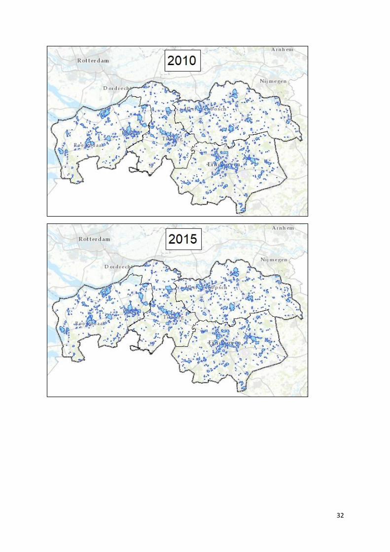
32

33

Appendix II: OLS assumptions

Correlation Matrix

Homoscedasticity

Correlation Matrix

Log Rent per Sqm 1.00

Log Surface Logistics -0.2707 1.00

Log Surface Office 0.2418 0.0409 1.00

Year Build 0.4009 0.0103 0.1626 1.00

New Property 0.0992 0.0036 0.0245 0.0823 1.00

Manufacturing 0.0331 -0.0727 0.0081 0.0281 0.0191 1.00

Warehouse -0.0769 0.2303 -0.0056 0.0161 -0.0451 -0.2346 1.00

Distribution Centre 0.0301 -0.1126 -0.0027 -0.0362 0.0180 -0.6755 -0.5583 1.00

Log Surface business park 0.0173 0.0903 0.0612 0.0554 -0.0219 0.0126 0.0282 -0.0322 1.00

Growth business park 0.0132 -0.0618 0.0347 0.0402 -0.0263 -0.0087 -0.0475 0.0435 0.1662 1.00

Small FUA -0.0913 -0.0127 -0.0012 0.0267 -0.0604 0.0280 0.0354 -0.0507 0.0997 0.2292 1.00

MediumFUA -0.1948 0.0726 -0.0388 -0.0431 -0.0274 -0.0625 -0.0288 0.0752 -0.0357 -0.0659 -0.1267

Metropolitan FUA 0.2027 -0.0804 -0.0012 -0.0071 0.0708 0.0353 -0.0127 -0.0205 -0.0586 -0.1710 -0.6168

Large Metropolitan FUA 0.0352 0.1206 0.1077 0.0696 -0.0219 -0.0292 0.0299 0.0022 0.0455 0.1874 -0.0438

Highway entrance -0.0649 -0.0262 -0.0067 -0.0750 -0.0645 0.0094 0.0263 -0.0280 0.0620 -0.0110 0.0406

Train Station 0.0042 0.0048 0.0023 0.1421 -0.0727 0.0553 0.0231 -0.0648 -0.0068 0.1897 0.6049

Traffic Congestion 0.2666 0.0984 0.0866 0.1976 -0.0423 0.0255 0.0338 -0.0474 0.0559 0.0031 -0.0359

Midden Noord-Brabant -0.0802 -0.0223 -0.0687 -0.1054 -0.0788 0.0221 -0.0865 0.0468 0.1112 0.2336 0.2123

Noordoost Noord-Brabant 0.0060 -0.0754 0.0059 0.0441 0.0254 -0.0516 0.0233 0.0264 -0.1197 -0.0555 0.2117

West Noord-Brabant -0.0988 0.1808 -0.0243 -0.0171 0.0183 -0.0343 0.0268 0.0089 0.0243 -0.0669 -0.1078

Zuidoost Noord-Brabant 0.1531 -0.0905 0.0729 0.0624 0.0233 0.0595 0.0232 -0.0684 -0.0091 -0.0741 -0.2474

Location Quotient -0.0273 -0.0171 -0.0315 -0.0967 -0.0068 0.0436 -0.0336 -0.0117 -0.0573 -0.0208 -0.1474

Ellison-Glaeser index 0.0175 0.0352 0.0802 -0.0225 -0.0494 0.0154 0.0064 -0.0180 0.0515 0.0147 -0.0142

Warehouse Distribution

Centre

Log Surface

business park

Growth

business park

Small FUALog Rent per

Sqm

Log Surface

Logistics

Log Surface

Office

Year Build New Property Manufacturing

Medium FUA 1.00

Metropolitan FUA -0.6478 1.00

Large Metropolitan FUA -0.0460 -0.2240 1.00

Highway entrance 0.0112 -0.0343 -0.0123 1.00

Train Station -0.1701 -0.3159 0.0187 -0.0525 1.00

Traffic Congestion 0.0068 -0.0266 0.1635 0.0102 0.0517 1.00

Midden Noord-Brabant -0.1652 -0.0129 -0.0571 0.2110 0.1069 -0.0599 1.00

Noordoost Noord-Brabant 0.1133 -0.2200 -0.0645 0.0132 -0.0039 -0.0601 -0.2317 1.00

West Noord-Brabant 0.3076 -0.2113 0.1994 -0.1458 0.0180 0.0912 0.2865 -0.3236 1.00

Zuidoost Noord-Brabant -0.2598 0.4011 -0.0898 -0.0399 -0.0989 0.0121 0.3227 -0.3644 -0.4505 1.00

Location Quotient -0.0319 0.1192 0.0404 -0.0051 -0.0365 -0.0479 0.2195 0.0267 0.0330 -0.2291 1.00

Ellison-Glaeser index 0.0754 -0.0552 0.0300 -0.0400 0.0050 -0.0314 0.0407 0.0103 0.0650 -0.0385 0.0079 1.00

Ellison-Glaeser

index

Traffic

Congestion

Midden Noord-

Brabant

Noordoost Noord-

Brabant

West Noord-

Brabant

Zuidoost Noord-

Brabant

Location

Quotient

Medium FUA Metropolitan

FUA

Large

Metropolitan

Highway

entrance

Train Station

-2-1

01

2S

tudentized r

esid

uals

9 10 11 12 13 14Fitted values

34

VIF

Testing normality assumption with residuals

EGI 1.12 0.889058

LQ 1.25 0.800878

Trainstati 1.90 0.527102

Highway 1.14 0.877192

WestNoordB 1.88 0.530883

NoordoostN 1.77 0.563768

MiddenNoor 1.75 0.570542

LargeMetrFUA 1.26 0.796207

MediumFUA 1.38 0.725374

CommutingZ~e 2.16 0.463510

GrowthBBGA~a 1.36 0.734799

LogAreaBBG 1.20 0.831880

Warehouse 1.20 0.834598

Manufactur 1.14 0.878868

New 1.15 0.868538

Bouwjaar 1.29 0.777714

LogSurface~e 1.16 0.859294

LogSurface~c 1.20 0.835377

Variable VIF 1/VIF

ur 511 0.8407 0.0300 4.75 0.0931

Variable Obs Pr(Skewness) Pr(Kurtosis) adj chi2(2) Prob>chi2

joint

Skewness/Kurtosis tests for Normality

ur 511 0.99620 1.303 0.637 0.26215

Variable Obs W V z Prob>z

Shapiro-Wilk W test for normal data

0.0

00

.25

0.5

00

.75

1.0

0N

orm

al F

[(u

r-m

)/s]

0.00 0.25 0.50 0.75 1.00Empirical P[i] = i/(N+1)

-1-.

50

.51

ur

-1 -.5 0 .5 1Inverse Normal

Prob > chi2 = 0.8094

chi2(1) = 0.06

Variables: fitted values of LogRentSqm

Ho: Constant variance

Breusch-Pagan / Cook-Weisberg test for heteroskedasticity

35

Appendix III: Regression result of the base model.

_cons -5.38511 1.522089 -3.54 0.000 -8.376083 -2.394136

2017 .267964 .1901345 1.41 0.159 -.105659 .641587

2016 .3706183 .1036307 3.58 0.000 .1669793 .5742572

2015 .3617198 .087728 4.12 0.000 .1893302 .5341094

2014 .1764327 .0902749 1.95 0.051 -.0009616 .353827

2013 .3153554 .1034557 3.05 0.002 .1120602 .5186505

2012 .3029378 .1033778 2.93 0.004 .0997957 .5060799

2011 .4493997 .0948097 4.74 0.000 .2630944 .6357051

2010 .4479415 .1220132 3.67 0.000 .2081801 .687703

2009 .3739299 .0868363 4.31 0.000 .2032925 .5445673

2008 .3803448 .0837169 4.54 0.000 .2158373 .5448523

2007 .3771729 .0864301 4.36 0.000 .2073338 .5470119

2006 .3791466 .0879159 4.31 0.000 .2063879 .5519053

2005 .3344196 .0835567 4.00 0.000 .1702269 .4986124

2004 .2596913 .0830764 3.13 0.002 .0964425 .4229402

2003 .175531 .0905462 1.94 0.053 -.0023964 .3534584

2002 .4158121 .0836821 4.97 0.000 .251373 .5802513

2001 .3934781 .0854756 4.60 0.000 .2255147 .5614416

2000 .3271426 .0799966 4.09 0.000 .1699456 .4843396

1999 .2736787 .0882691 3.10 0.002 .1002259 .4471315

1998 .1869479 .0830426 2.25 0.025 .0237654 .3501304

1997 .0816853 .0818898 1.00 0.319 -.0792319 .2426025

1996 .1426462 .0855807 1.67 0.096 -.0255237 .3108162

1995 .0616598 .0827646 0.75 0.457 -.1009763 .224296

1994 .167627 .0950056 1.76 0.078 -.0190634 .3543174

1993 -.0567376 .0891018 -0.64 0.525 -.2318268 .1183516

1992 .2022552 .0927192 2.18 0.030 .0200577 .3844526

1991 -.0385608 .0957328 -0.40 0.687 -.2266802 .1495586

1990 -.1104912 .0964824 -1.15 0.253 -.3000836 .0791012

Jaar

WestNoordB -.0220776 .0328068 -0.67 0.501 -.0865445 .0423893

NoordoostN .0425205 .0352017 1.21 0.228 -.0266524 .1116933

MiddenNoor -.0208016 .035918 -0.58 0.563 -.091382 .0497788

LargeMetrFUA -.0052079 .0993071 -0.05 0.958 -.2003509 .1899351

MediumFUA -.1980962 .039562 -5.01 0.000 -.2758374 -.120355

CommutingZone -.1533571 .0406205 -3.78 0.000 -.2331782 -.0735359

GrowthBBGArea .0001763 .0001802 0.98 0.328 -.0001778 .0005305

LogAreaBBG .0115549 .0114054 1.01 0.312 -.0108573 .033967

Warehouse -.0104195 .0326729 -0.32 0.750 -.0746232 .0537842

Manufactur -.0251862 .0282475 -0.89 0.373 -.0806939 .0303215

New .2618086 .0698372 3.75 0.000 .1245753 .399042

Bouwjaar .0048263 .0007709 6.26 0.000 .0033114 .0063412

LogSurfaceOffice .0148284 .0054339 2.73 0.007 .0041505 .0255064

LogSurfaceLogistic -.1353879 .016264 -8.32 0.000 -.1673473 -.1034285

LogRentSqm Coef. Std. Err. t P>|t| [95% Conf. Interval]

Total 56.1864766 510 .110169562 Root MSE = .24927

Adj R-squared = 0.4360

Residual 29.0792568 468 .062135164 R-squared = 0.4825

Model 27.1072198 42 .645409994 Prob > F = 0.0000

F(42, 468) = 10.39

Source SS df MS Number of obs = 511