logistic mixed effects models a glmm for binary data takes the

2009 Jon Wakefield, Stat/Biostat 571

Logistic Mixed Effects Models

A GLMM for binary data takes the binomial exponential family, with canonical

link being logistic.

We have

Stage 1: Yij ∼ind Binomial(nij , pij) with

log

„pij

1 − pij

«= xijβ + zijbi

Stage 2: bi ∼iid N(0, D).

Marginal moments are not available in closed form.

We initially consider the model with a random intercept only, bi ∼ N(0, σ20).

278


Parameter Interpretation

For the random intercepts model the conditional parameters βc and marginal

parameters βm are approximately linked through

E[Y ] =exp(xβm)

1 + exp(xβm)= Eb{E[Y |b]}

= Eb

»exp(xβc + b)

1 + exp(xβc + b)

–≈ exp(xβc/[c2σ2

0 + 1]1/2)

1 + exp(xβc/[c2σ20 + 1]1/2)

where c = 16√

3/(15π). Hence the marginal coefficients are attenuated towards

zero; Figure 21 illustrates for particular values of β0, β1, σ20 .

For the model

log

„E[Y | b]

1 − E[Y | b]

«= xβc + zb

where b ∼iid Nq+1(0, D) we obtain

E[Y ] ≈exp

`xβc | c2DzzT + Iq+1 |−(q+1)/2

´

1 + exp`xβc | c2DzzT + Iq+1 |−(q+1)/2

´

so that

βm ≈| c2DzzT + Iq+1 |−(q+1)/2 βc

279


The above follows from approximating the logistic CDF by that of a normal

CDF. Specifically,

G(x) = (1 + e−x)−1

is the CDF of a logistic random variable and

G(x) ≈ Φ(cx)

where c = 16√

3/(15π) (Johnson and Kotz, 1970).

280


0 1 2 3 4 5

0.00.2

0.40.6

0.8

1.0

x

Prob

abilit

y

Figure 21: Individual-level curves (dotted lines) from random intercepts logistic

GLMM with log(E[Y | b])/(1 − E[Y | b])) = β0 + β1x, with β0 = −2, β1 =

1 and b ∼iid N(0, 22), along with marginal curve (solid curve). Approximate

attenuation is 1.54.

281


Specifying the Parameters of a Wishart Prior

Suppose we have

b|W ∼ Np(0, W)

W ∼ Wishart(r, S)

We derive the marginal distribution for b:

p(b) =

Zp(b|W) × π(W)dW

∝Z

|W |1/2 exp

„−bTWb

2

«|W |(r+p−1)/2 exp

„−1

2tr(WS−1)

«dW

=

Z|W |(r+p+1−1)/2 exp

„−1

2tr(W [bbT + S−1)

«dW

— the integrand is a Wishartp{r + 1, (S−1 + bbT)−1}

282


We know the normalizing constant of a Wishart distribution:

p(b) = |S−1 + bbT|−(r+1)/2

∝ |Ip + SbbT|−(r+1)/2

= (1 + bTSb)−(r+1)/2

which is a Tp{0, [(r − p + 1)S]−1, d = r − p + 1} density.

The margins of a multivariate Student’s t distribution are t and so we can

specify the parameters r and S using the same technique as with the gamma,

Ga(a, b), noting that a = r/2, b = 1/[2S].

283


Non-linear Mixed Effects Models

We now turn to a class of models that are not GLMs — we begin with a

motivating example.

Example: Pharmacokinetics of Theophylline

Twelve subjects given an oral dose of the anti-asthmatic agent theophylline,

with 11 concentration measurements obtained from each individual over 25

hours.

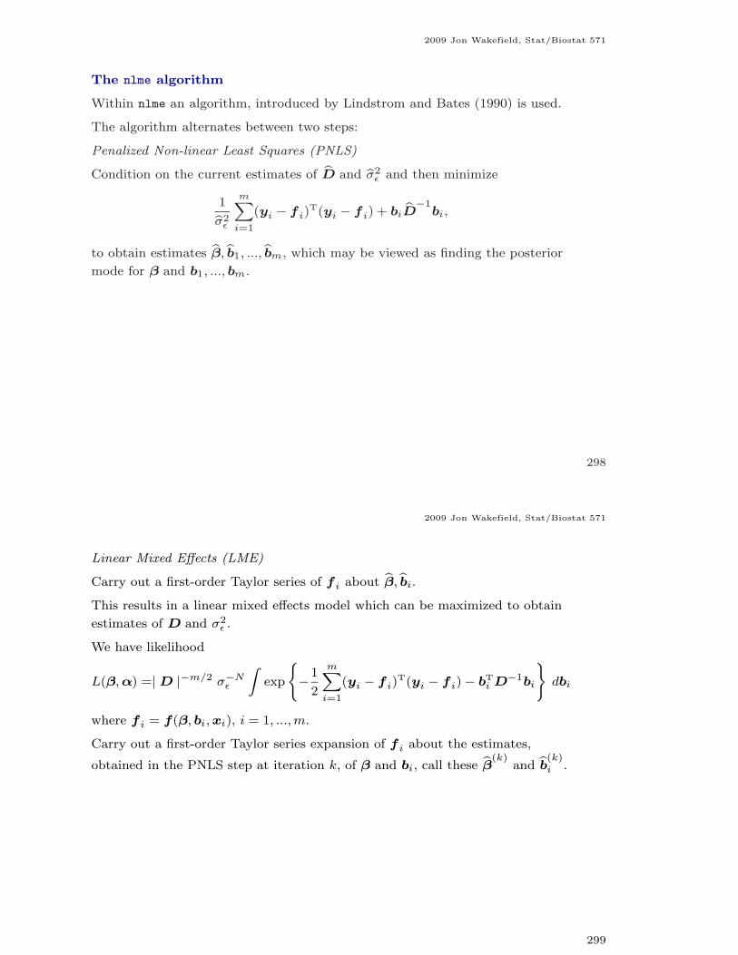
Figure 22 shows the concentration-time data.

The curves follow a similar pattern but there is clearly between-subject

variability. For these data the the one-compartment model with first-order

absorption and elimination is a good starting point for analysis.

The mean concentration at time point t is often modeled as:

f(η, t) =Dkeka

Cl(ka − ke){exp(−ket) − exp(−kat)}

where D is the initial dose.

284


Time since drug administration (hr)

Theo

phyll

ine co

ncen

tratio

n in s

erum

(mg/l

)

0

2

4

6

8

10

0 5 10 15 20 25

6 7

0 5 10 15 20 25

8

11 3

0

2

4

6

8

10

20

2

4

6

8

10

4 9 12

10

0 5 10 15 20 25

1

0

2

4

6

8

10

5

Figure 22: Concentration time data for Theophylline.285


Non-Linear Mixed Effects Model Structure

In a nonlinear mixed model (NLMEM) the first stage of a linear mixed model

is replaced by a nonlinear form. We describe a specific two-stage form that is

useful in many longitudinal situations.

Stage 1: Response model, conditional on random effects, bi:

yi = fij(ηij , tij) + ǫij , (48)

where fij is a nonlinear function and

ηij = xijβ + zijbi,

where

• a (k + 1) × 1 vector of fixed effects, β,

• a (q + 1) × 1 vector of random effects, bi, with q ≤ k.

• xi = (xi1, ..., xini)T, the design matrix for the fixed effect with

xij = (1, xij1, ..., xijk)T, and

• zi = (zi1, ..., zini)T, and design matrix for the random effects with

zij = (1, zij1, ..., zijq)T.

286


Stage 2: Model for random terms:

E[ǫi] = 0, var(ǫi) = Ei(α),

E[bi] = 0, var(bi) = D(α),

cov(bi, ǫi) = 0

where α is the vector of variance-covariance parameters.

A common model assumes

ǫi ∼ind N(0, σ2ǫ Ini

), bi ∼iid N(0, D).

Let α represent σ2ǫ and the parameters of D and N =

Pi ni.

287


Likelihood Inference for the Nonlinear Mixed Effects Model

As with the linear mixed and generalized linear mixed models already

considered the likelihood is defined with respect to fixed effects β and variance

components α:

p(y|β, α) =

mY

i=1

Z

bi

p(yi|bi, β, σ2ǫ ) × p(bi|D) dbi

The first difficulty is how to calculate the required integrals, which for

non-linear models are analytically intractable, recall for linear models they were

available in closed form. For nonlinear models even the first two moments are

not available in closed form in general:

E[Yij | β, α] = Ebi|D [fij(xijβ + zijbi, tij)] 6= f(β,0, xij)

var(Yij | β, α) = σ2ǫ + varbi|D [fij(xijβ + zijbi, tij)]

cov(Yij , Yij′ | β, α) = covbi|D(fij(xijβ + zijbi, tij), fij′(xij′β + zij′bi, tij′)]

cov(Yij , Yi′j′ | β, α) = 0, i 6= i′

The data do not in general have a closed-form marginal distribution.

288


As with the GLMM there are two issues with respect to implementation:

• How do we evaluate the integrals, and

• how do we maximize the resultant likelihood?

As with the LMEM empirical Bayes estimates for the random effects are

available, but caution should be given to using these for checking assumptions

since they are strongly influenced by the assumption of normality being correct.

If ni is large then this will be less of a problem.

289


Identifiabiity Issues

With many nonlinear models care must be taken to ensure the model is

identifiability in the sense that if θ 6= θ′, f(θ) 6= f(θ′). If there is

non-identiability then one may either reparameterize the model, or enforce

identifiability through the prior. We illustrate the problems with an example.

Example: Pharmacokinetics of Theophylline

The mean concentration at time point t is

f(η, t) =Dkeka

Cl(ka − ke){exp(−ket) − exp(−kat)}

where D is the initial dose.

This model is known as the “flip-flop” model because there is

non-identifiability; the parameters (ka, ke, Cl) give the same curve as the

parameters (ke, ka, Cl).

To enforce identifiability it is typical to assume that ka > ke > 0. We may or

may not enforce this constraint in our parameterization, as we discuss later.

We first fit the above model to each individual, using non-linear least squares,

Figure 23 gives the resultant 95% asymptotic confidence intervals, the

between-individual variability is evident.

290


Subje

ct

6

7

8

11

3

2

4

9

12

10

1

5

−3.0 −2.5 −2.0

|

|

|

|

|

|

|

|

|

|

|

|

|

|

|

|

|

|

|

|

|

|

|

|

|

|

|

|

|

|

|

|

|

|

|

|

lKe

−1 0 1 2 3

|

|

|

|

|

|

|

|

|

|

|

|

|

|

|

|

|

|

|

|

|

|

|

|

|

|

|

|

|

|

|

|

|

|

|

|

lKa

6

7

8

11

3

2

4

9

12

10

1

5

−4.0 −3.5 −3.0

|

|

|

|

|

|

|

|

|

|

|

|

|

|

|

|

|

|

|

|

|

|

|

|

|

|

|

|

|

|

|

|

|

|

|

|

lCl

Figure 23: 95% confidence intervals for each of the three parameters and 12

individuals.

291


NLMEM for Theophylline

The mean concentration at time point t is

f(ηi, tij) =Dikeikai

Cli(kai − kei){exp(−keitij) − exp(−kaitij)}

where D is the initial dose and

log kai = β1 + b1i

log kei = β2 + b2i

log Cli = β3 + b3i

with bi = [b1i, b2i, b3i]T ∼ N3(0, D).

292


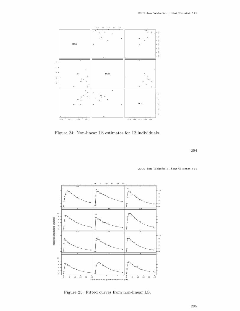
Exploratory Plots/Analyses

> library(nlme); data(Theoph); (Theoph)

> TheoSTS.nls <- nlsList(conc~SSfol(Dose, Time, lKe, lKa, lCl),data=Theoph)

> TheoSTS.nls

Model: conc ~ SSfol(Dose, Time, lKe, lKa, lCl) | Subject

Coefficients:

lKe lKa lCl

6 -2.307332 0.1516234 -2.973242

7 -2.280370 -0.3860511 -2.964335

8 -2.386437 0.3188339 -3.069111

11 -2.321530 1.3478239 -2.860397

3 -2.508073 0.8975422 -3.229965

2 -2.286108 0.6640568 -3.106317

4 -2.436494 0.1582638 -3.286087

9 -2.446088 2.1821879 -3.420774

12 -2.248326 -0.1828442 -3.170158

10 -2.604148 -0.3631216 -3.428271

1 -2.919614 0.5751612 -3.915857

5 -2.425486 0.3862853 -3.132600

Degrees of freedom: 132 total; 96 residual

Residual standard error: 0.7001921

> plot(intervals(TheoSTS.nls))

> pairs(coef(TheoSTS.nls))

> plot(augPred(TheoSTS.nls))

293


lKe

0.0 0.5 1.0 1.5 2.0

−2.9

−2.8

−2.7

−2.6

−2.5

−2.4

−2.3

0.00.5

1.01.5

2.0

lKa

−2.9 −2.7 −2.5 −2.3 −3.8 −3.6 −3.4 −3.2 −3.0

−3.8

−3.6

−3.4

−3.2

−3.0

lCl

Figure 24: Non-linear LS estimates for 12 individuals.

294



Theo

phyll

ine co

ncen

tratio

n in s

erum

(mg/l

)

0

2

4

6

8

10

0 5 10 15 20 25

6 7

0 5 10 15 20 25

8

11 3

0

2

4

6

8

10

2

0

2

4

6

8

10

4 9 12

10

0 5 10 15 20 25

1

0

2

4

6

8

10

5

Figure 25: Fitted curves from non-linear LS.

295


Likelihood Inference for the NLMEM

See Pinheiro and Bates (2000, Chapter 7).

The likelihood is, as usual, obtained by integrating out the random effects:

L(β, α) = (2πσ2ǫ )−N/2(2π)−m/2|D|−m/2

×mY

i=1

Zexp

»− (yi − fi)

T(yi − fi)

2σ2ǫ

− bTi D−1bi

2

–dbi.

where fi is made up of terms f(ηij , tij), i = 1, ..., m, j = 1, ..., ni.

296


Laplace Approximation in the NLMEM

See Pinheiro and Bates, Chapter 7.

We wish to evaluate

p(yi | β, α) = (2πσ2)−ni/2(2π)−(q+1)/2 | D |−1/2

Zexp{nig(bi)} dbi,

where

−2nig(bi) = [yi − fi(β, bi, xi)]T[yi − fi(β, bi, xi)]/σ2

ǫ + bTi D−1bi.

A Laplace approximation is a second-order Taylor series expansion of g about

bbi = arg minbi

−g(bi)

which will not be available in closed form for a non-linear model.

297


The nlme algorithm

Within nlme an algorithm, introduced by Lindstrom and Bates (1990) is used.

The algorithm alternates between two steps:

Penalized Non-linear Least Squares (PNLS)

Condition on the current estimates of bD and bσ2ǫ and then minimize

1

bσ2ǫ

mX

i=1

(yi − fi)T(yi − fi) + bi

bD−1bi,

to obtain estimates bβ,bb1, ...,bbm, which may be viewed as finding the posterior

mode for β and b1, ..., bm.

298


Linear Mixed Effects (LME)

Carry out a first-order Taylor series of fi about bβ,bbi.

This results in a linear mixed effects model which can be maximized to obtain

estimates of D and σ2ǫ .

We have likelihood

L(β, α) =| D |−m/2 σ−Nǫ

Zexp

(−1

2

mX

i=1

(yi − fi)T(yi − fi) − bT

i D−1bi

)dbi

where fi = f(β, bi, xi), i = 1, ..., m.

Carry out a first-order Taylor series expansion of fi about the estimates,

obtained in the PNLS step at iteration k, of β and bi, call these bβ(k)and bb(k)

i .

299


Specifically

fi(β, bi) ≈ f

i

“bβ(k)

,bb(k)

i

”+ bx(k)

i

“β −

bβ(k)”

+ bz(k)i

“bi −

bbi

(k)”

where

bx(k)i =

∂fi

∂βT

˛̨˛̨

bβ(k)

,bb(k)

i

bz(k)i =

∂fi

∂bTi

˛̨˛̨

bβ(k)

,bb(k)

i

This gives

yi− f

i(β, bi) ≈ y

(k)i

− bx(k)i

β − bz(k)i

bi

where

y(k)i

= yi− f

i

“bβ(k)

,bb(k)

i

”+ bx(k)

ibβ(k)

+ bz(k)i

bb(k)

i

300


The integral can now be evaluated in closed-form to give the log-likelihood

l(α) = −1

2

mX

i=1

log | bV i| −1

2

mX

i=1

(y(k)i − bx(k)

i β)T bV −1i (Y i − bxiβ)

wherebV i = bz(k)

i Dbz(k)Ti + σ2

ǫ Ii,

which may be maximized to give ML estimates. REML estimates are obtained

by adding the term

−1

2

mX

i=1

log | bx(k)Ti

bV i(α)bx(k)i |

The Laplace approximation is generally more accurate than the LB algorithm,

it is, however, more computationally expensive.

301


Asymptotic Inference

Under the LB algorithm, the asymptotic distribution of the REML estimator bβis

mX

i=1

bxTibV −1

i bxi

!1/2

(bβ − β) →d Np+1(0, Ip+1),

where bxi = bx(k)i with k the final iteration, i = 1, ..., m

Similarly, the asymptotic distribution of α is based on the information as

calculated from the linear approximation to the likelihood.

The LB estimator is inconsistent if the ni’s are fixed and m → ∞.

Empirical Bayes estimates for the random effects are available, but caution

should be given to using these for checking assumptions since they are strongly

influenced by the assumption of normality being correct. If ni is large then this

will be less of a problem.

302


Approaches for NLMEMs

Various other approaches to likelihood inference have been suggested, we briefly

summarize.

In general we need to carry out m integrals of dimension q + 1 for each

likelihood evaluation, so with large m and q this can be computationally

expensive.

First-Order Approximation

Let βi = xiβ + bi, and then carry out a first-order Taylor series about

E[bi] = 0 to give

yi = fi(βi) + ǫi ≈ fi(xiβ) +∂fi

∂βi

∂βi

∂bibi + ǫi.

In contrast to the LB algorithm which considered an expansion about the

subject-specific mean, the expansion here is about the population-averaged

mean. The first-order estimator is inconsistent and has bias even if ni and m

go to infinity, see Demidenko (2004, Chapter 8)

Adaptive Gaussian quadrature may also be used.

303


Example: NLMEM for Pharmacokinetics of Theophylline

> Theo.nlme <- nlme(TheoSTS.nls,fixed=lKe+lKa+lCl~1,random=lKe+lKa+lCl~1,data=Theoph)

> summary(Theo.nlme)

Nonlinear mixed-effects model fit by maximum likelihood

Model: conc ~ SSfol(Dose, Time, lKe, lKa, lCl) Random effects:

Formula: list(lKe ~ 1, lKa ~ 1, lCl ~ 1)

Structure: General positive-definite, Log-Cholesky parametrization

StdDev Corr

lKe 0.1310435 lKe lKa

lKa 0.6377804 0.012

lCl 0.2511766 0.995 -0.089

Residual 0.6818265

Fixed effects: list(lKe ~ 1, lKa ~ 1, lCl ~ 1)

Value Std.Error DF t-value p-value

lKe -2.432671 0.06302415 118 -38.59903 0.0000

lKa 0.451410 0.19624487 118 2.30024 0.0232

lCl -3.214452 0.08059540 118 -39.88382 0.0000

Correlation:

lKe lKa

lKa -0.143

lCl 0.854 -0.131

Number of Observations: 132 Number of Groups: 12

> plot(augPred(Theo.nlme))

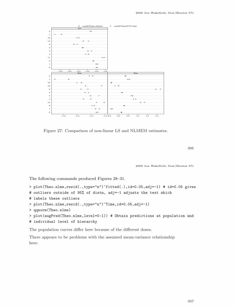
> plot(compareFits(coef(Theo.nlme), coef(TheoSTS.nls)))

304



Theoph

ylline c

oncent

ration

in seru

m (mg

/l)

0

2

4

6

8

10

0 5 10 15 20 25

6 7

0 5 10 15 20 25

8

11 3

0

2

4

6

8

10

2

0

2

4

6

8

10

4 9 12

10

0 5 10 15 20 25

1

0

2

4

6

8

10

5

Figure 26: Fitted curves from NLMEM fit.

305


6

7

8

11

3

2

4

9

12

10

1

5

−2.8 −2.6 −2.4 −2.2

lKe

−0.5 0.0 0.5 1.0 1.5 2.0

lKa

6

7

8

11

3

2

4

9

12

10

1

5

−3.8 −3.6 −3.4 −3.2 −3.0 −2.8

lCl

coef(Theo.nlme) coef(TheoSTS.nls)

Figure 27: Comparison of non-linear LS and NLMEM estimates.

306


The following commands produced Figures 28–31.

> plot(Theo.nlme,resid(.,type="n")~fitted(.),id=0.05,adj=-1) # id=0.05 gives

# outliers outside of 95% of distn, adj=-1 adjusts the text which

# labels these outliers

> plot(Theo.nlme,resid(.,type="n")~Time,id=0.05,adj=-1)

> qqnorm(Theo.nlme)

> plot(augPred(Theo.nlme,level=0:1)) # Obtain predictions at population and

# individual level of hierarchy

The population curves differ here because of the different doses.

There appears to be problems with the assumed mean-variance relationship

here.

307


Fitted values (mg/l)

Standa

rdized

residu

als

−2

0

2

4

0 2 4 6 8 10

1

2

2

4

4

5

5

8

9

12

Figure 28: Standardized residuals versus fitted values.

308



Standa

rdized

residu

als

−2

0

2

4

0 5 10 15 20 25

1

2

2

4

4

5

5

8

9

12

Figure 29: Standardized residuals versus time.

309


Standardized residuals

Quant

iles of

standa

rd nor

mal

−2

−1

0

1

2

−2 0 2 4

Figure 30: QQ plot of normalized residuals.

310



Theop

hylline

conce

ntratio

n in se

rum (m

g/l)

0

2

4

6

8

10

0 5 10 15 20 25

6 7

0 5 10 15 20 25

8

11 3

0

2

4

6

8

10

2

0

2

4

6

8

10

4 9 12

10

0 5 10 15 20 25

1

0

2

4

6

8

10

5

fixed Subject

Figure 31: Solid lines are population predictions, dashed lines individual predic-

tions.

311


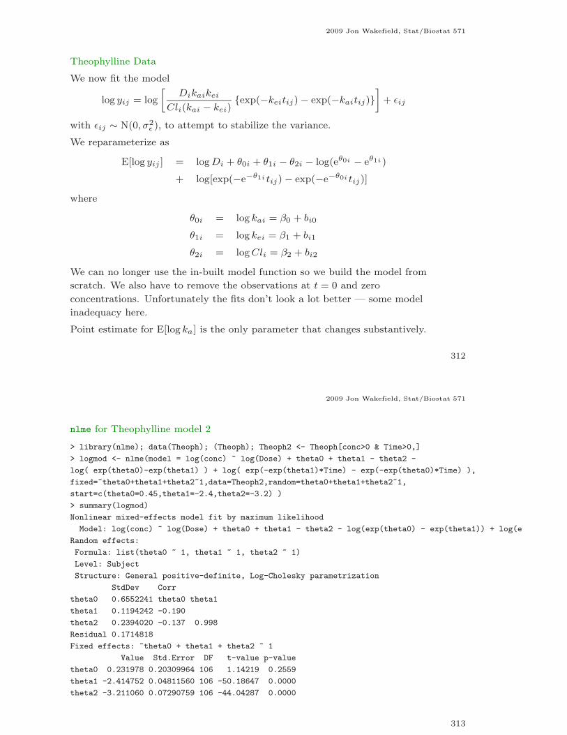
Theophylline Data

We now fit the model

log yij = log

»Dikaikei

Cli(kai − kei){exp(−keitij) − exp(−kaitij)}

–+ ǫij

with ǫij ∼ N(0, σ2ǫ ), to attempt to stabilize the variance.

We reparameterize as

E[log yij ] = log Di + θ0i + θ1i − θ2i − log(eθ0i − eθ1i)

+ log[exp(−e−θ1i tij) − exp(−e−θ0i tij)]

where

θ0i = log kai = β0 + bi0

θ1i = log kei = β1 + bi1

θ2i = log Cli = β2 + bi2

We can no longer use the in-built model function so we build the model from

scratch. We also have to remove the observations at t = 0 and zero

concentrations. Unfortunately the fits don’t look a lot better — some model

inadequacy here.

Point estimate for E[log ka] is the only parameter that changes substantively.

312


nlme for Theophylline model 2

> library(nlme); data(Theoph); (Theoph); Theoph2 <- Theoph[conc>0 & Time>0,]

> logmod <- nlme(model = log(conc) ~ log(Dose) + theta0 + theta1 - theta2 -

log( exp(theta0)-exp(theta1) ) + log( exp(-exp(theta1)*Time) - exp(-exp(theta0)*Time) ),

fixed=~theta0+theta1+theta2~1,data=Theoph2,random=theta0+theta1+theta2~1,

start=c(theta0=0.45,theta1=-2.4,theta2=-3.2) )

> summary(logmod)

Nonlinear mixed-effects model fit by maximum likelihood

Model: log(conc) ~ log(Dose) + theta0 + theta1 - theta2 - log(exp(theta0) - exp(theta1)) + log(exp(-exp(theta1)

Random effects:

Formula: list(theta0 ~ 1, theta1 ~ 1, theta2 ~ 1)

Level: Subject

Structure: General positive-definite, Log-Cholesky parametrization

StdDev Corr

theta0 0.6552241 theta0 theta1

theta1 0.1194242 -0.190

theta2 0.2394020 -0.137 0.998

Residual 0.1714818

Fixed effects: ~theta0 + theta1 + theta2 ~ 1

Value Std.Error DF t-value p-value

theta0 0.231978 0.20309964 106 1.14219 0.2559

theta1 -2.414752 0.04811560 106 -50.18647 0.0000

theta2 -3.211060 0.07290759 106 -44.04287 0.0000

313


Fitted values (mg/l)

Standa

rdized

residu

als

−3

−2

−1

0

1

2

3

0.0 0.5 1.0 1.5 2.0

2

2

4

4

5

5

78

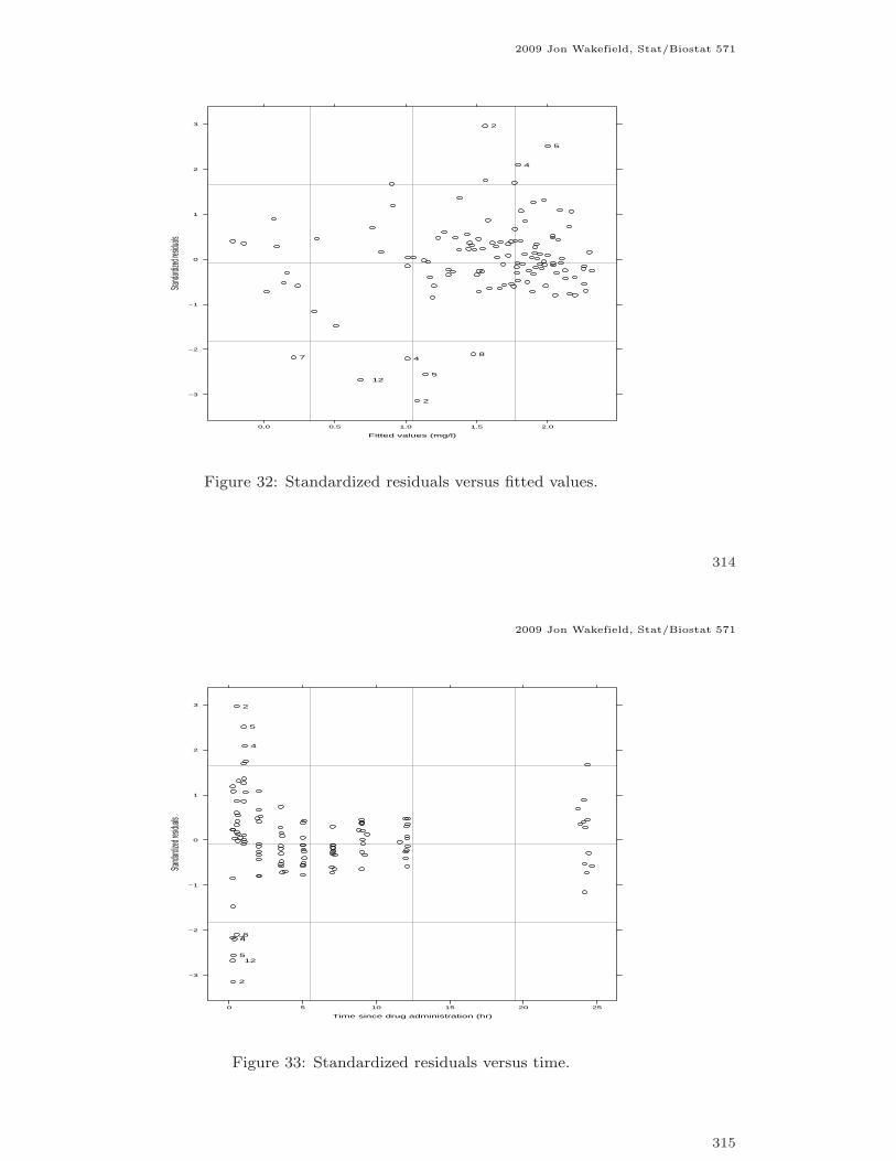
12

Figure 32: Standardized residuals versus fitted values.

314



Standa

rdized

residu

als

−3

−2

−1

0

1

2

3

0 5 10 15 20 25

2

2

4

4

5

5

78

12

Figure 33: Standardized residuals versus time.

315


Standardized residuals

Quant

iles of

standa

rd nor

mal

−2

−1

0

1

2

−3 −2 −1 0 1 2 3

Figure 34: QQ plot of normalized residuals.

316


Bayesian Approach

A Bayesian approach adds a prior distribution for β, α, to the likelihood

L(β, α). As with the linear model proper prior is required for the matrix D. In

general a proper prior is required for β also, to ensure the propriety of the

posterior distribution. Closed-form inference is unavailable, but MCMC is

almost as straightforward as in the LMEM case. The joint posterior is

p(β1, ..., βm, τ, β, W , b | y) ∝mY

i=1

{p(yi | βi, τ)p(βi | β, W)}π(β)π(τ)π(W).

Suppose we have priors:

β ∼ Nq+1(β0, V 0)

τ ∼ Ga(a0, b0)

W ∼ Wq+1(r, R−1)

The conditional distributions for β, τ , W are unchanged from the linear case.

There is no closed form conditional distribution for βi, which is given by:

p(βi | β, τ, W , y) ∝ p(yi | βi, τ) × p(βi | β, W)

but a Metropolis-Hastings step can be used.

317


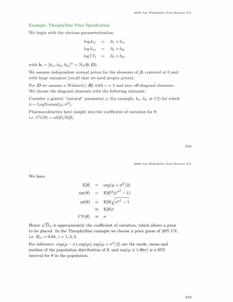
Example: Theophylline Prior Specification

We begin with the obvious parameterization:

log kei = β1 + b1i

log kai = β2 + b2i

log Cli = β3 + b3i

with bi = [b1i, b2i, b3i]T ∼ N3(0, D).

We assume independent normal priors for the elements of β, centered at 0 and

with large variances (recall that we need proper priors).

For D we assume a Wishart(r, R) with r = 3 and zero off-diagonal elements.

We choose the diagonal elements with the following rationale.

Consider a generic “natural” parameter φ (for example, ke, ka or Cl) for which

φ ∼ LogNormal(µ, σ2).

Pharmacokinetics have insight into the coefficient of variation for θ,

i.e. CV(θ) = sd(θ)/E[θ].

318


We have

E[θ] = exp(µ + σ2/2)

var(θ) = E[θ]2(eσ2 − 1)

sd(θ) = E[θ]

qeσ2 − 1

≈ E[θ]σ

CV(θ) ≈ σ

Hence√

Dii is approximately the coefficient of variation, which allows a prior

to be placed. In the Theophylline example we choose a prior guess of 20% CV,

i.e. Rii = 0.04, i = 1, 2, 3.

For inference: exp(µ − σ), exp(µ), exp(µ + σ2/2) are the mode, mean and

median of the population distribution of θ, and exp(µ ± 1.96σ) is a 95%

interval for θ in the population.

319


Functions of Interest

In pharamacokinetics there is interest in quantities such as the terminal half-life

t1/2 =log 2

ke

Since log ke ∼ N(β1, D11),

log t1/2 ∼ N(log[log 2] − β1, D11)

Other parameters are not simple linear combinations, e.g. time to maximum

tmax =1

ka − kelog

„ka

ke

«

and the maximum concentration

E[Y |tmax] =Dka

V (ka − ke){exp(−ketmax) − exp(−katmax)}

=D

V

„ka

ke

«ka/(ka−ke)

.

320


WinBUGS for Theophylline

model

{

for( i in 1 : N ) {

for( j in 1 : T ) {

Y[i , j] ~ dnorm(mu[i , j],eps.tau)

mu[i , j] <- Dose[i]*exp(theta[i,1] + theta[i,2] - theta[i,3]) *

(exp(-exp(theta[i,1])*time[i,j]) - exp(-exp(theta[i,2])*time[i,j]) )/

(exp(theta[i,2])-exp(theta[i,1]))

}

theta[i, 1:3] ~ dmnorm(beta[1:3], Dinv[1:3, 1:3])

ke[i] <- exp(theta[i,1])

ka[i] <- exp(theta[i,2])

Cl[i] <- exp(theta[i,3])

}

eps.tau <- exp(logtau)

logtau ~ dflat()

sigma <- 1 / sqrt(eps.tau)

beta[1:3] ~ dmnorm(mean[1:3], prec[1:3, 1:3])

kemed <- exp(beta[1])

kamed <- exp(beta[2])

Clmed <- exp(beta[3])

Dinv[1:3, 1:3] ~ dwish(R[1:3, 1:3], 3)

D[1:3, 1:3] <- inverse(Dinv[1:3, 1:3])

321


for (i in 1 : 3) {sdD[i] <- sqrt(D[i, i]) }

}

DATA

list( N = 12, T = 11,Dose=c(4.02,4.4,4.53,4.4,5.86,4,4.95,4.53,3.1,5.5,4.92,5.3),

Y = structure(.Data = c(0.74,2.84,6.57,10.50,...,4.57,1.17),

.Dim = c(12,11)),

time = structure(.Data = c(0.00,0.25, ...,7.07,9.03,12.05,24.15),.Dim = c(12,11)),

mean = c(0,0,0),R = structure(.Data = c(0.2, 0, 0,0, 0.2, 0,0, 0, 0.2), .Dim = c(3, 3)),

prec = structure(.Data = c(1.0E-6,0,0,0,1.0E-6,0,0,0,1.0E-6),.Dim = c(3, 3)))

INITS

list(theta = structure(.Data = c(-2.2,0,3,-2.2,0,3,-2.2,0,3,-2.2,0,3,-2.2,0,3,-2.2,

0,3,-2.2,0,3,-2.2,0,3,-2.2,0,3,-2.2,0,3,-2.2,0,3,-2.2,0,3), .Dim = c(12, 3)),

beta = c(-2, .1, -3), Dinv = structure(.Data = c(1, 0, 0,0, 1, 0,0, 0, 1), .Dim = c(3, 3)),

logtau = 0)

The first time this model was run with two chains the second chain flipped

between two non-identifiable regions in the parameter space

322


Figure 35: Demonstration of flip-flop behavior.

323


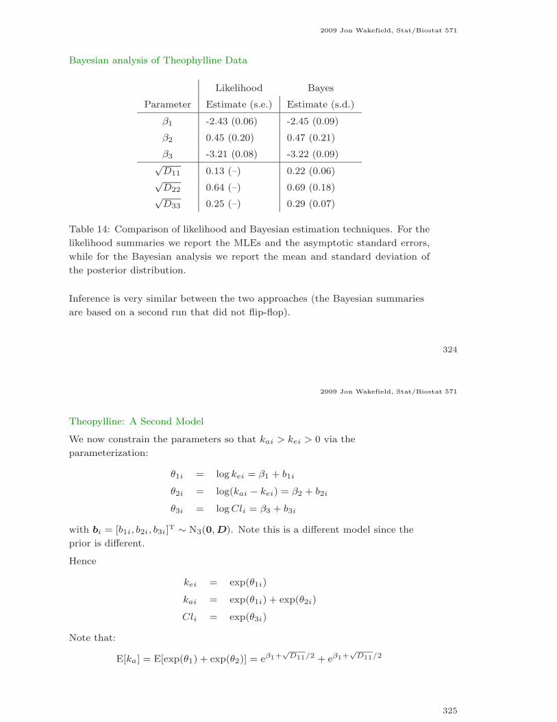
Bayesian analysis of Theophylline Data

Likelihood Bayes

Parameter Estimate (s.e.) Estimate (s.d.)

β1 -2.43 (0.06) -2.45 (0.09)

β2 0.45 (0.20) 0.47 (0.21)

β3 -3.21 (0.08) -3.22 (0.09)√

D11 0.13 (–) 0.22 (0.06)√

D22 0.64 (–) 0.69 (0.18)√

D33 0.25 (–) 0.29 (0.07)

Table 14: Comparison of likelihood and Bayesian estimation techniques. For the

likelihood summaries we report the MLEs and the asymptotic standard errors,

while for the Bayesian analysis we report the mean and standard deviation of

the posterior distribution.

Inference is very similar between the two approaches (the Bayesian summaries

are based on a second run that did not flip-flop).

324


Theopylline: A Second Model

We now constrain the parameters so that kai > kei > 0 via the

parameterization:

θ1i = log kei = β1 + b1i

θ2i = log(kai − kei) = β2 + b2i

θ3i = log Cli = β3 + b3i

with bi = [b1i, b2i, b3i]T ∼ N3(0, D). Note this is a different model since the

prior is different.

Hence

kei = exp(θ1i)

kai = exp(θ1i) + exp(θ2i)

Cli = exp(θ3i)

Note that:

E[ka] = E[exp(θ1) + exp(θ2)] = eβ1+√

D11/2 + eβ1+√

D11/2

325


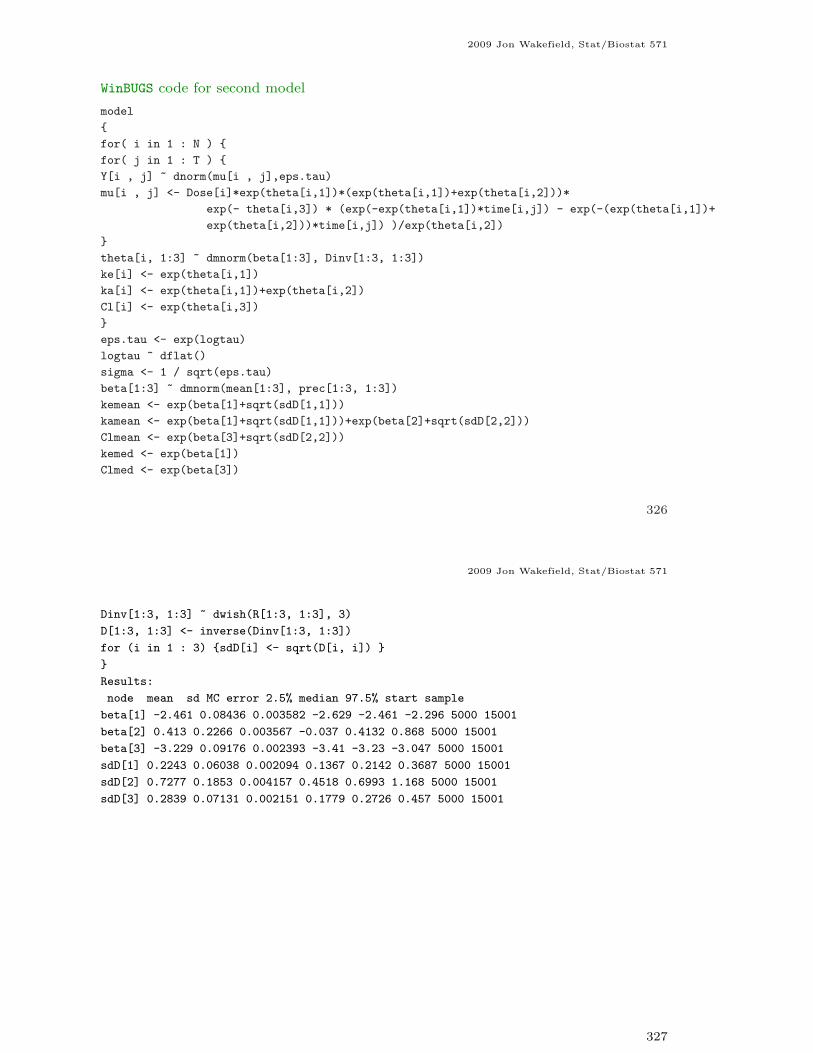
WinBUGS code for second model

model

{

for( i in 1 : N ) {

for( j in 1 : T ) {

Y[i , j] ~ dnorm(mu[i , j],eps.tau)

mu[i , j] <- Dose[i]*exp(theta[i,1])*(exp(theta[i,1])+exp(theta[i,2]))*

exp(- theta[i,3]) * (exp(-exp(theta[i,1])*time[i,j]) - exp(-(exp(theta[i,1])+

exp(theta[i,2]))*time[i,j]) )/exp(theta[i,2])

}

theta[i, 1:3] ~ dmnorm(beta[1:3], Dinv[1:3, 1:3])

ke[i] <- exp(theta[i,1])

ka[i] <- exp(theta[i,1])+exp(theta[i,2])

Cl[i] <- exp(theta[i,3])

}

eps.tau <- exp(logtau)

logtau ~ dflat()

sigma <- 1 / sqrt(eps.tau)

beta[1:3] ~ dmnorm(mean[1:3], prec[1:3, 1:3])

kemean <- exp(beta[1]+sqrt(sdD[1,1]))

kamean <- exp(beta[1]+sqrt(sdD[1,1]))+exp(beta[2]+sqrt(sdD[2,2]))

Clmean <- exp(beta[3]+sqrt(sdD[2,2]))

kemed <- exp(beta[1])

Clmed <- exp(beta[3])

326


Dinv[1:3, 1:3] ~ dwish(R[1:3, 1:3], 3)

D[1:3, 1:3] <- inverse(Dinv[1:3, 1:3])

for (i in 1 : 3) {sdD[i] <- sqrt(D[i, i]) }

}

Results:

node mean sd MC error 2.5% median 97.5% start sample

beta[1] -2.461 0.08436 0.003582 -2.629 -2.461 -2.296 5000 15001

beta[2] 0.413 0.2266 0.003567 -0.037 0.4132 0.868 5000 15001

beta[3] -3.229 0.09176 0.002393 -3.41 -3.23 -3.047 5000 15001

sdD[1] 0.2243 0.06038 0.002094 0.1367 0.2142 0.3687 5000 15001

sdD[2] 0.7277 0.1853 0.004157 0.4518 0.6993 1.168 5000 15001

sdD[3] 0.2839 0.07131 0.002151 0.1779 0.2726 0.457 5000 15001

327


Generalized Estimating Equations

If interest lies in population parameters then we may use the estimator bβ that

satisfies

G(β, bα) =mX

i=1

DTi W−1

i (Y i − µi) = 0,

where Di = ∂µi

∂β, W i = W i(β, bα) is the working covariance model, µi = µi(β)

and bα is a consistent estimator of α. Sandwich estimation may be used to

obtain an empirical estimate of the variance, V β :

mX

i=1

DTi W−1

i Di

!−1( mX

i=1

DTi W−1

i cov(Y i)W−1i Di

) mX

i=1

DTi W−1

i Di

!−1

.

We then have

V−1/2β (bβ − β) →d N(0, I).

In practice an empirical estimator of cov(Y i) is substituted to give bV β .

GEE has not been extensively used in a non-linear (non-GLM) setting. This is

probably because in many settings (e.g. pharmacokinetic/pharmacodynamic)

interest focuses on understanding between individual-variability, and explaining

this in terms of individual-specific covariates.

328

logistic mixed effects models a glmm for binary data takes the

Documents