logic, reasoning, and uncertainty - university of washington

Logic, Reasoning, and UncertaintyLogic, Reasoning, and Uncertainty

CSEP 573

© CSE AI Faculty

2

What’s on our menu today?What’s on our menu today?Propositional Logic

• Resolution• WalkSAT

Reasoning with First-Order Logic• Unification• Forward/Backward Chaining• Resolution• Wumpus again

Uncertainty• Bayesian networks

3

Recall from Last Time: Inference/Proof Techniques

Recall from Last Time: Inference/Proof Techniques

Two kinds (roughly):Successive application of inference rules

– Generate new sentences from old in a sound way– Proof = a sequence of inference rule applications– Use inference rules as successor function in a

standard search algorithm– E.g., Resolution

Model checking– Done by checking satisfiability: the SAT problem– Recursive depth-first enumeration of models using heuristics: DPLL algorithm (sec. 7.6.1 in text)

– Local search algorithms (sound but incomplete)e.g., randomized hill-climbing (WalkSAT)

4

Understanding ResolutionUnderstanding ResolutionIDEA: To show KB ╞ α, use proof by contradiction, i.e., show KB ∧ ¬ α unsatisfiable

KB is in Conjunctive Normal Form (CNF):KB is conjunction of clauses

E.g., (A ∨ ¬B) ∧ (B ∨ ¬C ∨ ¬D)

Literals

Clause

5

Generating new clausesGenerating new clausesGeneral Resolution inference rule (for CNF):

l1 ∨… ∨ l k m1 ∨ … ∨ mn

l1 ∨ … ∨ li-1 ∨ li+1 ∨ … ∨ l k ∨ m1 ∨ … ∨ mj-1 ∨ mj+1…∨ mn

where li and mj are complementary literals (l i = ¬mj)

E.g., P1,3 ∨ P2,2 ¬P2,2

P1,3

6

Why this is soundWhy this is soundProof of soundness of resolution inference rule:

¬ (l1 ∨ … ∨ li-1 ∨ li+1 ∨ … ∨ l k) ⇒ l i¬mj ⇒ (m1 ∨ … ∨ mj-1 ∨ mj+1 ∨... ∨ mn)

¬ (li ∨ … ∨ li-1 ∨ li+1 ∨ … ∨ lk) ⇒ (m1 ∨ … ∨ mj-1 ∨mj+1 ∨... ∨ mn)

(since l i = ¬mj)

7

Resolution exampleResolution example

Empty clause

Recall that KB is a conjunction of all these clauses

Is P1,2 ∧ ¬P1,2 satisfiable? No!

Therefore, KB ∧ ¬ α is unsatisfiable, i.e., KB ╞ α

You got a literal and its negationWhat does this mean?

KB ¬α

8

Back to Inference/Proof TechniquesBack to Inference/Proof Techniques

Two kinds (roughly):Successive application of inference rules

– Generate new sentences from old in a sound way– Proof = a sequence of inference rule applications– Use inference rules as successor function in a

standard search algorithm– E.g., Resolution

Model checking– Done by checking satisfiability: the SAT problem– Recursive depth-first enumeration of models using heuristics: DPLL algorithm (sec. 7.6.1 in text)

– Local search algorithms (sound but incomplete)e.g., randomized hill-climbing (WalkSAT)

9

Why Satisfiability?Why Satisfiability?

Can’t get¬satisfaction

10

Why Satisfiability?Why Satisfiability?Recall: KB ╞ α iff KB ∧ ¬α is unsatisfiableThus, algorithms for satisfiability can be used for inference by showing KB ∧ ¬α is unsatisfiable

BUT… showing a sentence is satisfiable (the SAT problem)

is NP-complete!Finding a fast algorithm for SAT

automatically yields fast algorithms for hundreds of difficult (NP-

complete) problems

I really can’t get¬satisfaction

11

Satisfiability ExamplesSatisfiability Examples

E.g. 2-CNF sentences (2 literals per clause):

(¬A ∨ ¬B) ∧ (A ∨ B) ∧ (A ∨ ¬B)Satisfiable?Yes (e.g., A = true, B = false)

(¬A ∨ ¬B) ∧ (A ∨ B) ∧ (A ∨ ¬B) ∧ (¬A ∨ B)Satisfiable?No

12

The WalkSAT algorithmThe WalkSAT algorithmLocal hill climbing search algorithm

• Incomplete: may not always find a satisfying assignment even if one exists

Evaluation function? = Number of satisfied clauses

WalkSAT tries to maximize this function

Balance between greediness and randomness

13

The WalkSAT algorithmThe WalkSAT algorithm

Greed Randomness

14

Hard Satisfiability ProblemsHard Satisfiability ProblemsConsider random 3-CNF sentences. e.g.,(¬D ∨ ¬B ∨ C) ∧ (B ∨ ¬A ∨ ¬C) ∧ (¬C ∨ ¬B ∨ E) ∧(E ∨ ¬D ∨ B) ∧ (B ∨ E ∨ ¬C)

m = number of clauses n = number of symbols

• Hard instances of SAT seem to cluster near m/n = 4.3 (critical point)

15

Hard Satisfiability ProblemsHard Satisfiability Problems

16

Hard Satisfiability ProblemsHard Satisfiability Problems

Median runtime for random 3-CNF sentences, n = 50

What about me?What about me?

18

Putting it all together:Logical Wumpus AgentsPutting it all together:Logical Wumpus Agents

A wumpus-world agent using propositional logic:¬P1,1

¬W1,1

For x = 1, 2, 3, 4 and y = 1, 2, 3, 4, add (with appropriate boundary conditions):Bx,y ⇔ (Px,y+1 ∨ Px,y-1 ∨ Px+1,y ∨ Px-1,y) Sx,y ⇔ (Wx,y+1 ∨ Wx,y-1 ∨ Wx+1,y ∨ Wx-1,y)

W1,1 ∨ W1,2 ∨ … ∨ W4,4

¬W1,1 ∨ ¬W1,2

¬W1,1 ∨ ¬W1,3

…⇒ 64 distinct proposition symbols, 155 sentences!

At most 1 wumpus

At least 1 wumpus

19

KB contains "physics" sentences for every single square

For every time step t and every location [x,y], we need to add to the KB:

Lx,y ∧ FacingRight t ∧ Forward t ⇒ Lx+1,y

Rapid proliferation of sentences!

t+1t

Limitations of propositional logicLimitations of propositional logic

What we’d like is a way to talk about objects and groups of objects, and to

define relationships between them

What we’d like is a way to talk about objects and groups of objects, and to

define relationships between them

Enter…First-Order Logic

(aka “Predicate logic”)

21

Propositional vs. First-OrderPropositional vs. First-OrderPropositional logic

Facts: p, q, ¬r, ¬P1,1, ¬W1,1 etc.(p ∧ q) v (¬r v q ∧ p)

First-order logicObjects: George, Monkey2, Raj, 573Student1, etc.Relations:

Curious(George), Curious(573Student1), …Smarter(573Student1, Monkey2)Smarter(Monkey2, Raj)Stooges(Larry, Moe, Curly)PokesInTheEyes(Moe, Curly)PokesInTheEyes(573Student1, Raj)

22

FOL DefinitionsConstants: George, Monkey2, etc.

• Name a specific object. Variables: X, Y.

• Refer to an object without naming it.Functions: banana-of, grade-of, etc.

• Mapping from objects to objects.Terms: banana-of(George), grade-of(stdnt1)

• Logical expressions referring to objectsRelations (predicates): Curious, PokesInTheEyes, etc.

• Properties of/relationships between objects.

23

Logical connectives: and, or, not, ⇒, ⇔Quantifiers:

• ∀ For all (Universal quantifier)• ∃ There exists (Existential quantifier)

Examples• George is a monkey and he is curious

• All monkeys are curious

• There is a curious monkey

More Definitions

Monkey(George) ∧ Curious(George)

∀m: Monkey(m) ⇒ Curious(m)

∃m: Monkey(m) ∧ Curious(m)

24

Quantifier / Connective Interaction

Quantifier / Connective Interaction

∀x: M(x) ∧ C(x)

∀x: M(x) ⇒C(x)

∃x: M(x) ∧ C(x)

∃x: M(x) ⇒ C(x)

M(x) == “x is a monkey”C(x) == “x is curious”

“Everything is a curious monkey”

“All monkeys are curious”

“There exists a curious monkey”

“There exists an object that is either a curiousmonkey, or not a monkey at all”

25

Nested Quantifiers: Order matters!

Nested Quantifiers: Order matters!

ExamplesEvery monkey has a tail

∀x ∃y P(x,y) ≠ ∃y ∀x P(x,y)

∀m ∃t has(m,t)

Everybody loves somebody vs. Someone is loved by everyone

∃t ∀m has(m,t)

Every monkey shares a tail!

Try:

∃y ∀x loves(x, y)∀x ∃y loves(x, y)

26

SemanticsSemantics = what the arrangement of symbols means in the world

Propositional logic• Basic elements are variables

(refer to facts about the world)• Possible worlds: mappings from variables to T/F

First-order logic• Basic elements are terms

(logical expressions that refer to objects)• Interpretations: mappings from terms to real-world elements.

27

Example: A World of Kings and LegsExample: A World of Kings and Legs

Syntactic elements:

Richard JohnConstants: Functions: Relations:

• LeftLeg(p) On(x,y) King(p)

28

Interpretation IInterpretation IInterpretations map syntactic tokens to model elements

• Constants: Functions: Relations:•

Richard John LeftLeg(p) On(x,y) King(p)

29

Interpretation IIInterpretation II• Constants: Functions: Relations:•Richard John LeftLeg(p) On(x,y) King(p)

30

Two constants (and 5 objects in world)

• Richard, John (R, J, crown, RL, JL)

One unary relationKing(x)

Two binary relations• Leg(x, y); On(x, y)

How Many Interpretations?How Many Interpretations?

52 = 25 object mappings

Infinite number of values for x infinite mappingsEven if we restricted x to: R, J, crown, RL, JL:

25 = 32 unary truth mappings

Infinite. But even restricting x, y to five objects still yields 225 mappings for each binary relation

31

Satisfiability, Validity, & Entailment

Satisfiability, Validity, & Entailment

S is valid if it is true in all interpretations

S is satisfiable if it is true in some interp

S is unsatisfiable if it is false in all interps

S1 ╞ S2 (S1 entails S2) if For all interps where S1 is true, S2 is also true

32

Propositional. Logic vs. First Order

Ontology

Syntax

Semantics

InferenceAlgorithm

Complexity

Objects, Properties, Relations

Atomic sentencesConnectives

Variables & quantificationSentences have structure: termsfather-of(mother-of(X)))

UnificationForward, Backward chaining Prolog, theorem proving

DPLL, WalkSATFast in practice

Semi-decidableNP-Complete

Facts (P, Q,…)

Interpretations (Much more complicated)Truth Tables

33

First-Order Wumpus WorldFirst-Order Wumpus WorldObjects

• Squares, wumpuses, agents,• gold, pits, stinkiness, breezes

Relations• Square topology (adjacency),• Pits/breezes,• Wumpus/stinkiness

34

Wumpus World: SquaresWumpus World: Squares

Better: Squares as lists:[1, 1], [1,2], …, [4, 4]

Square topology relations:∀x, y, a, b: Adjacent([x, y], [a, b])

[a, b] Є {[x+1, y], [x-1, y], [x, y+1], [x, y-1]}

• Each square as an object:Square1,1, Square1,2, …, Square3,4, Square4,4

•Square topology relations?Adjacent(Square1,1, Square2,1)…Adjacent(Square3,4, Square4,4)

35

Wumpus World: PitsWumpus World: Pits•Each pit as an object:

Pit1,1, Pit1,2, …, Pit3,4, Pit4,4

• Problem?Not all squares have pits

List only the pits we have?Pit3,1, Pit3,3, Pit4,4

Problem?No reason to distinguish pits (same properties)

Better: pit as unary predicatePit(x)Pit([3,1]); Pit([3,3]); Pit([4,4]) will be true

36

Wumpus World: BreezesWumpus World: Breezes

“Squares next to pits are breezy”:∀x, y, a, b:Pit([x, y]) ∧ Adjacent([x, y], [a, b]) ⇒ Breezy([a, b])

• Represent breezes like pits,as unary predicates:

Breezy(x)

37

Wumpus World: WumpusesWumpus World: Wumpuses

Better: Wumpus’s home as a function:Home(Wumpus) references the wumpus’s home square.

• Wumpus as object:Wumpus

• Wumpus home as unary predicate:

WumpusIn(x)

38

FOL Reasoning: OutlineFOL Reasoning: OutlineBasics of FOL reasoningClasses of FOL reasoning methods

• Forward & Backward Chaining • Resolution• Compilation to SAT

39

Universally quantified sentence:• ∀x: Monkey(x) ⇒ Curious(x)

Intutively, x can be anything:• Monkey(George) ⇒ Curious(George)

• Monkey(473Student1) ⇒ Curious(473Student1)

• Monkey(DadOf(George)) ⇒ Curious(DadOf(George))

Formally: (example)∀x S ∀x Monkey(x) Curious(x)

Subst({x/p}, S) Monkey(George) Curious(George)

Basics: Universal InstantiationBasics: Universal Instantiation

x is replaced with p in S, and the quantifier removed

x is replaced with George in S, and the quantifier removed

40

Existentially quantified sentence:• ∃x: Monkey(x) ∧ ¬Curious(x)

Intutively, x must name something. But what?• Monkey(George) ∧ ¬Curious(George) ???• No! S might not be true for George!

Use a Skolem Constant :• Monkey(K) ∧ ¬Curious(K)…where K is a completely new symbol (stands for the monkey

for which the statement is true)

Formally:∃x SSubst({x/K}, S)

Basics: Existential InstantiationBasics: Existential Instantiation

K is called a Skolem constant

41

Basics: Generalized SkolemizationBasics: Generalized SkolemizationWhat if our existential variable is nested?

• ∀x ∃y: Monkey(x) ⇒ HasTail(x, y)

• ∀x: Monkey(x) ⇒ HasTail(x, K_Tail) ???

Existential variables can be replaced by Skolemfunctions

• Args to function are all surrounding ∀ vars

∀x: Monkey(x) ⇒ HasTail(x, f(x))

“tail-of” function

42

What if we want to use modus ponens?Propositional Logic:a ∧ b, a ∧ b ⇒ cc

In First-Order Logic?Monkey(x) ⇒ Curious(x)Monkey(George)????

Must “unify” x with George: Need to substitute {x/George} in Monkey(x) ⇒ Curious(x) to

infer Curious(George)

Motivation for UnificationMotivation for Unification

43

What is Unification?What is Unification?

Not this kind of unification…

44

What is Unification?What is Unification?Match up expressions by finding variablevalues that make the expressions identical

Unify(x, y) returns most general unifier (MGU). MGU places fewest restrictions on values of variables

Examples:

• Unify(city(x), city(seattle)) returns {x/seattle}

• Unify(PokesInTheEyes(Moe,x), PokesInTheEyes(y,z))

returns {y/Moe,z/x} – {y/Moe,x/Moe,z/Moe} possible but not MGU

45

Unification and SubstitutionUnification and SubstitutionUnification produces a mapping from variables to values (e.g., {x/kent,y/seattle})

Substitution: Subst(mapping,sentence) returns new sentence with variables replaced by values

• Subst({x/kent,y/seattle}),connected(x, y)), returns connected(kent, seattle)

46

Unification Examples IUnification Examples IUnify(road(x, kent), road(seattle, y))

• Returns {x / seattle, y / kent}• When substituted in both expressions, the resulting expressions match:

• Each is (road(seattle, kent))

Unify(road(x, x), road(seattle, kent))• Not possible – Fails! • x can’t be seattle and kent at the same time!

47

Unification Examples IIUnification Examples IIUnify(f(g(x, dog), y)), f(g(cat, y), dog)

• {x / cat, y / dog}Unify(f(g(x)), f(x))

• Fails: no substitution makes them identical.• E.g. {x / g(x) } yields f(g(g(x))) and f(g(x))which are not identical!

48

Unification Examples IIIUnification Examples IIIUnify(f(g(cat, y), y), f(x, dog))

• {x / g(cat, dog), y / dog}Unify(f(g(y)), f(x))

• {x / g(y)}

Back to curious monkeys:

Unify and then use modus ponens =generalized modus ponens (“Lifted” version of modus ponens)

Monkey(x) Curious(x)Monkey(George)Curious(George)

49

Inference I: Forward Chaining Inference I: Forward Chaining The algorithm:

• Start with the KB• Add any fact you can generate with GMP (i.e.,

unify expressions and use modus ponens)• Repeat until: goal reached or generation halts.

50

Inference II: Backward Chaining

Inference II: Backward Chaining

The algorithm:• Start with KB and goal.• Find all rules whose results unify with goal:

Add the premises of these rules to the goal listRemove the corresponding result from the goal list

• Stop when:Goal list is empty (SUCCEED) orProgress halts (FAIL)

51

Inference III: Resolution[Robinson 1965]

Inference III: Resolution[Robinson 1965]

{ (p ∨ q), (¬ p ∨ r ∨ s) } (q ∨ r ∨ s)

Recall Propositional Case: •Literal in one clause•Its negation in the other•Result is disjunction of other literals

52

First-Order Resolution[Robinson 1965]

First-Order Resolution[Robinson 1965]

{ (p(x) ∨ q(A), (¬ p(B) ∨ r(x) ∨ s(y)) }

(q(A) ∨ r(B) ∨ s(y))

• Literal in one clause• Negation of something which unifies in other• Result is disjunction of all other literals with

substitution based on MGU

SubstituteMGU {x/B} in all literals

53

Inference using First-Order Resolution

Inference using First-Order Resolution

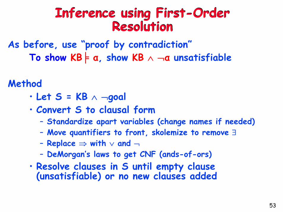
As before, use “proof by contradiction”To show KB╞ α, show KB ∧ ¬α unsatisfiable

Method• Let S = KB ∧ ¬goal• Convert S to clausal form

– Standardize apart variables (change names if needed)– Move quantifiers to front, skolemize to remove ∃– Replace ⇒ with ∨ and ¬– DeMorgan’s laws to get CNF (ands-of-ors)

• Resolve clauses in S until empty clause (unsatisfiable) or no new clauses added

54

First-Order Resolution Example

First-Order Resolution ExampleGiven

• ∀x man(x) ⇒ human(x)• ∀x woman(x) ⇒ human(x)• ∀x singer(x) ⇒ man(x) ∨ woman(x)• singer(M)

Prove• human(M)

CNF representation (list of clauses):[¬m(x),h(x)] [¬w(y), h(y)] [¬s(z),m(z),w(z)] [s(M)] [¬h(M)]

55

FOL Resolution ExampleFOL Resolution Example[¬m(x),h(x)] [¬w(y), h(y)] [¬s(z),m(z),w(z)] [s(M)] [¬h(M)]

[m(M),w(M)]

[w(M), h(M)]

[h(M)]

[]

56

Back To the Wumpus WorldBack To the Wumpus WorldRecall description:

• Squares as lists: [1,1] [3,4] etc.• Square adjacency as binary predicate.• Pits, breezes, stenches as unary predicates:

Pit(x)• Wumpus, gold, homes as functions:

Home(Wumpus)

57

Back To the Wumpus WorldBack To the Wumpus World“Squares next to pits are breezy”:

∀x, y, a, b: Pit([x, y]) ∧ Adjacent([x, y], [a, b]) ⇒Breezy([a, b])

“Breezes happen only and always next to pits”:• ∀a,b Breezy([a, b])

∃ x,y Pit([x, y]) ∧ Adjacent([x, y], [a, b])

That’s nice but these algorithms assume complete knowledge of the

world!

Hard to achieve in most cases

That’s nice but these algorithms assume complete knowledge of the

world!

Hard to achieve in most cases

Enter…Uncertainty

60

Example: Catching a flightExample: Catching a flightSuppose you have a flight at 6pmWhen should you leave for SEATAC?

• What are the traffic conditions?• How crowded is security?

61

Leaving time before 6pm P(arrive-in-time)20 min 0.0530 min 0.2545 min 0.5060 min 0.75120 min 0.981 day 0.99999

Probability Theory: Beliefs about eventsUtility theory: Representation of preferences

Decision about when to leave depends on both:Decision Theory = Probability + Utility Theory

62

What Is Probability?What Is Probability?Probability: Calculus for dealing with nondeterminism and uncertainty

Probabilistic model: Says how often we expect different things to occur

Where do the numbers for probabilities come from?• Frequentist view (numbers from experiments)• Objectivist view (numbers inherent properties of universe)• Subjectivist view (numbers denote agent’s beliefs)

63

Why Should You Care?Why Should You Care?The world is full of uncertainty

• Logic is not enough• Computers need to be able to handle uncertainty

Probability: new foundation for AI (& CS!)

Massive amounts of data around today• Statistics and CS are both about data• Statistics lets us summarize and understand it• Statistics is the basis for most learning

Statistics lets data do our work for us

64

Logic vs. ProbabilityLogic vs. Probability

Symbol: Q, R … Random variable: Q …

Boolean values: T, F Values/Domain: you specifye.g. {heads, tails}, [1,6]

State of the world: Assignment of T/F to all Q, R … Z

Atomic event: a completeassignment of values to Q… Z• Mutually exclusive• Exhaustive

Prior probability akaUnconditional prob: P(Q)Joint distribution: Prob.of every atomic event

65

Types of Random VariablesTypes of Random Variables

66

Axioms of Probability TheoryAxioms of Probability TheoryJust 3 are enough to build entire theory!

1. All probabilities between 0 and 10 ≤ P(A) ≤ 1

2. P(true) = 1 and P(false) = 03. Probability of disjunction of events is:

)()()()( BAPBPAPBAP ∧−+=∨

AB

A ∧ B

True

67

Prior and Joint ProbabilityPrior and Joint Probability

We will see later how any question can be answered by the joint distribution

0.2

sunny, rain, cloudy, snow

68

Conditional ProbabilityConditional ProbabilityConditional probabilities

e.g., P(Cavity = true | Toothache = true) = probability of cavity given toothache

Notation for conditional distributions:P(Cavity | Toothache) = 2-element vector of 2-element vectors (2 P values when Toothache is true and 2 P values when false)

If we know more, e.g., cavity is also given (i.e. Cavity = true), then we have

P(cavity | toothache, cavity) = ?

New evidence may be irrelevant, allowing simplification:P(cavity | toothache, sunny) = P(cavity | toothache) = 0.8

1

69

Conditional Probability Conditional Probability P(A | B) is the probability of A given BAssumes that B is the only info known.Defined as:

)()(

)(),()|(

BPBAP

BPBAPBAP ∧

==

A BA∧B

70

Dilemma at the Dentist’sDilemma at the Dentist’s

What is the probability of a cavity given a toothache?What is the probability of a cavity given the probe catches?

71

P(toothache) = ?

Probabilistic Inference by EnumerationProbabilistic Inference by Enumeration

P(toothache)= .108+.012+.016+.064= .20 or 20%

72

Inference by EnumerationInference by Enumeration

P(toothache∨cavity) = ? .2 + ?.108 + .012 + .072 + .008 - (.108+.012)

= .28

73

Inference by EnumerationInference by Enumeration

74

Problems with EnumerationProblems with EnumerationWorst case time: O(dn)

where d = max arity of random variables e.g., d = 2 for Boolean (T/F)

and n = number of random variablesSpace complexity also O(dn)

• Size of joint distributionProblem: Hard/impossible to estimate all O(dn) entries for large problems

75

IndependenceIndependenceA and B are independent iff:

)()|( APBAP =

)()|( BPABP =

)()(

)()|( APBP

BAPBAP =∧

=

)()()( BPAPBAP =∧

These two constraints are logically equivalent

Therefore, if A and B are independent:

76

IndependenceIndependence

Complete independence is powerful but rareWhat to do if it doesn’t hold?

4 values2 values

77

Conditional IndependenceConditional Independence

Instead of 7 entries, only need 5 (why?)

78

Conditional Independence IIConditional Independence IIP(catch | toothache, cavity) = P(catch | cavity)P(catch | toothache,¬cavity) = P(catch |¬cavity)

Why only 5 entries in table?

79

Power of Cond. IndependencePower of Cond. IndependenceOften, using conditional independence reduces the storage complexity of the joint distribution from exponential to linear!!

Conditional independence is the most basic & robust form of knowledge about uncertain environments.

80

Thomas BayesThomas Bayes

Publications:Divine Benevolence, or an Attempt to Prove That the Principal End of the Divine Providence and Government is the Happiness of His Creatures (1731)

An Introduction to the Doctrine of Fluxions(1736)

An Essay Towards Solving a Problem in the Doctrine of Chances(1764)

Reverand Thomas BayesNonconformist minister

(1702-1761)

81

Recall: Conditional Probability Recall: Conditional Probability P(x | y) is the probability of x given yAssumes that y is the only info known.Defined as:

)(),(

)(),()|(

)(),()|(

xPyxP

xPxyPxyP

yPyxPyxP

==

=

Therefore?

82

Bayes’ RuleBayes’ Rule

)()()|()(

)()|()()|(),(

yPxPxyPyxP

xPxyPyPyxPyxP

=

⇒==

What this useful for?

83

Bayes’ rule is used to Compute DiagnosticProbability from Causal Probability

Bayes’ rule is used to Compute DiagnosticProbability from Causal Probability

E.g. let M be meningitis, S be stiff neckP(M) = 0.0001, P(S) = 0.1, P(S|M)= 0.8 (note: these can be estimated from patients)

P(M|S) =

84

Normalization in Bayes’ RuleNormalization in Bayes’ Rule

)()|(1

),(1

)(1

)()|()(

)()|()(

xPxyPxyPyP

xPxyPyP

xPxyPyxP

xx∑∑

===

==

α

α

α is called the normalization constant

85

Cond. Independence and the Naïve Bayes ModelCond. Independence and the Naïve Bayes Model

86

Example 1: State EstimationExample 1: State Estimation

Suppose a robot obtains measurement zWhat is P(doorOpen|z)?

87

Causal vs. Diagnostic ReasoningCausal vs. Diagnostic Reasoning

P(open|z) is diagnostic.P(z|open) is causal.Often causal knowledge is easier to obtain.Bayes rule allows us to use causal knowledge:

)()()|()|( zP

openPopenzPzopenP =

count frequencies!

88

State Estimation ExampleState Estimation Example

P(z|open) = 0.6 P(z|¬open) = 0.3P(open) = P(¬open) = 0.5

67.032

5.03.05.06.05.06.0)|(

)()|()()|()()|()|(

==⋅+⋅

⋅=

¬¬+=

zopenP

openpopenzPopenpopenzPopenPopenzPzopenP

Measurement z raises the probability that the door is open from 0.5 to 0.67

89

Combining EvidenceCombining Evidence

Suppose our robot obtains another observation z2.

How can we integrate this new information?

More generally, how can we estimateP(x| z1...zn )?

90

Recursive Bayesian UpdatingRecursive Bayesian Updating

),,|(),,|(),,,|(),,|(

11

11111

−

−−=

nn

nnnn

zzzPzzxPzzxzPzzxP

K

KKK

Markov assumption: zn is independent of z1,...,zn-1given x.

)()|(),,|()|(

),,|(),,|()|(

),,|(),,|(),,,|(),,|(

...1...1

11

11

11

11

11111

xPxzPzzxPxzP

zzzPzzxPxzP

zzzPzzxPzzxzPzzxP

ni

in

nn

nn

nn

nn

nnnn

∏=

−

−

−

−

−−

=

=

=

=

αα K

K

K

K

KKK

Recursive!

91

Incorporating a Second Measurement Incorporating a Second Measurement

P(z2|open) = 0.5 P(z2|¬open) = 0.6

P(open|z1)=2/3 = 0.67

625.085

31

53

32

21

32

21

)|()|()|()|()|()|(),|(

1212

1212

==⋅+⋅

⋅=

¬¬+=

zopenPopenzPzopenPopenzPzopenPopenzPzzopenP

• z2 lowers the probability that the door is open.

92

These calculations seem laborious to do for each problem domain –

is there a general representation scheme for

probabilistic inference?

Yes!

93

Enter…Bayesian networksEnter…Bayesian networks

94

What are Bayesian networks?What are Bayesian networks?Simple, graphical notation for conditional independence assertions

Allows compact specification of full joint distributions

Syntax:• a set of nodes, one per random variable• a directed, acyclic graph (link ≈ "directly influences")• a conditional distribution for each node given its parents:

P (Xi | Parents (Xi))

For discrete variables, conditional distribution = conditional probability table (CPT) = distribution over Xi for each combination of parent values

95

Back at the Dentist’sBack at the Dentist’sTopology of network encodes conditional independence assertions:

Weather is independent of the other variablesToothache and Catch are conditionally independent of each other given Cavity

96

Example 2: Burglars and EarthquakesExample 2: Burglars and EarthquakesYou are at a “Done with the AI class” party.Neighbor John calls to say your home alarm has gone off (but neighbor Mary doesn't).

Sometimes your alarm is set off by minor earthquakes.

Question: Is your home being burglarized?

Variables: Burglary, Earthquake, Alarm, JohnCalls, MaryCalls

Network topology reflects "causal" knowledge:• A burglar can set the alarm off• An earthquake can set the alarm off• The alarm can cause Mary to call• The alarm can cause John to call

97

Burglars and EarthquakesBurglars and Earthquakes

98

Compact Representation of Probabilities in Bayesian Networks

Compact Representation of Probabilities in Bayesian Networks

A CPT for Boolean Xi with k Boolean parents has 2k

rows for the combinations of parent values

Each row requires one number p for Xi = true(the other number for Xi = false is just 1-p)

If each variable has no more than k parents, an n-variable network requires O(n · 2k) numbers

• This grows linearly with n vs. O(2n) for full joint distribution

For our network, 1+1+4+2+2 = 10 numbers (vs. 25-1 = 31)

99

SemanticsSemanticsFull joint distribution is defined as product of local conditional distributions:

P (X1, … ,Xn) = πi = 1 P (Xi | Parents(Xi))

e.g., P(j ∧ m ∧ a ∧ ¬b ∧ ¬e)= P (j | a) P (m | a) P (a | ¬b, ¬e) P (¬b) P (¬e)

n

100

Probabilistic Inference in BNsProbabilistic Inference in BNsThe graphical independence representation yields efficient inference schemes

We generally want to compute

• P(X|E) where E is evidence from sensory measurements etc. (known values for variables)

• Sometimes, may want to compute just P(X)One simple algorithm:

• variable elimination (VE)

101

P(B | J=true, M=true)P(B | J=true, M=true)

Earthquake Burglary

Alarm

MaryJohn

P(b|j,m) = α P(b,j,m) = α Σe,a P(b,j,m,e,a)

103

Structure of ComputationStructure of Computation

Repeated computations ⇒ use dynamic programming?

104

Variable EliminationVariable EliminationA factor is a function from some set of variables to a specific value: e.g., f(E,A,Mary)

• CPTs are factors, e.g., P(A|E,B) function of A,E,B

VE works by eliminating all variables in turn until there is a factor with only the query variable

To eliminate a variable:1. join all factors containing that variable (like

DBs/SQL), multiplying probabilities• 2. sum out the influence of the variable on new factor

P(b|j,m) = α P(b) Σe P(e) Σa P(a|b,e)P(j|a)P(m|a)

106

Other Inference AlgorithmsOther Inference AlgorithmsDirect Sampling:

• Repeat N times:– Use random number generator to generate sample values for each

node– Start with nodes with no parents– Condition on sampled parent values for other nodes

• Count frequencies of samples to get an approximation to joint distribution

Other variants: Rejection sampling, likelihood weighting, Gibbs sampling and other MCMC methods (see text)

Belief Propagation: A “message passing” algorithm for approximating P(X|evidence) for each node variable X

Variational Methods: Approximate inference using distributions that are more tractable than original ones

(see text for details)

107

SummarySummaryBayesian networks provide a natural way to represent conditional independence

Network topology + CPTs = compact representation of joint distribution

Generally easy for domain experts to constructBNs allow inference algorithms such as VE that are efficient in many cases

108

Next TimeNext TimeGuest lecture by Dieter Fox on Applications of Probabilistic Reasoning

To Do: Work on homework #2

Bayesrules!

logic, reasoning, and uncertainty - university of washington

Documents