Logic programming beyond Prolog

Maarten van Emden

joint work with Areski Nait Abdallah

Logic programming is based on Kowalski’s procedural interpre-

tation of logic. It consists of two components:

1. interpret the Horn clauses of logic as procedures

2. use Prolog as the language in which to express the procedures

We propose that (1) can be useful when the procedural language

is not Prolog.

1

Contents

1. Logic programming and “Elements of Programming”

2. Relational programming

3. Generalized Herbrand interpretations

4. Model-theoretic semantics of relational programs

5. Fixpoint semantics of relational programs

2

1. Logic programming and EOP

If verification is loosely defined as connecting a formal specifica-tion with executable code, then logic programming is a candidateverification method.

A logic program is

1. a logic formula that defines the relation (often a partial func-tion) to be computed

2. compiled to executable code.

(1) would have to play the role of the code’s specification.

3

Logic formula as specification of sortedness:

sort(X, Y) :- perm(X, Y), ordered(Y). (1)

This is also executable in Prolog.

The following shows that logic programming can do better:

sort([], []).

sort(V, W) :- split(V, V0, V1),

sort(V0, W0), sort(V1, W1),

merge(W0, W1, W).

But this is not acceptable as a specification: it is a problem-

solving recipe expressed as a logical formula.

4

“Elements of Programming” by Stepanov and McJones (2009)(hereinafter “EOP”) picks up where logic programming left off.

EOP: Specification → Theorem → C++ code

EOP Logic Programming

Spec. linear order, (1) (1)Thm. Merge sort theorem Prolog Merge sort programCode Derived C++ code ditto

According to EOP, the specification consists of logic axioms forsortedness (similar to (1)) plus the axioms for linear order. Freeof algorithmic considerations.

In EOP, the theorem is also stated in logic, and expresses thealgorithmic trick. C++ code relates to the theorem; it relatesto the axioms only via the theorem.

5

Advantages of EOP:

1. The axioms are standard, from your algebra textbook. In ad-

dition, computing suggests new concepts to be axiomatized.

2. Exploits the abstractness of logic: the axioms in the specifi-

cation are true of any structure that satisfies the axioms. I.e.

in the case of sorting not just linked lists, as in Prolog, but

any structure that satisfies the axioms for linear ordering.

3. Keeps the specification free from algorithmic considerations.

Q: What else is there to do? A: Relational Programming.

6

2. Relational Programming

Goal: to bring Theorem closer to Code while maintaining theadvantages of EOP.

Method: Modify logic programming.

1. Instead of Prolog as language for expressing procedures, someother procedural language, for example C++.

2. Instead of clauses, classical logic syntax.

3. Instead of Herbrand interpretations, F -interpretations witharbitrary universes of discourse. The model-theoretic andfixpoint semantics of logic programs transfer to relationalprograms.

7

Example

Theorem as clausal program:

sort([],[]).

sort(V, W) :- split(V,V0,V1),

sort(V0,W0), sort(V1,W1),

merge(W0,W1,W).

Theorem as relational program:

∀v, w. sort(v, w) ←(v = nil ∧ w = nil) ∨(∃v0, v1, w0, w1. split(v, v0, v1) ∧sort(v0, w0) ∧ sort(v1, w1) ∧merge(w0, w1, w)

)

8

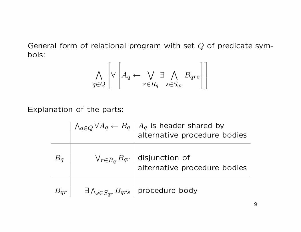
General form of relational program with set Q of predicate sym-bols:

∧q∈Q

∀Aq ← ∨

r∈Rq∃

∧s∈Sqr

Bqrs

Explanation of the parts:∧q∈Q ∀Aq ← Bq Aq is header shared by

alternative procedure bodies

Bq∨r∈Rq Bqr disjunction of

alternative procedure bodies

Bqr ∃∧s∈Sqr Bqrs procedure body

9

3. Generalizing Herbrand interpretations

F -interpretation: fix domain of discourse D and fix interpretationF for the function symbols. F -interpretations only differ in theirinterpretation of the predicate symbols and can be viewed asvectors of relations over D indexed by predicate symbols.

Partial order: element-wise set-theoretic inclusion.

Possible F -interpretation: D is Herbrand universe, F maps f tothe function that maps (t0, . . . , t|q|−1) to (the symbolic term)f(t0, . . . , t|q|−1).

A more typical F -interpretation might have D consisting of thenatural numbers with fixed interpretations (the usual ones) for 0,1, +, and ×. This would be an F -model of the semiring axioms.

10

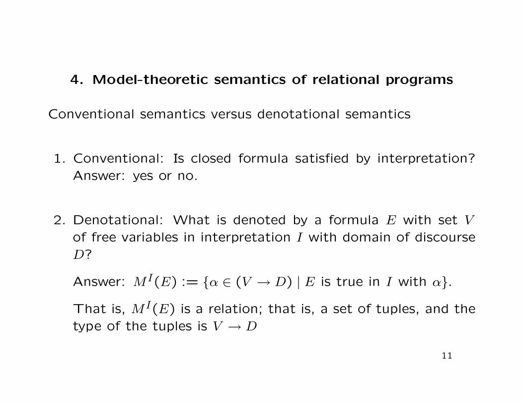
4. Model-theoretic semantics of relational programs

Conventional semantics versus denotational semantics

1. Conventional: Is closed formula satisfied by interpretation?Answer: yes or no.

2. Denotational: What is denoted by a formula E with set V

of free variables in interpretation I with domain of discourseD?

Answer: MI(E) := {α ∈ (V → D) | E is true in I with α}.

That is, MI(E) is a relation; that is, a set of tuples, and thetype of the tuples is V → D

11

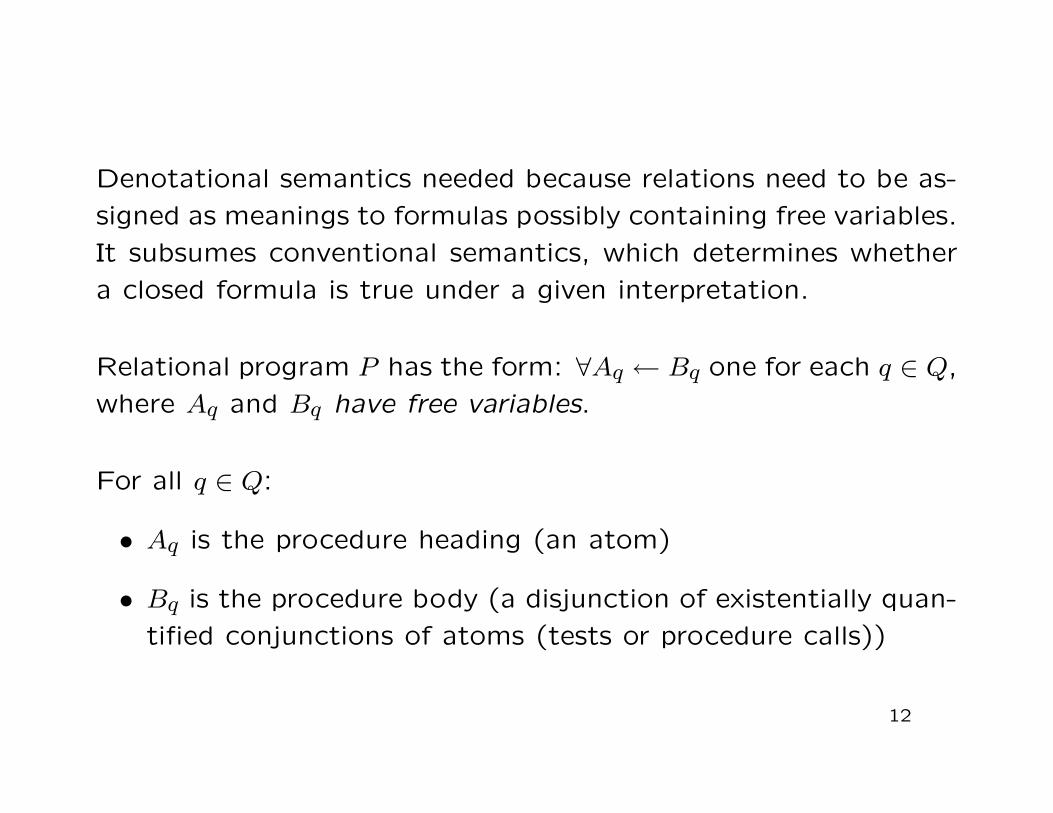
Denotational semantics needed because relations need to be as-

signed as meanings to formulas possibly containing free variables.

It subsumes conventional semantics, which determines whether

a closed formula is true under a given interpretation.

Relational program P has the form: ∀Aq ← Bq one for each q ∈ Q,

where Aq and Bq have free variables.

For all q ∈ Q:

• Aq is the procedure heading (an atom)

• Bq is the procedure body (a disjunction of existentially quan-

tified conjunctions of atoms (tests or procedure calls))

12

Given a relational program P with set Q of predicate symbols

and an F -interpretation I with domain D.

For all q ∈ Q we have that MI(Aq) and MI(Bq) are relations of

type Vq → D, where Vq is the set of free variables of Aq and Bq.

Definition: An F -interpretation I is a model of P iff

MI(Aq) ⊇MI(Bq)

for all q ∈ Q.

Theorem: P has a least model.

Proof: The intersection of any non-empty set of models of P is

a model of P .13

5. Fixpoint semantics

int f(int n) { if (n == 0) return 1; return n*f(n-1); }

n 0 1 2 3 4 . . .⊥ ⊥ ⊥ ⊥ ⊥ ⊥ . . .

Tf(⊥) 1 ⊥ ⊥ ⊥ ⊥ . . .

T2f (⊥) 1 1 ⊥ ⊥ ⊥ . . .

T3f (⊥) 1 1 2 ⊥ ⊥ . . .

T4f (⊥) 1 1 2 6 ⊥ . . .

The function f computes limn→∞ Tnf (⊥).

This limit is the least fixpoint of Tf :

Tf( limn→∞T

nf (⊥)) = lim

n→∞Tnf (⊥)

.14

In Scott’s fixpoint semantics, the mapping TP of type

(N ↪→ N )→ (N ↪→ N )

is computed by the body of the recursively defined program func-

tion and acts on partial functions of type N ↪→ N .

In logic programming, recursively defined procedures compute

relations, of which partial functions are a special case. TP maps

relations to relations. The mapping is defined by the bodies of

recursively defined procedures. The q-th procedure has the form

Aq ← Bq.

The body defines the relation MI(Bq). TP is defined as the

mapping from I to an interpretation that has MI(Bq) as its q-th

component.

15

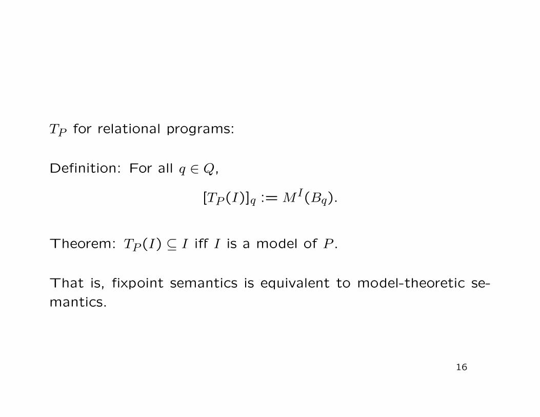
TP for relational programs:

Definition: For all q ∈ Q,

[TP (I)]q := MI(Bq).

Theorem: TP (I) ⊆ I iff I is a model of P .

That is, fixpoint semantics is equivalent to model-theoretic se-

mantics.

16

TP for relational programs:

Definition: For all q ∈ Q,

[TP (I)]q := {~d ∈ D|q| | Bq is true in I with ~d ◦ (~x)−1}

where ~d is (d0, . . . , d|q|−1), ~x is (x0, . . . , x|q|−1), ◦ is function com-

position, and ~x has an inverse because no repeated occurrence

of any of the variables.

Think of it as [TP (I)]q := λ(x0, . . . , x|q|−1).MI(Bq).

Theorem: TP (I) ⊆ I iff I is a model of P .

That is, fixpoint semantics is equivalent to model-theoretic se-

mantics.17

7. Future work

1. Transcription of relational programs to C++ is easy enough.However, those who are oppressed by the size and complexityof C++ might be interested in the language resulting fromeliminating everything not needed for the transcription ofrelational programs.

2. Conversely, formal logic was formed a century ago and has,with few exceptions, only been used for theoretical purposes.Even textbooks on abstract algebra give the axioms infor-mally. Logic lacks facilities for writing large formulas in astructured fashion. It may benefit from structuring facilitiesinvented for conventional programming languages.

18

8. Conclusions

1. Fixpoint and model-theoretic semantics of logic programs

with respect to Herbrand interpretations generalize to these

semantics for relational programs with respect to F -interpretations.

2. Kowalski’s Procedural Interpretation of Logic, has not only

procedurally interpreted Horn clauses, but also limited the

language for expressing procedures to pure Prolog. This

work does interpret Horn clauses as procedures, but leaves

open the choice of procedural language.

3. We do not propose to replace Prolog, but to expand the

scope of logic programming.

19

Appendix: Hierarchical relational programs

The set of clauses of a relational program can be decomposedinto mutually disjoint recursion clusters. Each of these may im-port predicates from other clusters. Clusters are partially orderedaccording to whether one imports from another.

The results obtained above hold for each cluster as a separaterelational program where there is a distinction between importedpredicates, which do not occur in a left-hand side and those thatdo.

Henceforth consider only relational programs that do not de-compose into recursion clusters. For these it does not matterwhether the imported predicates are defined by another relationalprogram: they could be defined by a textbook structure.

20

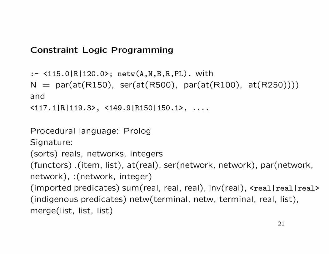
Constraint Logic Programming

:- <115.0|R|120.0>; netw(A,N,B,R,PL). with

N = par(at(R150), ser(at(R500), par(at(R100), at(R250))))

and

<117.1|R|119.3>, <149.9|R150|150.1>, ....

Procedural language: Prolog

Signature:

(sorts) reals, networks, integers

(functors) .(item, list), at(real), ser(network, network), par(network,

network), :(network, integer)

(imported predicates) sum(real, real, real), inv(real), <real|real|real>

(indigenous predicates) netw(terminal, netw, terminal, real, list),

merge(list, list, list)

21

netw(A,at(R),B,R,(r150:1).nil) :- <149.9|R|150.1>;.

% Similarly for 100, 250, and 500 ohms.

netw(A,ser(N1,N2),C,R,PL)

:- sum(R1,R2,R);

netw(A,N1,B,R1,PL1), netw(B,N2,C,R2,PL2),

merge(PL1,PL2,PL).

netw(A,par(N1,N2),B,R,PL)

:- inv(R,RR),inv(R1,RR1),inv(R2,RR2), sum(RR1,RR2,RR);

netw(A,N1,B,R1,PL1), netw(A,N2,B,R2,PL2),

merge(PL1,PL2,PL).

22