logic-based representation and reasoning about knowledge of constrained resources

E L S E V I E R Knowledge-Based Systems 10 (1997) 71-80

KnowledcJe-Ba~d 5 V S T E M $ - ' - -

Logic-based representation and reasoning about knowledge of constrained resources

Y o u n g U . R y u

Department of Decision Sciences, The University of Texas at Dallas, P.O. Box 830688, M/S JO 4.4, Richardson, Texas 75083-0688, USA

Received 19 June 1996; accepted 2 October 1996

Abstract

It appears that classical logic is not suitable for the representation and reasoning about knowledge of disposable resources. The major difference between reasoning about disposable resources and classical logic is that once a disposable resource is used to produce something, it is not available any more; but a formula of classical logic can be repeatedly used in deduction. Inspired by linear logic, or logic of resources, we propose a language for knowledge-based systems of resources, which can process state space models of systems represented by Petri nets or their subclasses such as marked graphs and state machines. It can serve as a modeling tool for various engineering and social science problems of resource allocations.

Keywords: Constrained resource programming; Constraint logic programming; Logic-based knowledge representation: Petri nets

1. Introduction

Processing data of constrained resources is a pervasive practice in engineering and social sciences. Low-level data processing of electronic computers is often viewed as resource processing at the abstract representation [1]. Production scheduling can be understood as decision making for an asset maximization with transformation of scarce resources [2]. Commodity-market equilibra- tion can be understood as the processing and allocation of resources with various constraints on prices and markets [3]. This paper is concerned with logic-based knowledge representation and reasoning about such constrained resource problems.

Logic is a language for abstract representations of concepts/objects and their relationships [4] as well as a declarative programming language [5]. It is especially useful in the representation of qualitative conditions [6] and often recommended as a paradigm to integrate mathematical programming with heuristic processing of nonnumeric constraints [7]. The weakness of numeric processing of data in logic is recently complemented by a constraint reasoning extension to logic programming, called the constraint logic programming scheme [8].

lnternet: [email protected] WWW: http://wwwpub.utdallas.eduN ryoung

0950-7051/97/$17.00 © 1997 Elsevier Science B.V. All rights reserved PII: S0950-7051 (96)01057-X

Despite its expressiveness, however, there is a short- coming in classical logic when it is applied to the modeling of constrained resources.

The deduction of classical logic is not destructive and constructive. That is, the deduction of '~ ' from '4; and '~ ~ ~' does not destroy (or invalidate) 'E . How- ever, suppose we have resource 'E and a machine that transforms 'E to '~' . Then, the production --- construction, establishment, or creation of '~ ' is done by destroying 'E . As the result, '0 ' is not available any more. This notion of resource construction/destruction is addressed by recently developed non-standard logic called linear logic.

Linear logic is an known as a "resource conscious logic" [9,10] developed by extending classical and intui- tionistic logic. It provides mechanisms to destroy and construct formulas in the course of theorem proving. The analogy between linear logic theorem proving and resource construction/destruction provides a foundation for logic-based modeling of disposable resources and their consumptions. We borrow ideas of resource representation from linear logic and propose a logic-based system of resource-oriented modeling. In order to improve the constraint handling capability, we adopt a constraint satisfaction scheme in the logic programming paradigm [8,11,12]. The resulting system will be called constrained resource programming.

72 Y.U. Ryu/ Knowledge-Based Systems 10 (1997) 71 80

We will address constrained resource programming and its application as follows. Section 2 addresses the representation of knowledge of constrained resources and a reasoning scheme. The computational model is presented based on constraint logic programming paradigm. In Section 3, we propose constrained resource programming as a representation and processing language for Petri nets, which are used as a conceptual modeling tool for an application presented in Section 4. The modeling examples demonstrated in Section 4 are (1) multilateral trade matching in a sealed bid commodity auction market, whose main emphasis is placed on optimal resource allocations between traders and (2) resource requirement planning for a production system.

are producible by consuming ~1 (but not consuming ~2).

~1, ~2 +- 61, @02

means that if 02 is producible (with other machines and resources) then ~bl and ~2 are producible by consuming Ol (but not producing and consuming ~2).

means that if 4~2 is not immediately available then ~l and ~2 are producible by consuming ~1. Finally,

~ , ~ ~ ~ , ~ ~

means that if 4~2 is not producible (with other machines and resources) then ~ and ~2 are producible by consuming ~1.

2. Constrained resource programming

2.1. Representation of resources

In classical logic, if a formula is given to be true, it stays true whether or not it is used to prove other formulas. In the logic of resource, on the other hand, if a formula representing a resource is given to be available, it is not available again once it is used, or consumed, to prove, or produce, other formulas. This is the starting point of constrained resource programming.

There are two types of implication formulas. The first one

~l,~22,...,~Dn +-- ~l ,q~2,-",q~rn{¢l,~2, '" ,~k)

is understood as a durable machine that produces ~Pl, ~ 2 , . . . , and %, by consuming exactly ~bl,q~2,..., and ~,, if constraints ~1,~2,-.-, and ~k are satisfied. Note that commas at the left-hand and right-hand sides of an implication formula are considered as the commuta- tive conjunction connective. Also, we assume that all variables in formulas are universally quantified. The second type of implication formulas:

is understood as a disposable machine, functioning like a durable machine, except that it can be used only once in the deduction or production. The availability of a disposable resource is represented as an atomic formula. With a modal operator '!' denoting the unlimited availability, one can express a durable resource.

In addition to operator '!' for the unlimited availability of resources, available are a number of resource checking operators 'i', '@', '~ ' , and '-~', which are for the availability, producibility, unavailability, and unproducibility of resources, respectively. For instance,

~1,~2~---~1,i~2

means that if t~2 is immediately available then ~Pl and ~b 2

2.2. Interpreter

A constrained resource program is a bag l of two types of clauses:

(label) : (head) o- (body) { (constraints) }

{label): (head) +- {body){(constraints)},

where the optional (label) is a string identifying a formula, and (head) is conjunction of atomic predicate expressions or those prefixed by modal operator '!' and (body) is conjunction of atomic predicate expressions or those prefixed by modal operator '!', 'i', '@', '~ ' , or '~'. When there are no constraints, we omit the pair of curly braces. For an atomic formula 4~, let ~ denote either q~ or !~; similarly, let ~ denote either ~b, !~, i4~, @~, ~ , or -~b. Clause with the empty body:

~ o-- C~

where C is a set of constraints, is abbreviated as '~C' . Similarly, expression:

~ C

is abbreviated as 'bpC'. A query for ~1, ~ 2 , . . . , ~, with constraints {1, {2 , . . . , {k is expressed as:

which can be intuitively read "Are ~l, ~2 , . - . , and ~, producible under the constraints of ~l, ~2, . . - , and ~k?"

A proof state in resource programming is:

: (e , z , L)

where P is a bag of formulas, ~b i i s an atomic formula for each i, E is a set of constraints, and L is a set of pairs of a

clause and an atomic formula. From state or, a transformed state a ' is obtained by one of the following state transformation rules.

J A bag is a collection of unordered elements in which multiple occur- rent of the same element counts. For a bag B, the number of occurrence ofits¢ element a is denoted by #(a, B). We use the pair of braces '],' and ' | ' to explicitly specify a bag.

Y.U. Ryu/Knowledge-Based Systems 10 (1997) 71-80

Transformation Rule 1. When ~i = ~bi or !~b i. Select

c = 5q,f f2 , . . . ,5 'k *--- ~ l , - . . , ~ , C E P

where C U { ~ , - - ~ j } is satisfiable for some j and (c, "~j) ~ L. And then, establish a substate:

73

not exist "~ ~- C E P or ? o-- C E P such that E U C tO {~& = 3'} is satisfiable, then t r ans fo rm a to:

dr ' : ( P , ( ~ , , . . . , ~ ,,~,+, . . . . . ~ ) , Z , L ) . •

r : { (P, ( ! +1 , . - . , !On), C to {~Yi : 3"j}, L U {(e, @j)})

(P, ((~1 . . . . , ~n), C U {~ i = 3'j}, L to {(e, @j)})

i f @i = [2/3i and "~j = 7j

otherwise.

Or select

e : 3 " 1 , 3 ' 2 , ' ' ' , ' 7 k ° - - ~ l , ' ' ' , ~ n E P

where C U {~b i = 3"j} is satisfiable for s o m e j . And then, establish a substate:

~ Transformation Rule 5. When ~,~ = ~'Oi. Establish a substate:

~- = (P, ( e , ) , 0, L)

(P - {c} , ( !O l , . - . , !0,), C U {~bi = 3"j}, L) i f t~i = !~)i and ~j = 3'j

r = (P - {c}, ( ~ l , . . . , ~n), C U {~bi = 3'j}, L) otherwise.

I f r is t r ans fo rmed to: g ?

~- = ( e ' , ( ) , c ,C')

and E U C ' is satisfiable, then t r ans fo rm dr to:

dr' = (O, (d~,,... , ~ , - , , d5i+1 . . . , d~m), E tO C',L) where

I f r is not conver ted to

~ - ' = (P ' , ( ) , Z ' , L')

where z U .q' is satisfiable, then t r ans form cr to:

O" : ( P , ( ~ I , " " ' , 2 ~ i 1 ,2~i+1, • . . , ~ r n ) , - ~ , t ) • •

Given a resource p r o g r a m P0 and a query for a list o f

P'U{51C' , . . . ~kC'} i f ~ i = !~Pi or-yj = !'~j

Q = P ' u {~1C',... ~/j IC' ,~j+IC', . . . ,SkC'} otherwise. •

Transformation Rule 2. When ~i = ig)i. I f there exists ? ~ C E P or f r o - C E P such that Eto Cto {~i = h'} is satisfiable, then t r ans fo rm dr to:

drt : (P, (~1 . . . . ,~i_l,~i+l,...,~-)m),

Zto CU{t~i : 3"},L). •

Transformation Rule 3. When ~i = @~bi. Establ ish a substate:

T : ( e , (~3/)0, L )

I f "r is conver ted to

~ - ' = (~", ( ) ,S ' , C')

and E U E ' is satisfiable, then t r ans fo rm dr to:

dr'= (P,(~l,...,~bi_l,~i+l,...,~bm),EUZt,L). •

Transformation Rule 4. When ~i = "a~)i. I f there does

a tomic formulas tI, with constra ints C, if:

dro = (Po, ,~, c , O)

is t r ans fo rmed to:

o = (P,() ,~,L>,

then we say the p r o o f of • succeeds. The success of the p r o o f o f • means tha t • is producible f rom P0 by using resources of P0 - / 5 .

So far, resource p r o g r a m m i n g allows simple resource expressions at the lef t -hand and r ight -hand side o f a clause. However , by al lowing ,--- and o - expressions at the lef t-hand side o f a clause, we can increase the expressiveness o f const ra ined resource p rog ramming . Fo r instance,

~, (0' +-- ~') o-- ~

means tha t if we consume ~b then we can have (or buy or produce) resource 0 and machine 0 ' ~ 0 ' . For state

dr : (~, (~,, ~> . . . , ~ ) , e , L ) ,

we define an addi t ional t r ans fo rma t ion rule.

74 Y.U. Ryu/Knowledge-Based Systems 10 (1997) 71-80

P3 t2

t3 '7

P2

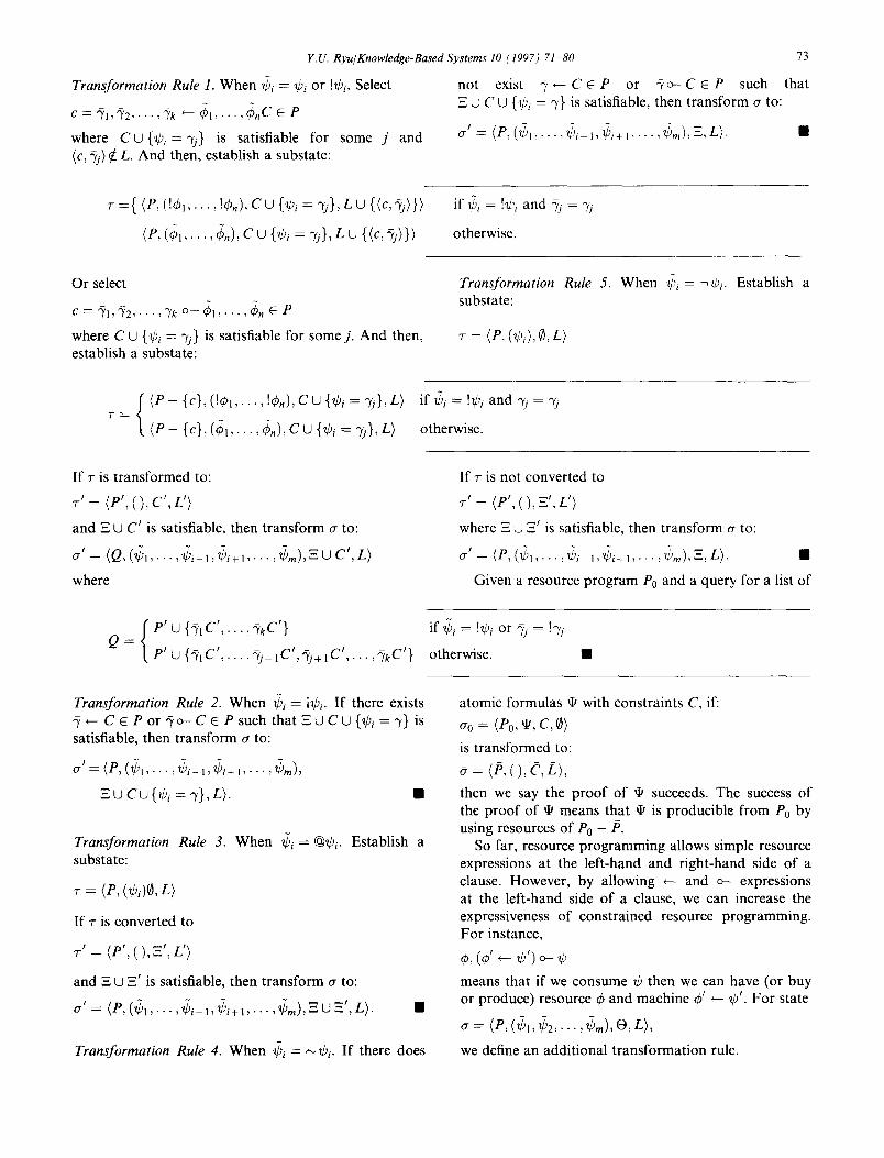
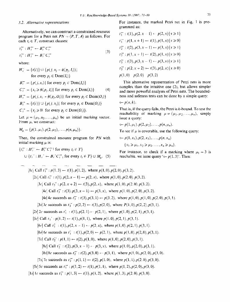
Fig. 1. A marked Petri net. Circles are place nodes, bars are transition nodes, and bullets are tokens. The weight of an arc is represented by its multiple occurrence between a place node and a transition node.

Transformation Rule 6. For ~i, if there exists clause c E P whose left-hand side contains

'~1, " T 2 , - ' ' , "~k +-- ~1, ~ 2 , " - " , q~n

o r

' ~ l , " / 2 , ' ' ' , ' ~ k o--- ~1, q ~ 2 , ' ' ' , ~n

such that {~bt = 3'j} is satisfiable for some j , then establish a substate:

net with tokens in places. A marking -- or a token placement - - is defined as a vector:

# = ( # l , # 2 , ' ' ' , ] Z n ) ,

where #i/> 0 represents the number of tokens residing in place Pi E P.

Suppose a Petri net P N = (P, T, A) with a marking # is given where IPI = n. For ti E T, let Ii be a bag over Dom(Ii) C_ p such that Dom(Ii) = {pal for every & E P such that (pj, ti, W) E A} and for every (&, ti, W) E A, #(&,Ii) = w; similarly, let Oi be a bag over Dom(O/) c_ p such that Dom(Oi) = {pj[ for every& E P such that (ti,Pj, W ) E A} and for every (ti,Pi, w ) c A, #(pj, Oi) = w. For marking # = (#1 ,#2 , . . . ,#n), let M u be a bag over Dom(Mu) C_ P such that Dom(M~) = {pj[ for every #j > 0} and #(pj, M u = #j. Then, we establish a constrained resource program for P N as follows:

k ) t i : Oi+--- Ill f o r a l l t i ~ T S u M ~. (2)

(P, (right-hand side of c), C, {(c, ~i)}) if c is a ~- clause

r = (P - {c}, (right-hand side of c), C, O) if c is a o- clause.

If it is transformed to:

~- '= (P' , (), Z', L'),

then transform a to: !

a = (Q, ( ~ , ~ 2 , . . . , ~ m ) , E , L ) ,

where

Q = P u Cleft-hand side of eE'}

3. Petri net modeling

3.1. Simple representations

A Petri net [13] is a bipartite directed multigraph, which consists of two types of nodes, called places and transitions, and directed arcs connecting a node of one type to a node of the other type. We define a Petri net as a triple:

P N = (P, T, A), (1)

where P is a set of places, T is a set of transitions, and A is a set of weighted directed arcs defined as:

A = { ( p , t , w ) [ p E P , t E T,w E Z}

x U{(t ,p ,w)[t E T ,p E P ,w E Z},

where Z is the set of non-negative integers. For a = ( p , t , w ) E A or a = (t,p,w) EA, w is called the weight of a. Say [PI -- n. A marked Petri net is a Petri

A place is specifically identified by a unique constant as the first argument of a special predicate symbol 'p'. For instance, the marked Petri net in Fig. 1 is represented as:

t 1 : p ( 1 ) e-- p(2)

t 2 :p(1) +-p(3)

t3: p(2),p(2) +--- p(3)

p(3) p(3)

The constrained resource programming interpreter can perform various analyses for Petri nets. Suppose a program for a marked Petri net is constructed. The boundedness and the safeness of the Petri net are tested as follows. If the query of:

times

o- ,p(x;

fails, then the Petri net is k-bounded. If it fails when k -- 2, then the Petri net is safe. The boundedness and the safeness tests are special cases of the coverability problem. Say ~o is a bag of places corresponding to a marking #. The success or failure of the query 'o- ~ ' solves the coverability problem of #. That is, if the query 'o-- ~ ' succeeds, then there is a reachable marking

! # such that #'~> #. A restricted form of the coverability problem, called the reachability problem, is addressed as follows. If the query ' o - ko' succeeds, but ' o - - ~ U ) p ( x ) f ' fails, then the marking represented by • is reachable.

'K L

Y.U. Ryu/Knowledge-Based Systems 10 (1997) 71 80

3.2. Alternative representations

Alternatively, we can construct a constrained resource program for a Petri net PN = (P, T, A) as follows. For each t i G T, construct clauses:

tT- : 1-17- ~- B 7 - C 7 {3)

t 7 : H E ~- B E C y

where:

H E = {t(i)} U {p(j , xj - #(pj, I,)) [

for every & ¢ Dom(I/)}

B~ 7 = {p(j , xi)] for every p j ¢ Dom(Ii)}

C 7 = {xj >>. #(&, Ii)l for every & ¢ Dom(I;)} (4)

H 7 = {p(j , x / + #(pj, Oi))1 for every pj E Dom(Oi)}

B y = {t(i)} U {p(j , xi) [ for every pj E Dom(Oi)}

C 7 = {x i >/0[ for every p, e Dom(Oi)}.

Let # = (#1,u2 . . . . ,# , ) be an initial marking vector. From #, we construct:

M u = {p(1,/zl),p(2, #2), .-- ,p(n, #,)}.

Then, the constrained resource program for PN with initial marking > is:

{t~7 : HT- ~- BvCT-I for every t i E T}

U { t , : H y ~ B7~C71 for every t i e T} U M u. (5)

For instance, the marked grammed as:

tl-

t7 t7

t;-

tV

p(1

Petri net in

: t(1),p(2, x - 1) ~p(2 , x ) {x>~ l}

: p(1,x + 1) ~-- t(1) ,p(1,x){x >~ 0}

: t ( Z ) , p ( 3 , x - 1) ~--p(3, x){x>~ 1}

: p ( 1 , x + 1 ) ~ t(Z),p(1,x){x>~O}

: t ( 3 ) , p ( 3 , x - 1) ~--p(3 ,x ){x~ 1}

: p(2, x + 2) +-- t(3),p(Z,x){x >>. 0}

,0) p(2, O) p(3,2)

75

Fig. 1 is pro-

This alternative representation of Petri nets is more complex than the intuitive one (2), but allows simpler and more powerful analyses of Petri nets. The bounded- hess and safeness tests can be done by a simple query:

o- p(x, k).

That is, if the query fails, the Petri is k-bound. To test the reachability of marking # = (/x1,#2, . . . ,#, , ) , simply issue a query:

o- p(1,/~l),P(2, #2) . . . . ,p(n, Iz~).

To see if # is eoverable, use the following query:

o--- p(1, Xl ),p(2, x2) , . . . ,p(n, x ,)

{Xl ~ #I ,X2 ~ t1'2 . . . . ,Xn ~ ]In}.

For instance, to check if a marking where Izl = 3 is reachable, we issue query 'o-- p(1,3)' . Then:

[lc] Call tT': p(1,3) +- t(1),p(1,2), where p(1,0) ,p(2,0) ,p(3, 2).

[2c] Call t i - : t ( 1 ) , p ( Z , x - 1)*-- p(Z,x), where p(1,O),p(Z,O),p(3,2).

[3c] Call t3+: p(2, x + 2) ~ t(3),p(2, x), where p(1,0),p(2, 0),p(3, 2).

[4c] Call t~-: t ( 3 ) , p ( 3 , x - 1) ~--p(3, x), where p(1,O),p(Z,O),p(3,2).

[4s] 4c succeeds as t~-: t(3),p(3, 1) +- p(3,2), where p(1,O),p(1,O),p(Z,O),p(3, 1).

[3s]3e succeeds as t3' :p(2,2) ~ t(3),p(2,0), where P(1,O),p(Z,2),p(3, 1).

[2s] 2e succeeds as t ~ : t(1), p(2, 1) ~ p(2, 1 ), where p(1,0), p(2, 1 ), p(3, 1).

[5c] Call t~ :p(1,2) +--- t(1),p(1, 1), where p(1,0),p(2, 1),p(3, 1).

[6c] Call t]- : t ( l ) , p ( 2 , x - 1 ) ~-- p(2,x), where p(1,0),p(2, 1),p(3, 1).

[6s] 6c succeeds as t~ : t(1),p(2,0) +-p(2, 1), where p(1,O),p(2,0),p(3, 1).

[7c] Call t ~ : p(1, 1 ) ~ t(2),p(1,0), where p(1,O),p(2,0),p(3, 1).

[8c] Call t~- : t(Z),p(3, x - 1) ~ p(3, x), where p(1,0),p(2, 0),p(3, 1).

[8s] 8c succeeds as t~- : t(2),p(3, 0) ~ p(3, 1), where p(1,0),p(2, 0),p(3,0).

[7s] 7c succeeds as t { : p(1, 1) ~ t(Z),p(1,0), where p(1, 1),p(2, 0),p(3,0).

[5s] 5e succeeds as t~' : p(1,2) ~ t( l) ,p(1, 1), where p(1,2),p(Z,O),p(3,0).

[ls] lc succeeds as tT" : p(1,3) +- t(1),p(1,2), where p(l , 3),p(2, 0),p(3, 0).

76 Y.U. Ryu/Knowledge-Based Systems 10 (1997) 7l 80

That is, the query 'o--p(1,3) ' succeeds by firing transitions in the sequence of t3, tl, tl, and t2.

3.3. Coloring

Consider a variation of Petri nets (1) with the following extensions:

• A number of attributes are assigned to each place. We represent such a place with n attributes as pj(yj, x]), where Y1 is a vector of n terms such that each term Yj,l ranges over a certain domain A],t and xj ranges over the set of real numbers ]~ denoting the number of tokens.

• The weight of an arc is defined as a function on attributes of the place connected to the arc. That is, an arc is represented a s (pj(yj, xj) , t i , f (yj) ) or (ti,Pj(yj, x j ) , f (y j )) . The co-domain of weight func- tions is ~.

• Additional constraints are associated with each transition. Let ei be the additional constraints of transition ti.

• In order for a transition to fire, (i) the number of tokens in every input place must be greater than or equal to the weight of the arc connecting from the place to the transition and (ii) the additional constraints of the transition must be satisfied. When the transition fires, the number of tokens removed from an input place is the value of the weight function of the arc connecting from the input place to the transition. After a transition is fired, the number of tokens created in an output place is the value of the weight function of the arc connecting from the transition to the output place.

This extended Petri net is often called a colored Petri net.

In order to represent the extended Petri net, we modify (4) as follows:

/47-=-

B7---

C7-=

H ~ ' =

B ~ =

{tCi, Y~, Zi)} U {p(j , yj, xj -fjCYj)) I

for every p] ~ Dom(Ii)}

{p(j , yj, xj)r for every pj E Dom(li)}

{xj >_-fj(yj)] for every pj ~ Dora(I/)} (6)

{p(j , zk, xk + gk(zk))[ for every Pk E Dom(Oi)}

{t(i, Yi, Zi)} t..J {PCj, zk, Xk)I for every Pk E Dom(Oi)}

{xk i> 01 for every pk 6 Dom(Oi)} U el, c 7 =

where Yi is the list o fy j for allpj E Dom(Ii) and Zi is the list Of Zk for all Pk E Dom(Oi). n tokens residing in place pj are represented as p(j , ~j, n); other m tokens residing in the same place, but a different color specified by ~.j, are represented as p(j ,~j ,m). These two sets of tokens,

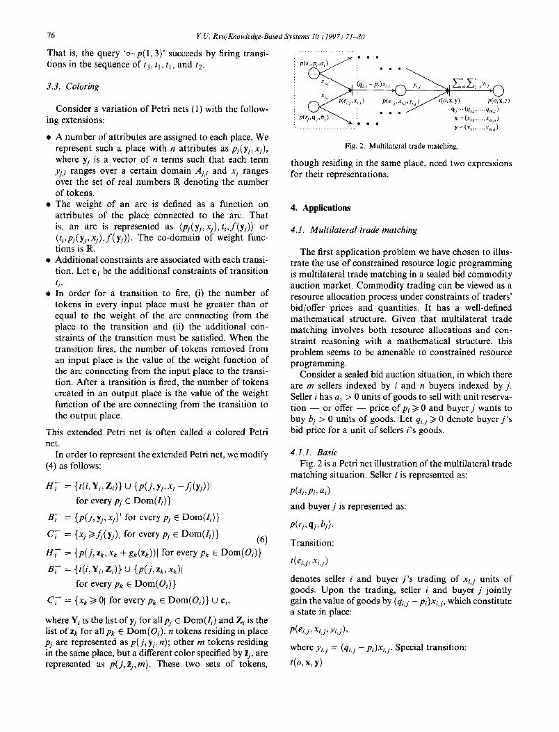
P(si,p~,ai) f • • • •

f . ~ ' J t ( e , . j , x , , i ) p(%,x, . j ,y ,4)~./ f t(o,x,y) p(o,x,z) , k - - - ~ . . ~ i . . . ~ q j =(qt4 ..... q~,j)

p(rj,qj,bj) ~ :e . . x=(x l , t ..... x~..)

. . . . . . . . . . . . . . . . . . . . " Y = (YH ..... Y~.. )

Fig . 2. M u l t i l a t e r a l t r a d e m a t c h i n g .

though residing in the same place, need two expressions for their representations.

4. Appficafions

4.1. Multilateral trade matching

The first application problem we have chosen to illus- trate the use of constrained resource logic programming is multilateral trade matching in a sealed bid commodity auction market. Commodity trading can be viewed as a resource allocation process under constraints of traders' bid/offer prices and quantities. It has a well-defined mathematical structure. Given that multilateral trade matching involves both resource allocations and constraint reasoning with a mathematical structure, this problem seems to be amenable to constrained resource programming.

Consider a sealed bid auction situation, in which there are m sellers indexed by i and n buyers indexed by j. Seller i has a i > 0 units of goods to sell with unit reserva- tion - - or offer - - price of Pi >~ 0 and buyer j wants to buy bj > 0 units of goods. Let qi,j ~ 0 denote buyer j ' s bid price for a unit of sellers i's goods.

4.1.1. Basic Fig. 2 is a Petri net illustration of the multilateral trade

matching situation. Seller i is represented as:

p(Si ,Pi , ai)

and buye r j is represented as:

p(rj,qj, bj).

Transition:

t (e i , j , x i , j )

denotes seller i and buyer j ' s trading of xi, j units of goods. Upon the trading, seller i and buyer j jointly gain the value of goods by (qi,j - p i )x i , j , which constitute a state in place:

p(ei , j , xi , j , Yi, j) ,

w h e r e Yi,j = (qi,j - p i )x i , j • Special t r a n s i t i o n :

t(o, x, y)

Y.U. Ryu/Knowledge-Based Systems 10 (1997) 71-80

• 7 • • ID

• p'(s~,u,,x~) t'(s,,u~) J

y' -b: , i

v = ( v t ..... v ) * p'(rj,vj,yj) t'(r),vj) ~=~x, ..... ~) .. ............ .-.....?...% y=(y j ..... y.)

Fig. 3. A dua l r e p r e s e n t a t i o n o f mu l t i l a t e r a l t r a d e m a t c h i n g .

aggregates trading gains achieved by all sellers and buyers' trading activities so that the final state

p(o, x, z)

is established. Fig. 2 is represented as the following constrained

resource program:

to :p , x , z + Yi, ~ - - t ( o , x , y ) , p ( o , x , z ) { x > ~ O }

t ~ : t (o ,x , y ) ,p ( r l , l ,X l , l ,O) , . . . , p ( rm,n ,Xm,n ,O)

P( r s ,1, x1,1, Y 1 , 1 ) , - . . , p( rm,n, Xm,n, Ym,n)

t ~ : p(ri,j, xi,s, Yi,j + (qi,j - pi)xi,j)

~-- t(ri,j),p(ri, j, xi,j, Yi,j)

t~i. j : t(ri,j, xi , j ) ,p(si ,Pi , a i - xi , j ) ,p(rj , qj, bj - xi,j)

+-- P(si,pi, ai),p(rj, q j, bj)

p(si,Pi, ai) p(r j ,q j , bj) p(ri , j ,xi , j ,O ) p(o,x, 0)

In response to query 'c~-p(o, x m a x - l ( z ) ) ', the constrained resource programming interpreter solves:

m n

z = max Z E ( q i , J - Pi)Xi,j (7) i - I j-I

~-~Xi, j ~ a i for i = 1 . . . . , m j = l

~ _ _ X i , j ~ b j for j = 1 , . . . , n i = 1

Xi, j ) 0 for i = 1 , . . . , m and j = 1 , . . . , n .

(max-m denotes the inverse function of max.)

(7a)

(7b)

4.1.2. A dual representation For a given Petri net, its dual is obtained by reversing

the direction of arcs and interchanging place nodes and transition nodes. The nucleus of the multilateral trade matching representation in Fig. 2 consists of place nodes of sellers and buyers and transition nodes of their tradings, as showed in the dotted round rectangle. Its dual is constructed in such a way that (i) the place node corresponding to t(ei,j, xi,j) is represented as

77

Pt(ei,j, q i , j - -Pi) , where q i , j - - P i is the output ratio of t(ei,j, xi,j), (ii) the transition node corresponding to P(si,pi, ai) is t'(si, ui) where all input arcs have a weight of ui and the output arc has a weight of -a~ui, and (iii) the transition node corresponding to p(r j ,q j , bj) is / ( r j , vj) where all input arcs have a weight of vj and the output arc has a weight of -b jv j . It is illustrated in the dotted round rectangle in Fig. 3, together with other transition and place nodes that aggregate tokens -aiu~ and - b j vj.

The following is a constrained resource program of Fig. 3:

t ~ : p ' ( o , u , v , w + xi-~- y j ) i= 1 j = l

~-- t ' ( o , u , v , x , y ) , p ' ( o , u , v , w ) { u > ~ O , v > ~ O }

t o''- : t ' ( o , u , v , x , y ) , p ' ( s l ul,O),.. ' , . , p (Sin, Urn, O),

p'(rl , vl, 0) , . . . ,p'(rn, vn, 0)

*-- P'(Sl , Ul, Xl ) , . . . ,p'(Sm, Um, Xm), p ' (r l , zq, Yl ), - - •,

P'(rn,vn,yn)

t] 7 : p (si, u i , x i - a i u i ) ' ' ! +-'-t (Si, lA i ) ,p (Si, lg i ,X i )

I t ' ~ t (s i , u i ) , p t ( e i , l , q i , l - - P i u i ) , s i : -- . . .

P'(ei, n, qi, n - - Pi -- Ui)

p ' (eiA, qi, l -- Pi), . . . ,p ' (ei,,, qi,, -- Pi)

,4 , bjvj) ' ' trj :p (rj, vj ,yj - +-- t (rj, v)) ,p (rj, v j ,yj)

'~ t (rj, ' . . . , trj : ' v j ) , p ( e t , j , q l , j - P l - V j ) ,

P'(em,j, qm,j -- Pm -- Vj)

p ' (e l , j , ql,j -- P l ) , . .. ,p'(em,j, qm,j -- Pro)

P'(ei,j , q i , j - -Pi ) p'(si , ui, O) p ' (r j ,v j ,O) p ' ( o , u , v , w )

In response to query ' o -p ' (o , u, v, max -J (w)) ,P ' (e id , xi,j) {xi , j <<, O}', the constrained resource programming interpreter generates and solves:

m n

w = min E aiui + E bjv i i = 1 j = l

u i + vj >i qi,j - Pi for i = 1 , . . . , rn and

ui >~ O, vj >~ O f o r i = l , . . . , m and

(8)

j = l . . . . ,n

j = 1 , . . . , n .

(8a)

Observe that (8) is the dual of (7), where ui is the dual variable of (7a) and vj is the dual variable of (7b). The dual representation provides interesting results. It is shown [14,15] that optimal value u~- is seller i 's gain per unit of the goods, optimal value vj is buyer j ' s gain per unit of the goods, and Pi + u7 is the actual unit price of seller i 's goods.

78 Y.U. Ryu/Knowledge-Based Systems 10 (1997) 71 80

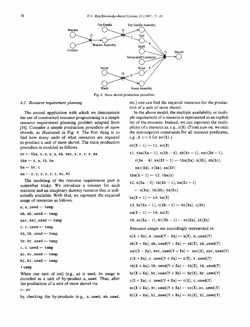
Top Handle Top Handle Assembly

Bracket t3 ~ t2

S c o o p - s h ~

Blade Scoop Assembly

Fig. 4. Snow shovel production procedure.

4.2. Resource requirement planning

The second application with which we demonstrate the use of constrained resource programming is a simple resource requirement planning problem adapted from [16]. Consider a simple production procedure of snow shovels, as illustrated in Fig. 4. The first thing is to find how many units of what resources are required to produce a unit of snow shovel. The main production procedure is modeled as follows.

sv ~- tha, n, n, n, n, sh, ssc, r, r, r, r, sa

tha +- n, n, th, ba

ba +- br, c

sa +- r, r, r, r, r, r, sc, bl

The modeling of the resource requirement part is somewhat tricky. We introduce a counter for each resource and an imaginary dummy resource that is unli- mitedly available. With that, we represent the required usage of resources as follows.

n, n_used +- temp

sh, sh_used +- temp

ssc, ssc_used +- temp

r, r_used +- temp

th, th_used +- temp

br, br_used +- temp

c, c_used +- temp

sc, sc_used +- temp

bl, bl_used +- temp

! t e m p

When one unit of nail (e.g., n) is used, its usage is recorded as a unit of by-product n_used. Thus, after the production of a unit of snow shovel via

o- s v

by checking the by-products (e.g., n_used, sh_used,

etc.) one can find the required resources for the production of a unit of snow shovel.

In the above model, the multiple availability or multiple requirement of a resource is represented as an explicit list of the resource. Instead, we can represent the multi- plicity of a resource as, e.g., r(6). (From now on, we omit the non-negative constraints for all resource predicates, e.g., X > = 0 for sv(X).)

sv(x + 1) t l , sv(x)

t l , tha(Xa -- 1), n(Xb - 4), sh(Xc -- 1), ssc(Xd - 1),

r(Xe -- 4), sa(Xf -- 1) ~-- tha(Xa), n(Xb), sh(Xc),

ssc(Xd), r(Xe), sa(Xf)

tha(x + 1) t2, the(x)

t2 , n ( X a - 2), th(Xb - 1), ba(Xc - 1)

+-- n(Xa), th(Xb), ba(Xc)

ba(X + 1) *-- t3, ba(X)

t3, br(Xa - 1), c(Xb - 1) ~- br(Xa), c(Xb)

sa(X + 1) +-- t4, sa(X)

t4, s c ( X a - 1), bZ(Xb- 1) +- sc(Xa), bl(Xb)

Resource usagcs arc accordingly represented as:

n(X + Xa), n_used(Y + Xa) ~-- n(X), n_used(Y)

sh(X + Xa), sh_used(Y + Xa) +- sh(X), sh_used(Y)

ssc(X + Xa), ssc_used(Y + Xa) +- ssc(X), ssc_used(Y)

r(X + Xa), r_used(Y + Xa) +- r(X), r_used(Y)

th(X + Xa), th_used(Y + Xa) +- th(X), th_used(Y)

br(X -5 Xa), br_used(Y -5 Xa) +- br(X), br_used(Y)

c(X -5 Xa), c_used(Y -5 Xa) ~-- c(X), c_used(Y)

sc(X -5 Xa), sc_used(Y -5 Xa) +- sc(X), sc_used(Y)

bl(X -5 Xa), bl_used(Y -5 Xa) +- BI(X), bl_used(Y)

Table 1 Time requirement for shovel production

Y.U. Ryu/Knowledge-Based Systems 10 (1997) 71 80

Resource Time Resource Time units units

shovel assembly 1 shaft 9 top handle assembly 1 scoop-shaft connector 5 top handle 7 rivet 4 bracket assembly 1 scoop assembly 1 bracket 1 scoop 2 coupler 9 blade 1 nail 1

For instance, assume there is a production division that assembles top handles. It has 25 units of top handle assemblies, 22 units of top handles, 4 units of nails, 27 units of bracket assemblies, 15 units of brackets, and 39 units of couplers in stock. Suppose it is required to deliver 100 units of top handle assemblies. Query

c- tha(lO0)

performs the task, resulting in net resource requirements of 53 units of top handles, 146 units of nails, 33 units of brackets, and 15 units of couplers.

Suppose preparations of resources require time units as specified by Table 1. We assume that there is no restriction on manpower and production facility so that each resource's production time is not affected by others unless there is a precedent relationship. We specify each resource as

resource_name(total_time_requirement,

unit_ time_ requirement)

where unit_time_requirement is time required to prepare the resource all preceding resources are ready and t o t a l _ t i m e _ r e q u i r e m e n t is the time required to prepare the resource and all preceding resources, counted from the beginning the whole production procedure. We modify the above production procedure model as follows:

sv(max(Tl, T2, T3, Td, T5, T6) + i, i)

~- tha(T1, _), n(T2, _), n(T2, _), n(T2, _),

n(T2. _), sh(T3, _), ssc(Td, _), r(T5, _),

r(T5, ), r (T5,_) , r (T5,_) , sa(T6,_)

tha(max(Tl, T2, T3) + i, I)

~-- n(T1, _), n(T1, ), th(T2, _), ba(T3, _)

ba(max(T1,T2) + l, 1) ~ br(T1, _), c(T2, _)

sa (max(T1 , T2, T3) + 1, 1)

~ - - r (T1 , _) , r (T1 , _ ) , r ( T 1 , _) , r (T1 , _) ,

r(T1, ), r(T1, _), sc(T2, _), bl(T3, _)

n(1, 1), n used ~-- tamp

sh(9, 9), sh_used ~- temp

sac(5, 5), sac_used ~- temp

r(4~4), r used+-temp

th(7~ 7), th_used +- temp

br(l~ I)~ br_used +- temp

c(9,9), c used~-temp

sc(2~ 2)~ so_used ~-- temp

bl(l~ I), bl_used ~- temp

!temp

Query

o- sv(T, _)

79

returns the total time unit required to produce a shovel; that is T = 12. The latest start time for the preparation of a resource is obtained by the following:

sv_time(T -- TU) +- ©sv(T, TU)

tha_time(Tl - TU) ~- ©tha(,TU), sv time(Tl)

ba_time(Tl -- TU) ~- ©ba(_, TU), tha_time(Tl)

sa_time(Tl - TU) ~- ©sa(_, TU), sv_time(Tl)

n_time(min(Tl, T2) - TU)

~-- ©n(_, TU), sv_time(T1), tha_t ime(T2)

sh_time(T1 - U) ~- @sh(_, TU), sv_time(Tl)

ssc_time(Tl - U) ~- ©sac(_, TU), sv_time(Tl)

r time(min(Tl, T2) - TU)

~-©r(_:TU)~ sv_time(Tl), sa time(T2)

th_time(Tl - U) ~- ©th(_,TU), tha time(T1)

br time(TI-U) ~-©br(_,TU),ba time(Tl)

c_time(Tl - U) +- @c(_, TU), ba time(Tl)

sc_time(Tl - U) ~- ©sc(_, TU), sa time(Tl)

bl_time(Tl - U) *- ©bl(_,TU), sa_time(Tl)

The earliest start time for the preparation of a resource is similarly obtained.

5. Concluding remarks

A knowledge representation method for constrained resources, inspired by linear logic, is presented and its computational model is proposed in the constraint logic programming scheme. We also present constrained resource programming as a specialized Petri net language, which is useful for the reachability test. Currently, constrained resource programming is

80 Y.U. Ryu/Knowledge-Based Systems 10 (1997) 71 80

partially implemented in a constraint logic programming language CLP(9~). It supports the Prolog-style interface and the backtracking mechanism.

The primary use of constrained resource programming is in the modeling of resource-oriented systems, such as production systems and resource allocation applications. We demonstrated its application to a multilateral trade matching problem and a resource requirement planning problem. As a more sophisticated application of constrained resource programming, a support system for job shop scheduling is under development. The goal of the support system is to help properly schedule job shops fulfilling demands (such as quantity and time) and minimizing costs in the existence of uncertainty, such as quantity/time demand change, machine break- down, operational tardiness, reworking, and machine bottleneck change. We view that job shop scheduling is not a one-time task. As the environment changes, at least part of the job shop can be reconfigured in order to adapt to the change; and the system advises reconfigura- tion of the job shop while the producing is on-going.

References

[1] J.L. Peterson, Petri nets, ACM Comput. Surv., 9 (1977) 223-252. [2] E.S. Buffa, Modern Production/Operations Management, John

Wiley, New York, NY, 7th edn, 1983. [3] J.M. Henderson and R.E. Quandt, Microeconomic Theory: A

Mathematical Approach, McGraw-Hill, New York, NY, 3rd edn, 1980.

[4] G. Hunter, Metalogic: An Introduction to the Metatheory of Standard First Order Logic, University of California Press, Berkeley, CA, 1971.

[5] R. Kowalski, Predicate logic as programming language, in J.L. Rosenfeld (ed.), Proc. IFIP 74, 1974, pp. 569-574.

[6] S.O. Kimbrough and R.M. Lee, Logic modeling as a tool for management science, Decision Support Systems, 4 (1988) 3 16.

[7] R. Bharath, Logic programming: A tool for MS/OR?, Interface, 16 (1986) 80-91.

[8] J. Jaffar and J.L. Lassez, Constraint logic programming, in Proc. Fourteenth ACM Symp. of the Principles of Programming Languages, Munich, Germany, 1987, pp. I 11-119.

[9] J.Y. Girard, Linear logic, Theoretical Computer Science, 50 (1987) 1-102.

[10] P.D. Lincoln, Linearlogic, ACM SIGACT, 23 (Spring 1992) 29-37. [11] J. Cohen, Constraint logic programming languages, Commun.

ACM, 33 (1990) 52-68. [12] A. Colmerauer, An introduction to Prolog III, Commun. ACM,

33 (1990) 69-90. [13] J.L. Peterson, Petri Net Theory and the Modeling of Systems,

Prentice-Hall, Englewood Cliffs, NJ, 1981. [14] L.S. Shapley and M. Shubik, The assignment game I: The core,

International Journal of Game Theory, 1 (1972) 111-130. [15] G.L. Thompson, Pareto optimal, multiple deterministic methods

for bid and offer auctions. Methods of Operations Research, 35 (1979) 517 530.

[16] T.E. Vollmann, W.L. Berry and D.C. Whybark, Manufacturing Planning and Control Systems, Irwin, Burr Ridge, IL, 3rd edn, 1992.

Young U. Ryu has been Assistant Professor of Infor- mation Systems at the Department of Decision Sciences, The University of Texas at Dallas since 1992. He received a Ph.D. degree in Management Science and Information Systems from The Uni- versity of Texas at Austin, where he had been Assist- ant Instructor for four years. He also has an MBA degree in Engineering Management and a BS degree in Mechanical Engineering. His research interests include logic-based modeling of normative systems, automation of legal decision making procedures, defeasible reasoning, artificial intelligence applications, and constraint logic modeling of systems.

logic-based representation and reasoning about knowledge of constrained resources

Documents