logic and logic programming - department of computer science · 2016-08-18 · logic programming...

Logic P r o g r a m m i n g

Logic and Logic Programming

J.A. Robinson

L ogic has been around for a very long time [23]. It was already an old subject 23 centuries ago, in Aristotle's day (384-322 BC). While Aristotle was not its origina-

tor, despite a widespread impres- sion to the contrary, he was cer- tainly its first important figure. He placed logic on sound systematic foundations, and it was a major course of study in his own university in Athens. His lecture notes on logic can still be read today. No doubt he taught logic to the future Alexander the Great when he served for a time as the young prince's personal tutor. In Alexan- dria a generation later (about 300 B.C.), Euclid played a similar role in systematizing and teaching the geometry and number theory of that era. Both Aristotle's logic and Euclid's geometry have endured and prospered. In some high schools and colleges, both are still taught in a form similar to their original one. The old logic, however, like the old geometry, has by now evolved into a much more general and powerful form.

Modern ('symbolic' or 'mathematical') logic dates back to 1879, when Frege published the first version of what today is known as the predicate calculus [14]. This system provides a rich and comprehensive notation, which Frege intended to be adequate for the expression of

all mathematical concepts and for the formulation of exact deductive reasoning about them. It seems to be so. The principal feature of the predicate calculus is that it offers a precise characterization of the con- cept of proof. Its proofs, as well as its sentences and its other formal expressions, are mathematically de- fined objects which are intended not only to express ideas meaning- ful ly--that is, to be used as one uses a language--but also to be the subject matter of mathematical analysis. They are also capable of being manipulated as the data objects of construction and recognition algorithms.

At the end of the nineteenth cen- tury, mathematics had reached a stage in which it was more than ready to exploit Frege's powerful new instrument. Mathematicians were opening up new areas of research that demanded much deeper logical understanding and far more careful handling of proofs, than had previously been required. Some of these were David Hiibert's abstract axiomatic recast- ing of geometry and Giuseppe Peano's of arithmetic, as well as Georg Cantor's intuitive explorations of general set theory, espe- cially his elaboration of the dazzling theory o f transfinite ordinal and cardinal numbers. Others were Ernst Zermelo's axiomatic analysis of set theory following the discov-

ery of the logical and set-theoretic paradoxes (such as Bertrand Rus- sell's set of all sets which are not members of themselves, which therefore by definition both is, and also is not, a member of itself); and the huge reductionist work Prin- cipia Mathematica by Bertrand Rus- sell and Alfred North Whitehead. All of these developments had either shown what could be done, or had revealed what needed to be done, with the help of this new logic. But it was necessary first for mathematicians to master its techniques and to explore its scope and its limits.

Significant early steps toward this end were taken by Leopold Lowenheim (1915), [29] and Thoralf Skolem [45], who studied the symbolic "satisfiability" of formal expressions. They showed that sets of abstract logical conditions could be proved consistent by being given specific interpretations con- structed from the very symbolic expressions in which they are formulated. Their work opened the way for Kurt G6del (1930, [17]) and Jacques Herbrand (1930, [19]) to prove, in their doctoral disserta- tions, the first versions of what is now called the completeness of the predicate calculus. G6del and Herbrand both demonstrated that the proof machinery of the predicate calculus can provide a formal proof for every logically true prop-

COMMUNICATIONS OF THE ACM/March 1992/Vol.35, No.3 41

Logic P r o g r a m m i n g

osition, and indeed they each gave a constructive method for f inding the proof, given the proposition. G6del's more famous achievement, his discovery in 1931 of the amazing ' incompleteness theorems' about formalizations of arithmetic, has tended to overshadow this impor tant earl ier work of his, which is a result about pure logic, whereas his incompleteness results are about certain appl ied logics (formal axiomatic theories of e lementary number theory, and similar systems) and do not directly concern us here.

The completeness of the predicate calculus links the syntactic p roper ty of formal provability with the conceptually quite di f ferent semantic p roper ty of logical truth. I t assures us that each proper ty be- longs to exactly the same sentences. Formal syntax and formal semantics are both needed, but for a time the spotlight was on formal syntax, and formal semantics had to wait until Alfred Tarski (1934, [46]) in- t roduced the first r igorous semanti- cal theory for the predicate calculus, by precisely def ining satisfiability, truth (in a given interpretation), logical consequence, and o ther related notions. Once it was filled out by the concepts of Tarski's semantics, the theory of the predicate calculus was no longer unbalanced. Shortly af terward Ger- hard Gentzen (1936, [15]) fur ther sharpened the syntactical results on provability by showing that if a sentence can be proved at all, then it can be proved in a 'direct ' way, without the need to introduce any extraneous 'clever' concepts; those occurr ing already in the sentence itself are always sufficient.

All of these positive discoveries of the 1920s and 1930s laid the foundat ions on which today's predicate calculus theorem-proving programs, and thus logic programming have been built.

Not all the great logical discoveries of this per iod were positive. In 1936 Alonzo Church and Alan Tur ing (see [6, 47]) independent ly discovered a fundamenta l negative

proper ty of the predicate calculus. There had until then been an in- tense search for a positive solution to what Hilbert called the decision problem--the problem to devise an algori thm for the predicate calculus which would correctly determine, for any formal sentence B and any set A of formal sentences, whether or not B is a logical consequence of A. Church and Tur ing found that despite the existence of the p roof procedure , which correctly recog- nizes (by constructing a p roof of B from A) all cases where B is in fact a logical consequence of A, there is not and cannot be an algori thm which can similarly correctly recog- nize all cases in which B is not a logical consequence of A. The i r discovery bears directly on all at tempts to write theorem-proving software. It means that it is pointless to try to p rogram a computer to answer 'yes' or 'no' correctly to every question of the form 'is this a logically true sentence?' The most that can be done is to identify useful subclasses of sentences for which a decision procedure can be found. Many such subclasses are known. They are called 'solvable subcases of the decision problem' , but as far as I know none of them have tu rned out to be of much practical interest.

When World War II began in 1939 all the basic theoretical foundations of today's computat ional logic were in place. What was still lacking was any practical way of actually carrying out the vast symbolic computat ions called for by the p roof procedure. Only the very simplest of examples could be done by hand. Already there were those, h o w e v e r - - T u r i n g himself for o n e - - who were making plans which would eventually fill this gap. Tur- ing's method in negatively solving the decision problem had been to design a highly theoretical, abstract version of the modern stored- program, genera l -purpose universal digital computer (the 'universal Tur ing machine'), and then to prove that no p rogram for it could realize the decision procedure . His subsequent leading role in the war-

t ime British code-breaking project included his part icipation in the actual design, construction and operat ion of several electronic machines of this kind, and thus he must surely be reckoned as one of the major pioneers in their early development .

Logic on the Computer Apar t from this enormously important cryptographic intelligence work and its crucial role in ballistic computat ions and nuclear physics simulations, the war-time development of electronic digital computing technology had relatively little impact on the outcome of the war itself. After the war, however, its rap id commercial and scientific exploitat ion quickly launched the current computer era. By 1950, much- improved versions of some of the war-time genera l -purpose electronic digital computers became available to industry, univer- sities and research centers. By the mid-1950s it had become apparen t to many logicians that, at last, sufficient comput ing power was now at hand to suppor t computat ional exper iments with the predicate calculus p roo f procedure . I t was jus t a mat ter of p rog ramming it and trying it on some real examples. Sev- eral papers describing projects for doing this were given at a Summer School in Logic held at Cornell University in 1957. One of these [37, pp. 74-76] was by Abraham Robinson, the logician who later surpr ised the mathematical estab- l ishment by applying logical 'non- s tandard ' model theory to legiti- mize infinitesimals in the foundat ions of the integral and dif- ferential calculus. Other published accounts of results in the first wave of such exper iments were [12, 16, 35, 49]. The re had also been, in 1956, a s trange exper iment by [33] which at tracted a lot of attention at the time. It has since been cited as a milestone of the early stages o f artificial intelligence research. The authors designed their 'Logic The- ory Machine' p rogram to prove sentences of the proposi t ional cal-

4 2 March 1992/Voh35, N o . 3 / C O M M U N I C A T I O N S OF TH e= ACM

culus (not the full predicate calculus), a very simple system of logic for which there had long existed well-known decision procedures. They nevertheless explicitly re- jected the idea of using any algorithmic proof procedure, aiming, instead, at making their program behave 'heuristically' as it cast about for a proof. This experiment was intended to model human problem-solving behavior, taking propositional calculus theorem- proving in particular as the problem-solving task, rather than to program the computer to prove propositional calculus theorems efficiently.

No sooner were the first computational proof experiments carried out than the severe combinatorial complexity of the full predicate calculus proof procedure come vividly into view. The procedure is, after all, essentially no more than a systematic exhaustive search through an exponentially expanding space of possible proofs. The early researchers were brought face-to-face with the inexorable 'combinatorial explosion' caused by conducting the search on nontrivial examples. These first predicate calculus proof-seeking programs may have inspired, and perhaps even de- served, the disparaging label 'Brit- ish Museum method' (see [33]), which was destined to be pinned on any merely-generate-and-test procedure which blindly and undis- criminatingly tries all possible com- binations in the hope that a winning one, or even an acceptable one, may eventually turn up.

The intrinsic exponential complexity of the predicate calculus proof procedure is to be expected, because of the nature of the search space. There is evidently little one can do to avoid its consequences. The only reasonable course is to look for ways to strengthen the proof procedure as much as possible, by simplifying the forms of expressions in the predicate calculus and by packing more power into its inference rules. This might at least make the search process more

efficient, and permit it to find proofs of more interesting examples before it runs into the exponential barrier.

Some limited progress has been made in this direction by reorganizing the predicate calculus in various 'machine-oriented' versions.

Evolution of Machine- Oriented Logic The earliest versions of the predicate calculus proof procedure were all based on human-oriented reasoning pa t te rns- -on types of inference which reflected formally the kind of 'small' reasoning steps which humans find comfortable. A well- known example of this is the modus ponens inference-scheme. In using modus ponens, one infers a conclusion B from two premisses of the form A and (if A then B). Such human-oriented inference-schemes are adapted to the limitations--and also to the s t rengths- -of the human information-processing system. They therefore tend to involve simple, local, small and perceptually immediate features of the state of the reasoning. In particular, they do not demand the handling of more than one such bundle of features at a t ime-- they are designed for serial processing on a single processor. The massive parallelism in human brain processes is well below the level of conscious awareness, and it is of the essence of deductive reasoning that the human reasoner be fully conscious of the 'epistemologi- cal flow' of the proof and of its stepwise assembling of his or her assent and understanding. In logics based on such fine-grained serial inference patterns, proofs of interesting propositions will tend to be large assemblies of small steps. The search space for the corresponding proof procedures will accordingly tend to be dense and overcrowded with redundant alternatives at too low a level of detail.

By about 1960 it had become clear that it might be necessary to abandon this natural predilection for human-oriented inference patterns, and to look for new logics

based on larger-scale, more complex, less local, and perhaps even highly parallel, machine-oriented types of reasoning. In contemplat- ing these possible new logics it was hoped their proofs would be shorter and (at the top level) simpler than those in the human- oriented logics. Of course, in the interior of any individual inference, there would presumably be a large amount of hidden structural detail. The global search space would be sparser, since it would need to contain only the top-level structure of proofs. The proof procedure itself would not need to be concerned with the copious details of the conceptual microstructure packaged within the inference steps.

This was the motivation behind the introduction, in the early 1960s, of a new logic, based on two highly machine-oriented reasoning patterns: unification, and the various kinds of resolution which incorpo- rate it.

clausal Logic The 1960 paper [12] had already drawn attention to the simplified clausal predicate calculus in which every sentence is a clause. (A clause is a sentence with a very simple form: it is just a--possibly emp ty - - disjunction of literals. A literal, in turn, is just the application of an unnegated or negated predicate to a suitable list of terms as arguments). In the same year, Dag Prawitz [34] had also forcefully advocated the use of the process which we now call unification. Along with Stig Kanger (see [34, footnote 11], p. 170) he apparently had independently rediscovered unification in the late 1950s. He apparently did not realize that it had already been introduced by Herbrand in his thesis of 1930 (al- beit only in a brief and rather ob- scure passage). These were major steps in the right direction. Neither the Davis-Putnam nor the Prawitz improved proof procedures, however, went quite far enough in dis- carding human-oriented inference patterns, and their algorithms still

COMMUNI~LTIONS OF THE ACM/March 1992/Vol.35, No.3 4 3

Log ic P r o g r o m m i n g became bogged down too early in their searches, to be useful.

This was the situation when I first became interested in mechanical theorem-proving in late 1960. From 1961 to 1964 I worked each summer as a visiting researcher at the Argonne National Laboratory 's Appl ied Mathematics Division, which was then directed by William F. Miller. It was Bill Miller who in early 1961 first in t roduced me to the engineer ing side of predicate calculus theorem-proving by point- ing out to me the Davis and Putnam paper. He invited me to spend the summer of 1961 at Argonne as a visiting researcher in his division, with the suggested assignment of p rogramming the Davis-Putnam proof procedure on the IBM 704 and more generally of pursuing mechanical theorem-proving research.

Reading the Davis-Putnam paper [12] in early 1961 really changed my life. Al though Hilary Putnam had been one of my advisers when I was working on my doctoral thesis in philosophy at Princeton (1953- 1956), my research had dealt with David Hume's theory of causation and had little or nothing to do with modern logic, to which I paid scant attention at that time. I did not find out about Putnam's interest in the predicate calculus p roof procedure until I read this paper , four years after I had left Princeton. It is a very impor tant paper . They showed how, by relatively simple but ingenious algorithmic reorgani- zation, the original naive predicate calculus p roof procedure of He rb rand could be vastly improved.

In a 1963 paper I wrote about my 'combinatorial explosion' experience with p rogramming and run- ning the Davis-Putnam procedure in For t ran for the IBM 704 at Ar- gonne [38, pp. 372-383]. Mean- while, dur ing my second research summer there (1962) an Argonne physicist who was interested in and very knowledgable about logic, Wil- liam Davidon, had drawn my attention to the impor tant 1960 paper by Dag Prawitz [34], in which I first

encountered the idea of unification. After struggling with the woe- ful combinatorial inefficiency of the instantiation-based procedure used by Davis and Putnam (and by everybody else at that time; it goes back to Herbrand ' s so-called 'Prop- erty B Method' developed in [19]). I was immediately very impressed by the significance of this idea. It is essentially the idea under lying Herbrand ' s 'Proper ty A Method ' developed in the same thesis. Here again was still another paper showing that even vaster improvements than those flowing from the Davis and Putnam paper were possible over the 'naive' predicate calculus p roof procedure . Instead of generat ing-and-test ing successive instan- tiations (substitutions) hoping eventually to hit upon the r i g h t ones, Prawitz was describing a way of directly computing them. This was a breakthrough. It offered an elegant and powerful alternative to the blind, hopeless, enumerat ive 'Brit- ish Museum' methodology, and pointed the way to a new methodology featur ing deliberate, goal- directed constructions.

The entire academic year of 1962-1963 was consumed in trying to figure out the best way to exploit this Herbrand-Kanger-Prawi tz process effectively, so as to eliminate the generat ion of irrelevant instances in the p roof search. Finally, in the early summer of 1963, I managed to devise a clausal logic with a single inference scheme, which was a combination of the Herbrand-Kanger-Prawi tz process (for which I proposed the name unification) with Gentzen's 'cut' rule. This combination produced a ra ther inhuman but very effective new inference pattern, for which I p roposed the name resolution. Reso- lution permits the taking of arbi- trarily large inference steps which in general require very consider- able computat ional effort to carry out (and in some cases even to unders tand and to verify). Most of the effort is concentrated on the unification involved. Preliminary investigations indicated that resolution-

based theorem-provers would be significantly bet ter than any which had been built previously.

I wrote about these ideas at Ar- gonne at the end of the summer of 1963, and sent the paper to the

Journal of the A.C.M. (JACM). It then apparent ly remained unread on some referee 's desk for more than a year. It required some urg- ing by the then edi tor of the Jour- nal, Richard H a mming o f Bell Lab- oratories, before the referee finally responded. The outcome was that the paper , [39], was published only in January 1965. Meanwhile the manuscr ipt had been circulating. In 1964 at Argonne , Larry Wos, George Robinson and Dan Carson p rog ra mme d a resolution-based theorem prover for the clausal predicate calculus, adding to the basic process search strategies (called unit preference and set of support) of their own devising, which fur ther speeded the resolution p roof process. Because of the refer- eeing delay, their paper , reached pr int before mine [52]) and could only cite it as 'to be published' .

T h r o u g h o u t the winter of 1963- 64, while waiting for news of the paper 's acceptance or rejection by JACM, I concentrated on trying to push the ideas further , and looked for ways of ex tending the resolution principle to accommodate even larger inference steps than those sanctioned by the original binary resolution pattern. One of these tu rned out to be particularly attrac- tive. I gave it the name hyper-resolution, meaning to suggest that it was an inference principle on a level above resolution. One hyperresolution was essentially a new integrated whole, a condensat ion of a deduction consisting of several reso- lutions. The paper describing hyperresolut ion was published at about the same time as the main resolution paper , and was later re- pr in ted in [40, pp. 416-423].

It had been my guiding idea in this research that bigger and (computationally) better inference patterns might be obtained by some- how packaging entire deductions at

4 4 March 1992/Vo1.35, No,3/COMMUNICATIONS OF THE A C M

one level into single inferences at the next higher level. As I cast about for such patterns I came across a quite restricted form of r eso lu t ion- - I called it 'P l - reso lu t ion ' - -which I found I could prove was just as powerful as the original unrestricted binary resolution. The restriction in Pl-resolut ion is that one of the two premises must be an unconditional clause, that is, a clause in which there are no negative literals (or what amounts to the same thing, a sentence of the form: ' if antecedent then consequent' whose antecedent part is empty). From this restriction, it follows that every P l -deduction (that is, a deduct ion in which every inference is a Pl-resolut ion) can always be decomposed into a combination of what I called 'P2- deductions' . A P2-deduction is a P 1-deduction which satisfies the extra restriction that its conclusion, and all of its premises except one, are uncondit ional clauses. Thus, exactly one conditional clause is involved as an 'external ' clause in a P2-deduction. By ignoring the in- ternal inferences of a P2-deduction tree and deeming its conclusion to have been directly obtained from its premises, we obtain a single large i n f e r ence - - a hyper reso lu t ion - - which is really a multi inference deduct ion whose interior details are hidden from view inside a sort of logical black box.

Computational Logic: The Resolution Boom After the publication of the paper in 1965, there began a sustained drive to program resolution-based proof procedures as efficiently as possible and to see what they could do. In Edinburgh, Bernard Melt- zer's Computational Logic group and Donald Michie's Machine Intelligence group had by 1967 attracted many young researchers who have since become well known and who at that time worked on various theoretical and practical resolution issues: Robert Kowalski, Patrick Hayes, the late Donald Kuehner , Gordon Plot- kin, Robert Boyer and J Moore, David H.D. Warren, Maarten van

Emden, Robert Hill. Bernard Meit- zer had visited Rice University for two months in early 1965 in o rde r to study resolution intensively, and on his re turn to Edinburgh he set up one of two seminal research groups which were to foster the birth of logic p rogramming (the other being Alain Colmerauer 's group in Marseille). Thus began my long and fruitful association with Edinburgh. By 1970 the resolution boom was in full swing. I recall that in that year Keith Clark and Jack Minker were among those attend- ing a N A T O Summer School organized by Bernard Meltzer and Nic- olas Findler at Menaggio on Lake Como. The re we preached the new 'resolution movement ' for two weeks, and Clark and Minker de- cided to jo in it, soon becoming two notable contributors.

Meanwhile, however, in the U.S., the reaction was mostly muted, except for isolated pockets of enthusi- asm at Argonne, Stanford, Rice and a few other places. Bill Miller had left Argonne to go to Stanford at the end of 1964, and I accepted his invitation to spend the summers of 1965 and 1966 as a visiting researcher in his computat ion group at the Stanford Linear Accelerator Center. It was at Stanford in the summer of 1965 that I met John McCarthy for the first time. I was astonished to learn that after he had recently read the resolution paper he had written and tested a complete resolution theorem- proving p rogram in Lisp in a few hours. I was still p rogramming in Fortran, and I was used to taking days and even weeks for such a task. In 1965, however, one could use Lisp easily in only a very few places, and nei ther Rice University nor Argonne National Laboratory were then among them.

Ber t ram Raphael, Nils Nilsson, and Cordell Green, at Stanford Research Institute, were building deductive databases for the 'STRIPS' p lanning software for their robot, and they were adopt ing resolution for this (see [36]). At New York University, Martin Davis

and Donald Loveland were developing Davis's very closely related unification-based ' l inked conjunct ' method [10, pp. 315-330] in ways which eventually led Loveland independent ly to his Model Elimina- tion system [28], a linear reasoning method entirely similar to the linear resolution systems developed by the Edinburgh group, and by David Luckham at Stanford [30]. Back at Argonne, Larry Wos and George Robinson had formed a very strong 'automated deduct ion ' group. They broadened the applicability of unification by augment ing resolution with fur ther inference rules specialized for equality reasoning (mod- ulation, paramodulation) which further improved the efficiency of p roof searches [43]. Today, the Argonne group is still f lourishing and remains a major center of ex- cellence in automated deduction.

In 1969 there began a series of noisy but interesting (and, it later turned out, fruitful) academic skir- mishes between the then somewhat meagerly funded resolution community and MIT's Artificial Intelli- gence Laboratory led by Marvin Minsky and Seymour Papert. The MIT AI Laboratory at that time was (it seemed to us) comfortably, if not lavishly, suppor ted by the Penta- gon's Advanced Research Projects Agency (then ARPA, now DARPA). The issue was whether it was better to represent knowledge computationally, for AI purposes, in a declarative or in a procedural form. I f it was the former (as had been origi- nally proposed in 1959 by John McCarthy) [31] then it would be the predicate calculus, and efficient p roof procedures for it, that would play a central role in AI research. I f it was the latter (e.g., see [51]), then a computat ional realization of knowledge would have to be a system of procedures 'heterarchically' organized so that each could be in- voked by any of the others, and indeed by itself. These procedures would be 'agents ' that would both cooperate and compete in collec- tively accomplishing the various tasks compris ing intelligent behav-

C O M M U N I C A T I O N S O F T H E ACM/March 1992/Vol.35, No.3 45

LOgic P r o g r o m m i n g ior and thought.

Minsky's book, The Society of the Mind [32], elegantly summed up the MIT side of this debate in es- chewing polemics to outline a grand unified theory of the structure and function of the mind in the tradition of Freud and Piaget. The logic side of the debate has been definitively treated in [25], which eloquently sets forth the role of logic in the computational orga- nization of knowledge and banishes the procedural-declarative dichot- omy by insight that Horn clauses (that is, clauses containing at most one unnegated literal) can be inter- preted as procedures, and thus can be activated and executed by a suitably designed processor. It is this insight that underlies what we now call logic programming.

The never-to-be-implemented but influential 'Planner' system by Carl Hewitt--his first paper on Planner, in [20]--epitomized the MIT procedural approach, while the QA ('Question-Answering') series of programs by [31] carried out McCarthy's logical 'Advice Taker' approach to AI and convinced many skeptics that it would really work. The work by [18] should now be seen and appreciated as the earliest demonstration of a logic programming system. That paper illus- trated how to adapt a resolution-based proof procedure to provide an assertion-and-query facility in all essential respects like that provided by the later Prolog systems. Unfortunately, the system was built on the rapidly ramifying full resolution scheme, using unrestricted (rather than Horn-) clauses, so that the program suffered from premature combinatorial explo- siveness. Nevertheless, it was largely Green's pioneering work of [18] that encouraged Kowalski and the Edinburgh group to fight off the MIT 'procedural-is-best' attack by developing the highly efficient (LUSH, later called SLD), slowly ramifying linear resolution systems for the restricted case o f Horn- clauses [27, pp. 542-577].

The procedural-logical fight was really ended, in a delightfully unex- pected way, by Kowalski's inspired procedural interpretation of the behavior of a Horn-clause linear resolution proof finder, [24]. He pointed out that in view of the behavior of Horn clause linear-resolution proof-seeking processes, a collection of Horn clauses could be regarded as knowledge organized both declaratively and procedurally. It suddenly was hard to see what all the fuss had been about. Kowalski was led to this reconciliatory principle by superb implementation of a 'structure-sharing' resolution theorem prover at Edinburgh [5, pp. 101-116], which suddenly completed the transformation .of theorem-proving from generate-and-test searching to goal-directed stack-based computation. When restricted to Horn clauses, the Boyer-Moore approach becomes the obvious pre- cursor of the first implementations of Prolog. David H.D. Warren's enormously influential later software and hardware refinements and advances clearly descend directly from the Boyer-Moore methodology [50].

Only the interaction of the Edin- burgh group's ideas with the work of Colmerauer's Montreal [7] and Marseilles [8] groups was required to open up logic programming and launch it on its meteoric career. The interesting story o f this interaction was published by [26]. Logic programming is today in excellent health. The logic programming community has settled down to enjoy, after two decades of very rapid growth, a steady mature round of professional conferences and workshops, a plentiful flow of research and expository publication in books and in its own and other journals, an exciting marketplace of new software and hardware enter- prises, and such majestic long- range national and international undertakings as Japan's Fifth Gen- eration Project and those spon- sored by the European Commu- nity.

A Closer Look at Unification and Resolution What then, is the resolution-based clausal predicate calculus, and what is unification and how does it work?

Clauses Davis's and Putnam's clauses are quite expressive, despite their apparently restricted form. This is reflected in the many different but equivalent ways in which one can write them. In dealing with clauses computationally, however, it is best to keep them simple and to work with them abstractly.

A clause can in general be taken to be a sentence o f the form 'if P then Q', which we will usually write as P ~ Q or sometimes the other way round, as Q ~ P. The antecedent P is a set of conditions and the consequent Q is a set of conclusions. These conditions and the conclusions are atomic sentences. The order in which the atomic sentences per- force are presented in written versions of clauses and has no logical significance. There is usually no visible indication of the fact that the antecedent P is a conjunction of its conditions, while the consequent Q is a disjunction of its conclusions. Those two facts are assumed to hold by convention. In discussing inferences and manipulations involving clauses, the abstract view of P and Q as sets is both natural and convenient.

We can then classify a clause along three different dimensions, depending on whether its atomic sentences contain any variables or not, whether or not it has any conditions, and whether or not it has any conclusions. A clause with no variables is said to be a ground clause, while if it has one or more variables, it is called a general clause. A general clause is understood to be a universally quantified sentence, each of its variables being tacitly universally quantified with the whole sentence as scope. A clause with one or more conclusions is said to be a positive clause; while one with no conclusions is said to be a

46 March 1992/%1.35, No.3/COMMUNICATIONS O F T H E A C M

negative clause. Finally, a clause with one o r m o r e condi t ions is said to be a conditional clause; while one with no condi t ions is said to be an unconditional clause. ( T h e r e is only one clause that is both uncondi t iona l and negat ive: it is known as the empty clause.)

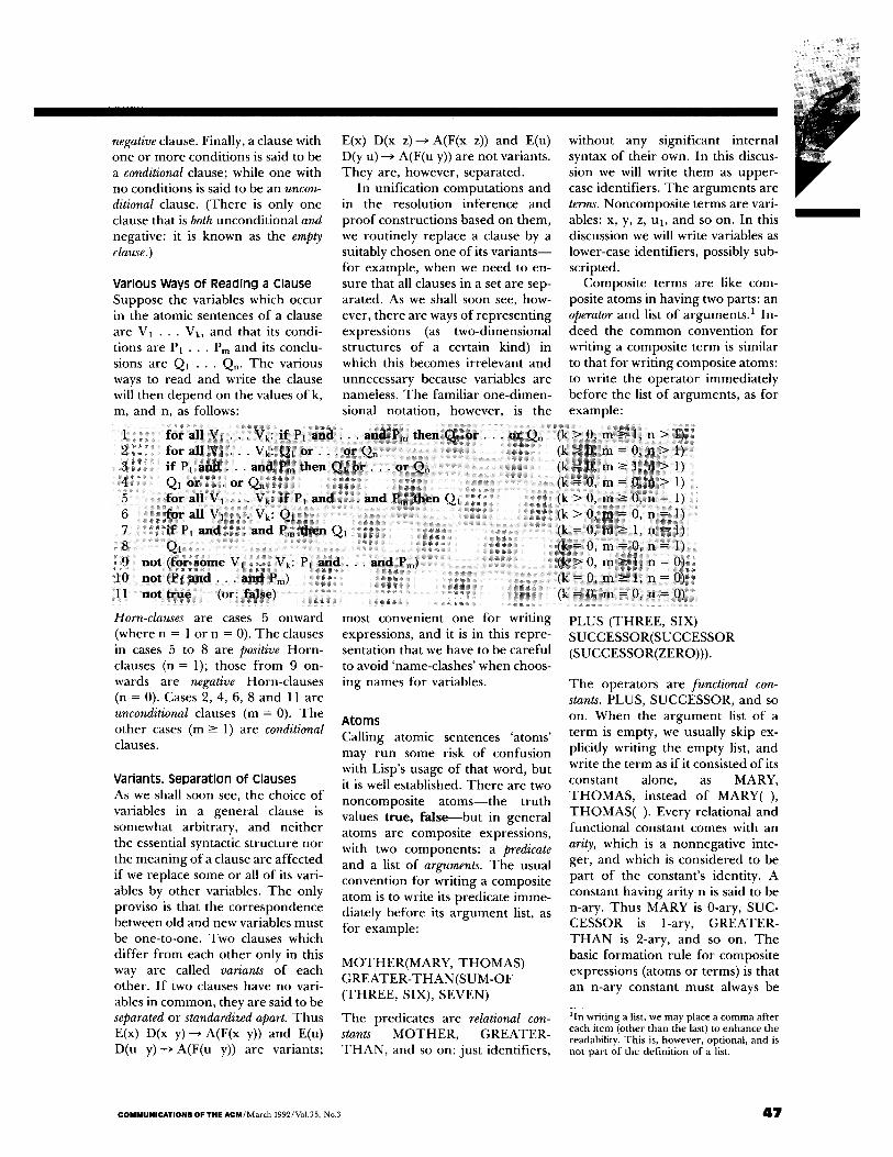
Various Ways of Reading a Clause Suppose the variables which occur in the atomic sentences o f a clause are V[ . . . Vk, and that its conditions are Pl • • - Pm and its conclusions are Ql . . . Qn. T h e var ious ways to read and write the clause will then d e p e n d on the values o f k, m, and n, as follows:

E(x) D(x z ) ~ A(F(x z)) and E(u) D(y u) ---> A(F(u y)) a re no t variants. T h e y are, however , separated.

In unif icat ion computa t ions and in the resolut ion in fe rence and p r o o f const ruct ions based on them, we rout ine ly replace a clause by a suitably chosen one o f its v a r i a n t s - - for example , when we need to en- sure that all clauses in a set a re separated. As we shall soon see, however, the re are ways o f r ep re sen t ing express ions (as two-dimens ional s t ructures o f a cer ta in kind) in which this becomes i r re levant and unnecessary because variables are nameless. T h e famil iar one -d imen- sional notat ion, however , is the

wi thout any significant in ternal syntax o f the i r own. In this discussion we will write t hem as uppe r - case identif iers . T h e a r g u m e n t s are terms. Noncompos i t e te rms are variables: x, y, z, ul , and so on. In this discussion we will write variables as lower-case identif iers , possibly sub- scripted.

Compos i te te rms are like com- posite a toms in having two parts: an operator and list o f a r g u m e n t s ) In- deed the c o m m o n conven t ion for wri t ing a composi te t e r m is similar to that for wri t ing composi te atoms: to write the o p e r a t o r immedia te ly be fo re the list o f a rguments , as for example :

1 for a l l V 1 . . . V k : i f P ~ a n d . . . a n d P m t h e n Q l o r . . o r Qn ( k > O , m ~ l , n > ~) 2 for all Vl . . . Vk: Q1 o r . . . o r Qn ik ~ O, m = O, n > l i 3 i f Pl a n d . . , a n d Pm t h e n Ql o r ~ . . o r Qn (k ~ O, m -> 1, n > 1)

7 i f PI a n d . , . a n d Pm t h e n Qt

10 no t (P~ a n d . . , a n d Pro) 11 n o t true (or: fa l se )

Horn-clauses are cases 5 onward (where n = 1 or n = 0). T h e clauses in cases 5 to 8 are positive Horn - clauses (n = 1); those f rom 9 on- wards are negative Horn-c lauses (n = 0). Cases 2, 4, 6, 8 and 11 are unconditional clauses (m = 0). T h e o the r cases (m > 1) are conditional clauses.

Variants. Separation of Clauses As we shall soon see, the choice o f variables in a genera l clause is somewhat arbi t rary, and ne i the r the essential syntactic s t ruc ture no r the m e a n i n g o f a clause are af fec ted if we replace some or all o f its variables by o the r variables. T h e only proviso is that the c o r r e s p o n d e n c e be tween old and new variables must be one- to-one . Two clauses which d i f fe r f rom each o the r only in this way are called variants of each other . I f two clauses have no variables in c o m m o n , they are said to be separated or standardized apart. T h u s E(x) D(x y ) ~ A(F(x y)) and E(u) D(u y)--> A(F(u y)) are variants;

most conven ien t one for wri t ing expressions, and it is in this repre - sentat ion that we have to be careful to avoid 'name-clashes ' when choos- ing names for variables.

A t o m s Call ing a tomic sentences 'a toms' may r u n some risk o f confus ion with Lisp's usage o f that word, but it is well established. T h e r e are two noncompos i t e a t o m s - - t h e t ru th values t rue , f a l s e - - b u t in genera l a toms are composi te expressions, with two componen t s : a predicate and a list o f arguments. T h e usual conven t ion for wri t ing a composi te a tom is to write its predica te immediately before its a r g u m e n t list, as for example :

M O T H E R ( M A R Y , T H O M A S ) G R E A T E R - T H A N ( S U M - O F ( T H R E E , SIX), SEVEN)

T h e predicates are relational constants M O T H E R , G R E A T E R - T H A N , and so on: jus t identif iers ,

PLUS ( T H R E E , SIX) S U C C E S S O R ( S U C C E S S O R (SUCCESSOR(ZERO))) .

T h e opera to r s are functional constants. PLUS, S U C C E S S O R , and so on. W h e n the a r g u m e n t list o f a t e r m is empty , we usually skip explicitly wri t ing the emp ty list, and write the t e rm as if it consis ted o f its constant alone, as MARY, T H O M A S , instead o f M A R Y ( ) , T H O M A S ( ) . Every relat ional and funct ional constant comes with an arity, which is a nonnega t ive integer, and which is cons idered to be par t o f the constant 's identity. A constant having arity n is said to be n-ary. T h u s M A R Y is 0-ary, SUC- C E S S O R is 1-ary, G R E A T E R - T H A N is 2-ary, and so on. T h e basic fo rma t ion rule for composi te express ions (atoms or terms) is that an n-ary constant must always be

q n wri t ing a list, we may place a c o m m a af ter each i t em (other t han the last) to e n h a n c e the readabili ty. Th is is, however , optional , and is not pa r t o f the defini t ion o f a list.

C O M M U N I C A T I O N S O F T H E ACM/March I992/Vol.35, No.3 4 7

LOgiC P r o g r a m m i n g followed immedia te ly by a list o f n a r gumen t s (except, as no ted above, when n = 0, when the list can be by conven t ion omitted). T h e c o m m o n u n d e r l y i n g semantic idea is that of an applicative expression which represents the result o f applying a func- t ion or relat ion to a suitable tuple of a rguments .

In the clausal predicate calculus, clauses are the only k ind of sentence available in which to express the premises and des i red conclusion of a p roo f problem. This is no t as l imit ing as it sounds. I t is in fact possible to t ranslate (automatically) a p roo f p rob lem from the full predicate calculus into the clausal predicate calculus. Detailed discus- sions of how to do this can be found , in [ 12].

Substitution Making the clausal predicate calculus more mach ine -o r i en ted calls for a m u c h closer analysis of the idea of instantiation. W h e n an expression B can be ob ta ined f rom ano the r expression A by subst i tu t ing terms for some or all o f the variables in A, B is said to be an instance of A.

For example , F( H(y z) G( H(y z ) A(y)) A(y)) is an instance of F(x G(x y) y). Inspec t ion conf i rms that F( H(y z) G(H(y z ) A(y)) A(y)) can be ob ta ined f rom F(x G(x y) y) by si- multaneously replac ing each occurrence of x and y by an occurrence of H(y z) and an occurrence of A(y) respectively. It is very in teres t ing that this basic logical opera t ion of substitution is essentially a parallel one.

We can represen t specific substi- tut ions by sets o f equat ions. For example , the p reced ing substi tu- t ion can be represen ted by the set {x = H(y z), y = A(y) }. Unspecif ied subst i tut ions are usually deno ted by lower-case Greek letters: 0, A, g, ~, and the result of apply ing a substi- tu t ion to an expression E is indicated by wri t ing E0, EA. There fo re , if E is F(x G)(x y) y) and 0 is {x = H(y z), y = A(y)}, E0 is F( H(y z) G( H(y z ) A(y)) A(y)).

Unification Let S be a set o f expressions. W h e n a subst i tu t ion 0 t ransforms every expression in S into the same expression, 0 is said to unify S (or to be a unifier of S) and the set S is said to be unifiable.

For example , let 0 be {x -- H(P Q), y = D, u = P, v = Q, z = G(H(P Q),D)}. W h e n we apply 0 to the two expressions F(x G(x y)) and F(H(u v) z) both of them become the same expression, namely F( H(P Q) G(H(P Q) D)). T h u s 0 unifies the set {F(x G(x y)), F(H(u v) z)}.

This set, however, is also un i f ied by the subst i tu t ion tr = {x = H(u v), z = G( H(u v) y)}, which t rans forms both its mem ber s into the same expression: F(H(u v) G(H(u v) y)). This express ion is no t only a more genera l c o m m o n instance of F(x G(x y)) a n d F(H(u v) z), bu t is actually a most genera l c o m m o n instance, a n d so cr represents the most genera l way in which the set {F(x G(x y)), F(H(u v) z)} can be unif ied. We therefore say it is a most general unifier ( 'mgu') o f {F(x G(x y)), F(H(u v) z)}. All o ther c o m m o n instances of F(x G(x y)) and F(H(u v) z) are instances of the above most genera l one. In this par t icular case we have: F(H(u v) z)0 = F(x G(x y))0 = F(H(P Q) G(H(P Q) D)) = (F(x G(x y))cr)g = F(H(u v) G(H(u v) y)/x where /x = {u = P, v = Q, y = D}. This suggests that 0 is some kind of ' p roduc t ' o f the m g u ~ and the subst i tu t ion g. We can write 0 explicitly as 0 = cr./~ an d we f ind that, indeed , this no- t ion of the p roduc t o f two substi tu- tions can be na tura l ly de f ined and is ext remely useful.

T h e product a'/3 of two substi tu- tions a and /3 is the overall substi tu- t ion which results f rom first per- fo rming a and then pe r fo rming /3 . T h u s we have E(a'/3) = (Ea)/3 for all expressions E. This p roduc t opera- t ion is associative, and has an identity, namely the ' empty ' subst i tu t ion E which leaves every variable un- changed. However, it is no t in general commutat ive .

It is no accident that in ou r example we can express the un i f ie r 0 as the p roduc t o f the m g u ~r and the

'specialization' subst i tut ion g = { u = P , v = Q y = D } . T h i s i s a d e - f in ing characteristic o f mgus.

In fact, to say that ~r is an m gu of a set S is to make the following two statements: (1) that ~ unif ies S and (2) that any un i f i e r A of S whatso- ever satisfies the condi t ion: A = ~'/~, for some /~.

A unif iable set always has an mgu. Moreover , there are simple a lgor i thms (unification algori thms; abou t which we shall say more later) which compute an m gu for any finite uni f iable set, and detect the non - unifiabil i ty of a set which is not uni - fiable. These a lgor i thms are best stated for the more genera l case in which we seek a subst i tu t ion that unif ies several disjoint finite sets o f expressions s imul taneous ly (or, as we shall say, which unif ies a partition of a set o f expressions). It is the uni - fication of part i t ions that we shall be conce rned with in the r e m a i n d e r of the discussion. T h e idea is virtu- ally the same as that o f un i fy ing a single set: a subst i tu t ion 0 unif ies a par t i t ion T = {Sl . . . . . Sk} of a set S of expressions if each of the sets $10 . . . . . Sk0 is a singleton. A subst i tution ~r most general ly unif ies T if (1) cr unif ies T and (2) for every un i f ie r A of T we have A = cr-g for some g.

We need to be able to compu te a most genera l un i f i e r efficiently, for any par t i t ion as input . T h e r e is now a ra ther large specialized l i terature on this topic, bu t for ou r p resen t purposes we need not be conce rned with m a n y of the details.

unification AlgOrithms T h e compu ta t i on o f a most genera l unif ier , when expressed in its most s imple and na tu ra l form, is a highly parallel one. It was no t at first seen to be so. T h e na tura l , i n h e r e n t parallelism is most clearly seen if we th ink of expressions as be ing really directed labelled graphs, as follows:

• a variable is a g raph with only one node, its root, which is unlabelled.

• a cons tan t K is a g raph with only one node, its root, which is la-

48 March 1992/%1.35, N o . 3 / C O M M U N I C A T I O N S OF T H E A C M

belled by the symbol K. • an applicative expression K(EI,

. . . . E,) is a graph whose root is unlabelled and has n + 1 out-arcs which are labelled respectively by the integers 0 to n. The out-arc labelled by 0 points to the node which is the constant K. For i = 1, . . . . n, the out-arc labelled i points to (the root of the graph which is) the term El.

I f an out-arc goes from N to M and is labelled by j , we say that M is aj th immediate successor of N. The arity of a node is the largest integer which labels any of its out-arcs. So, for example, the expressions R(P G(x y) x y) and R(y z H(u K) u) are the two roots (nodes 1 and 2) of the graph in Figure 1, node 12 is a 2d immediate successor of node 10, and the arity of node 5 is 2. In all there are 13 expressions in the graph, one for each node. The graph itself can be thought of as represent ing the set of these expressions. Note that in the graphical form of expressions we need no names for variables. Distinct variables are simply distinct unlabelled leaves (here, they are nodes 6, 7, 9 and 13, whose names in the linearly written expressions are respectively z, x, y and u). The use of the graphical form of expressions thus avoids the well- known complication of needing to rename variables in o rde r to pre- vent unwanted identifications of two distinct variables which happen to have been given the same name.

Once we are given a set S of atoms and terms as a graph, we can represent a partition P of S by inserting one or more links (undirected arcs) between roots of distinct expressions which are in the same part of P. For example, by inserting a link between nodes 1 and 2 of the graph in Figure 1 we represent the 12-part part i t ion

P = {{R(P G(x y) x y), R(y z H(u K) u)}, {O(x, y)}, {H(u, K)}, {R}, {P}, {O}, {H}, {K}, {x}, {y}, {z}, {u}}

by the graph in Figure 2.

t

C

; \ / /

?xh/ /e i ¢ ¢ / ) @ @ ¢ ® © ®

G H K

FIGURE 1.

i

C

' i ' \ \ R / / I"

G H K

FIGURE 2.

A B C D

E F G

H J K L M

X Y Z FIGURE 3.

COMMUNICATIONS OF THE ACM/March 1992/Vo1.35, No.3 49

LOgiC P r o g r a m m i n g I f a part o f a partition has more than two members, we do not need to put links between every two nodes in it. A part is represented by a cluster of nodes - -a maximal set of nodes any two of which are con- nected by a path of such links.

For example, the six-part partition {{A, B, C, D}, {E, F, G}, {H, J, K, L, M}, {X}, {Y}, {Z}} of the set {A, B, C, D, E, F, G, H,J , K, L, M, X, Y, Z} is represented by the graph in Fig- ure 3.

Given a partition in the form of a graph, the problem to find an mgu of the partition (or to detect its nonunifiability) is solved by the following unification algorithm:

while there are clusters in the graph but no clashes

do shrink the graph.

Shrinking a graph requires two steps:

Step 1. Each cluster C in the graph is "collapsed" into a single new node, which inherits all of the in-arcs, out-arcs, and labels of every node in C.

Step 2. New links are inserted between nodes which are equated by step 1.

Two nodes are equated if they are both j th successors, for some j, of the same node. A clash is a cluster in which there are nonvariable nodes which either (1) are labelled by distinct constants, or (2) are unlabelled, but have different arities.

Each iteration of the loop transforms a graph into another graph, which also in general contains links. For example, the first iteration transforms the graph in Figure 2 into the graph in Figure 4. The second iteration then transforms this into the graph in Figure 5 which is terminal, since there are now no links.

The process in general continues until an iteration either creates no new links, or else creates a clash; whereupon it terminates. This must eventually happen, since each iteration produces a new graph with

F I G U R E 4.

G H K

F I G U R E S.

fewer nodes than the previous graph. If, after termination, the graph contains no clashes and is acyclic, the original partition is unifiable. Otherwise, not.

On termination, an mgu for a unifiable partition can be found by comparing the terminal graph with the initial graph. For each node representing a variable in the original graph, we find the node in the terminal graph which contains it. The mgu is represented by equat-

ing each such variable with the expression represented by the corresponding node in the terminal graph.

Note that the nonterminal graphs generated during the process do not represent sets of expressions, since some of their nodes have more than one j th successor, for one or more j.

The graph-shrinking parallel unification algorithm is presented here in essentially the version that

S O March 1992/Voh35, No.3/COMMUNICATIONS OF THE ACM

hi ̧ !!

was recently developed, analyzed and efficiently implemented in [2]. The elegant data-paral lel SIMD implementat ion for the Connection Machine exoloits all the inherent parallelism in the process very effectively.

The sequential version of this "fast unification" algori thm was hit upon independent ly by [4, 22, 42], improving an earl ier formulat ion by [3]. As far as I know, the first version of a unification algori thm to be explicitly stated and accompa- nied by correctness and termination proofs was in [39].

Later, in [41], I formulated a more efficient version of the algori thm, using a tabular representation of the graph-representa t ion to gain some of the same computational advantages which were bril- liantly orchestrated on a much larger scale by [5] in their important structure-sharing resolution theorem-prover . This tabular representation [41] is also the point of depar tu re for [2].

Herbrand ' s original (1930) version of the unification process is stated briefly, informally, and without p roof (see [19]).

In 1984 [13] pointed out that in certain cases there is no oppor tu- nity for the parallel graph-shrinking algori thm to achieve any significant speed-up. Thus, for example, in f inding the mgu {x = A} of the set

{F(F(F(F(F(F(F(F(x)))))))), F(F(F(F(F(F(F(F(A))))))))}

we can merge only one pair of nodes, and generate only one new link, at each iteration o f the loop. These successive minimal modifica- tions of the graph therefore com- prise essentially a sequential process. However, such 'worst cases' are more pathological than typical, and experience suggests that they are rarely met in real applications.

Resolution Once we can compute an mgu for any unifiable part i t ion of a set of expressions (or show the part i t ion not to be unifiable, if that is the

case), we are ready to make inferences by resolution.

The fundamenta l resolution inference pat tern is closely related to what logicians call the 'cut' inference. (In Prolog p rogramming par- lance, unfortunately, the word 'cut' has come to have another , quite different, meaning). Cut inferences have the form:

from A ~ ( B + { L } ) a n d ({L} + C) ~ D

infer (A U C)--~ (B tO D).

We can make a cut inference from two clauses if any only if there is some atom L which is in the antecedent of one clause and the consequent of the other. To form the conclusion of the inference, we first 'cut' out L from both places, and then merge the two antecedents into one and two consequents into one. The 'disjoint union' notation X + Y denotes the union X U Y , but also carries the fur ther information that X n Y = O.

Example 1. From the clauses A B ~ C D and D E ~ F G we can infer the clause A B E ~ C F G by a cut, el iminating the atom D.

The resolution inference pat tern generalizes the cut inference pattern by br inging in unification. The resolution inference pat tern has the form:

from A ~ (B + M) and (N + C) ~ D

infer (A U C)¢r---> (B U D)cr where ~r is an mgu of the one-

par t part i t ion {M U N}.

In making a resolution inference, we must first use unification to deduce a pair of instances of the two premises suitable for a cut to be applied. In the special case that M = N = {L}, the mgu of the partition {M U N} is the identity substitution. So in this case, a resolution is the same as a cut.

Example 2. From -->P(G(r s) r s) and P(x y u)P(y z v)P(x v w) --> P(u z w) we infer P(r z r)--> P(s z s) by a resolution in which M = {P(G(r s) r

s)} and N = {P(x y u),P(x v w)}, since {M tO N} is unifiable with mgu {x = G ( r s ) , y = v = r , u = w = s } .

Example 3. From P(x y u)P(y z v)P(x v w ) ~ P(u z w) and P(a b c)P(b d e)P(c d f ) ~ P ( a e f) we infer P(x y a)P(y b v)P(x v c)P(b d e)P(c d f) ~ P(a e f) by a resolution in which M = {P(u z w)} and N = {P(a b c)}, since {M U N} is unifiable with m g u { u = a , z = b , w = c } .

From two given clauses, only a finite number of clauses can be infer red by re so lu t ion - -one for each choice of the 'cut' sets M and N for which the part i t ion {M U N} is unifiable. I f there are no such choices of M and N, then nothing can be inferred from the two clauses by resolution.

ReSolution Deductions and Proofs A resolution deduction is a finite tree whose nodes are labeled by clauses, each nonleaf node being labeled by a clause which is inferred by a resolution inference from the clauses labeling its immediate successors. The conclusion of the deduct ion is the clause labeling its root, and the premises of the deduct ion are the clauses labeling its leaves. A resolution proof is a resolution deduct ion whose conclusion is false (= the empty clause). Such a p roof estab- lishes that the premises are contra- dictory (unsatisfiable). I f S is any unsatisfiable set of clauses there is always a resolution p roof whose premises are all in S. This fact is the completeness of resolution (see [39].

A resolution p roof with n + 1 premises can be taken in n + 1 different ways as a p roo f of the negation of one of its premises from the other n premises. For example, a resolution p roof with premises A, B, C can be taken as (1) a p roof of not-A from the premises B and C, (2) a p roof of not-B from the premises A and C, and (3) a p roof of not-C from the premises A and B.

P1-ReSOlution A resolution one of whose two premises

C O M M U N I C A T I O N S O F T H E ACM/March 1992/Vol.35, No.3 Sl

LOgiC P r o g r a m m i n g

is unconditional is called a Pl-resolution. Example 2 is a P l - r e soh t ion , but Example 3 is not. It turns out that whenever a set of clauses is unsatisfiable, then there is a PI- resolution p roo f from those premises (see [40]). In other words, P1- resolution is also complete: despite its restricted form, P l - r e s o h t i o n is jus t as s trong as resolution, but its proof-space is sparser than that of unrestr icted resolution.

Hyper-Resolution We get an even sparser proof-space when we take as the only inference rule, instead of the two-premise P1- resolution, the (p + 1)-premise hyper-resolution rule in which exactly one of the premises is a conditional clause and all of the other p premises, together with the conclusion, are uncondit ional clauses. The hyperresolution rule is:

Hvperresolution Deductions A hyperresolut ion deduction is a finite tree each of whose nodes has a label and each of whose nonleaf nodes also has a justification. The labels are unconditional clauses, and the justifications are conditional clauses. The clause labeling a nonleaf node N is inferred by a hyperresolution whose uncondit ional premises are the clauses labeling the immediate successors of N, and whose conditional premise is the justification of N. The conclusion of the deduct ion is the clause labeling its root. The premises of the deduction are the labels o f its leaf nodes and the justifications of its nonleaf nodes.

H y p e r r e s o h t i o n deductions can yield only uncondit ional clauses. Moreover, they can yield only positive uncondit ional clauses, unless the justification of the root node is a nega-

from --~(Cx + M1) . . . . . (Cp + Mp), and Nl + "'" + Np--~ D

infer "-*(C1 U'" U Cp LI D)o, where o, is an mgu o f the p-par t

part i t ion {Mt U N1 . . . . . Mp U Np}.

The unifiable p-par t part i t ion that is the essential ingredient of a hype r r e soh t i on is called its kernel. The p + 1 premises and the kernel together uniquely de termine the conclusion.

A hyperresolut ion inference is really a compacted reorganizat ion of a P l - r e s o h t i o n deduction whose conclusion is unconditional. After the reorganizat ion the deduct ion has had all of its interior nodes sup- pressed and has become a single integrated transaction instead of a l inked system of many transactions. By reorganizing the reasoning as a single inference, we are simply regard ing its conclusion as having been obtained directly (or, to use a tradit ional logic expression, immedi- a te ly-wi thout any 'mediation') f rom its premises in one step, ra ther than 'mediately ' as the eventual outcome of several l inked P1- resolution steps.

tive conditional clause and in that case, but only in that case, the conclusion is a negative uncondit ional clause; indeed, it is the empty clause. Thus a hype r r e soh t ion deduct ion of the empty clause (a hype r r e soh t ion proof) always has exactly one negative conditional clause among its justifications. As we shall see, it is this feature which adum- brates logic programming.

Completeness and Local Finiteness of the Resolution Clausal Predicate Calculi The resolution and h y p e r r e s o h - tion versions o f the clausal predicate calculus are all complete. Also, both systems are locally finite. This means that, in each system, there are only finitely many deductions of a given size (number o f nodes) having a given set of premises (and this number is much smaller for hyperresolut ion than for resolution). By contrast, t radit ional predicate calculi are not even locally fi-

nite. This is one reason it is so difficult to make an efficient p roof p rocedure for tradit ional predicate calculi. For example, most tradi- tional predicate calculi contain the rule of specialization:

from VA infer V(A0), where 0 is any substitution.

(The sentence VS is the universal closure of the sentence S: the result of pref ixing a universal quantif ier to S for every free variable in S). With this inference available, there are infinitely many deductions of size 2 which have the same premise V A - - o n e for each dif ferent substitution 0.

Hyperres01ution and Horn Clause Logic The advantages of h y p e r r e s o h t i o n are quite striking in the Horn clause predicate calculus. In this subsystem of the clausal predicate calculus every clause is a Horn clause, namely, a clause having at most one conclusion. H y p e r r e s o h t i o n then becomes much simpler. Recall the general definit ion of hyperresolution:

where ~ is a n mgfi 6 f t h e p ;par t pa~i t i~n

When all clauses are restricted to having at most one conclusion, the 'cut' sets Mi can only be singletons (say, {Ai}), and the ' remainder ' sets Ci must be empty. Consequently, the definit ion o f hype r re soh t ions for Horn clauses can be restated, in the following much simpler form:

from ; : : i i

i n f e r ~ D ~ : where is

In this restatement o f the rule, D and the A's and B's are all atomic sentences. When we combine hype r r e soh t i on inferences into mul- t i inference deductions, we are in effect t reat ing each part icular application o f this inference pat tern

S6 March 1992/%I.35, N o . 3 / C O M M U N I f A T I O N S O F T H E A @ M

as though it were a special inference rule, 'the {Bl . . . . . Bp} ~ D inference rule', stated as:

This is, however, just a pragmatic device to sharpen our understanding of the very special role that conditional Horn clauses play in logic programming.

Ultraresolutions: Horn Clause Hyperresolution Deductions as Single Inferences We again apply the idea of making a single inference out of an entire deduction. In the case of hyperresolution, instead of thinking of the conclusion of an entire deduction (namely a deduction built from Pl-resolution steps and having an unconditional conclusion) as being arrived at stepwise by the performance of each of its inferences sep- arately, we think of the whole construction as one inference step involving a higher and larger-scale inference pattern. We will now treat Horn clause hyperresolution deductions in a similar way, and thereby arrive at a higher- and larger-scale inference pattern which we call ultraresolution.

There is really no need, prag- matically, to know the conclusion of every individual inference in a hyperresolution deduction, if all that we are after is the eventual conclusion of the whole deduction. We can instead characterize that eventual conclusion more directly, by a relationship based only on the structure of the premises of the deduction. By omitting in this way all of the interior stepwise conclusions we turn the entire hyperresolution deduction into a single inference, which immediately yields its conclusion from the premises in one integrated step.

Ultraresolution To every hyperresolution deduction D there corresponds an ultraresolution inference U which

has the same premise and the same conclusion as D, and conversely. We define ultraresolution inferences

directly, however, without reference to their corresponding hyperresolution deductions.

The ultraresolution rule is (where A ~ B is a Horn-clause and C is a set of Horn-clauses):

is a cover of A(x0) B(x0) ~ C(x0) by C, in view of the assignments given by the table:

atom assigned to node

A(x0) 2 B(x0) 3 H(G(x2)) 4 D(xl yl) 5 E(xl) 6

and has the following partition as its kernel:

!~!~!~iiii!~i!i~i~!i~!~iii~!!ii!i~!!i!i!!!!ii~!!!i~i!i~i~i~!i!~i~!~!~iii!!iii~!!iiii~!~ii!!!ii~!i~ii~!!~iii~!!!iii~iiiii~!iii~!!iiii~iii!!!i~i~!ii~iiiii!~!~!!i~iii!~i!!~iiiii

!i~ii~i!!i!iii~iiiii~!iiiiiii!iii~!i ¸ii!!Ji~!iiii!ii!!!ci!JJii~iii!!~i!!~il ¸i~i~ili!i~iiiii~ui!i!~!i!i The clause A --~ B is the main prem- /se and the clauses in C are the covering premises.

Covers and Their Kernels A cover of a clause A ~ B by a set C of clauses is a certain kind of finite tree with nodes labeled by clauses. The root of the tree is labeled by A ~ B, while the other nodes are labeled by variants of clauses in C. The extra condition that makes the tree a cover is that for each node N in the tree, every atom in the antecedent of the clause labeling N is assigned to a distinct immediate successor of N. The kernel of the cover is the partition: {{X, Y}IY is the conclusion of the clause labelling the node to which X is assigned}.

Example 4. To illustrate the notions of a cover and its kernel, consider the clause:

A(x0) B(x0) ~ C(x0)

and the set C of clauses

{E(xl) D(Xl y l ) ~ A(F(xl y])), H(G(x2)) ----) B(x2), ~H(G(x3)), ~ D(M N), ~ E(M)}.

The labeled tree given by the table:

{{A(x0), A(F(xl yl))}, {B(x0, B(x2)}, {E(x0, E(M)}, {D(xl yl), D(M N)}, {H(G(x2)), H(G(x3))}.

Since this kernel is unifiable, with mgu

cr = {x0 = x2 = x3 = F(M N)), Xl = M, yl = N},

we can infer the clause

---~C(x0)~r = --*C(F(M N))

by an ultraresolution which has A(x0) B(x0)---~C(x0) as its main premise and C as its set of covering premises.

The intuition behind the notion of a cover of a clause A ~ B is that it depicts exactly the pattern of orga- nization of the given clauses. If the kernel of the cover is unifiable with mgu ~r, it guarantees that we can easily relabel the tree so it turns into a hyperresolution deduction, from these clauses as premises, of the same unconditional clause ---~B~ that the ultraresolution inference obtains directly from them in one step. In this relabeling, the new label on each leaf node of the tree is the same as the old label. The old

i~iii ~!iii~!i3i!!!!~!~!~i~!~i~!ii!~!!~i~!~!~!~i~i!~!i~!!~!~!!~ill!!~!~!i~i~i~i~ii~ii~i~i~iii!~!!i~i~i~ii~ii!~i~ii~i!i~i!~i~i!!~i~i!!~i~i~ii~i!!i~!ii~!!!!!~i!~ ~ i~ i~ ~ill ̧ ii~ !i! ill iii i~iiiii!ill ~i~iiiiiiiiiiiiiiiiii!i~!!ili~H~i~i~i~i ' ii ̧ i~ ii ii ii~i! !i! ill! iii !!: !!i !! iill !i!~iii!i~i ! i~ iiiii~i!~ ~!ii!~ii~iiii~!!iii~!i~iii~iii~ii~i~i!i!iii!!i~i~iii!i~i~iiii~iiii~!~i!i!!~i!~iMi~ii~ ii~ ~i~ ii~ i~ ̧~i~i!~i!i~!!,i! ~iii~ iii~ii~iii!ili! ii i!i ~ii iii ii! ii~ !i i!i~i ii ii !i i, ii !iii ! !ii ii i!i ¸ ii!i ii! !!iii ii! ¸ ¸ !i ii! iil !ii!!! !ii! i!ii!ii!! ¸ ii! iii!!i! ii i !!!iii !!!!ii i ii!!i ,ii i!!! !iii

C O M M U N I C A T I O N S OF T H E ACM/March 1992/Vo1.35, No.3 S7

LOgiC P r o g r a m m i n g label on each nonleaf node of the cover, however, is removed (it now becomes the justification of the hyperresolution inference at that same node), and the node's new label is the unconditional clause which is inferred by a hyperresolution from this justification clause together with the new labels on the immediate successors of the node. The following example illustrates the relationship between a hyperresolution deduction and the corresponding ultraresolution inference.

Example 5. Figure 6 is a hyperresolution deduction of the unconditional clause UNCLE(TED ANN)*- from a subset of the following set of Horn clauses, which comprises a small 'family relationship' knowledge base. This knowledge base contains (as its 'defini- tions') the following conditional Horn clauses:

41 (2)

37

40

31

F I G U R E 6.

1 UNCLE(u x) 2 UNCLE(u x) 3 PARENT(x,y) 4 BROTHER(b x) 5 SISTER(s x) 6 SIBLING(x y) 7 HUSBAND(h w) 8 WIFE(w h) 9 FATHER(f x)

10 MOTHER(m x)

and (as its 'facts') the following un-

*--BROTHER(u y) PARENT(y x) *--HUSBAND(u s) SISTER(s p) PARENT(p x) ~--CHILD(y,x) *--SIBLING(b x) MALE(b) ~--SIBLING(s x) FEMALE(s) ~---DIFFERENT(x y) FATHER(f x) FATHER(f y) MOTHER(m x) MOTHER(m y) *--MARRIED(h w) MALE(h) ~---MARRIED(h w) FEMALE (w) ~---PARENT(f x) MALE(f) ~---PARENT(m x) FEMALE(m)

conditional Horn-clauses:

11 CHILD(JIM JOE)*- 15 12 CHILD(JOE MEG)~--- 16 13 CHILD(JIM SUE)*- 17 14 CHILD(ANN JOE)~--- 18

23 MALE(JIM)~--- 29 24 MALE(JOE)~--- 30 25 MALE(TOM)*-- 31 26 MALE(TED)~--- 32 27 MALE(TOD)~--- 33

40 DIFFERENT(a b)*-- a # b

CHILD(JOE TOM)<-- 19 CHILD(TOD PAT)<-- CHILD(ANN SUE)<--- 20 CHILD(RON PAT)<-- CHILD(PAT MEG)<-- 21 CHILD(TOD TED)<-- CHILD(PAT TOM)<-- 22 CHILD(RON TED)<---

FEMALE(ANN)<-- 35 MARRIED(TOM MEG)<--- FEMALE(SUE)<-- 36 MARRIED(JOE SUE)<-- FEMALE(MEG)<-- 37 MARRIED(TED PAT)<-- FEMALE(PAT)<--- 38 MARRIED(RON SAL)<--- FEMALE(SAL)<-- 39 MARRIED(JIM JAN)<--

& a, b, E {JIM, JOE, TOM, TED, TOD, RON, ANN, SUE, MEG, PAT, SAL, JAN}

Premise 40 is a 'virtual' definition: it is simply a shorthand way of sup- plying 132 facts (such as DIF- FERENT(JOE ANN)*--) whose predicate is DIFFERENT and whose two arguments are distinct constants in the displayed set.

S 8 March 1992/%1.35, No.3/COMMUNICATiON6 OF THE ACM

From this knowledge base there are, for example, hyperresolut ion deductions of each of the following uncondit ional clauses:

41 UNCLE(TED ANN)*- 42 UNCLE(TED J IM)* - 43 UNCLE(JOE TOD)*- 44 UNCLE(JOE RON)*-

45 PARENT(TOM PAT)*-- 49 FATHER(TOM PAT)*--- 53 HUSBAND(TED PAT) 46 PARENT(TOM JOE)*- 50 FATHER(TOM JOE)*- 54 SISTER(PAT JOE)*- 47 PARENT(MET PAT)*- 51 MOTHER(MEG PAT)*- 55 SIBLING(PAT JOE)*- 48 PARENT(MEG JOE)~--- 52 MOTHER(MEG JOE)*- 56 PARENT(JOE ANN)*-

For example, clause 41, UNCLE (TED ANN)*- , is the conclusion of the hyperresolut ion deduct ion shown in Figure 6. The label on each node is given in the d iagram by its number next to the node, and at each nonleaf node is followed by the number , in parentheses, of the clause which is the justification of the node.

The cover of the ultraresolution inference corresponding to this hyperresolut ion deduct ion is shown in Figure 7.

Figure 9 displays the cover of this ultraresolution inference in more detail, and shows more clearly that its status as an inference is conceptually independen t of the corresponding hyperresolut ion deduction. In Figure 9, each labeled node of the cover is represented by a box FIGURE 7. of one of the three types shown in Figure 8. These represent a node labeled respectively by a positive conditional clause Q * - P1 • . • Pn, Q . . . . . . . . . . . . . . . . . . . . . . . . .

by a negative conditional clause Pa * * * Pn • - P ] • - • Pn, and by a positive unconditional clause Q*-. conditional

positive clause

The thick lines in Figure 9 show the pairs of the unifiable kernel of the FIGURE 8. cover.

Tha t this kerne l / s unifiable is veri- fied by an easy computat ion. Its mgu ~ is:

P1 • • • Pn

t ........... Q ........... condi t ional uncondi t iona l

nega t ive clause pos i t ive clause

and applying cr to the conclusion of the root clause yields UNCLE(TED ANN)*- .

31

{ a 0 = u l = h 2 = T E D , b 0 = x l = y 8 = A N N , sl = w 2 = s 3 = x 4 = x 5 = y 7 = x 9 = y l l = P A T ,

p l = x 3 = y 4 = x 6 = x 8 = x l 0 = y12 = y13 = JOE,

f 4 = f 5 = f 6 = x 7 = x l 3 = T O M , m4 -- m9 = m l 0 = x l l = x12 = MEG}.

Queries and Their Answers Logic Programming We can consider any collection K of positive Horn clauses as a knowledge base. A set of positive Horn clauses is necessarily consistent: one cannot deduce false from it by hyperresolut ion (or what is the same, one cannot infer false from it by an ultraresolution) if it contains no

negative conditional clause. By taking a negative clause not-Q as the premise together with a collection of variants of clauses from K, we may be able to infer false by an ultraresolution. Tha t is, the set {notQ} U K may well be inconsist- ent and its inconsistency demonstrated by our inference. We then can turn this inconsistency to our advantage, by regard ing not-Q as the negation of a query Q that we want answered, and digging out the answer from the details of the

COMMUNICATIONS OF THE ACM/March 1992/Vol.35, No.3 S 9

L o g i c P r o g r a m m i n g

t HUSBANDIu'I Sl) . . . . . . . . . ~I~EL~ is~lp~i .................... PARENT'(pl xl)

; ................... i . . . . . . . . i . . . .

~ DIFFERENT (x4 y4~ FATHER (f4 x4} ..... FAT "HE'R i;]';4;" MOTHER (rn4 x4) MOTHER (m4 y 4 )

/ I I I

I " 1 I " 1 ! " 1 I .... I . . . . . . . . . . . . . . . . . . . . . . i I , . . . . . . . . . . . . . . . . . . . . . , l I , . . . . . . . . . . . . . . . . . . . . . , I I , . . . . . . . . . . . . . . . . . . . . . .

~ DIFFERENT (PAT JOE) ]

FIGURE 9.

ul t raresolut ion. Suppose that no t -Q is the nega-

tive clause *--{Gl . . . . . Gn}. Recall that we can read ~--{G1 . . . . . Gn} as:

not 3 x l . . . 3Xm GI a n d . . , and Gn

where xl • • • Xm are all o f the variables occu r r ing in the a toms G1, . . . . Gn. T h e n Q is

3x l . . . :lXm Gl and . . . a n d Gn

and so an in fe rence o f fa lse f r o m {not-Q} u K is an in fe rence o f Q f r o m K. T h e usefulness o f this fact for logic p r o g r a m m i n g is that the m g u cr o f the kerne l o f the inference can be used to supply direct ly the 'answer ' (x 1 . . . Xm)= (X 1 . . . Xm)Cr tO the ' query ' 3Xl . . . 3Xm GI and . . . a n d Gn.

T h e r e may be many d i f f e ren t u l t ra reso lu t ion in fe rences o f fa lse which have the same negat ive clause as the main p remise and whose cover ing premises are taken f r o m the same knowledge base K. I t is even possible that the cover ing premises also are the same, with only the unde r ly ing cover and kernel be ing d i f ferent . In any case, these d i f f e r en t in fe rences will, in

genera l , have d i f f e r en t covers and kernels , and will t h e r e f o r e p rov ide d i f f e r en t answers f r o m K to the same query Q.

To f ind all these answers, what is n e e d e d is a suitable way o f f ind ing all the d i f f e r en t u l t ra reso lu t ion in- fe rences o f false whose main p r em- ise is the negat ive clause no t -Q and whose cover ing premises are variants o f clauses in K.

LUSH, AliaS SLD, ReSOlution T h e or iginal E d i n b u r g h solut ion to this tricky computa t iona l p rob l em was s imple and beaut i ful , and it led direct ly to Prolog. Af t e r m u c h ex- plorat ion, [27] devised a ' l inear ' b inary reso lu t ion in fe rence pa t t e rn which they called SL-resolut ion (for Selective L inear resolut ion). W h e n res t r ic ted to H o r n clauses, SL resolu t ion b e c o m e s - - a s [1] n a m e d i t - - SLD-reso lu t ion (for Selective Lin- ear resolut ion for Def ini te clauses). A def in i te clause is (simply ano the r n a m e for) a posit ive H o r n clause. However , [21] had already, in 1974, co ined a m o r e whimsical n a m e for it: L U S H resolut ion, for L inea r res- o lut ion with Unres t r ic ted Select ion

funct ion, for H o r n clauses. I t is no t clear to me why [1] felt this n a m e was unsui table. W h a t e v e r we call it, this h ighly special ized and nar rowly res t r ic ted reso lu t ion in fe rence has the form2:

from A ~ B a n d G ~ H infer (A U ~G)cr--~ Ho, i f cr is a most gene ra l un i f i e r

o f the 1-part par t i t ion {{B, I'G}}.

T h e clause G ~ H is the main premise o f the in fe rence , and the clause A ~ B is the side premise.

T h e novel f ea tu re o f this inference ru le is its use o f the two functions, selection (1') and remainder ($), both o f which ope ra t e on the set G o f condi t ions o f the main premise . T h e func t ion 1' yields the condition which is selected, while the func t ion

2Actually, in the original version and the version contained in the logic programming liter- ature, the conclusion H of the main premiss is omitted, and thus the main premiss is always a negative Horn-clause. Here, for various rea- sons, one of which will shortly become evi- dent, we permit the main premiss to have a conclusion. In addition to its role as the 'answer template' in logic programming computations, the conclusion can be put to other good uses.

0 March 1992/Vol.35, No.3/COMMUNICATIONS OF THE ACM

yields the set of conditions which are not selected. Thus at most one LUSH/SLD inference is possible from a given main premise and side premise, and its conclusion/s unique to those two premises. Hence a LUSH/SLD deduction will necessarily have a linear structure, in which each successive LUSH/SLD resolution will have for its main premise the conclusion of the previous one.

The really interesting and useful, and at first acquaintance amazing property of LUSH/SLD resolution is that the choice of the selection and remainder functions is completely unrestricted (whence the 'U' in the name 'LUSH' - -more ' s the pity that the name 'SLD' lacks any acronymic reference to this feature). Thus, in particular, the selection and remainder functions can be chosen so as to make the sets of conditions in the successive main premises behave like a stack, provided we take seriously the order in which the conditions are written, and always form the conclusion by adjoining the new conditions, if any, on the left of the remainder, in their written order. The selection then yields the leftmost condition (the one at the 'top' of the 'stack'). A LUSH/SLD deduction then does indeed look very much like the trace of a stack- oriented 'computation'.

To compute all the answers to a given query 3xl . . . 3Xm (GI a n d

• . . a n d Gn), we initialize the state of the computation to the 'state'

Q0

setting it up to be the clause s

Q0 = ANSWER(xl . . . Xm)*-Gl • • • Gn

whose antecedent consists of the initial set of 'goals' and whose conclusion is a special 'system' atom ANSWER(x] . . . Xm) acting as the formal 'answer template'. We then begin a series of computation steps, each of which is a single LUSH/SLD resolution inference. In general the ( t + 1)st step transforms the t th

3The idea of using a formal answer template in this way was originated by Cordell Green in the QA systems described earlier in this essay.

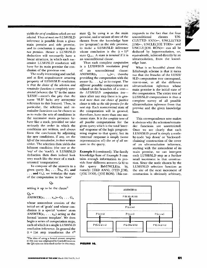
state Qt by using it as the main premise, and a variant of one of the clauses from the knowledge base (or 'program') as the side premise, to make a LUSH/SLD inference whose conclusion is the (t + 1) st state Qt+ 1. A state is terminal if it is an uncondit ional clause.

Thus each complete computation is a LUSH/SLD resolution proof

of an unconditional clause: ANSWER(tl . . . tm)<---, thereby providing the computation with the answer (tl . . . tm) as its output. The different possible computations are related as the branches of a t r ee - - the LUSH/SLD computation tree-- since after any step there is in general more than one choice of positive clause to take as the side premise for the next step. Each nonterminal state of the computation will in general, therefore, have more than one successor state. It is the complete tree of all possible computations for the given query which is the total 'inter- nal' response of the logic programming engine to that query; but its 'external ' response is simply (some representation of) the set of all answers to the query.

Example 5 (continued)• The family knowledge base of Example 5 contains enough information to provide four different answers (a b) to the query 3abUNCLE(a, b), namely: (TED ANN), (TED JIM), (JOE TOD), (JOE RON). This cor-

responds to the fact that the four uncondit ional clauses UN- CLE(TED ANN)*--, UNCLE(TED JIM)*-, UNCLE(JOE TOD)*- and UNCLE(JOE RON)*-- can all be deduced by hyperresolution, or, equivalently, inferred directly by an ultraresolution, from the knowledge base.

What is so beautiful about this Edinburgh scheme is that it turns out that the branches of the LUSH/ SLD computation tree correspond, one-to-one, to all the different ultraresolution inferences whose main premise is the initial state of the computation. The entire tree of LUSH/SLD computations is thus a complete survey of all possible ultraresolution inferences from that premise and the given knowledge base.

This correspondence now makes it obvious why the selection/remainder functions are unrestricted• Once we see clearly that each LUSH/SLD proof is simply a node- by-node 'top down' or 'backward- chaining' construction of the cover of an ultraresolution inference, starting with the antecedent of its main premise, we can interpret each LUSH/SLD step as a further small increment in that construction. Since the node chosen by the LUSH/SLD selection function as the site of the next increment of constuction is obviously arbitrary,

ANSWER (t) . . . . . . . . . . . . . . . . . . . . . . . . . . . . . . . . . . . . . . . . . . . .

P (K (t) t K (t))

P(uzw) . . . . . . . . . . . . . . . . . . . . . . . . . . . . . . . . . . . . . . . . . . . . . . . . . . . . . . . . . . . . . . . . . . . . . . . . . . . . . . . . . . . . . . .

P(xyu) P(yzv) P(xvw)

1 i I

F I G U R E 10.

C O M M U N I C A T I O N S O F T H E A C M / M a r c h 1 9 9 2 / V o 1 . 3 5 , N o , 3 61

L o g i c P r o g r a m m i n g there is no restriction on what that selection function is taken to be.

Serial vs. Parallel Computation in Logic Programming The branches of the LUSH/SLD computation tree in the first logic programming (Prolog) systems were generated serially, in a depth- first, backtracking search. This tree-search method is subject to embarrassing 'depth-first ' infinite runaways when nonterminat ing branches are present in the tree, but it is otherwise a simple, natural and effective way to search the complete LUSH/SLD computation tree and thus find the set of all answers to a query. The answers will be generated one at a time, as each terminal state is encountered. If a query has infinitely many answers (and the search tree therefore has infinitely many branches), then the set of all answers will simply (and correctly, in a reasonable sense) be generated as a nonterminat ing sequence.

It is surely clear, however, that the branches of the LUSH/SLD computation tree need not be con- structed one at a time in this depth- first back-tracking manner . One can instead grow the tree breadth- first, with no back-tracking, by computing successive sets of states, starting with the singleton set {Q0}, and continuing, in general, by comput ing the (t + 1) st set as the set of all the immediate successors of all the states in the t th set. The different completed computations, together with their associated answers, will be harvested, at each level, as their corresponding terminal states turn up in these state sets. There is, of course, no logical significance to the order in which these answers are generated: the answers logically form a set, not a sequence.

It is easy to find examples of queries which have infinitely many answers. For example, if the knowledge base is the set of clauses:

{NUMBER(0),.--, NUMBER(S(x)) ~---NUMBER(x)}

then the query ::Ix NUMBER(x) has

the set of answers:

{ x = 0 , x = s ( 0 ) , x = s ( s ( 0 ) ) . . . . . }.

Each answer comes from an ultraresolution inference whose main premise is:

ANSWER(x)~-NUMBER(x).

All these answers are given by covers which exhibit the same general pattern. The LUSH/SLD computation tree is an infinite binary tree which has only two states at each nonzero depth t. One of these two states is the clause

ANSWER(S(S(. . . 0.. .)))~---

with t occurrences of 's', and produces the answer

x = s ( s ( . . . 0 . . . ) ) ;

the other is the clause

ANSWER(S(S( . . . S ( x ) . . . ) ) ) ~--NUMBER(x)

with t + 1 occurrences of 's', which has two successors, and so on.

General Oueries and Answers Queries can contain universally quantified variables, and so can their answers. Consider, for example, the knowledge base:

P(u z w)~---P(x y u)P(y z v)P(x v w) P(x v w)*--P(x y u)P(y z v)P(u z w) P(G(a b) a b)*-- P(a H(a b) b*--.

and the query: 3 t Vk P(k t k). The negation of the query is: Vt 3k not P(k t k), so (as explained, for example, in [12]) in order to have a clause we must eliminate the existential quantifier. This is done by introducing a 'Skolem term' K(t) in place of the existential variable. The negated query then is: Vt not P(K(t) t K(t)), or in other words the negative clause: ~---P(K(t) t K(t)). Thus the initial state for the LUSH/ SLD computation is the clause: ANSWER(t)~--P(K(t) t K(t)).

An intuitive way to unders tand the clauses of this knowledge base is to interpret their variables as rang- ing over the elements of some set which is closed under a binary com- position opera t ion . , and to inter-

pret atoms P(a b c) as saying that a.b = c. The first two clauses then together assert that • is associative. The third says that the equation x.a = b always has the solution x = G(a b), while the fourth says that the equation a.x = b always has the solution x = H(a b). The query is then seen to be asking whether there is a t such that for all k, k-t = k, that is, whether there is a right identity element.

The kernel of the cover shown in Figure 10 is unifiable and has the mgu

c r = { t = z = H ( y y ) , x = G ( y K ( H ( y y ) ) ) , a = b = r = v = y , s = u = w = K ( H ( y y ) ) }

and so the inference yields the unconditional clause ANSWER(H(y y))*-- containing the universally quantified variable 'y'. In effect, the response to the query are there right identity elements? is the general proposition: yes--for all y, H(y y) is a right identity element.

Parallelism in Ultraresolution Inferences The potential parallelism in the breadth-first growth of the LUSH/ SLD tree is the kind which has come to be known as or-parallelism. Since each state may have several immediate-successor states it corresponds to the fact that there may be alternative possible choices of a positive clause as side premise for that state as main premise. As we have seen, the classical LUSH/SLD search (in its breadth-first version) is a clever way to compute all possible ultraresolution inferences which have a given conditional clause Q as main premise, with covering premises taken from a given fixed knowledge base P. So the or- parallel version of the LUSH/SLD process is a way of exploiting at least some of the potential parallelism of the uhraresolution inference scheme.

The challenge to the software and hardware designers of future logic programming systems, however, comes from the clear percep-

62 March 1992/Vol.35, No.3/COMMUNICATION$ OF THE ACM

tion that there is more potential parallelism 'waiting there' than just the or-parallelism. The computation of the set of all ultraresolutions with main premise Q and covering premises in P is abstractly just a matter of generating all covers of Q and then checking the kernel of each to see if it is unifiable. This, however, is precluded by a 'combinatorial explosion' problem. There are simply too many covers. Even in the small family knowledge base we considered earlier, there are (as we noted) only four ultraresolutions with the main premise

ANSWER(a b)*--UNCLE(a b)

and covering premises in the knowledge base. This means that there are only four covers of its antecedent whose kernels are unifiable. There are, however, several billion covers of this antecedent whose kernels are not unifiable. Despite the large size of the space to be searched in this simple example, a breadth-first (quasi-or-parallel) LUSH/SLD computation generates a tree of about 140 states, level by level down to a depth of about 25, in order to produce all four answers and to show that there are no more. The power of the LUSH/ SLD search method rests in the fact that entire subtrees of these 'fail- ures' are constantly being elimi- nated from the search. Its incremen- tal unification process in effect detects a source of nonunifiability as soon as it appears and therefore never permits a partially grown cover containing that 'lethal gene' to 'breed' any progeny at all. Thus the LUSH/SLD pruning of the tree is as drastic as it can be. Delaying any of this failure detection 'until later' will only allow these sources of failure to propagate multiplicatively, so that the future computational cost (whether in the extent of time consumed or in the number of parallel resources needed) of detecting all of them will grow at the same rate. Postponing all of the unification analysis until the generation of the set of all covers is completed

simply lets this effect maximize itself.

Here, however, it is clear that we have arrived at a point where merely logical considerations must yield the center stage to highly technical questions of algorithm design, complexity analysis, and parallel computation, the discussion of which is outside the scope of this article.

Glimpses Beyond In this article I have discussed only the historical and conceptual back- ground of the logical origins of logic programming. I have concentrated on the resolution theorem- proving ideas which have been my main interest from 1960 until the present. In describing its development to the present, I have briefly sketched the overall framework within which today's specialists are seeking to exploit as much as possible of the potential parallelism which is clearly present in the fun- damental processes. The rest of that story is now better left for others, more qualified, to tell.

Acknowledgments I am grateful to Jacques Cohen, Jack Minker and Jonas Barklund for their excellent suggestions after reading an earlier version of this article. I have tried to follow all of them. [ ]

References 1. Apt, K.R. and van Emeden, M.H.

Contributions to the Theory of Logic Programming. J. Assoc. Comput. Mach. 29 (1982), 841-862.

9. Barklund, J. Parallel unification. Ph.D. thesis, Computing Science Department, Uppsala University, 1990.

3. Baxter, L.D. An efficient unification algorithm. Tech. Rep. CS-73- 23, Department of Computer Sci- ence, University of Waterloo, 1973.

4. Baxter, L.D. The complexity of unification. Ph.D. thesis, University of Waterloo, 1976.

5. Boyer, R.S. and Moore, J.S. The Sharing of Structure in Theorem Proving Programs. Mach. lntell. 7 (1972), 101-116.

6. Church, A. A note on the

entscheidungsproblem. J. Symbolic Logic 1 (1936) 40-41. (Reprinted in [11]).

7. Colmerauer, A. Les Systemes-Q ou un formalisme pour analyser et syn- thesizer des phrases sur ordinateur. Rep. 43, Department of Computer Science, University of Montreal, 1970.

8. Colmerauer, A., Kanoui, H., Pasero, R. and Roussel, P. Un sys- teme de communication homme- machine en Frangais. Tech. Rep., Groupe d'Intelligence Artificielle, Universite d'Aix Marseille II, Luminy, France, 1973.

9. Davidon, W. Personal communication, 1962.

10. Davis, M. Eliminating the irrelevant from mechanical proofs. In Proceed- ings, Symposia of Applied Mathematics 15, American Mathematical Society, 1963, pp. 15-30. (Reprinted in [44], vol. 1, 315-330).

11. Davis, M., Ed. The Undecidable: Basic Papers on Undecidable Propositions, Unsolvable Problems, and Computable Functions. Raven Press, 1965.

12. Davis, M. and Putnam, H. A computing procedure for quantification theory. J. Assoc. Comput. Mach. 7 (1960), 201-216. (Reprinted in [44], vol. 1, 125-139).

13. Dwork, C, Kanellakis, P., and Mitchell, J.C. On the sequential nature of unification.J. Logic Program. 1, (1984), 35-50.

14. Frege, G. Begriffsschrifft, a Formula Language, Modelled Upon that of Arithmetic, for Pure Thought. English translation in [48], 1-82.

15. Gentzen, G. The Collected Papers of Gerhard Gentzen. M.E. Szabo Ed., North-Holland, 1969.

16. Gilmore, P.C. A Proof Method for Quantification Theory: its Justifica- tion and Realization. IBM J. Res. Dev. 4 (1960), 28-35. (Reprinted in [44], volume 1, 151-158).

17. GOdel, K. The Completeness of the Axi- oms of the Functional Calculus of Logic, 1930. English translation, with commentary, in [48], 582-291.

18. Green, C.C. The application of theorem-proving to problem solving. In Proceedings of the first International Joint Conference on Artificial Intelli- gence (Washington, D.C., 1969), pp. 219-240.

19. Herbrand, J. Investigations in Proof Theory (1930). English translation of main parts, with commentary, in [48], 525-581, and of entire thesis in Jacques Herbrand: Logical Writings

COMMUNICATIONS OF THE ACM/March 1992/Vo1.35, No.3 63

L o g i c P r o g r a m m i n g

(edited by Warren Goldfarb), Har- vard, 1971, 44-202.

20. Hewitt, C. PLANNER: A language for proving theorems in robots. In Pro- ceedings of the first International Joint Conference on Artificial Intelligence, (Wash., D.C., 1969), pp. 295-301.

21. Hill, R. LUSH Resolution and its Completeness. DCL Mem. 78, De- partment of Artificial Intelligence, University of Edinburgh, 1974.

22. Huet, G. Resolution des equations dans langages d'order 1, 2 . . . . oJ. These d'Etat, Universite Paris VII, 1976.

23. Kneale, W.C. and Kneale, M. The Development of Logic. Oxford, 1962.

24. Kowalski, R.A. Predicate Calculus as a Programming Language. In Proceedings of Sixth IFIP Congress, North Holland, 1974, pp. 569-574.

25. Kowalski, R.A. Logic for Problem Solving. North-Holland, 1979.

26. Kowalski, R.A. The early years of logic programming. Commun. ACM 31 (1988), 38-43.

27. Kowalski, R.A. and Kuehner, D. Linear Resolution with Selection Func- tion. Artificial Intelligence 2 (1971), 227-260. (Reprinted in [44], volume 1, 542-577).

28. Loveland, D.W. Mechanical theorem proving by model elimination. J. ACM 15 (1968), 236-251. (Re- printed in [44], volume 2, 117- 134).

29, L6wenheim, L. On Possibilities in the Calculus of Relatives, 1915. English translation in [48], 228-251.

30. Luckham, D. Refinement Theorems in Resolution Theory. Lecture Notes in Mathematics 125, Springer, 1970, 163-190.

31. McCarthy, J. Programs with Com- mon Sense. In Proceedings of a Sym- posium on the Mechanization of Thought. H.M. Stationery Office, London, 1959. (Reprinted in Se- mantic Information Processing MIT Press, 1968).

32. Minsky, M. The Society of Mind. Simon and Schuster, 1985.

33. Newell, A., Shaw, J.C. and Simon, H.A. Empirical explorations with the logic theory machine: A case study in heuristics. In Proceedings of the Western Joint Computer Conference (1957), pp. 218-239. (Reprinted in [44], volume 1, 49-73).

34. Prawitz, D. An Improved Proof Proce- dure. Theori_a 26 (1960) 102-139. (Reprinted in [44], volume 1, 159- 199, with a preface by the author).

35. Prawitz, D., Prawitz, H. and

Voghera, N. A mechanical proof procedure and its realization in an electronic computer.JACM 7 (1960) 102-128. (Reprinted in [44], volume 1, 200-228).

36. Raphael, B. Programming a robot. In Proceedings of Fourth IFIP Con- gress, North Holland, 1968, 135- 139.

37. Robinson, A. Proving a theorem (as Done by Man, Logician, or Ma- chine). Summaries of talks presented at the Summer Institute for Symbolic Logic. Communications Research Division, Institute for Defense Analysis, Princeton, 1957. (Reprinted in [44], volume 1, 74- 76).

38. Robinson, J.A. Theorem proving on the computer. J. Asso. Comput. Mach. 10 (1963) 163-174. (Re- printed in ]44], volume 1, 372- 383).

39. Robinson, J.A. A machine-oriented logic based on the resolution principle. JACM 12 (1965), 23-41. (Re- printed in [44], volume 1, 397- 415).

40. Robinson, J.A. Automatic Deduc- tion with Hyper-resolution. Int. J. Comput. Math. 1 (1965), 227-234. (Reprinted in [44], volume 1 ,416- 423).

41. Robinson, J.A. Computational logic: the unification computation. Machine Intell. 6 (1970), 63-72.

42. Robinson, J.A. Fast Unification. Tagung fiber Automatisches Be- weisen, Mathematisches For- schungsinstitut Oberwolfach, 1976.

43. Robinson, G.A. and Wos, L.T. Paramodulation and theorem proving in first-order theories with equality. Machine lntell. 4 (1969), 103-133.

44. Siekmann, J.H. and Wrightson, G. Eds. Automation of Reasoning. Classi- cal Papers on Computational Logic (1957-1966). Two volumes, Springer, 1983.

45. Skolem, T. Logico-combinatorial In- vestigations in the Satisfiability or Provability of Mathematical Proposi- tions (1920). English translation, with commentary, in [48], 252-263.

46. Tarski, A. Logic, Semantics, Metamathematics: Papers from 1923 to 1938, translated by J.H. Woodger, Oxford, 1956.

47. Turing, A.M. On computable numbers, with an application to the entscheidungsproblem. In Proceed- ings of the London Mathematical Soci- ety, 1937. (Reprinted in l l 1]).

48. van Heijenoort, J. Ed. From Frege to Godel; A Source Book in Mathematical Logic, 1879-1931. Harvard Univer- sity Press, 1967.

49. Wang, H. Towards mechanical mathematics. IBM J. Res. Dev. 4 (1960), 2-22. (Reprinted in [44], volume 1, 244-264).

50. Warren, D.H.D. Implementing PROLOG--compiling predicate logic programs (Res. Rep. 39 and 40), and Logic programming and compiler writing (Res. Rep. 44). Department of Artificial Intelli- gence, University of Edinburgh, 1977.

51. Winograd, T. Understanding Natural Language. Academic Press, 1973.

52. Wos, L.T., Carson, D. and Robin- son, G.A. The unit preference strategy in theorem proving. AF1PS Conference Proceedings 26, Spartan Books, Wash. D.C., 1964, pp. 615- 621. (Reprinted in [44], vol. 1 ,387- 393).

53. Wos, L.T., Carson, D. and Robin- son, G.A. Efficiency and completeness of the set of support strategy in theorem proving. J. Assoc. Comput. Mach. 12, 1965, pp. 536-541, (Re- printed in [44], volume 1, 484- 489).

CR Categories and Subject Descrip- tors: D. 1.6 [Programming Techniques]: Logic Programming; D.3.2 [Program- ming Languages]: Language Classifica- tions--PROLOG; F.2.2 [Analysis of Algorithms and Problem Complexity]: Nonnumerical Algorithms and Prob- lems--complexity of proof procedures, pattern matching; F.4.1 [Mathematical Logic and Formal Languages]: Mathematical Logic--computational logic, logic programming, mechanical theorem proving, proof theory; 1.2.3 [Artificial Intelligence]: Deduction and Theorem Proving-- answer~reason extraction, deduction, logic programming, metatheory, resolution; 1.2.4 [Artificial Intelligence]: Knowledge Representation Formalisms and Methods--predicate logic

Additional Key Words and Phrases: Unification

Further Reading Several excellent a n d recent fur-

ther sources are: J.W. Lloyd's Foundations of Logic Programming (second, ex t ended edit ion, Spr inger -Ver lag 1987) and Logic,

64 March 1992/Vo1.35, No.3/COMMUNICATIONS OF THE ACM

Programming and Prolog by Ulf Nils- son and Jan Maluszynski (Wiley, 1990) provide r igorous but reada- ble accounts not only of much of the material covered in the present article but also of many noteworthy later developments. Among these are:

• the addit ion of imperative con- trol features such as the cut;

• the elegant negation as failure technique by which all modern Prolog systems permit negative conditions in both positive and negative conditional clauses;

• the inclusion of arithmetical, list- processing, metalinguistic and other appl ied predicates and operators among the atoms and terms;

• alternative logic p rogramming paradigms, such as concurrent logic programming, constraint logic programming, and higher-order logic programming.

For the reader who wishes to learn more about applications and methodology of logic programming, about Prolog, and about exploit ing the potential parallelism in logic, I also recommend the following recent books:

• The Art of Prolog by L. Sterling and E. Shapiro (MIT Press, 1986);

• Prolog Programming for Artificial Intelligence by I. Bratko (second edition, Addison-Wesley, 1990);

• The Craft of Prolog by R. O'Keefe (MIT Press, 1990).

• Essentials of Logic Programming by C.J. Hogger (Oxford: Clarendon Press, 1990),

• Parallelism in Logic: its potential for performance and program development by Franz Kurfess (Braun- schweig, Vieweg, 1991).

• Parallel Logic Programming by Evan Tick (MIT Press, 1991).

About the Author: J.A. ROBINSON teaches philosophy and computer science at the University of Syracuse, where he is now University Professor. His research interests include computational logic and automated deduction. He is currently working on a massively parallel logical computation

system combining the lambda calculus (for functional programming) with the predicate calculus (for logic programming) at the University of Tokyo, where he is on a year's leave. Author's Present Address: Office of the University Pro- fessor, Syracuse University, Syracuse, NY 13244-2010 Permission to copy without fee all or part of this material is granted provided that the

copies are not made or distributed for direct commercial advantage, the ACM copyright notice and the title of the publication and its date appear, and notice is given that copying is by permission of the Association for Computing Machinery. To copy otherwise, or to republish, requires a fee and/or specific permission.

© ACM 0002-0782/92/0300-040 $1.50

ALS Prolog realizes Logic Programming.

Logic Programming provides one of the most advanced and refined approaches ~ f o r solving complex programming problems. After all, L ~ 7 / logic itselfhas been under development by the human race ~ - . J ~ for well over 2,000 years. Prolog is the most successful ~ , ._~/ realization of the Logic Programming approach, providing/""--~ a very high conceptual approach to problem analysis and implementation, coupled with extremely general and fast pattern-matching.//~-~ And ALS Prolog is by far the most powerful collection o f \ ~ f ~ \ Prolog compilers available. Whether your task is ~ / ~ advanced exploratory research, or the development of ~ complex production systems, the ALS Prolog compiler is the ~ I tool of choice. Develop with one ALS Prolog compiler, and you re developing with them all. ALS is committed to a uniform implementation

all platforms, yet you get access to all ~ the facilities of on each platform, including each native win- ~ . ~ / dowing system. You can couple your Prolog programs to C ~ programs via a very broad C interface ~ which allows Prolog to manipulate C data, and allows C to \ ~ / ~ c a l l into Prolog. Stream-based IPC communication, l o c a l k ~ / / a n d remote, is available. We support 386/486 machines under SCO Unix and DOS (virtual memory), soon with Windows 3.0, as well as the Apple ~ Macintosh, Sun SPARC and 680x0, DEC v a x (VMS) and ~ 7 ~ ~ all Motorola 88000-based machines, and planning to add even more platforms in the future. ~ ~ j ~ Z ~ ~ ] ~ [ Call or write today. If you're learning Prolog, ask about our student versions l l APPLIED LOGIC SYSTEMS, INC. for the PC and ~ P.O. BOX 90, UNIVERSITY STATION Macintosh. 1 1 SYRACUSE, NY, 13210 USA

1 PHONE: 315-471-3900 FAX:315-471-2606

Circle #79 on Reader Service Card

COMMUNICATIONS OF THE ACM/March 1992/Vol.35, No.3 6 S

logic and logic programming - department of computer science · 2016-08-18 · logic programming...

Documents