Log property mapping guided with seismic attributes Edgar Galvan Aguilar Geophysicist Schlumberger eaguilar@slb.com

1. Introduction

The integration of seismic data with other geological data has provided not only the accurate

subsurface imaging but also an apt description, both the variations in the physical properties of

the rocks as the fluid content. The integrated approach of interpretation has greatly reduced the

risk associated with drilling of wells in existing fields and hence improved the efficiency and life

of producing reservoirs. This has become possible only with the extensive use of seismic

attributes integrating with log properties for reservoir characterization.

Known the distribution of porosity in the subsurface, is essential for the generation of leads. The

integration of seismic attributes with petrophysical measurements from wells can significantly

improve the spatial distribution of log properties.

This paper is an attempt to estimate the porosity distribution in the study area using two

dimensional geostatistical methods in GeoFrame 4.5 using ResSum to compute average

reservoir properties and LPM to map the properties guided by seismic attributes. After

structural mapping various attribute maps have been generated from the 3-D seismic data

volume. The linear regression through least square fit was established between window based

seismic amplitude attribute and effective porosity. This relation has been used to generate the

effective porosity maps for Top Paris reservoir sand. The Cloudspin dataset was used to develop

this workflow, the study area falls in North Gulf of Mexico basin.

2. Workflow

GeoFrame 4.5 was used for the full workflow; modules used include LPM, ResSum, WellPix,

Charisma, Synthetics and GF Basemap.

This project is divided in 3 stages:

Geological Interpretation. Reservoir top and base interpretation and layer definition

(WellPix).

Seismic Interpretation. Seismic horizon correlation and seismic attributes generation

(Charisma).

Reservoir property mapping. Summation model setup, cutoff definition and reservoir

properties mapping (ResSum and LPM).

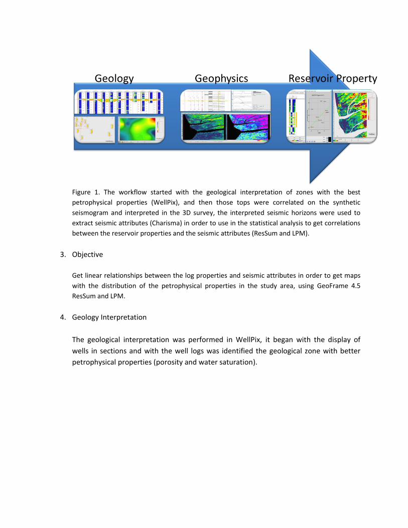
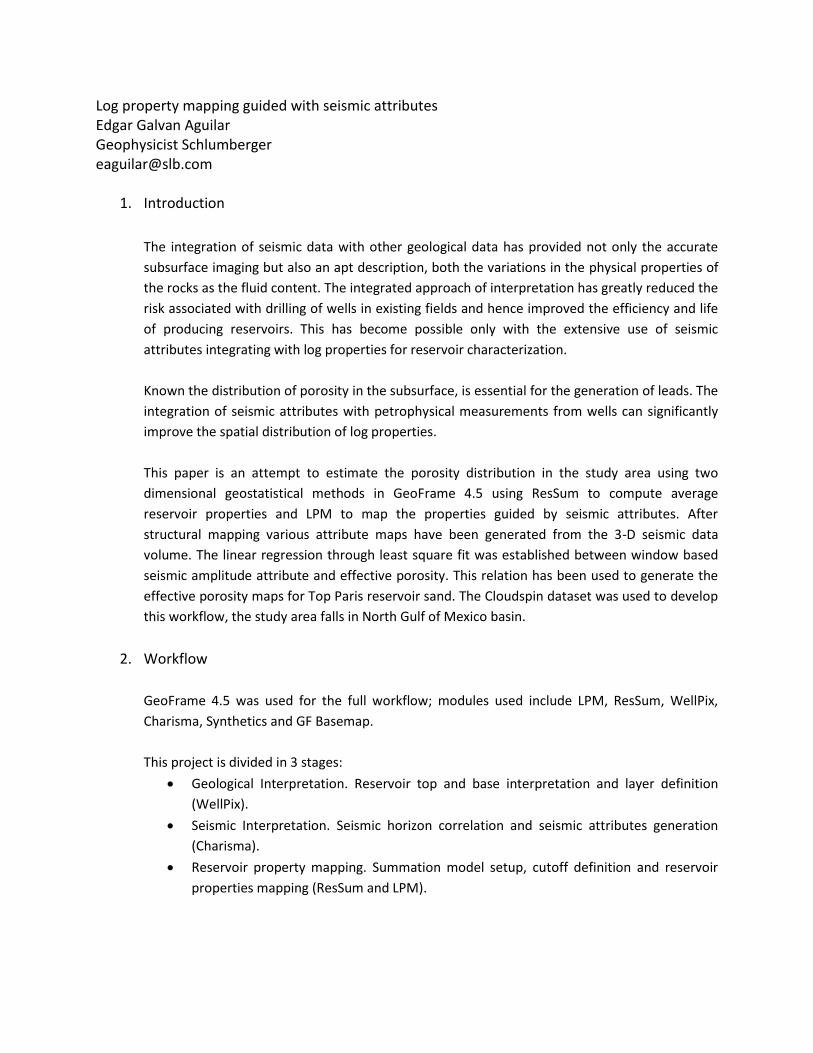
Figure 1. The workflow started with the geological interpretation of zones with the best

petrophysical properties (WellPix), and then those tops were correlated on the synthetic

seismogram and interpreted in the 3D survey, the interpreted seismic horizons were used to

extract seismic attributes (Charisma) in order to use in the statistical analysis to get correlations

between the reservoir properties and the seismic attributes (ResSum and LPM).

3. Objective

Get linear relationships between the log properties and seismic attributes in order to get maps

with the distribution of the petrophysical properties in the study area, using GeoFrame 4.5

ResSum and LPM.

4. Geology Interpretation

The geological interpretation was performed in WellPix, it began with the display of

wells in sections and with the well logs was identified the geological zone with better

petrophysical properties (porosity and water saturation).

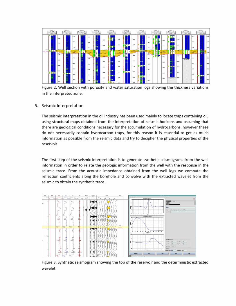
Figure 2. Well section with porosity and water saturation logs showing the thickness variations

in the interpreted zone.

5. Seismic Interpretation

The seismic interpretation in the oil industry has been used mainly to locate traps containing oil,

using structural maps obtained from the interpretation of seismic horizons and assuming that

there are geological conditions necessary for the accumulation of hydrocarbons, however these

do not necessarily contain hydrocarbon traps, for this reason it is essential to get as much

information as possible from the seismic data and try to decipher the physical properties of the

reservoir.

The first step of the seismic interpretation is to generate synthetic seismograms from the well

information in order to relate the geologic information from the well with the response in the

seismic trace. From the acoustic impedance obtained from the well logs we compute the

reflection coefficients along the borehole and convolve with the extracted wavelet from the

seismic to obtain the synthetic trace.

Figure 3. Synthetic seismogram showing the top of the reservoir and the deterministic extracted

wavelet.

This extracted wavelet gives us information about the frequencies in the extraction window as

well as information about the polarity and phase of the seismic data. After obtaining the

synthetic trace, we use the well tops to observe the seismic response of geologic top at this

stage to define the seismic horizons interpreted in 3D Studio.

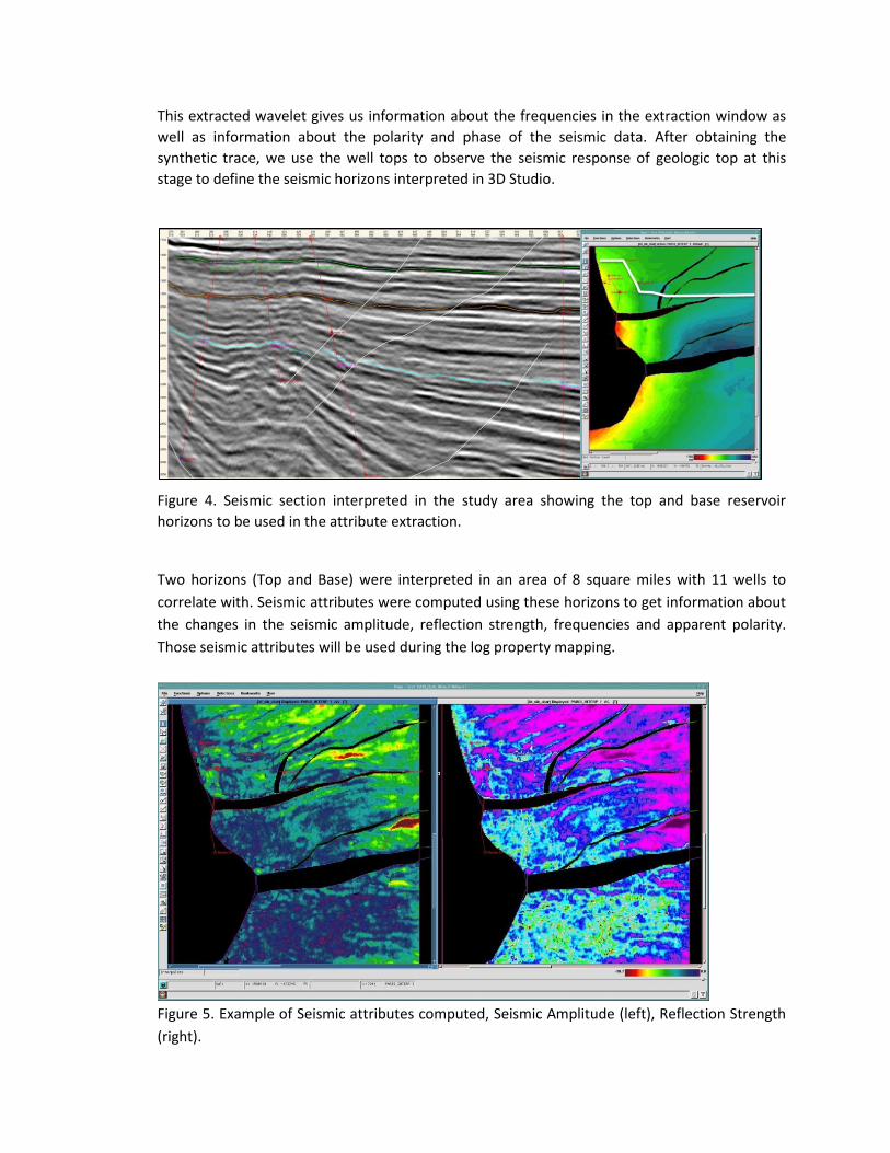
Figure 4. Seismic section interpreted in the study area showing the top and base reservoir

horizons to be used in the attribute extraction.

Two horizons (Top and Base) were interpreted in an area of 8 square miles with 11 wells to

correlate with. Seismic attributes were computed using these horizons to get information about

the changes in the seismic amplitude, reflection strength, frequencies and apparent polarity.

Those seismic attributes will be used during the log property mapping.

Figure 5. Example of Seismic attributes computed, Seismic Amplitude (left), Reflection Strength

(right).

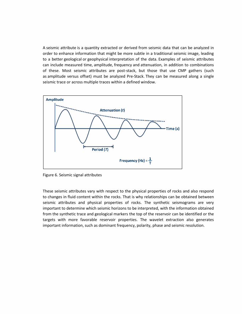
A seismic attribute is a quantity extracted or derived from seismic data that can be analyzed in

order to enhance information that might be more subtle in a traditional seismic image, leading

to a better geological or geophysical interpretation of the data. Examples of seismic attributes

can include measured time, amplitude, frequency and attenuation, in addition to combinations

of these. Most seismic attributes are post-stack, but those that use CMP gathers (such

as amplitude versus offset) must be analyzed Pre-Stack. They can be measured along a single

seismic trace or across multiple traces within a defined window.

Figure 6. Seismic signal attributes

These seismic attributes vary with respect to the physical properties of rocks and also respond

to changes in fluid content within the rocks. That is why relationships can be obtained between

seismic attributes and physical properties of rocks. The synthetic seismograms are very

important to determine which seismic horizons to be interpreted, with the information obtained

from the synthetic trace and geological markers the top of the reservoir can be identified or the

targets with more favorable reservoir properties. The wavelet extraction also generates

important information, such as dominant frequency, polarity, phase and seismic resolution.

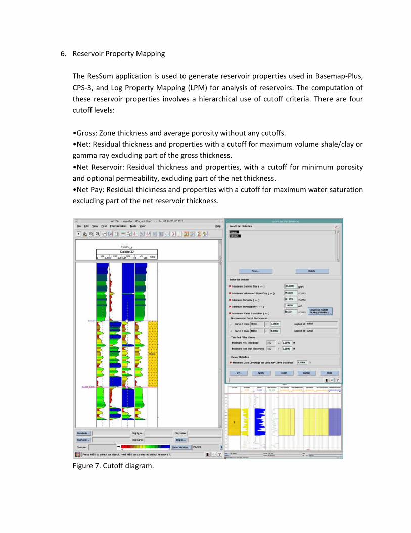
6. Reservoir Property Mapping

The ResSum application is used to generate reservoir properties used in Basemap-Plus,

CPS-3, and Log Property Mapping (LPM) for analysis of reservoirs. The computation of

these reservoir properties involves a hierarchical use of cutoff criteria. There are four

cutoff levels:

•Gross: Zone thickness and average porosity without any cutoffs.

•Net: Residual thickness and properties with a cutoff for maximum volume shale/clay or

gamma ray excluding part of the gross thickness.

•Net Reservoir: Residual thickness and properties, with a cutoff for minimum porosity

and optional permeability, excluding part of the net thickness.

•Net Pay: Residual thickness and properties with a cutoff for maximum water saturation

excluding part of the net reservoir thickness.

Figure 7. Cutoff diagram.

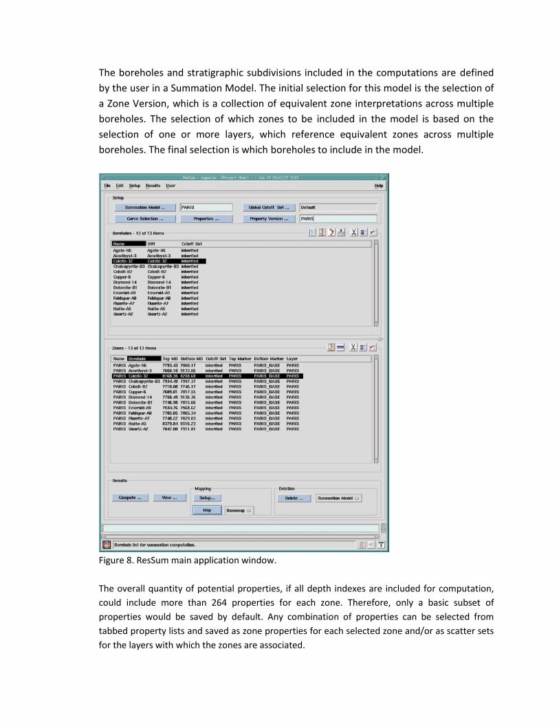
The boreholes and stratigraphic subdivisions included in the computations are defined

by the user in a Summation Model. The initial selection for this model is the selection of

a Zone Version, which is a collection of equivalent zone interpretations across multiple

boreholes. The selection of which zones to be included in the model is based on the

selection of one or more layers, which reference equivalent zones across multiple

boreholes. The final selection is which boreholes to include in the model.

Figure 8. ResSum main application window.

The overall quantity of potential properties, if all depth indexes are included for computation,

could include more than 264 properties for each zone. Therefore, only a basic subset of

properties would be saved by default. Any combination of properties can be selected from

tabbed property lists and saved as zone properties for each selected zone and/or as scatter sets

for the layers with which the zones are associated.

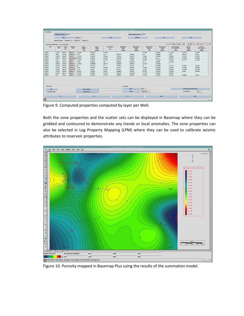
Figure 9. Computed properties computed by layer per Well.

Both the zone properties and the scatter sets can be displayed in Basemap where they can be

gridded and contoured to demonstrate any trends or local anomalies. The zone properties can

also be selected in Log Property Mapping (LPM) where they can be used to calibrate seismic

attributes to reservoir properties.

Figure 10. Porosity mapped in Basemap Plus using the results of the summation model.

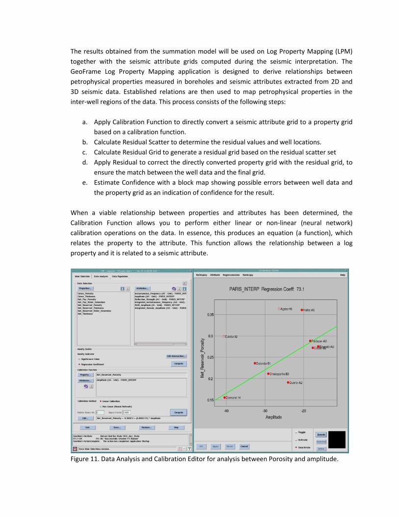
The results obtained from the summation model will be used on Log Property Mapping (LPM)

together with the seismic attribute grids computed during the seismic interpretation. The

GeoFrame Log Property Mapping application is designed to derive relationships between

petrophysical properties measured in boreholes and seismic attributes extracted from 2D and

3D seismic data. Established relations are then used to map petrophysical properties in the

inter-well regions of the data. This process consists of the following steps:

a. Apply Calibration Function to directly convert a seismic attribute grid to a property grid

based on a calibration function.

b. Calculate Residual Scatter to determine the residual values and well locations.

c. Calculate Residual Grid to generate a residual grid based on the residual scatter set

d. Apply Residual to correct the directly converted property grid with the residual grid, to

ensure the match between the well data and the final grid.

e. Estimate Confidence with a block map showing possible errors between well data and

the property grid as an indication of confidence for the result.

When a viable relationship between properties and attributes has been determined, the

Calibration Function allows you to perform either linear or non-linear (neural network)

calibration operations on the data. In essence, this produces an equation (a function), which

relates the property to the attribute. This function allows the relationship between a log

property and it is related to a seismic attribute.

Figure 11. Data Analysis and Calibration Editor for analysis between Porosity and amplitude.

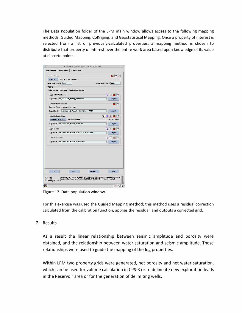
The Data Population folder of the LPM main window allows access to the following mapping

methods: Guided Mapping, CoKriging, and Geostatistical Mapping. Once a property of interest is

selected from a list of previously-calculated properties, a mapping method is chosen to

distribute that property of interest over the entire work area based upon knowledge of its value

at discrete points.

Figure 12. Data population window.

For this exercise was used the Guided Mapping method; this method uses a residual correction

calculated from the calibration function, applies the residual, and outputs a corrected grid.

7. Results

As a result the linear relationship between seismic amplitude and porosity were

obtained, and the relationship between water saturation and seismic amplitude. These

relationships were used to guide the mapping of the log properties.

Within LPM two property grids were generated, net porosity and net water saturation,

which can be used for volume calculation in CPS-3 or to delineate new exploration leads

in the Reservoir area or for the generation of delimiting wells.

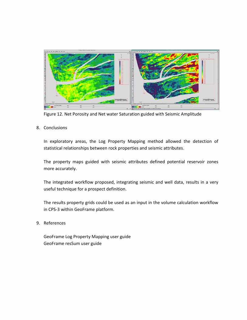
Figure 12. Net Porosity and Net water Saturation guided with Seismic Amplitude

8. Conclusions

In exploratory areas, the Log Property Mapping method allowed the detection of

statistical relationships between rock properties and seismic attributes.

The property maps guided with seismic attributes defined potential reservoir zones

more accurately.

The integrated workflow proposed, integrating seismic and well data, results in a very

useful technique for a prospect definition.

The results property grids could be used as an input in the volume calculation workflow

in CPS-3 within GeoFrame platform.

9. References

GeoFrame Log Property Mapping user guide

GeoFrame resSum user guide