location choice in two-sided markets with indivisible agents

Games and Economic Behavior 69 (2010) 2–23www.elsevier.com/locate/geb

Location choice in two-sided markets with indivisible agents ✩

Robert M. Anderson a, Glenn Ellison b, Drew Fudenberg c,∗

a University of California, Berkeley, USAb Massachusetts Institute of Technology, USA

c Harvard University, USA

Received 5 December 2006

Available online 8 May 2008

Abstract

Consider a model of location choice by two sorts of agents, called “buyers” and “sellers”: In the first period agents simultaneouslychoose between two identical possible locations; following this, the agents at each location play some sort of game with the otheragents there. Buyers prefer locations with fewer other buyers and more sellers, and sellers have the reverse preferences. We studythe set of possible equilibrium sizes for the two markets, and show that two markets of very different sizes can co-exist even iflarger markets are more efficient. This extends the analysis of Ellison and Fudenberg [2003. Quart. J. Econ. 118, 1249–1278],who ignored the constraint that the number of agents of each type in each market should be an integer, and instead analyzed the“quasi-equilibria” where agents are treated as infinitely divisible.© 2008 Elsevier Inc. All rights reserved.

JEL classification: C62; L14; O18; R11

Keywords: Agglomeration; Two-sided markets; Quasi-equilibrium; Tipping; Large finite economies; Integer constraints; Indivisibility;Nonstandard analysis

1. Introduction

In many economic models, agents benefit from interactions with agents whose characteristics are in some waydifferent than their own. In exchange economies, agents gain from interactions with agents whose endowments orpreferences are different; in economies with production, gains come about when producers interact with consumers,and in opposite-sex marriage “markets” gains arise from men meeting women. Many of these activities seem to beagglomerated: for example many industries are geographically concentrated, and trade in many goods takes place ina small number of marketplaces.

One explanation in the literature for the observed levels of agglomeration is that the agglomeration arises from“tipping” in the presence of increasing returns to scale. In the simplest such model, there is a continuum of identical

✩ This work was supported by NSF grants SES-0214164, SES-0219205, SES-0112018, and SES-0426199 and by the Coleman Fung Chair inRisk Management at UC Berkeley.

* Corresponding author at: Harvard University, Department of Economics, Cambridge, MA, USA.E-mail addresses: [email protected] (R.M. Anderson), [email protected] (G. Ellison), [email protected] (D. Fudenberg).

0899-8256/$ – see front matter © 2008 Elsevier Inc. All rights reserved.doi:10.1016/j.geb.2008.04.009

R.M. Anderson et al. / Games and Economic Behavior 69 (2010) 2–23 3

agents, who all prefer to be part of the largest market: Here the only equilibria are for all active markets to be the samesize, and the only stable equilibria assign all of the agents to the same location. More strongly, these agglomeratedor “completely tipped” outcomes are the only equilibria in models with a finite number of agents: The equal-market-shares outcomes are not equilibria when the agents have finite size, as a shift by a single agent makes the agent’s newmarket larger and hence better than the one she left.

However, in many cases of interest, agents are not identical, and while all agents prefer larger markets, they alsoprefer markets with few agents of their own type, so that e.g. the buyer–seller ratio is more favorable. In this case, anagent who switches markets has an adverse “market impact” effect on the market she joins. When a seller contemplatesa switch from market 1 to market 2, she should take into account that her joining market 2 will increase the seller–buyer ratio there, and thereby makes that market less attractive for all sellers, including herself. This raises the questionof whether the market impact effect can generate equilibria with several active markets, or whether we should expectactivity to concentrate in a single market absent any diseconomies (such as transportation costs) from doing so. Thisquestion cannot be resolved by working only with a continuum model, as often both the market impact effect and thebenefits of agglomeration vanish as the market size becomes infinite. Instead, we study a model of location choice ina finite population composed of two sorts of agents, whom we will call “buyers” and “sellers.”

The structure of the model is the same as in Ellison and Fudenberg (2003): In the first period of the model, agentssimultaneously choose between two identical possible locations or markets. Following this, the agents at each locationplay some sort of game with the other agents there; the resulting payoffs are determined by the numbers of each typeof agent who chose the same location.1 We suppose that buyers prefer markets with fewer other buyers and moresellers, and that sellers have the reverse preferences. Thus, when the numbers of buyers and sellers are even, there isan equilibrium where the two markets are exactly the same size.2

The traditional view (see e.g. Krugman, 1991b) was that outcomes with two or more active markets are an unstableknife-edge whenever there are increasing returns, that is when larger markets are more efficient. Ellison and Fudenberg(2003) show that this view is incorrect, and that the “market impact effect” can allow several markets to remain open inequilibrium: instead of split market outcomes being an unstable knife-edge, there can be a “plateau” of such equilibria.As noted above, both the market impact effect and the benefit of increasing returns often vanish as the number ofagents in each market grows to infinity. Ellison and Fudenberg (2003) argue that in many models of interest the effectsvanish at the same rate. When this is true, Ellison and Fudenberg show that the incentive constraints for equilibriumare consistent with two large markets being active even when their sizes are unequal, and they give a lower bound onthe width of this plateau. However, they ignore the constraint that the number of agents of each type in each marketshould be an integer, and instead analyze the “quasi-equilibria” in which agents are treated as infinitely divisible. Forthis reason, Ellison and Fudenberg’s (2003) results say nothing about the existence of exact equilibria—outcomes thatsatisfy all of the incentive constraints and also assign an integer number of agents of each type to each market.

In the context of competing auction sites, Ellison et al. (2004) show that when the number of buyers is largeand buyer values are uniformly distributed, for any quasi-equilibrium size ratio α of the game with B buyers and S

sellers, there is a nearby S′ for which the game with B buyers and S′ sellers has an exact equilibrium with size ratioapproximately α. This shows that exact equilibria exist in some large economies, but says nothing about the number ofequilibria for a typical pair (S,B). Indeed, it leaves open the possibility that most pairs (S,B) have no exact equilibriaother than complete tipping.

The point of this paper is to complete the analysis of tipping in large markets by providing a thorough analysis ofequilibrium, paying attention to the constraint that each agent is indivisible. Put briefly, we have four main findingsabout economies (payoff functions and aggregate seller–buyer ratios) that satisfy the Ellison and Fudenberg (2003)assumptions.

1 The assumption that buyers and sellers move simultaneously is most natural when the agents on the two sides of the market are roughlysymmetric; some cases might be better described by asymmetric models where all the sellers move before any of the buyers. Note also that ourmodel does not consider any actions by market makers such as eBay.

2 More precisely, our results imply that when the numbers of buyers and sellers are even and sufficiently large, there is an equilibrium where thetwo markets are exactly the same size. We expect that typically this equilibrium will also be present even when the numbers of buyers and sellersis small, but have not tried to provide precise conditions under which this is true.

4 R.M. Anderson et al. / Games and Economic Behavior 69 (2010) 2–23

1. We sharpen the Ellison and Fudenberg (2003) result on quasi-equilibria by giving an upper bound on the size ofthe two-market plateau and a sharper lower bound. As S and B grow,3 these bounds converge, so that in the limitwe have a necessary and sufficient condition.

2. Under some natural specifications of payoffs there are sequences {Sn,Bn} with Bn → ∞ that completely tip forall n. That is, at each point in the sequence, the only pure strategy equilibria are the ones in which all agentschoose the same location, so the plateau of two-market equilibria is empty.Despite the finding in point 2, it turns out that the sequences along which two-market equilibria fail to exist arequite special. Specifically,

3. For any ε > 0, there is a bound M such that if the aggregate buyer–seller and seller–buyer ratios are at least ε

away from every integer, and the number of agents is at least M , then there is a range of exact equilibria. Forfixed payoff functions the width of this range (expressed in terms of the proportion of agents in each market) isindependent of the number of buyers and sellers when these are large.

4. Moreover, for generic sequences {Sn,Bn} with Bn → ∞ and Sn/Bn convergent, there is a plateau of exact equi-libria for all large n. This plateau includes all of the size ratios predicted by the Ellison and Fudenberg (2003)result, and typically includes others as well. Moreover, the density of equilibria (i.e. the proportion of integers ina given range such that there is an equilibrium with that many buyers in one market, and the rest in the other)converges to a specific piecewise-linear function that we identify. When there are fewer buyers than sellers, foralmost all integer numbers of buyers in the center of the plateau, there is an equilibrium with that many buyers inmarket 1; the symmetric statement is true when there are more buyers than sellers.

The reason that the result in point 1 delivers more size ratios than Ellison and Fudenberg (2003) is that their resultprovided a condition for the incentive constraints to be satisfied with exactly the same seller–buyer ratio in eachmarket. The proof of the new result, like the Ellison et al. (2004) characterization of the quasi-equilibrium set in thecase of uniformly distributed buyer values, allows the seller–buyer ratios in the two markets to be slightly unequal,which in some cases leads to a substantially larger range of size ratios.

The plateau of equilibria characterized in point 4 exists generically because it obtains whenever Sn/Bn has anirrational limit. Since the set of rational numbers has measure 0, our genericity result is analogous to the formulationof a generic sequence of purely competitive economies in, for example, Grodal (1975) and Dierker (1975). The reasonthat sequences with an irrational limit are better behaved is closely related to the fact that the map that sends x to(x +y)mod 1 is an ergodic transformation if and only if y is irrational. Fix a model with S sellers and B buyers overall,and let γ = S/B . Whether there is an equilibrium with an integer B1 of buyers in market 1 depends on whether thereis an integer S1 satisfying certain inequalities. This in turn depends on whether (γB1)mod 1 lies in a certain intervalin [0,1], where the length of the interval is the piecewise linear function of α = B1/B referred to above. When B islarge, the piecewise linear function changes slowly in response to changes in B1, while (γB1)mod 1 has, by ergodicity,essentially the uniform distribution on [0,1]. Consequently, the density of the set of integers B1 such that (γB1)mod 1lies in the interval converges to the length of the interval.

Another way to formulate the characterization in point 4 is as a statement about the probability that a randomlychosen large economy will have a broad plateau of equilibria with equilibria spread throughout it with the density H

that we define. We show that if a sequence of economies is chosen at random by choosing some sequence {Bn} withBn → ∞ and then choosing Sn to match as closely as possible a seller–buyer ratio drawn from some density functionon a compact support, then the probability that the nth economy has a large plateau of equilibria with an equilibriumdensity that is within ε of H goes to one as n → ∞.

The result in point 4 is proved using nonstandard analysis, which is a way of formalizing and manipulating infinites-imal, and infinitely large, quantities. The statement of the result, however, is entirely standard and can be understoodwithout any knowledge of nonstandard analysis.4 We believe that we could also demonstrate the generic existence ofa plateau by extending the construction in point 3 to bound the buyer–seller ratios away from 1/2, 1/3, 2/3, and so

3 The payoffs to buyers and sellers are defined as functions of γ = S/B with domain γ ∈ Γ . The result requires that as S and B grow, γ staysaway from the boundary of Γ .

4 For more information about nonstandard analysis, see Hurd and Loeb (1985) and Anderson (1991). A methatheorem in nonstandard analysisguarantees the existence of a standard proof for the result; however, the standard proof is likely to be quite complex.


on through all of the rational numbers, but this seems too cumbersome to be worth pursuing given the availability ofthe result in point 4.

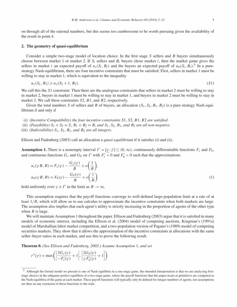
2. The geometry of quasi-equilibrium

Consider a simple two-stage model of location choice. In the first stage S sellers and B buyers simultaneouslychoose between market 1 or market 2. If Si sellers and Bi buyers chose market i, then the market game gives thesellers in market i an expected payoff of us(Si,Bi) and the buyers an expected payoff of ub(Si,Bi).5 In a pure-strategy Nash equilibrium, there are four incentive constraints that must be satisfied: First, sellers in market 1 must bewilling to stay in market 1, which is equivalent to the inequality

us(S1,B1) � us(S2 + 1,B2). (S1)

We call this the S1 constraint. Then there are the analogous constraints that sellers in market 2 must be willing to stayin market 2, buyers in market 1 must be willing to stay in market 1, and buyers in market 2 must be willing to stay inmarket 2. We call these constraints S2,B1, and B2, respectively.

Given the total numbers S of sellers and B of buyers, an allocation (S1, S2,B1,B2) is a pure-strategy Nash equi-librium if and only if

(i) (Incentive Compatibility) the four incentive constraints S1, S2,B1,B2 are satisfied.(ii) (Feasibility) S1 + S2 = S, B1 + B2 = B , and S1, S2, B1, and B2 are all non-negative.

(iii) (Indivisibility) S1, S2, B1, and B2 are all integers.

Ellison and Fudenberg (2003) call an allocation a quasi-equilibrium if it satisfies (i) and (ii).

Assumption 1. There is a nonempty interval Γ = [γ , γ̄ ] ⊂ (0,∞), continuously differentiable functions Fs and Fb ,and continuous functions Gs and Gb on Γ with F ′

s < 0 and F ′b > 0 such that the approximations

us(γB,B) = Fs(γ ) − Gs(γ )

B+ o

(1

B

),

ub(γB,B) = Fb(γ ) − Gb(γ )

B+ o

(1

B

)(1)

hold uniformly over γ ∈ Γ in the limit as B → ∞.

This assumption requires that the payoff functions converge to well-defined large-population limit at a rate of atleast 1/B , which will allow us to use calculus to approximate the incentive constraints when both markets are large.The assumption also implies that each agent’s utility is strictly increasing in the proportion of agents of the other typewhen B is large.

We will maintain Assumption 1 throughout the paper. Ellison and Fudenberg (2003) argue that it is satisfied in manymodels of economic interest, including the Ellison et al. (2004) model of competing auctions, Krugman’s (1991a)model of Marshallian labor market competition, and a two-population version of Pagano’s (1989) model of competingsecurities markets. They show that it allows the approximation of the incentive constraints at allocations with the sameseller–buyer ratios in each market, and use this to prove the following result.

Theorem 0. (See Ellison and Fudenberg, 2003.) Assume Assumption 1, and set

r∗(γ ) = max

(∣∣∣∣ 2Gs(γ )

−F ′s(γ )

+ 1

∣∣∣∣,∣∣∣∣2Gb(γ )

γF ′b(γ )

+ 1

∣∣∣∣)

5 Although the formal model we present is one of Nash equilibria in a one-stage game, the intended interpretation is that we are analyzing first-stage choices in the subgame-perfect equilibria of a two-stage game, where the payoff functions that this paper treats as primitives are computed asthe Nash equilibria of the game at each market. These payoff functions will typically only be defined for integer numbers of agents; our assumptionsare then on any extension of these functions to the reals.


and

α∗(γ ) = max{0,1/2 − 1/2r∗(γ )

}.

Then for any ε > 0, there exists a B such that for any integer B > B and any integer S with γ ≡ S/B ∈ Γ , the modelwith B buyers and S sellers has a quasi-equilibrium with B1 = α1B buyers in market 1, for every α1 ∈ [α∗(γ ) + ε,

1 − α∗(γ ) − ε].

The main focus of the paper will be on the exact equilibria, but as a preliminary step we provide a sharper charac-terization of the set of quasi-equilibria. The necessary condition we develop here may be of interest in its own right,and it will also be useful in our subsequent results.

Theorem 1. Assume Assumption 1. Define Γ ε = [γ + ε, γ̄ − ε], and set

T (γ ) = Gs(γ )

F ′s(γ )

− Gb(γ )

F ′b(γ )

,

and

α∗∗(γ ) = max

{0,

1

2− γ + 1

2|1 + γ − 2T (γ )|}.

Then for all ε > 0 there exists B such that for any integer B > B and any integer S with γ ≡ S/B ∈ Γ ε:

1. The model with B buyers and S sellers has a quasi-equilibrium with α1B buyers in market 1, for every α1 ∈[α∗∗(γ ) + ε,1 − α∗∗(γ ) − ε].

2. The model with B buyers and S sellers has no quasi-equilibria with B1 = α1B buyers and S1 sellers in market 1,B2 buyers and S2 sellers in market 2, provided B1/S1,B2/S2 ∈ Γ ε and α1 ∈ [ε,α∗∗(γ ) − ε] ∪ [1 − α∗(γ ) + ε,

1 − ε].

Remark. The difference between Theorems 0 and 1 is that the proof of Theorem 0 constructed quasi-equilibria withexactly equal seller–buyer ratios in each market, while Theorem 1 works with the full set of allocations. Since theproof of the theorem uses the approximation of the utility functions provided by Assumption 1, it is interesting to notethat it gives exactly the range of solutions that Ellison et al. (2004) obtained for the exact utility functions that arisewith uniformly distributed buyer values in their auction model. Note that the necessity result in 2. requires two extraconditions. The proposition only applies to equilibria with B1/S1,B2/S2 ∈ Γ ε because Assumption 1 imposes norestrictions at all on payoffs for γ /∈ Γ .6 We restrict attention to α1 /∈ {0,1} because the models often have equilibriawith all activity in a single market. The further restriction to α1 ∈ [ε,1 − ε] ensures that B1 and B2 are both large,which is necessary because Assumption 1 only characterizes payoffs in the large B limit.

The proof of Theorem 1 uses a lemma which notes that the S1, S2, B1, and B2 constraints can be rewritten in afairly simple form when the number of buyers is large.

Lemma 1. For all ε > 0, there is a B such that if B < B1,B2 and γ ≡ S/B ∈ Γ ε , then for α1 ≡ B1/B we have

1. If

(S1 − γB1) − Gs(γ )(1 − 2α1)

F ′s(γ )

∈ (α1 − 1 + ε,α1 − ε) (2)

and

(S1 − γB1) − Gb(γ )(1 − 2α1)

F ′b(γ )

∈ (−α1γ + ε, (1 − α1)γ − ε)

(3)

6 Alternatively, we could have allowed Γ = (0,∞) and weakened Assumption 1 to require that uniformity hold over compact subsets of Γ ,rather than all of Γ . Then Theorem 3 remains true, and Theorem 1 remains true provided we define Γε = [ε,1/ε]. Theorem 2, however, does notgeneralize in this way.


then there is a quasi-equilibrium with B1 buyers and S1 sellers in market 1.2. If S1/B1 ∈ Γ ε , S2/B2 ∈ Γ ε , and

(S1 − γB1) − Gs(γ )(1 − 2α1)

F ′s(γ )

/∈ [α1 − 1 − ε,α1 + ε],or

(S1 − γB1) − Gb(◦γ )(1 − 2α1)

F ′b(γ )

/∈ [−α1γ − ε, (1 − α1)γ + ε],

then there is no quasi-equilibrium with B1 buyers and S1 sellers in market 1.

The proof of Lemma 1 is presented in Appendix A.

Proof of Theorem 1. Lemma 1 implies that if B is large and S/B ∈ Γ ε , then the model with S sellers and B buyershas a quasi-equilibrium with B1 = α1B buyers in market 1 for all α1 for which there is a solution to the equations

(S1 − γB1) − Gs(γ )(1 − 2α1)

F ′s(γ )

∈ (α1 − 1 + ε,α1 − ε), and

(S1 − γB1) − Gb(γ )(1 − 2α1)

F ′b(γ )

∈ (−α1γ + ε, (1 − α1)γ − ε).

We can find an S1 that satisfies both conditions if and only if the intervals (α1 −1+ (Gs(γ )(1−2α1)

F ′s (γ )

− Gb(γ )(1−2α1)

F ′b(γ )

) + ε,

α1 + (Gs(γ )(1−2α1)

F ′s (γ )

− Gb(γ )(1−2α1)

F ′b(γ )

) − ε) and (−α1γ + ε, (1 − α1)γ − ε) intersect.

Given our definition T (γ ) = Gs(γ )F ′

s (γ )− Gb(γ )

F ′b(γ )

, this is equivalent to(α1 − 1 + ε + T (γ )(1 − 2α1), α1 − ε + T (γ )(1 − 2α1)

) ∩ (−α1γ + ε, (1 − α1)γ − ε) �= ∅.

The two intervals in this equation are of length 1 − 2ε and γ − 2ε, respectively, and they are both centered at 0when α1 = 1

2 . The first interval moves linearly with slope 1 − 2T (γ ) in response to changes in α1, while the secondinterval moves linearly with slope −γ , so the movement of the first interval, relative to the second, is linear with slope1 + γ − 2T (γ ) in response to changes in α1. The two intervals continue to intersect as long as the magnitude of therelative movement is less than (1 + γ )/2 − 2ε, which is true whenever |α1 − 1

2 | < (1+γ )/2−2ε|1+γ−2T (γ )| , i.e. when

α1 ∈(

1

2− 1 + γ − 4ε

2|1 + γ − 2T (γ )| ,1

2+ 1 + γ − 4ε

2|1 + γ − 2T (γ )|)

. (4)

Going from this expression to the simpler statement given in part 1 of the theorem would be a simple relabelingof the ε, but for the fact that |1 + γ − 2T (γ )| term in the denominator is not bounded below. This can be dealt withwithout much more work by dividing the γ ’s into two cases.

Partition Γ ε = Γ ε1 ∪ Γ ε

2 , where

Γ ε1 =

{γ ∈ Γ ε:

1 + γ

2|1 + γ − 2T (γ )| >2

3

}.

For γ ∈ Γ ε1 note that for any ε < 1/16 we have 1+γ−4ε

1+γ> 3

4 . Hence

1 + γ − 4ε

2|1 + γ − 2T (γ )| >3

4

1 + γ

2|1 + γ − 2T (γ )| >3

4

2

3= 1

2,

which implies that the interval in (4) is (0,1). Hence, if we are given any ε > 0, we can choose B to be equal to1/ε times the value B (call it B1/16) which makes the conclusion of Lemma 1 true for ε = 1/16. For B > B andα ∈ (ε,1 − ε) we have α1B > B1/16, (1 − α1)B > B1/16, and that α1 is in the interval identified in (4). Hence, thereis a quasi-equilibrium with B1 = α1B .

For γ ∈ Γ ε2 we have |1 + γ − 2T (γ )| > 2(1 + γ )/3 > 2/3, so we can just do a simple relabeling of ε: Given any

ε′ > 0, pick B such that the conclusion of Lemma 1 is true for ε = ε′/3 whenever B > (α∗∗(γ ) + ε′)B . Then for


B > B , we have quasi-equilibria for all α1 in the interval identified in (4), which contains (α∗∗(γ ) + ε′,1 − α∗∗(γ ) −ε′) when ε = ε′/3 and |1 + γ − 2T (γ )| > 2/3.

The proof of part 2. of the theorem uses part 2. of Lemma 1 in a nearly identical way. As long as B1 and B2 areboth large we know that there is no quasi-equilibrium with S1/B1, S2/B2 ∈ Γ ε if

α1 /∈(

1

2− 1 + γ + 4ε

2|1 + γ − 2T (γ )| ,1

2+ 1 + γ + 4ε

2|1 + γ − 2T (γ )|)

.

For γ ∈ Γ ε2 , the conclusion of part 2. of the theorem follows from a relabeling of the ε’s. For γ ∈ Γ ε

1 , the conclusionof part 2. is completely vacuous. �

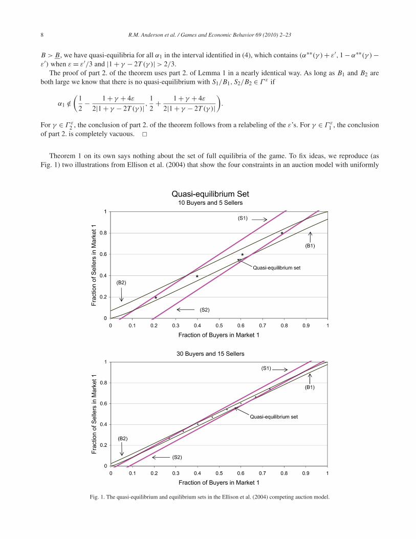
Theorem 1 on its own says nothing about the set of full equilibria of the game. To fix ideas, we reproduce (asFig. 1) two illustrations from Ellison et al. (2004) that show the four constraints in an auction model with uniformly

Fig. 1. The quasi-equilibrium and equilibrium sets in the Ellison et al. (2004) competing auction model.


distributed buyer values.7 Here the lines S1, S2, B1, B2 correspond to the points where the corresponding incentiveconstraints hold with equality. That is, along S1, each seller that is currently choosing market 1 is just indifferentbetween staying in market 1 or switching to market 2. Since sellers prefer there to be fewer other sellers, the pointsabove this line are not consistent with equilibrium. Reasoning in this way about each of the incentive constraints,we see that the quasi-equilibrium set is the diamond-shaped region in the center of the figure. The exact equilibria,marked with stars, are the integer grid points that lie in the quasi-equilibrium set.

The top panel corresponds to a model with ten buyers and five sellers. In equilibrium the smaller market can havetwo buyers and one seller, or four buyers and two sellers; there is no equilibrium with three or five buyers in the smallermarket. With three buyers in the smaller market, for example, there are a range of values of near one-and-a-half thatsatisfy the quasi-equilibrium conditions, but none of them satisfy the integer constraints. The bottom panel gives anidea of what happens as markets grows to thirty buyers and fifteen sellers. The quasi-equilibrium region looks much“flatter” because the impact of one agent moving from one market to another is smaller, so the utilities in the twomarkets need to be closer together in order to discourage agents whose equilibrium utility is lower from switchingmarkets. (Lemma 4 makes a related observation: If (S1, S2,B1,B2) is a quasi-equilibrium, then the seller–buyer ratioin market 1 must equal the overall ratio S/B plus a term that goes to 0 at rate O(1/B1).) The exact equilibria are againmarked with stars.

This leads us to the current question: when will there be exact equilibria? As the economy grows, the quasi-equilibrium set gets “narrower,” suggesting it might be harder to find an equilibrium at a given point, but at the sametime there are more candidate integers in a given range of relative sizes, so the answer may not be obvious.

3. An example with complete tipping

The main result of Ellison and Fudenberg (2003) is that models satisfying Assumption 1 always have a largeplateau of quasi-equilibria with two active markets when the number of agents is large. In this section, we show thatthe result does not always extend to a true equilibrium analysis. In particular, we provide a class of sequences ofeconomies in which the increasing returns satisfy Assumption 1, but which have no pure strategy equilibria other thanthe completely “tipped” equilibria with all activity in one market.

Example 1. Let us and ub be utility functions satisfying Assumption 1. Suppose that us(γB,B) is increasing in B

and decreasing in γ , and that ub(γB,B) is increasing in B and γ . Then, regardless of the size of B , a model with B

buyers and S = B + 1 sellers has no pure strategy Nash equilibrium with two active markets.

Proof. Suppose to the contrary that there is an equilibrium with 0 < B1 < B and 0 < S1 < S sellers in market 1, andB2 = B − B1 buyers and S2 = S − S1 sellers in market 2, and assume without loss of generality that B1 � B2.

We proceed to rule out all possible relationships between S1 and B1

• If S1 < B1, then a buyer in market 1 will defect. After the defection market 2 will be larger (have more buyers)and have a more favorable seller–buyer ratio for buyers.

• If S1 = B1, then a buyer in market 1 will defect. Market 2 is larger after the defection. Also, S1 = B1 impliesS2 = B2 + 1, so after the defection the ratio of sellers to buyers in market 2 becomes one, the same as in market1. Hence, the buyer is better off after the defection

• If S1 = B1 + 1 and B1 = B2, then a buyer in market 2 will defect. S2 = B2 so the situation is exactly as in the caseabove, but with the labels reversed.

• If S1 = B1 + 1 and B1 < B2, then a seller in market 1 will defect. Market 2 is larger, and even after the defectionits seller–buyer ratio is lower: (S2 + 1)/B2 = (B2 + 1)/B2 < (B1 + 1)/B1 = S1/B1.

• If S1 > B1 + 1, then a seller in market 1 will defect. Market 2 is at least as large, and even after the deviation itwill have a lower seller–buyer ratio. �

7 In Ellison et al. (2004), each seller has a single unit to sell, and reservation value 0 for keeping the item; each buyer wants to purchase a singleunit, and buyer values are determined after location choice. Equilibrium thus payoffs in each market are determined by a uniform-price auction.


In some sense the assumption that S = B + 1 in the example is a worst case for the existence of equilibria. Equi-librium requires that the seller–buyer ratios be very close in the two markets. When market 1 and market 2 are aboutthe same size, the fact that we have to put the one extra seller somewhere means we have to have about one-half toofew sellers in one market and about one-half too many sellers in the other. The “market impact” of moving to the largemarket is one seller or one buyer, so it doesn’t outweigh this. This suggests that finding equilibria may be easier whenthe seller–buyer is bounded away from 1, as then the impact of the “rounding error” is less severe. More generally,one way of looking at the example is that the size of the set of equilibria will depend on how closely the overallseller–buyer ratio can be approximated in the two markets when we are restricted to integer allocations.

4. A sufficient condition for a plateau of equilibria in large finite economies

In this section we provide sufficient conditions for the existence of a plateau of true equilibria. The sufficientconditions illustrate that the nonexistence example was special. In the example, the seller–buyer ratio is very closeto one, but not equal to one. The main proposition of this section shows that if the ratio of the number of agentson the two sides of the market is not almost exactly an integer (and the number of agents is large), then there is anondegenerate plateau of untipped equilibria. It also shows that within the equilibrium plateau the equilibria are nottoo far apart.

Let N be the set of non-negative integers. The main result of this section is

Theorem 2. Fix functions ub and us satisfying Assumption 1. There are constants α, k1, k2, k3, k4 with α < 1/2 suchthat for any ε > 0, any α ∈ [α,1 − α], and any positive integers B and S satisfying

(i) S/B ∈ Γ ,(ii) |B/S − n| > ε and |S/B − n| > ε for all n ∈ N, and

(iii) B + S > k1 + k2/ε,

the model with B buyers and S sellers has an equilibrium with B1 buyers and S1 sellers in market 1 for some B1, S1with |B1/B − α| < (k3 + k4/ε)/B and |S1/S − α| < (k3 + k4/ε)/S.

The proof includes more information on the constants k1, k2, k3, and k4, including explicit formulas for some ofthem. The following corollary is a simpler statement about the existence of an equilibrium plateau.

Corollary 1. Fix functions ub and us satisfying Assumption 1. Then there is α < 1/2 such that for any ε > 0 and anyδ > 0 there is an M such that if

(i) S/B ∈ Γ ,(ii) |B/S − n| > ε and |S/B − n| > ε for all n ∈ N, and

(iii) B + S > M ,

then for every α ∈ [α,1 − α], the model with B buyers and S sellers has an equilibrium with B1 buyers and S1 sellersin market 1 for some B1, S1 with |B1/B − α| < δ and |S1/S − α| < δ.

The intuition for this result starts from the observation that not only are the quasi-equilibrium constraints satisfiedat the allocation (S/2, S/2,B/2,B/2), they are satisfied with enough slack that the S1 and S2 constraints are alsosatisfied at (S/2 − 1/2, S/2 + 1/2,B/2,B/2).8 Hence, when B is even, there is always an integer S1 for which theS1 and S2 constraints are both satisfied at (S1, S − S1,B/2,B/2).

To show that the S1 and S2 constraints can be satisfied for some integers S1,B1 near any given B ′1 that is close

to B/2 one can argue as follows. Using continuity (S1, S − S1,B1,B − B1) will satisfy the S1 and S2 constraintsif S1 ∈ [γB1 − (1/2 − ε/2), γB1 + (1/2 − ε/2)] and B1 is within some distance of B/2. Suppose B ′

1 is within this

8 At this allocation a seller who moves to market 1 will make it identical to market 2, so it is no longer better for sellers.


distance of B/2. Because ε > 0, there may be no S1 for which (S1, S − S1,B′1,B − B ′

1) satisfies the S1 and S2constraints. However, this can only happen if γB ′

1 is within ε/2 of being one half more than an integer. If this istrue, consider a split with B ′′

1 = B ′1 − 1 buyers in market 1. There must be an integer split satisfying the S1 and S2

constraints with B1 = B ′′1 unless γB ′′

1 = γ (B ′1 − 1) = γB ′

1 − γ is also within ε/2 of being one-half more than aninteger. It is impossible for γB ′

1 and γB ′1 − γ to both be this close to one-half more than an integer unless γ itself is

within ε of being an integer. Hence, we know there is an integer allocation for B1 very close to B ′1 that satisfies the

S1 and S2 constraints.The argument above only deals with the S1 and S2 constraints. The full proof is a bit more complicated because it

also deals with the B1 and B2 constraints (which are only satisfied for a narrower range of S1).

Proof of Theorem 2. We proceed in two main steps. The first step is to show that the quasi-equilibrium set contains aparallelogram in B-S space that includes all points on the line segment defined by B1/B = S1/S and B1/B ∈ [α,1−α]and that is not “too thin.” The second step is to show that every point in the parallelogram is within a specified distanceof an integer point that is also within the parallelogram. The integer points are true equilibria.

To simplify the exposition we will prove the result only for pairs with S � B . “Sellers” and “buyers” are completelysymmetric in the model, so the argument for B � S would be identical.

Lemma 2. There exist α and N with α < 1/2 such that for all B and S with B + S > N and γ ≡ S/B ∈ Γ , it is aquasi-equilibrium of the model with B buyers and S sellers to have B1 buyers and S1 sellers in market 1 for any B1and S1 with and any B1, S1 with B1/B ∈ [α,1 − α] and |S1/S − B1/B| � 1/4B .

Remark. When we graph the space of allocations as in Figs. 1 and 2, with B1/B on the x-axis and S1/S, on the y-axis, the lemma says that the quasi-equilibrium set contains the parallelogram bounded by (α,α ± 1/4B) and (1 − α,

1 − α ± 1/4B).

Proof of Lemma 2. We will show that buyers in market 1 do not wish to switch to market 2, i.e. that the B1 constraintis satisfied. The argument for the B2 constraint is identical. The arguments for the S1 and S2 constraints are verysimilar.

We begin with the “hardest” case for the B1 constraint: when S1 = (α − 1/4B)S and B1 = αB . In this case weneed to show that

ub

((α − 1/4B)S,αB

)� ub

((1 − α + 1/4)S, (1 − α)B + 1

).

Given Assumption 1, this will be satisfied whenever B + S is greater than some N if

Fb

(γ

(1 − 1

4αB

))− Gb

(γ

(1 − 1

4αB

))1

αB

> Fb

(γ

(1 − 3

4(1 − α)B

))− Gb

(γ

(1 − 3

4(1 − α)B

))1

(1 − α)B

whenever B is greater than some B . (The restriction to S/B ∈ [γ , γ ] ⊂ (0,∞) implies that B is always large whenB + S is large.) There exists B so that this is true for all B > B if for all γ ∈ Γ and all α ∈ [α,α] we have(

− 1

4α+ 3

4(1 − α)

)γF ′

b(γ ) >

(1

α− 1

1 − α

)Gb(γ ),

which is equivalent to

α − 1/4

1 − 2α>

Gb(γ )

γF ′b(γ )

.

We can choose α ∈ (1/4,1/2) so that this is true uniformly over γ . Note that for the same α the equation we wouldhave derived had we started with any larger S1 will also be satisfied due to the monotonicity of Fb . Hence, havingchosen an α satisfying this equation we can then choose B so that B1 is satisfied for all B1 and S1 in the parallelogramprovided that B > B , which completes the proof of Lemma 2. �


Given the result of Lemma 2 it suffices to prove the following lemma about parallelograms containing grid points.Lemma 3 concludes that there exist integers B1 and S1 satisfying several properties. The first two of these are that(B1/B,S1/S) belongs to the parallelogram described in Lemma 2, which implies that it is a true equilibrium to haveB1 buyers and S1 sellers in market 1. The last two indicate we can find such equilibria close to every point of theplateau identified in the theorem.

Lemma 3. Assume α < 1/2. Then there are constants k1, k2, k3, k4 such that for any ε > 0, any α ∈ [α,1 − α] andany S,B satisfying

(i) S � B ,(ii) S/B ∈ Γ ,

(iii) |B/S − n| > ε for all n ∈ N , and(iv) S > k1 + k2/ε,

there exist integers S1 and B1 such that B1/B ∈ [α,1 −α], |S1/S −B1/B| < 1/4B , |B1/B −α| < (k3 + k4/ε)(1/B),and |S1/S − α| < (k3 + k4/ε)(1/S).

Proof of Lemma 3. Fix some α ∈ [α,1 − α]. We assume here that α > 1/2. (A symmetric argument applies forα < 1

2 .)Let B0

1 be the integer closest to αB in the set of integers B ′ such that B ′/B ∈ (α,1− α). (This set will be non-emptyfor k1 sufficiently large given the assumption that S/B ∈ Γ .)

We now define a sequence of integer pairs (Sk1 ,Bk

1 ) by repeatedly reducing S1 by one and B1 by an integer closeto B/S. We will choose (S1,B1) to be the first point in the sequence that satisfies |Sk

1/S − Bk1/B| < 1/4B . The key

observation is that this always occurs for some k with k � 4 + 1/ε.Let S1

1 = �(B01/B)S�. Note that S1

1/S � B01/B . Let B1

1 be the largest integer with B11/B � S1

1/S + 1/4B .If S1

1/S < B11/B + 1/4B , then choose we will choose S1 = S1

1 and B1 = B11 . Note in this case that S1 and B1

satisfy |S1/S − B1/B| < 1/4B .Otherwise, if for some k � 1 we have Sk

1/S � Bk1/B + 1/4B , then define Sk+1

1 and Bk+11 by Sk+1

1 = Sk1 − 1, and

Bk+11 =

{Bk

1 − �B/S� if B/S − �B/S� � Sk1/S − Bk

1/B + 1/4B

Bk1 − �B/S� − 1 if B/S − �B/S� > Sk

1/S − Bk1/B + 1/4B

.

We then choose (S1,B1) = (Sk1 ,Bk

1 ) where k is the smallest index for which |Sk1/S − Bk

1/B| � 1/4B .Claim: This choice of (S1,B1) is well-defined and the index k satisfies k � 3 + 1/ε.

To show this, we write x for B/S − �B/S� and define ak ≡ B(Sk1/S − Bk

1/B − 1/4B). Note that (Sk1 ,Bk

1 ) are thedesired (S1,B1) if ak ∈ (−1/2,0].

The definition of B11 as the largest integer satisfying B1

1/B � S11/S + 1/4B implies that (B1

1 + 1)/B > S11/S +

1/4B , a1 = B(S11/S − B1

1/B − 1/4B) ∈ [−1/2,1/2).If (S1

1 ,B11 ) is not the desired pair of integers, then a1 ∈ (0,1/2). For ak ∈ (0,1/2) the expressions for Sk+1

1 ,Bk+11

can be rewritten as

Sk+11 = Sk

1 − 1,

Bk+11 =

{Bk

1 − �B/S� if x � ak + 1/2Bk

1 − �B/S� − 1 if x > ak + 1/2.

Hence,

ak+1 ={

B(Sk+1

1S

− Bk+11B

− 14B

) = B(Sk

1S

− 1S

− Bk1

B− �B/S� − 1

4B

) = ak − x if x � ak + 1/2ak + (1 − x) if x > ak + 1/2

.

We complete the proof of our claim by considering two cases:


Case 1: x � 1/2.In this case the dynamics are ak+1 = ak −x whenever ak > 0. Hence we have ak ∈ [−1/2,0) for k = 1+� a1−x

x� <

2 + 1/x � 1 + 2/ε.Case 2: x > 1/2.

If a1 ∈ [−1/2,0], then (S11 ,B1

1 ) has the desired property. If a1 ∈ [x − 1/2,1/2), then a2 = a1 − x ∈ [−1/2,0], so(S2

1 ,B21 ) has the desired property. Finally, if a1 ∈ (0, x − 1/2), then a2 = a1 + 1 − x, and aj+1 = aj + 1 − x for all

j with aj ∈ (0, x − 1/2). Hence, a1+�(x−1/2−a1)/(1−x)� ∈ (x − 1/2,1/2). Hence (Sk,Bk) has the desired property fork = 2 + �(x − 1/2 − a1)/(1 − x)� � 2 + �1/2(1 − x)� � 3 + 1/2ε.

The statement of the Lemma requires that (S1,B1) have four properties (which hold uniformly given some choiceof k1, k2, k3, and k4).

The first of these was that B1/B ∈ [α,1 − α]. It is immediate from out construction that B1 ∈ [B01 − k�B/S�,

B01 for k � 3 + 1/ε. The fact that B0

1/B � 1 − α implies B1/B � 1 − α. Given that α � 1/2 we have B1/B �1/2 − 1/B − (3 + 1/ε)(1/S + 1/B). This is greater than α when B > k1 + k2/ε given an appropriate choice of k1and k2.

The second of these was that |S1/S − B1/B| < 1/4B . We chose (S1,B1) so that this holds.The third is that |B1/B − αB| < (k3 + k4/ε)(1/B). That we can choose k3 and k4 so that this is true again follows

easily from B1 ∈ [B01 − k�B/S�,B0

1 for k � 3 + 1/ε. The upper bound gives B1/B � B01/B � �αB/B� < α + (1/B).

The lower bound gives B1/B < α − 1/B − (3 + 1/ε)(�B/S�). Using �B/S� < 2(B/S), this is greater than α − (k3 +k4/ε)(1/B) for k3 = 7 and k4 = 2.

The argument for the fourth condition is similar, but simpler because Sk1 = S1

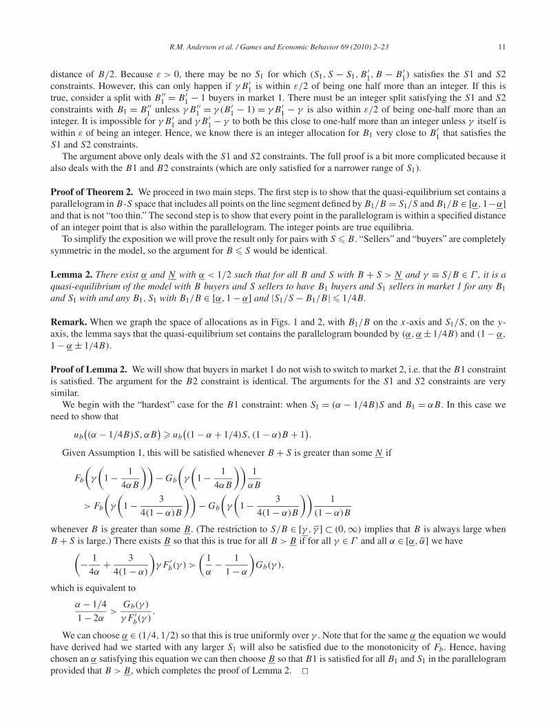
1 − (k − 1).This finishes the proof of Lemma 3, and thus proves the theorem. �Fig. 2 provides some intuition for Lemma 3. It shows a magnified view of the parallelogram {(x, y): x ∈ [α,

1 − α], |y − x| < 1/4B} passing through the lattice {(x, y): ∃B1, S1 with x = B1/B,y = S1/S}. The parallelogramis half as wide as the gap between adjacent x’s, so for a given value of y the parallelogram need not intersect anygrid points, e.g. in the top row of the grid the parallelogram passes between (B1

1/B,S11/S) and ((B1

1 + 1)/B,S11/S).

Because B/S is not an integer, the parallelogram is shifted relative to the grid at different y values. The figure hasB/S = 1.3, so the intersection shifts to the left by 1.3 grid points when y is reduced to (S1

1 − 1)/S. This impliesthat the parallelogram will intersect the grid at least once in every three adjacent rows. When B/S is ε away from aninteger, the number of consecutive rows that can have no intersection is larger, but still bounded above by 1 + 1/2ε.

Our theorem shows that we get a plateau of true equilibria whenever the seller–buyer ratio (and the buyer–sellerratio) is not too close to an integer. The example of the previous section was one where Sn/Bn was becoming closerand closer to one as n increased. It is closeness to an integer, not being exactly equal to an integer, that can lead tononexistence. If the buyer–seller ratio is exactly equal to an integer, then an analogue to Theorem 2 would hold, and

Fig. 2. Illustration of Lemma 3.


in fact we would obtain an even stronger result: there would be an exact equilibrium for every S1 in the specifiedrange.9 We should also note that having the buyer–seller ratio close to an integer does not always lead to nonexistenceof split-market equilibria. For example, there will be a plateau of equilibria even when Sn/Bn → 1 provided thatSn + Bn is even for all n, since that permits us to find an integer pair in the parallelogram of quasi-equilibria.

5. The density of the set of equilibria

In this section we provide a characterization of the equilibrium set for large finite economies. Roughly, we showthat in most large economies the equilibrium set fills out a wide plateau and we specify the density of equilibria withinthe plateau. Moreover, there exists an α∗∗ < 1

2 depending on γ such that the density is as large as possible whenthe fraction of agents in the smaller market is at least α∗∗. If there are fewer sellers than buyers, then essentially allintegers S1 in (Sα∗∗, S(1 − α∗∗)) there is an equilibrium with S1 sellers in market 1. If there are fewer buyers thansellers, then for essentially all integers B1 in (Bα∗∗(γ ),B(1 − α∗∗(γ )), there is an equilibrium with B1 sellers inmarket 1. More precisely, our theorem provides two results of this type. The first shows that given any sequence ofeconomies {Bn,Sn} with Sn/Bn converging to an irrational limit, the width of the equilibrium plateau and the densityof equilibria within it converge to the functions we identify as n → ∞. The second shows that if a large economy isselected at random by choosing the buyer–seller ratio to approximate a random draw from a nonatomic distributionthen the probability that the equilibrium set will be within any ε of the limiting characterization converges to one asthe number of buyers increases.

Although the proof uses nonstandard analysis, the statement of Theorem 3 is completely standard and can beunderstood without any knowledge of nonstandard analysis. The statements of the lemmas do involve nonstandardanalysis. Before each of the nonstandard statements, we give the intuition behind the statement, to assist readersunfamiliar with nonstandard analysis. Similarly, before each of the proofs, we give an outline of the intuition behindthe nonstandard proof.

In the following definition, N (B,S) is essentially the set of B1 such that in the model with B buyers and S sellers,there is an equilibrium with B1 buyers in market 1.10

Definition 1. Let N (B,S) denote the set of all B1 ∈ {0,1, . . . ,B} such that there exists S1 ∈ {0,1, . . . , S} such that

1. the market with B buyers and S sellers has a Nash equilibrium with B1 buyers and S1 sellers in market 1; and2. if we define S2 = S − S1 and B2 = B − B1, then{

S1

B1,S2

B2,S1 + 1

B1,S2 + 1

B2,

S1

B1 + 1,

S2

B2 + 1

}⊂ Γ.

The following definition specifies, for each γ , a piecewise linear function of α which is strictly positive on an openinterval containing α = 1

2 . We shall see that the density of the set N (B,S) converges to this piecewise linear function.

Definition 2. Let

T (γ ) = Gs(γ )

F ′s(γ )

− Gb(γ )

F ′b(γ )

,

α∗(γ ) = max

{0,

1

2− γ + 1

2|1 + γ − 2T (γ )|},

α∗∗(γ ) = max

{0,

1

2− |γ − 1|

2|1 + γ − 2T (γ )|},

9 This is true if S � B . When B � S there would be an exact equilibrium for every B1 in the range.10 N (B,S) is actually a slightly smaller set than the one just described, because of condition 2. If S1

B1/∈ Γ , or S2

B2/∈ Γ , or a defection by one

player could take the ratio of the sellers to buyers in that player’s new market outside of Γ , then Assumption 1 gives us no control over payoffs,and hence makes it impossible to prove that a given pair (B1, S1) is not an equilibrium. Because the set we identify is no larger than the set ofequilibria, the density of the set of all equilibria, including equilibria with ratios outside Γ , will be at least as great as indicated in Theorem 3.


H(α,γ ) =

⎧⎪⎪⎪⎪⎪⎨⎪⎪⎪⎪⎪⎩

0 if α ∈ [0, α∗(γ )](α−α∗(γ ))min{1,γ }

α∗∗(γ )−α∗(γ )if α ∈ (α∗(γ ),α∗∗(γ ))

min{1, γ } if α ∈ [α∗∗(γ ), 1 − α∗∗(γ )](1−α−α∗(γ ))min{1,γ }

α∗∗(γ )−α∗(γ )if α ∈ (1 − α∗∗(γ ),1 − α∗(γ ))

0 if α ∈ [1 − α∗∗(γ ),1]

. (5)

Our theorem characterizes the local density of equilibrium throughout the equilibrium plateau. To simplify thestatement of the theorem we first define this object.

Definition 3. Given an economy {B,S} and ε > 0 with Bε > 1, the ε-local density of equilibria at α in the economyis

Hε(B,S,α) ≡ Prob{B1 ∈ N (B,S): B1 ∈ N, |B1/B − α| < ε

},

where the probability is with respect to a uniform distribution over all integers B1 satisfying the constraint|B1/B − α| < ε.

Theorem 3. Suppose Assumption 1 holds, Bn ∈ N, Bn → ∞, εn > 0, εn → 0, and εnBn → ∞.

1. If Sn is a sequence of positive integers with Sn

Bn→ γ ∈ (γ , γ̄ ) \ Q, then

supα∈[0,1]

∣∣Hεn(Bn,Sn,α) − H(α,γ )∣∣ → 0 as n → ∞.

2. Suppose that γn is a sequence of independent identically distributed random variables whose common distributionis absolutely continuous with respect to Lebesgue measure and has support contained in Γ and Sn = �γnBn�.Then,

supα∈[0,1]

∣∣Hεn(Bn,Sn,α) − H(α,γn)∣∣ → 0 in probability as n → ∞

i.e. for every δ > 0, there exists N ∈ N such that for every n > N ,

P(

supα∈[0,1]

∣∣Hεn(Bn,Sn,α) − H(α,γn)∣∣ > δ

)< δ.

Fig. 3 contains a graph of the function H(α,γ ) for the application considered in Fig. 1: the Ellison et al. (2004)competing auction model with S/B = 1

2 . In this case, we find α∗(γ ) = 1/8, α∗∗(γ ) = 3/8, and Min(1, γ ) = 1/2.Hence, when the number of buyers and sellers is large the equilibrium set includes splits with B1/B ranging from

Fig. 3. The density-of-equilibria function H(α,γ ).


about 1/8 to 7/8. The equilibrium set reaches a maximum density of 1/2 for values of α between 3/8 and 5/8. Thismeans that there are true equilibria for about half of the B1 in this range. There are only half as many sellers as buyers,so this means that there is an equilibrium for almost all S1 between 3

8S and 58S.

Before proving the theorem we first need some notation and two lemmas. We will suppose throughout thatB1,B2, S1, S2 ∈ N, B1 + B2 = B , S1 + S2 = S, γ1 = S1/B1, γ2 = S2/B2, α1 = B1/B . The proofs of the lemmasand theorem make use of nonstandard analysis. Let *N be the set of nonstandard integers, so that every n ∈ *N \ N isan infinite nonstandard natural number. Given any finite nonstandard number α, let ◦α denote the standard part of α,the unique standard real number infinitely close to α. We write x � y to mean that x − y is infinitesimal.

Our first lemma, Lemma 4, puts an upper bound on the equilibrium set: roughly it says that all equilibria must haveS1/B1 ≈ S/B if B is large. More formally, it is equivalent to the following standard statement: Suppose we considera sequence of models with Sn sellers and Bn buyers, with Sn → ∞ and Bn → ∞. Suppose Sn1,Bn1 ∈ N, Sn1 � Sn,Bn1 � Bn. Suppose there exists ε > 0 such that Sn/Bn ∈ [γ + ε, γ̄ − ε] and Bn1/Bn ∈ [ε,1 − ε] for all n. Write γn

for Sn/Bn and γn1 for Sn1/Bn1. Then, if Bn|γn1 − γn| → ∞, there exists N such that for all n > N , the model withSn sellers and Bn buyers has no equilibrium with Bn1 buyers and Sn1 sellers in market 1.

For the proof, consider a seller located in the market with a higher ratio of sellers to buyers, which we may assumewithout loss of generality to be market 1. Since F ′

s(γ ) < 0 for all γ ∈ Γ and Γ is compact, F ′s(γ ) is uniformly

bounded away from zero. By the Mean Value Theorem, the benefit to the seller in switching to market 2 containsa term which is bounded below by (minγ∈Γ |F ′

s(γ )|)(γn2 − γn1) > 0; this term dominates the other terms becauseBn|γn1 − γn| → ∞, and it follows that the seller would benefit from switching markets.

Lemma 4. Suppose S,B ∈ *N \ N, ◦γ ∈ (γ , γ̄ ), and ◦α1 ∈ (0,1), Then if γ1 �= γ + O( 1B1

), there is no equilibriumwith B1 buyers and S1 sellers in market 1.

Proof of Lemma 4. We may assume without loss of generality that γ1 > γ2. Consider a seller contemplating switch-ing from market 1 to market 2. The change in the seller’s payoff resulting from the switch is

Fs

(γ2 + 1

B2

)− Gs(γ2 + 1

B2)

B2− Fs(γ1) + Gs(γ1)

B1+ o

(1

B1

)

� max{F ′

s(γ′): γ ′ ∈ Γ

}(γ2 − γ1 + 1

B2

)+ O

(1

B1

)> 0

provided ◦γ1 ∈ (γ , γ̄ ) and ◦γ2 ∈ (γ , γ̄ ), which shows there is no equilibrium with B1 buyers and S1 sellers in mar-ket 1. �

The previous lemma formalizes the observation that the “diamond” of quasi-equilibria becomes flatter as the econ-omy grows so that splits of agents between the markets with γn1 �≈ γn will not give equilibria. The next step is tocharacterize which splits with γn1 ≈ γn are indeed compatible with the incentive constraints. Ellison and Fudenberg(2003) gave a sufficient condition for incentive compatibility that assumed γ1 = γ2 = γ . The next lemma improves onit by considering all γ1 that are consistent with the previous lemma.

The following nonstandard lemma is equivalent to the following, rather complicated, standard statement: Supposewe consider a sequence of models with Sn sellers and Bn buyers, with Sn → ∞ and Bn → ∞. Suppose Sn1,Bn1 ∈ N,Sn1 � Sn, Bn1 � Bn. Write γn for Sn/Bn, γni for Sni/Bn1, and α̂ni for Bni/Bn. Suppose there exists ε > 0 such thatγn ∈ [γ + ε, γ̄ − ε] and α̂n1 ∈ [ε,1 − ε] for all n. Part 1 says that if the sequence {Bn|γn1 − γn|} is uniformly boundedand δ > 0, then for every subsequence nm such that Snm/Bnm converges to a limit γ , there exists N such that whenever

(Snm1 − γBnm1) − Gs(γ )(1 − 2α̂nm1)

F ′s(γ )

∈ (α̂nm1 − 1 + δ, α̂nm1 − δ)

and

(Snm1 − γBnm1) − Gb(γ )(1 − 2α̂nm1)

F ′b(γ )

∈ (−(α̂nm1)γ + δ, (1 − α̂nm1)γ − δ)


and nm > N , then there is an equilibrium with Bnm1 buyers and Snm1 sellers in market 1. Part 2 says suppose thatfor all n, γn1 ∈ [γ + ε, γ̄ − ε] and γn2 ∈ [γ + ε, γ̄ − ε]. Then for every δ > 0 and every subsequence nm such thatSnm/Bnm converges to a limit γ , there exists N such that whenever

(Snm1 − γBnm1) − Gs(γ )(1 − 2α̂nm1)

F ′s(γ )

/∈ (α̂nm1 − 1 − δ, α̂nm1 + δ)

or

(Snm1 − γBnm1) − Gb(γ )(1 − 2α̂nm1)

F ′b(γ )

/∈ (−(α̂nm1)γ − δ, (1 − α̂nm1)γ + δ)

and nm > N , then there is no equilibrium with Bnm1 buyers and Snm1 sellers in market 1. The nonstandard proof ofLemma 5 is a straightforward application of Lemma 1. The complication in the standard statement comes from thefact that N depends on both δ and the subsequence nm, and a standard proof would have to use the convergence ofγn = Sn/Bn to γ to change γn to γ in the statement.

Lemma 5. Suppose S,B ∈ *N \ N, ◦γ ∈ (γ , γ̄ ), and ◦α1 ∈ (0,1). Then

1. If γ1 = γ + O( 1B1

),

◦(S1 − γB1) − Gs(◦γ )(1 − 2◦α1)

F ′s(

◦γ )∈ (◦α1 − 1, ◦α1

)(6)

and

◦(S1 − γB1) − Gb(◦γ )(1 − 2◦α1)

F ′b(

◦γ )∈ (−◦α1

◦γ,(1 − ◦α1

)◦γ)

(7)

then there is an equilibrium with B1 buyers and S1 sellers in market 1.2. Suppose

◦(

S1

B1

)∈ (γ , γ̄ ) and ◦

(S2

B2

)∈ (γ , γ̄ ).

If

◦(S1 − γB1) − Gs(◦γ )(1 − 2◦α1)

F ′s(

◦γ )/∈ [◦α1 − 1, ◦α1

]or

◦(S1 − γB1) − Gb(◦γ )(1 − 2◦α1)

F ′b(

◦γ )/∈ [−◦α1

◦γ,(1 − ◦α1

)◦γ]

then there is no equilibrium with B1 buyers and S1 sellers in market 1.

Proof of Lemma 5. For part 1, we may find ε ∈ R, ε > 0 such that

◦γ ∈ (γ + ε, γ̄ − ε),

◦(S1 − γB1) − Gs(◦γ )(1 − 2◦α1)

F ′s(

◦γ )∈ (◦α1 − 1 + ε, ◦α1 − ε

),

◦(S1 − γB1) − Gb(◦γ )(1 − 2◦α1)

F ′b(

◦γ )∈ (−◦α1

◦γ + ε,(1 − ◦α1

)◦γ − ε).

Find B ∈ N satisfying the conclusion of Lemma 1. Since Gs,F′s ,Gb,F

′b are continuous,

γ ∈ *(γ + ε, γ̄ − ε) = *Γε,

(S1 − γB1) − Gs(γ )(1 − 2α1)

F ′s(γ )

∈ *(α1 − 1 + ε,α1 − ε),

(S1 − γB1) − Gb(γ )(1 − 2α1)

F ′b(γ )

∈ *(−α1γ + ε, (1 − α1)γ − ε

).


Since ◦α1 ∈ (0,1), B1,B2 ∈ *N\N, so B1,B2 > B . Thus, we have verified the transfer of the hypotheses of Lemma 1.By the Transfer Principle, the transfer of Lemma 1 holds, so the conclusion of the transfer of Lemma 1 holds, butthis just says there is a quasi-equilibrium with B1 buyers and S1 sellers in market 1. Since B1,B2, S1, S2 ∈ *N, thisquasi-equilibrium is an equilibrium. The proof of part 2 is analogous. �Remark. The previous lemma characterizes the allocations of agents to each market that are consistent with theincentive constraints. Since the result uses the approximation of the utility functions provided by Assumption 1, it isinteresting to note that it gives exactly the range of solutions that Ellison et al. (2004) obtained for the exact utilityfunctions that arise with uniformly distributed buyer values in their auction model.

The statement of Theorem 3 is standard, but the proof is not; a standard proof would necessarily involve verycomplex ε, δ arguments. Here, we outline the main ideas. Lemma 4 shows that, in the limit, an equilibrium cannot existunless γn1 = Sn1/Bn1 is within O(1/Bn1) of γn = Sn/Bn. Lemma 5 shows that if γn1 = Sn1/Bn1 is within O(1/Bn1),then in the limit whether or not an equilibrium exists is determined by the relationship between Sn1 − γnBn1 andαn1 = Bn1/Bn. Recall that in characterizing the quasi-equilibrium set we defined

T (γ ) = Gs(γ )

F ′s(γ )

− Gb(γ )

F ′b(γ )

.

The two conditions for existence of an equilibrium in Lemma 5 together imply that for large n (Sn1, Sn2,Bn1,Bn2)

will be an equilibrium if Sn1 − γnBn1 lies in an interval very close to the interval[(αn1 − 1, αn1) + T (γn)(1 − 2αn1)

] ∩ (−αn1γn, (1 − αn1)γn

). (8)

A little algebra shows that the intersection of the two intervals on the RHS of Eq. (8) has length H(αn1, γn).There is an equilibrium for a given Bn1 if and only if there is an integer Sn1 for which Sn1 − γnBn1 falls into this

interval. The εn equilibrium density at α is the fraction of Bn1’s with |Bn1/Bn − α| < ε for which such an Sn1 exists.Let r : R → [0,1] denote the remainder function r(x) = x − �x�. Let Kn = �εnBn�, Kn = {−Kn,−Kn + 1,

. . . ,Kn}. Given k ∈ Kn, let Bnk = �αBn� + k and αnk = Bnk/Bn. These are the possible choices of Bn1 with Bn1/B

close to α. Since the interval [αnk − 1, αnk) has length 1, for each k there is exactly one integer Snk such that

Snk − γnBnk − Gs(γn)(1 − 2αnk)

F ′s(γn)

∈ [αnk − 1, αnk). (9)

Equilibrium will exist for a given k ∈ Kn if and only if, apart from a small δ, Eq. (8) is satisfied for Bnk and theunique Snk that satisfies Eq. (9). Some algebra reduces this to a condition on r(γnBnk). Since Bn(k+1) = Bnk + 1,r(γnBn(k+1)k) = r(γnBnk) + γn (modulo 1). By assumption in part 1, γn → γ for some irrational γ ∈ (γ , γ̄ ). Sinceγ is irrational, it is well known, and not difficult to show, that the proportion of k ∈ Kn such that r(γBnk) lies inany given interval converges to the length of that interval; see for example Exercise VII.8.9 in Dunford and Schwartz(1957).11 An ε, δ argument on the rate of convergence in the Ergodic Theorem and the rate at which irrational numberscan be approximated by rational numbers of a given denominator would allow one to show that the same conclusionholds if we replace γ with γn, which proves part 1.

The result in part 2 can be derived from the result in part 1 by a standard argument. To see this, let Yn(x) =supα |Hεn(Bn, �xBn�, α) − H(α,x)| for x ∈ Γ . The conclusion of part 1 says that limYn(x) = 0 whenever x isirrational, so Yn(x) → 0 almost everywhere, which implies that Yn(x) converges to zero in measure because Γ iscompact. Since the common distribution of the random variables γn is absolutely continuous with respect to Lebesguemeasure, supα |Hεn(Bn, �γnBn�, α) − H(α,γn)| converges to zero in probability.

Proof of Theorem 3. Consider three sequences Sn, Bn and εn satisfying the hypotheses of the theorem. Fix anyn ∈ *N \ N. Let S = Sn, B = Bn, γ̂ = Sn

Bn, ε = εn, K = �εnBn� and K = {−K,−K + 1, . . . ,−1,0,1, . . . ,K − 1,K}.

11 This is a very special case of the Ergodic Theorem. When γ is irrational, translation by γ , modulo 1, is an ergodic, measure-preservingtransformation from [0,1) to [0,1), i.e. if a measurable set V satisfies V + γ = V (modulo 1), then the measure of V is either zero or one, and forevery measurable set W ⊂ [0,1), W −γ (modulo 1) has the same measure as W . Note that if γ is rational, then γ = a/b where a and b are integerswith no common factor. Then translation by γ (modulo 1) is not ergodic because if W = [0,1/2b) ∪ [1/b,3/2b) ∪ · · · ∪ [1 − 1/b,1 − 1/2b), thenW + γ = W (modulo 1); since the measure of W is 1/2, translation by γ (modulo 1) is not ergodic.


Notice that B ∈ *N \ N, so S � γB ∈ *N \ N. Notice also that in part 1, ◦γ̂ = γ ∈ (γ , γ̄ ) \ Q; in part 2, notice that◦γ̂ ∈ (γ , γ̄ ) \ Q with Loeb probability one. Thus, we assume for the moment that ◦γ̂ ∈ (γ , γ̄ ) \ Q and study theconsequences of that assumption.

For α ∈ *[0,1], let L(α) denote the Lebesgue measure of the intersection[(α − 1, α) + T (γ̂ )(1 − 2α)

] ∩ (−αγ̂ , (1 − α)γ̂).

Notice that L is piecewise linear in α, and that L( 12 ) = min{1, γ̂ }. The two intervals (α − 1, α) + T (γ̂ )(1 − 2α) and

(−αγ̂ , (1 −α)γ̂ ) are of length 1 and γ̂ , and they are both centered at 0 when α1 = 12 . The first interval moves linearly

with slope 1 − 2T (γ̂ ) in response to changes in α, while the second interval moves linearly with slope −γ̂ , so themovement of the first interval, relative to the second, is linear with slope 1 + γ̂ − 2T (γ̂ ) in response to changes in α.The two intervals cease to be nested when the magnitude of the relative movement equals |1−γ̂ |

2 , i.e. when

α = 1

2± |1 − γ̂ |

2|1 + γ̂ − 2T (γ̂ )| .

The two intervals cease to intersect when the magnitude of the relative movement equals 1+γ̂2 , i.e. when

α = 1

2± 1 + γ̂

2|1 + γ̂ − 2T (γ̂ )| .Therefore,

L(α) = *H(α, γ̂ )

for all α ∈ *[0,1].Fix α ∈ *[0,1]. Given k ∈ K, let

Bk = �αB� + k and αk = Bk

B.

Let r : R → [0,1] denote the remainder function r(x) = x − �x�. Since the interval [αk − 1, αk) has length 1, there isexactly one Sk such that

Sk − γ̂ Bαk − Gs(γ̂ )(1 − 2αk)

F ′s(γ̂ )

∈ [αk − 1, αk)

and for this Sk , we have

Sk − γ̂ Bk − Gs(γ̂ )(1 − 2αk)

F ′s(γ̂ )

− αk + 1

= −*r

(γ̂ Bk − Gs(γ̂ )(1 − 2αk)

F ′s(γ̂ )

− αk + 1

)

� −*r

(γ̂ Bk − Gs(γ )(1 − 2α)

F ′s(γ )

− α + 1

)

Sk − γ̂ Bk − Gb(γ̂ )(1 − 2αk)

F ′b(γ̂ )

+ αkγ̂

= Sk − γ̂ Bk − Gs(γ̂ )(1 − 2αk)

F ′s(γ̂ )

− αk + 1 + T (γ̂ )(1 − 2αk) + αk(1 + γ̂ ) − 1

= −*r

(γ̂ Bk − Gs(γ̂ )(1 − 2αk)

F ′s(γ̂ )

− αk + 1

)+ T (γ̂ )(1 − 2αk) + αk(1 + γ̂ ) − 1

� −*r

(γ̂ Bk − Gs(γ )(1 − 2α)

F ′s(γ )

− α + 1

)+ T (γ )(1 − 2α) + α(1 + γ ) − 1.

For k0 ∈ K and k ∈ N,

γ̂ Bk0+k = γ̂ B + γ̂ (k0 + k) = γ̂ Bk0 + γ̂ k � γ̂ Bk0 + γ k


so {K1 ∈ *N: ∀k0∈K∀k∈{−K1,−K1+1,...,K1−1,K1}|γ̂ Bk0+k − γ̂ Bk0 + γ k| < 1

K1,K2

1 < K

}⊇ N.

Since the set just described is internal, by the Spillover Principle, it contains an element of *N \ N. Thus, we may pickK1 ∈ *N \ N, K1

K� 0, such that

γ̂ Bk0+k1 � γ̂ Bk0 + γ k1

for k ∈ K1 = {−K1,−K1 + 1, . . . ,−1,0,1, . . . ,K1 − 1,K1} and k0 ∈ K.Since ◦γ̂ is irrational, Exercise VII.8.9 in Dunford and Schwartz (1957)12 implies that for any interval (a, b) ⊂

[0,1) and any k0 ∈ K,

|{k ∈ K1: ◦*r(γ̂ Bk0+k) ∈ (a, b)}|2K1 + 1

� b − a

hence

|{k ∈ k0 + K1: Bk ∈ N (B,S)}|2K1 + 1

�|{k ∈ k0 + K1: ◦(Sk − γ̂ Bk − Gb(γ )(1−2α)

F ′b(γ )

+ αγ ) ∈ (0, γ )}|2K1 + 1

� L(α) = *H(α, γ̂ ) � H(◦α, ◦γ̂

).

We may write K as a union of sets of the form k0 + K1, so

*Hε(B,S,α) = |{k ∈ K: Bk ∈ N (B,S)}|2K + 1

� H(◦α, ◦γ̂

).

Now, we let α vary over *[0,1]. We have shown that for all α ∈ *[0,1],∣∣*Hε(B,S,α) − *H(α, γ̂ )∣∣

�∣∣*Hε(B,S,α) − H

(◦α, ◦γ̂)∣∣ + ∣∣H (◦α, ◦γ̂

) − *H(α, γ̂ )∣∣

� 0

since H is continuous.In part 1, for every n ∈ *N \ N we have γ̂ � γ and εn = ε, so since H is continuous,

supα∈*[0,1]

∣∣*Hεn(Bn,Sn,α) − *H(α,γ )∣∣ � 0

so

supα∈[0,1]

∣∣Hεn(Bn,Sn,α) − H(α,γ )∣∣ → 0

which is the conclusion of part 1.In part 2, note that for every n ∈ *N \ N, γ̂ = Sn/Bn = �γnBn�/Bn � γn, so since H is continuous, we have on a

set of Loeb probability one,

supα∈*[0,1]

∣∣*Hεn(Bn,Sn,α) − *H(α,γn)∣∣ � 0

so for every δ ∈ R, δ > 0,

*P(

supα∈*[0,1]

∣∣*Hεn(Bn,Sn,α) − *H(α,γn)∣∣ > δ

)< δ.

12 As noted above, this is a very special case of the Ergodic Theorem.


The set of all n for which this statement is true is internal and includes all n ∈ *N \ N, so by the Spillover Principle,there exists N ∈ N such that

n > N ⇒ (sup

α∈[0,1]∣∣Hεn(Bn,Sn,α) − H(α,γn)

∣∣ > δ)< δ

which is the conclusion of part 2. �6. Conclusion

In much of the economics literature it is customary to model a large population using a continuum of agents. Ellisonand Fudenberg (2003) argued that in models of two-sided location choice, it can be difficult to identify the equilibriawith a large finite number of agents by working with the continuum limit. In particular, they noted that a broad range ofoutcomes can be consistent with the no-deviation constraints in some situations that might be regarded as having only“fully tipped” outcomes when analyzed with a continuum-of-agents approximation.13 Ellison and Fudenberg studiedonly the incentive constraints, and ignored the constraint that the number of agents of each type in each market mustbe an integer. In this paper, we have extended their analysis to fully take discreteness into account. We find that inthe generic case the equilibrium set fills out an interval strictly containing the “quasi-equilibrium” set described inEllison and Fudenberg (2003), but that there are non-generic cases where the equilibrium set is much smaller. Inaddition to extending the earlier result, this paper bolsters the message that taking discreteness into account can beimportant even in very large economies. One suggestion for future research would be to examine the implications ofthe discreteness of agents in other classes of models. Another would be to examine equilibrium selection in modelsof the type discussed here. We know that these models have a dense plateau of equilibria. It would be interesting toknow more about whether good evolutionary arguments can be made to regard some of the equilibria as more likelythan others.

Appendix A

Proof of Lemma 1. Proof of 1. We need to consider the four incentive compatibility constraints S1, S2, B1, and B2.First, consider a seller contemplating switching from market 1 to market 2. The change in the seller’s payoff resulting

from the switch is approximated to order o(1/B) by ΔS1 ≡ Fs(γ2 + 1B2

) − Gs(γ2+ 1B2

)

B2− Fs(γ1) + Gs(γ1)

B1. The S1

constraint is satisfied for B1 and B2 large if ΔS1 is negative and bounded away from zero by a term that is O(1/B)

(or larger) when B1 and B2 are large.Condition (2) implies that γ1 and γ2 are both equal to γ + O(1/B). Thus we can approximate the values of Fs and

Gs in the above expression using their values at γ and derivatives, yielding

ΔS1 =(

Fs(γ ) + F ′s(γ )

(γ2 − γ + 1

B2

)− Fs(γ ) − F ′

s(γ )(γ1 − γ )

)

−(

Gs(γ ) + (γ2 − γ + 1/B2)G′s(γ )

B2− Gs(γ ) + (γ1 − γ )G′

s(γ )

B1

)

+ o

(γ2 − γ1 + 1

B2

)+ o(γ1 − γ ) + o

(1

B2

)+ o

(1

B1

)

= F ′s(γ )

(γ2 − γ1 + 1

B2

)+ Gs(γ )

(1

B1− 1

B2

)+ o

(1

B

)

= F ′s(γ )

(γ − γ1

1 − α1+ α1

(1 − α1)B1

)+ Gs(γ )

(1 − 2α1

(1 − α1)B1

)+ o

(1

B

).

Condition (2) implies that S1 − γB1 − Gs(γ )(1−2α1)F ′

s (γ )< α1 − ε. Thus

13 In the continuum model, any ratio of market sizes is consistent with a two-market equilibrium so long as the buyer–seller ratios are equal andboth markets have a continuum of agents.


γ1 − γ − Gs(γ )(1 − 2α1)

F ′s(γ )B1

<α1

B1− ε

B1,

− Gs(γ )(1 − 2α1)

F ′s(γ )(1 − α1)B1

−(

γ − γ1

1 − α1+ α1

(1 − α1)B1

)< − ε

(1 − α1)B1,

Gs(γ )

(1 − 2α1

(1 − α1)B1

)+ F ′

s(γ )

(γ − γ1

1 − α1+ α1

(1 − α1)B1

)< + εF ′

s(γ )

(1 − α1)B1.

The last equation implies that ΔS1 is negative and bounded away from zero to the desired order, which implies thatthe S1 constraint is satisfied for B sufficiently large.

Now, consider a seller contemplating switching from market 2 to market 1. By symmetry, the S2 constraint issatisfied for large enough B if

γ2 − γ − Gs(γ )(1 − 2α2)

F ′s(γ )B2

<α2

B2− ε

1

B2,

α1

1 − α1(γ − γ1) − α1

Gs(γ )(2α1 − 1)

(1 − α1)F ′s(γ )B1

<α1

B1− ε

α1

(1 − α1)B1,

γ − γ1 − Gs(γ )(2α1 − 1)

F ′s(γ )B1

<1 − α1

B1− ε

B1,

S1 − γB1 − Gs(γ )(1 − 2α1)

F ′s(γ )

> α1 − 1 + ε.

Thus, both the incentive compatibility constraints for sellers are satisfied if

(S1 − γB1) − Gs(γ )(1 − 2α1)

F ′s(γ )

∈ (α1 − 1 + ε,α1 − ε),

that is, when (2) holds.The calculations to show that B1 and B2 are satisfied if (3) holds and B is large are similar. The change in the

buyer’s payoff resulting from a switch from market 1 to market 2 is

Fb

(B2

B2 + 1γ2

)− Gb(

B2B2+1γ2)

B2 + 1− Fb(γ1) + Gb(γ1)

B1+ o

(1

B1

)

= F ′b(γ )

(γ2 − γ1 − γ2

B2 + 1

)+ o

(γ2 − γ1 − γ2

B2 + 1

)

+ Gb(γ )

(1

B1− 1

B2 + 1

)+ o

(1

B2 + 1

)+ o

(1

B1

)

= F ′b(γ )

(γ − γ1

1 − α1− α1γ2

(1 − α1)B1

)+ Gb(γ )

(1 − 2α1

(1 − α1)B1

)+ o

(1

B

).

The B1 constraint requires that this be less than or equal to zero. Condition (3) implies (S1 −γB1)− Gb(γ )(1−2α1)

F ′b(γ )

>

−α1γ + ε. This implies

γ − γ1

1 − α1− α1γ

(1 − α1)B1+ Gb(γ )(1 − 2α1)

F ′b(γ )(1 − α1)B1

< − ε

B1(1 − α1),

F ′b(γ )

(γ − γ1

1 − α1− α1γ2

(1 − α1)B1

)+ Gb(γ )

(1 − 2α1

(1 − α1)B1

)< − ε

B1(1 − α1)

so there is a B such that B1 is satisfied for all sufficiently large B . A symmetric argument applied to the incentivecompatibility constraint for buyers in market 2 shows that condition (3) implies that the incentive constraint for buyersis satisfied for large B . This proves claim 1.

The hypotheses of Claim 1. imply that γ1, γ2 ∈ Γ ε; this is what allowed us to apply the payoff approximationin Assumption 1. In Claim 2., we assume γ1, γ2 ∈ Γ ε directly; the above arguments now show that there is not aquasi-equilibrium when (S1 −γB1)− Gs(γ )(1−2α1)

F ′s (γ )

/∈ [α1 − 1 − ε,α1 + ε] or (S1 −γB1)− Gb(γ )(1−2α1)

F ′b(γ )

�∈ [−α1γ − ε,

(1 − α1)γ + ε]. �


References

Anderson, R.M., 1991. Nonstandard Analysis with Applications to Economics. Chapter 39 in: Hildenbrand, W., Sonnenschein, H. (Eds.), Handbookof Mathematical Economics, vol. IV. North-Holland, Amsterdam, pp. 2145–2208.

Dierker, H., 1975. Equilibria and core of large economies. J. Math. Econ. 2, 155–169.Dunford, N., Schwartz, J.T., 1957. Linear Operators Part I: General Theory. Wiley, New York.Ellison, G., Fudenberg, D., 2003. Knife-edge or plateau: When do market models tip. Quart. J. Econ. 118, 1249–1278.Ellison, G., Fudenberg, D., Mobius, M., 2004. Competing auctions. J. Europ. Econ. Assoc. 2, 30–66.Grodal, B., 1975. The rate of convergence of the core for a purely competitive sequence of economies. J. Math. Econ. 2, 171–186.Hurd, A.E., Loeb, P.A., 1985. An Introduction to Nonstandard Real Analysis. Academic Press, New York.Krugman, P., 1991a. Increasing returns and economic geography. J. Polit. Economy 99, 483–499.Krugman, P., 1991b. Geography and Trade. MIT Press, Cambridge, MA.Pagano, M., 1989. Trading volume and asset liquidity. Quart. J. Econ. 104, 255–274.

location choice in two-sided markets with indivisible agents

Documents