RESEARCH PAPER

Location and moment tensor inversion of small earthquakes using3D Green’s functions in models with rugged topography:application to the Longmenshan fault zone

Li Zhou . Wei Zhang . Yang Shen . Xiaofei Chen . Jie Zhang

Received: 4 May 2016 / Accepted: 8 June 2016 / Published online: 24 June 2016

� The Author(s) 2016. This article is published with open access at Springerlink.com

Abstract With dense seismic arrays and advanced imag-

ing methods, regional three-dimensional (3D) Earth models

have become more accurate. It is now increasingly feasible

and advantageous to use a 3D Earth model to better locate

earthquakes and invert their source mechanisms by fitting

synthetics to observed waveforms. In this study, we

develop an approach to determine both the earthquake

location and source mechanism from waveform informa-

tion. The observed waveforms are filtered in different

frequency bands and separated into windows for the indi-

vidual phases. Instead of picking the arrival times, the

traveltime differences are measured by cross-correlation

between synthetic waveforms based on the 3D Earth model

and observed waveforms. The earthquake location is

determined by minimizing the cross-correlation traveltime

differences. We then fix the horizontal location of the

earthquake and perform a grid search in depth to determine

the source mechanism at each point by fitting the synthetic

and observed waveforms. This new method is verified by a

synthetic test with noise added to the synthetic waveforms

and a realistic station distribution. We apply this method to

a series of MW3.4–5.6 earthquakes in the Longmenshan

fault (LMSF) zone, a region with rugged topography

between the eastern margin of the Tibetan plateau and the

western part of the Sichuan basin. The results show that our

solutions result in improved waveform fits compared to the

source parameters from the catalogs we used and the

location can be better constrained than the amplitude-only

approach. Furthermore, the source solutions with realistic

topography provide a better fit to the observed waveforms

than those without the topography, indicating the need to

take the topography into account in regions with rugged

topography.

Keywords Source mechanism inversion � Seismic

location � 3D strain Green’s tensors � Tibetan plateau �Topography

1 Introduction

Accurate source parameters, including the location,

mechanism, origin time, and magnitude of a seismic event,

are important for responding to earthquake hazards, mon-

itoring nuclear explosions, understanding tectonic pro-

cesses, and using full-3D waveform tomography to

improve the resolution of 3D Earth models.

Most of the earlier earthquake location and source

studies assume a one-dimensional (1D) velocity model

and use traveltimes of seismic phases, usually the direct

P and/or S wave, to locate the hypocenter of an event,

and use phase polarities or a combination of phase

polarities and ratios of the maximum P amplitude to the

maximum S amplitude to determine the focal mechanism

(e.g., Kisslinger 1980; Shen et al. 1997; Hardebeck and

Shearer 2002, 2003). With the development of digital

seismometer, various waveform-fit-based source inversion

approaches have been developed to minimize the misfit

L. Zhou � W. Zhang (&) � X. Chen � J. ZhangLaboratory of Seismology and Physics of Earth’s Interior,

School of Earth and Space Science, University of Science and

Technology of China, Hefei, China

e-mail: wzhang07@ustc.edu.cn

L. Zhou � W. Zhang � X. Chen � J. ZhangMengcheng National Geophysical Observatory,

Hefei 230026, Anhui, China

Y. Shen

Graduate School of Oceanography, University of Rhode Island,

Narragansett, RI 02882, USA

123

Earthq Sci (2016) 29(3):139–151

DOI 10.1007/s11589-016-0156-1

between synthetic and observed body and surface

waveforms (e.g., Dziewonski et al. 1981; Nabelek 1984;

Dreger and Helmberger 1991; Kikuchi and Kanamori

1991; Zhao and Helmberger 1994; Zhu and Helmberger

1996). To date, most earthquake source studies utilize 1D

Earth models to calculate synthetic waveforms or

Green’s functions. To reduce the effects of the arrival

time difference caused by 3D structural heterogeneities

on source mechanism inversion, Zhao and Helmberger

(1994) developed a ‘‘cut and paste’’ (CAP) method that

breaks seismograms into segments of body and surface

waves and allows time shift when fitting data. In places

with highly heterogeneous Earth structures, this CAP

approach may not fully account for the complexity of

waveform phenomena due to the 3D structures. One of

the major sources of bias in moment tensor inversion is

phase skipping between the observed and model-pre-

dicted waveforms (Liu et al. 2004). When traveltime

delays due to 3D velocity heterogeneities are comparable

to the wave period, phase skipping becomes a chal-

lenging problem. Hjorleifsdottir and Ekstrom (2010)

estimated the effects of the 3D Earth model on the

global centroid moment tensor (GCMT) solutions using

synthetic data and found only small errors on average in

the scalar moment and tensor elements, while the cen-

troid depths and times were biased. Another method to

correct the 3D effect using 1D velocity models is the

calibration event approach developed by Tan and

Helmberger (2007) and Chu et al. (2009), which utilizes

a ground true event to derive various corrections for

locating events. This approach can improve the accuracy

of moment tensor inversion especially for very small

earthquakes (M\ 3.5).

With dense arrays and advanced imaging methods,

regional 3D Earth models have become more accurate. It is

now possible to better locate earthquakes and invert the

source mechanisms with a 3D Earth model by fitting

observed waveforms. Accurately determining earthquake

locations and inverting source mechanisms with a 3D Earth

model should also be an important component of full-3D

waveform tomography, as the bias of the earthquake

locations may lead to serious bias in velocity structure in

local seismic tomography (Thurber 1992). Liu et al. (2004)

developed a waveform inversion technique using synthetic

waveforms with the spectral-element method and Frechet

derivatives to determine the source parameters of small to

moderate earthquakes in southern California. Since the

derivatives are determined numerically by differentiating

synthetics with respect to the source parameters (six

moment tensor components, longitude, latitude, depth, and

the reference location), massive forward simulations are

needed for each event inversion. If the initial location is far

from the true location, the derivatives of the location

parameters may not be accurate enough to represent the

non-linear variation of waveforms as a function of the

location. Zhao et al. (2006) developed a strain Green’s

tensor (SGT) source inversion technique based on 3D

reference models by applying source-receiver reciprocity

to reduce the number of calculations. In their study, the

earthquake location is assumed to be known and only the

source mechanism is inverted. Shen et al. (2015) adapted

the CAP approach into the SGT method with a 3D velocity

model by fitting multifrequency and time-shifted wave-

forms. The method includes performing grid search in the

vicinity of the reference location to find the event location,

and solving a linear inverse problem to obtain the source

mechanism that provides the best waveform fit. Because of

the time shift, the event location is actually determined

only by waveform amplitude, with little or no traveltime

constraints.

In this study, we develop an approach to determine both

the earthquake location and source mechanism from

waveform information. We filter the observed waveforms

in different frequency bands and select the time windows

of individual phases. Instead of picking arrival times, we

measure the traveltime difference by cross-correlation

between the synthetic waveforms based on the 3D Earth

model and observed waveforms. The earthquake location is

determined by minimizing the cross-correlation traveltime

difference. We then fix the horizontal location of the

earthquake and perform a grid search along the vertical

direction and invert the source mechanism at each point by

fitting the synthetic and observed waveforms in the CAP

sense. With no time shift between the synthetic and

observed waveforms in the location step, we assume phase

skipping is not an issue. Thus, this approach is appropriate

in places with well-determined 3D velocity models for the

periods of the waves used in the source inversion. In the

following, we describe the methodology, verification, and

application in the Longmenshan fault (LMSF) zone.

2 Method

To utilize a 3D model in both location and moment

inversion, one approach is to do a simultaneous inversion

of the location and moment tensor. However, waveforms

are strongly nonlinear to the source location. To reduce the

difficulty of the nonlinear problem in a linearized iterative

inversion, we first use the time delay measured by cross-

correlation between the observation and synthetics to

locate the event, then utilize the amplitude information

between the observation and synthetics to invert the

moment tensor. In the second step, we also allow the event

to move in depth to find the best-fit moment tensor and

event depth.

140 Earthq Sci (2016) 29(3):139–151

123

2.1 Constructing synthetic waveform by receiver strain

Green’s tensor

We need a way to efficiently calculate the synthetic

waveform from a trial source location with a trial moment

tensor to receivers on a 3D velocity model to locate events

and invert source moment tensors. One straightforward

approach is to perform one numerical simulation for each

source location and moment tensor, but it requires exten-

sive computation to produce synthetic waveforms if there

are many potential locations and moment variations. A

more efficient way is to utilize the reciprocity property of

the wavefield between the source and receiver to calculate

the Green’s function from a receiver location to all

potential source locations (Eisner and Clayton 2001),

reducing the number of simulations to be proportional to

the number of receivers. This approach has been used in

waveform tomography (e.g., Zhao et al. 2005; Chen et al.

2007) and source parameters inversion (e.g., Zhao et al.

2006; Lee et al. 2011) and we briefly summarize the for-

mulation here.

From the representation theorem (Aki and Richards

2002, Eq. 3.23), the displacement of a point moment

source can be written as

unðr; t; rsÞ ¼ oSi Gnjðr; t; rsÞMji; ð1Þ

where Green’s function Gnj(r, t, rs) relates a unit impulsive

force at location rs with direction ej to the displacement

response at location r in direction en. M is the moment

tensor and the superscript S denotes the spatial gradient

operator on the source coordinates. Since M is symmetrical

and Green’s function is reciprocal, Eq. (1) can be

reformatted using the Green’s function from the receiver

to the source (Zhao et al. 2006)

unðr; t; rsÞ ¼1

2osiGjnðrS; t; rÞ þ osiGinðrS; t; rÞ� �

Mji; ð2Þ

where qs iGjn(rs, t, r) is named as the receiver strain

Green’s tensor (SGT) in Zhao et al. (2006) and can be

obtained from the tensor outputs of three numerical simu-

lations (three single forces, one simulation per force) by

applying a pseudo delta source time function (STF) at the

receiver location. In the following, the synthetic wave-

forms are assumed to be calculated by Eq. (2) from a pre-

calculated SGT database, which contains all the 3D and

topographic effects of the velocity model.

2.2 Locating events by traveltime delays

from waveform cross-correlation

The locations of seismic events are usually constrained by

the traveltime. There are two approaches to retrieve the

traveltime information contained in observed waveforms.

The most intuitive and widely used method is onset-time

picking, which relies on the high-frequency assumption

that the wavelength of the seismic wave is much smaller

than the size of heterogeneities in the velocity model. The

second approach performs cross-correlation calculation

between observed and synthetic waveforms and uses the

time shift of the maximum cross-correlation value as the

time delay measurement (Shearer 1997), which accounts

for the finite-frequency wave phenomena and may take full

3D effects into account if the synthetic waveform is cal-

culated with a 3D model. In this study, to fully utilize the

3D numerical Green’s functions and take into account the

effects of small-scale heterogeneity and surface topography

(Wang et al. 2016), we adapt the waveform cross-correla-

tion approach to use the Green’s functions calculated by

3D numerical waveform simulation instead of 3D ray-

tracing to fit the traveltime information between the

observation and synthetics.

The event location can be obtained by minimizing the

cross-correlation traveltime difference between the

observed and synthetic waveforms as

vðrsÞ ¼XN

i¼1

wiðsiðrÞ � tcÞ2

2; ð3Þ

where wi = wawdws is the weighting factor based on the

azimuth distribution wa, epicentral distance wd and data

signal-to-noise ratio (SNR) ws. tc is the centroid time shift

to correct the error of the origin time of the event and the

cross-correlation time shift s is defined as the time lag

when the cross-correlation function reaches its maximum

tc ¼1

N

XN

i¼1

siðrÞwi

sðrÞ ¼ max

Z t2

t1

usðr; t þ sÞuoðr; tÞdt� �

;

ð4Þ

where N is the total number of the phase waveform win-

dows, t1 and t2 are the starting and ending times of the

phase window. us and uo are the synthetics and observed

data, respectively.

We can derive the sensitivity of s in Eq. (3) to the

location perturbation (e.g., Klein 1994; Gillard et al. 1996;

Shearer 1997), then perform a linearized Gauss-Newton

inversion to iteratively update the event location. Alterna-

tively, since the initial locations of the events provided by

GCMT or the China Earthquake Networks Center Unified

Catalog published by the China Earthquake Data Center

(CEDC) should not be far from the true locations, we adapt

a grid-search approach by comparing the objective function

Eq. (3) at the grid points around the initial locations to find

the point with the best waveform fit as the event location.

Earthq Sci (2016) 29(3):139–151 141

123

This approach is more straightforward and does not suffer

from the local minimal problem. Thus, we apply it to

determine the event location in this study.

2.3 Moment tensor inversion

Once the event location is determined, the components of the

moment tensor of the event are linearly related to the observed

waveform by the spatial gradient of theGreen’s function (Aki

and Richards 2002) and can be obtained by a linear inversion

that minimizes the misfit between the observation and syn-

thetics (e.g., Liu et al. 2004). Another way to find the best-fit

moment tensor is to decompose the moment tensor as a linear

combination of six elementary moment tensors (Kikuchi and

Kanamori 1991; Shen et al. 2015),

M ¼X6

m¼1

amMm; ð5Þ

where the 6 elementary moment tensors Mm are

M1 ¼0 1 0

1 0 0

0 0 0

2

64

3

75; M2 ¼1 0 0

0 �1 0

0 0 0

2

64

3

75; M3 ¼0 0 0

0 0 1

0 1 0

2

64

3

75;

M4 ¼0 0 1

0 0 0

1 0 0

2

64

3

75; M5 ¼�1 0 0

0 0 0

0 0 1

2

64

3

75; M6 ¼1 0 0

0 1 0

0 0 1

2

64

3

75;

ð6Þ

and am is the coefficient. The source mechanism can be

written as Eq. (7) using the coefficients am,

M ¼a2 � a5 þ a6 a1 a4

a1 a2 � a6 a3a4 a3 a5 þ a6

2

4

3

5: ð7Þ

Mathematically, using the six elementary moment ten-

sors to fit the waveforms is equivalent to using the six

single components of the moment tensor. The advantage of

using the six elementary moment tensors over the single

moment components is that each of the elementary moment

tensors has direct physical meaning in the source mecha-

nism. For example, if we exclude M6 in the decomposition,

the source is a pure-deviatoric moment tensor. If we want

to constrain the event to be a pure double-couple source,

we can pose an additional constraint of zero det M.

From Eq. (1), the basis displacement component n for

an element moment tensor m at station j can be calculated

from the station SGT database (Shen et al. 2015)

b jnmðt; rsÞ ¼

X3

i;k¼1

Gin;kðrs; t; jÞMikm

� �� Sðt; rsÞ; ð8Þ

where S(rs, t) is the STF. The displacement un for a general

moment tensor can be represented as a linear combination

of the basis displacements,

u jnðt; rsÞ ¼

XNe

m¼1

ambjnmðt; rsÞ; ð9Þ

where Ne is the number of the elementary moment tensors

used.

To find the best fit combination of the elementary

moment tensors, we define the least-square misfit function

as

vðm; rsÞ ¼1

Nr

XN

i¼1

wi

Z t2

t1

diðt � dtÞ �XNb

m¼1

ambimðt; rSÞ" #2

dt;

ð10Þ

where m = [a1,…, an] is the inversion parameter, namely

the coefficients of the elementary moment tensors, N the

total number of the phase waveform windows, wi a

weighting factor defined as Eq. (3). Nr =PN

i¼1 wi is used

to normalize the misfit, t1 and t2 are the starting and ending

times of the phase window, di(t) is the observed seismo-

gram. dt is the remaining time shift between the observa-

tion and synthetics that cannot be explained by the event

location but is likely caused by errors in the velocity model

and event origin time. The presence of this time shift

indicates that the velocity model could be refined by a full

3D finite-frequency tomography (e.g., Zhao et al. 2005;

Tromp et al. 2005).

For any given event location, the solution of Eq. (10)

can be easily obtained by a linear inversion. As the source

depth is affected by systematical errors in the velocity

model and event origin time and sensitive to the source

mechanism, we again adopt a grid-search approach, per-

forming the moment tensor inversion at each depth while

fixing the horizontal position. The final depth of the event

and the moment tensor solution are determined by the

minimal misfit value.

2.4 General work flow

The event location and moment tensor are inter-dependent

in the above method. In the event location step, we need a

preliminary mechanism to calculate synthetic waveforms,

before we can use cross-correlation to fit the synthetics to

observations to determine traveltime delays; while in the

moment tensor inversion step, we need the event location

estimation to invert the source mechanism. To address this

inter-dependency, we adopt the following workflow. As

Fig. 1 shows, we first invert the moment tensors at each

grid point in the vicinity of the reference location provided

by GCMT, CEDC, or other catalogs. Then, we estimate the

scalar moment after doing an initial moment tensor

inversion in each grid point without an event-specific STF.

After we obtain the scalar moment, we estimate the source

142 Earthq Sci (2016) 29(3):139–151

123

half duration based on the scalar moment of the event. The

empirical relationship derived from the modeling of

broadband moment-rate functions is (e.g., Ekstrom and

Engdahl 1989; Ekstrom et al. 1992, 2012):

thdur ¼ 1:05� 10�8M1=30 : ð11Þ

We then invert the moment tensor again with the event-

specific STF.

3 Synthetic tests and application to the LMSF zone

The LMSF zone is the most active part of the North-South

Seismic Belt in China due to the collision between the

Tibetan plateau on thewest and the Sichuan basin on the east.

Elevation rises from about 600 m in the southern Sichuan

basin to over 6500 m at elevation peaks in a horizontal dis-

tance of less than 50 km. The regional topographic gradients

typically exceed 10 %. Both the greatWenchuan earthquake

ofMay 12, 2008 and the Lushan earthquake ofApril 20, 2013

happened in this region, which led to significant loss of

property and lives. Accurate determination of event loca-

tions and source mechanisms is important for understanding

the seismicity and studying the velocity structure to reveal

the tectonics of this region. There have been many studies of

the 3D velocity structures of the LMSF region (e.g., Pei et al.

2010; Liu et al. 2014; Yang et al. 2012). In this study, we use

the velocity model of Liu et al. (2014) as our 3D reference

model (Fig. 2). This model was obtained by a joint inversion

of receiver function and surface wave dispersion from a

dense seismic array. The original velocity model is given

relative to the flat surface at sea level. In this study, we

conform the velocity model to the surface topography, thus

the thickness of each layer is unchanged, but the geometry of

the modified layer has a topographic variation that follows

the surface topography. If we directly use the source location

and moment tensor solution from GCMT to simulate

waveforms (e.g., event 20080226: Lat. 30.03�N, Long.

101.96�E, depth 29.2 km, MW 5.1) with the 3D reference

model, the synthetics and observations do not show a high

degree of agreement (see Fig. 3 for an example). Later, we

will show that the locations and moment tensors re-deter-

mined using 3D SGT improve the waveform fit.

In order to construct the 3D SGT database in an area

with steep terrains, such as the LMSF, we use a boundary

conforming, curvilinear-grid finite-difference (FD) method

(Zhang and Chen 2006; Zhang et al. 2012a, b, c; Zhang

et al. 2014) to simulate wave propagation from the stations.

The topography data are from GTOPO30. To increase the

efficiency of the FD algorithm, we use a non-uniform grid

to discretize the computational domain. The grid varies

continuously with smaller spacing (1 km) in shallower

depth near the free surface and larger spacing (1–2 km) at

greater depth. The grid spacing is about 1 km in the north

and east directions. The computational domain is sur-

rounded by complex-frequency shifted perfect matched

layers implemented through auxiliary differential equations

(ADE CFS-PML; Zhang and Shen 2010). We select 21

permanent stations within the study area (Fig. 3) to con-

struct the SGT database. The time step of the simulation is

0.389 s, the record time length is 150 s, and the disk

storage of the SGT database is about 6 TB.

3.1 Numerical tests

We use the true station distribution in the LMSF zone and

two hypothetical events at the same location with different

source mechanisms to verify our method in locating events

and inverting source mechanisms in the presence of strong

topography and velocity heterogeneity.

The true locations of the hypothetical events are at (191,

240, -19.39) km with the origin of the coordinates at

longitude 100�E (the X direction), latitude 28�N (the Y di-

rection), and the sea level (the positive Z direction is

upward). The first event has only a non-zero moment ele-

ment Mxy = 1.0, while the second event has a more general

mechanism (Table 1). We use the curvilinear-grid FD

method to generate the synthetic waveforms with the 3D

velocity model and surface topography. We use nine

seismic stations in inversion (Fig. 4) and add 20 % Gaus-

sian noise in the waveforms of the second event. The initial

locations of the two events are both set at (196, 243, -22)

km, several kilometers away from the true locations. We

use the P and surface wave segments of the three-compo-

nent seismograms in two frequency bands (15–30 s;

7.5–15 s) in the inversion.

Since the LMSF zone has a complex structure and ter-

rain, we set the search box width 8 km larger than the

location error (about 5 km). From the inversion result

Fig. 1 A brief work flow of the source location and moment tensor

inversion procedure

Earthq Sci (2016) 29(3):139–151 143

123

shown in Table 1 and moment beachball comparison in

Fig. 4, the source parameter inversion converges to the true

solution. The misfit of depths is partly introduced by the

discrete mesh. The polarities, peaks, and troughs of the

waveforms fit well even in the case with the added noise

(Fig. 5). Numerical tests indicate that our method can be

(a)

(b) (c)

km·s-1

Vs

Vp

100

200

300

400

100

200

300

400-100

0

Z (km)

Y (km) X (km)

ρ

Z (km)

100100

200

300

400-100

0

Z (km)

Y (km) 200

300

400

X (km)

km·s-1 km·s-1

Z (km)

100100

200

300

400-100

0

Z (km)

Y (km) 200

300

400

X (km)

8.5

7.5

6.5

5.5

4.5

4.5

4

3.5

3

2.5

23.6

3.4

3.2

3

2.8

2.6

2.4

Fig. 2 The 3D reference model based on Liu et al. (2014). The origin of the X, Y, Z axes is Longitude: 100�E, Latitude: 28�N, and altitude 0 km.

The positive directions are East, North, and upward, respectively. a Shear velocity (vS) model, b longitudinal velocity (vP) model, c density (q)model

100˚E 101˚E 102˚E 103˚E 104˚E 105˚E28˚N

29˚N

30˚N

31˚N

32˚NAXI

CD2DFU

EMS

GZA

HMS

JJS

JLO

JYA

LBO

MBI

MDS

MGUMNI

SMI

WCH

WMP

XJI

YGDYJI

YZP200802261750

JJS E

-20

2

N

-4

0

4

Z

40 60 80 100 120-1

0

1

Time (s)

(a) (b)

Dis

plac

emen

t (10

-5 m

)

Fig. 3 Illustration of three-component waveform fit at station JJS for event 20080226 with the source solution provided by GCMT. a The sourcelocation, beachball, and station distribution; b waveform comparison with frequency band 7.5–30 s. The blue lines denote synthetic waveforms

and the black lines denote observed waveforms in displacement

144 Earthq Sci (2016) 29(3):139–151

123

applied to areas with complex structures and topography

such as the LMSF zone.

3.2 Application to the real seismic events in the LMSF

zone

The LMSF zone has abundant and widely distributed

seismic activities. The source mechanism solutions show

diverse styles of thrust, normal, and strike-slip faulting

(e.g., Chen et al. 1981; Pettersen and Doornbos 1987; Wu

et al. 2004). We select 30 MW 3.4–5.6 events in the CEDC

catalog (China Earthquake Networks Center Unified Cat-

alog) that were recorded by the 21 broadband three-com-

ponent stations in the study area from 2008 to 2015. We

only use data with SNR[ 3 for inversion. The weighting

factor in Eq. (10) is calculated by wi = wawdws. To

account for various qualities of seismograms, we assign

ws = 1 for time windows with SNR between 3–5 and

ws = 2 for windows with SNR[ 5. The station azimuth

weight wa is inversely proportional to the number of sta-

tions in 30� azimuthal bins to lessen the likelihood that

waveforms from a cluster of closely spaced stations dom-

inate the solution (Shen et al. 2015). The distance weight is

inversely proportional to the epicentral distance. Each

event source inversion involves at least seven stations.

Other inversion parameters are set as the same as that in the

synthetic tests. Since the data quality varies from event to

event, the number of stations left out of the inversion for

the validation purpose is different for different events.

Among the 30 selected events, the four largest ones have

the GCMT solutions (Table 2). Our solutions and the

GCMT solutions have similar fault planes and auxiliary

planes in the beachball plots (Fig. 6). Even for the event

with a poor station azimuth coverage like event 20110410

(Fig. 6; Table 2), our moment tensor inversion is still

robust. For the stations not involved in the source inver-

sion, the synthetic waveforms with the source parameters

from our FD SGT method fit the observed better than those

of the GCMT solutions (Fig. 7). We note that there are

significant differences in the CEDC and GCMT locations,

especially in depth. For the four events in Table 2, the

depth difference of some events is larger than 10 km.

To demonstrate the effects of the event location by

minimizing the cross-correlation traveltime difference, we

check the results of the event 20100427 and other five

events. From Fig. 8, we can see that the cross-correlation

traveltime difference from our approach is smaller than

that of the amplitude-only approach. The smaller cross-

correlation traveltime difference can be important if we

use the source locations with a full-3D waveform

tomography method to alternatively refine the velocity

structure and source parameters. The depth determined by

the amplitude-only method is significantly shallower

(Table 3) and our depths are more close to the result

provided by CEDC. While the hypocenters of the CEDC

solutions are not ground truth, we note that the 1D

velocity model used in CEDC is optimized for the region

and the true hypocenters and centroid locations for small

events should be close.

Most source inversion studies adopt a flat topography to

reduce the difficulty of calculating SGT. This assumption is

Table 1 True event locations

and inversion results of the

synthetic tests

event Category X (km) Y (km) Z (km) MW Mxx Myy Mzz Mxy Mxz Myz

event1 True 191 240 -19.39 5.1 0.00 0.00 0.00 1.00 0.00 0.00

FDSGT-INV 191 240 -20.1 5.1 0.00 -0.01 0.01 1.06 0.00 0.00

event2 True 191 240 -19.39 5.1 1.00 -2.00 1.00 0.00 1.00 1.50

FDSGT-INV 191 240 -19.56 5.1 1.05 -2.10 1.05 0.03 1.08 1.63

101˚E 102˚E 103˚E 104˚E

29˚N

30˚N

31˚N DFU

EMS HMS

JLO

MBI

MDS

SMI

WMP

XJI

TRUE FDSGT−INV

TRUE FDSGT−INV

event 1

event 2

Fig. 4 Distribution of the broadband seismic stations used in the

synthetic tests (green rectangles, the characters in the rectangles are

the station names). Red star denotes the source location. The inset in

the upright corner shows the source mechanisms. True means the real

solutions and FDSGT-INV is the final inversion result. The solid lines

denote the faults

Earthq Sci (2016) 29(3):139–151 145

123

appropriate for areas with smooth terrains but is not

appropriate for the LMSF zone. Figures 9, 10, and 11 show

the misfit variations of the best moment tensor solutions as

a function of depth for events 20080226, 20100427, and

20110410 with and without the topography in the synthetic

waveform calculation, given the same observed data and

inversion criterion. We note that the focal mechanisms and

depth solutions with and without the topography are

remarkable different for event 20080226. The depth

inverted with the realistic topography is about 5 km deeper

0 50 100 150

100

150

200

250

Dis

tanc

e (k

m)

0 50 100 150

100

150

200

250

Dis

tanc

e (k

m)

North

0 50 100 150

100

150

200

250

0 50 100 150

100

150

200

250

East

0 50 100 150

100

150

200

250

0 50 100 150

100

150

200

250

Vertical

Time (s)

Fig. 5 Bandpass-filtered ‘‘data’’ (black lines) are compared with the synthetics (red lines) for event 2. Top and bottom panels are for the two

frequency bands: 5–16.67 s and 10–50 s

Table 2 Comparison of our FDSGT source solutions and the GCMT source solutions for the four largest events in this study

Event Catalog Lat. (�N) Long. (�E) Depth (km) MW Mrr Mtt Mpp Mrt Mrp Mtp

20080226 GCMT 30.03 101.96 29.2 5.1 -1.34 4.17 -2.83 -0.795 -0.601 -4.22

FDSGT-INV 30.15 102.00 33.4 4.7 -1.26 1.69 -0.43 -0.93 -0.34 -2.32

CEDC 30.13 102.04 22 4.8

20100427 GCMT 30.51 101.63 25.4 5.1 -0.5 4.99 -4.49 -1 0.59 -2.08

FDSGT-INV 30.56 101.48 7.5 4.8 0.172 1.696 -1.867 -0.55 -0.01 -1.03

CEDC 30.6 101.45 8 4.8

20110410 GCMT 31.26 100.87 25.0 5.4 -0.027 1.5 -1.48 -0.136 -0.428 0.049

FDSGT-INV 31.26 100.77 12.7 5.2 -0.817 8.67 -7.85 -1.096 -2.668 0.322

CEDC 31.28 100.8 10 5.2

20141125 GCMT 30.16 101.81 26.1 5.7 -0.238 4.67 -4.44 -0.13 0.05 -2.18

FDSGT-INV 30.22 101.78 18.7 5.5 -1.93 20.96 -19.03 -0.59 5.04 -14.39

CEDC 30.2 101.75 16 5.4

Also included are the CEDC locations and magnitudes

146 Earthq Sci (2016) 29(3):139–151

123

than that in the case of a flat surface at sea level. The misfit

as a function of depth is more convergent and less fluctuant

in the case with the realistic topography. The synthetic

seismograms based on the source solution with the realistic

topography provide a better fit to the observed waveforms

especially on the vertical component (Fig. 12). For events

20100427 and 20110410, the focal mechanisms and depths

in the case with the realistic topography agree well to that

of a flat topography. We note that the frequency band used

in this study is not very high due to the consideration of the

computational cost and the resolution of the reference

model. The wavelength of the surface waves in this study is

roughly around 20–100 km. At higher frequencies, the

effects of the topography may be more significant.

To demonstrate the effects of the model uncertainty on

source inversion, we systematically increase the P-velocity

model by 5 % and invert the four largest events in Table 2

based on this new modified model. Figure 13 shows the

inverted results of FD SGT method using the reference

model (red-and-white beachball), modified reference

model (blue-and-white beachball), and GCMT (black-and-

white beachball), respectively. The depths of the four

events are shallower based on the modified reference

model than those of the reference model while horizontal

location and fault planes and auxiliary planes in the

beachball plots are similar. Although the source mecha-

nisms and event locations by our method do not signifi-

cantly change with small model perturbation, the model

uncertainty indeed affects the solutions, which indicates

that we may use a waveform-based tomography to refine

both the 3D Earth structure and earthquake source

parameters to improve the data fit.

100˚E 101˚E 102˚E 103˚E 104˚E 105˚E28˚N

29˚N

30˚N

31˚N

32˚N

20080226

20080403

20080513

20080618

20080715

20080814

20081024

20081106

20090112

20090118

20100217

20100427

2011040120110410

20110506

20110624

20111026

20141125

20150114

20130102 20130105

20130106

20130127

20130211

20130218

20130304

20130309

20130403

20130407

20130418

20080226

20100427

20110410

20141125

Fig. 6 Source inversion results (white-and-red symbols) of 30 small

to moderate earthquakes in the LMSF zone. The GCMT solutions for

the four largest events are shown as black-and-white symbols

YZP

40 60 80 100-10

0

10

X 1

0-4

YGD

-10

0

10

MNI

0

2

WMP

-2

0

2

LBO

-2

0

2

JJS

-5

0

5

AXI

-2

0

2

YZP

40 60 80 100

-5

0

YGD

-2

0

2

MNI

-5

0

WMP

-2

0

2

LBO

-4-202

JJS

-2

0

2

AXI

-2

0

YZP

40 60 80 100

-2

0

2

YGD

0

2

MNI

-2

0

WMP

-2

0

2

LBO

-2

0

JJS

0

1

AXI

-0.5

0

0.5

Dis

plac

emen

t (10

-5 m

)

Time (s)

North East Vertical

Fig. 7 Waveform fit of event 20080226. The waveforms are filtered between 7.5–30 s period. Black lines are the observed waveforms, red lines

denote forward modeling with our source solution, blue lines are synthetics with the GCMT source solution. All stations in the figure are not

involved in this event inversion

Earthq Sci (2016) 29(3):139–151 147

123

4 Discussion and conclusions

In this study, we combine the velocity model of Liu et al.

(2014) with the realistic topography into a 3D Earth model

to locate events and invert for source mechanisms using

waveform information of 30 small to moderate earthquakes

in the LMSF zone. We use the curvilinear-grid FD method

to accurately simulate seismic wave propagation. To

increase computational efficiency, we use the 3D SGT

database technique to calculate the waveforms from

potential source locations to receivers. The event location

is first determined by minimizing the cross-correlation

traveltime difference between the synthetic and observed

waveforms, then further refined by grid search along the

vertical direction with source mechanism inversion at each

point. Numerical synthetic tests verify that this approach

can recover the true location and mechanism with 20 %

added noise in the synthetic data. The re-determined

locations of the 30 events are generally consistent with the

CEDC hypocenter locations and the moment tensors of the

four largest events generally agree with the GCMT

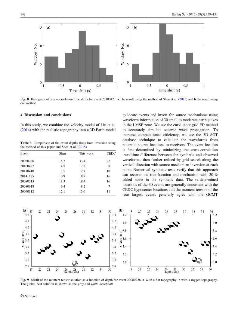
Fig. 8 Histogram of cross-correlation time shifts for event 20100427. a The result using the method of Shen et al. (2015) and b the result using

our method

Table 3 Comparison of the event depths (km) from inversion using

the method of this paper and Shen et al. (2015)

Event Shen This work CEDC

20080226 18.7 33.4 22

20100427 4.5 7.5 8

20110410 7.5 12.7 10

20141125 10.9 18.7 16

20080513 11.3 18.4 16

20080618 6.4 8.2 7

20090112 12.1 13.0 11

Fig. 9 Misfit of the moment tensor solution as a function of depth for event 20080226. a With a flat topography; b with a rugged topography.

The global best solution is shown as the grey-and-white beachball

148 Earthq Sci (2016) 29(3):139–151

123

solutions. We note that the synthetic waveforms from our

FD SGT method fit the observed better than those of

GCMT.

We analyze the effects of determining event locations

by cross-correlation traveltime difference. Compared to

Shen et al. (2015)’s amplitude-only approach, our depths

are closer to the results provided by CEDC and the cross-

correlation traveltime difference misfits are smaller,

indicating the positive effect of minimizing the cross-

correlation traveltime difference. We also investigate the

effect of the surface topography on source inversion. Most

source inversion studies adopt a flat topography to reduce

the difficulty of calculating SGT. This assumption may be

appropriate for regions with smooth terrains but is not

suitable for the LMSF zone. By comparing the inversion

results in models with and without the rugged topography

of the study region, we find that the source solutions in

the case with the topography provide a better fit to the

observed waveforms, especially on the vertical compo-

nent. The frequency band used in this study is not very

high due to the considerations of the computational cost

and the resolution of the reference model. At higher fre-

quencies, the effects of topography may be more pro-

nounced and should be more important in forward

simulation.

Our method can provide source mechanisms and event

locations of small to moderate earthquakes, which can be

further used in waveform-based tomography to refine the

3D Earth structure. Both earthquake source parameters and

velocity structures affect waveform traveltimes and should

be simultaneously or alternately updated in waveform-

based tomography. Our method could be an essential

component of a full-3D waveform tomography workflow to

provide earthquake locations and mechanisms toward

minimizing the cross-correlation traveltime and amplitude

misfits.

Fig. 10 Misfit of the moment tensor solution as a function of depth for event 20100427. a with a flat topography; b with a rugged topography.

The global best solution is shown as the grey-and-white beachball

Fig. 11 Misfit of the moment tensor solution as a function of depth for event 20110410. a With a flat topography; b with a rugged topography.

The global best solution is shown as the grey-and-white beachball

Earthq Sci (2016) 29(3):139–151 149

123

Acknowledgments We thank two anonymous reviewers for their

valuable peer-review comments and editors for their help, also thank

Earthquake Administration of Sichan Province, China for providing

the data. The comments of two anonymous reviewers and the help the

editors are gratefully acknowleged. This work is supported by

National Natural Science Foundation of China (Grants No. 41374056)

and the Fundamental Research Funds for the Central Universities

(WK2080000053).

Open Access This article is distributed under the terms of the

Creative Commons Attribution 4.0 International License (http://crea

tivecommons.org/licenses/by/4.0/), which permits unrestricted use,

distribution, and reproduction in any medium, provided you give

appropriate credit to the original author(s) and the source, provide a

link to the Creative Commons license, and indicate if changes were

made.

References

Aki K, Richards PG (2002) Quantitative Seismology. The 2nd edn.

University Science Books, Sausalito

Chen WP, Nabelek JL, Fitch TJ, Molnar P (1981) An intermediate

depth earthquake beneath Tibet: source characteristics of the

event of September 14, 1976. J Geophys Res 86:2863–2876

Chen P, Jordan TH, Zhao L (2007) Full three-dimensional tomog-

raphy: a comparison between the scattering-integral and adjoint-

wavefield methods. Geophys J Int 170(1):175–181

Chu R, Zhu L, Helmberger DV (2009) Determination of earthquake

focal depths and source time functions in central Asia using

teleseismic P waveforms. Geophys Res Lett 36(17)

Dreger D, Helmberger D (1991) Source parameters of the Sierra

Madre earthquake from regional and local body waves. Geophys

Res Lett 18(11):2015–2018

Dziewonski AM, Chou TA, Woodhouse JH (1981) Determination of

earthquake source parameters from waveform data for studies of

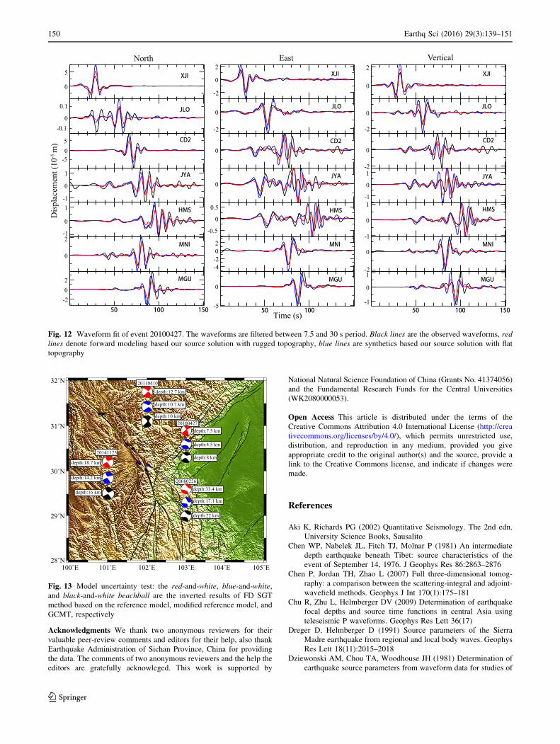
Fig. 12 Waveform fit of event 20100427. The waveforms are filtered between 7.5 and 30 s period. Black lines are the observed waveforms, red

lines denote forward modeling based our source solution with rugged topography, blue lines are synthetics based our source solution with flat

topography

100˚E 101˚E 102˚E 103˚E 104˚E 105˚E28˚N

29˚N

30˚N

31˚N

32˚N

20080226

20100427

20110410

depth:18.7 km

depth:17.1 km

depth:4.5 km

depth:10.7 km

depth:14.2 km

depth:22 km

depth:8 km

depth:10 km

depth:16 km

20141125

depth:12.7 km

depth:7.5 km

depth:33.4 km

Fig. 13 Model uncertainty test: the red-and-white, blue-and-white,

and black-and-white beachball are the inverted results of FD SGT

method based on the reference model, modified reference model, and

GCMT, respectively

150 Earthq Sci (2016) 29(3):139–151

123

global and regional seismicity. J Geophys Res

86(B4):2825–2852

Eisner L, Clayton RW (2001) A reciprocity method for multiple-

source simulations. Bull Seismol Soc Am 91(3):553–560

Ekstrom G, Engdahl ER (1989) Earthquake source parameters and

stress distribution in the Adak Island region of the central

Aleutian Islands, Alaska. J Geophys Res 94:15499–15519

Ekstrom G, Stein RS, Eaton JP, Eberhart-Phillips D (1992) Seismicity

and geometry of a 110-km-long blind thrust fault 1. The 1985

Kettleman Hills, California, earthquake. J Geophys Res

97:4843–4864

Ekstrom G, Nettles M, Dziewonski AM (2012) The global CMT

project 2004–2010: centroid-moment tensors for 13,017 earth-

quakes. Phys Earth Planet Interiors 200, 201:1–9. doi:10.1016/j.

pepi.2012.04.002

Gillard D, Rubin AM, Okubo P (1996) Highly concentrated

seismicity caused by deformation of Kilauea’s deep magma

system. Nature 384:343–346

Hardebeck JL, Shearer PM (2002) A new method for determining

first-motion focal mechanisms. Bull Seismol Soc Am

93:2434–2444

Hardebeck JL, Shearer PM (2003) Using S/P amplitude ratios to

constrain the focal mechanisms of small earthquakes. Bull

Seismol Soc Am 93(6):2434–2444

Hjorleifsdottir V, Ekstrom G (2010) Effects of three-dimensional

earth structure on CMT earthquake parameters. Phys Earth

Planet Inter 179:178–190

Kikuchi M, Kanamori H (1991) Inversion of complex body waves-III.

Bull Seismol Soc Am 81(6):2335–2350

Kisslinger C (1980) Evaluation of S to P amplitude ratios for

determining focal mechanisms from regional network observa-

tions. Bull Seismol Soc Am 70:999–1010

Klein FW (1994) Deep fault plane geometry inferred from multiple

relative relocation beneath the south flank of Kilauea. J Geophys

Res 99:15375–15386

Lee EJ, Chen P, Jordan TH, Wang L (2011) Rapid full-wave centroid

moment tensor (CMT) inversion in a three-dimensional earth

structure model for earthquakes in Southern California. Geophys

J Int 186(1):311–330

Liu Q, Polet J, Komatitsch D, Tromp J (2004) Spectral-Element

Moment Tensor Inversions for Earthquakes in Southern Cali-

fornia. Bull Seismol Soc Am 94(5):1748–1761

Liu QY, van der Hilst RD, Li Y, Yao HJ, Chen JH, Guo B, Qi SH,

Wang J, Huang H, Li SC (2014) Eastward expansion of the

Tibetan Plateau by crustal flow and strain partitioning across

faults. Nat Geosci 7(5):361–365

Nabelek JL (1984) Determination of earthquake source parameters

from inversion of body waves. Doctoral dissertation, Dept. of

Earth, Atmospheric and Planetary Sciences, MIT

Pei S, Su JR, Zhang HJ, Sun YS, Toksoz MN, Wang Z, Gao X, Jing

L-Z, He JK (2010) Three-dimensional seismic velocity structure

across the 2008 Wenchuan MS 8.0 earthquake, Sichuan, China.

Tectonophysics 491(1):211–217

Pettersen Ø, Doornbos DJ (1987) A comparison of source analysis

methods as applied to earthquakes in Tibet. Phys Earth Planet

Inter 47:125–136

Shearer PM (1997) Improving local earthquake locations using the L1

norm and waveform cross correlation: application to the Whittier

Narrows, California, aftershock sequence. J Geophys Res

102:8269–8283

Shen Y, Forsyth DW, Conder J, Dorman LM (1997) Investigation of

microearthquake activity following an intraplate teleseismic

swarm on the west flank of the Southern East Pacific Rise.

J Geophys Res 102:459–475

Shen Y, Zhang Z, Zhang W (2015) Moment inversions of earthquakes

in the southeast Tibetan plateau using finite-difference strain

Green tensor database, submitted to Geophys J Int

Tan Y, Helmberger D (2007) A new method for determining small

earthquake source parameters using short-period P waves. Bull

Seismol Soc Am 97(4):1176–1195

Thurber CH (1992) Hypocenter-velocity structure coupling in local

earthquake tomography. Phys Earth Planet Int 75(1):55–62

Tromp J, Tape C, Liu Q (2005) Seismic tomography, adjoint

methods, time reversal and banana-doughnut kernels. Geophys J

Int 160(1):195–216

Wang N, Shen Y, Ashton Flinders, Zhang W (2016) Accurate source

location from P waves scattered by surface topography, submit-

ted to J Geophys Res

Wu J, Ming Y, Wang C (2004) Source mechanism of small-moderate

earthquakes and tectonic stress field in Yunnan province. Acta

Seismol Sin 17:509–517

Yang Y, Ritzwoller MH, Zheng Y, Shen W, Levshin AL, Xie, Z

(2012) A synoptic view of the distribution and connectivity of

the mid-crustal low velocity zone beneath Tibet. J Geophys Res:

117(B4)

Zhang W, Chen X (2006) Traction image method for irregular free

surface boundaries in finite difference seismic wave simulation.

Geophys J Int 167(1):337–353

Zhang W, Shen Y (2010) Unsplit complex frequency-shifted PML

implementation using auxiliary differential equations for seismic

wave modeling. Geophysics 75(4):T141–T154

Zhang W, Shen Y, Zhao L (2012a) Three-dimensional anisotropic

seismic wave modelling in spherical coordinates by a collocated-

grid finite-difference method. Geophys J Int 188(3):1359–1381

Zhang W, Shen Y, Zhao L (2012b) Three-dimensional anisotropic

seismic wave modelling in spherical coordinates by a collocated-

grid finite-difference method. Geophys J Int 188(3):1359–1381

Zhang W, Zhang Z, Chen X (2012c) Three-dimensional elastic wave

numerical modelling in the presence of surface topography by a

collocated-grid finite-difference method on curvilinear grids.

Geophys J Int 190(1):358–378

Zhang Z, Zhang W, Chen X (2014) Complex frequency-shifted multi-

axial perfectly matched layer for elastic wave modelling on

curvilinear grids. Geophys J Int, ggu124

Zhao L-S, Helmberger DV (1994) Source estimation from broadband

regional seismograms. Bull Seismol Soc Am 84(1):91–104

Zhao L, Jordan TH, Olsen KB, Chen P (2005) Frechet kernels for

imaging regional Earth structure based on three-dimensional

reference models. Bull Seismol Soc Am 95(6):2066–2080

Zhao L, Chen P, Jordan TH (2006) Strain Green’s tensors, reciprocity,

and their applications to seismic source and structure studies.

Bull Seismol Soc Am 96(5):1753–1763

Zhu L, Helmberger DV (1996) Advancement in source estimation

techniques using broadband regional seismograms. Bull Seismol

Soc Am 86(5):1634–1641

Earthq Sci (2016) 29(3):139–151 151

123