location and characterization of emission sources for airborne volatile organic compounds inside a...

Environmental Monitoring and Assessment (2006) 120: 487–498

DOI: 10.1007/s10661-005-9076-6 c© Springer 2006

LOCATION AND CHARACTERIZATION OF EMISSION SOURCESFOR AIRBORNE VOLATILE ORGANIC COMPOUNDS INSIDE A

REFINERY IN TAIWAN

CHING-LIANG CHEN1, CHI-MIN SHU2 and HUNG-YUAN FANG2,∗1Doctoral Candidate, Graduate School of Engineering Science and Technology, National YunlinUniversity of Science and Technology (NYUST), 123, University Road, Section 3, Touliu, Yunlin,

Taiwan 640, Republic of China (R.O.C.); 2Professor, Department of Safety, Health andEnvironmental Engineering, NYUST, 123, University Road, Section 3, Touliu, Yunlin,

Taiwan 640, R.O.C.(∗author for correspondence, e-mail: [email protected])

(Received 13 July 2005; accepted 7 October 2005)

Abstract. This study aimed to locate VOC emission sources and characterized their emitted VOCs.

To avoid interferences from vehicle exhaust, all sampling sites were positioned inside the refinery.

Samples, taken with canisters, were analyzed by GC–MS according to TO-14 method. The survey

period extended from Febrary 2004 to December 2004, sampling twice per season. To interpret a

large number of VOC data was a rather difficult task. This study featured using ordinary application

software, Excel and Surfer, instead of expensive one like GIS, to overcome it. Consolidating data into

a database on Excel facilitated retrieval, statistical analysis and presentation in the form of either table

or graph. The cross analysis of the data suggested that the abundant VOCs were alkanes, alkenes,

aromatics and cyclic HCs. Emission sources were located by mapping the concentration distribution

of these four types of VOCs in terms of contour maps on Surfer. During eight surveys, five emission

sources were located and their VOCs were characterized.

Keywords: contour map, data interpretation, Excel, petrochemical plant, Surfer, survey, VOC

1. Introduction

VOCs emitted from refinery and petrochemical plants was another environmentalconcern second to vehicle exhausts (Srivastava et al., 2004). The VOCs concentra-tion from a petrochemical complex was reported 4–20 folds higher than those at asuburban site (Cetin et al., 2003; Corti et al., 2000; Na et al., 2001; Ostermark, 1995;Tsai et al., 1996; Kalabokas et al., 2001). It was pointed out that in a petrochemicalplant more than 80% of VOCs came from 20% equipment components. Therefore,locating emission sources is the first step to abate VOCs emissions (Siegell, 1998).

To locate the emission sources more quickly, the downwind concentrations wereinverted by an atmospheric dispersion model to reconstruct distribution (Lehninget al., 1994). PONG–2, a Gaussian plume modeling technique, was applied to mappossible odor sources (Tapper et al., 1991). Isopleths contour of concentration wasused to estimate emission sources and a large number of data were managed by

488 CHING-LIANG CHEN ET AL.

using database or Geographical Information System (GIS) (Jones et al., 1998; Liet al., 1995; Puliafito et al., 2003; Siegell, 1996).

In this paper, we surveyed airborne VOCs inside a large-sized refinery in Taoyan,Taiwan. To avoid the interference originated from vehicle exhausts, sampling wereconducted inside rather than outside the refinery. By combination of analytic ap-proach, database, and contour map, a total of five potential emission sources weretraced and their VOCs were characterized.

2. Experimental

2.1. SAMPLING

All units in this refinery could be categorized into five types including processunit, utility, tank farm, waste storage area section and surroundings. Each unit wasdeployed with one sampling site, whose position remained unchanged within thesurvey period. A total of 25 sampling sites were all positioned inside the plant, aslisted in Table I and depicted in Figure 1. Sampling height was about 1.5 m aboveground level, equivalent to that of a human nose. The survey period was one yearor so, extending from Febrary 2004 to December 2004. Sampling campaigns wereconducted twice per season. All procedures were based on the TO–14 methodrecommended by US EPA. Air was sampled with 6-L stainless steel canisters(Enteck, Inc., USA) whose interior wall was pre-coated with a layer of fused silicato ensure inertness to species. Each canister was fitted in the inlet with a flowrestrictor (CS 1200E Passive Sampler, Enteck, Inc., USA) to maintain a constantsampling rate of 33 ml/min. The sampling duration was three hours. In this way, itserved to level out the effects due to both wind speed and wind direction.

2.2. ANALYSIS

The analysis utilized a device called AUTOCAN (Tekmar, Inc., USA), which pos-sessed functions such as autosampling, cryoconcentration, thermodesorption, to-gether with cryofocusing, and an HP 5890 gas chromatograph (GC)/5971 mass se-lective detector (MS) (Hewlett Packard, Inc., USA). In preconcentration, a knownvolume (200 or 400 ml) of sample was drawn at flow rate of 65 ml/min regulatedby a mass flow regulator, through a stainless steel trap packed with CarbotrapC and Carbosieve, maintained at −50 ◦C by liquid nitrogen. The trapped VOCswere then thermally desorbed at 275 ◦C into a cryofocuser maintained at −180 ◦C,followed by heating to 200 ◦C to vaporize the condensed analytes into GC foranalysis.

The separation was performed on a DB-1 fused-silica capillary column (60 m× 0.32 mm × 1 μm, J & W Scientific, Inc., USA). The GC oven was initiallyheld at 5 ◦C for 4 min, then programmed to 200 ◦C at 6 ◦C/min and held for 5 min.

LOCATION AND CHARACTERIZATION OF EMISSION SOURCES 489

TABLE I

Sampling sites inside the refinery

Site No. Sampling site Typea

1 Tank farm-A B

2 Filling station A

3 Residue desulfur unit A

4 Tank farm-B B

5 Tank farm-C B

6 Tank farm-D B

7 Tank farm-E B

8 Isomerization unit-A A

9 Isomerization unit-B A

10 No. 2 Topping unit-A A

11 No. 1 Topping unit-A A

12 No. 1 Topping unit-B A

13 No. 1 Topping unit-C A

14 Gas oil desulfur unit A

15 No. 1 Hydrogen unit D

16 No. 2 Topping unit-B A

17 No. 2 Reforming unit A

18 No. 2 Alkylation unit-A A

19 No. 2 Alkylation unit-B A

20 No. 2 Alkylation unit-C A

21 Tank farm-F B

22 Tank farm-G E

23 Wastewater treatment unit C

24 Tank farm-H B

25 Side entrance E

aA: Process unit, B: Tank farm, C: Waste disposal area, D;

Utility, E: Surroundings.

The mass spectrometry was operated in electron impact (EI) and full scan mode,with its scan range within 34–200 amu. Precision, in terms of relative standarddeviation, was within 12% from seven replicate analyses of the calibration gasmixture at 10 ppb, and the method detection limit was about 0.1 ppb for a trappedsample volume of 400 ml. For more detail, please refer to the reports (Sin et al.,2001).

The certified gas standards, TO-14 and ozone precursor with each componentat nominal concentration of 1 ppm, were purchased from Resteck, Inc., USA. Thecalibration gas was prepared by static dilution. The response factor for each compo-nent was determined by analyzing 5 calibration gas mixtures at concentrations of


Figure 1. Sampling sites inside this refinary.

5, 10, 20, 50, 200 ppbv, respectively, for a trapped volume of 400 ml and thentaking their average. Concentration = peak area × response factor ÷ trappedvolume (ml).

2.3. DATABASE

The data obtained were all consolidated in a database on Microsoft Excel. Thedatabase contained fields such as plant name, sampling site, site number, site coor-dinate, sampling date, species, carbon number (Cn), pollutant type, response factor,concentration and concentration percentage, etc. The Excel provides some inherentfunctions, such as simple retrieval, conditional retrieval, cross analysis, statisticalanalysis and statistical plotting.

2.4. CONTOUR MAP

The data, including abscissa, ordinate and concentration, were acquired from adatabase according to retrieving conditions set by a user, and then copied into aSurfer worksheet (Golden Software, Inc., USA), which was subsequently trans-formed into a grad-file. In gridding, the concentrations of positions other than


sampling sites were worked out by statistical method through known concentrationsat sampling sites. The grid-file was again processed into contour lines. The map ofthe plant was finally loaded into Surfer and underlay the contour lines to combinewith each other into a contour map.

3. Results and Discussion

3.1. ABUNDANT VOCS

From cross analysis, as many as 173 species of VOCs emitted from inside this re-finery and could be categorized into a variety of types, such as alkanes, cyclic HCs(hydrocarbons), aromatics, alkenes, dienes, alkynes, aldehydes, ketones, ethers,esters, and halogenated hydrocarbons, as shown in Figure 2. The abudant VOCswere alkanes (51%), followed by alkenes (27%), aromatics (10%), cyclic HCs(8%), in decreasing order. Ostermark (1995) characterized the VOCs emittedfrom a Swedish cat-cracking unit inside a refinery and found the VOCs con-sisted of approximately 80% alkanes, 15–20% alkenes, 5% aromatics. It followedthat the most abundant VOCs in a refinery were alkanes, followed by alkenes,aromatics.

For a refinery, the feedstock is the crude oil, which consists of most alkanes, afew aromatics and cyclic HCs. Alkenes scarcely occur in crude oil, but are producedin the cracking units. Aromatics are produced in the reforming unit, which serve asimportant petrochemical basics as well as raw materials for gasoline of high octane-number. So far as a refinery is concerned, it is no wonder that airborne VOCs aremainly composed of alkanes, followed by aromatics or alkenes.

Figure 2. Percentage of each type of VOCs.


Figure 3. Contour maps on 02/27/2004 for alkanes, alkenes, aromatics, cyclic HCs.

3.2. LOCATING EMISSION SOURCES

In a refinery, the feedstock is usually a mixture instead of a single species and thus wetook account of only abundant VOCs in locating emission sources. Figure 3 displayscontour maps for alkanes, alkenes, aromatics and cyclic HCs on 02/27/2004, bywhich emission sources could be traced. In general, the denser the contour lineswere, the more greatly the concentration varied; in other word, in the center of agroup contour lines might hide an emission source. This was because the pollutants,once emitted, were mixed by air rapidly and their values drop fast with the distancefrom the emission source.

From the contour map for alkanes, two emission sources were located aroundSite 20 (No. 2 Alkylating unit-C), with peak concentration approximating 1,800ppb and around Site 6 (Tank farm-D), 500 ppb, respectively. The contour map foralkenes disclosed one emission source around Site 7 (Tank farm-E), whose peakconcentration approached 300 ppb. As for aromatics, three emissions were trackedaround Site 16 (No. 2 Topping unit-B), with peak concentration of 130 ppb, Site 20(No. 2 alkylating unit-C), 130 ppb, and Site 26 (Wastewater treatment unit), 90 ppb,respectively. Three emission sources for cyclic HCs were found and happened to


TABLE II

Emission sources found during eight surveys

Emission source Site covered VOCs type

No. 1 Topping unit 11,12,13 Alkanes, Aromatics, Alkenes, Cyclic HCs

No. 2 Topping unit 10,16 Alkanes, Aromatics, Cyclic HCs

No. 2 Alkylation unit 20 Alkanes, Cyclic HCs, Aromatics

Waste water treatment unit 23 Alkanes, Aromatics, Alkenes, Cyclic HCs

Tank Farm 6, 7 Alkanes, Alkenes, Cyclic HCs

be the same as the ones for aromatics; one around Site 16, with peak concentra-tion up to 280 ppb, another one around Site 20, 260 ppb, the last around Site 26,120 ppb.

In the same way, more emission sources could be traced from contour maps basedthe other surveys conducted on 03/13, 04/29, 06/18, 07/27, 08/31, 10/29, 12/19,respectively. Eventually, a total of nine emission sources were located during eightsurveys, as summarized in Table II. Thought nine emission sources were identified,some sites could be lumped together. According to the relevance of each other,Sites 6 and 7 were combined into Tank farm, Sites 10 and 16 into No. 2 Toppingunit and Sites 11, 12 and 13 into No. 1 Topping unit. As a result, nine emissionsources were lumped into five main sources.

3.3. OVERALL COMPARISON OF EMISSION SOURCES

The intensities for four main types of VOCs around five main emission sourcesduring eight surveys are depicted in Figure 4. Obviously, alkanes were predominantover other types. Of two heaviest emission sources, one situated around Wastewatertreatment unit, whose intensity up to 4,000 ppb or so, and another around Tank farm,3,200 ppb. Alkenes, highly active ozone precursors in the photochemical reaction,mostly emitted from Tank farm, whose intensity soared to 5,000 ppb, much higherthan that of other two ones, around No. 1 Topping unit and Wastewater treatmentunit, whose intensities were less than 450 ppb. Though less than the other types,aromatics were so high in toxicity that they were regulated by local EPA. Thesource around Wastewater treatment unit had a heaviest emission near to 360 ppbin intensity; the other three ones were all below 130 ppb. As for cyclic HCs, thesource still located around Wastewater treatment unit, whose intensity was four totwelve times higher than that of the others, approaching 1,400 ppb. Obviously, thesources around Wastewater treatment unit and Tank farm were much heavier thanother ones so that they should be remedied in preference.


Figure 4. Overall comparison of intensity of emission sources during eight surveys. Intensity refers

to the maximum of peak concentration for each source.

3.4. CHARACTERIZATION OF VOCS EMITTED FROM SOURCES

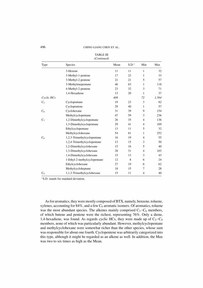
The characterization of VOCs from emission sources are summarized in Table III,where species with the maximum concentration less than 20 ppb are excluded be-cause of the limitation in content. By cross analysis of VOC database on Excel,we obtained mean concentration (Mean), standard deviation (S.D.), minimum con-centration (Min), maximum concentration (Max). The actually measured rangewas from Min to Max. On other hand, the sum of the maximum concentrationsmeant the heaviest emission in worst case. The statistical estimation, however,was more meaningful than the measured one. For example, the concentration ofa species may fall within Mean ± 1.645 S.D. in 90% probability. Taking tolueneas an example, it measured range fell within 30–194 ppb and statistically, within3–163 ppb in 90% probability. In the worst case, the aromatics might rise to 420 ppbor so.

Alkanes were most abundant, taking up about 50% of the total detected VOCspecies, and mainly consisted of C3 C10 members, including linear and branchedones. Alkanes were characterized by normal paraffin of C3 C10, such propane,butane, pentane, hexane, etc, accounting for 58% in terms of mean values. The fivemore plentiful species were propane, butane, 2-methylbutane, pentane, hexane, thesum of which was responsible for 71% of alkanes. It seemed that the lighter thespecies, the higher the mean concentration; this was mainly because lighter specieshad higher vapor pressure and tended to escaped from components of the processmore easily.


TABLE III

The characterization of VOCs emitted from sources inside the refinery (in ppb)

Type Species Mean S.D.∗ Min Max

Alkanes 1,743 278 7,058

C3 Propane 306 213 86 512

C4 Butane 256 264 6 874

Isobutane 81 71 18 207

C5 2-Methylbutane 361 696 38 2634

Pentane 201 236 16 933

2,3-Dimethylbutane 18 20 3 62

2-Methylpentane 82 86 20 284

3-Methylpentane 50 51 13 193

Hexane 117 124 34 508

C7 2,3-Dimethylpentane 8 10 2 36

2-Methylhexane 19 26 1 94

3-Methylhexane 22 24 1 90

Heptane 58 84 2 291

C8 2,3-Dimethylhexane 15 11 4 28

2-Methylheptane 32 21 11 66

3-Methylheptane 24 14 8 46

Octane 51 39 2 107

3-Methyloctane 13 10 6 20

C9 Nonane 19 16 4 51

C10 Decane 13 8 3 23

Aromatics 185 50 427

C6 Benzene 28 26 2 92

C7 Toluene 83 49 30 194

C8 m&p-Xylene 33 19 9 60

o-Xylene 12 6 4 23

C9 Ethyl-methyl-benzene isomers 13 8 3 26

Trimethyl-benzene isomers 16 10 3 32

Alkenes 1,162 118 5,692

C3 Propene 68 112 6 338

C4 2-Methylpropene 54 24 31 106

Butene 419 668 40 2,032

C5 Pentene 470 939 26 2,770

C6 2-Hexene 18 30 3 71

2-Methyl-1-pentene 15 27 1 64

(Continued on next page)


TABLE III

(Continued)

Type Species Mean S.D.∗ Min Max

3-Hexene 11 11 1 32



3-Methylenepentane 46 63 1 118


1,4-Hexadiene 13 20 1 37

Cyclic HCs 408 72 1,564

C5 Cyclopentane 19 23 3 82

Cyclopentene 29 40 1 57

C6 Cyclohexane 31 39 9 154

Methylcyclopentane 47 59 3 236

C7 1,2-Dimethylcyclopentane 26 35 4 136

1,3-Dimethylcyclopentane 29 41 4 169

Ethylcyclopentane 13 11 5 32

Methylcyclohexane 54 61 1 252

C8 1,2,3-Trimethylcyclopentane 16 19 4 55

1,2,4-Trimethylcyclopentane 13 15 3 50

1,2-Dimethylcyclohexane 15 16 5 40



1-Ethyl-2-methylcyclopentane 12 8 6 24

Ethylcyclohexane 27 19 6 62

Methylcycloheptane 18 15 7 28

C9 1,1,3-Trimethylcyclohexane 15 11 4 40

∗S.D. stands for standard deviation.

As for aromatics, they were mostly composed of BTX, namely, benzene, toluene,xylenes, accounting for 84%, and a few C9 aromatic isomers. Of aromatics, toluenewas the most abundant species. The alkenes mainly comprised C3 C6 members,of which butene and pentene were the richest, representing 76%. Only a diene,1,4-hexadiene, was found. As regards cyclic HCs, they were made up of C5 C9

members, none of which was particularly abundant. However, methylcyclopentaneand methylcyclohexane were somewhat richer than the other species, whose sumwas responsible for about one fourth. Cyclopentene was arbitrarily categorized intothis type, although it might be regarded as an alkene as well. In addition, the Maxwas two to six times as high as the Mean.


4. Conclusion

Samples taken inside a refinery could eliminate the interference from vehicle ex-hausts and ensured acquiring the authentic characterization of emitted VOCs. Theabudant VOCs in this refinery were found to be alkanes, alkenes, aromatics andcyclic HCs; this fact indicated the composition of airborne VOCs was consistentwith that of raw material, namely, crude oil, and the attribute of refining process. Bymapping these four types of VOCs, we located five main emission sources includ-ing No. 1, No. 2 Topping units, No. 2 Alkylation unit, Tank farm and Wastewatertreatment unit. Of them, Tank farm and Wastewater treatment unit were much sev-erer ones. The characterization of VOCs from sources was elucidated in terms ofmean concentration.

Acknowledgements

We greatly appreciate the Chinese Petroleum Corporation (CPC) in Taiwan forproviding financial assistance and experimental apparatus. We also thank the staffof the Environmental Engineering & Biotechnology Department in the CPC fortheir cooperation in sampling and routine tasks.

References

Cetin, E., Odabasi, M. and Seyfioglu, R.: 2003, ‘Ambient volatile organic compound (VOC) con-

centrations around a petrochemical complex and a petroleum refinery’, Sci. Tol. Environ. 312,

103–112.

Corti, A. and Senatore, A.: 2000, ‘Project of an air quality monitoring network for industrial site in

Italy’, Environ. Monit. Assess. 65(1–2), 109–117.

Jones, G., Gonzalez-Flesca, N., Sokh, R. S., McDonald, T. and Ma, M.: 1998, ‘Measurement and in-

terpretation of concentrations of urban atmospheric organic compounds’, Environ. Monit. Assess.52(1–2), 107–121.

Kalabokas, P. D., Hatzianestis, J., Bartzis, J. G. and Papagiannakopoulos, P.: 2001, ‘Atmospheric con-

centrations of saturated and aromatic hydrocarbons around a Greek oil refinery’, Atmos. Environ.35, 2545–2555.

Lehning, M., Chang, P. Y., Shonnard, D. R. and Bell, R. L.: 1994, ‘An inversion algorithm for

determining area–source emissions from downwind concentration measurements’, J. Air & WasteManage. Assoc. 44(10), 1204–1213.

Li, R., Karell, M. and Boddy, J. W.: 1995, ‘Develop a plantwide air emissions inventory’, Chem. Eng.Prog. March, 96–103.

Na, K., Kim, Y.P., Moon, K.C., Moon, I. and Fung, K.: 2001,. ‘Concentrations of volatile organic

compounds in an industrial area of Korea’, Atmos. Environ. 35, 2747–2756.

Ostermark, U.: 1995, ‘Characterization of volatile hydrocarbons emitted to air from a cat-cracking

pefinery’, Chemosphere 30 9, 1813–1817.

Puliafito, E., Guevara, M. and Puliafito, C.: 2003, ‘Characterization of urban air quality using GIS as

a management system’, Environ. Pollut. 122, 105–117.


Siegell, J. H.: 1996, ‘Solve plant odor problems’, Chem. Eng. Prog. January, 35–41.

Siegell, J. H.: 1998, ‘Monitor your fugitive emissions correctly’, Chem. Eng. Prog. November, 33–38.

Sin, D. W., Wong, Y. C., Sham, W. C. and Wang, D.: 2001, ‘Development of an analytical technique

and stability evaluation of 143 C3 C12 volatile organic compounds in summa canisters by gas

chromatography/mass spectrometry’, Analyst 126, 310–321.

Srivastava, A. Joseph, A. E. and Wachasunder, S. D.: 2004, ‘Qualitative detection of volatile organic

compounds in outdoor and indoor air’, Environ. Monit. Assess. 96(1–3), 263–271.

Tapper, N. J. and Sudbury, A. W.: 1991, ‘Mapping odor sources from complaint statistics I: identifying

the major source’, J. Air & Waste Manage. Assoc. 41, 433–441.

Tsai, J. H., Sheu, Y. C., Lee, D. Z. and Lin, S. J.: 1996, ‘Airborne aromatic volatile organics in the

vicinity of a refinery complex during operation and hot–standby modes’, J. Environ. Sci. HealthA 31(2), 463–477.

location and characterization of emission sources for airborne volatile organic compounds inside a...

Documents