Locating Sparse Solutions of

Underdetermined Linear Systems via theReweighted ℓ1-Method

Yunbin ZHAO and Duan LI

School of Matheamtics, University of Birmingham, United Kingdomhttp://web.mat.bham.ac.uk/Y.Zhao(E-mail: y.zhao.2@bham.ac.uk)

March, 2012

Outline

◮ Introduction

◮ Reweighted algorithm framework

◮ Convergence

◮ Numerical performance

◮ Conclusions

Introduction: ℓ0-problem

◮ Many data types (e.g. signal and image processing) can be

sparsely represented.

◮ Processing tasks handling such data

◮ Compression◮ Reconstruction◮ Storing◮ Separation◮ Transmission◮ ...

often amount to the problem:

(ℓ0) Minimize {‖x‖0 : Ax = b},

where A is an m × n matrix with m < n.

Introduction: ℓ1-problem

◮ ℓ0-problem is an NP-hard discrete optimization problem

[Natarajan, 1995].

◮ ℓ1-norm, i.e.,

‖x‖1 =n

∑

i=1

|xi |,

is the convex envelope of ‖x‖0 over the region ‖x‖∞ ≤ 1.

◮ Replacing ‖x‖0 by ‖x‖1 yields the ℓ1-minimization:

(ℓ1) Minimize {‖x‖1 : Ax = b},

which is identical to a linear programming (LP) problem.

When does ℓ1- solves ℓ0-minimization?

Conditions for the matrix A under which ℓ0-problem is

computationally tractable:

◮ Spark and Mutual Cohence [Donoho and Elad (2003)]

◮ Restricted Isometry Property (RIP) [Candes and Tao (2005)]

◮ Null Space Property (NSP) [Cohen et al (2009), Zhang

(2008), etc.]

◮ Verifiable conditions (Juditski and Nemirovski (2011)]

◮ Range Space Property [Zhao (2012a, 2012b)]

Introduction: Reweighted ℓ1-minimization

Reweighted ℓ1-minimization)

S1. Choose x0 ∈ Rn be an initial point.

S2. Define the weight wk which is determined by xk . Then

xk+1 = argmin{‖W kx‖1 : Ax = b},

where W k = diag(wk).

S3. Use xk+1 to define W k+1 Repeat S2.

Numerical experiments indicate that the reweighted

ℓ1-minimization does outperform ℓ1-minimization in many

situations [Candes, et al (2008), ...]

Examples: Reweighted ℓ1-minimization

◮ (Candes, Wakin and Boyd (2008) ) The method (CWB) with

wki =

1

|xki |+ ε, i = 1, ..., n,

◮ (Foucart and Lai (2009), etc) Weight

wki =

1

(|xki |+ ε)1−p, i = 1, ..., n, (1)

where p ∈ (0, 1) is a given parameter,

The understanding of reweighted ℓ1-minimization remains very

incomplete so far. Even the convergence property of the CWB

algorithm remains unclear at present.

A unified framework of reweighted ℓ1-method

Definition. A function from Rn to R is said to be a merit function

for sparsity if it is an approximation to ‖x‖0 in some sense.

Examples:

◮ ‖x‖1. (convex approximation of ‖x‖0 over ‖x‖∞ ≤ 1)

◮ ‖x‖p , p ∈ (0, 1). (‖x‖pp → ‖x‖0 as p → 0)

◮ There exist a vast number of merit functions for sparsity.

Minimizing such a function may drive the variable x to

become sparse when a sparse solution exists.

◮ From a computational point of view, a merit function for

sparsity should admit certain desired properties such as

convexity or concavity.

A unified framework of reweighted ℓ1-method

Separable concave merit functions:

◮

F (x) =n

∑

i=1

φi (|xi |),

where φi : R+ → R is called the kernel function.

◮ Replacing |xi | by |xi |+ ε where ε > 0 yields

min

{

Fε(x) =

n∑

i=1

φi (|xi |+ ε) : Ax = b

}

.

Notation:◮ For a subset S ⊆ {1, ..., n}, F (xS ) is the reduced function,

F (xS ) :=∑

i∈S φi (|xi |).◮ f : Rn → R+ is said to be coercive in the region D ⊆ Rn if

f (x) → ∞ as ‖x‖ → ∞ and x ∈ D.

A unified framework

For any given ε > 0, consider the merit function Fε : Rn → R

satisfies all the following properties:

Assumption:

(a) Fε(x) = Fε(|x |) for any x ∈ Rn, and Fε(x) is separable in x ,

and twice continuously differentiable with respect to x ∈ Rn+.

(b) In Rn+, Fε(x) is strictly increasing with respect to every

component xi and ε, and for any given γ > 0 there exists a

finite number Q(γ) such that for any S ⊆ {1, ..., n},

g(xS ) := infε↓0 Fε(xS ) ≥ Q(γ) provided xS ≥ γeS , and g(xS )

is coercive in the set {xS : xS ≥ γeS}.

Assumption (continued)

(c) In Rn+, the gradient satisfies that ∇Fε(x) ∈ Rn

++ for any

(x , ε) ∈ Rn+ × R++, [∇Fε(x)]i → ∞ as (xi , ε) → 0, and for

any given xi > 0 the component [∇Fε(x)]i is continuous in ε

and tends to a finite positive number as ε → 0.

(d) In Rn+, the Hessian satisfies that yT∇2Fε(x)y ≤ −C (ε, r)‖y‖2

for any y ∈ Rn and x ∈ Rn+ with ‖x‖ ≤ r , where r > 0 and

C (ε, r) > 0 are constants, and C (ε, r) is continuous in ε and

bounded away from zero as ε → 0.

A unified framework

The class M of merit functions:

M = {Fε : Fε satisfies the assumption above for ε > 0}.

Problem:

min

{

Fε(x) =

n∑

i=1

φi (|xi |+ ε) : Ax = b

}

. (2)

◮ For any Fε ∈ M, (2) can be rewritten as

min{Fε(v) : Ax = b, |x | ≤ v} = min(x ,v)∈F

Fε(v), (3)

where

F = {(x , v) : Ax = b, |x | ≤ v}.

How to handle (2)?

Linearization:

◮ Given the current point vk ,

Fε(v) = Fε(vk) +∇Fε(v

k)T (v − vk) + o(‖v − vk‖).

◮ Thus it makes sense to solve the following problem to

generate the next point (xk+1, vk+1) :

(xk+1, vk+1) = arg min(x ,v)∈F

{

Fε(vk) +∇Fε(v

k)T (v − vk)}

= arg min(x ,v)∈F

∇Fε(vk)T v (4)

which is a linear programming (LP) problem.

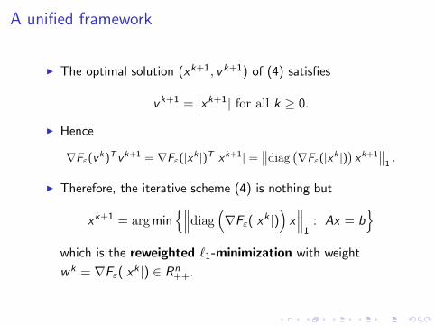
A unified framework

◮ The optimal solution (xk+1, vk+1) of (4) satisfies

vk+1 = |xk+1| for all k ≥ 0.

◮ Hence

∇Fε(vk )T vk+1 = ∇Fε(|x

k |)T |xk+1| =∥

∥diag(

∇Fε(|xk |)

)

xk+1∥

∥

1.

◮ Therefore, the iterative scheme (4) is nothing but

xk+1 = argmin{∥

∥

∥diag

(

∇Fε(|xk |)

)

x∥

∥

∥

1: Ax = b

}

which is the reweighted ℓ1-minimization with weight

wk = ∇Fε(|xk |) ∈ Rn

++.

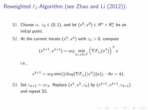
Reweighted ℓ1-Algorithm (see Zhao and Li (2012)):

S1. Choose α, ε0 ∈ (0, 1), and let (x0, v0) ∈ Rn × Rn+ be an

initial point.

S2. At the current iterate (xk , vk) with εk > 0, compute

(xk+1, vk+1) = arg min(x ,v)∈F

(

∇Fεk (vk))T

v

i.e.,

xk+1 = argmin{‖diag(∇Fεk (|xk |))x‖1 : Ax = b}.

S3. Set εk+1 = αεk . Replace (xk , vk , εk) by (xk+1, vk+1, εk+1)

and repeat S2.

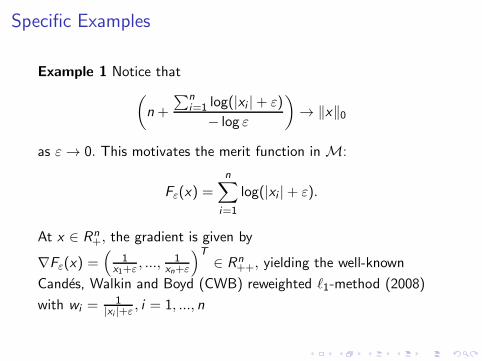
Specific Examples

Example 1 Notice that

(

n+

∑ni=1 log(|xi |+ ε)

− log ε

)

→ ‖x‖0

as ε → 0. This motivates the merit function in M:

Fε(x) =

n∑

i=1

log(|xi |+ ε).

At x ∈ Rn+, the gradient is given by

∇Fε(x) =(

1x1+ε , ...,

1xn+ε

)T

∈ Rn++, yielding the well-known

Candes, Walkin and Boyd (CWB) reweighted ℓ1-method (2008)

with wi =1

|xi |+ε , i = 1, ..., n

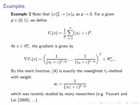
Examples

Example 2 Note that ‖x‖pp → ‖x‖0 as p → 0. For a given

p ∈ (0, 1), we define

Fε(x) =1

p

n∑

i=1

(|xi |+ ε)p .

At x ∈ Rn+, the gradient is given by

∇Fε(x) =

(

1

(x1 + ε)1−p, ...,

1

(xn + ε)1−p

)T

∈ Rn++.

By this merit function, (4) is exactly the reweighted ℓ1-method

with weight

wi =1

(|xi |+ ε)1−p

which was recently studied by many researchers (e.g. Foucart and

Lai (2009), ...).

Examples

Example 3 Let p ∈ (0, 1). It is easy to verify that the following

function is in M :

Fε(x) =n

∑

i=1

log (|xi |+ ε+ (|xi |+ ε)p) .

This merit function yields a reweighted ℓ1-algorithm with the

following weight:

wi = [∇Fε(|x |)]i =p + (|xi |+ ε)1−p

(|xi |+ ε)1−p [|xi |+ ε+ (|xi |+ ε)p], i = 1, ..., n,

which has not been studied in the literature.

Examples

Example 4

Let p and q ∈ (0, 1) be given. Define

Fε(x) =1

p

n∑

i=1

(|xi |+ ε+ (|xi |+ ε)q)p ,

which is in M. The gradient of this function at x ∈ Rn+ is given by

[∇Fε(x)]i =q + (xi + ε)1−q

(xi + ε)1−q [xi + ε+ (xi + ε)q]1−p, i = 1, ..., n.

Examples

Example 5

Then the following function remains in M :

Fε(x) =1

p

n∑

i=1

(

|xi |+ ε+ (|xi |+ ε)2)p

.

The associated reweighted ℓ1-minimization with

wi = [∇Fε(|x |)]i =1 + 2(|xi |+ ε)

(|xi |+ ε+ (|xi |+ ε)2)1−p, i = 1, ..., n

is also a new algorithm.

Examples

Example 6

Fε(x) =n

∑

i=1

[

log(|xi |+ ε)−1

(|xi |+ ε)p

]

(5)

The associated reweighted ℓ1-minimization uses the weight:

wi =1 + (|xi |+ ε)p

(|xi |+ ε)p+1, i = 1, ..., n.

Convergence of Algorithm (see Zhao and Li (2012))

Definition (Rang Space Property (RSP)).

Let A be an m × n matrix with m ≤ m. AT is said to satisfy the

range space property of order K with a constant ρ > 0 if

‖ξSc‖1 ≤ ρ‖ξS‖1

for all sets S ⊆ {1, ..., n} with |S | ≥ K , and for all ξ ∈ R(AT ), the

range space of AT .

Related to existing conditions:

◮ Restricted Isometry Property (RIP) [Candes and Tao(2005]: A

has the RIP of order k if there exists a constant δ ∈ (0, 1)

such that

(1− δ)‖z‖2 ≤ ‖Az‖2 ≤ (1 + δ)‖z‖2

for any k-sparse vector z ∈ Rn.

◮ Null Space Property (NSP) [Cohen et al (2009), Zhang

(2008),..]: A has the NSP of order k if there exists a constant

τ ∈ (0, 1) such that

‖ηS‖1 ≤ τ‖ηSc‖1

for all the sets S ⊆ {1, ..., n} with |S | ≤ k , and any

η ∈ N (A), the null space of A.

Relationship of RSP, RIP and NSP

Proposition Let m < n, and let A ∈ Rm×n and M ∈ R (n−m)×n be

full-rank matrices satisfying AMT = 0. Then the following holds:

◮ M has the NSP of order k with constant τ ∈ (0, 1) if and only

if AT has the RSP of order (n − k) with the same constant

ρ = τ.

◮ If M has the RIP of order k with constant δ ∈ (0, 1), then AT

has the RSP of order(

n− ⌊ k1+⌋

)

with the constant

ρ =

(

⌊ k1+

⌋

k−⌊ k1+

⌋

)1/2(

1

)

< 1 where = (1− δ)/(1 + δ).

Theorem 4.8. Let A ∈ Rm×n with m ≤ n, and assume that AT

has the RSP of order K with constant ρ > 0 satisfying 1 + ρ < nK.

Let Fε ∈ M and {(xk , vk)} be generated by Algorithm 3.2. Then

[σ(xk )]n = min1≤i≤n

|xki | → 0 as k → ∞. (6)

Theorem 4.10. Let A ∈ Rm×n with m ≤ n. Assume that AT has

the RSP of order K with constant ρ > 0 satisfying 1 + ρ < nK. Let

Fε ∈ M and the sequence {(xk , vk)} be generated by Algorithm

3.2. If ‖vk+1 − vk‖ → 0 as k → ∞, then there is a subsequence

{xkj } that converges to a ⌊(1 + ρ)K⌋-sparse solution of Ax = b in

the sense that [σ(xkj )]⌊(1+ρ)K+1⌋ → 0 as j → ∞.

Theorem 4.12. Assume that AT has the RSP of order K with

constant ρ > 0 satisfying that 1 + ρ < nK. Let Fε ∈ M and Fε(v)

be bounded below in (x , v) ∈ Rn+ × R+ and g(x) = infε↓0 Fε(x) be

coercive in Rn+. Let {(x

k , vk)} be generated by Algorithm 3.2.

Then there is a subsequence {xkj } that converges to a

⌊(1 + ρ)K⌋-sparse solution of Ax = b in the sense that

[σ(xkj )]⌊(1+ρ)K+1⌋ → 0 as j → ∞.

Numerical Experiments

The following reweighted algorithms were compared:

(a) Candes-Wakin-Boyd (CWB) method:

xk+1 = arg min

{

n∑

i=1

(

1

|xki |+ εk

)

|xi | : Ax = b

}

.

(b) ‘Wlp ’ method :

xk+1 = argmin

{

n∑

i=1

(

1

(|xki |+ εk)1−p

)

|xi | : Ax = b

}

, p ∈ (0, 1).

(c) ‘NW1’ algorithm derived from Example 3.3(ii):

xk+1 = argmin

{

n∑

i=1

(

p + (|xki |+ εk)

1−p

(|xki |+ εk)1−p

[

|xki |+ εk + (|xk

i |+ εk)p]

)

|xi | : Ax = b

}

where p ∈ (0, 1).

(d) ‘NW2’ algorithm derived from Example 3.5:

xk+1 = argmin

{

n∑

i=1

(

q + (|xki |+ εk)

1−q

(|xki |+ εk)1−q

[

|xki |+ εk + (|xk

i |+ εk)q]1−p

)

|xi | : Ax = b

where p, q ∈ (0, 1).

(e) ‘NW3’ algorithm derived from Example 3.5 (p ∈ (0, 1/2]):

xk+1 = argmin

{

n∑

i=1

(

1 + 2(|xki |+ εk)

(|xki |+ εk + (|xk

i |+ εk)2)1−p

)

|xi | : Ax = b

}

.

(f) ‘NW4’ algorithm based on Example 3.6(p ∈ (0,∞):

xk+1 = argmin

{

n∑

i=1

(

1 + (|xki |+ εk)

p

(|xki |+ εk)1+p

)

|xi | : Ax = b

}

.

Numerical Experiments

◮ Randomly generate (A, x) where A ∈ R50×250, and x is a

k-sparse vector in R250, and k = 1, 2, ..., 30.

◮ Based on the following assumption: The entries of A and x on

its support are i.i.d Gaussian random variables with zero mean

and unit variances.

◮ For every given sparsity k , 500 pairs of (A, x) were generated.

◮ Every reweighted algorithm was executed only 4 iterations,

and α = 0.5, ε0 = 0.01 and x0 = e ∈ R250 were used in

Algorithm 3.2.

◮ Given a k-sparse solution x , the algorithm claims to be

successful in finding the k-sparse solution x if the found

solution xk satisfies that ‖xk‖0 ≤ k and ‖xk − x‖ ≤ 10−5.

‖xk‖0 is the number of components of x satisfying

|xki | ≥ 10−5.

Numerical Experiments

0 5 10 15 20 25 300

10

20

30

40

50

60

70

80

90

100

k−sparsity

Freq

uenc

y of e

xact

reco

nstru

ction

l1−minCWBWlpNW1NW2NW3NW4

(a) p = 0.5

0 5 10 15 20 25 300

10

20

30

40

50

60

70

80

90

100

k−sparsity

Freq

uenc

y of e

xact

reco

nstru

ction

l1−minCWBWlpNW1NW2NW3NW4

(b) p = 0.3

Numerical Experiments

0 5 10 15 20 25 300

10

20

30

40

50

60

70

80

90

100

k−sparsity

Freq

uenc

y of

exa

ct re

cons

truct

ion

l1−minCWBWlpNW2

(a) p = 0.7

0 5 10 15 20 25 300

10

20

30

40

50

60

70

80

90

100

k−sparsity

Freq

uenc

y of

exa

ct re

cons

truct

ion

l1−minCWBWlpNW2

(b) p = 0.3

0 5 10 15 20 25 300

10

20

30

40

50

60

70

80

90

100

k−sparsity

Freq

uenc

y of

exa

ct re

cons

truct

ion

l1−minCWBWlpNW2

(c) p = 0.1

0 5 10 15 20 25 300

10

20

30

40

50

60

70

80

90

100

k−sparsity

Freq

uenc

y of

exa

ct re

cons

truct

ion

l1−minCWBWlpNW2

(d) p = 0.01

Numerical Experiments

It is interesting to test algorithms using a different parameter

updating rule.

Candes, Wakin and Boyd (2008) proposed the following rule:

εk = max{

[σ(xk)]i0 , 10−3

}

,

where i0 denotes the nearest integer to m/[4 log(n/m)].

Numerical Experiments

0 5 10 15 20 25 300

10

20

30

40

50

60

70

80

90

100

k−sparsity

Freq

uenc

y of

exa

ct re

cons

truct

ion

l1−minCWBWlpNW1NW2NW3NW4

(i) p = 0.5, εk is updated by (32)

0 5 10 15 20 25 300

10

20

30

40

50

60

70

80

90

100

k−sparsity

Freq

uenc

y of

exa

ct re

cons

truct

ion

l1−minCWBWlpNW1NW2NW3NW4

(ii) p = 0.3, εk is updated by (32)

Conclusions

◮ Through the linearization technique, minimizing the concave

merit functions for sparsity yields a unified approach for the

reweighted ℓ1-minimization algorithms.

◮ By this unified approach, we can construct various new

specific reweighted ℓ1-algorithms for the sparse solution of

linear systems, and develop a new and unified convergence

theory for a large family of these algorithms.

◮ Our convergence analysis is based on the Range Space

Property (RSP), which is different from the existing

RIP/NSP-based analysis.

◮ As special cases of our general framework, a convergence

result for the well-known ℓp-quasi-norm-based algorithm and

Candes-Wakin-Boyd method can be obtained.

Conclusions (continued)

◮ We have proved that, under suitable conditions, a large family

of reweighted ℓ1-algorithms can generate a solution with

certain level of sparsity to the linear system.

◮ Although the simulation shows that reweighted ℓ1-algorithms

outperform the standard ℓ1-method in many situations, a

rigorous mathematical proof for this phenomena has not been

carried out so far. This remains an open question in this field.

Key References

E.J. Candes, M.B. Wakin and S.P. Boyd, Enhancing sparsity byreweighted ℓ1 minimization, J. Fourier Anal. Appl., 14 (2008), pp.877-905.

S. Foucart and M.J. Lai, Sparsest solutions of underdeterminedlinear systems via ℓp-minimization for 0 < q ≤ 1, Applied and

compational Harmonic Analysis, 26 (2009), pp. 395-407.

Y.B. Zhao and D. Li, Reweighted ℓ1-minimization for sparsesolutions of underdetermined linear systems, SIAM J. Optim, 22(2012), no.3, pp. 1065-1088.

Y.B. Zhao, RSP-Based Analysis for Sparsest and Least ℓ1-NormSolutions to Underdetermined Linear Systems, Technical report,University of Birmingham, 2012.

Y.B. Zhao, Equivalence and Strong Equivalence between theSparsest and Least l1-Norm Nonnegative Solutions of Linear Systemsand Their Applications, Technical report, University of Birmingham,2012.