locally generated surface waves in santa clara valley: analysis of observations and numerical...

EARTHQUAKE ENGINEERING AND STRUCTURAL DYNAMICS, VOL. 25,47-63 (1996)

LOCALLY GENERATED SURFACE WAVES IN SANTA CLARA VALLEY: ANALYSIS OF OBSERVATIONS AND NUMERICAL

SIMULATION

DUOLI PEI AND APOSTOLOS S. PAPAGEORGIOU Department of Civil Engineering, Rensselaer Polytechnic Institute, Troy, New York 12180-3590, US.A

SUMMARY The motions recorded by the Gilroy array of instruments on the surface of the Santa Clara Valley, California, during the 1989 Loma Prieta and 1984 Morgan Hill earthquakes are analysed for evidence of oalley induced surface waves.

The Santa Clara Valley extends in a NW-SE direction, south of the San Francisco Bay. The Gilroy linear array of instruments is an east-west alignment of stations crossing the Santa Clara Valley. Seismic refraction studies in the vicinity of the array indicate that the valley is wedge-shaped in cross-section with maximum thickness of the order of 1 km.

Analysis of the recorded motions of the 1989 Loma Prieta earthquake reveal clear evidence of the fundamental and first and second higher modes of Rayleigh waves, while analysis of the recorded motions of the 1984 Morgan Hill earthquake shows, in addition to the above surface wave modes, the presence of the fundamental Love mode. Motions generated by the latter event were more complicated due to the presence of the low-velocity zone of the Calaveras fault, which traps and focuses seismic energy generated by slip on the fault, and leaks it to the surrounding medium in a rather complicated manner.

The observed valley-induced surface waves are simulated using a hybrid numerical technique which combines the Boundary Integral Equation Method with the Finite Element Method. The mathematical formulation that we use has been developed for a class of cylindrical inclusions of infinite length, having an arbitrary cross-section, embedded in a homogeneous (or layered) half-space, subjected to plane waves impinging at an oblique angle with respect to the axis of the inclusion. Even though the model of the valley is two-dimensional, the response is three-dimensional and has the particular feature of repeating itself with a certain delay for different observers along the axis of the valley. This feature leads to a considerably simpler solution than that for a valley with a 3-D geometry.

KEY WORDS: basin response; surface waves; earthquake engineering; seismology

INTRODUCTION

Following the seminal works of Aki and Larner,’ Boore et al.,’ and T r i f ~ n a c , ~ there has been considerable interests in the effects that sedimentary deposits, in the form of basins, valleys or alluvial fans, have on earthquake ground motions. Many theoretical and observational studies on ‘basin effects’ have been reported in the published literature since then (e.g. References 423) .

It is now well-established that sedimentary valleys are effective in trapping and focusing energy, thus increasing peak amplitudes, and extending the duration of motion. Specifically, the efficient trapping of incident S-wave energy within the alluvium is caused by the downward and away from the source slope of the alluvium-bedrock interface. As the transmitted-to-the-sediment S-wave energy is multiply reflected by the free surface, it has an increasingly grazing angle of incidence at the alluvium-bedrock interface. Eventually, this transmitted and multiply reflected S-wave energy is critically reflected within the alluvium, thus becoming surface waves which propagate across the valley, prolonging the duration of motion (e.g. References 6,22 and 24). A clear visualization of the surface wave generation process described above may be found in Ohtsuki et al.25*26

For irregularly shaped basins, observational evidence and 3-D modelling (e.g. References 16,27, 18, 19 and 23), have demonstrated that the S-to-surface wave conversion could occur along several portions of the basin border, producing surface waves travelling in different directions across the basin.

CCC 0098-8847/96/010047-17 0 1996 by John Wiley & Sons, Ltd.

Receiced 23 February 1995 Revised 1 August 1995

48 D. PEI AND A. S. PAPAGEORGIOU

However, in many cases, basins or valleys as they occur in nature, by virtue of their formation process, are elongated bodies of sediments, usually bounded by faults which run parallel to their axis. As examples, we mention the basin of the San Francisco Bay and the Santa Clara Valley at the vicinity of Gilroy, both bounded by the San Andreas fault to the west and the Calaveras fault to the east. In such cases, and for all practical purposes, valleys can be modelled as 2-D scatterers for which the S-to-surface wave conversion occurs along the two parallel edges. In order for such a model to have a wide range of applications, its mathematical formulation must accommodate seismic energy incident from any azimuthal direction, and not only from a direction normal to the axis of the 2-D scatterer, as it is the case for standard 2-D modelling.

In this paper we analyse the response of the Santa Clara Valley to the 1989 Loma Prieta and 1984 Morgan Hill earthquakes, recorded by the linear Gilroy array which crosses the valley. We model the response using a hybrid numerical method which combines the Boundary Integral Equation Method with the Finite Element Method. The formulation that we use has been developed for a class of cylindrical inclusions of infinite length, having an arbitrary cross-section, embedded in a homogeneous (or layered) half-space, and subjected to plane waves impinging at an oblique angle with respect to the axis of the inclusion (Zhang et ~ 1 . ' ~ ; a manuscript is in preparation which will present in detail the above-mentioned hybrid numerical technique). Even though the model of the scatterer is two-dimensional, the response is three-dimensional and has the particular feature of repeating itself with a certain delay for different observers along the axis of the scatterer. This feature leads to a considerably simpler solution than that for a scatterer with a 3-D geometry.

Three-dimensional scattering by 2-D scatterers has been studied by Khair et Luco et u Z . , ~ ' Zhang and C h ~ p r a , ~ ' Pei and Papage~rgiou,~' Pedersen et al.,j3 and Luco and de B a r r ~ s . ~ ~

The motivation for the present study is to present additional observational evidence of the valley-induced (or locally generated) surface waves, and to investigate potential variations of valley response as a function of the earthquake location relative to the scatterer/valley (Jongmans and Campil10~~). These valley-induced surface waves have important implications for the aseismic design of long period structures such as high-rise buildings, long-span bridges and base isolated structures.

THE GILROY STRONG-MOTION ARRAY

The Gilroy strong-motion array is a northeast-southwest alignment of stations crossing the Santa Clara Valley (Figure 1). This array is a cooperative effort of the California Division of Mines and Geology (CDMG) Strong Motion Instrumentation Program (CSMIP) and the U.S. Geological Survey Branch of Engineering Seismology and Geology, and is currently instrumented and maintained by CSMIP. The array, extending 10 km from Franciscan rocks on the southwest across Quaternary alluvium of the Santa Clara Valley to Crataceous rocks of the Great Valley sequence on the northeast, provided significant records of the 1979 Coyote Lake e a r t h q ~ a k e , ~ ~ 1984 Morgan Hill earthquake3' and 1989 Loma Prieta ear thq~ake .~ '

Seismic refraction studies of the Santa Clara Valley near the Gilroy array were performed and reported by Mooney and L ~ e t g e r t ~ ~ and Mooney and C ~ l b u r n . ~ ' Interpretation of the data indicates that the valley is wedge-shaped in cross-section with the basement dipping 10" to the northeast beneath the Quaternary alluvium of the valley. This agrees quite well with the 7" dip computed from the depth to Franciscan rock at station 2 and the distance to the edge of the alluvium (Joyner et ~ 1 . ~ ' ) . It is also consistent with the dip of approximately 14" northeast that characterizes the exposed Franciscan surface southwest of the valley. Of the two refraction profiles, one southeast of the array and the other northwest of it (Figure l), the former indicates a maximum thickness of 1.5 km for the alluvial fill, while the latter shows a maximum thickness of 1.0 km. The data show an average P-wave velocity of 2.3 km/s for the alluvial fill and 4.3 km/s for the top of the basement; the P-wave velocity reaches 6.0 km/s at a depth of 2 km.

ANALYSIS OF RECORDED RESPONSE OF THE SANTA CLARA VALLEY

The 1989 Loma Prieta, California, earthquake The 18 October 1989 Loma Prieta earthquake ( M , = 7.1; ML = 6-9) provided one of the most complete

sets of near-source strong records ever, and has been the subject of numerous source inversion s t ~ d i e s . ~ ' - ~ ~

LOCALLY GENERATED SURFACE WAVES 49

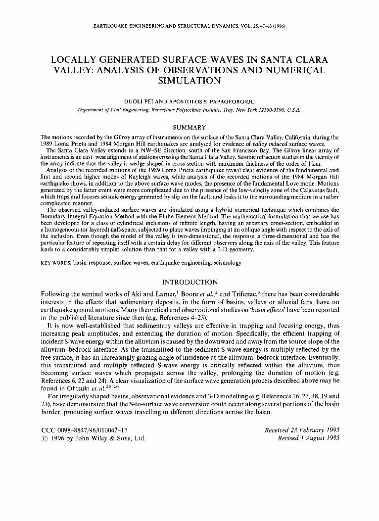
Figure 1. Geologic map of Santa Clara Valley in the vicinity of the Gilroy array. The southeast segment of the fault, that generated the 1989 Loma Prieta earthquake, projected on the horizontal surface of the earth, is indicated by a rectangle. The epicenter of the earthquake is indicated by the star, while the southern compact area of major slip discussed in the text is indicated by concentric circles. The locations of seismic refractions performed across the Santa Clara Valley, near Gilroy array, are indicated by intermittent lines

[modified from Mooney and C o l b ~ r n ~ ~ ]

The earthquake arguably occurred on the San Andreas fault (for a complete discussion on this matter see Reference 42). The dipping fault plane has a strike of 130" and a dip of 70" to the southwest, and the rupture extends from a depth of 18 km, updip, to a depth of 5 km. The length of the surface that slipped during the earthquake was slightly more than 30 km, extending from 13 km northwest of the hypocenter to 20 km southeast of the hypocentre. All source inversion studies concluded that the rupture propagated updip from the point of initiation and bilaterally. The hypocentral area had an unusually small amount of slip. The majority of slip occurred in two relatively small patches nearly equidistant from the hypocentre: one to the northwest and one to the southeast. The rake (which defines the direction of slip vector; see Reference 47) varied from being predominantly strike-slip to the southeast of the hypocentre to being predominantly reverse-slip to the northwest. In general, the rupture process of the Loma Prieta earthquake was fairly simple for a magnitude 7.1 earthquake, rupturing a relatively short fault segment. Due to the bilateral nature of rupture, the ground motions recorded by the southeast stations (including the Gilroy array) were almost exclusively determined by slip on the southeast (w.r.t. the hypocentre) segment of the fault (e.g. see Figure 11 of Wald et a1.43). Also, the relatively short duration of the strong motion can be partially attributed to the bilateral nature of the rupture.


0 6

G4 - 1 0

f f

LOMA PRIETA 1989: Velocity

G 3 1

G2-. yIc_

Ql-

cb

I I 0 5 10 15 20 25 30 35 40

LOMA PRIETA 1989. Vebcily [Frnind) 3. Fmax=i 21

G6 -

0 5 10 15 20 25 30 35 40

Figure 1 shows the southeast segment of the fault projected on the horizontal surface of the earth. The rupture initiated at the northwest corner of the parallelogram (the epicentre is indicated in Figure 1 by a star) and propagated radially. The concentric circles in Figure 1 indicate the position of the southern compact area of major slip mentioned above, which determined the ground motions recorded by the Gilroy array.

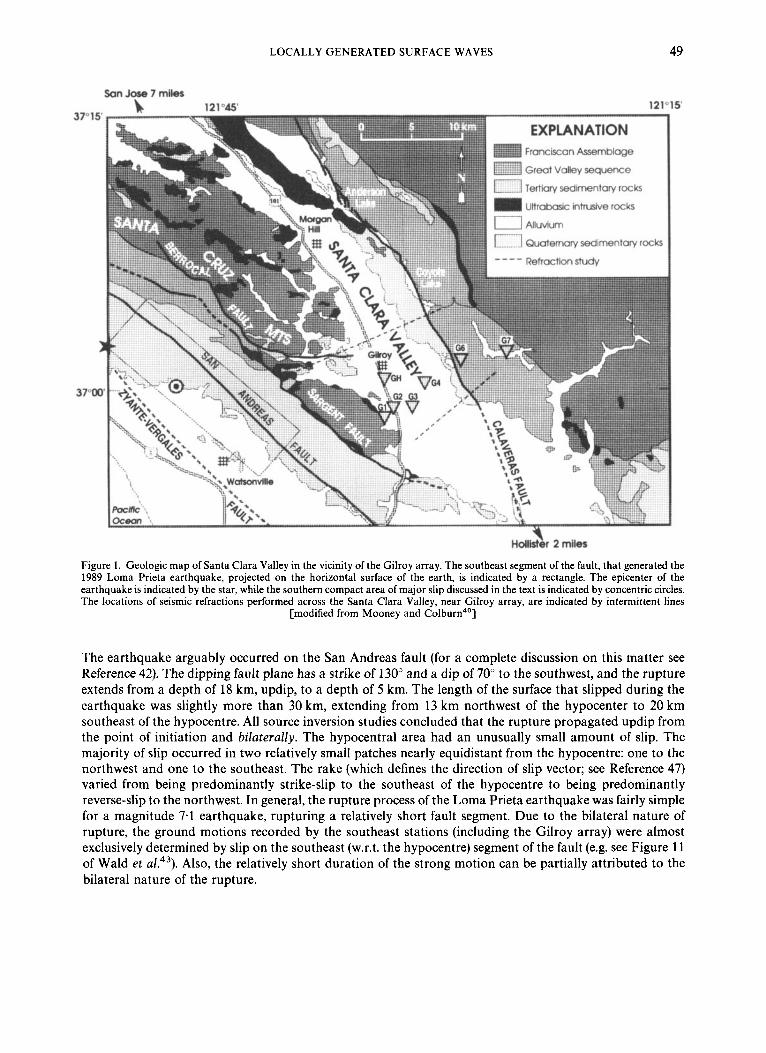
The response (particle velocities) of the Santa Clara Valley to the Lorna Prieta earthquake, as recorded by the Gilroy array is shown in Figure 2(a). The two horizontal orthogonal components of motion have been rotated so as to be oriented along the radial and transverse (i.e. tangential) directions with respect to the localized area of large slip on the fault plane (indicated in Figure 1 by concentric circles). Trigger times are available for the recorded data3' and the records have been aligned accordingly on a common time axis. Stations G1, G2, G3 and G4 are located at equal intervals along a line connecting stations G1 and G7 (Figure 1). Stations G1 and G6 are sited on rock, while stations G2, G3 and G4 are located on alluvium. Visual inspection of the velocity time histories in Figure 2(a) shows that the traces recorded at G2, G3 and G4 are more complex, and have longer duration and higher amplitudes than the traces recorded at G1 and G6. This is clearly evident by comparing the vertical components of particle motion which suggest the presence of Rayleigh waves propagating across the valley. Figure 2(b), which shows the same data bandpass filtered

LOM

A P

RIE

TA 1

989:

Dis

plac

emen

t tFm

inS.

3, F

max

=l.2

] SV

wav

e D

ispl

acem

ent:

azi=

-30

inc=

30 F

cS.6

Hz Q=50

G1-

G2 1

-B

G1

%

._

. -

._

_..

.. .

-I

-

-*-

1 1

1 I

Rad

ial-V

ertic

al C

ompo

nent

s R

adia

l-Ver

tical

Com

pone

nts

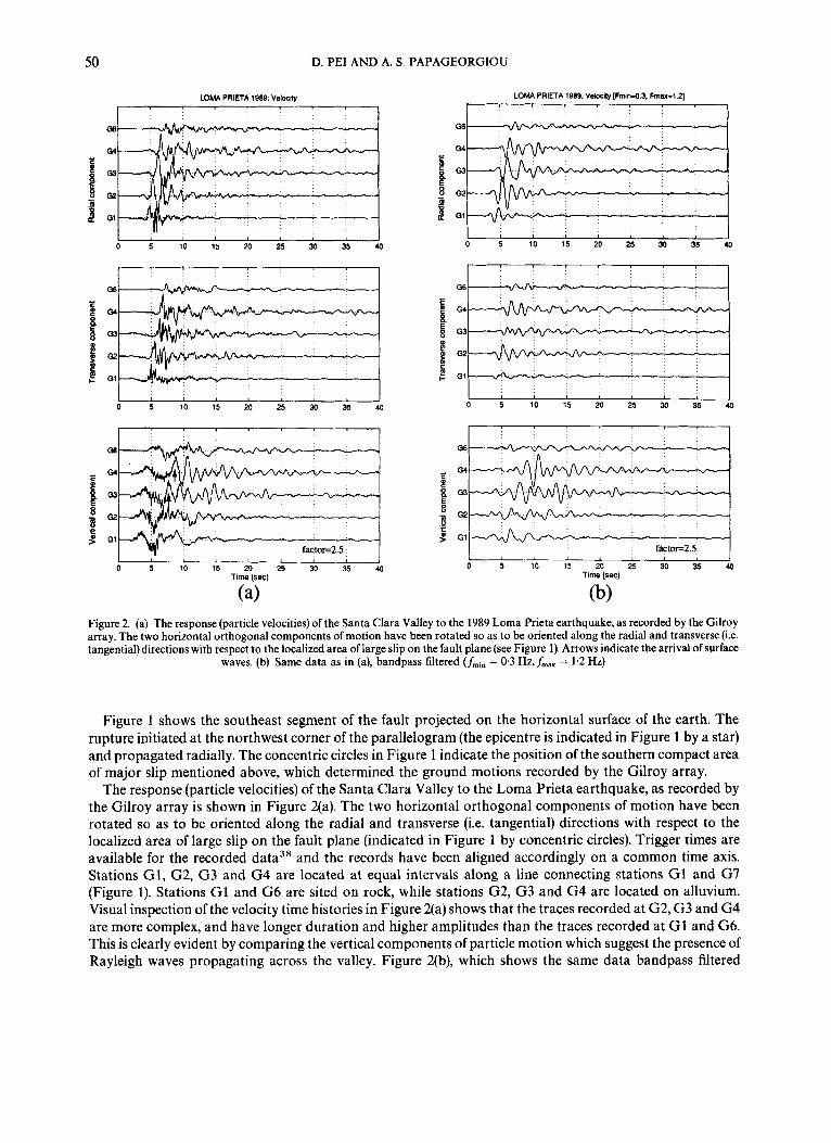
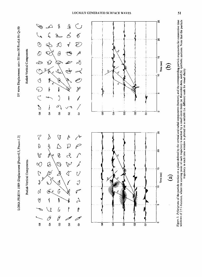
Figu

re 3

. Po

larig

rarn

s of t

he p

artic

le m

otio

n on

a p

lane

def

ined

by

the

verti

cal a

nd ra

dial

com

pone

nts

(bot

tom

), an

d th

e co

rres

pond

ing

parti

cle

traj

ecto

ries

for c

onse

cutiv

e tim

e w

indo

ws

of 2

.5 s

dura

tion,

whe

re th

e st

artin

g po

int

of e

ach

traje

ctor

y is

mar

ked

by a

sm

all c

ircle

(top

). (a

) R

ecor

ded

data

, and

(b)

synt

hetic

mot

ions

. Not

e th

at th

e pa

rticl

e tra

ject

ory

in e

ach

time

win

dow

is p

lotte

d on

a s

uita

ble

(i.e.

diff

eren

t) sc

ale

for v

isua

l cla

rity


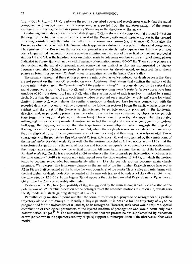
(fmin = 0.3 Hz,fm,, = 1.2 Hz), reinforces the picture described above, and reveals more clearly that the radial component is dominant over the transverse one, as expected from the radiation pattern of the source mechanism (i.e. the source radiates primarily SV-waves in the direction of the array).

Continuing our analysis of the recorded data (Figure 2(a)), on the vertical component (at around 2 4 s from the origin of the time axis) we notice the arrival of the P-wave, with initial particle motion in the upward direction, consistent with the radiation pattern of the source mechanism (e.g. Reference 47). Soon after the P-wave we observe the arrival of the S-wave which appears as a distinct strong pulse on the radial component. The signature of the P-wave on the vertical component is a relatively high-frequency oscillation which rides over a longer period harmonic. Focusing now our attention on the traces of the vertical component recorded at stations G3 and G4, as the high-frequency oscillation starts to fade away we observe the arrival of strong phases (indicated in Figure 2(a) with arrow) with frequency of oscillation around 0.6-0.7 Hz. These strong phases are also evident on the radial component, albeit somewhat less distinct as they are accompanied by higher- frequency oscillations (which are probably scattered S-waves). As already noted, we interpret these strong phases as being valley-induced Rayleigh waves propagating across the Santa Clara Valley.

The primary reason that these strong phases are interpreted as valley-induced Rayleigh waves is that they are not present on the trace G1 recorded on rock. Additional illustrations that confirm the validity of the above interpretation are (i) the “polarigrams” of the particle motion4* on a plane defined by the vertical and radial components (bottom, Figure 3(a)), and (ii) the corresponding particle trajectories for consecutive time windows of 2.5 s duration (top, Figure 3(a)), where the starting point of each trajectory is marked by a small circle. Note that the trajectory in each time window is plotted on a suitable (i.e. different) scale for visual clarity. [Figure 3(b), which shows the synthetic motions, is displayed here for easy comparison with the recorded data, even though it will be discussed in the following section.] From the particle trajectories it is evident that the onset of the S-waves is characterized by particle motions polarized in the horizontal direction and, in particular, primarily in the radial direction (as was confirmed by checking the particle trajectories on a horizontal plane, not shown here). This is reassuring in that it suggests that the rotated orthogonal horizontal components of motion are in fact the radial and transverse components of motion. Following the S-waves, we notice that the trajectories become elliptical, which suggests the arrival of Rayleigh waves. Focusing on stations G 3 and G4, where the Rayleigh waves are well developed, we notice that the elliptical trajectories are prograde (i.e. clockwise rotation) and their major axis is horizontal. This is characteristic of thefirst higher Rayleigh model R , (e.g. Reference 49), and as suggested by the simulations, of the second higher Rayleigh mode R2 as well. On the motion recorded at G3 we notice at t = 13.5 s that the trajectories change abruptly the sense of rotation and become retrograde (i.e. counterclockwise rotation) and their major axis approaches now the vertical direction. All these features signal the arrival of the fundamental Rayleigh mode R, . On the trace recorded at G4 we observe that the prograde particle motion which starts in the time window 7.5-10 s is temporarily interrupted over the time window 12.5-15 s, in which the motion tends to become retrograde, but immediately after t = 15 s the particle motion becomes again clearly prograde. We interpret this temporary change as the arrival of the first higher Rayleigh mode (marked as RT in Figure 3(a)) generated at the far side (i.e. east boundary) of the Santa Clara Valley and interfering with the first higher Rayleigh mode R,-generated at the near side (i.e. west boundary) of the valley at G4-over the time window 12-5-15 s. From Figure 3(a), it appears that the fundamental Rayleigh mode R , arrives at G4 at time t - 20 s, considerably attenuated.

Evidence of the R 1 phase (and possibly of R Z , as suggested by the simulations) is clearly visible also on the polarigrams of G2. Careful inspection of the polarigrams of the recorded motions at station G2, reveals also the Ro mode as it starts gaining strength at t = 7.5 s.

Parenthetically we should point out that the sense of rotation (i.e. prograde or retrograde) of a particle trajectory alone is not enough to identify a Rayleigh mode. It is possible for the trajectory of Ro to be prograde and for the trajectories of R 1 and R z to be retrograde. However, such cases would require a special combination of rheological parameters of the layered medium of propagation and would occur only over narrow period The numerical simulations that we present below, supplemented by dispersion curves (not shown in the paper for economy of space) support our interpretation of the observed surface wave modes.


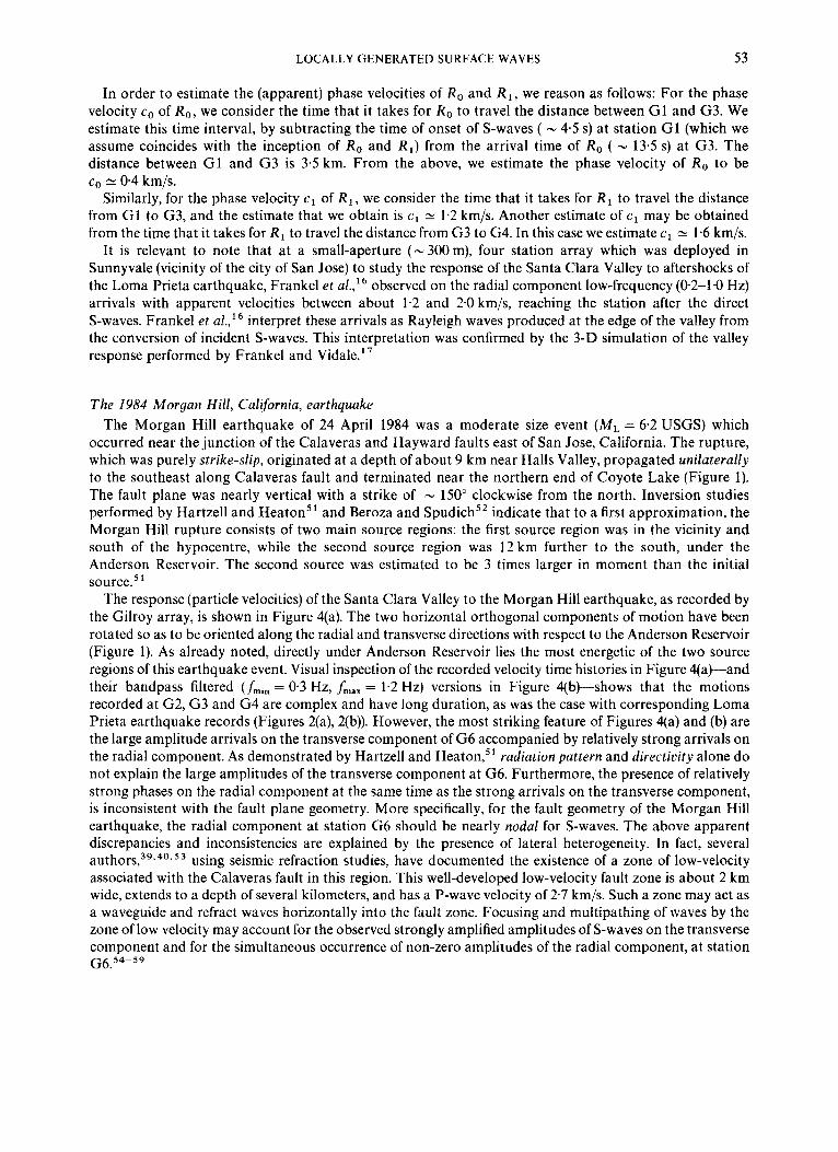
In order to estimate the (apparent) phase velocities of Ro and R t , we reason as follows: For the phase velocity co of Ro, we consider the time that it takes for KO to travel the distance between G1 and G3. We estimate this time interval, by subtracting the time of onset of S-waves ( - 4-5 s) at station G1 (which we assume coincides with the inception of Ro and R,) from the arrival time of Ro ( - 13.5 s) at G3. The distance between G1 and G3 is 3 5 km. From the above, we estimate the phase velocity of Ro to be co N 0.4 km/s.

Similarly, for the phase velocity c1 of R1, we consider the time that it takes for R1 to travel the distance from G1 to G3, and the estimate that we obtain is c, N 1.2 km/s. Another estimate of c1 may be obtained from the time that it takes for R1 to travel the distance from G3 to G4. In this case we estimate c1 1: 1.6 km/s.

It is relevant to note that at a small-aperture ( N 300 m), four station array which was deployed in Sunnyvale (vicinity of the city of San Jose) to study the response of the Santa Clara Valley to aftershocks of the Loma Prieta earthquake, Frankel et a1.,16 observed on the radial component low-frequency (0.2-1.0 Hz) arrivals with apparent velocities between about 1.2 and 2.0 km/s, reaching the station after the direct S-waves. Frankel et a1.,16 interpret these arrivals as Rayleigh waves produced at the edge of the valley from the conversion of incident S-waves. This interpretation was confirmed by the 3-D simulation of the valley response performed by Frankel and Vidale.I7

The 1984 Morgan Hill, California, earthquake The Morgan Hill earthquake of 24 April 1984 was a moderate size event ( M L = 6.2 USGS) which

occurred near the junction of the Calaveras and Hayward faults east of San Jose, California. The rupture, which was purely strike-slip, originated at a depth of about 9 km near Halls Valley, propagated unilaterally to the southeast along Calaveras fault and terminated near the northern end of Coyote Lake (Figure 1). The fault plane was nearly vertical with a strike of - 150” clockwise from the north. Inversion studies performed by Hartzell and Heaton’l and Beroza and SpudichS2 indicate that to a first approximation, the Morgan Hill rupture consists of two main source regions: the first source region was in the vicinity and south of the hypocentre, while the second source region was 12 km further to the south, under the Anderson Reservoir. The second source was estimated to be 3 times larger in moment than the initial source.’

The response (particle velocities) of the Santa Clara Valley to the Morgan Hill earthquake, as recorded by the Gilroy array, is shown in Figure 4(a). The two horizontal orthogonal components of motion have been rotated so as to be oriented along the radial and transverse directions with respect to the Anderson Reservoir (Figure 1). As already noted, directly under Anderson Reservoir lies the most energetic of the two source regions of this earthquake event. Visual inspection of the recorded velocity time histories in Figure 4(a)-and their bandpass filtered (fmin = 0.3 Hz, fm,, = 1.2 Hz) versions in Figure 4(b)-shows that the motions recorded at G2, G3 and G4 are complex and have long duration, as was the case with corresponding Loma Prieta earthquake records (Figures 2(a), 2(b)). However, the most striking feature of Figures 4(a) and (b) are the large amplitude arrivals on the transverse component of G6 accompanied by relatively strong arrivals on the radial component. As demonstrated by Hartzell and Heaton,’l radiation pattern and directivity alone do not explain the large amplitudes of the transverse component at G6. Furthermore, the presence of relatively strong phases on the radial component at the same time as the strong arrivals on the transverse component, is inconsistent with the fault plane geometry. More specifically, for the fault geometry of the Morgan Hill earthquake, the radial component at station G6 should be nearly nodal for S-waves. The above apparent discrepancies and inconsistencies are explained by the presence of lateral heterogeneity. In fact, several a ~ t h o r s , ~ ~ , ~ ~ , ’ ~ using seismic refraction studies, have documented the existence of a zone of low-velocity associated with the Calaveras fault in this region. This well-developed low-velocity fault zone is about 2 km wide, extends to a depth of several kilometers, and has a P-wave velocity of 2.7 km/s. Such a zone may act as a waveguide and refract waves horizontally into the fault zone. Focusing and multipathing of waves by the zone of low velocity may account for the observed strongly amplified amplitudes of S-waves on the transverse component and for the simultaneous occurrence of non-zero amplitudes of the radial component, at station (36.54-59


0 6

G4

EE G4

B - 8

i

MI-

"a EE

GZ-

G1-

I

8 G I

E G 4 t 8 " 8 G Z 1 f 0 1

0 5 10 15 20 25 30 35 40 Time (sec)

m 5 $ 0 2

2 G1

G 2 g

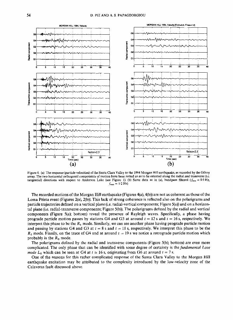
Figure 4. (a) The response (particle velocities) of the Santa Clara Valley to the 1984 Morgan Hill earthquake, as recorded by the Gilroy array. The two horizontal orthogonal components of motion have been rotted so as to be oriented along the radial and transverse (i.e. tangential) directions with respect to Anderson Lake (see Figure 1). (b) Same data as in (a), bandpass filtered (fmin = 0.3 Hz,

fma. = 1.2 Hz)

1 5

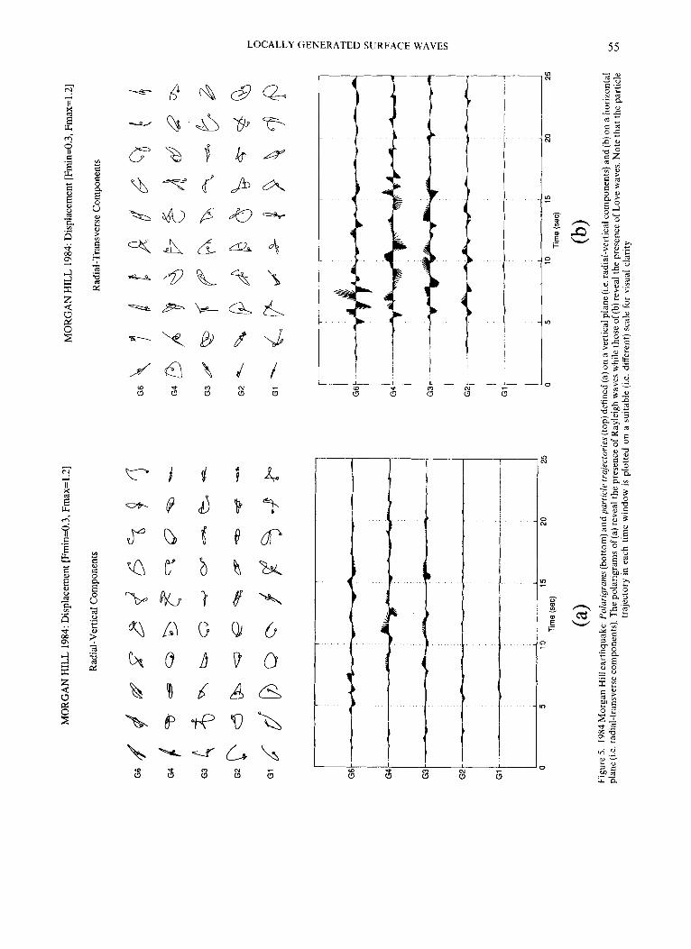
The recorded motions of the Morgan Hill earthquake (Figures 4(a), qb)) are not as coherent as those of the Loma Prieta event (Figures 2(a), 2(b)). This lack of strong coherence is reflected also on the polarigrams and particle trajectories defined on a vertical plane (i.e. radial-vertical components; Figure 5(a)) and on a horizontal plane (i.e. radial-transverse components; Figure 5(b)). The polarigrams defined by the radial and vertical components (Figure 5(a); bottom) reveal the presence of Rayleigh waves. Specifically, a phase having prograde particle motion passes by stations G4 and G3 at around t = 12 s and t = 16 s, respectively. We interpret this phase to be the R1 mode. Similarly, we can see another phase having prograde particle motion and passing by stations G4 and G3 at t = 8 s and t = 11 s, respectively. We interpret this phase to be the R2 mode. Finally, on the trace of G4 and at around t = 19 s we notice a retrograde particle motion which probably is the Ro mode.

The polarigrams defined by the radial and transverse components (Figure 5(b); bottom) are even more complicated. The only phase that can be identified with some degree of certainty is the fundamental Love mode Lo which can be seen at G4 at t N 16 s, originating from G6 at around t = 7 s.

One of the reasons for this rather complicated response of the Santa Clara Valley to the Morgan Hill earthquake excitation may be attributed to the complexity introduced by the low-velocity zone of the Calaveras fault discussed above.

G2-

GI- - facto~2.5

56 D. PEI AND A. S . PAPAGEORGIOU

Y

Figure 6 . The valley model used to perform the numerical simulations. The model is two-dimensional, having an infinitely long axis. The seismic excitation may consist of plane body or surface waves, approaching the valley from any azimuthal direction rp with any

incidence angle i . Even though the valley model is 2-D, the response is 3-D

SIMULATION O F THE VALLEY RESPONSE

In order to reinforce our interpretation of the data presented above, we have performed numerical simulations of the Santa Clara Valley response to seismic excitation. The model used to perform the numerical simulations is shown in Figure 6.32,28 The valley model is two-dimensional, having an infinitely long axis. The seismic excitation may consist of plane body or surface waves, approaching the valley from any azimuthal direction cp with any incidence angle i. Even though the valley model is two-dimensional, the response is three-dimensional. We believe, that such a model is adequate to study, at least qualitatively, important aspects of the earthquake response of the Santa Clara Valley in the vicinity of the Gilroy array. We state at the outset that the simulations are not aimed at reproducing exactly the waveforms of the recorded motions. Rather, we attempt to reproduce the valley-induced surface waves, expecting that the type of surface-wave modes and their apparent phase velocities along the array can be simulated adequately with a relatively simple model, like the one we use in this study.

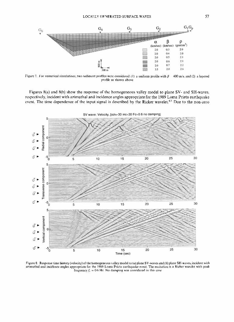
The overall shape of the cross-section of the valley (i.e. the sediment-rock interface) is reasonably well-known from the refraction studies of Mooney and L ~ e t g e r t ~ ~ and Mooney and C ~ l b u r n . ~ ' At each station of the Gilroy array, holes were drilled to a depth of 30 to 60 m and the S- and P-wave velocity were measured.60-61 Since none of these holes reached the depth to bedrock, an additional hole was drilled at station G2 to a depth of 197 m, and Franciscan rock was encountered at the base of the alluvium at 180 m. Station G2 is underlain by 13 m of Holocene alluvium, 8 m of late Pleistocene alluvium and 18 m of Pleistocene lacustrine deposits overlying poorly sorted alluvium of the Santa Clara f ~ r m a t i o n . ~ ~ , ~ ~ We do not have any information about the S-wave velocities of the deeper strata of the valley (i.e. deeper than - 200 m). Frankel and Vidale" used a value of S-wave velocity, /3 = 600 m/s, in their analysis of the Santa Clara Valley earthquake response in the vicinity of San Jose. For our numerical simulations we consider two, rather idealized, sediment profiles: (1) a uniform profile with fl = 400 m/s, and (2) a layered profile as shown in Figure 7. The layering in the latter profile is not based on any actual data, but it has been selected because it is physically plausible. Given the limited data that are available to us, we thought that the above two profiles should be adequate in capturing, at least in a qualitative sense, any important aspects of the long period response of the valley.


2 1 2.0 0.5 2 0 0 6 2 1

2.0 0 7 2 2 500 rn Eg 3 5 2.0 2 6

Figure 7. For numerical simulations, two sediment profiles were considered: (1) a uniform profile with p = 400 mjs, and (2) a layered profile as shown above

Figures 8(a) and 8(b) show the response of the homogeneous valley model to plane SV- and SH-waves, respectively, incident with azimuthal and incidence angles appropriate for the 1989 Loma Prieta earthquake event. The time dependence of the input signal is described by the Ricker wavelet.62 Due to the non-zero

SV wave: Velocity, [azi=-30 inc=30 Fc=0.6 no damping]

-0 5 10 15 20 25 30

5

0

-5 .-- . v

0 5 10 15 20 25 30

5 10 15 Time (sec)

20 25 30

Figure 8. Response time history (velocity) of the homogeneous valley model to (a) plane SV-waves and (b) plane SH-waves, incident with azimuthal and incidence angles appropriate for the 1989 Loma Prieta earthquake event. The excitation is a Ricker wavelet with peak

frequencyf, = 0.6 Hz. No damping was considered in this case


SH wave: Velocity, [azi=-30 inc=30 Fc=0.6 no damping]

5

d

C W

3 , " 0

-5 0 5 10 15 20 25 30

Time (sec)

Figure 8(b)

azimuthal angle (9 = - 30"), the response of the sediments is three-dimensional, i.e. the out-of-plane motions of the two-dimensional cross-section of the valley are coupled with the in-plane-motions, and thus the incident plane waves induce both Rayleigh and Love wave modes. The dominant features of the response in both cases are the fundamental and first higher Rayleigh modes R , and R1, respectively, and the fundamental Love mode Lo. As expected, for the case of incident SV-wave (Figure 8(a)) the direct arrival is evident in the radial component and excites strongly the Ro and R 1 modes, while for the case of incident SH-waves (Figure 8(b)), the direct arrival is evident in the transverse component and excites strongly the Lo mode. As we have already pointed out, the incident wave on the Gilroy array for the Lorna Prieta event is primarily a SV-wave. The simulations shown in Figures 8(a) and 8(b) were made assuming zero damping (i.e. quulityfuctor Q = co) and this explains the strong reflected phases originating from the eastern side (i.e. far side) of the valley.

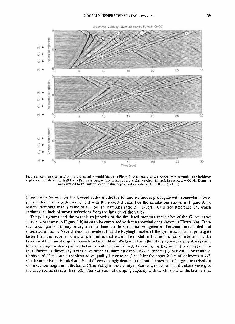
Figure 9 shows the response of the layered valley model to an incident plane SV-wave. Comparing the response of the layered valley model (Figure 9) with the response of the homogeneous valley model (Figure 8(a)) we see several common features (e.g. excitation of the R,, R , , and Lo modes), but we also observe two rather obvious differences. First, in the response of the layered valley model (Figure 9) we notice the appearance of the second higher Rayleigh mode R2 which is clearly evident in the radial component. The R, mode is absent, or at least not clearly evident, in the response of the homogeneous valley model


SV wave: Velocity, [aZi=-30 inc=30 Fc=0.6 Q=50]

Time (sec)

Figure 9. Response (velocity) of the layered valley model (shown in Figure 7) to plane SV-waves incident with azimuthal and incidence angles appropriate for the 1989 Loma Prieta earthquake. The excitation is a Ricker wavelet with peak frequencyf, = 0.6 Hz. Damping

was assumed to be uniform for the entire deposit with a value of Q = 50 (k ( = 0.01)

(Figure 8(a)). Second, for the layered valley model the Ro and R1 modes propagate with somewhat slower phase velocities, in better agreement with the recorded data. For the simulations shown in Figure 9, we assume damping with a value of Q = 50 (i.e. damping ratio 5 = 1/(2Q) = 0.01) (see Reference 17), which explains the lack of strong reflections from the far side of the valley.

The polarigrams and the particle trajectories of the simulated motions at the sites of the Gilroy array stations are shown in Figure 3(b) so as to be compared with the recorded ones shown in Figure 3(a). From such a comparison it may be argued that there is at least qualitative agreement between the recorded and simulated motions. Nevertheless, it is evident that the Rayleigh modes of the synthetic motions propagate faster than the recorded ones, which implies that either the model in Figure 6 is too simple or that the layering of the model (Figure 7) needs to be modified. We favour the latter of the above two possible reasons for explaining the discrepancies between synthetic and recorded motions. Furthermore, it is almost certain that different sedimentary layers have different damping capacities (i.e. different Q values). [For instance, Gibbs et ~ l . , ~ ~ measured the shear-wave quality factor to be Q N 12 for the upper 200 m of sediments at G2. On the other hand, Frankel and Vidale" convincingly demonstrate that the presence of large, late arrivals in observed seismograms in the Santa Clara Valley in the vicinity of San Jose, indicates that the shear wave Q of the deep sediments is at least 50.1 This variation of damping capacity with depth is one of the factors that


SH wave: Velocity, [azi=-120 inc=45 Fc=0.6 Q=50]

Time (sec)

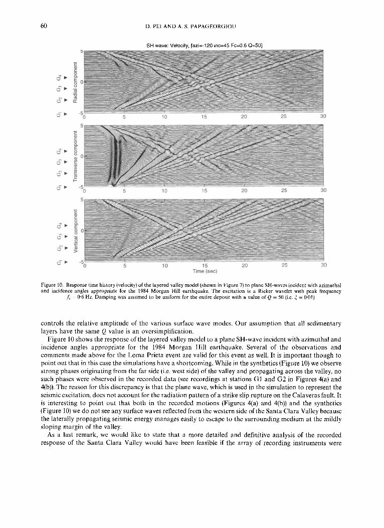
Figure 10. Response time history (velocity) of the layered valley model (shown in Figure 7) to plane SH-waves incident with azimuthal and incidence angles appropriate for the 1984 Morgan Hill earthquake. The excitation is a Ricker wavelet with peak frequency

fc = 0.6 Hz. Damping was assumed to be uniform for the entire deposit with a value of Q = 50 (i.e. 5 = 0.01)

controls the relative amplitude of the various surface wave modes. Our assumption that all sedimentary layers have the same Q value is an oversimplification.

Figure 10 shows the response of the layered valley model to a plane SH-wave incident with azimuthal and incidence angles appropriate for the 1984 Morgan Hill earthquake. Several of the observations and comments made above for the Loma Prieta event are valid for this event as well. It is important though to point out that in this case the simulations have a shortcoming. While in the synthetics (Figure 10) we observe strong phases originating from the far side (i.e. west side) of the valley and propagating across the valley, no such phases were observed in the recorded data (see recordings at stations G1 and G2 in Figures 4(a) and 4(b)). The reason for this discrepancy is that the plane wave, which is used in the simulation to represent the seismic excitation, does not account for the radiation pattern of a strike slip rupture on the Calaveras fault. It is interesting to point out that both in the recorded motions (Figures 4(a) and 4(b)) and the synthetics (Figure 10) we do not see any surface waves reflected from the western side of the Santa Clara Valley because the laterally propagating seismic energy manages easily to escape to the surrounding medium at the mildly sloping margin of the valley.

As a last remark, we would like to state that a more detailed and definitive analysis of the recorded response of the Santa Clara Valley would have been feasible if the array of recording instruments were


considerably denser and two-dimensional instead of sparse and linear, as the existing array. In such a case, it would have been possible to infer the phase velocity and direction of propagation of all surface wave modes-and thus identify the location of their origin/generation along the boundary of the valley-on a more firm basis (e.g. References 64 and 23). However, given the limitations of the existing sparse linear array at Gilroy, we believe that with our analysis we have succeeded in demonstrating evidence of valley-induced surface waves and in extracting from the data their most important features.

CONCLUSION

We have presented an analysis of the motions of the 1989 Loma Prieta and 1984 Morgan Hill earthquakes as recorded by the linear Gilroy array which runs across the Santa Clara Valley, and we have attempted to simulate important features of the recorded motions using a relatively simple model. The aforementioned two earthquake events originated on the San Andreas and Calaveras faults, respectively, which bound on opposite sides and run parallel to the axis of the Santa Clara Valley. The motivation for this study is to present additional observational evidence of valley-induced surface waves, and to investigate potential variations of the azimuthal direction of the incoming seismic excitation. Our task was complicated parti- cularly by the presence of the low velocity zone of the Calaveras fault, which traps and focuses seismic energy generated by slip on the fault, and leaks it to the surrounding medium in a rather complicated manner.

According to our analysis, both earthquakes events excite strongly several surface wave modes (Ro, R , , Rz, L o ) inside the Santa Clara Valley. These surface waves are valley-induced since they are not present on the rock site of the array at the edge of the valley closest to the source. They are produced by conversion of incident S-waves at the edges of the valley and propagate across it.

The synthetic motions generated by the simulations, reproduce important aspects of the valley response, such as surface wave types and phase velocities. A better quantitative agreement of the synthetics with the recorded data would require a better control of the sediment properties (i.e. wave velocities, attenuation factors and thickness of the sedimentary layers) and a more realistic representation of the seismic sources than the plane wave assumption that we used in our modelling technique.

ACKNOWLEDGMENTS

This research was supported by U.S. Geological Survey Grant 1434-92-G-2168, and by Contract No. NCEER 93-2001 under the auspices of the National Center for Earthquake Engineering Research under NSF Grant No. ECE-86-07591. The research was conducted using the Cornell National Supercomputer Facility (CNSF), a resource of the Center for Theory and Simulations in Science and Engineering (Cornell Theory Center), which receives major funding from the National Science Foundation and IBM Corporation, with additional support from New York State and members of the Corporate Research Institute.

REFERENCES

1. K. Aki and K. L. Larner, ‘Surface motion of a layered medium having an irregular interface due to incident plane SH-waves’, J .

2. D. M. Boore, K. L. Larner and K. Aki, ‘Comparison of two independent methods for the solution of wave-scattering problems:

3. M. D. Trifunac, ‘Surface motion of a semi-cylindrical alluvial valley for incident plane SH-waves’, Bull. seism. soc. Am. 61, 1755-~1770

4. J . Lysmer and L. A. Drake, ‘A finite element method for seismology’, in B. A. Bolt (ed.), Methods ofCornputational Physics, Vol. 11,

5. L. A. Drake and A. K. Mal, ‘Love and Rayleigh waves in the San Fernando Valley’, Bull. seism. soc. Amer. 62, 1673--1690 (1972). 6. T. L. Hong and D. V. Helmberger. ‘Glorified optics and wave propagation is nonplanar structures’, Bull. seism. soc. Amer. 68,

7. P.-Y. Bard and M. Bouchon, ‘The seismic response of sediment-filled valleys. Part I. The case of incident SH waves’, Bull. seism. soc.

8. P.-Y. Bard and M. Bouchon, ‘The seismic response of sediment-filled valleys. Part 11. The case of incident P and SV waves’, Bull.

9. P.-Y. Bard and M. Bouchon, ‘The two-dimensional resonance of sediment-filled valleys’, Bull. seism. SOC. Am. 75, 519-541 (1985).

geophys. res. IS, 933- 954 (1970).

response of a sedimentary basin to vertically incident SH-waves’, J . yeophys. res. 76, 558-569 (1971).

(1971).

Academic Press, New York, 1972, pp.181-216.

131 3-1 330 (1978).

Am. 70, 1263-1286 (1980).

seism. SOC. Am. 70, 1921-1941 (1980).


10. J. L. King and B. E. Tucker, ‘Observed variation of earthquake motion across a sediment-filled valley’, Bull. seism. soc. Am. 74,

11. J. E. Vidale and D. V. Helmberger, ‘Elastic finite-difference modeling of the 1971 San Fernando California earthquake’, Bull. seism. soc. Am. 78, 122-141 (1988).

12. H. Kawase and K. Aki, ‘A study on the response of a soft basin for incident S, P, and Rayleigh waves with special reference to the long duration observed in Mexico city’, Bull. seism. soc. Amer. 79, 1361-1382 (1989).

13. F. J. Sanchez-Sesma, L. E. Perez-Rocha and S. Chavez-Perez, ‘Diffraction of elastic waves by three-dimensional surface irregulari- ties. Part II’, Bull. seism. soc. Amer. 79, 101- 112 (1989).

14. T. K. Mossessian and M. Dravinski, ‘Amplification of elastic waves by three dimensional valley. Part 11: Transient response’, Earthquake eng. struct. dyn. 19, 681491 (1990).

15. A. S. Papageorgiou and J. Kim, ‘Study of the propagation and amplification of seismic waves in Caracas Valley with reference to the July 29, 1967 earthquake: SH-waves’, Bull. seism. soc. Am. 81, 2214-2233 (1991).

16. A. Frankel, S. Hough, P. Friberg and R. Busby, ‘Observations of Loma Prieta aftershocks from a dense array in Sunnyvale, California’, Bull. seism. soc. Am. 81, 1900- 1922 (1991).

17. A. Frankel and J. E. Vidale, ‘A three-dimensional simulation of seismic waves in the Santa Clara Valley, California from a Loma Prieta aftershock’, Bull. seism. soc. Am. 82, 204-2074 (1992).

18. S. Phillips, S. Kinoshita and H. Fujiwara, ‘Basin-induced Love waves observed using the strong motion array at Fuchu, Japan’, Bull. seism. soc. Am. 83, 64-84 (1993).

19. R. W. Graves, ‘Modeling three-dimensional site response effects in the Marina District Basin, San Francisco, California’, Bull. seism. soc. Am. 83, 1042-1063 (1993).

20. K. Yomogida and J. T. Etgen, ‘3-D wave propagation in the Los Angeles basin for the Whittier-Narrows earthquake’, Bull. seism. soc. Am. 83, 1325-1344 (1993).

21. Y. Hisada, K. Aki and T.-L. Teng, ‘3-D simulations of surface wave propagation in the Kanto sedimentary basin, Japan. Part 2: application of the surface wave BEM’, Bull. seism. soc. Am. 83, 1700-1720 (1993).

22. A. Frankel, ‘Three-dimensional simulations of ground motions in the San Bernardino Valley, California, for hypothetical earthquakes on the San Andreas Fault’, Bull. seism. soc. Am. 83, 1020-1041 (1993).

23. A. Frankel, ‘Dense array recordings in the San Bernardino Valley of Landers-Big Bear aftershocks: basin surface waves, Moho reflections, and three-dimensional simulations’, Bull. seism. soc. Am. 84, 613-624 (1994).

24. F. J. Sanchez-Sesma, J. Ramos-Martinez and M. Campillo, ‘An indirect boundary element method applied to simulate the seismic response of alluvial valleys for incident P, S and Rayleigh waves’, Earthquake eng. struct. dyn. 22, 279-295 (1993).

25. A. Ohtsuki and K. Harumi, ‘Effect of topography and subsurface inhomogeneities on seismic SV waves’, Earthquake eng. struct. dyn. 11, 441462 (1983).

26. A. Ohtsuki, H. Yamahara and T. Tazoh, ‘Effect of lateral inhomogeneity on seismic waves, 11: observations and analyses’, Earthquake eng. struct. dyn. 12, 795-816 (1984).

27. P. Spudich and M. Iida, ‘The seismic coda, site effects, and scattering in alluvial basins studied using aftershocks of the 1986 North Palm Springs, California, earthquake as source arrays’, Bull. seism. soc. Am. 83, 1721-1743 (1993).

28. B. Zhang, A. S. Papageorgiou and J. L. Tassoulas, ‘A hybrid numerical technique, combining the finite element and boundary element methods for modeling elastodynamic scattering problems’, Proc. lUth ASCE eng. mech. specialty con$. Boulder, Colorado, May 21-24, 1995, in press.

29. K. R. Khair, S. K. Datta and A. H. Shah, ‘Amplification of obliquely incident seismic waves by cylindrical alluvial valleys of arbitrary cross-sectional shape. Part I. Incident P and SV waves’, Bull. seism. soc. Am. 79, 610-630 (1989).

30. J. E. Luco, H. L. Wong and F. C. P. De Barros, ‘Three-dimensional response of a cylindrical canyon in a layered half-space’, Earthquake eng. struct. dyn. 19, 799-817 (1990).

31. L. Zhang and A. K. Chopra, ‘Three-dimensional analysis of spatially varying ground motion around a uniform canyon in a homogeneous half-space’, Earthquake eng. struct. dyn. 20, 91 1-926 (1991).

32. D. Pei and A. S. Papageorgiou, ‘Study of the response of cylindrical alluvial valleys of arbitrary cross-section to obliquely incident seismic waves using the discrete wavenumber boundary element method’, Sixth inr. conf: soil dynamics and earthquake eng., Bath, U.K., June 14-16, 1993, pp. 149-161.

33. H. Pedersen, F. J. Sanchez-Sesma and M. Campillo, ‘Three-dimensional scattering by two-dimensional topographies’, Bull. seism. soc. Am. 84, 1169-1183 (1994).

34. J. E. Luco and F. C. P. de Barros, ‘Three-dimensional response of a layered cylindrical valley embedded in a layered half-space’, Earthquake eng. struct. dyn. 24, 109-125 (1995).

35. D. Jongmans and M. Campillo, ‘The response of the Ubaye Valley (France) for incident SH and SV waves: comparison between measurements and modeling’, Bull. seism. soc. Am. 83,907-924 (1993).

36. A. G. Brady, P. N. Mork, V. Perez and L. D. Poter, ‘Processed data from the Gilroy array and Coyote Creek records, Coyote Lake, California Earthquake 6 August, 1979’, U.S. Geological Survey Open-Fole Report 81-42, 1981, 171p.

37. A. F. Shakal, M. J. Huang, D. L. Parke and R. W. Sherburne, ‘Processed data from the strong-motion records of the Morgan Hill earthquake of 24 April 1984. Part I : ground-response records’, California Strong Motion Insrrumentation Program, Report No. OSMS 85-04, 1986, 249p.

38. A. Shakal, M. J. Huang, M. Reichle, C. Ventura, T. Cao, R. W. Sherburne, M. Savage, R. Darragh and C. Petersen, ‘CSMIP strong-motion records from the Santa Cruz Mountains (Loma Prieta), California earthquake of 17, October 1989’, California Strong Motion Instrumentation Program Report No. OSMS 89-06, 1989, 195p.

39. W. D. Mooney and J. H. Leutgert, ‘A seismic refraction study of the Santa Clara Valley and the southern Santa Cruz mountains, west-central California’, Bull. seism. soc. Am. 72, 901-909 (1982).

40. W. D. Mooney and R. H. Colburn, ‘A seismic-refraction profile across the San Andreas, Sargent and Calaveras Faults, west-central California’, Bull. seism. soc. Am. 75, 175-191 (1985).

137-151 (1984).


41. W. B. Joyner, R. E. Warrick and T. E. Fumal, ‘The effect of quaternary alluvium on strong ground motion in the Coyote Lake,

42. G. C. Beroza, ‘Near-source modeling of the Loma Prieta earthquake: evidence for heterogeneous slip and implications for

43. D. J. Wald, D. V. Helmberger and T. H. Heaton, ‘Rupture model of the 1989 Loma Prieta earthquake from the inversion of

44. J. H. Steidl, R. J. Archuleta and S. H. Hartzell, ‘Rupture history of the 1989 Loma Prieta, California earthquake’, Bull. seism. soc. Am.

45. S. H. Hartzell, G. S. Stewart and C. Mendoza, ‘Comparison of L1 and L, norms in a teleseismic inversion for the slip history of the

46. Y. Zeng, ‘Deterministic and stochastic modeling of the high frequency seismic wave generation and propagation in the lithosphere’,

47. K. Aki and P. G. Richards, ‘Quantitative Seismology: Theory and Methods’, W. H. Freeman and Co., New York, 1980. 48. P. Bernard and A. Zollo, ‘Inversion of near-source S polarization for parameters of double-couple point sources’, Bull. seism. soc.

49. H. M. Mooney and B. A. Bolt, ‘Dispersive characteristics of the first three Rayleigh modes for a single surface layer’, Bull. seism. soc.

50. K. E. Bullen and B. A. Bolt, An Introduction to the Theory ?/Seismology, 4th edn., Cambridge University Press, Cambridge, 1985. 51. S. H. Hartzell and T. H. Heaton, ‘Rupture history of the 1984 Morgan Hill California earthquake from the inversion of strong

motion records’, Bull. seism. soc. Am. 76, 649474 (1986). 52. G. C . Beroza and P. Spudich, ‘Linearized inversion for fault rupture behavior: application to the 1984 Morgan Hill, California

earthquake’, J . geophys. res. 93, 62756296 (1988). 53. P. Blumling, W. D. Mooney and W. H. K. Lee, ‘Crustal structure of the southern Calaveras fault zone, central California, from

seismic refraction investigations’, Bull. seism. soc. Am. 75, 193-209 (1985). 54. R. Feng and T. V. McEvilly, ‘Interpretation of seismic reflection profiling data for the structure of the San Andreas Fault zone’, Bull.

seism. soc. Am. 73, 1701-1720 (1983). 55. V. F. Cormier and P. Spudich, ‘Amplification of ground motion and waveform complexity in fault zones: examples from the San

Andreas and Calaveras faults’, Geophys. j. roy. astron. soc. 79, 135-152 (1984). 56. V. F. Cormier and G. C. Beroza, ‘Calculation of strong ground motion due to an extended earthquake source in a laterally varying

structure’, Bull. seism. soc. Am. 77, 1Ll3 (1987). 57. Y.-G. Li, P. C. Leary, K. Aki and P. E. Malin, ‘Seismic trapped modes in the Oroville and San Andteas fault zones’, Science 249,

763-766 (1990). 58. Y.-G. Li, K. Aki, D. Adams, A. Hasemi and W. H. K. Lee, ‘Seismic guided waves trapped in the zone of the Landers, California,

earthquake of 1997, J. geophys. res. 99, 11 705-1 1 722 (1994). 59. V. F. Cormier and W.-J. Su, ‘Effects of three-dimensional crustal structure on the estimated slip history and ground motion of the

Loma Prieta earthquake’, Bull. seism. soc. Am. 84, 284-294 (1994). 60. T. E. Fumal, ‘A compilation of the geology and measured and estimated shear-wave velocity profiles at strong-motion stations that

recorded the Loma Prieta, California, earthquake’, U.S. Geological Survey, Open-File Report 91-31!, 1991. 61. J. F. Gibbs, T. E. Fumal, D. M. Boore and W. B. Joyner, ‘Seismic velocities and geologic logs from borehole measurements a t seven

strong-motion stations that recorded the Loma Prieta earthquake’, U.S. Geological Survey Open-File Report, Y2-287, 1992, 139p. 62. N. Ricker, ‘The computation of output disturbances from amplifiers for true wavelet inputs’, Geophysics 10, 207-220 (1945). 63. J. F. Gibbs, D. M. Boore, W. B. Joyner and T. E. Fumal, ‘The attenuation of seismic shear waves in quaternary alluvium in Santa

64. N. A. A brahamson and B. A. Bolt, ‘Array analysis and synthesis mapping of strong seismic motion, in B. A. Bolt (ed.), Seismic Strong

California earthquake of 1979’, Bull. seism. soc. Am. 71, 1333-1349 (1981).

earthquake hazard’, Bull. seism. soc. Am. 81, 1603-1621 (1991).

strong-motion and broadband teleseismic data’, Bull. seism. soc. Am. 81, 154C1572 (1 991).

81, 1573-1602 (1991).

Loma Prieta, California earthquake’, Bull. seism. soc. Am. 81, 1518-1539 (1991).

Ph.D. Thesis, University of Southern California, Los Angeles, California, 1991.

Am. 79, 1779-1809 (1989).

Am. 56, 43--67 ( 1 966).

Clara Valley, California’, Bull. seism. soc. Am. 84, 76 -90 (1994).

Motion Synthetics’, Academic Press, New York, 1987.

locally generated surface waves in santa clara valley: analysis of observations and numerical...

Documents