LETTERSPUBLISHED ONLINE: 14 AUGUST 2011 | DOI: 10.1038/NGEO1219

Locally enhanced precipitation organized byplanetary-scale waves on TitanJonathan L. Mitchell1*, Máté Ádámkovics2, Rodrigo Caballero3,4 and Elizabeth P. Turtle5

Saturn’s moon Titan exhibits an active weather cycle thatinvolves methane1–8. Equatorial and mid-latitude clouds canbe organized into fascinating morphologies on scales exceed-ing 1,000 km (ref. 9). Observations include an arrow-shapedequatorial cloud that produced detectable surface accumula-tion, probably from the precipitation of liquid methane10. Ananalysis of an earlier cloud outburst indicated an interplaybetween high- and low-latitude cloud activity, mediated byplanetary-scale atmospheric waves11. Here we present a com-bined analysis of cloud observations and simulations with athree-dimensional general circulation model of Titan’s atmo-sphere, to obtain a physical interpretation of observed storms,their relation to atmosphere dynamics and their aggregateeffect on surface erosion. We find that planetary-scale Kelvinwaves arise naturally in our simulations, and robustly orga-nize convection into chevron-shaped storms at the equatorduring the equinoctial season. A second and much slowerwave mode organizes convection into southern-hemispherestreaks oriented in a northwest–southeast direction, similarto observations9. As a result of the phasing of these modes,precipitation rates can be as high as twenty times the localaverage in our simulations. We conclude that these events,which produce up to several centimetres of precipitation overlength scales exceeding 1,000 km, play a crucial role in fluvialerosion of Titan’s surface.

Titan’s slow rotation (16 terrestrial days) and small radius (40%that of Earth) conspire to allow a global Hadley circulation, thetropical meridional overturning circulation of the atmosphere.As a result, Titan’s strongest zonal winds are shifted polewardsrelative to Earth’s, meridional temperature gradients are weak12,and baroclinic cyclogenesis associated with storm-track weatheris suppressed13. This dynamical configuration gives Titan an ‘alltropics’ climate14. Titan’s intertropical convergence zone (ITCZ)migrates fromone summer hemisphere to the other.Models predicta transient phase just following equinoxes when the ITCZ passesover the equator14–16 and, during this time, Earth-like tropicaldisturbances would be expected at Titan’s equator9,17.

Classical shallow-water theory18 predicts the existence of a broadspectrum of linear equatorial wave modes, including equatorially-trapped Rossby, Kelvin and mixed Rossby-gravity waves. All ofthese modes can be detected in Earth’s atmosphere throughspectral analysis of observations, which show power concentratedat planetary scales (>104 km; ref. 19). Through their surfaceconvergence and induced vertical motion, the modes collectivelyorganize the location and timing of clouds and precipitationin Earth’s tropics on intraseasonal timescales. As a result oflow insolation and a stabilizing antigreenhouse effect20, moist

1Earth & Space Sciences, Atmospheric & Oceanic Sciences, University of California, Los Angeles, California 90095, USA, 2Astronomy Department,University of California, Berkeley, California 94720, USA, 3Department of Meteorology (MISU), Stockholm University, 106 91 Stockholm, Sweden,4Bert Bolin Centre for Climate Research, Stockholm University, 106 91 Stockholm, Sweden, 5Johns Hopkins University, Applied Physics Laboratory, Laurel,Maryland 20723, USA. *e-mail: jonmitch@ucla.edu.

convection on Titan cannot be maintained purely through surfaceevaporative fluxes, indicating that moisture convergence providedby large-scale modes of circulation is important for convectivecloud formation14,16,17,21,22.

Titan’s methane clouds have received much attention sincethey were first discovered spectroscopically1. Although cloud-coveris spatially limited, large outbursts of cloud activity occasionallyoccur23, as do cloud-free conditions24.Mesoscale clouds can remainstationary for days22,25,26. Titan’s seasons progress slowly, takingroughly seven years to transition from solstice to equinox. Themostrecent northern spring equinox (NSE) occurred on 11 August 2009.Since that time, the location of cloud activity has shifted from south-ern (summer)mid- andhigh-latitudes to the equatorial region9,26,27.

More recently, Cassini Imaging Science Subsystem (ISS) imagesof Titan have revealed large-scale clouds with an interesting arrayof morphologies and characteristics9. Most strikingly, an arrow-shaped cloud oriented eastwards was observed at the equator on27 September 2010 (ref. 9), followed by observations of surfacewetting which gradually diminished over several months10.We nowuse our fully three-dimensional Titan general circulation model(GCM) (described in Methods and Supplementary Information)to examine the dynamical origin of these storms, and wedevelop a methodology for comparing model precipitation rates tocloud observations.

Cloud opacity depends on the sizes and amount of suspended,condensed methane. Our Titan GCM has a moist convectionscheme which predicts a surface precipitation rate, and weassume precipitation is associated with optically thick clouds. Asmall number of physically motivated assumptions (described inMethods and Supplementary Information) allow us to simulatecloud opacity in ISS bands using the GCM’s precipitation field,thereby quantitatively linking cloud opacity to the amount ofprecipitation. Simulated observations of two events during theequinoctial transition of our GCM are shown in Fig. 1b,e. Thetwo cloud events observed by Cassini ISS are shown in Fig. 1c,f:a cloud shaped like a chevron at the equator pointing eastwardswas observed on 27 September 2010, followed on 18 October 2010by a streak of clouds extending southeastwards from low-latitudesto high-latitudes9. Figure 1 demonstrates that our Titan GCMproduces convective storms with the basic morphology of the twocloud observations. The dynamics underlying these storms are nowexamined through diagnostics of the GCM.

Figure 2 shows snapshots of the GCM simulation of Titanshortly following NSE. During this time, the ITCZ is passing overthe equator and establishing itself in the northern hemisphere(Supplementary Fig. S7). Figure 2a,c shows the surface windfield with the zonal mean subtracted (arrows) and the 15-day

NATURE GEOSCIENCE | VOL 4 | SEPTEMBER 2011 | www.nature.com/naturegeoscience 589© 2011 Macmillan Publishers Limited. All rights reserved.

LETTERS NATURE GEOSCIENCE DOI: 10.1038/NGEO1219

a b c

d e f

Figure 1 | Titan’s clouds (right) are organized by planetary-scale waves that dominate storm activity in model simulations (centre). a,d, Simulations ofcloud-free observations at 938 nm with lines of latitude and longitude used for comparison with models that include cloud opacity distributions (b,e) setby the precipitation from the GCM output as described in Methods (shown in Fig. 2). Viewing geometry and illumination angle are selected to reproduceCassini observations9 on 27 September 2010 (c) and 18 October 2010 (f). GCMmodels (b,e) are divided by a simulated 619 nm image to reproduce theimage processing used for the observations. No parameter tuning is required to produce a similar contrast to observations, indicating a closecorrespondence between the modelled precipitation field and the observed clouds.

Latit

ude

Longitude

Chevron

360° 270° W 180° W 90° W 0°

Longitude

60° S

30° S

0°

30° N

60° N

Longitude

Fast-eastward wave

Longitude

Streak Slow-westward wave

0

0.4

0.8

1.2

1.6

2.0

(cm)

0

0.4

0.8

1.2

1.6

2.0

a

c

b

d

Latit

ude

60° S

30° S

0°

30° N

60° N

Latit

ude

60° S

30° S

0°

30° N

60° N

Latit

ude

60° S

30° S

0°

30° N

60° N

(cm)

360° 270° W 180° W 90° W 0° 360° 270° W 180° W 90° W 0°

360° 270° W 180° W 90° W 0°

Figure 2 | Simulated precipitation and surface wind patterns in selected events during the equinoctial season (left column) and derived from statisticalanalysis (right column). a, Fifteen-terrestrial-day cumulative precipitation (blue, cm) and surface winds with the zonal mean subtracted (arrows) for anequatorial chevron-shaped event. b, Regression of the leading principal component associated with eastward-propagating variance (see SupplementaryInformation) onto the surface winds (arrows) and precipitation (colours). c, As in a but for a mid-latitude streak event. The length of wind vector arrowshave been increased by a factor of three. d, As in b but for westward-propagating variance.

cumulative precipitation of the events shown in Fig. 1b,e (blue, cm).The cumulative precipitation of these storms indicates greatlyenhanced precipitation rates compared with the global- andtime-mean of less than 0.1mmd−1. Near the equator, zonallyelongated bands of precipitation are being maintained by thecirculation, marking the location of the ITCZ. Figure 2a clearlyshows a chevron precipitation feature at longitude 260◦ W at the

equator that is spatially coincident with a region of horizontalconvergence of surface winds, indicating a role for gravity waves.The chevron produces one to two centimetres of precipitation overa 2,000-km-wide region during its lifetime, an amount sufficientto create runoff and erosion of the equatorial surface28. A fewmonths of integration later, the model produces a precipitation andwind pattern extending from the equator deep into the southern

590 NATURE GEOSCIENCE | VOL 4 | SEPTEMBER 2011 | www.nature.com/naturegeoscience© 2011 Macmillan Publishers Limited. All rights reserved.

NATURE GEOSCIENCE DOI: 10.1038/NGEO1219 LETTERShemisphere, as seen in Fig. 2c. This streaking precipitation isproduced by a combination of convergent and circulating surfacewinds, indicating a role for both gravity waves and Rossby waves.The depth of convection in the streaking feature is shallowerthan the chevron (Supplementary Fig. S6), however its lifetime isconsiderably longer, resulting in several centimetres of precipitationover its extent. Currently published ISS images do not showevidence for surface changes associated with the storm in Fig. 1f,which suggests these clouds do not produce substantial rainfall. Thisindicates that our model overestimates the amount of mid-latitudeprecipitation during the current season.

Precipitation rates within these modes exceed the zonal- andtime-mean rate by a factor of∼20 during the equinoctial transition(Fig. 3a).We infer that three-dimensional dynamics are responsiblefor local and significant enhancements in precipitation, and aretherefore essential for understanding the observed distribution ofsurface erosion29. Equatorial chevrons are ephemeral features ofTitan’s climate, however, occurring on the order of an Earth yearas Titan’s ITCZ undergoes a post-equinoctial transition from onehemisphere to the other (Supplementary Figs S7 and S10; ref. 17).Surface accumulation (that does not infiltrate into the regolith)evaporates away during the summer (Supplementary Fig. S8), withimportant implications for observed fluvial features in Titan’ssemi-arid environment29.

We now show that the cloud structures in the examples aboveare not isolated occurrences, but instead constitute the ‘typical’behaviour of convection in the model, organized by well-defineddynamical modes of the atmosphere. The evolution in time andlongitude of modelled equatorial precipitation (Fig. 3a) showsevidence of eastward-propagating disturbances with a phase speedof about 12m s−1 (indicated by the solid black line), superposedon slower disturbances travelling westwards at around 1m s−1

(dashed line). These two modes of variability are also apparentin a space–time power spectrum of equatorial surface zonal wind(Fig. 3b), which shows sharp peaks at an eastward-propagatingzonal wavenumber of 2 with a period of about eight days(corresponding to a phase speed of about 12m s−1 at the equator)and at a westward-propagating zonal wavenumber of 2 with period∼ 100 days (phase speed ∼ 1m s−1). This close correspondencebetween precipitation and surface wind perturbations implies alink between dynamical and convective processes, as seen inconvectively coupled equatorial waves on Earth19.

To isolate the spatial structure of the dominant eastward andwestward modes, we follow a three-step procedure described inMethods. The spatial structure and phase speed of the eastward-propagating mode corresponds closely to that of a baroclinic,equatorially trappedKelvinwave (see Supplementary Information).The spatial patterns of precipitation and surface wind anomaly ofthis mode are shown in Fig. 2c. Crucially, these waves are associatedwith roughly chevron-shaped equatorial precipitation patterns. Thewestward-propagatingmode (Fig. 2d) stretches from the equator tothe high-latitudes of the Southern Hemisphere, and is associatedwith a streak-like precipitation feature stretching southeastwardsfrom the tropics into the mid-latitudes. Thus, convective storms inthe GCM are organized by large-scale modes of variability, and themodes are robustly associated in a statistical sensewith precipitationstructures resembling the observed clouds.

We have also conducted sensitivity tests to investigate thefeedback of moist convective heating onto the dynamical modes(see Supplementary Information for details). In a simulation wherelatent heating by convection and surface evaporation is artificiallysuppressed, we find that the eastward-propagating Kelvin modeis unchanged, whereas the westward mode is substantially altered(Fig. 3c). Thus the Kelvin mode is convectively uncoupled (seeSupplementary Information), although its surface convergence fieldplays an important role in organizing precipitation. Convection

0

50

100

150

200

Tim

e (d

ays)

Perio

d (d

ays)

Longitude

¬4 ¬2 0 2 4

100

40

20

10

8

Perio

d (d

ays)

100

40

20

10

8

Zonal wavenumber

¬4 ¬2 0 2 4Zonal wavenumber

0

5

10

15

20a

b

c

360° 270° W 180° W 90° W 0°

Figure 3 | Space–time variability of simulated equatorial winds andprecipitation averaged over ±10◦ latitude in the Titan GCM.a, Longitude–time distribution of precipitation rate normalized to theglobal- and time-mean rate for the period containing the chevron event inFig. 1 (magenta triangle at day 30) and the streak event (triangle at day210). Lines indicate constant velocity trajectories of 11.7ms−1 eastwards(solid) and 0.9ms−1 westwards (dashed). b, Space–time spectraldecomposition of surface zonal winds for 1,000 simulation days centredaround the equinox. c, As in b but for a test simulation with the latentheating of methane removed.

is essential to the dynamics of the westward mode, however, asindicated by the substantial reduction of precipitation at negativewavenumbers in the test case (Fig. 3c; also see SupplementaryInformation). This is the first evidence of a convectively coupledwave on a planetary body other than Earth.

A sequence of cloud observations taken in 2008 (before NSE)with ground-based instruments indicated a connection betweendisturbances at equatorial and polar latitudes likely to be mediatedby planetary-scale waves11. This cloud propagated eastwards at∼3m s−1, and was interpreted as a stationary Rossby waveadvected by the mid-tropospheric wind. However, our simulationindicates that the eastward-propagating precipitation field duringthis epoch is associated with the Kelvin wave component. As thisobservation occurred before NSE, surface convergence resulting

NATURE GEOSCIENCE | VOL 4 | SEPTEMBER 2011 | www.nature.com/naturegeoscience 591© 2011 Macmillan Publishers Limited. All rights reserved.

LETTERS NATURE GEOSCIENCE DOI: 10.1038/NGEO1219

from the superposition of the Kelvin mode and the ITCZ is mostintense south of the equator (Supplementary Fig. S10). As theseason transitions towards Northern Summer Solstice (NSS), ourmodel indicates a shift in the precipitation by the Kelvin–ITCZsuperposition to northern mid-latitudes accompanied by southernmid-latitude streaks.We therefore predict a phase of transient cloudactivity in both hemispheres of Titan during the next several years(Supplementary Fig. S7).

In summary, we have developed a process for interpretingthe morphologies of and precipitation associated with Titan’sclouds through a combined analysis of observations and GCMsimulations, thereby opening a new field of dynamic meteorology.We find that recent cloud activity near Titan’s equator justfollowing NSE is consistent with the presence of two dominantmodes of atmospheric variability in the GCM. A fast, eastward-propagating mode travelling at ∼12m s−1 with the character ofan equatorially trapped Kelvin wave produces chevron-shapedprecipitation patterns similar to the clouds observed by CassiniISS on 27 September 2010 (ref. 9). A slow, westward-propagatingmode that is vertically confined accounts for streaks of precipitationsuch as the cloud observed on 18 October 2010 (ref. 9). Thislatter mode is convectively coupled, the first of its kind to beinferred outside of Earth’s atmosphere. The phasing of thesemodes produce several centimetres of precipitation over 1,000-km-scale regions, locally enhancing precipitation rates by 20-foldover the mean. These modes therefore play a crucial role influvial erosion of Titan’s surface. Observations clearly indicatesurface changes associated with the equatorial chevron10, butprecipitation from themid-latitude streak is too light to be detected,indicating the model overestimates mid-latitude precipitationduring the current season.

MethodsOur Titan GCM is similar to that used in a previous study16, the primary differencebeing that the model is now fully three-dimensional. Simplified treatments ofradiation, convection, and the seasonal cycle are included. The model does notinclude tides, either thermal (diurnal) or gravitational (semi-diurnal), nor anyother non-axisymmetric forcing mechanism (be it topography, albedo, opacitysources, or others.). The atmosphere is spun up and moistened by methaneevaporation from an initial state of solid-body rotation and zero methanehumidity. The seasonal cycle of insolation is included in the model forcing; seethe Supplementary Information for a more detailed description. A (statistical)steady state is achieved after ∼20 Titan years (∼600 Earth years). The resultsshown in the figures are from 1,000 terrestrial days bracketing NSE of the 21stsimulated Titan year. (The zonal- and time-mean overturning streamfunction,zonal winds, and temperature of the full, 1,800 model days are shown in theSupplementary Information.)

The GCM does not include a cloud scheme, so we have developed a methodfor simulating cloud observations based on precipitation. Briefly, we assume clouddroplets are distributed about a peak size of 512 µm, which are marginally loftedfor convective updrafts of 10m s−1, typical for deep convective events on Titan21.We assume 10–20% of the column precipitation remains suspended, with acloud-top altitude of 20 km. Together the columnmass of the cloud and the dropletsize distribution determine the cloud optical depth. Mie theory then translatesthe droplet size distribution into the scattering properties of clouds, ultimatelylinking the precipitation field from the GCM to the radiative transfer model (seeSupplementary Information for more details).

To isolate the spatial structure of dominant modes of variability in theGCM, the surface zonal wind field is spectrally filtered to retain only the spaceand timescales of the dominant spectral peaks; the leading patterns of variabilityof the filtered surface wind are extracted using empirical orthogonal function(EOF) analysis, and the associated three-dimensional fields are reconstructed byregression onto the leading principal component; further details are given in theSupplementary Information.

Received 5 April 2011; accepted 1 July 2011; published online14 August 2011

References1. Griffith, C., Owen, T., Miller, G. & Geballe, T. Transient clouds in Titan’s lower

atmosphere. Nature 395, 575–578 (1998).

2. Griffith, C., Hall, J. & Geballe, T. Detection of daily clouds on Titan. Science290, 509–513 (2000).

3. Tokano, T. et al. Methane drizzle on Titan. Nature 442, 432–435 (2006).4. Ádámkovics, M., Wong, M., Laver, C. & de Pater, I. Widespread morning

drizzle on Titan. Science 318, 962–965 (2007).5. Brown, M., Smith, A., Chen, C. & Ádámkovics, M. Discovery of fog at the

south pole of Titan. Astrophys. J. Lett. 706, L110–L113 (2009).6. Turtle, E. et al. Cassini imaging of Titan’s high-latitude lakes, clouds, and

south-polar surface changes. Geophys. Res. Lett. 36, L02204 (2009).7. Turtle, E., Perry, J., Hayes, A. & McEwen, A. Shoreline retreat at Titan’s

Ontario Lacus and Arrakis Planitia from Cassini Imaging Science Subsystemobservations. Icarus 212, 957–959 (2011).

8. Hayes, A. G. et al. Transient surface liquid in Titan’s polar regions fromCassini.Icarus 211, 655–671 (2011).

9. Turtle, E. et al. Seasonal changes in Titan’s meteorology. Geophys. Res. Lett. 38,L03203 (2011).

10. Turtle, E. et al. Rapid and extensive surface changes near Titan’s equator:Evidence of April showers. Science 331, 1414–1417 (2011).

11. Schaller, E., Roe, H., Schneider, T. & Brown, M. Storms in the tropics of Titan.Nature 460, 873–875 (2009).

12. Achterberg, R., Conrath, B., Gierasch, P., Flasar, F. & Nixon, C. Titan’smiddle-atmospheric temperatures and dynamics observed by the CassiniComposite Infrared Spectrometer. Icarus 194, 263–277 (2008).

13. Mitchell, J. & Vallis, G. The transition to superrotation in terrestrialatmospheres. J. Geophys. Res. 115, E12008 (2010).

14. Mitchell, J., Pierrehumbert, R., Frierson, D. & Caballero, R. Thedynamics behind Titan’s methane clouds. Proc. Natl Acad. Sci. USA 103,18421–18426 (2006).

15. Tokano, T. Impact of seas/lakes on polar meteorology of Titan: Simulation bya coupled GCM-Sea model. Icarus 204, 619–636 (2009).

16. Mitchell, J., Pierrehumbert, R., Frierson, D. & Caballero, R. The impact ofmethane thermodynamics on seasonal convection and circulation in a modelTitan atmosphere. Icarus 203, 250–264 (2009).

17. Mitchell, J. The drying of Titan’s dunes: Titan’s methane hydrology and itsimpact on atmospheric circulation. J. Geophys. Res. 113, E08015 (2008).

18. Matsuno, T. Quasi-geostrophic motions in the equatorial area. J. Meteor. Soc.Jpn 44, 25–42 (1966).

19. Wheeler, M. & Kiladis, G. Convectively coupled equatorial waves: Analysis ofclouds and temperature in the wavenumber–frequency domain. J. Atmos. Sci.56, 374–399 (1999).

20. McKay, C., Pollack, J. & Courtin, R. The greenhouse and antigreenhouse effectson Titan. Science 253, 1118–1121 (1991).

21. Barth, E. L. & Rafkin, S. C. R Convective cloud heights as a diagnostic formethane environment on Titan. Icarus 206, 467–484 (2010).

22. Ádámkovics, M., Barnes, J., Hartung, M. & de Pater, I. Observations of astationary mid-latitude cloud system on Titan. Icarus 208, 868–877 (2010).

23. Schaller, E., Brown, M., Roe, H. & Bouchez, A. A large cloud outburst at Titan’ssouth pole. Icarus 182, 224–229 (2006).

24. Schaller, E., Brown, M., Roe, H., Bouchez, A. & Trujillo, C. Dissipation ofTitan’s south polar clouds. Icarus 184, 517–523 (2006).

25. Roe, H., Brown, M., Schaller, E., Bouchez, A. & Trujillo, C. Geographic controlof Titan’s mid-latitude clouds. Science 310, 477–479 (2005).

26. Rodriguez, S. et al. Global circulation as the main source of cloud activity onTitan. Nature 459, 678–682 (2009).

27. Brown, M., Roberts, J. & Schaller, E. Clouds on Titan during the Cassini primemission: A complete analysis of the VIMS data. Icarus 205, 571–580 (2010).

28. Jaumann, R. et al. Fluvial erosion and post-erosional processes on Titan. Icarus197, 526–538 (2008).

29. Langhans,M. et al. Titan’s fluvial valleys:Morphology, distribution, and spectralproperties. Planet. Space Sci. http://dx.doi.org/10.1016/j.pss.2011.01.020(in the press).

AcknowledgementsE.P.T. is supported by NASA’s Cassini–Huygens mission.

Author contributionsJ.L.M. contributed experiment design, performed GCM simulation analysis, and wrotethe manuscript. M.Á. and J.L.M. developed the algorithm for simulating clouds from theGCM, and M.Á. contributed radiative transfer analysis of the GCM. R.C. contributedthe statistical analysis of the GCM simulation and J.L.M. and R.C. interpreted the modeldynamics. E.P.T. contributed analysis of Cassini ISS cloud images.

Additional informationThe authors declare no competing financial interests. Supplementary informationaccompanies this paper on www.nature.com/naturegeoscience. Reprints and permissionsinformation is available online at http://www.nature.com/reprints. Correspondence andrequests for materials should be addressed to J.L.M.

592 NATURE GEOSCIENCE | VOL 4 | SEPTEMBER 2011 | www.nature.com/naturegeoscience© 2011 Macmillan Publishers Limited. All rights reserved.

SUPPLEMENTARY INFORMATIONDOI: 10.1038/NGEO1219

NATURE GEOSCIENCE | www.nature.com/naturegeoscience 1

Supplementary Information for: Locally enhancedprecipitation organized by planetary-scale waves on Titan

Jonathan L. Mitchell,1∗ Mate Adamkovics,2

Rodrigo Caballero,3,4 Elizabeth P. Turtle5

1Earth & Space Sciences, Atmospheric & Oceanic SciencesUniversity of California, Los Angeles, CA 90095, USA

2Astronomy Department, University of California, Berkeley, CA 94720, USA3Department of Meteorology (MISU), Stockholm University, Stockholm, Sweden

4Bert Bolin Center for Climate Research, Stockholm University, Stockholm, Sweden5Johns Hopkins University, Applied Physics Laboratory, Laurel, MD 20723, USA

1 Method for producing simulated cloud observations fromGCM precipitation

Radiative TransferImages of Titan’s clouds have been interpreted as regions of moist convection and used to

study circulation in the lower atmosphere. We describe a methodology for using the output fromthe circulation models described here to predict cloud morphologies. The simulated images arecompared with observations from Cassini/ISS at a wavelength, λ=938 nm.Base model

The atmospheric temperature, pressure, and composition are setup according to our previousradiative transfer model ([1] and references therein). This model has been used to study cloudmorphologies and spectra[2]. The difference here is that we use the most recently reported methanegas opacities[3] and adopt the aerosol scattering properties and vertical (altitude) opacity structureused to interpret measurements made by the Huygens probe[4]. We fit 0.935µm phase functions[4]with high order Legendre polynomials (Figure S1), and use the discrete ordinates method (DISORT)with 48 streams to solve the radiative transfer. A Cassini/ISS map (http://ciclops.org, PIA11149)of the surface at 938nm is used as an input for the surface reflectivity, stretched between values of1 – 25%, consistent with the ∼16% reflectivity measured at the Huygens landing site. Similarly,a 619nm image is calculated using the aerosol scattering phase function reported at 600nm. Thiswavelength is insensitive to the surface or atmosphere below 100km and is used for simulation ofthe Cassini/ISS image processing[5].Cloud Scattering

We calculate the scattering properties of a cloud that is defined by a distribution of spherical

1

Locally enhanced precipitation organized by planetary-scale waves on Titan

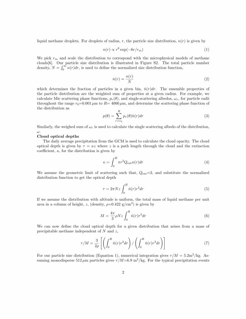
liquid methane droplets. For droplets of radius, r, the particle size distribution, n(r) is given by

n(r) ∝ r6 exp(−6r/rm) (1)

We pick rm and scale the distribution to correspond with the microphysical models of methaneclouds[6]. Our particle size distribution is illustrated in Figure S2. The total particle numberdensity, N =

�∞0 n(r)dr, is used to define the normalized size distribution function,

n(r) =n(r)N

(2)

which determines the fraction of particles in a given bin, n(r)dr. The ensemble properties ofthe particle distribution are the weighted sum of properties at a given radius. For example, wecalculate Mie scattering phase functions, pr(θ), and single-scattering albedos, ωr, for particle radiithroughout the range r0=0.001µm to R= 4000µm, and determine the scattering phase function ofthe distribution as

p(θ) =R�

r=r0

pr(θ)n(r)dr (3)

Similarly, the weighed sum of ωr is used to calculate the single scattering albedo of the distribution,ω.Cloud optical depths

The daily average precipitation from the GCM is used to calculate the cloud opacity. The cloudoptical depth is given by τ = κz where z is a path length through the cloud and the extinctioncoefficient, κ, for the distribution is given by

κ =� R

0πr

2Qextn(r)dr (4)

We assume the geometric limit of scattering such that, Qext=2, and substitute the normalizeddistribution function to get the optical depth

τ = 2πNz

� R

0n(r)r2

dr (5)

If we assume the distribution with altitude is uniform, the total mass of liquid methane per unitarea in a column of height, z, (density, ρ=0.422 g/cm3) is given by

M =4π

3ρNz

� R

0n(r)r3

dr (6)

We can now define the cloud optical depth for a given distribution that arises from a mass ofprecipitable methane independent of N and z,

τ/M =32ρ

��� R

0n(r)r2

dr

�/

�� R

0n(r)r3

dr

��(7)

For our particle size distribution (Equation 1), numerical integration gives τ/M = 5.2m2/kg. As-

suming monodisperse 512µm particles gives τ/M=6.9 m2/kg. For the typical precipitation events

2

scattering angle [deg]

phas

e fun

ctio

n

50.0 100.0 150.00.1

1.0

10.0

100.0 935nm600nm

Figure S1: Aerosol scattering phase functions at 600nm and 935nm reported by [4]. Scatteringat 935 nm reported for regions above and below 80 km (black squares and triangles, respectively).Aerosol scattering at 600nm, used to simulate Cassini/ISS image processing in [5], is sensitive to theatmosphere above 100km, and a single phase function is reported (grey squares). The best fit 64thand 48th order Legendre polynomials (solid lines) are used to fit the phase functions at 600nm and935nm. High order polynomials are required to fit the strongly forward-scattering phase functions.

shown in Figures 1 and 2 of the main text (e.g., the chevron feature) the precipitation rate of1.2×10−5 kg/m2/s equates to M ∼ 1 kg/m2 when integrated over the GCM timestep of 1 day.If ∼10–20% of the precipitable moisture is in cloud droplets (consistent with terrestrial clouds),then the chevron feature from the precipitation field in the GCM results in an optically thick cloudfeature in the simulated observations.Clouds of frozen methane

[7] used a steady-state condensation model with the Voyager temperature profile to predict thatclouds would be composed of liquid droplets below ∼12 km and solid crystals above. The shapeof the crystals could be octahedral or cubic, as suggested for solar system ices in general by [8].The vapor-pressure of methane measured by the Huygen’s probe was used to calculate the relativehumidity of methane over mixed methane-nitrogen cloud droplets and solid methane cloud particlesby [9]. These results suggested a ‘sub-visible’ liquid methane-nitrogen cloud below ∼16 km and acloud of solid methane extending from 20–40 km.

The time-dependent cloud microphysical model of [6] considered the condensation of methaneonto ethane coated hydrocarbon aerosol (haze) particles. This followed their earlier work on theheterogenous nucleation of ethane onto aerosol particles and ethane cloud formation [10]. In theirmodel, methane nucleates onto an ethane cloud particle creating an ice crystal, which serves asthe condensation nucleus for addition methane or ethane creating ‘mixed’ clouds. The crystalsare significantly smaller than the methane droplets. Our particle size distribution, with a peak at

3

1 10 100 1000radius [µm]

10-10

10-8

10-6

10-4

10-2

dN/d

(log

r) [

cm-3

]

Figure S2: A cloud particle size distribution with rm=512µm is broadly consistent with methaneclouds at 10–20 km predicted by Barth & Toon, 2006.

0 50 100 150 scattering angle, [deg]

-3

-2

-1

0

1

2

3

phas

e fu

nctio

n, lo

g p

() rm = 512 !m

Figure S3: Cloud scattering phase function at λ=938 nm for a distribution of spherical droplets(solid curve), and the best fit 48th order Legendre polynomial (squares). Optical constants forliquid methane, nr=1.288 and ni= 1.1×10−6. The value for ni has been linearly interpolatedbetween data reported at 888.5 nm and 974.2 nm. The single scattering albedo, ω, for the cloud is∼1 since 4πnirm/λ� 1.

4

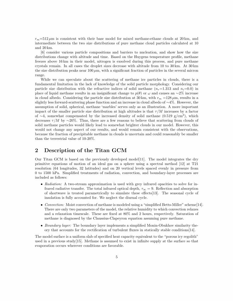
rm=512µm is consistent with their base model for mixed methane-ethane clouds at 20 km, andintermediate between the two size distributions of pure methane cloud particles calculated at 10and 20 km.

[6] consider various particle compositions and barriers to nucleation, and show how the sizedistributions change with altitude and time. Based on the Huygens temperature profile, methanefreezes above 16 km in their model, nitrogen is exsolved during this process, and pure methanecrystals remain. In all cases the droplet sizes decrease with altitude from 10 to 30 km. At 30 kmthe size distribution peaks near 100µm, with a significant fraction of particles in the several micronrange.

While we can speculate about the scattering of methane ice particles in clouds, there is afundamental limitation in the lack of knowledge of the solid particle morphology. Considering ourparticle size distribution with the refractive indices of solid methane (nr=1.313 and ni=0.0) inplace of liquid methane results in an insignificant change to p(θ) or ω and causes an ∼2% increasein cloud albedo. Considering the particle size distribution at 30 km, with rm =128µm, results in aslightly less forward-scattering phase function and an increase in cloud albedo of ∼4%. However, theassumption of solid, spherical, methane ‘marbles’ serves only as an illustration. A more importantimpact of the smaller particle size distribution at high altitudes is that τ/M increases by a factorof ∼4, somewhat compensated by the increased density of solid methane (0.519 g/cm3), whichdecreases τ/M by ∼20%. Thus, there are a few reasons to believe that scattering from clouds ofsolid methane particles would likely lead to somewhat brighter clouds in our model. However, thiswould not change any aspect of our results, and would remain consistent with the observations,because the fraction of precipitable methane in clouds is uncertain and could reasonably be smallerthan the terrestrial value of 10-20%.

2 Description of the Titan GCM

Our Titan GCM is based on the previously developed model[11]. The model integrates the dryprimitive equations of motion of an ideal gas on a sphere using a spectral method [12] at T21resolution (64 longitudes, 32 latitudes) and on 20 vertical levels spaced evenly in pressure from0 to 1500 hPa. Simplified treatments of radiation, convection, and boundary-layer processes areincluded as follows:

• Radiation: A two-stream approximation is used with grey infrared opacities to solve for in-frared radiative transfer. The total infrared optical depth, τ∞ = 9. Reflection and absorptionof shortwave is treated parametrically to simulate these effects[13]. The seasonal cycle ofinsolation is fully accounted for. We neglect the diurnal cycle.

• Convection: Moist convection of methane is modeled using a “simplified Betts-Miller” scheme[14].There are only two parameters of the model, the relative humidity to which convection relaxesand a relaxation timescale. These are fixed at 80% and 2 hours, respectively. Saturation ofmethane is diagnosed by the Claussius-Clapeyron equation assuming pure methane.

• Boundary layer: The boundary layer implements a simplified Monin-Obukhov similarity the-ory that accounts for the rectification of turbulent fluxes in statically stable conditions[14].

The model surface is a uniform slab of specified heat capacity equivalent to the “porous icy regolith”used in a previous study[15]. Methane is assumed to exist in infinite supply at the surface so thatevaporation occurs wherever conditions are favorable.

5

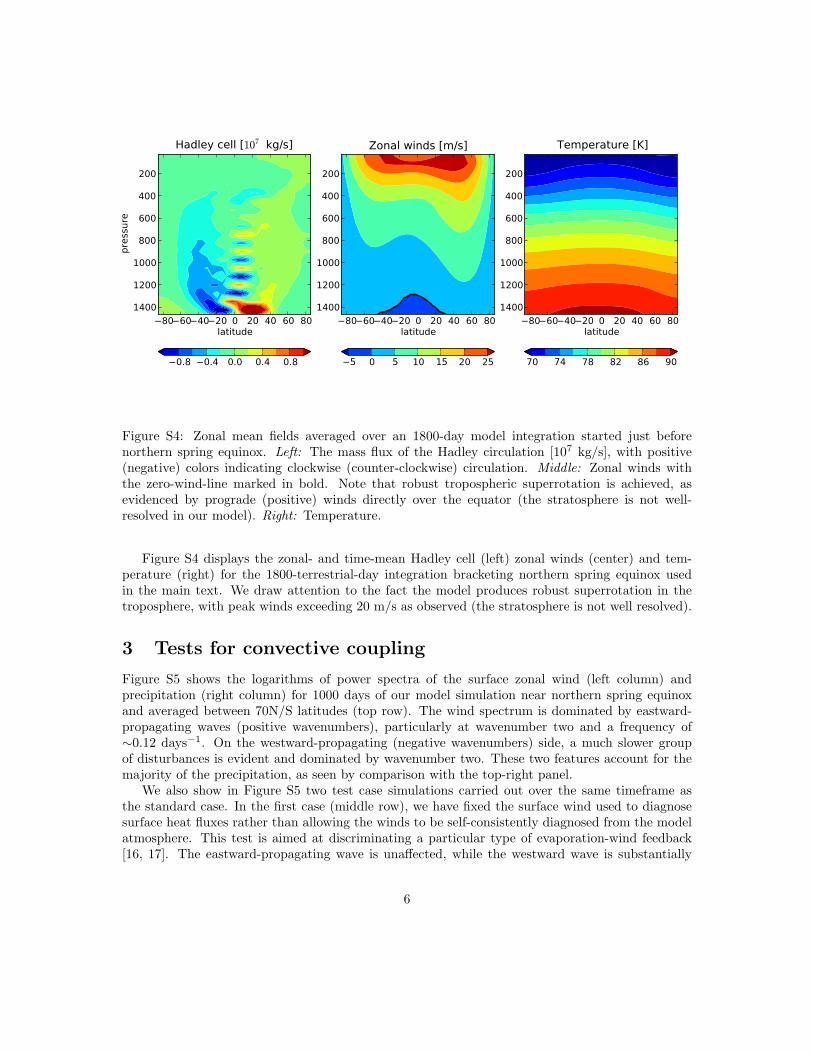
Figure S4: Zonal mean fields averaged over an 1800-day model integration started just beforenorthern spring equinox. Left: The mass flux of the Hadley circulation [107 kg/s], with positive(negative) colors indicating clockwise (counter-clockwise) circulation. Middle: Zonal winds withthe zero-wind-line marked in bold. Note that robust tropospheric superrotation is achieved, asevidenced by prograde (positive) winds directly over the equator (the stratosphere is not well-resolved in our model). Right: Temperature.

Figure S4 displays the zonal- and time-mean Hadley cell (left) zonal winds (center) and tem-perature (right) for the 1800-terrestrial-day integration bracketing northern spring equinox usedin the main text. We draw attention to the fact the model produces robust superrotation in thetroposphere, with peak winds exceeding 20 m/s as observed (the stratosphere is not well resolved).

3 Tests for convective coupling

Figure S5 shows the logarithms of power spectra of the surface zonal wind (left column) andprecipitation (right column) for 1000 days of our model simulation near northern spring equinoxand averaged between 70N/S latitudes (top row). The wind spectrum is dominated by eastward-propagating waves (positive wavenumbers), particularly at wavenumber two and a frequency of∼0.12 days−1. On the westward-propagating (negative wavenumbers) side, a much slower groupof disturbances is evident and dominated by wavenumber two. These two features account for themajority of the precipitation, as seen by comparison with the top-right panel.

We also show in Figure S5 two test case simulations carried out over the same timeframe asthe standard case. In the first case (middle row), we have fixed the surface wind used to diagnosesurface heat fluxes rather than allowing the winds to be self-consistently diagnosed from the modelatmosphere. This test is aimed at discriminating a particular type of evaporation-wind feedback[16, 17]. The eastward-propagating wave is unaffected, while the westward wave is substantially

6

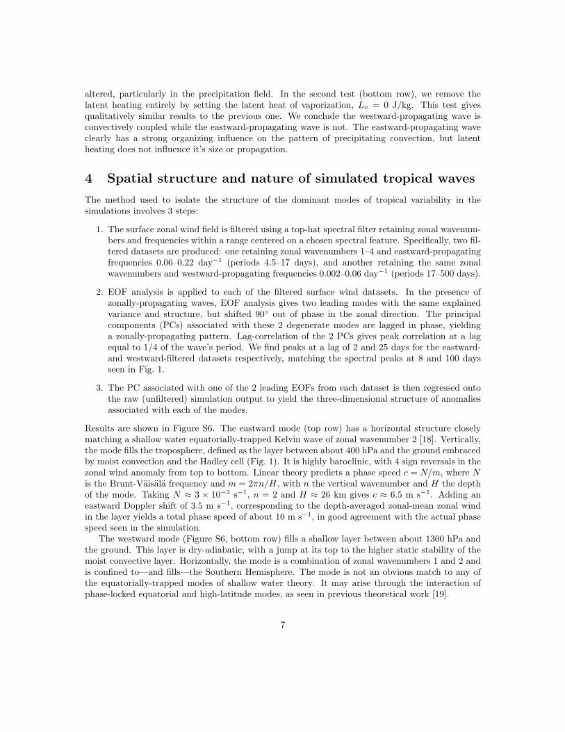
altered, particularly in the precipitation field. In the second test (bottom row), we remove thelatent heating entirely by setting the latent heat of vaporization, Lv = 0 J/kg. This test givesqualitatively similar results to the previous one. We conclude the westward-propagating wave isconvectively coupled while the eastward-propagating wave is not. The eastward-propagating waveclearly has a strong organizing influence on the pattern of precipitating convection, but latentheating does not influence it’s size or propagation.

4 Spatial structure and nature of simulated tropical waves

The method used to isolate the structure of the dominant modes of tropical variability in thesimulations involves 3 steps:

1. The surface zonal wind field is filtered using a top-hat spectral filter retaining zonal wavenum-bers and frequencies within a range centered on a chosen spectral feature. Specifically, two fil-tered datasets are produced: one retaining zonal wavenumbers 1–4 and eastward-propagatingfrequencies 0.06–0.22 day−1 (periods 4.5–17 days), and another retaining the same zonalwavenumbers and westward-propagating frequencies 0.002–0.06 day−1 (periods 17–500 days).

2. EOF analysis is applied to each of the filtered surface wind datasets. In the presence ofzonally-propagating waves, EOF analysis gives two leading modes with the same explainedvariance and structure, but shifted 90◦ out of phase in the zonal direction. The principalcomponents (PCs) associated with these 2 degenerate modes are lagged in phase, yieldinga zonally-propagating pattern. Lag-correlation of the 2 PCs gives peak correlation at a lagequal to 1/4 of the wave’s period. We find peaks at a lag of 2 and 25 days for the eastward-and westward-filtered datasets respectively, matching the spectral peaks at 8 and 100 daysseen in Fig. 1.

3. The PC associated with one of the 2 leading EOFs from each dataset is then regressed ontothe raw (unfiltered) simulation output to yield the three-dimensional structure of anomaliesassociated with each of the modes.

Results are shown in Figure S6. The eastward mode (top row) has a horizontal structure closelymatching a shallow water equatorially-trapped Kelvin wave of zonal wavenumber 2 [18]. Vertically,the mode fills the troposphere, defined as the layer between about 400 hPa and the ground embracedby moist convection and the Hadley cell (Fig. 1). It is highly baroclinic, with 4 sign reversals in thezonal wind anomaly from top to bottom. Linear theory predicts a phase speed c = N/m, where N

is the Brunt-Vaisala frequency and m = 2πn/H, with n the vertical wavenumber and H the depthof the mode. Taking N ≈ 3 × 10−3 s−1, n = 2 and H ≈ 26 km gives c ≈ 6.5 m s−1. Adding aneastward Doppler shift of 3.5 m s−1, corresponding to the depth-averaged zonal-mean zonal windin the layer yields a total phase speed of about 10 m s−1, in good agreement with the actual phasespeed seen in the simulation.

The westward mode (Figure S6, bottom row) fills a shallow layer between about 1300 hPa andthe ground. This layer is dry-adiabatic, with a jump at its top to the higher static stability of themoist convective layer. Horizontally, the mode is a combination of zonal wavenumbers 1 and 2 andis confined to—and fills—the Southern Hemisphere. The mode is not an obvious match to any ofthe equatorially-trapped modes of shallow water theory. It may arise through the interaction ofphase-locked equatorial and high-latitude modes, as seen in previous theoretical work [19].

7

Figure S5: Wavenumber-frequency power spectra of surface zonal winds (left) and precipitation(right) for 1000 days near northern spring equinox of our simulations. The top row is our standardcase analyzed in the main text. The middle and bottom rows display the no-evaporation-windfeedback test case and the zero-latent-heating test case, respectively (see text for more discussion).A slow, westward-propagating mode with a period of 100 days is present in the standard case, butit is substantially altered in the two test cases, indicating it is a convectively coupled wave. Thestrongest eastward-propagating mode at wavenumber 2 and frequency 0.12 day−1 is present in allcases, indicating it is not convectively coupled.

8

Figure S6: Spatial structure of the leading eastward (top row) and westward (bottom row) modesof variability. Left column shows an equatorial cross section of the zonal wind anomaly (red posi-tive, blue negative). Right column shows horizontal structure of the geopotential height anomaly(shading) and wind (arrows) at 1000 hPa (top) and 1400 hPa (bottom).

9

Figure S7: Zonal-mean precipitation rate normalized to the global- and annual-mean rate (a) duringone simulated Titan year of our GCM and (b) from the two-dimensional “moist” simulation of [20].The location of the northern spring equinox is marked by a dashed line.

5 Diagnostics of methane precipitation and evaporation

Figure S7 displays the zonal-mean precipitation rate normalized to the global- and annual-meanrate for our three-dimensional GCM (a) and two-dimensional simulation (b) [20]. The equato-rial chevrons are associated with the most intense zonal-mean equatorial precipitation during theequinoctial transition, which is marked by the dashed line. These are ephemeral.

Figure S8 shows the global- and annual-mean methane transport of our GCM, with positive (neg-ative) values indicating northward (southward) transport. The region between 10◦S and 10◦N lat-itudes experiences net divergence of transport, indicating climatological surface evaporation there.The ephemeral equatorial precipitation associated with chevrons in Figure S7 do not produce netaccumulation.

Figure S9 shows a space-time diagram of the model precipitation rate averaged between 10◦Sto 20◦S latitudes at a time corresponding to early 2008, roughly the location and time of the cloudoutburst observed by [21]. The eastward-propagating mode has a phase speed of roughly 8 m/s(solid line), which is in agreement with the Kelvin mode associated at a later model epoch with theequatorial chevron. The dashed line indicates 3 m/s, which was the observed propagation speed.The superposition of the Kelvin mode (symmetric about the equator) and the southern-hemisphereITCZ produces the eastward-propagating precipitation features.

Figure S10 displays precipitation rates and surface wind anomalies during a sequence of ap-proximately 3 terrestrial years bracketing NSE. The non-axisymmetric precipitation features areconcentrated at low latitudes, and show a clear progression from the south to the north with time.

10

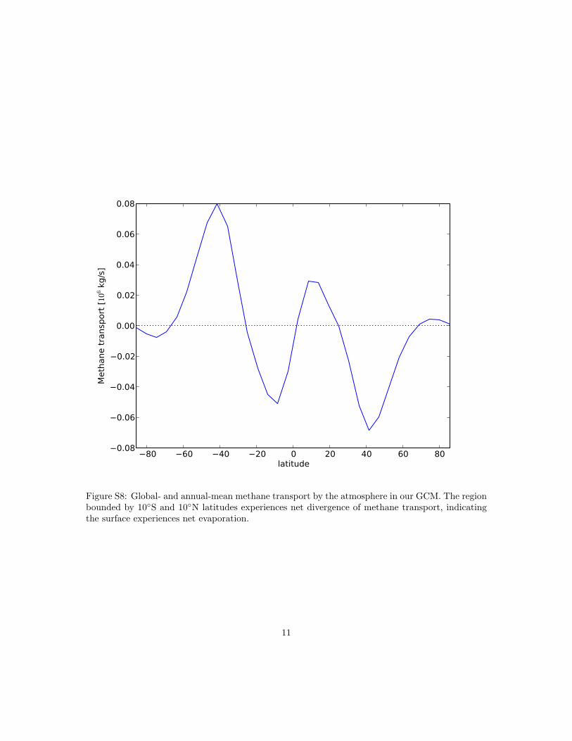
Figure S8: Global- and annual-mean methane transport by the atmosphere in our GCM. The regionbounded by 10◦S and 10◦N latitudes experiences net divergence of methane transport, indicatingthe surface experiences net evaporation.

11

Figure S9: Space-time diagram of precipitation averaged between 10◦S to 20◦S latitude during theepoch observed by [21]. The solid line indicates eastward motion at 8 m/s and the dashed line iseastward at 3 m/s.

12

Figure S10: Time sequence of precipitation rate (blue, normalized to the global- and time-meanrate) and surface wind anomalies (arrows) during a 3-terrestrial-year epoch bracketing NSE.

13

References

[1] Adamkovics, M., De Pater, I., Hartung, M. & Barnes, J. Evidence for condensed-phase methaneenhancement over Xanadu on Titan. Planetary and Space Science 57, 1586–1595 (2009).

[2] Adamkovics, M., Barnes, J., Hartung, M. & de Pater, I. Observations of a stationary mid-latitude cloud system on Titan. Icarus 208, 868–877 (2010).

[3] Karkoschka, E. & Tomasko, M. Methane absorption coefficients for the jovian planets fromlaboratory, Huygens, and HST data. Icarus 205, 674–694 (2010).

[4] Tomasko, M. et al. Measurements of methane absorption by the descent imager/spectralradiometer (DISR) during its descent through Titan’s atmosphere. Planetary and Space Science

56, 669–707 (2008).

[5] Turtle, E. et al. Seasonal changes in Titan’s meteorology. Geophys. Res. Lett. 38, L03203(2011).

[6] Barth, E. & Toon, B. O. Methane, ethane, and mixed clouds in Titan’s atmosphere: Propertiesderived from microphysical modeling. Icarus 182, 230–250 (2006).

[7] Samuelson, R. E. & Mayo, L. A. Steady-state model for methane condensationin titan’s troposphere. Planetary and Space Science 45, 949–958 (1997). URLhttp://www.sciencedirect.com/science/article/pii/S0032063397000895.

[8] Whalley, E. & McLaurin, G. E. Refraction halos in the solar system. i. halos from cubic crystalsthat may occur in atmospheres in the solar system. J. Opt. Soc. Am. A 1, 1166–1170 (1984).URL http://josaa.osa.org/abstract.cfm?URI=josaa-1-12-1166.

[9] Tokano, T. et al. Methane drizzle on Titan. Nature 442, 432–435 (2006).

[10] Barth, E. L. & Toon, O. B. Microphysical modeling of ethane iceclouds in titan’s atmosphere. Icarus 162, 94–113 (2003). URLhttp://www.sciencedirect.com/science/article/pii/S0019103502000672.

[11] Mitchell, J., Pierrehumbert, R., Frierson, D. & Caballero, R. The impact of methane thermo-dynamics on seasonal convection and circulation in a model Titan atmosphere. Icarus 203,250–264 (2009).

[12] Gordon, C. & Stern, W. A description of the GFDL global spectral model. Mon. Wea. Rev

110, 625–644 (1982).

[13] McKay, C., Pollack, J. & Courtin, R. The greenhouse and antigreenhouse effects on Titan.Science 253, 1118–1121 (1991).

[14] Frierson, D. M. W., Held, I. M. & Zurita-Gotor, P. A gray-radiation aquaplanet moist GCM.Part I: Static stability and eddy scale. Journal of the Atmospheric Sciences 63, 2548–2566(2006).

[15] Tokano, T. Meteorological assessment of the surface temperatures on Titan: constraints onthe surface type. Icarus 173, 222–242 (2005).

14

[16] Emanuel, K. An air-sea interaction model of intraseasonal oscillations in the tropics. Journal

of the Atmospheric Sciences 44, 2324–2340 (1987).

[17] Neelin, J. & Held, I. Modeling tropical convergence based on the moist static energy budget.Monthly Weather Review 115, 3–12 (1987).

[18] Matsuno, T. Quasi-geostrophic motions in the equatorial area. J. Meteor. Soc. Japan 44,25–42 (1966).

[19] Mitchell, J. & Vallis, G. The transition to superrotation in terrestrial atmospheres. J. Geophys.

Res. 115, E12008 (2010).

[20] Mitchell, J., Pierrehumbert, R., Frierson, D. & Caballero, R. The dynamics behind Titan’smethane clouds. Proc. Natl. Acad. Sci. USA 103, 18421—18426 (2006).

[21] Schaller, E., Roe, H., Schneider, T. & Brown, M. Storms in the tropics of Titan. Nature 460,873–875 (2009).

15