localization of wireless sensor networks using mobile ...721942/s4329529_final... · saiful rizal...
TRANSCRIPT

Localization of Wireless Sensor Networks using Mobile Anchor Nodes
Izanoordina Ahmad
MSc Mechatronics (Signal and Systems)
A thesis submitted for the degree of Doctor of Philosophy at
The University of Queensland in 2018
School of Information Technology and Electrical Engineering

i
Abstract
Wireless sensor networks (WSNs) are an important class of pervasive computing environments.
WSNs have been described as a new instrument for gathering data about the natural world, extending
the reach of our human senses. WSN applications are dominated by constrained resources such as
energy, computing power, storage and communications bandwidth.
An important aspect of WSN operation is the geolocation of all the sensor nodes. Automatically
determining sensor position after deployment will improve the reporting of the origin of events in
indoor and outdoor applications, in areas such as environmental monitoring, target tracking and
disaster relief operations. This thesis explores the use of a mobile anchor moving through a sensor
field to localize the nodes in an outdoor setting.
The scope of possible experiments with mobile anchor nodes for localization is almost endless. A
motivating scenario of air-dropped sensors, and an airborne mobile anchor node will be used to define
a focussed set of experiments that have a real application outcome while still providing useful
information for other scenarios.
With regards to the previous work done by others, little attention has been paid in the literature to
how many beacon packets need to be sent by the mobile anchor node, what type of localization
algorithm gives the best performance, what path the mobile anchor node should take, what are the
geometric parameters of the path, and whether adding range-estimates between blind nodes is
beneficial. In answering these questions, this thesis makes several contributions.
Firstly, a new algorithm called Volume-based Probabilistic Multi-Lateration (VPML) is devised
which can reduce localization errors by up to 75%. Secondly, a simulation framework is devised
which can answer questions such as the most suitable flight-path for a mobile anchor. The
contributions obtained from the simulation results extend beyond just the VPML algorithm, and
include findings about the best beacon placements. Results show that by having well-placed anchors,
a low ranging uncertainty can be achieved with fewer anchors and a shorter travel distance. Thirdly,
the new algorithm (VPML) together with an optimized flight path (alternate 10m/13m height square
grid, 10m spacing) is able to localize air-dropped sensor nodes within a few metres using inherently
inaccurate RSSI-based range estimates from the mobile beacon. Finally, a technique for cooperative
localization is identified which can reduce the flight path by 80% while still maintaining acceptable
localization accuracy. This technique allows decisions to be made about operational requirements for
the use of a mobile anchor prior to deployment.

ii
Declaration by author
This thesis is composed of my original work, and contains no material previously published or written
by another person except where due reference has been made in the text. I have clearly stated the
contribution by others to jointly-authored works that I have included in my thesis.
I have clearly stated the contribution of others to my thesis as a whole, including statistical assistance,
survey design, data analysis, significant technical procedures, professional editorial advice, financial
support and any other original research work used or reported in my thesis. The content of my thesis
is the result of work I have carried out since the commencement of my higher degree by research
candidature and does not include a substantial part of work that has been submitted to qualify for the
award of any other degree or diploma in any university or other tertiary institution. I have clearly
stated which parts of my thesis, if any, have been submitted to qualify for another award.
I acknowledge that an electronic copy of my thesis must be lodged with the University Library and,
subject to the policy and procedures of The University of Queensland, the thesis be made available
for research and study in accordance with the Copyright Act 1968 unless a period of embargo has
been approved by the Dean of the Graduate School.
I acknowledge that copyright of all material contained in my thesis resides with the copyright
holder(s) of that material. Where appropriate I have obtained copyright permission from the copyright
holder to reproduce material in this thesis and have sought permission from co-authors for any jointly
authored works included in the thesis.

iii
Publications during candidature
Peer Reviewed Conference Papers
I. Ahmad, N. Bergmann, R. Jurdak, and B. Kusy, "Experiments on localization of wireless sensors
using airborne mobile anchors," in IEEE Conference on Wireless Sensors (ICWiSe), pp. 1-6: IEEE.
2015, DOI: 10.1109/ICWISE.2015.7380344
I. Ahmad, N. W. Bergmann, R. Jurdak, and B. Kusy, "Towards probabilistic localization using
airborne mobile anchors," in IEEE International Conference on Pervasive Computing and
Communication Workshops (PerCom Workshops), pp. 1-4: IEEE. 2016, DOI:
10.1109/PERCOMW.2016.7457052
I. Ahmad, "Localization of wireless sensor networks using a mobile beacon," in IEEE International
Conference on Pervasive Computing and Communication Workshops (PerCom Workshops), pp. 1-4:
IEEE. 2016, DOI: 10.1109/PERCOMW.2016.7457081
Publications included in this thesis
No publications included.

iv
Contributions by others to the thesis
No contributions by others.
Statement of parts of the thesis submitted to qualify for the award of another degree
None.
Research Involving Human or Animal Subjects
No animal or human participants were involved in this research.

v
Acknowledgements
My complex, yet exciting journey as a PhD student would not have been possible without the
support and assistance from certain special individuals and parties. I would first like to express my
greatest gratitude to my dedicated supervisors, Professor Neil Bergmann, Professor Raja Jurdak and
Dr. Branislav Kusy for their valuable guidance and patience in helping me throughout the process of
researching and writing of this thesis. I could not have asked for better supervisors and mentors to
assist me with my PhD program.
A big thank you to my sponsorship, MARA (Majlis Amanah Rakyat) and UniKL (Universiti Kuala
Lumpur). With their care and financial assistance, I am able to make it this far in the program and is
able to reach my goal as a doctoral student.
I would also like to extend my special thanks to the research group and colleagues from CSIRO
and University of Queensland, Australia for their incredible collaboration, and for always being there
when I needed any help.
Most importantly, I wish to present my wholeheartedly appreciation to my supportive husband,
Saiful Rizal Shafie, my beloved children, Syahmi, Shasmeen, Iris and Iman, my late parents
especially my mom, my parents-in-law and my family members. They have not only been supporting
and encouraging me to do my best, but have been there every step of the way. Without them, I would
not be who I am today.

vi
Financial support
Scholarship support from MARA (Majlis Amanah Rakyat) and UniKL (Universiti Kuala Lumpur) in
Malaysia is gratefully acknowledged.
Financial assistance for attendance at conferences from School of ITEE, University of Queensland,
and from CSIRO/Data61 is also gratefully acknowledged.

vii
Keywords
Localization, wireless sensor networks, multilateration, geometric sensitivity, cooperative
localization.
Australian and New Zealand Standard Research Classifications (ANZSRC)
ANZSRC code: 080504, Ubiquitous Computing, 50%
ANZSRC code: 080607, Information Engineering and Theory, 50%
Fields of Research (FoR) Classification
FoR code: 0805, Distributed Computing, 50%
FoR code: 0806, Information Systems, 50%

viii
Table of Contents Abstract ................................................................................................................................................. i
Declaration by author ........................................................................................................................... ii
Publications during candidature .......................................................................................................... iii
Publications included in this thesis ..................................................................................................... iii
Contributions by others to the thesis ................................................................................................... iv
Statement of parts of the thesis submitted to qualify for the award of another degree ....................... iv
Research Involving Human or Animal Subjects ................................................................................. iv
Acknowledgements .............................................................................................................................. v
Financial support ................................................................................................................................. vi
Keywords ........................................................................................................................................... vii
Australian and New Zealand Standard Research Classifications (ANZSRC) ................................... vii
Fields of Research (FoR) Classification ............................................................................................ vii
List of Figures ................................................................................................................................... xiv
List of Tables ................................................................................................................................... xvii
List of Abbreviations ........................................................................................................................ xix
CHAPTER 1 ....................................................................................................................................... 1
INTRODUCTION .............................................................................................................................. 1
1.1 Localization: terminology. .................................................................................................... 2
1.2 Motivation. ............................................................................................................................ 2
1.3 Organization of the manuscript. ............................................................................................ 5
CHAPTER 2 ....................................................................................................................................... 6
LITERATURE REVIEW.................................................................................................................. 6
2.1 Distance-based Wireless Localization Techniques. .............................................................. 7
2.1.1 Previous Work with Airborne Anchors. ......................................................................... 7
2.1.2 Range-free localization. ............................................................................................... 10
2.1.2.1 Centroid system. ........................................................................................................... 12
2.1.2.2 Distance Vector (DV Hop). .......................................................................................... 12

ix
2.1.2.3 Hop Terrain. ................................................................................................................ 12
2.1.2.4 Appropriate Point in Triangulation (APIT). ................................................................ 13
2.1.3 Range-based algorithms. ............................................................................................. 13
2.1.3.1 Ranging signals. ........................................................................................................... 13
2.1.3.2 Time of Arrival (ToA). .................................................................................................. 14
2.1.3.3 Time Difference of Arrival (TDoA). ............................................................................. 14
2.1.3.4 Received Signal Strength Indicator (RSSI). ................................................................. 15
2.1.4 RF propagation models, advantages and disadvantages............................................. 16
2.1.4.1 Probability distribution using Log normal shadowing model. .................................... 17
2.1.4.2 RSSI and its relationship to distance. .......................................................................... 19
2.2 Angle of Arrival (AoA). ...................................................................................................... 20
2.2.1 Angle with range-based localization (Hybrid system). ................................................ 20
2.3 Implementation of GPS-based localization on mobile anchor node. .................................. 21
2.4 Multilateration algorithm for localization. .......................................................................... 22
2.4.1 Deterministic and Probabilistic Multilateration.......................................................... 23
2.5 Gradient descent solution of multilateration. ...................................................................... 24
2.6 Beacon geometric sensitivity and its placement. ................................................................. 25
2.6.1 Flip ambiguity. ............................................................................................................. 26
2.7 Indoor versus outdoor localization. ..................................................................................... 27
2.8 Centralized and distributed computation. ............................................................................ 29
2.9 Static anchor node versus mobile anchor node. .................................................................. 30
2.10 Path planning for the mobile anchor node. .......................................................................... 32
2.10.1 Random trajectories. .................................................................................................... 32
2.10.2 Dynamic trajectories. ................................................................................................... 32
2.10.3 Static trajectories. ........................................................................................................ 32
2.11 Cooperative localization using inter blind node range measurement. ................................. 35
2.11.1 Comparison between non-cooperative and cooperative localization. ......................... 35
2.11.2 Implementation of cooperative localization. ................................................................ 36

x
2.12 Localization performance evaluation. ................................................................................. 37
2.12.1 Accuracy and localization error. ................................................................................. 37
2.12.2 Communication and computational cost...................................................................... 38
2.12.3 Number of anchor nodes. ............................................................................................. 38
2.13 Energy efficiency. ............................................................................................................... 39
2.14 Summary. ............................................................................................................................ 39
CHAPTER 3 ..................................................................................................................................... 42
RESEARCH QUESTIONS ............................................................................................................. 42
3.1 Gap analysis. ....................................................................................................................... 42
3.2 Research questions and methodologies. .............................................................................. 44
3.2.1 Preliminary experiment. ............................................................................................... 44
3.2.2 RQ1: How does the localization performance of a mobile anchor vary with different
numbers of beacon packets, and how does it compare with the use of fixed anchors, or
combinations of fixed and mobile anchors? ............................................................................... 45
3.2.2.1 Framework. .................................................................................................................. 45
3.2.3 RQ2: What is the localization performance of probabilistic localization algorithms
compared to deterministic algorithms, and how does this vary with the number of beacon
packets? 46
3.2.3.1 Framework. .................................................................................................................. 46
3.2.4 RQ3: How does the mobile anchor’s trajectory influence the performance and what is
the most suitable trajectory based on the proposed scenario? How does performance vary with
the number of beacons sent and the positions that they are sent from? ..................................... 47
3.2.4.1 Framework. .................................................................................................................. 47
3.2.5 RQ4: What is the relative localization performance of adding inter-blind node range
estimates to anchor range estimates? ......................................................................................... 47
3.2.5.1 Framework. .................................................................................................................. 48
3.3 Summary. ............................................................................................................................ 48
CHAPTER 4 ..................................................................................................................................... 49
PRELIMINARY EXPERIMENTS FOR PROPAGATION MODEL ........................................ 49

xi
4.1 Radio parameters through preliminary real outdoor experiment. ....................................... 50
4.1.1 Path loss mean. ............................................................................................................ 50
4.1.2 Standard Deviation. ..................................................................................................... 52
CHAPTER 5 ..................................................................................................................................... 54
LOCALIZATION ACCURACY VERSUS THE NUMBER OF MOBILE ANCHOR
POSITIONS ...................................................................................................................................... 54
5.1 Deterministic Multilateration (DML). ................................................................................. 55
5.2 Experimental setup. ............................................................................................................. 55
5.3 Results. ................................................................................................................................ 57
5.3.1 Localization of the blind node using random mobile anchor node positions. ............. 57
5.3.2 Localization of the blind node using designated flight path. ....................................... 58
5.3.3 Localization of the blind node using fixed static anchors. ........................................... 59
5.3.4 Localization of the blind node using a combination of fixed and mobile anchor
node. 61
5.3.4.1 Comparison of RSSI variabilities for fixed, mobile and combination anchor. ............ 62
5.3.5 Localization of the blind node at poor geometrical position. ...................................... 64
5.4 Analysis. .............................................................................................................................. 65
CHAPTER 6 ..................................................................................................................................... 67
PROBABILISTIC MULTILATERATION .................................................................................. 67
6.1 Probabilistic localization algorithms. .................................................................................. 67
6.1.1 Linear Probabilistic Multilateration (LPML). ............................................................. 68
6.1.2 Volume Probabilistic Multilateration (VPML). ........................................................... 70
6.2 Experimental setup. ............................................................................................................. 74
6.3 Results. ................................................................................................................................ 75
6.3.1 Localization single blind node localization at favourable and poor geometrical
position using DML and VPML. ................................................................................................. 75
6.3.2 Localization for single blind node localization using DML, LPML and VPML. ......... 78
6.3.2.1 DML versus LPML and VPML for low RSSI variability. ............................................ 78

xii
6.3.2.2 DML versus LPML and VPML for medium RSSI variability....................................... 80
6.3.2.3 DML versus LPML and VPML for high RSSI variability. ........................................... 81
6.4 Analysis. .............................................................................................................................. 82
CHAPTER 7 ..................................................................................................................................... 84
GEOMETRIC SENSITIVITY AND TRAJECTORY OF MOBILE ANCHOR NODE .......... 84
7.1 Introduction. ........................................................................................................................ 84
7.2 Experimental Setup 1. ......................................................................................................... 86
7.2.1 Methodology................................................................................................................. 86
7.2.2 Results. ......................................................................................................................... 86
7.3 Experimental Setup 2. ......................................................................................................... 87
7.3.1 Methodology................................................................................................................. 87
7.3.2 Results. ......................................................................................................................... 88
7.4 Experimental Setup 3. ......................................................................................................... 89
7.4.1 Methodology................................................................................................................. 89
7.4.2 Results. ......................................................................................................................... 91
7.5 Experimental Setup 4. ......................................................................................................... 92
7.5.1 Methodology................................................................................................................. 92
7.5.2 Results. ......................................................................................................................... 92
7.6 Experimental Setup 5. ......................................................................................................... 96
7.6.1 Methodology................................................................................................................. 97
7.6.2 Results. ......................................................................................................................... 97
7.7 Conclusions. ...................................................................................................................... 105
CHAPTER 8 ................................................................................................................................... 106
COOPERATIVE LOCALIZATION ........................................................................................... 106
8.1 Inter-node cooperative localization algorithm. ................................................................. 106
8.2 Wide Spacing Cooperation Localization. .......................................................................... 106
8.2.1 Experimental Setup 1. ................................................................................................ 106
8.2.2 Results Varying Node Density.................................................................................... 110

xiii
8.2.3 Results using 60m spacing. ........................................................................................ 116
8.2.4 Changing Minimum Number of Anchors. .................................................................. 117
8.3 Edge-Based Cooperative Localization. ............................................................................. 122
8.3.1 Experimental Setup 2. ................................................................................................ 122
8.3.2 Results for 200 Blind Nodes. ...................................................................................... 123
8.3.3 Results for 1000 Blind Nodes. .................................................................................... 126
8.4 Analysis. ............................................................................................................................ 127
CHAPTER 9 ................................................................................................................................... 129
CONCLUSION, CONTRIBUTIONS AND FUTURE WORK ................................................. 129
9.1 Research Question 1 (Localization accuracy vs. number of mobile anchor positions). ... 129
9.2 Research Question 2 (Probabilistic Multilateration). ........................................................ 130
9.3 Research Question 3 (Geometric sensitivity and trajectory of mobile anchor node). ....... 130
9.4 Research Question 4 (Cooperative localization). .............................................................. 131
9.5 Original Contributions. ...................................................................................................... 131
9.6 Future Research. ................................................................................................................ 132
References ....................................................................................................................................... 133
Appendix A. .................................................................................................................................... 143
Appendix B ..................................................................................................................................... 147
Appendix C ..................................................................................................................................... 172
Appendix D ..................................................................................................................................... 176
Appendix E ..................................................................................................................................... 192
Appendix F ..................................................................................................................................... 200
xiv
List of Figures
Figure 1.1: Localization using mobile anchor node. ........................................................................... 3
Figure 2.1: Localization process .......................................................................................................... 7
Figure 2.2: Wireless localization techniques. .................................................................................... 10
Figure 2.3: Multilateration using TDoA and ToA measurements with hyperbolae and circle
respectively as possible emitter location. ........................................................................................... 15
Figure 2.4: Log normal distribution of distances for packets with RSSI=83. ................................... 18
Figure 2.5: Intersection points of spheres in Multilateration ............................................................. 23
Figure 2.6: Flip ambiguities ............................................................................................................... 27
Figure 2.7: Signal fingerprinting work by collecting the RSSI values from multiple WiFi access points
or base stations to generate a unique signature of an area ................................................................. 29
Figure 2.8: Static path planning for (a) Scan (b) Hilbert (c) Circle and (d) S-Curves with individual
path length .......................................................................................................................................... 33
Figure 2.9: Non-Cooperative localization .......................................................................................... 35
Figure 2.10: Cooperative localization ................................................................................................ 36
Figure 2.11: Localization of wireless sensor networks using mobile anchor nodes .......................... 41
Figure 4.1: Camazotz prototype device without battery and solar panel ........................................... 50
Figure 4.2: Path Loss mean versus logarithm of distance.................................................................. 51
Figure 4.3: Histogram and log-normal shadowing distribution of the reading at 20 metres ............. 52
Figure 5.1: The actual and estimated blind node’s location on the ground with designated position of
anchor node ........................................................................................................................................ 57
Figure 5.2: Localization error versus number of mobile anchor node with random positions for blind
node deployed on the ground ............................................................................................................. 58
Figure 5.3: Average localization error in metres for 15 mobile anchors with designated flightpath
positions for different RSSI variability .............................................................................................. 59
Figure 5.4: Localization error using four fixed anchors only for blind node at 25,25,0 .................... 60
Figure 5.5: Localization error using four fixed anchors only for blind node at 40, 25, 0 .................. 60
Figure 5.6: Localization of fixed blind node on the ground using combination of fixed anchor and
designated position of mobile anchor node........................................................................................ 61
Figure 5.7: Comparison of 4 fixed anchors, the best 4 to 15 mobile anchor node positions and the best
4 to 15 combination of fixed and mobile anchor positions with low variability ............................... 63
Figure 5.8: Comparison of 4 fixed anchors, the best 4 to 15 mobile anchor node positions and the best
4 to 15 combination of fixed and mobile anchor positions with medium variability ........................ 63

xv
Figure 5.9: Comparison of 4 fixed anchors, the best 4 to 15 mobile anchor node positions and the best
4 to 15 combination of fixed and mobile anchor positions with high variability .............................. 64
Figure 5.10: Localization of fixed blind node at poor geometrical position using fixed anchor and
designated position of mobile anchor node........................................................................................ 65
Figure 6.1: 3 dimensional spatial PDF ............................................................................................... 71
Figure 6.2: Comparison between DML and VPML .......................................................................... 72
Figure 6.3: Comparison between LPML and VPML ......................................................................... 73
Figure 6.4: Median localization error using N from 15 designated mobile anchor node positions with
DML and VPML for node in favourable position. 10/90 percentile ranges also shown ................... 76
Figure 6.5: Median localization error using N from 15 designated mobile anchor node positions with
DML and VPML for node in unfavourable position. 10/90 percentile ranges shown ....................... 77
Figure 6.6: DML versus LPML and VPML for standard deviation of 1dB ...................................... 79
Figure 6.7: DML versus LPML and VPML for standard deviation of 3.36dB ................................. 80
Figure 6.8: DML versus LPML and VPML for standard deviation of 5dB ...................................... 82
Figure 7.1: Median error (m) versus number of iterations for 5 trials ............................................... 87
Figure 7.2: Comparison between height for blind node 127,192,0 and 500,500,0 ............................ 88
Figure 7.3: Square grid path with 5m beacon spacing and alternate layers of 10m and 11m height 90
Figure 7.4: Square grid path with 30m beacon spacing and laternate layers of 10m and 13m
height .................................................................................................................................................. 90
Figure 7.5: Comparison between localization errors versus beacon distance interval using 20 beacons
............................................................................................................................................................ 91
Figure 7.6: Comparison of average localization error between size for blind node 5 (500,500,0) ... 93
Figure 7.7: Comparison of average localization error between size for blind node (0,0,0) .............. 94
Figure 7.8: Comparison of average localization error between size for blind node (142, 439, 0) ... 95
Figure 7.9: Anchor positions according to the strongest RSSI based on 5 metre spacing ................. 98
Figure 7.10: Anchor positions according to the strongest RSSI based on 10 metre spacing ............. 99
Figure 7.11: Anchor positions according to the strongest RSSI based on 20 metre spacing ........... 100
Figure 8.1: Localization using 50 metres spaces between beacons in square grid path for a) 50 b) 100
and c) 200 blind nodes ..................................................................................................................... 108
Figure 8.2: Median localization error for 50 blind nodes based on generation ............................... 110
Figure 8.3: Localized and unlocalized (UL) nodes through generation (G1-G2) for 50 blind
nodes ................................................................................................................................................ 111
Figure 8.4: Average localization error for 100 blind nodes based on generation ............................ 112
xvi
Figure 8.5: Localized and unlocalized (UL) nodes through generation (G1-G2) for 100 blind
nodes ................................................................................................................................................ 113
Figure 8.6: Average localization error for 200 blind nodes based on generation ............................ 114
Figure 8.7: Localized and unlocalized (UL) nodes through generation (G1-G2) for 200 blind
nodes ................................................................................................................................................ 115
Figure 8.8: Average localization error for 200 blind node based on generation using 60 metre
spaces ............................................................................................................................................... 116
Figure 8.9: Localized and unlocalized (UL) nodes through generation (G1-G2) for 200 blind nodes
using 60 metres spaces ..................................................................................................................... 117
Figure 8.10: Average localization error for 200 blind nodes based on generation using (a) 6, (b) 7 and
(c) 8 minimum anchor positions ...................................................................................................... 119
Figure 8.11: Local anchors for each generation (G1 to G3) using 7 anchor positions .................... 120
Figure 8.12: Local anchors for each generation (G1 to G3) using 8 anchor positions .................... 121
Figure 8.13: Localization using 50 metres spacing between beacons using 200 blind nodes and edge
path planning .................................................................................................................................... 122
Figure 8.14: Localization error for 200 blind nodes based on generation using edge path panning 124
Figure 8.15: Localized and unlocalized (UL) nodes through generation (G1-G2) for 200 blind nodes
using edge path planning.................................................................................................................. 125
Figure 8.16: Localization for 1000 blind nodes using edge path planning ...................................... 126
Figure 8.17: Localized blind nodes through generation (G1-G4) for 200 blind nodes using edge path
planning ............................................................................................................................................ 127

xvii
List of Tables
Table 2.1: Previous works with Airborne anchors ............................................................................... 9
Table 4.1: Path loss mean for each distance ...................................................................................... 51
Table 4.2: Standard Deviation ........................................................................................................... 52
Table 4.3: Parameters for simulation ................................................................................................. 53
Table 5.1: Average localization error in metres for 15 mobile anchors with random positions for
different RSSI variability ................................................................................................................... 58
Table 5.2: Localization error for 15 designated mobile anchor node at different RSSI variability ... 59
Table 5.3: Localization error using four fixed anchors for blind node 25,25,0 ................................ 60
Table 5.4: Localization error using four fixed anchors for blind node 40,25,0 ................................. 61
Table 5.5: Localization error for 15 anchors at different RSSI variability ........................................ 62
Table 5.6: New position of anchor nodes (fixed and mobile anchor) based on the shortest estimated
distance in metre ................................................................................................................................ 62
Table 5.7: Localization accuracy for different scenario with low variability .................................... 63
Table 5.8: Localization accuracy for different scenario with medium variability ............................. 64
Table 5.9: Localization accuracy for different scenario with high variability ................................... 64
Table 5.10: Localization accuracy for blind node at poor geometrical position ................................ 65
Table 6.1: Localization median error (metres) and standard deviation (metres) for favourable blind
node position ...................................................................................................................................... 76
Table 6.2: Localization median error (metres) and standard deviation (metres) for unfavourable blind
node position ...................................................................................................................................... 77
Table 6.3: The median error and standard deviations (SD) of errors (in metres) for DML, LPML and
VPML for standard deviation of 1 dB ............................................................................................... 79
Table 6.4: The median error and standard deviations (SD) of errors (in metres) for DML, LPML and
VPML for standard deviation of 3.36dB ........................................................................................... 81
Table 6.5: The median error and standard deviations (SD) of errors (in metres) for DML, LPML and
VPML for standard deviation of 5dB ................................................................................................ 82
Table 7.1: Position of 25 blind nodes (in metres) .............................................................................. 85
Table 7.2: Median errors (m) for each of 5 trials ............................................................................... 87
Table 7.3: Average localization error for blind node 127, 192, 0 and 500, 500, 0 ............................ 89
Table 7.4: Comparison of average localization error with 20 beacons based on beacon distance
interval and height .............................................................................................................................. 92
Table 7.5: Comparison of average localization error between size for blind node 5 (500,500,0) ..... 93

xviii
Table 7.6: Comparison of average localization error between size for blind node (0,0,0) ................ 94
Table 7.7: Comparison of average localization error between size for blind node (142,439,0) ........ 95
Table 7.8: Path characteristics for different grid spacing .................................................................. 96
Table 7.9: Anchor positions according to the strongest RSSI based on 5 metre spacing .................. 98
Table 7.10: Anchor positions according to the strongest RSSI based on 10 metre spacing .............. 99
Table 7.11: Anchor positions according to the strongest RSSI based on 20 metre spacing ............ 100
Table 7.12: Angle between beacons for 5m spacing ....................................................................... 101
Table 7.13: Angle between beacons for 10m spacing ..................................................................... 102
Table 7.14: Angle between beacons for 20m spacing ..................................................................... 103
Table 8.1: Positions of mobile anchor for square grid path ............................................................. 109
Table 8.2: Local and mobile anchor for localized blind node 13 and 42 by using 200 blind nodes 115
Table 8.3: Performance versus Node Density .................................................................................. 116
Table 8.4: Localization Errors versus Minimum Anchors ............................................................... 118
Table 8.5: Position of mobile anchor node for edge path ................................................................ 123

xix
List of Abbreviations
2D Two Dimensions
3D Three Dimensions
3D-ADAL Three-Dimensional Azimuthally Defined Area Localization
AGPS Assisted GPS
AoA Angle of Arrival
APIT Appropriate Point in Triangulation
COLA Complexity-Reduced 3D Trilateration Localization Approach
CRLB Cramer Rao Low Bound
dBm decibels referenced to 1mW power
DGPS Differential GPS
DML Deterministic Multilateration
DREAMS Deterministic beAcon Mobility Scheduling
DV Distance Vector
ECG Electrocardiogram
FLS Fuzzy Logic System
GDM Gradient descent method
GDOP Geometric Dilution of Precision
GPS Global Positioning System
HPSO Hybrid-Particle Swarm Optimisation
IMU Inertial Measurement Unit
IoT Internet of Things
LMAT Mobile Anchor node based on Trilateration
LNMS Log Normal Shadowing Model
LoS Line of Sight
LPML Linear Probabilistic Multilateration

xx
LS Least square
MAALRH Mobile Anchor Assisted Localization Algorithm based on Regular Hexagon
MAE Mean Absolute Error
MBAL Mobile anchor node Assisted Localization
ML Maximum Likelihood
MRS Multirobot System
N Number
NLOS Non-line of sight
PDF Probability Distribution Function
PS Push-sum
ReNLoc Relaid Ranging Localization
RF Radio Frequency
RMSE Root Mean Square Error
RSSI Received Signal Strength Indicator
SBLS Sound-Based Localization System
SMAL Single Mobile Anchor Location
TDoA Time Difference of Arrival
ToA Time of Arrival
ToF Time of Flight
UAV Unmanned Aerial Vehicle
UGV Utility Ground Vehicle
VPML Volume Probabilistic Multilateration
WiFi Wireless Fidelity
WSNs Wireless sensor networks

1
CHAPTER 1
INTRODUCTION
Wireless sensor networks (WSNs) are an important class of pervasive computing environments.
As one of the important technologies in the Internet of Things (IoT), WSNs have been described as a
new instrument for gathering data about the natural world, extending the reach of our human senses.
WSNs are composed of intercommunicating networks of smart sensor nodes, they are deployed in
real environments and usually they are small, low-cost devices with limited processing capabilities.
The applications of WSN are enormous, such as in military, civil and environmental applications [1].
In environmental monitoring, the sensors can detect scalar features like temperature or multimedia
features like audio and video. WSNs can be used to detect bushfires, to track the movements of
animals to observe their habits, to observe plant growth, or to monitor soil movement. In traffic
control systems, sensors are used to monitor vehicle movements. In industrial monitoring, sensors
can be used to monitor a production line, to reduce downtime. Medical sensors are used to monitor
the condition of patients such as their blood pressure, blood sugar level, or electrocardiogram (ECG).
These sensors often simply store and forward the information for subsequent data analysis.
WSN applications are dominated by constrained resources such as energy, computing power,
storage and communications bandwidth [2]. The issues of hardware and operating system,
deployment, wireless sensors and actuators, time synchronization and localization can affect the
design and performance of the overall network.
In some cases, sensors are deployed in remote areas without significant communications
infrastructure. For example, sensors could be dropped in a forest to monitor the progress of a bushfire.
Another useful example from our laboratory is in Springbrook rainforest where a long term WSN-
based monitoring system has been deployed to monitor forest regrowth after previous logging in the
area, to better understand how forests regenerate [3].
In cases where sensors are remotely deployed, automatically determining the precise geolocation
of sensor nodes after deployment is often critical for the reporting of origin of events in indoor and
outdoor applications. For instance, without the precise location of temperature readings in a forest,
the location of a bushfire cannot be detected. To date, many algorithms have been proposed to solve
the issues of device localization. Many of the algorithms that have been published are suitable for
specific scenarios, such as indoor localization of mobile phones or outdoor localization with using a
small number of geo-located anchor nodes. Additionally, some localization technologies such as the

2
Global Positioning System (GPS) are relatively expensive and not always available. Factors of energy
consumption, communication cost and require location accuracy also need to be considered while
choosing an appropriate localization algorithm.
1.1 Localization: terminology.
Many different objects need to be localized in many different situations. For instance, a tennis
player uses stereo vision to localize the position of the ball to return a shot and an airport uses radar
to localize planes in its airspace. Other examples are a car navigation system that localizes its position
relative to a stored map, a tracker dog that follows a scent trail to find the location of a fugitive, and
a bat that uses sonar to find the location of its insect prey.
All these methods use different sources of information and different computation algorithms. My
research concentrates on one very narrow field of localization, which is the localization of wireless
sensor nodes, which determine their position based on wireless communications with other nodes
with known position.
The following terms are used throughout this thesis;
1. An anchor node is a node with known position, which acts as a location reference node and
transmits beacon packets, which include its current position. An anchor node may be fixed or
mobile.
2. A mobile anchor node is a moving anchor node, which traverses over the deployment region,
regularly transmitting beacon packets.
3. A blind node is a node with unknown location within the deployment region. It uses information
in multiple beacon packets to estimate its location.
4. A static node is a node whose position remain unchanged after the deployment. In this research,
all blind nodes are static nodes.
5. A local anchor is initially a blind node. After it has been localized, it acts as an anchor node for
other blind nodes.
1.2 Motivation.
This research considers a motivating scenario where the sensor nodes are carried by an aircraft and
are then dropped and randomly scattered within the sensing region such as in the application of
bushfire monitoring [3]. In this scenario, these nodes are not guaranteed to land at particular locations
or in particular orientations. They might be on the ground or at some non-zero elevation, e.g. in a tree.
The nodes should be lightweight and rugged enough to minimize the possibility of being damaged

3
during their deployment [4]. When a sensor is deployed in the sensing region, its sensor data is often
of limited use unless the position of the sensor is known when the measurement was taken. While
localization technologies like GPS are now relatively cheap, the additional circuitry, antennas, energy
use and computational resources are not always suitable for low cost, low-energy sensors, especially
where the sensor is static and only needs to be localized once. Additionally, GPS is not always
available due to occlusion by buildings, trees or other obstructions. While it would be technically
possible to add GPS on each node for accurate localization, it is not cost effective for very low-cost
nodes.
Instead, localization can be achieved by using the same aircraft to act as a mobile anchor. The
aircraft can be equipped with GPS and can broadcast its position at regular intervals along a specific
trajectory. The deployed sensor nodes are blind nodes [5].
The motivating scenario for this thesis is shown in figure 1.1. An aircraft carrying air-dropped
sensor nodes travels along a specific path while distributing the nodes. These nodes are randomly
scattered within the sensing region, and need to be subsequently located. The same aircraft is then
used as a mobile anchor sending beacon messages to localize the nodes. The aim of the thesis is to
investigate localization techniques which can reduce the localization error during this phase, and
which can also determine a good trajectory which trades off adequate localisation accuracy with
reasonable travel distance.
Figure 1.1: Localization using mobile anchor node. Adapted with permission from [4].
One focus of this thesis is examining how to achieve the best localization performance in this
scenario, viz. randomly deployed nodes localized with an airborne mobile anchor, sending beacon

4
packets. Particular issues that are addressed are the impact on localization error of factors such as
random or planned positions of mobile anchor nodes, the number of mobile anchor node positions
used, and the variability of Received Signal Strength Indicator (RSSI) range measurements. One key
aspect investigates whether a designated flight path is better than random anchor positions, and how
localization error changes with RSSI variability. Does adding a few ground based anchors equipped
with GPS improve the localization? The research also examines the number of beacon messages that
are needed for the best localization accuracy.
Multilateration is a common localization algorithm that can be applied when sufficient beacon
messages from different mobile anchor node positions are received by a blind node. The most
commonly used multilateration algorithm known as Deterministic Multilateration (DML) will be
compared to an existing probabilistic algorithm referred to here as Linear Probabilistic Multilateration
(LPML), as well as an improved algorithm developed in this thesis called Volume Probabilistic
Multilateration (VPML). The thesis presents a detailed description of this new RSSI-based
localization algorithm, which uses a volumetric probability distribution function to find the most
likely position of a node by information fusion from multiple mobile anchor node radio packets.
MATLAB simulations are used to compare the multilateration approaches over a range of different
localization scenarios.
Generally, RSSI is an inaccurate distance estimator [6], and errors in distance estimation are
worse for larger distances. The accuracy of the multilateration localization also depends on the
geometry of the anchor positions, and for this air-dropped scenario, the geometry is not ideal, since
all the anchor positions are in the same half plane above the blind nodes. Normally, one would expect
that using more distance estimates would improve the accuracy of localization, but this is not
obviously the case here, as our experiments will show. The large errors associated with estimates of
distance from low RSSI values means that using all available readings may degrade performance.
The optimal mobile anchor path for good localization is also an open question. This research
investigates the effect of the flight path and the number of beacon packets on accuracy. Not all nodes
might be localized by mobile anchor beacons. In this case, those nodes that have already been
localized can act as local anchors for the unlocalized blind nodes. This research also investigates this
cooperative localization.
Overall, the thesis contributions are as follows. A new algorithm called VPML is developed
which significantly reduces localization error. Furthermore, the design of the most suitable flight-
path for a mobile anchor is investigated. The thesis demonstrates a trade-off between the energy costs
of travelling and beacon transmission versus the localization accuracy. The combination of VPML

5
algorithm with this optimized flight path is able to localize air-dropped sensor using inaccurate RSSI
from the mobile anchor. Finally, cooperative localization with the VPML algorithm is demonstrated
as a solution for reducing the flight path while maintaining acceptable localization accuracy.
1.3 Organization of the manuscript.
The rest of the thesis is organized as follows. Chapter 2 provides a literature review and survey
of localization in wireless sensor networks. Chapter 3 defines the research questions and the general
framework for answering them. A preliminary experiment to validate the simulations will be
undertaken in Chapter 4. Chapter 5 investigates deterministic multilateration performance.
Probabilistic algorithms will be discussed in chapter 6 to validate the performance of our new
algorithm compared to the previous work. Explorations of geometric sensitivity, appropriate path
planning in in Chapter 7 and cooperative localization is in Chapter 8. Finally, the conclusions and
future work are presented in chapter 9.

6
CHAPTER 2
LITERATURE REVIEW
Localization involves finding the position of an item in space. Localization can be two-
dimensional (2D), such as finding position on a map, or it can be three dimensional (3D), such as
finding height as well as latitude and longitude. Localization can also be 4D, if the localization
involves tracking the positions of a moving object through time. This thesis deals with 3D
localization of static items, in this case WSN nodes, using a mobile anchor, in this case this is assumed
to be an unmanned aerial vehicle (UAV).
Localization can be done with many different sensors in many different applications. For example,
an airport uses radar to localize aircraft that are nearby, a fishing boat may use sonar to localize a
school of fish, and a car’s parking sensors use ultrasonics to localize nearby obstacles. Because
localization is such a broad topic, this review concentrates only on techniques that are relevant to
WSNs, and only those that use radio-frequency signals.
Section 2.1 reviews WSN localization techniques that depend on estimating the distance or range
of blind nodes from localization anchors. This section includes a review of different methods for
estimating range, as well as methods for using that range for localization.
Section 2.2 deals with WSN localization techniques that use estimates of angles to anchors. Section
2.3 investigates the use of the Global Positioning System (GPS) for WSN localization. Section 2.4
explores in more detail the multilateration technique, which is the basis of the algorithms in this thesis.
Section 2.5 describes gradient descent, which is a convex optimization technique that is used to find
the best position estimate in techniques like multilateration.
Section 2.6 looks at the dependence of localization accuracy on the position of the anchor nodes,
and describes flip ambiguity which is a potential problem in this work. Section 2.7 compares WSN
localization techniques for indoor and outdoor localization, which have quite different challenges.
Section 2.8 looks at where in the WSN system localization computations could executed – either on
the nodes or centrally. Section 2.9 describes differences between localization from static anchors and
from mobile anchors, and section 2.10 reviews previous work on path panning for mobile anchors.
Section 2.11 summarises work on cooperative localization, where newly localized nodes assist nearby
blind nodes. Section 2.12 describes methods and metrics for measuring the accuracy of localization,
and section 2.13 looks at energy efficiency, with a final summary in section 2.14. The review of the

7
current state-of-the-art in this chapter will be used to analyse gaps in the research in this area, and to
propose the research questions for this thesis in Chapter 3.
2.1 Distance-based Wireless Localization Techniques.
Localization begins with acquiring input data such as the location of the anchor nodes and their
estimated ranging signal as in figure 2.1. Based on these inputs, the distance or the angle between the
anchor and blind nodes can be determined, and thus the estimated position of the blind nodes can be
calculated.
Figure 2.1: Localization process.
2.1.1 Previous Work with Airborne Anchors.
Localization is necessary for many indoor and outdoor WSN applications. It provides sampling
locations in data collection such as temperature and humidity in environmental monitoring, as well
as providing the exact location of events in a forest fire, earthquake or aircraft navigation. In the
motivating scenario for this thesis, not all air-dropped nodes are guaranteed to be on a flat ground
plane, so 3D localization is needed. Pandya and Patel [7] provide a summary of suitable 3-D
localization algorithms, many of which are described in more detail in the following sections.
Ou and Ssu describe some previous research in airborne localization [8]. In their work, a range-
free algorithm is implemented on self-localized nodes by utilizing the information transmitted by the
flying anchors. Their node positioning is improved by various enhancement strategies such as chord
selection and jittered beacon scheduling. The algorithm takes the GPS errors of the anchor into
account and it performs reasonably well in terms of localization time and a lower beacon overhead.
However, this work used a range-free algorithm, which has a relatively low localization accuracy.
Three beacon messages were used by Kumar et. al. [9] to localize a node that has been distributed
by a flying anchor equipped with GPS. The algorithm saves computation time and uses few anchors.
However, Yadav et. al [10] show that, using more than three beacon messages reduces the

8
localization error. Here, the initial work used an algorithm that calculates the position of node
individually based on the range-free sphere equation. This work has been improved in [11] by
introducing the complexity-reduced 3D lateration localization approach (COLA) using RSSI values
of four anchor nodes. Although it has a higher computational cost, the algorithm provides higher
location accuracy.
A three dimensional flying model based algorithm is also described in [12]. They proposed a
Single Mobile Anchor Location (SMAL) algorithm that gave good accuracy. Their research is similar
to our scenario because it uses only a single mobile anchor node as the anchor node. Their work was
a motivation for and improved algorithm by Abdi and Haghighat [13] to improve the average
localization errors and execution times. However, in their scenario, the mobile anchor node is moving
using a random path that potential results in longer travel time and less reliable localization due to
unplanned trajectories.
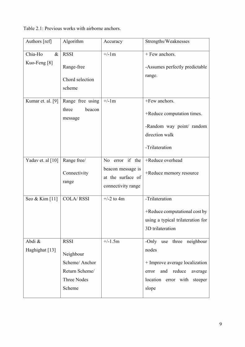
The previous 3D localization work from airborne anchors focussed on range-free 3D localization.
There is less work concerned with the 3D localization using a range-based algorithm for mobile
anchors, which should be able to provide substantially better accuracy. Table 2.1 lists the previous
work in the airborne mobile anchor area.
9
Table 2.1: Previous works with airborne anchors.
Authors [ref] Algorithm Accuracy Strengths/Weaknesses
Chia-Ho &
Kuo-Feng [8]
RSSI
Range-free
Chord selection
scheme
+/-1m + Few anchors.
-Assumes perfectly predictable
range.
Kumar et. al. [9] Range free using
three beacon
message
+/-1m +Few anchors.
+Reduce computation times.
-Random way point/ random
direction walk
-Trilateration
Yadav et. al [10] Range free/
Connectivity
range
No error if the
beacon message is
at the surface of
connectivity range
+Reduce overhead
+Reduce memory resource
Seo & Kim [11] COLA/ RSSI +/-2 to 4m -Trilateration
+Reduce computational cost by
using a typical trilateration for
3D trilateration
Abdi &
Haghighat [13]
RSSI
Neighbour
Scheme/ Anchor
Return Scheme/
Three Nodes
Scheme
+/-1.5m -Only use three neighbour
nodes
+ Improve average localization
error and reduce average
location error with steeper
slope
10
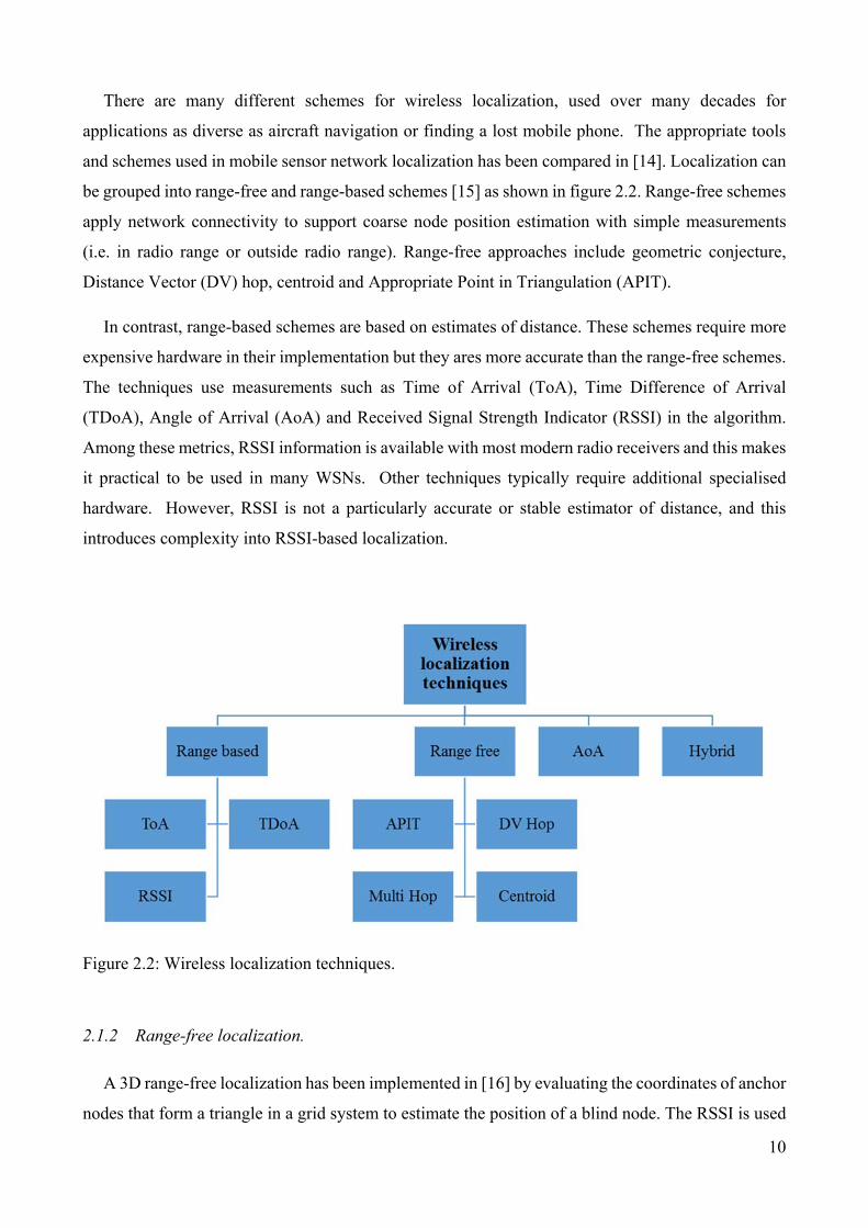
There are many different schemes for wireless localization, used over many decades for
applications as diverse as aircraft navigation or finding a lost mobile phone. The appropriate tools
and schemes used in mobile sensor network localization has been compared in [14]. Localization can
be grouped into range-free and range-based schemes [15] as shown in figure 2.2. Range-free schemes
apply network connectivity to support coarse node position estimation with simple measurements
(i.e. in radio range or outside radio range). Range-free approaches include geometric conjecture,
Distance Vector (DV) hop, centroid and Appropriate Point in Triangulation (APIT).
In contrast, range-based schemes are based on estimates of distance. These schemes require more
expensive hardware in their implementation but they ares more accurate than the range-free schemes.
The techniques use measurements such as Time of Arrival (ToA), Time Difference of Arrival
(TDoA), Angle of Arrival (AoA) and Received Signal Strength Indicator (RSSI) in the algorithm.
Among these metrics, RSSI information is available with most modern radio receivers and this makes
it practical to be used in many WSNs. Other techniques typically require additional specialised
hardware. However, RSSI is not a particularly accurate or stable estimator of distance, and this
introduces complexity into RSSI-based localization.
Figure 2.2: Wireless localization techniques.
2.1.2 Range-free localization.
A 3D range-free localization has been implemented in [16] by evaluating the coordinates of anchor
nodes that form a triangle in a grid system to estimate the position of a blind node. The RSSI is used
11
to compare with a threshold value in order to localize the blind node. The results show that the scheme
has less error if the anchor nodes are uniformly distributed during the deployment.
Blind nodes are localized using in 3D node range-free localization in [17]. Anchor nodes are
randomly distributed to localize the randomly distributed target node located at the middle and bottom
layer boundaries. The problem of non-linearity between RSSI and distance is solved by using a fuzzy
logic system. RSSI information between the two nodes is sufficient for the target nodes to estimate
its position. The location of the target node is computed based on the edge weights between the target
and neighbouring anchor nodes using a Fuzzy Logic System (FLS). The results have been compared
with other range-free algorithms such as Hybrid-Particle Swarm Optimisation (HPSO), centroid and
weighted centroid to show that this algorithm has better performance than the other algorithms.
From the viewpoint of cost and energy consumption, the range-free algorithm is preferable since
it does not require hardware to measure distance or angle. The mobile anchor node with GPS will
periodically broadcast a beacon message including its current location. The mobile anchor node is
assumed to move in a straight line. The initial work in [8] has been improved in [18] by obtaining
possible points through the intersection of three spheres. The position of blind nodes is determined
from these intersection points. As a results, the scheme provided higher localization accuracy
compared to Ou’s scheme in [8]. Additionally, more appropriate path planning is part of their future
investigation since the existing path results in poor localization accuracy.
A range-free algorithm called three-dimensional azimuthally defined area localization (3D-
ADAL), has been proposed in [19]. The estimated position of blind nodes is based on the information
received from the mobile anchor node that is equipped with a rotary and tilting directional antenna.
The algorithm has the advantages of being simple and produced higher energy efficiency that
contributes to the sensor’s lifetime. The sensor nodes within the ranges of the mobile anchor node
received a beacon messages that depends on the angular velocity of the directional antenna, the time
between each transmission and the velocity of the mobile anchor node. The error can be reduced by
increasing the number of virtual beacon nodes and by decreasing the beamwidth of the directional
antenna. The work needs to be improved in order to accomplish larger distance data communications
to the WSN.
Range-free localization is based on the radio connectivity between nodes and does not use a
distance measurement [20] to infer the location. It does not require any extra range estimation
hardware like range-based localization. However, it only provides coarse accuracy. Range-free
methods can be classified as centroid system, distance vector (DV), hop terrain, and appropriate point
in triangulation (APIT) [1], and these are described in more detail below.

12
2.1.2.1 Centroid system.
Bulusu and Heidemann [21] proposed a centroid algorithm that uses anchor beacons with location
information to estimate the blind node’s position. The multiple anchor nodes will broadcast their
positions from their GPS receiver to the blind nodes [22]. The blind node (Xest, Yest) estimates its
location using the average of all N beacon positions as follows:
, ⋯ , ⋯ (2.1)
2.1.2.2 Distance Vector (DV Hop).
A DV HOP [23] measures the number of hop counts from each blind node to anchor nodes using
the hop count techniques and triangulation. The hop count method is useful to find the hop between
the two nodes in isotropic networks. The distance between the hops can be determined using the
multiplication of the average per hop. For instance, the anchor will broadcast a beacon throughout
the network, which consists of the anchors location and a hop count parameter initialized to one. Each
blind node will maintain the minimum counter value per anchor of received beacons and it will ignore
those beacons with higher hop-count values. Thus, this mechanism will allow all nodes in the network
to get the shortest distance in hops to every anchor. Using the following formula, the average single
hop distance estimated by the anchor can be obtained.
(2.2)
Where, , is the location of anchor j while hj is the distance in hops from anchor j to anchor
i. Once the hop size is calculated, the anchors will propagate this information out to the nearby nodes.
Finally, the location of the blind nodes can be estimated using a multilateration algorithm.
In [24] the improved DV hop algorithm has been proposed to increase the accuracy and produce
lower computational complexity. The algorithm is enhanced by adding additional localization
information such as the direction of arrival.
2.1.2.3 Hop Terrain.
The hop terrain algorithm finds the distance between anchor and blind node as follows. The blind
node obtains its initial position estimation by using the DV hop algorithm above. Then the initial
position estimation is broadcast to the neighbour nodes. The neighbour nodes receive the information
that contains estimates of distance information. This algorithm minimizes the least square error
between inter-node distances based on the estimated positions and average of inter-hop distance. In
13
[25] the performance of Hop Terrain is analysed and they proved that the node is localized up to a
bounded error based on average hop distance.
2.1.2.4 Appropriate Point in Triangulation (APIT).
In the APIT scheme [26], the blind node connects to the anchor nodes to get the position
information of anchor nodes and the energy information of received signal energy. Using this
algorithm, it chooses 3 nodes among N anchor nodes to test whether the blind node is within the
triangle, formed by these 3 anchor nodes. If so, the position of the blind node is determined as the
centroid of this area.
The main drawback of APIT is it requires more anchor nodes than the average number of anchors
in localization [27]. Furthermore, it also does not make any assumption about the correlation between
absolute distance and the radio signal strength.
Overall, the range-free localization schemes require less information and simpler receivers than
range-based localization, however they are less precise. Given that RSSI is now available on almost
all WSN radio receivers, no extra complexity in hardware is required to achieve the better accuracy
of range-based techniques. The following sections explain these techniques.
2.1.3 Range-based algorithms.
Range-based localization techniques calculate the position of blind nodes through the estimation
of distances or angles from anchors, using techniques like triangulation, trilateration, or
multilateration. The system can use long-range anchors that transmit over the whole network or it use
a short-range beacon that transmits to a local subset of nodes.
The work in [28] discusses the various range-based techniques for localization by using the
distance or angle, by using the weighted RSSI, by using the geometry of beacons or by using
cooperative localization between blind nodes. The geometric arrangement of anchor nodes can be
used as a strategy to improve the accuracy. The equilateral triangle of mobile anchor node at proper
placement improved the position estimation compared to random placement [29] [30]. The localized
blind nodes can be used as new local anchors as in [31].
2.1.3.1 Ranging signals.
Audio and radio frequency signals are the common used for ranging. They differ in terms of speed,
wavelength and frequency. Radio signals travel at speed of light, approximately a million times faster
than audio signals at a few hundred metres per second in air.

14
The work in [32] presented the results from three different systems applied in 3D position
measurement. Two commercial systems are based on radio frequency measurements while the other
employs a time-of-flight measurements based on audible signals in an acoustic prototype system. The
experiments focused on the accuracies of the systems, the position update rates, the end-to-end delay
as well as the energy consumption. The tests were implemented for indoor localization with stationary
measurements at known positions, and with dynamics scenarios on a linear track at given velocities.
The Sound-Based Localization System (SBLS) performed well in terms of accuracy and precision of
the position. Its low update rate and high latency is suitable for stationary localization. One RF
system, Decawave, provided a very high update rate and low delay, making it suitable for the dynamic
applications. The other RF system, a Time Domain system, not only provided higher update rates but
also lower delay with better accuracy than the Decawave system. When comparing these three
systems in cluttered environments, (SBLS, Decawave and Time Domain), the reception of acoustic
signals was greatly disturbed by the obstructions thus it led to poor performance for SBLS. This
scenario can be dealt with in a better way by using the RF based systems. The following sub section
will discusses the most common range measurement techniques.
2.1.3.2 Time of Arrival (ToA).
This technique uses the propagation time between signal transmission and reception, plus the
transmission speed of the medium to estimate distance. This approach is commonly used for acoustic
ranging. However, the technique needs very high clock accuracy and time synchronization for use
with RF, and is not practical with WSN-grade technology [33].
In ToA, the time of emission can be included in the beacon and received by the time-synchronized
sensors [34], or it can be at known times. Once the features of the signal are obtained, ToA
measurements are compared to the transmission time. Here the beacon transmitted by the anchor
consists of the anchor positions and the time of transmission. Given a formula for ToA;
Time of Flight (ToF) = (time of reception - time of transmission) (2.3)
Therefore, the range estimate can be calculated using the following formula.
Range = ToF / Propagation speed (2.4)
2.1.3.3 Time Difference of Arrival (TDoA).
In TDoA, the unknown time of emission is eliminated by calculating the difference between
arrivals of one signal at two receivers. The blind node sends a message (at unknown time) and

15
synchronised anchors will record the arrival times to give TDOA. This requires very high
synchronization between transmitters (anchors) but does not requires transmitter-receiver
synchronization. It has been used in aircraft navigation, with expensive base stations. Localization
in TDoA (shown as the red curve) is referred as hyperbolic positioning whereby the emitter position
on a hyperboloid is localized with the two sensors as foci as shown in figure 2.3.
Figure 2.3: Multilateration using TDoA and ToA measurements with hyperbolae and circles
respectively as possible emitter location. Adapted with permission from [34].
The measurements of TDoA is obtained by calculating the difference between two ToA
measurements and the unknown time of emission will be eliminated. There should be a pair of sensors
to get the measurements.
The most common methods used for TDoA is the generalized cross correlation method. The cross
correlation function between two signals received from two receivers is given by integrating the lag
product of two received signals for a sufficient time period [35].
2.1.3.4 Received Signal Strength Indicator (RSSI).
Received Signal Strength Indicator (RSSI) is a measurement of the RF power received at the
receiver. Assuming known transmit power, receiver antenna gains, and signal path loss as a function
of distance, RSSI can be used to estimate transmit distance.
RSSI is calculated from the antenna voltage being measured at the receiver and is indicated as a
measured power. RSSI ranging calculates the propagation loss and transforms the value into the
distance, using an experimental or theoretical signal path loss model. The signal strength is influenced

16
by at least three environmental factors such as the node elevation from the ground, transmission
power while collecting the data and the position of the antenna [36].
In [37], the localization of the deployed blind nodes uses RSSI as a range estimation technique.
As suggested by the commonly used log-normal shadowing model for Radio Frequency (RF)
propagation, RSSI is a random variable based on distance. Therefore, the estimate of ranging distance
using RSSI is also a random variable. It is also known as an inaccurate distance estimator [6], and
errors in distance estimation are worse for larger distances. RSSI ranging is explored in detail in
Chapter 4.
2.1.4 RF propagation models, advantages and disadvantages.
Line Of Sight (LOS) is where the transmit and receive stations are in view of each other without
any sort of an obstacle between them. Point-to-point microwave links and satellite transmission are
examples of line-of-sight communication. RSSI measurements are sensitive to multipath, diffraction,
fading and non LOS measurement. RSSI is difficult to use as a range estimator in cluttered or indoor
environments.
RSSI can be modelled with a Free Space propagation model, Two-Ray ground model, and with a
Log Normal Shadowing Model (LNMS). Among these categories, LNMS is the most common signal
propagation model and does not have any special requirements for the application environment [38].
a) Free space propagation model.
This model is used when the transmitter and receiver have clear LOS between them, thus the RSS
can be predicted and is given by the Friss free equation.
Pr (d) = (Pt . Gt . Gr . 2) / (4 )2 . d2 . L (2.5)
where Pt is transmitted power, Pr (d) is received power, Gt is transmitter antenna gain, Gr is the
receiver antenna gain, D is the transmitter to receiver separation distance (m), L is system loss factor
and is the wavelength in metres. For a given transmitter and receiver configuration, Pt ,Gt ,Gr, and
are all constant, so the relationship can be more easily be seen.
b) Two-ray ground model.
This model considers the path between the transmitter and receiver consists of two rays: the direct
ray and a ground reflected ray. The two rays destructively interfere (reflected ray is opposite in phase
after reflection) and as distance (d) increases the relative phase difference decreases between LOS
and reflected wave. Thus, the attenuation is more rapid than the free-space model.

17
Pr (d) = (Pt . Gt . Gr . (ht2 hr
2)) / d4 (2.6)
where ht is the transmitter antenna height and hr is the receiver antenna height.
c) Log Normal Shadowing Model.
Since RSSI measurement is readily available, it has become a popular topic in localization
research. Its unpredictable performance can be considered as being due to Gaussian noise, and this
fits with the existing log normal shadowing model for noisy communication paths.
The major variability of RSSI is due to extrinsic and intrinsic factors, i.e. factors about the
environment and factors about the device. In extrinsic factors, error is caused by the properties of the
wireless channel, for example fading, interference and obstructions. In random fading, the multipath
and shadowing effects are two major sources of error. In multipath, the signal contains error because
of reflection, diffraction and dispersion. Interference and additive noise cause a random variation of
RSSI and this interference noise is not stationary. Another major error is caused by intrinsic factors
in the radio platform. The behaviour of the transmitter and receiver electronics contribute
measurement noise, e.g. not all receivers will transmit at exactly their nominal power.
LNSM is a general propagation model which is suitable for many different environments. The path
loss (PL) can be calculated as;
PL (db) = PL (d0) + 10 . n . (log d/d0) + Xσ (2.7)
where d0 is the reference distance used for the experimental measurement PL(d0), n is the path loss
index (depends on environment, typically between 2 and 4), σ is the zero mean Gaussian variable and
X is the standard deviation of the variability.
2.1.4.1 Probability distribution using Log normal shadowing model.
A relationship between RSSI and distance is best described through the Log Normal Shadowing
Model (LNSM). It is chosen as the preferred RSSI signal propagation model since it is a general
parameterisable signal model as compared to the free space model and 2-ray ground model. The other
two models however have special requirements for the application environment such as the
transmission distance should be larger than the antenna size and the carrier wavelength and there
should not be any obstacle in between the transmitter and receiver. Also, they are deterministic
formulas and do not capture the noisy nature of RSSI measurements. LNSM is suitable for indoor
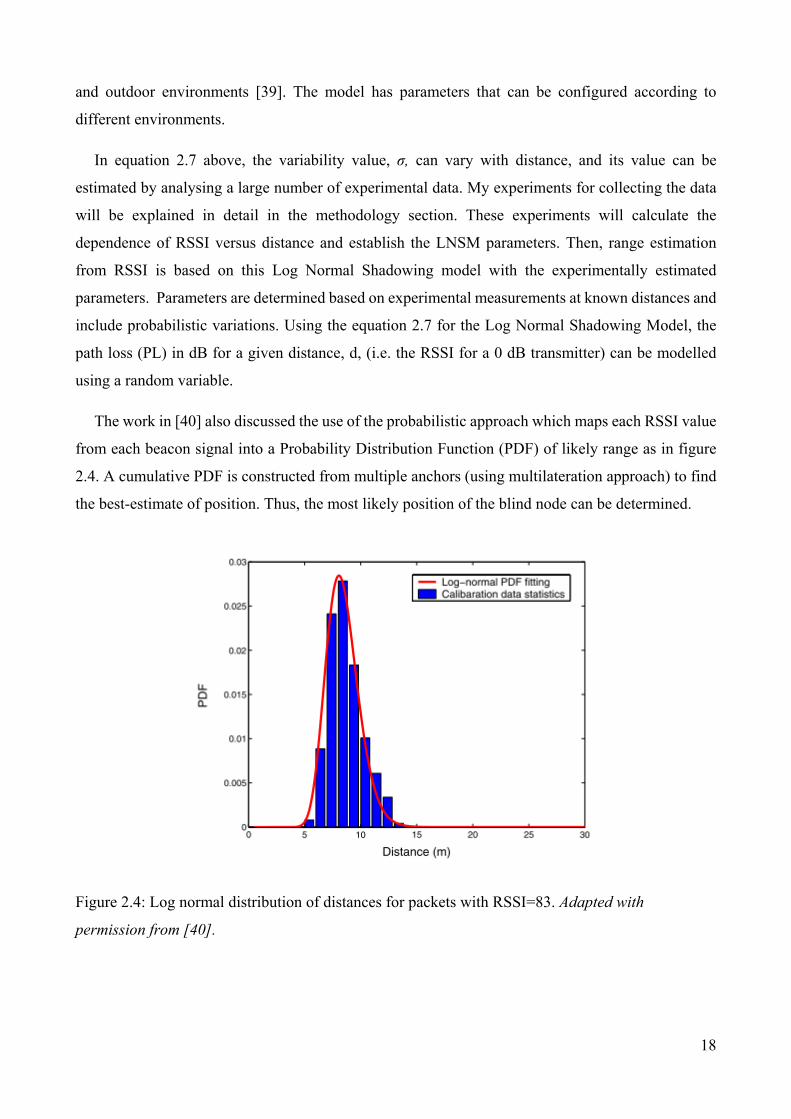
18
and outdoor environments [39]. The model has parameters that can be configured according to
different environments.
In equation 2.7 above, the variability value, σ, can vary with distance, and its value can be
estimated by analysing a large number of experimental data. My experiments for collecting the data
will be explained in detail in the methodology section. These experiments will calculate the
dependence of RSSI versus distance and establish the LNSM parameters. Then, range estimation
from RSSI is based on this Log Normal Shadowing model with the experimentally estimated
parameters. Parameters are determined based on experimental measurements at known distances and
include probabilistic variations. Using the equation 2.7 for the Log Normal Shadowing Model, the
path loss (PL) in dB for a given distance, d, (i.e. the RSSI for a 0 dB transmitter) can be modelled
using a random variable.
The work in [40] also discussed the use of the probabilistic approach which maps each RSSI value
from each beacon signal into a Probability Distribution Function (PDF) of likely range as in figure
2.4. A cumulative PDF is constructed from multiple anchors (using multilateration approach) to find
the best-estimate of position. Thus, the most likely position of the blind node can be determined.
Figure 2.4: Log normal distribution of distances for packets with RSSI=83. Adapted with
permission from [40].
19
2.1.4.2 RSSI and its relationship to distance.
In practice, RSSI is influenced by many environmental factors such as the node elevation from the
ground, transmission antenna pattern, multipath, obstructions, interference and the position of the
antenna [36]. RSSI is chosen as a common technique to estimate the distance between two sensor
nodes. It has been used as a range estimator in many indoor and outdoor applications, such as in [41]
and [37].
RSSI based distance estimation for localization using only 3 anchor nodes is implemented in [42].
This work, which is based on geometrical computation, analysed the energy and communication cost
in localization process. It also introduced the use of virtual anchors instead of using only 3 anchors
in the trilateration algorithm. Internode localization is applied after all blind nodes were able to
determine their approximate location using anchors and virtual anchors. This algorithm reduced the
error propagation by collaboration among nodes. Using a limited number of actual nodes it can
produce more anchors which are the combination of actual and virtual anchors. The nodes without
three non-collinear nodes suffered from flip ambiguity issues producing higher error. However, this
problem can be further reduced using nodes with higher density. The results show that the maximum
error is less than 4 metres. Their analysis is a useful input to my research in determining the minimum
number of anchors to use.
An empirical study to investigate the localization accuracy among a wide selection of range-based
localization scheme using radio signal strength measurement has been conducted in 2 different
environments, viz. an empty corridor and a research lab in [43]. They investigated the number of
anchor nodes needed to reduce the localization error and analysed the performance of different
algorithms. They concluded that RSSI based localization did not provide an accurate localization in
indoor localization by using only a limited number of beacons deployed in that area. Their work has
been further enhanced by [44] by employing a new RSSI-based tracking system. It exploited a priori
knowledge about the system setting and it derived a lower bound of possible performance based on
the Cramer Rao Lower Bound (CRLB) that is tailored to the path shape using the static channel
conditions. They conducted a series of experiments for sensors tracking on various paths using two
anchor nodes. Extension of the tracking system to a 3D environment is planned to be carried out in
their future work. Again, using only two anchor nodes is not preferable in my research since I am
looking at the impact of number of anchors on the localization error.
The algorithm in [45] is currently being implemented in 2D but it is extendable to 3D space. The
authors introduced a minimalistic algorithm called Relaid Ranging Localization (ReNLoc) that used
a multilateration algorithm with centralized networks. It takes the geometric constraints that arise

20
from the range measurements into consideration. Future work will consider a distributed version of
the system.
A typical experiment that can be performed in indoor and outdoor environments using WSN nodes
for determining a model of distance versus RSSI is described in [46]. This method selects appropriate
values of LNSM parameters (PL(d0), n) to give the best fit to experimental data. This model gives a
deterministic value for d given the RSSI.
Hence, given an RSSI path loss, PL(dx) at unknown distance, dx can be estimated as:
dx = 10 * [((PL (dx) - PL (d0)) / (10.n)] (2.8)
Overall from the above discussion, among these three techniques (ToA, TDoA and RSSI), RSSI
based localization algorithm is chosen since it is the most practical and applicable in our research.
2.2 Angle of Arrival (AoA).
Angle of Arrival (AoA) has been a popular research topic even though the algorithm is rarely
considered for WSNs since it requires a large array of directional antennas. Yet, it can still be suitable
for small sized sensor nodes as in [47]. In this algorithm, the sensors nodes will forward their bearings
with respect to the anchors. The antenna of the anchor node used to find the direction to the blind
nodes. The beacons are transmitted by an antenna that rotates at constant angular speed and schedule.
The sensors determine when the power of the beacon is at its strongest and hence the angle to the
anchor.
Triangulation is a common method to compute the node’s position based on the information of the
angles instead of distances. The measurements are taken from at least three anchor nodes. Therefore,
the blind nodes will be able to compute their own location using simple trigonometrical relationships.
Triangulation is used to improve the location accuracy using the information from the cluster head
(anchor node) and the angle to the anchor node from the blind nodes in [48]. However, using the AoA
algorithm alone can result in high cost because it involves many complex signal sources and precise
clock synchronization. A hybrid system combines ranging estimates with AoA measurements and
may be a better alternative, as described in the next section.
2.2.1 Angle with range-based localization (Hybrid system).
The authors in [49] and [50] investigate the localization in a 3D WSN using a hybrid system that
fuses distance from RSSI and AoA measurements. A novel objective function using a least square
(LS) criterion is derived. The method is used for two different cases, non-cooperative and cooperative

21
localization. For non-cooperative localization, they proposed two novel estimators that able to reduce
the estimation error. While for cooperative localization, they presented the hybrid system using RSSI
and AoA for estimating the target or blind node. The RSSI distance estimate is obtained through the
path loss model while the angle measurement in term of azimuth and elevation angle is assumed to
be obtained from either multiple antennas or a directional antenna at the anchor. Here, the digital
compass determines the orientation information of different sensors. Unfortunately, the measurement
error due to the compass’s static accuracy will occur. Therefore, they model the angle measurement
error and the orientation error as random variables. Generally, the hybrid system for both non
cooperative and cooperative localization are an improvement compared to earlier results in [51]. The
LS and maximum likelihood algorithm (ML) that combines both RSSI and AoA measurements is
implemented to estimate the target position. In [52], they proposed using only the two best RSSI
measurements from anchors for intra-cell localization. However, in this work, only non-cooperative
localization for 2D scenario are investigated.
Another hybrid approach that benefit from RSS and AoA measurement has been proposed in [53].
The algorithm implemented the multi-step Gaussian filtering approach instead of using the initial
hybrid method with a particle filter. This is due to the multi modal or non-Gaussian nature in non-
line of sight (NLOS) propagation. The algorithm also used a Kalman filter approach. The first step
of the filtering process used RSSI input to determine the linearization point. Then both RSSI and AoA
inputs used in the second steps of filtering. Thus, the filtering process could eliminate the effect of
uncertainty in propagation parameters. Here, the altitude of the RF source is not estimated and the
UAV is assumed to fly at certain altitude in a circular path. The distance of RSSI and AoA
measurement are set to be 20km. Using a hybrid system allows localization using a single anchor in
2D, or in 3D if bearing and azimuth angles are calculated.
In our research, we will be assuming simple WSN nodes, and so we do not plan to use AoA in our
algorithms.
2.3 Implementation of GPS-based localization on mobile anchor node.
GPS positioning uses a type of multilateration based on time of arrival from satellites at known
coordinates plus estimates of path propagation speeds. A detailed explanation is given in [54]. Each
packet is time stamped with accurate time and position information, based on on-board atomic clocks
on the satellites. For point positioning, GPS requires four (4) pseudo ranges to four satellites, solving
for four unknowns (x, y, z position and receiver clock offset).

22
GPS accuracy is affected by several factors such as the satellite positions, noise in the radio signal,
natural barriers to the signal as well as due to the atmospheric conditions. An error, which is typically
between 1 to 10 metres, is created by noise from the interference, and this can be up to 30 metres for
interference from large objects such as mountains. An accurate position can be obtained in the case
of a clear line of sight and the accuracy can be increased with the help of other technologies such as
Differential GPS (DGPS) and Assisted GPS (AGPS). DGPS is used in [55] to enhance the
localization accuracy and this helps a mobile robot to estimate its position with a small uncertainty
of less than 3 metres. A single GPS can be combined with DGPS for correcting the mobile robot’s
position which has been estimated by the optical navigation sensor and Inertial Measurement Unit
(IMU). However, DGPS needs high quality communication between the robot and the base station.
AGPS uses additional information from other radio sources to improve GPS localization. In [58]
AGPS readings are used to recalibrate a mobile phone location periodically, and this location can be
used as a references for further position estimation [56] .
Even though GPS is a powerful tool for localization, it is often impractical to equip each WSN
node with a GPS device due to the cost. Also, the GPS signal is often weak and unavailable in many
environments such as indoors and in forested zones.
For our research, GPS will be used only on a single mobile anchor node. It is impractical to provide
GPS on each of the blind sensor nodes. GPS is used to define the accurate position of the mobile
anchor node at certain points while travelling in the sensing area. This information will be sent
through a beacon packet by the mobile anchor node to all blind nodes within its range. Once the blind
node receives the beacon packets and their associated RSSI from several anchor points, the estimated
position of the blind node can be determined.
2.4 Multilateration algorithm for localization.
Localization of nodes with range-based techniques involves estimating the distance between a
transmitter and receiver by using features of the transmitted signal such as Radio Signal Strength
Indicator (RSSI) as described in the previous section. Then, the estimated distance is use to determine
the position of the blind nodes using an appropriate localization technique such as multilateration.
Multilateration can be implemented in 2D by intersecting at least 3 circles (trilateration), and in 3D
space by intersecting a minimum of four spheres centred on four anchors. For more than the minimum
number of spheres, multilateration provides a least squares error solution, and so more anchors can
improve accuracy. However, it is necessary to identify the appropriate number of anchors that are
able to reduce the localization error without excessive computation.

23
Multilateration as defined in [17], [45] and [57] is an extension of trilateration [58] and more
anchors are used to reduce the influence of distance error in localization. The algorithm determines
the position of the blind node, which is located at the intersection point of the spheres centred on the
anchors as shown in figure 2.5 where A1 to A5 are anchors with known position while B is the blind
node.
Figure 2.5: Intersection points of spheres in Multilateration.
The spheres as in the above figure can be described as;
(x-xi)2 + (y-yi)2
+ (z-zi)2 = di
2 (i=1,2,…nR) (2.9)
where, x y and z are the position of the blind node, while xi , yi, zi ,are the positions of anchor nodes
numbered from 1 to nR., and di is the distance between blind node and anchor i. The next section
shows how estimates of di are used to calculate x, y, z.
2.4.1 Deterministic and Probabilistic Multilateration.
Localization techniques can use either deterministic or probabilistic methods to determine the
positions of blind nodes. Deterministic localization provides a simple algorithm with acceptable
performance. The range for a specific RSSI reading is taken as the most likely value based on previous
calibration experiments. Probabilistic techniques use more information from the spread of range vs
RSSI measurements. For example, ranges with higher errors are given less weight in the calculation
of the solution. Despite the fact that probabilistic localization offers superior performance, the
computational complexity is a challenge as it requires a higher number of RSSI samples taken per
position in the calibration phase [59]. Thus it affects the training time and cost. In probabilistic

24
methods, a Bayesian decision process is used to estimate the most likely position of blind nodes in
the sensing area.
The authors in [60] discussed the use of the probabilistic approach to restrict the possible location
of the nodes by mapping each RSSI from each beacon signal into a Probability Distribution Function
(PDF). PDFs from all beacons are combined into a single PDF, and the most likely position of the
blind node can be determined.
This work was further enhanced in [41] which determined the position of blind nodes with
inaccurate range using multiple and sparsely located mobile nodes. Location refinement is based on
iterative and collaborative efforts. They concluded that the probabilistic model is suitable for outdoor
environments and it performed well compared to the proximity (range-free) measurement.
However, based on existing research and also the comparisons of probabilistic and deterministic
approaches [61], no prior work has examined how many RSSI measurements are needed for accurate
localization, especially using a probabilistic method used for outdoor application.
For our research, we will examine both deterministic multilateration and probabilistic
multilateration. The detailed mathematical equations used for deterministic and probabilistic
multilateration will be discussed in detail in chapter 4.
2.5 Gradient descent solution of multilateration.
Gradient descent is an iterative optimization algorithm to find a local minimum of a convex
function [40]. For multilateration, gradient descent is used as optimisation technique to find the best
estimate of location. Tools and techniques used in mobile sensor network localization are described
in detail in [14] and [61] including Gradient Descent and Multilateration algorithms.
Gradient descent optimization for solving multilateration is described in [62]. This algorithm
reduced the effect of inconsistent measurements to achieve a good localization accuracy and
computational efficiency. Based on MATLAB simulations, the authors showed that the gradient
descent algorithm performs better than the voting based scheme and Least Median Square based on
computational time and memory complexity. They concluded that the computational complexity
increases linearly with the number of iterations and the proposed method has better localization
accuracy compared to the other methods.
The work in [63] proposed a modification in the system using gradient descent to localize the node
with low computational complexity and better convergence performance. The gradient descent
method (GDM) suffers from low speed of convergence. Thus, the modification in this work is to

25
increase the speed of convergence by optimising the step size at each iteration. A Monte Carlo
simulation was performed for 100 x 100m region by using 100 random distributed anchor nodes to
localize an array of blind nodes uniformly spaced by 2m from each other. The average is taken from
100 iterations of multilateration calculations performed by all blind nodes. The distances between
nodes is estimated by RSSI and typically assumes as a Gaussian distribution. The estimated starting
position of the blind node is chosen as the geometrical centre of the three closest anchor nodes. The
results show that the algorithm improved the existing scheme while providing less computational
resources.
In [64], gradient descent optimisation is used for 3D localization in WSNs and was combined with
an iterative push-sum (PS) gossip based algorithm. Four anchors are needed and additive Gaussian
noise for measurement errors are modelled. However, the ToA distance measurement technique is
applied.
Modern mathematical toolboxes such as MATLAB provide efficient, customizable Gradient
Descent optimization solvers, and these will be used extensively in our later experiments.
2.6 Beacon geometric sensitivity and its placement.
Multilateration is known to be significantly affected by anchor geometry. For mobile anchors, the
position of beacons depend on the flight path, and the spacing of beacon messages in that path. There
are limited studies on mobile anchor placement since more attention has been given to localization
accuracy and computational effort.
Guidelines to optimize the beacon placement by considering the ratio between the distance and the
radio range, and the minimum height of the triangle formed by the anchors and the blind node is
proposed in [65]. The impact of anchor node placement and its rules as well as using the smallest
number of anchor nodes are discussed. This work is in 2D scenario but it can be expanded to 3D
localization.
Some aspects of beacon positioning especially the effect of anchor node placement on the
localization errors on a network-wide basis is explored in [66]. This approach could minimize the
number of anchors required while avoiding poor locaization. Additionally, the cost can be minimized
if the network uses the minimum number of anchors located at the best position. They found that
estimated ranges at acute angles (less than 90 degrees between the ranging rays) gives good
localization. They proposed to place the anchors near the centre of the network area. Even though
this work looked at 2D Problems, it can provide a methodological approach for our 3D scenario.
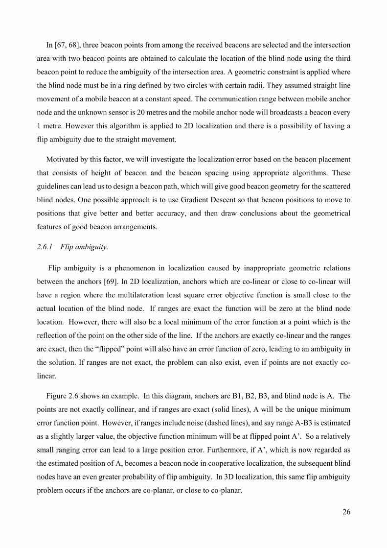
26
In [67, 68], three beacon points from among the received beacons are selected and the intersection
area with two beacon points are obtained to calculate the location of the blind node using the third
beacon point to reduce the ambiguity of the intersection area. A geometric constraint is applied where
the blind node must be in a ring defined by two circles with certain radii. They assumed straight line
movement of a mobile beacon at a constant speed. The communication range between mobile anchor
node and the unknown sensor is 20 metres and the mobile anchor node will broadcasts a beacon every
1 metre. However this algorithm is applied to 2D localization and there is a possibility of having a
flip ambiguity due to the straight movement.
Motivated by this factor, we will investigate the localization error based on the beacon placement
that consists of height of beacon and the beacon spacing using appropriate algorithms. These
guidelines can lead us to design a beacon path, which will give good beacon geometry for the scattered
blind nodes. One possible approach is to use Gradient Descent so that beacon positions to move to
positions that give better and better accuracy, and then draw conclusions about the geometrical
features of good beacon arrangements.
2.6.1 Flip ambiguity.
Flip ambiguity is a phenomenon in localization caused by inappropriate geometric relations
between the anchors [69]. In 2D localization, anchors which are co-linear or close to co-linear will
have a region where the multilateration least square error objective function is small close to the
actual location of the blind node. If ranges are exact the function will be zero at the blind node
location. However, there will also be a local minimum of the error function at a point which is the
reflection of the point on the other side of the line. If the anchors are exactly co-linear and the ranges
are exact, then the “flipped” point will also have an error function of zero, leading to an ambiguity in
the solution. If ranges are not exact, the problem can also exist, even if points are not exactly co-
linear.
Figure 2.6 shows an example. In this diagram, anchors are B1, B2, B3, and blind node is A. The
points are not exactly collinear, and if ranges are exact (solid lines), A will be the unique minimum
error function point. However, if ranges include noise (dashed lines), and say range A-B3 is estimated
as a slightly larger value, the objective function minimum will be at flipped point A’. So a relatively
small ranging error can lead to a large position error. Furthermore, if A’, which is now regarded as
the estimated position of A, becomes a beacon node in cooperative localization, the subsequent blind
nodes have an even greater probability of flip ambiguity. In 3D localization, this same flip ambiguity
problem occurs if the anchors are co-planar, or close to co-planar.

27
In [70], the analysis of flip ambiguity considered the ranging errors caused by the environmental
noise. They proposed an algorithm to detect and solve the flip ambiguity problem in various
situations. While their work is focused on the flip ambiguities in trilateration, it also can be extended
to a multilateration algorithm.
Flip ambiguity is a particular problem with airborne anchors, since a naïve flight path, which flies
over an area at a constant height is exactly the situation that can cause flip ambiguity. So later, in my
work on path planning, this problem will need to be considered.
Figure 2.6: Flip ambiguities. Adapted with permission from [70].
2.7 Indoor versus outdoor localization.
WSN localization is useful in both indoor and outdoor environments. The indoor localization
problem is more difficult than outdoor localization because GPS signals are not available within
buildings, and the RF signal propagation length estimation will be affected by signal interference and
signal reflections inside the building.
Outdoor localization can more easily use GPS to determine the position of the sensor. However,
unavailability of the GPS signal can be caused by the obstacles such as trees and buildings. Outdoor
localization of mobile sensors can use other techniques to improve accuracy such as odometry and
Interial Measurement Units (IMU). The work in [55] described an IMU solution combined with
odometry and GPS to overcome such problems. Such an approach is able to maintain tracking
stability even under severe conditions such as interruption of GPS signal and uneven ground surfaces.
Other approaches, such as the work in [71] use a unique RF attenuation model to cover the whole
area of interest.

28
Many experiments have been conducted for indoor and outdoor localization such as in [38], [72]
and [73] based on the signal strength from anchors. The area is divided into several subzones since
the receiving strength cannot be directly transformed into distance due to obstacles and multipath
within the building. While for outdoor environments, the scheme adopted the estimated distance to
determine the most likely position of the sensor node. As a result, the accuracy is improved for both
indoor and outdoor environments.
Another alternative technique for outdoor localization has been suggested in [56]. This approach
is to overcome the drawbacks of GPS of high energy use and unavailability in occluded environments.
Instead of using GPS as a preferred mode for outdoor localization, the techniques use the
accelerometer, microphone, compass and daily patterns of usage to gather the data and to identify the
sensor signatures for locating the devices. The signature or “fingerprint” localization improves
accuracy, device detection and battery usage. The aims of the research is to use a smartphone
equipped with camera and low power sensors to gather the information about the surroundings to
track daily activities, The system is a trade-off between accuracy and energy efficiency.
In fingerprinting based localization, the sensor signatures are matched against a previously
recorded geotagged database of signatures. The in-built sensors in a mobile device record the
signatures and detect the activity patterns. The sound signature of places can be recorded using the
microphone, while the Wireless Fidelity (WiFi) access points can also be used to detect the user’s
daily movement pattern. RSSI-based fingerprint based localization determines the location of the
mobile devices by matching the received signal fingerprint from different sources against the database
of known signal location information that has been previously recorded. The signal pattern can be
generated through the observation of RSSI values of different WiFi access points on a mobile device.
However, the database of signal fingerprints need to be constructed in advance, and it not always
stable.

29
Figure 2.7: Signal fingerprinting work by collecting the RSSI values from multiple WiFi access points
or base stations to generate a unique signature of an area. Adapted with permission from[56].
Fingerprinting involves two phases: the signal fingerprint populating phase (training phase) and
signal fingerprint matching phase (online phase). In the first phase, the signal fingerprint at each of
reference location will be recorded, therefore, the signal map can be generated. While in the second
phase, the signal fingerprint generated by the device will be compared with the pre-defined database,
and so the location of the mobile device can be estimated.
This technique is not directly applicable to our work since it requires a dense infrastructure of
access points or anchors, and also requires a dense mapping of the possible location area. However,
this method is useful for other indoor and outdoor applications such as in urban area with the
availability of WiFi access points.
A summary of many different fingerprinting studies is provided in [58], which shows the accuracy
of different fingerprinting methods by authors in different environments: visual (40-50m accuracy),
motion (5-10 m), radio such as WiFi and GSM (5-100m) and hybrid approaches (8-40m).
2.8 Centralized and distributed computation.
Localization schemes can be characterized into centralized and distributed algorithms.
In centralized computation, the data is obtained from the ranging phase and sent to a single central
server station. Once the data has been processed, the result will be transmitted back to the respective
nodes. A calibrated centralized localization technique using RSSI was earlier implemented in [71] for

30
outdoor environments. They presented a multihop localization technique by exploiting acquired RSSI
using a centralized approach. The attenuation model of the radio signal was build using Gaussian disk
model. Centralized localization can be energy inefficient for the sensor networks. It requires extensive
packet generation and the need of forwarding a lot of information to the central server. The data
transmission will cause latency and frequent localization for mobile nodes requires more consumption
of energy and bandwidth for communications, and requires a reliable communications path to the
server. The big advantages of centralized localization are that computation can be much more
complex than is possible on small WSN nodes, and the computation can use all information from all
nodes [74].
In distributed computation, the calculation is performed by each node based on its received
packets. This approach has better robustness against link or node failure, making this approach
suitable for many applications. It also offers higher scalability and independence in network structure.
The sensor nodes operate in a decentralized manner. However, the algorithms are more difficult to
design since local optimization may not perform well in a global sense. Additionally, for cooperative
localization, it requires multiple iterations to reach a stable solution resulting in a longer processing
time [35]. Another drawback of distributed localization is the energy consumption for computation
on the blind nodes [75]. The relative cost of communication versus computation, which may favour
distributed versus centralized computation will depend on the exact deployment scenario.
Because the choice of algorithm depends on variables such as computation cost and
communication cost, my research takes a middle road between these choices. The position of each
blind node is determined using only information received by each sensor node, so the algorithms
calculate the position of each node in an independent, distributed fashion. However, the focus of this
work is to investigate relatively complex algorithms, such as gradient descent optimization of
complex joint PDF models, and these calculations are computationally intensive. Currently, such
computations would be infeasible on small sensor nodes, so the algorithms are better implemented
on a centralized server. As technology advances, and energy efficient 32-bit processors with floating-
point arithmetic support become more common in sensor-grade nodes, my approach could also be
implemented as a distributed algorithm.
2.9 Static anchor node versus mobile anchor node.
Outdoor localization in a static WSN typically uses several static anchor nodes with known
positions to assist the localization of the blind nodes. These static anchor nodes that self-locate using

31
GPS typically are more expensive, and this contributes to higher system cost [76]. Often the self-
localizing feature of the static anchor node is not required after all blind nodes have been localized.
As alternative to the static anchor node is to use a self-localizing mobile anchor node which can
move through the deployment space and provide many anchor positions during localization, and
which can then be reused elsewhere afterwards. The mobile anchor node can be carried by either a
person on foot, an animal or a vehicle. In a sensor system, any transportation modality can be used
including utility aerial vehicle (UAV), utility ground vehicle (UGV) and multirobot system (MRS).
Furthermore, air dropped sensors which then use mobile anchor nodes used for outdoor localization
is one alternative to replace the traditional methods of hand placing sensors at known locations,
especially in the case of a large number of sensor or in a remote area.
A mobile anchor node is used to fully localize networks therefore it should needs sufficient energy
and capacity for a longer transmission range [77]. Since the energy efficiency of the mobile anchor
node is one of the main factor for the system, therefore, proper path planning is required to reduce
the energy consumption. This approach needs to identify the candidate area that guarantees a
reception of beacon messages. The proposed planning scheme reduces the movement distance and
the number of beacon messages of mobile anchor node and so it also minimizes the energy
consumption of the mobile anchor node.
Another problem that can be solved by using a mobile sensor is to avoid the obstructions that
occlude line of sight connectivity, and so prevent the nodes from obtaining the pairwise distances
between each other [78]. This work has another advantage that overcomes the sparse node
deployment with inadequate neighbours that necessary to obtain a unique solution. The geometric
dilution of precision (GDOP) that contributes large errors in its estimated position due to the longer
distance from a group could also be avoided.
In a static WSN, positions of blind nodes remain unchanged after the deployment of the nodes.
The position of the node is determined during the system initialization and fixed network routing
schemes can be implemented. If some or all of the nodes are mobile, then localization needs to occur
continuously, and is more complex [8]. In my research, the blind nodes are considered stationary,
except for a mobile anchor node that is moving during initialization.
Blind nodes can be localized using only one mobile anchor node, however the process can be
done more quickly with more mobile anchors such as in [79] and [80] which use between 1 to 8
mobile anchor nodes. The localization approaches addressed in this thesis will work equally well with
one or more mobile anchors.

32
2.10 Path planning for the mobile anchor node.
An important issue in using mobile anchor nodes will be what path the mobile anchor node should
follow, when and where it should transmit beacon packets. More beacon packets can potentially
improve localization accuracy, but it will have effects on the time and energy needed for localization.
Path planning may be pre-planned, or it may react to information from blind-nodes (e.g. some node
may indicate they have insufficient packets for accurate positioning, so the mobile anchor node may
change its path to accommodate these nodes).
The algorithm for anchor placement can be categorized as random, statically planned or
dynamically planned trajectories [81]. Poorly planned trajectories may cause a large localization
delay, low localization ratio and increase the localization error.
2.10.1 Random trajectories.
Mobile anchor node trajectory is discussed in [82], in which the researcher proposed a distributed
range-free localization scheme using a mobile anchor which moves randomly. Random paths can be
useful when the mobile anchor is carried by an uncontrolled host, such as by vehicles that happen to
be passing through the sensor area (such as a ship or an aircraft), or by an animal that is wandering
around in an area. However random paths do not guarantee good coverage, and are not used in my
thesis.
2.10.2 Dynamic trajectories.
The dynamic trajectories are not fully planned in advance and start with general information about
the sensing area such as the distribution of nodes, region of interest and nodes density. The anchor
will use all of this information while moving. The work in [83] implemented a dynamic path using
an algorithm called Deterministic beAcon Mobility Scheduling (DREAMS).
Such an approach involves a significant message overhead between anchor and blind nodes and
can take a long time since it is impossible to predict the anchor’s moving time and the path distance
in advance. Therefore, it will not be implemented in my research.
2.10.3 Static trajectories.
The statically planned trajectory is a well-planned path designed which should provide non-
coplanar anchor positions to avoid the flip ambiguity issues. The localization using a static trajectory
is further discussed in [55]. However, most of the positioning schemes are based on a range-free
approach that is not part of our research.

33
Static path planning schemes such as those in [84] and [85] consider factors such as the mobile
anchor node movement strategy, number of mobile anchor nodes and number of transmitted message
for localization. The work in [86] and [87] specifically discussed the comparison between choices of
trajectory pattern such as DOUBLE SCAN, HILBERTS, S-CURVES/ SPIRAL, and CIRCLES as
shown in figure 2.8. The requirements were that within a fixed path length, every possible sensor
point could see sufficient beacons within a maximum radio range (or chord length). It was concluded
that SCAN cannot guarantee the length of a chord doesn’t exceed a certain threshold, the beacon
overhead is higher in using DOUBLE SCAN, and three or more beacon points are required to
construct two chords for localization but this cannot be guaranteed by HILBERT. CIRCLES perform
worst for a square sensing region, leaving the four corners uncovered but it works well in a circular
sensing region and it has shorter path length compared to other schemes. While S-CURVES or
SPIRAL still need to have further enhancement since it also cannot guarantee that sensor nodes are
able to construct two valid chords.
Figure 2.8: Static path planning for (a) Scan (b) Hilbert (c) Circle and (d) S-Curves with individual
path length. Adapted with permission from [87].
Trajectory planning for trilateration also has been discussed by in [77] and they proposed the
algorithm of MoBile anchor node Assisted Localization (MBAL) to minimise the length of the
movement path for energy saving. For those nodes within insufficient beacons, additional messages

34
from the mobile anchor node will be requested, thus the path could be changed. In [88], the work
quantified the influence of mobile trajectory on localization error. They proposed a Localization
algorithm with a Mobile Anchor node based on Trilateration (LMAT) using an equilateral triangle of
beacon positions to overcome the problem of exact beacon location. Most of the proposed solutions
gave ideas on choosing the best trajectory for reducing the energy consumption and producing higher
coverage.
The author in [30] discussed how the localization performance would be influenced by these
criteria:
a) Communication range: the mobile anchor nodes should have a larger communication ranges thus
more blind nodes could be localized.
b) Movement trajectory: the flip ambiguity that caused by a collinearity problem can be eliminated
using a well-designed trajectory.
c) Broadcast interval: a shorter broadcast interval is preferred to enable the anchor broadcast its
location frequently.
d) Path length: a mobile anchor node has an opportunity to broadcast and pass by more blind nodes
if it has longer path length.
They introduced a new approach called Mobile Anchor Assisted Localization Algorithm based
on Regular Hexagon (MAALRH) with additional improvement using a boundary compensate method
(BCM) to assist with the four uncovered corners of the region. The 2D sensing region will be divided
into sub rectangles with the communication ranges of mobile anchor nodes being equal to the
resolution. The mobile anchor node is traversed by following the regular hexagon movement
trajectory. The estimated position of the blind node is calculated based on deterministic trilateration.
The performance of this algorithm is compared with HILBERT, SCAN, DOUBLE SCAN and
CIRCLES by varying the resolution in order to calculate the path length. Then the performance again
is compared based on the localization ratio, localization accuracy, path length and the scalability.
The optimal mobile anchor node path for best localization is still an open question. This thesis will
investigate the localization performance of some typical paths in terms of the accuracy versus number
of beacon positions taking account of geometric sensitivity. The deployment of anchors needs a
planned arrangement than a random deployment to ensure uniform coverage and sufficient accuracy
in localization, so different beacon path topologies will be investigated.
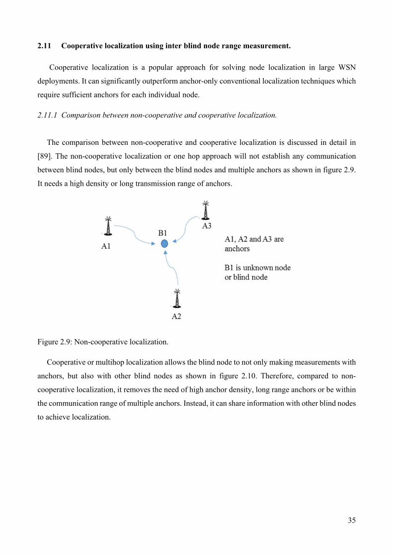
35
2.11 Cooperative localization using inter blind node range measurement.
Cooperative localization is a popular approach for solving node localization in large WSN
deployments. It can significantly outperform anchor-only conventional localization techniques which
require sufficient anchors for each individual node.
2.11.1 Comparison between non-cooperative and cooperative localization.
The comparison between non-cooperative and cooperative localization is discussed in detail in
[89]. The non-cooperative localization or one hop approach will not establish any communication
between blind nodes, but only between the blind nodes and multiple anchors as shown in figure 2.9.
It needs a high density or long transmission range of anchors.
Figure 2.9: Non-cooperative localization.
Cooperative or multihop localization allows the blind node to not only making measurements with
anchors, but also with other blind nodes as shown in figure 2.10. Therefore, compared to non-
cooperative localization, it removes the need of high anchor density, long range anchors or be within
the communication range of multiple anchors. Instead, it can share information with other blind nodes
to achieve localization.

36
Figure 2.10: Cooperative localization.
2.11.2 Implementation of cooperative localization.
In [90], a distributed approach with iterative multilateration has been proposed for cooperative
localization. Once the blind nodes establish their estimated position, they become anchors. A new
anchor will broadcast its estimated position to other neighbouring nodes. This is an iterative process
until all blind nodes can be localized using at least three reference nodes. The advantage of this
implementation is to reduce the communication cost since this repeating process only involves the
local neighbourhood. Unfortunately, one drawback is it suffers from the error propagation. These new
anchors inherit the estimation error produced from the first round of the localization process. Thus,
these errors are propagated to other nodes and errors get amplified. Accumulating errors may render
results useless if there are excessive iterations in the algorithm.
The author in [92] proposed a mechanism for choosing the reference nodes carefully by
considering the topology so that the accumulated error could be reduced. Due to the error propagation
problem from the erroneous estimates of the new anchors or virtual anchors that receives information
from multiple beacons, it contains of a degree of uncertainty in their estimation. Thus, the research in
[92] is focused on determining which combination of the references could produce the best
performance. The algorithm started with choosing an appropriate utility function to determine how

37
useful a node is for cooperative localization. The best nodes maximize the accuracy subject to
constraints given by the node’s limited processing capacity. The parameters used are number of
reference node, their uncertainty for virtual anchors, quality of range estimates and geometry. The
selection procedure starts by performing an exhaustive search. It will evaluates the combination
(coalition value) for sets of anchors, and then the set with the largest coalition value will be chosen.
However, this process leads to the exponential search time since the number of combinations is very
large. They considered a low density scenario with a small number of candidate nodes and so can use
an exhaustive search. The paper concluded that higher coalition values lead to more accurate position
estimates with improvement between 39% to 51% with respect to closest distance and random choices
for anchors.
Inter-node range-based measurement for the location estimation is used in [91]. The optimization
problem of determining the blind node’s position is formulated such that it will be consistent with the
inter node range measurement and the anchor node’s position. Localization using cooperative
localization also has been discussed in [92]. The author proposed a probabilistic, constraint-based
approach robust to range measurement inaccuracies. The estimated position of the nodes is updated
by intersecting the PDF constraints with its old PDF estimation.
For the iterative inter-blind-node cooperative localization in our research, the experiment will be
conducted by simulating several generations of blind nodes that need to be localized, starting from a
small set of anchors, e.g. from a short path length airborne mobile anchor. This will investigate
whether cooperative localization can complete localization over a sensing area when not all nodes are
localized by mobile beacons. The use of cooperative localization with mobile anchors has not been
previously reported.
2.12 Localization performance evaluation.
Localization performance can be evaluated through performance metrics such as localization
accuracy, computational complexity, energy efficiency, time taken, number of anchors to be deployed
and communication overhead.
2.12.1 Accuracy and localization error.
Accuracy is one of the most important aspect in the evaluation of localization performance since
most of the applications in WSN benefit from good localization. Here, the accuracy measures the
Euclidean distance between the estimated location and the actual location of the blind nodes. Since

38
they are more accurate, range-based methods are preferred and range-free methods are not
investigated further in this thesis.
In order to compare localization performance of different techniques and strategies, accuracy
metrics are needed for comparison across a large set of measurements, i.e. some indication of the
“average” or “usual” error. The most common accuracy metrics for model evaluation studies are root
mean square error (RMSE) and mean absolute error (MAE). RMSE as a standard statistical metric is
most commonly used as an objective function for optimization studies, since it has a well-defined
gradient. MAE is also widely used in model evaluations. The comparison between MAE and RMSE
has been discussed in detail in [93]. The metrics can be calculated as;
MAE = 1/n∑ | i | (2.10)
RMSE = 1/ ∑ i 2 (2.11)
where, n is the number of samples of model errors calculated as (ei , i=1,2,….,n).
According to [95], appropriate metrics must be selected by the researchers depending on the
questions being addressed since the results will be different either using RMSE or MAE. Research in
[94] describes the MAE as the simplest way to determine error between estimated and actual node
positions. The position errors will be accumulated to get the average result. Even though the MAE is
suitable for describing uniformly distributed errors, RMSE is more suitable for a normal distribution
of error. The RMSE has an advantage over MAE when the error distribution is Gaussian since it helps
to provide a complete picture of the error distribution. For RMSE, it will be easier to calculate the
gradient or sensitivity for certain model parameters. Moreover, the least square optimization objective
function is typically used to penalize large errors, thus RMSE is suitable to calculate the model error
sensitivities.
2.12.2 Communication and computational cost.
The different overheads for communication and computation in centralized and distributed
schemes were described earlier. In practice, WSN nodes have a low duty cycle and only use a fraction
of their computation and communication capacity, and the computation and communications costs
are often better regarded as different parts of the energy costs.
2.12.3 Number of anchor nodes.
To validate the localization accuracy and the robustness of the algorithm, the author in [95] used
the metrics of number of anchors and number of total nodes. These metrics are used to verify the
39
accuracy dependency on anchor density as well as to test the performance of their algorithms in
various network topologies. The determination of success rates of the algorithm depends on the
increase of node density with the error rate reduction.
In the case of a mobile anchor, this metric becomes the number and density of beacon packets,
since a mobile anchor can provide many more positioning references, even more than the number of
nodes.
2.13 Energy efficiency.
In a WSN, energy consumption in the wireless communication subsystem, sensing subsystem and
processing subsystem is one of the key issues [98]. For battery powered devices, lifetime is directly
related to energy consumption. Energy management approaches include managing the duty cycle
task, reducing the frequency in sensing subsystem or reducing communication messages. Duty
cycling is used to extend the network lifetime by putting the node in sleep mode and sensing and
communicating only during wake up time. Duty cycling can also be associated with network
redundancy and network deployment, where only a small proportion of a large set are activated at
any time. In the case of dropping a large number of sensor node from an airplane, a decision on which
node is to be activated or deactivated can be made to ensure sensing and communication coverage.
Using a mobile data sink to collect sensor data can reduce multi-hop communications, which may not
even be possible with a sparse network. Efficient mobile sink path planning needs accurate
localization of sensors, and synchronization of duty cycles.
GPS localization is energy hungry and can quickly deplete batteries. In [96], the authors proposed
duty cycling strategies using inertial sensors to maintain a target position accuracy and to prolong the
nodes lifetime. Group based duty cycling was introduced to perform evaluation in mobility scenarios
such as the movement of the cattle. The number of beacon packets and the complexity of the
localization algorithm will affect the energy expended during localization. Thus, to minimize the
node computation energy, a simpler algorithm or centralised computation are preferred.
2.14 Summary.
Figure 2.11 summarizes the topics covered in this literature review. My research will focus on 3D
algorithms for outdoor localization. A single mobile anchor will be used to localize randomly
deployed blind nodes. The blind node positions will be computed independently, so that the
algorithms could be computed locally if distributed computation was more appropriate. Range-based
algorithms will use RSSI as an estimate of the range between the mobile anchor and blind nodes.

40
Multilateration algorithms using deterministic and probabilistic multilateration will be developed and
compared. Geometric sensitivity will be considered in path planning to improve the localization
accuracy and to avoid any flip ambiguity cases. Cooperative localization will be explored to allow
full localization when not all nodes are localized by a mobile anchor. The precise research questions
for this thesis will be developed in the following chapter.

41
Figure 2.11: Localization of wireless sensor networks using mobile anchor nodes

42
CHAPTER 3
RESEARCH QUESTIONS
The scope of possible experiments with mobile anchor nodes for localization is almost endless.
The motivating scenario (air-dropped sensors, with aircraft-based mobile anchor node) will be used
to define a focussed set of experiments that have a real application outcome while still providing
useful information for other scenarios. The previous chapter discussed the issues that may arise in 3D
localization, such as the error due to the difference between actual distance and estimated distance,
flip ambiguity and various algorithms that can be implemented to reduce the localization error. This
thesis will address some of these problems in WSN localization, and will develop new techniques,
which will have an impact on the accuracy, communication and computational cost of WSN
localization.
3.1 Gap analysis.
The current state-of-the-art provides a broad framework for how to localize air-dropped sensors,
but there are many specific questions for which no answers or even methodologies to obtain answers
have been published. These unaddressed issues include how many anchors are needed for good
localization, whether additional ground-based static anchors are helpful, what is the best
multilateration method, what is the best mobile anchor flight path, and whether cooperative
localization can be used to reduce the flight path length while maintaining localization accuracy.
Research questions for this thesis have been chosen to fill in these gaps and to provide an overall
comprehensive methodology for planning mobile anchors operations. Based on the literature review
in Chapter 2, the following specific gaps are identified which suggest some directions for our
research.
Previous research has investigated many different radio-based localization methods. Range-free
methods based just on network connectivity provides coarse localization with accuracy of the order
of radio ranges – usually tens of metres. Range-based methods include GPS, TDoA, ToA and RSSI.
GPS needs considerable extra circuitry, processing-power and specialized antennas, and is not
available if the satellites are obscured. TDoA and ToA require accurate, synchronised clocks and are
not suitable for low-cost nodes. Angle-based methods also require either specialised rotating antennas
on the anchor node, or specialised antenna arrays on the blind nodes. Of all these solutions,

43
multilateration using RSSI-based range estimates requires only received power measurement, which
is already available on modern WSN radios, and so this is the technique this research will investigate.
In many localization scenarios with static anchors, there are a small number of well-located
anchors. However, with a mobile anchor, increasing the rate of sending beacon packets produces an
arbitrarily large number of anchors. One question that has not been previously addressed is how the
position estimation changes with the number of anchors. It is not obvious that adding more estimates,
if these are of poorer quality, will improve performance.
Previous research has not looked at a combination of fixed, ground-based anchors as well as
airborne anchors. A combination of ground and air-borne anchors might improve the geometrical
arrangement of anchors. Questions about the best number and location of anchors will be addressed
in the first research question.
Most commonly, RSSI range estimates use just the mean range for a given RSSI, which potentially
neglects a significant amount of extra data available in the RSSI/Range probability distributions.
There has been a small amount of work on probabilistic RSSI multilateration, but this area needs
more investigation. In particular, it might be anticipated that performance varies with the geometry
of the anchor and blind nodes. These techniques have not been applied to airborne mobile anchors,
which have specialised geometries. So one clear gap is to investigate how probabilistic and
deterministic techniques compare in the air-dropped sensor scenario. In addition, as will be shown
later, there are some theoretical weaknesses that I have uncovered in current probabilistic
multilateration formulations. Addressing these may improve position accuracy. All of these issues
around probabilistic multilateration will be addressed in the second research question.
There has been limited work on the best flight path for the mobile anchor, including the number
and location of beacon packets that are sent. The geometric arrangement as well as the number of
beacon packet locations are important. Research question three will look at this issue.
Time and energy used by the mobile anchor can be reduced if the mobile anchor beacon packets
localize just a subset of the blind nodes (e.g. just around the edges of the sensing area), and then
cooperative localization is used to fill in the gaps. However, the degree of the potential loss of
accuracy from accumulating estimation errors in such an air-dropped sensor scenario has not
previously been investigated, and is addressed in research question four.
This thesis will address these issues.

44
3.2 Research questions and methodologies.
Based on the identified research gaps, there are four research questions (RQ1 to RQ4), which form
the focus of this thesis. This section also explains the objectives and research methodologies for each
research question. In answering these questions, the research methodology will use two basic
techniques:
(i) Experimental measurements using real sensor nodes and measuring RSSI in typical
environments.
(ii) Simulations using MATLAB to explore different algorithms and compare the results in
repeatable simulated experiments. Results will be combined from many simulation runs
of each scenario to average results and remove probabilistic effects.
There are five key tasks
Preliminary real outdoor experiments are conducted to identify the radio-propagation
parameters used for the subsequent simulations.
Research Question 1 looks at the number and location of anchors for deterministic
multilateration.
Research Question 2 investigates probabilistic multilateration.
Research Question 3 investigates geometric sensitivity and the mobile anchor node’s
trajectory.
Research Question 4 investigates inter-node cooperative localization.
3.2.1 Preliminary experiment.
In order to use simulation for subsequent research questions, a preliminary outdoor experiment is
conducted to validate the simulation parameters. The objective is to build statistical models of RSSI
versus distance. From these experiments, the log-normal shadowing parameters such as the
(nominal path loss at 1 metre), n (log normal shadowing power) and (standard deviation of path
loss) can be extracted through the collected data. The implementation of this experiment will be
discussed in chapter 4.
The research questions and the methodologies to answer them are as follows.

45
3.2.2 RQ1: How does the localization performance of a mobile anchor vary with different numbers
of beacon packets, and how does it compare with the use of fixed anchors, or combinations of
fixed and mobile anchors?
The parameters determined from the previous section will then be used to conduct stochastic
simulations of different scenarios.
This investigation will focus on the localization accuracy based on different scenario by
implementing the Deterministic Multilateration algorithm (DML). The first simulation will
investigate the variation of localization accuracy with respect to the number of mobile anchor
positions. The experiment will look at different scenarios with different variability of RSSI and
different numbers of mobile anchor node positions. The experiments will also compare localization
performance of a mobile anchor compared with the use of fixed anchors, and combinations of fixed
and mobile anchor nodes. RQ1 is divided into several sub-questions.
How does the localization accuracy vary with the number of mobile anchor node positions
used for multilateration?
How does the variability of RSSI estimates of distance affect localization accuracy?
Does the localization accuracy depend strongly on the position of the mobile anchor node
points (i.e. on the mobile anchor beacons geometry)?
Is the localization performance improved by adding some fixed anchor points at ground level
to improve the multilateration geometry?
3.2.2.1 Framework.
In order to explore the comparative performance of mobile versus fixed anchors, including
variations in the number of mobile anchor node beacons, five (5) different scenarios with different
topologies will be investigated. Deterministic localization will be used for position estimation. Five
experiments will be conducted using simulation;
1. Localization of the blind node using random mobile anchor node positions.
This experiment is to examine the impact of randomly located mobile anchor positions on the
localization error. The experiments will vary the number of anchor positions and the probabilistic
RSSI variability.
2. Localization of the blind node using a predetermined flight path of mobile anchor node.
46
A practical flight path is used to determine anchor positions, and performance is compared with
random positions to investigate the impact of the geometric arrangement of anchor positions.
3. Localization of the blind node using fixed static anchors.
The limitation and the practicality of using four fixed anchor located at the corners of the sensing
region to localize the blind node will be explored.
4. Localization of the blind node using a combination of fixed and mobile anchor nodes.
5. Localization of the blind node at poor geometrical position.
The blind node will be located outside the sensing region, to further investigate the importance of
the geometric arrangement of anchor nodes.
In these experiments, three different RSSI variability scenarios are compared: a low variability
scenario (standard deviation of RSSI at a given range is1dB), a medium variability scenario (3.4dB)
and a high variability scenario (5dB). The number of anchors are varied between 4 (the minimum
needed for multilateration) up to a maximum of 12.
Further explanation of the simulation setup will be discussed in chapter 5.
3.2.3 RQ2: What is the localization performance of probabilistic localization algorithms compared
to deterministic algorithms, and how does this vary with the number of beacon packets?
Further experiments on localization accuracy using probabilistic multilateration will be conducted.
The existing Linear Probabilistic algorithm (LPML) plus a new technique developed in this thesis,
the Volume Probabilistic Multilateration algorithm (VPML), will be compared with each other, and
with deterministic multilateration. The following sub questions will be analysed.
Can the formulation for probabilistic multilateration be improved by a more theoretically
sound use of probability distributions in 3 dimensions?
How do the performance of deterministic multilateration and probabilistic multilateration
algorithms vary with the number of anchor positions?
How can the best anchor positions be chosen from a larger set of positions?
3.2.3.1 Framework.
Firstly, a new theoretical derivation of a new probabilistic localization algorithm, Volume
Probabilistic Multilateration, is presented.

47
This experiment then repeats the scenarios in earlier experiments from RQ1, which used the DML
algorithm, with LPML and VPML. The same parameters are used in MATLAB simulations. The
localization performance and computation times are compared.
Based on these results, some practical conclusions will be drawn about the best number of anchor
points to use, and how they should be chosen from a larger set of available points.
Further explanation of the simulation setup will be discussed in chapter 6.
3.2.4 RQ3: How does the mobile anchor’s trajectory influence the performance and what is the
most suitable trajectory based on the proposed scenario? How does performance vary with
the number of beacons sent and the positions that they are sent from?
This phase of the research involves two sets of parameters.
A commonly used flight path trajectory, double square grid will be analysed to determine the
path length.
The effects of varying the height of beacons and the distance or spaces between beacons on
localization error will be investigated, using VPML algorithms.
3.2.4.1 Framework.
The chosen flight path is a square 2D grid pattern. To avoid flip ambiguity the patterns must
include measurements at different heights, giving the double square grid pattern.
The experiments here use a number of blind nodes spread through the sensing region, including
some in unfavourable positions near the region edge. The experiments will investigate not just the
average accuracy, but also how accuracy varies across the sensing region.
Further explanation of the simulation setup will be discussed in chapter 7.
3.2.5 RQ4: What is the relative localization performance of adding inter-blind node range estimates
to anchor range estimates?
Inter-blind node localization is implemented to localize blind nodes with insufficient beacon
packets to localize. The other benefit of cooperative localization is to reduce the travel distance of the
mobile anchor as a trade-off between the energy expended and localization accuracy.

48
The major issue is understanding the relative localization performance of adding inter-blind node
range estimates to anchor range estimates. For example, how does error grow with each generation
of cooperatively localized nodes?
3.2.5.1 Framework.
The objective of this experiment is to repeat the earlier experiments using DML and VPML
algorithms but with the inclusion of inter-blind node distance estimation.
The following experiment will be conducted to localize multiple blind nodes located at favourable
and unfavourable positions within a 500m x 500m sensing region. Some proportion of the blind nodes
will be localized by mobile anchor beacons using a double layer square grid, and edge trajectories.
The remaining nodes will be localized by their neighbours.
Further explanation of the simulation setup will be discussed in chapter 8.
3.3 Summary.
Each of the above research questions will be explored in a subsequent chapter. Each chapter will
include all of the details of the simulations, the simulation setups, the range of parameters explored,
and an analysis of the results.

49
CHAPTER 4
PRELIMINARY EXPERIMENTS FOR PROPAGATION MODEL
As a preliminary step before using system simulation, a large number of outdoor experiments are
conducted to determine the appropriate propagation model that suits our scenario. The statistical
models of RSSI versus distance to be used in simulation need several parameters to be determined.
The propagation values recorded by typical sensor nodes are used to determine the parameters for
nominal path loss ( ), the log normal shadowing power (n) and the standard deviation of path loss
( ). More detailed explanations of the experiments are provided in the relevant sub sections below.
As mentioned in chapter 2, the Log-Normal shadowing model is the most appropriate for our
scenario. The formula estimates the path-loss in decibels (PL) at a particular distance (PL(d)), for a
particular transmitter, receiver and propagation environment. The formula is:
PL (d) = P0 + 10. n. (log d/d0) + Xσp (4.1)
where, d0 is a reference distance, and P0 is the path loss at that reference distance, n is the path loss
index, log is base 10 logarithm, and X is a zero mean Gaussian variable with standard deviation, σp.
The standard deviation, σp, can be chosen to be either a function of distance, or can be independent
of distance. As will be shown in chapter 5, the mathematics involved in our new Volume-based
Probabilistic Multilateration (VPML) is considerably simpler if a constant value of σp is chosen.
The choice of reference distance is arbitrary and so d0 = 1 metre is chosen. This leaves three
parameters to be identified: P0, n, σp. These three parameters are estimated experimentally.
Using typical sensor nodes, a large number of experimental RSSI versus distance figures have
been obtained, to build statistical models of RSSI versus distance. The simulation models that use
these values will then accurately reflect RSSI values for different network scenarios.
A large number of dense outdoor experimental measurements of path loss at different distances
and transmit powers were made using Camazotz WSN nodes [97]. The Camazotz sensor is a
lightweight mobile sensing platform, which was programmed to collect RSSI data. It uses a CC430
system on chip with low power GPS, inertial, acoustic, air pressure and temperature sensors [97]. It
runs the Contiki operating system and is programmed with the C programming language. Figure 4.1
shows pictures of the Camazotz node.

50
The parameters P0, n and for these simulations were determined based on outdoor experiments.
RSSI measurements were collected for different distances and different transmit powers. RSSI is
reported by Camazotz with a resolution of 0.5dBm.
Figure 4.1: Camazotz prototype device without battery and solar panel. Adapted with permission [98].
4.1 Radio parameters through preliminary real outdoor experiment.
In the preliminary experiment, RSSI was measured at regular intervals (1, 5, 10, 15, 20, 25, 30,
35, 40, 45 metres). Six transmit power levels were used (+11dBm, +5dBm, 0 dBm, -10dBm, -20
dBm, -30 dBm) at each distance. For each distance, the path loss in dB is calculated by subtracting
the received power in dBm as measured by RSSI from the transmit power level in dBm.
Approximately 10 readings were taken at each distance/power-level so there are about 60 path-loss
data-points for each distance. Appendix A shows the complete list of data-points.
4.1.1 Path loss mean.
The parameters P0 and n will determine the expected value of the path loss distribution E[PL(d)]
at a particular distance:
E[PL (d)] = P0 + 10. n. (log d/d0) (4.2)
If d0 = 1 metre, then,
E[PL (d)] = P0 + 10. n. log d (4.3)

51
If the distance parameter is treated as log d, then this is just a linear equation. Thus, the parameters
can be calculated using linear regression. So at each of the ten distances, the mean path loss is
calculated as the average of all path loss points at that distance, as shown in table 4.1. Then, these
can be fitted to a straight line using Linear Regression, as shown in figure 4.2.
Table 4.1: Path loss mean for each distance.
Distance d (metre) log d Path Loss mean 1 0.000 34.236 5 0.699 48.075 10 1.000 54.502 15 1.176 63.962 20 1.301 71.305 25 1.398 78.603 30 1.477 81.196 35 1.544 79.017 40 1.602 84.731 45 1.653 87.459
Figure 4.2: Path Loss mean versus logarithm of distance.
The linear regression equation y = 33.647x + 28.435 gives parameter values 10.n = 33.647 and
P0= 28.435 dB.
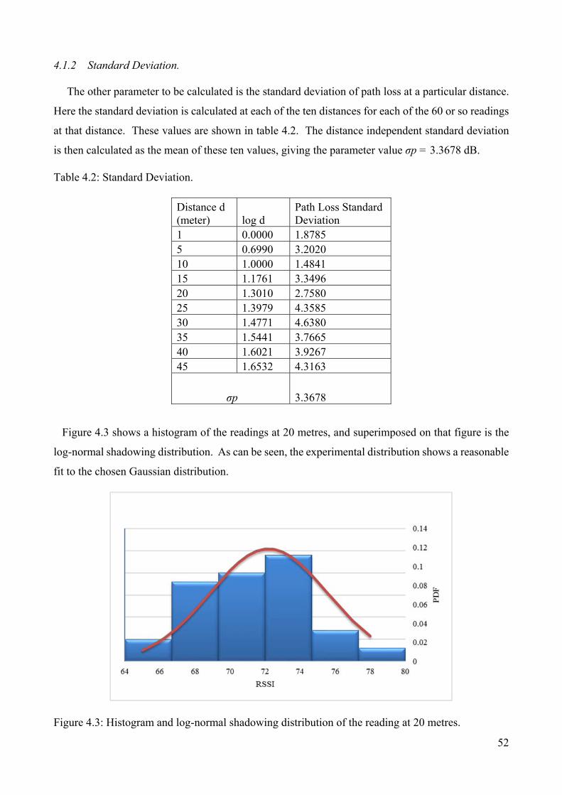
52
4.1.2 Standard Deviation.
The other parameter to be calculated is the standard deviation of path loss at a particular distance.
Here the standard deviation is calculated at each of the ten distances for each of the 60 or so readings
at that distance. These values are shown in table 4.2. The distance independent standard deviation
is then calculated as the mean of these ten values, giving the parameter value σp = 3.3678 dB.
Table 4.2: Standard Deviation.
Distance d (meter) log d
Path Loss Standard Deviation
1 0.0000 1.8785 5 0.6990 3.2020 10 1.0000 1.4841 15 1.1761 3.3496 20 1.3010 2.7580 25 1.3979 4.3585 30 1.4771 4.6380 35 1.5441 3.7665 40 1.6021 3.9267 45 1.6532 4.3163
σp 3.3678
Figure 4.3 shows a histogram of the readings at 20 metres, and superimposed on that figure is the
log-normal shadowing distribution. As can be seen, the experimental distribution shows a reasonable
fit to the chosen Gaussian distribution.
Figure 4.3: Histogram and log-normal shadowing distribution of the reading at 20 metres.

53
Table 4.3 shows the final log-normal shadowing parameters that are the best fit to the experimental
measurements. These parameters will be used in future simulation experiments. In some cases, the
experiments will investigate the impact of having a low, medium or high variability in the distance
estimation, using σp = 1dB, 3.3678 dB or 5dB respectively.
Table 4.3 Parameters for simulation.
Parameter Value
d0 (reference distance) 1m
(nominal path loss at 1 metre) 28.43dB
n (log normal shadowing power) 3.3647
(standard deviation of path loss) 3.3678dB
Overall, the probabilistic RSSI versus distance model as given by the parameters of the log
distance path loss model are subject to change in a new environment, such as changes in the radio
transceivers, changes in the mounting of the receivers and their antennas, and changes in the physical
environment. For this reason, these parameters should be estimated for each new configuration, using
a set of experiments similar to those in sub section 4.1. Ideally, such experiments would be conducted
using the same type of sensors and mobile sink to be deployed in the field.
Furthermore, the RF propagation patterns of these low power nodes, with low cost antennas, are
not ideal, and will most likely not produce a uniform 3D propagation pattern. This non-uniformity is
dealt with to some extent through the use of probabilistic propagation models. Antenna propagation
patterns and differences in the relative orientation of transmitter and receiver antennas are one of the
causes of the probabilistic ranges associated with RSSI values. These effects can also be reduced by
ensuring that the initial calibration experiments for the RSSI/range model parameters are conducted
with the same radios in approximately the same configurations as will be encountered in the actual
deployment.

54
CHAPTER 5
LOCALIZATION ACCURACY VERSUS THE NUMBER OF MOBILE ANCHOR
POSITIONS
The parameters obtained from the outdoor preliminary experiments as discussed in chapter 4 are
used to identify the range and position estimation based on the Log Normal Shadowing model. These
parameters consist of the nominal path loss, the log normal shadowing power and the standard
deviation of path loss. In this chapter, and in subsequent chapters, these values are used in
probabilistic simulations to investigate issues relevant to using an airborne mobile anchor for sensor
node localization.
This first research question involves detailed analysis on how the localization accuracy varies with
the number of mobile anchor node positions in a 3D localization scenario with an airborne mobile
anchor. Here, the commonly used Deterministic Multilateration (DML) algorithm will be used to
analyse whether the accuracy depends strongly on the positions of the mobile anchor node, how it
varies with the number of mobile anchor node positions, and how these dependencies are affected by
the level of variability of RSSI estimates of distance. The performance of the airborne mobile anchor
node is compared to fixed ground-based anchors, and to a combination of fixed and mobile anchor
nodes. These experiments will allow decisions to be made in subsequent experiments about how many
mobile anchor readings are needed for good localization.
As described in the literature review, DML uses a single best estimate of distance based on RSSI.
The use of RSSI was proposed in [40] and [99] as a source of ranging using only one mobile anchor
node. If the standard deviation of the log (distance) error is constant, then for lower RSSI, i.e. larger
distances, the absolute variability of distance error increases. With DML, all distance estimates have
equal weighting in the least-squares solution. So adding additional, inaccurate low-RSSI readings
may actually decrease the quality of the position estimates.
Therefore, this chapter first reviews the DML algorithm that is used in this research to localize
blind nodes in wireless sensor networks. Preliminary investigation was carried out to simulate typical
localization scenarios as mentioned in chapter 3. Simulation using Matlab is used with a statistical
model of RSSI versus distance for various scenarios, based on previously published work [100]. The
performance of localization accuracy that varies with the number of beacon positions and the RSSI
variability for various topologies will be analysed.

55
5.1 Deterministic Multilateration (DML).
This methodology section recaps the equations and notation that will be used to describe the DML
algorithm, described previously in Chapter 2. The range estimation in DML algorithm is based on the
Log Normal Shadowing model. By adapting equation (2.7) to find the path loss for a given distance,
the distance estimation dx between mobile anchor node and blind node can be calculated using
equation (2.8), repeated here for convenience.
dx = 10 * [((PL (dx) - PL (d0)) / (10.n)] (2.8)
Referring to figure 2.6 in chapter 2, multilateration solves the unknown position of node B, using
n beacons, numbered 1 to n, at positions [xi, yi, zi] and at estimated distance ri from node B. We can
define a matrix A with n-1 rows of the form;
[(xn – xi) (yn – yi) (zn – zi)] (5.1)
where xn, yn, and zn are the x,y and z position of the mobile anchor beacon position and xi, yi, and zi
are the position of the ith blind node position.
We also can define a column range vector, r, with each row of the form;
(1/2)((xn2 + yn
2 – rn2) - (xi
2 + yi2 – ri
2)) (5.2)
Then we solve for the blind node position;
x = [x y z]T (5.3)
By solving the matrix;
A x = r (5.4)
Giving x = A# r (5.5)
Where A# is the pseudo inverse, (AT .A)-1 . AT (5.6)
If there are more beacons than are required for a solution, the least-square error solution is provided
by this method.
5.2 Experimental setup.
The sensor nodes simulated in this experiment have a receiver sensitivity of -90.5dB, which is
equivalent to approximately 60 metres transmission range. Experiments are carried out in a simulated
space, which is 50m x 50m x 50m. This size of sensing region is suitable to localize a single blind

56
node. Based on the parameters from our real outdoor experiment as provided previously in table 4.3,
we used d0 = 1m, = 28.43dB, and n=3.3647 and a constant standard deviation (i.e., independent
of distance) for RSSI = 3.3678dB. Blind node localization is independent for each node, so these
experiments consider just one blind node placed on the ground at x=25m, y=25m, z=0m.
In the simulation, 15 mobile anchor beacon positions are used. The blind node makes distance
estimates to the 15 mobile anchor node positions based on RSSI from the mobile anchor node
beacons, drawn randomly from the Gaussian probability distributions. For these experiments, it is
assumed that the beacon positions are exact. To investigate the effect of different numbers of anchor
points on localization accuracy, the best “N” anchor points are chosen, with N varying from 4 (the
minimum needed for a solution) to 15 (total available beacons). For these experiments, “best’
corresponds to the N highest RSSI measurements, since smaller RSSI measurements typically give
higher range estimate errors. However, the geometric arrangement of the chosen “N” beacons are
not considered here, but this factor will be investigated further in chapter 7.
The experiments also investigate how the variability of RSSI impacts localization performance,
by varying the standard deviation of sampled RSSI values. For the medium variability case, a
constant standard deviation for RSSI = 3.3678dB is used, as obtained from field trials. Low
variability ( = 1dB) and high variability scenarios ( = 5dB) are also investigated through
simulation.
The following experiments are undertaken.
Experiment 1: 15 mobile anchor node points are chosen at random in the airspace above the blind
node.
Experiment 2: 15 mobile anchor node points are chosen along a pre-determined flight path, which
is between 1 and 10 metres above the ground. (Note that any planar flight path, such as constant
height, leads to flip ambiguity in localization, thus the height is varied). Figure 5.1 shows the anchor
points, and one example of the actual and estimated blind node position.
Experiment 3: 4 fixed anchors are placed on the ground at the corners of the area, at positions
(0,0,0), (0,50,0), (50,0,0), (50,50,0) and these are used to localize the node at (25,25,0).
Experiment 4: The 4 fixed anchors plus the 15 mobile anchor nodes are all used to localize the blind
node. The best N distance estimates out of the total 19 estimates are used. Only the best 15 positions
will be shown in the graph.

57
Experiment 5: This repeats experiment 4, but with the blind node in a poor geometrical position.
The node is placed outside the 50m x 50m x50m space at position (-10, -10, 0).
Figure 5.1: The actual and estimated blind node’s location on the ground with designated position of
anchor node.
For each individual experiment, a large number of trials are conducted and the average localization
error calculated. For experiment 1, each trial chooses different random anchor positions. For the
other experiments, the anchor positions are fixed across all trials – the only variability between trials
is the RSSI-based distance estimates. It was found that 100 trials were sufficient to get a stable average
error.
5.3 Results.
5.3.1 Localization of the blind node using random mobile anchor node positions.
Figure 5.2 and table 5.1 show the results for experiment 1. For high RSSI variability, 15 beacon
readings could not be achieved, hence the missing values listed for 12 beacons or greater. Anchor
positions are chosen randomly in the 50m x 50m x50m space, resulting in many long distances and
large RSSI errors. There is no clear pattern to the results.
Note that all of average localization error are in metre (m).

58
Figure 5.2: Localization error versus number of mobile anchor node with random positions for blind
node deployed on the ground.
Table 5.1 : Average localization error in metres for 15 mobile anchors with random positions for
different RSSI variability.
5.3.2 Localization of the blind node using designated flight path.
Figure 5.3 and table 5.2 show the results when a fixed set of 15 anchors below 10 metres in height
are chosen. The pattern here is clearer, and is similar for each level of variability. The error is
reasonably high for the best 4 anchors, decreases as more anchors are used up until about 13 anchors
for RSSI variability of 5dB. As the number of anchor increases, then, as additional “poorer” anchors
are used, the error increases again. This clearly shows that “more anchors are not always better”. A
preferred number of anchors can be identified that gives lowest error for a given variability and
standard deviation: 9 anchors for low variability, 11 anchors for medium variability, and 13 anchors
for high variability.
4 5 6 7 8 9 10 11 12 13 14 151 26.11 3.22 4.26 4.14 3.65 2.58 3.06 2.98 3.22 2.76 3.00 3.62
3.367 39.97 11.67 11.85 11.68 8.54 10.09 10.04 10.45 10.13 11.98 11.13 NA5 49.97 28.60 19.35 13.59 13.45 15.10 14.39 13.65 NA NA NA NA
Standard deviation
Number of anchor positions

59
Figure 5.3: Average localization error in metres for 15 mobile anchors with designated flightpath
positions for different RSSI variability.
Table 5.2: Localization error for 15 designated mobile anchor node at different RSSI variability.
5.3.3 Localization of the blind node using fixed static anchors.
Figure 5.4 and 5.5 show the results of experiment 3 with 4 fixed anchors at the ground-level corners
of the area at different location (25, 25, 0 and 40, 25, 0). Results with 4 fixed anchors are better than
the best 4 mobile anchors in figure 5.3, in term of localization error for different RSSI variability.
Figure 5.3 shows the localization error of 10 and 38 metre for 1dB and 3.367dB respectively, while
the localization error in Figure 5.4 is reduced to 3 and 9 metre respectively. This is because the four
fixed anchors are better positioned for localizing the blind node, which is located in the centre of
region (25, 25, 0). In this simulation, only nodes at low and medium variability can be localized.
Using high RSSI variability in localization will results to unlocalized node due to limitation of the
receiver sensitivity. However, the localization error may increase or may not be localized for other
layouts, for example when the blind node is located at 40, 25, 0 as shown in figure 5.5. Based on the
result, using four fixed anchor shows an improvement of localization error for certain layout.
Therefore, another extension of combination of these fixed anchors with the strongest mobile anchors
node will be analysed in the following section.
4 5 6 7 8 9 10 11 12 13 14 151 9.91 6.15 4.74 4.26 3.21 3.13 3.25 3.78 3.78 3.49 3.90 4.11
3.367 37.76 24.82 19.88 17.08 16.12 15.39 13.92 11.98 12.01 12.65 13.24 15.465 56.12 31.73 28.62 25.06 22.48 22.25 19.60 16.41 16.74 16.49 21.37 NA
Standard deviation
Number of anchor positions
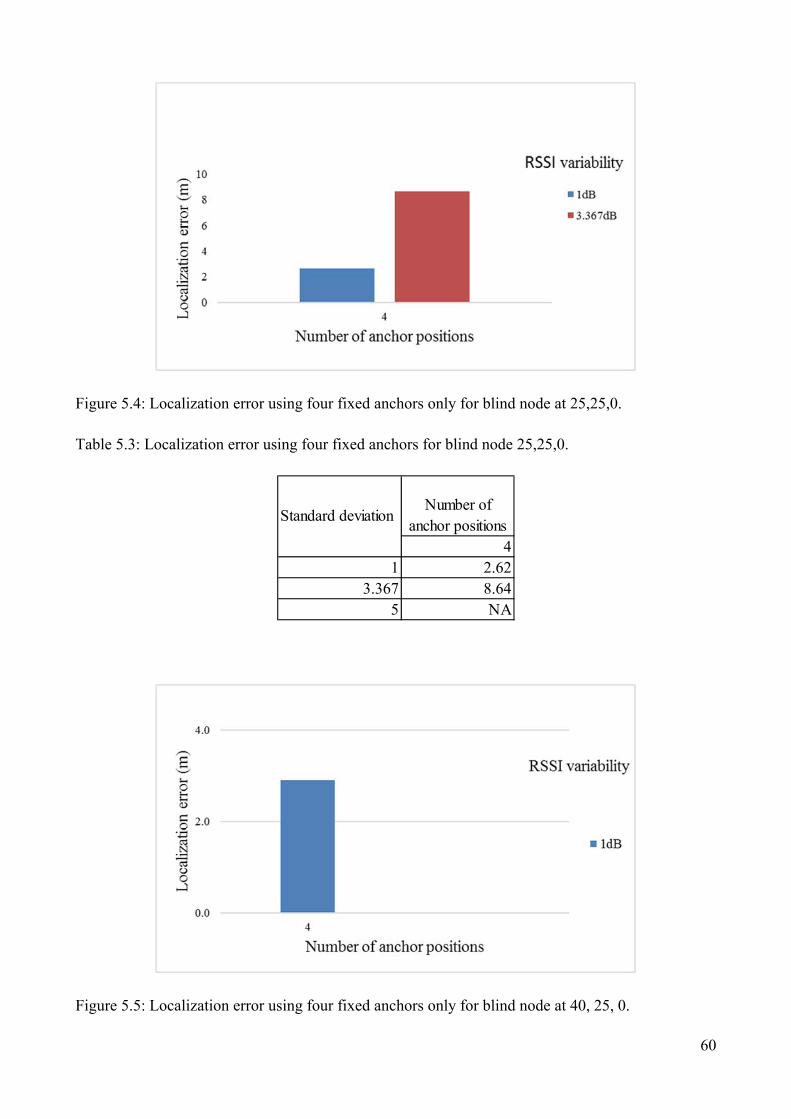
60
Figure 5.4: Localization error using four fixed anchors only for blind node at 25,25,0.
Table 5.3: Localization error using four fixed anchors for blind node 25,25,0.
Figure 5.5: Localization error using four fixed anchors only for blind node at 40, 25, 0.
41 2.62
3.367 8.645 NA
Standard deviationNumber of
anchor positions
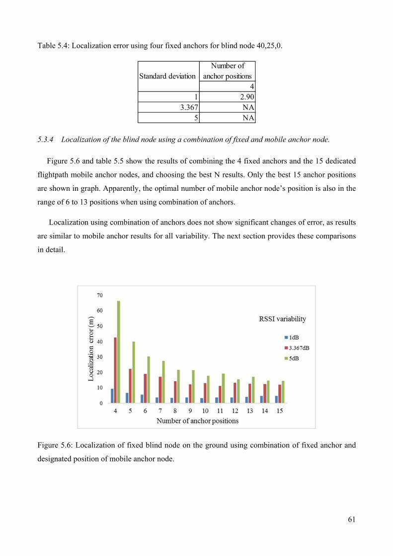
61
Table 5.4: Localization error using four fixed anchors for blind node 40,25,0.
5.3.4 Localization of the blind node using a combination of fixed and mobile anchor node.
Figure 5.6 and table 5.5 show the results of combining the 4 fixed anchors and the 15 dedicated
flightpath mobile anchor nodes, and choosing the best N results. Only the best 15 anchor positions
are shown in graph. Apparently, the optimal number of mobile anchor node’s position is also in the
range of 6 to 13 positions when using combination of anchors.
Localization using combination of anchors does not show significant changes of error, as results
are similar to mobile anchor results for all variability. The next section provides these comparisons
in detail.
Figure 5.6: Localization of fixed blind node on the ground using combination of fixed anchor and
designated position of mobile anchor node.
41 2.90
3.367 NA5 NA
Standard deviationNumber of
anchor positions

62
Table 5.5: Localization error for 15 anchors at different RSSI variability.
Additionally, combining four fixed anchors with the strongest mobile anchors might not always
be the best. Most of the fixed anchors for instance 0, 50, 0 has longer distance at 48 metres compared
to mobile anchor as shown in the following table.
Table 5.6: New position of anchor nodes (fixed and mobile anchor) based on the shortest estimated
distance in metre.
Estimated distance (m)
Anchor position X Y Z
3.82 25 25 6 6.60 30 30 5 11.40 20 30 5 18.41 40 25 7 19.72 15 35 6 19.72 30 10 10 19.72 40 15 10 22.61 10 40 7 25.92 50 20 9 27.76 15 45 9 29.72 10 0 10 29.72 20 0 10 29.72 25 40 10 34.08 50 0 0 39.08 50 50 0 44.81 0 0 0 47.99 0 0 10 47.99 0 50 0 55.03 5 50 8
5.3.4.1 Comparison of RSSI variabilities for fixed, mobile and combination anchor.
Figure 5.7 and table 5.7 compare the results of fixed (4 positions only), mobile (best 4 to 15) and
fixed and mobile (best 4 to 15). Figure 5.7 shows low variability, figure 5.8 shows medium variability,
while figure 5.9 shows high variability results. The error from the combination of anchors is equal to
or worse than the case of mobile anchor nodes only, again reflecting that “more anchors is not always
better”.
4 5 6 7 8 9 10 11 12 13 14 151 9.16 6.47 5.43 3.73 3.52 3.66 3.34 3.65 3.67 4.12 4.72 4.64
3.367 42.51 22.10 18.90 17.15 14.22 12.08 12.85 11.13 13.21 12.47 12.31 11.915 66.19 39.93 30.12 27.33 21.61 21.46 17.66 19.04 15.42 16.98 14.59 14.34
Standard deviation
Number of anchor positions
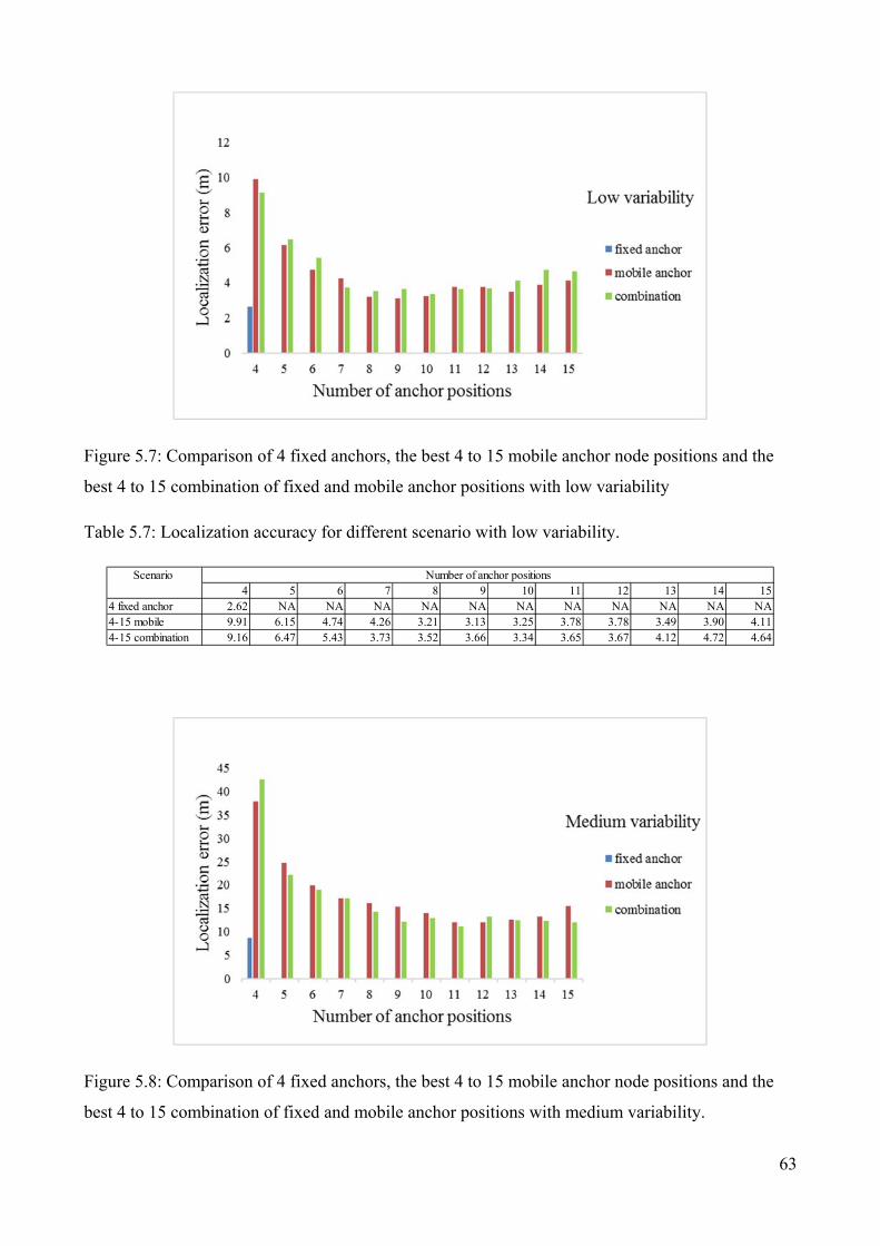
63
Figure 5.7: Comparison of 4 fixed anchors, the best 4 to 15 mobile anchor node positions and the
best 4 to 15 combination of fixed and mobile anchor positions with low variability
Table 5.7: Localization accuracy for different scenario with low variability.
Figure 5.8: Comparison of 4 fixed anchors, the best 4 to 15 mobile anchor node positions and the
best 4 to 15 combination of fixed and mobile anchor positions with medium variability.
4 5 6 7 8 9 10 11 12 13 14 154 fixed anchor 2.62 NA NA NA NA NA NA NA NA NA NA NA4-15 mobile 9.91 6.15 4.74 4.26 3.21 3.13 3.25 3.78 3.78 3.49 3.90 4.114-15 combination 9.16 6.47 5.43 3.73 3.52 3.66 3.34 3.65 3.67 4.12 4.72 4.64
Number of anchor positionsScenario

64
Table 5.8: Localization accuracy for different scenario with medium variability.
Figure 5.9: Comparison of 4 fixed anchors, the best 4 to 15 mobile anchor node positions and the best
4 to 15 combination of fixed and mobile anchor positions with high variability.
Table 5.9: Localization accuracy for different scenario with high variability.
5.3.5 Localization of the blind node at poor geometrical position.
Figure 5.10 and table 5.10 show the results when the node is away from the expected sensor space.
Due to poor geometric arrangement and being only able to reliably see 11 anchor points, error is very
high at around 99 metres at high variability for the best four anchor position.
4 5 6 7 8 9 10 11 12 13 14 154 fixed anchor 8.64 NA NA NA NA NA NA NA NA NA NA NA4-15 mobile 37.76 24.82 19.88 17.08 16.12 15.39 13.92 11.98 12.01 12.65 13.24 15.464-15 combination 42.51 22.10 18.90 17.15 14.22 12.08 12.85 11.13 13.21 12.47 12.31 11.91
Scenario Number of anchor positions
4 5 6 7 8 9 10 11 12 13 14 154 fixed anchor NA NA NA NA NA NA NA NA NA NA NA NA4-15 mobile 56.12 31.73 28.62 25.06 22.48 22.25 19.60 16.41 16.74 16.49 21.37 NA4-15 combination 66.19 39.93 30.12 27.33 21.61 21.46 17.66 19.04 15.42 16.98 14.59 14.34
Scenario Number of anchor positions
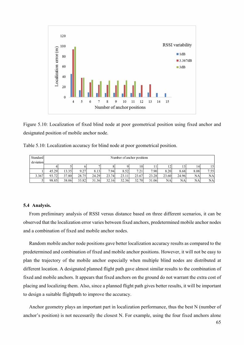
65
Figure 5.10: Localization of fixed blind node at poor geometrical position using fixed anchor and
designated position of mobile anchor node.
Table 5.10: Localization accuracy for blind node at poor geometrical position.
5.4 Analysis.
From preliminary analysis of RSSI versus distance based on three different scenarios, it can be
observed that the localization error varies between fixed anchors, predetermined mobile anchor nodes
and a combination of fixed and mobile anchor nodes.
Random mobile anchor node positions gave better localization accuracy results as compared to the
predetermined and combination of fixed and mobile anchor positions. However, it will not be easy to
plan the trajectory of the mobile anchor especially when multiple blind nodes are distributed at
different location. A designated planned flight path gave almost similar results to the combination of
fixed and mobile anchors. It appears that fixed anchors on the ground do not warrant the extra cost of
placing and localizing them. Also, since a planned flight path gives better results, it will be important
to design a suitable flightpath to improve the accuracy.
Anchor geometry plays an important part in localization performance, thus the best N (number of
anchor’s position) is not necessarily the closest N. For example, using the four fixed anchors alone
4 5 6 7 8 9 10 11 12 13 14 151 45.29 13.35 9.27 8.13 7.94 8.52 7.21 7.90 8.20 8.68 8.08 7.55
3.367 93.72 37.80 28.75 24.29 23.74 23.11 23.67 23.28 23.60 24.96 NA NA5 98.85 38.06 33.82 31.36 32.16 32.36 32.70 31.06 NA NA NA NA
Standard deviation
Number of anchor positions

66
gives better accuracy than using the “best” four from fixed and mobile anchor nodes. Therefore,
choosing anchors based on geometry needs to be considered, and this issue will be revisited later in
the thesis.
Less variability in RSSI readings obviously gave better results. For the best results, the average
localization error was about 3m for 1dB variability in RSSI, about 12m for 3.367dB variability and
about 14m for 5dB variability. Thus, it shows that the variability of RSSI will affect the localization
accuracy.
The fixed anchor scenario gave better results than the mobile anchor nodes for low variability,
most likely because of significantly better geometry, however localization with only fixed anchors
was not possible at high RSSI variability. Here, fixed anchors in ideal locations improve performance,
but this is not likely in a real scenario where there is no control over the node locations. Somewhat
surprisingly, the combined setup of fixed and mobile anchor nodes did not provide any significant
improvement in accuracy, due to the combination of poor anchor geometry, suggesting that the
mobile anchor node beacons are sufficient.
Also somewhat surprisingly, more anchor readings are not necessarily always better. The results
showed that approximately 6 to 13 anchor readings give the best compromise between the reduction
of errors from more readings and the increase in solution error by including low RSSI values. This
suggests more work is needed on how best to combine multiple RSSI readings. Alternatives include
the current “best N”, perhaps using all readings above a threshold, perhaps using probabilistic
methods to weight readings differently. A new algorithm based on probabilistic techniques will be
discussed further in the next chapter.
The DML algorithm examined here has poor performance in terms of location error. Within a
sensing area of 50x50m, localization errors are often above 20m. So rather than continuing
experiments based just on this traditional technique, other techniques should be explored.
Therefore, in the next chapter, a comparison of DML and our new approach called Volume
Probabilistic Multilateration (VPML) will be undertaken. The localization performance between
these two algorithms will be analysed based on the number of beacon packets. Furthermore, the
comparison in Chapter 6 will determine how to choose the best anchors from a larger set of possible
anchors.

67
CHAPTER 6
PROBABILISTIC MULTILATERATION
The previous chapter discussed how the localization performance of a mobile anchor varies with
different numbers of beacon packets using the DML algorithm. The performance has been compared
with fixed anchors and combinations of fixed and mobile anchors. The results also suggested that
more anchor readings are not necessarily always better. Furthermore, a significant issue with DML
is choosing the number of anchor readings that can give the best compromise between the reduction
of errors from more readings and the increase in solution error by including inaccurate RSSI distance
estimates. Therefore, probabilistic multilateration is investigated in this chapter, which seeks to use
information about the whole probability distribution of each RSSI-based distance estimate to choose
the blind node location with the highest likelihood.
In this chapter, an existing probabilistic technique, which I call Linear Probabilistic
Multilateration (LPML) is investigated. I then present an improved technique based on a new
formulation called Volume Probabilistic Multilateration algorithm (VPML) [101]. Additionally, the
performance of these two algorithms will be compared to the Deterministic Multilateration (DML)
as the RSSI variability changes. The results will allow choice of the best number of beacon positions
as well as the best localization algorithm in each context.
6.1 Probabilistic localization algorithms.
A single mobile anchor node will transmit anchor packets from multiple positions rather than use
RSSI distance estimates from static “anchor” nodes with known position as described in the work in
[40] and [99].
The work in [40] also determined the position of blind nodes with inaccurate range using multiple
and sparsely located mobile nodes. Location refinement is based on iterative and collaborative efforts.
The authors concluded that the probabilistic model is suitable for the outdoor environment and it
performed well compared to the proximity (range-free) measurement.
However, based on the existing research and the comparisons between probabilistic and
deterministic approaches in both works, limited work examines how many RSSI measurements are
needed for accurate localization, especially with a probabilistic method used for outdoor applications.

68
In this research, two probabilistic algorithms called Linear Probabilistic Multilateration (LPML)
and Volume Probabilistic Multilateration (VPML) algorithms will be used to investigate their relative
accuracy.
6.1.1 Linear Probabilistic Multilateration (LPML).
Ramadurai and Sichitiu [41] explain this LPML algorithm and this section describes their analysis.
In LPML, the distance between anchor node i (at position , and ) and blind node b (at
position , and ) can be calculated using the following equation:
(6.1)
Thus, the path loss can be defined as,
10 log (6.2)
where is the reference distance used for the experimental measurement which in this case is 1
metre, is the path loss at do, which for our experiments is 28.43dB, is the log normal shadowing
power, which for our experiments is 3.3647, and is the zero mean Gaussian random variable with
standard deviation of path loss , which is independent of distance. In our experiments, we use a
constant standard deviation for RSSI, which is 3.3678dB. In some cases, this will be varied to
understand the impact of RSSI variability.
In this probabilistic methodology, rather than only using a single estimate of position based on
RSSI, probabilistic localization uses the whole PDF of the RSSI versus distance distribution.
Therefore, given a , a PDF of possible distances from beacon i can be calculated as;
10 (6.3)
Equation (2.7) and (6.3) are the same, based on the Log Normal Shadowing model. Assuming
is 1 metre, then = 0
(6.4)
If is constant for all values of distance, d, then log can also be represented as a PDF of
RSSI:
(6.5)
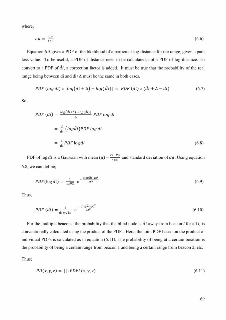
69
where,
(6.6)
Equation 6.5 gives a PDF of the likelihood of a particular log-distance for the range, given a path
loss value. To be useful, a PDF of distance need to be calculated, not a PDF of log distance. To
convert to a PDF of , a correction factor is added. It must be true that the probability of the real
range being between di and di+ must be the same in both cases.
∆ ∆ (6.7)
So;
∆
∆
log (6.8)
PDF of log is a Gaussian with mean ( = and standard deviation of . Using equation
6.8, we can define;
log √
(6.9)
Thus,
√
(6.10)
For the multiple beacons, the probability that the blind node is away from beacon i for all , is
conventionally calculated using the product of the PDFs. Here, the joint PDF based on the product of
individual PDFs is calculated as in equation (6.11). The probability of being at a certain position is
the probability of being a certain range from beacon 1 and being a certain range from beacon 2, etc.
Thus;
, , ∏ , , (6.11)

70
where is the PDF of being distance d from beacon i while is the un-normalized joint PDF
that the blind node is a certain distance from beacon 1 and a certain distance from beacon 2, until all
distances from each beacon i are estimated.
The actual PDF would require the PDF to be divided by the volume integral of the function above
to normalize the total likelihood of being anywhere in the volume to 1. However, the maximum value
of the joint PDF will only be considered here. The maximum of the un-normalized joint PDF will be
at the same location as a PDF normalized over the whole volume. An optimization approach, such
as gradient descent optimization, can then be used to find the point where PD(x,y,z) is a maximum,
and this is the estimated position. This is the conventional approach to probabilistic localization, as
described in [102].
6.1.2 Volume Probabilistic Multilateration (VPML).
A new Volume based PML formulation is devised, based on the Linear PML approach. The new
formulation of VPML is also described in our paper [101]. VPML shows superior results in
localization accuracy compared to Linear Probabilistic Multilateration (LPML) and Deterministic
Multilateration (DML) algorithm. Here, the performance of these three algorithms under different
RSSI variability conditions will be analysed to determine both the number of beacon positions that
minimises localization error and the best performing algorithm for each RSSI stability scenario.
LPML can be improved by a closer examination of how the individual PDFs are combined. In the
above formulation, each PDF is a function of a single variable, distance. Given that we are searching
for the best point in a 3-D space, it could also be argued that a PDF based on volume should be used,
not distance. Given a PDF(d) based on distance from a beacon, the PDF(x ,y, z) that the blind node
is at a particular point at that range can be calculated.
A point at a range of d in the one-dimensional PDF corresponds to the surface of a sphere, radius
d, centred at the beacon. The probability that the blind node is in an infinitesimal interval d+d in the
1-D PDF corresponds to the probability that the blind node is in a spherical shell, inner radius d, outer
radius d+d. The volume of the shell is surface area times thickness, 4πd2d. Since this shell volume
increases with d2, the volumetric PDF in 3-D will also scale with d2 compared to the linear PDF.
In particular, the volumetric PDF at a particular point on that sphere is
.
Again, ignoring constants (4π) and d, this gives a relative volumetric PDF for one beacon range
of:

71
(6.12)
Figure 6.1: 3 dimensional spatial PDF.
Then a new joint PDF for being at a certain point based on all the range estimates is:
, , ∏ , , (6.13)
In other words, we further scale each PDF by a factor of di2 before multiplying them together.
Next, we investigated which of , , and , , works best. In both cases a simple
gradient descent convex function optimization is used to find the maximum value of the joint PDF,
starting from the DML estimated position.
Gradient descent optimization is a mathematical search process which minimizes an objective
function by calculating the gradient of the function with respect to the inputs, and then taking a small
step in the direction of maximum negative gradient. The process is continued until the (local)
minimum is found. There are many different methods that can be used to select the appropriate
direction in which to move, and the size of the step in that direction. To take advantage of the state-
of-the-art optimization techniques, an existing gradient descent solver is used directly. For our
experiments, the MATLAB function fminunc is used for this optimization, and more details of the
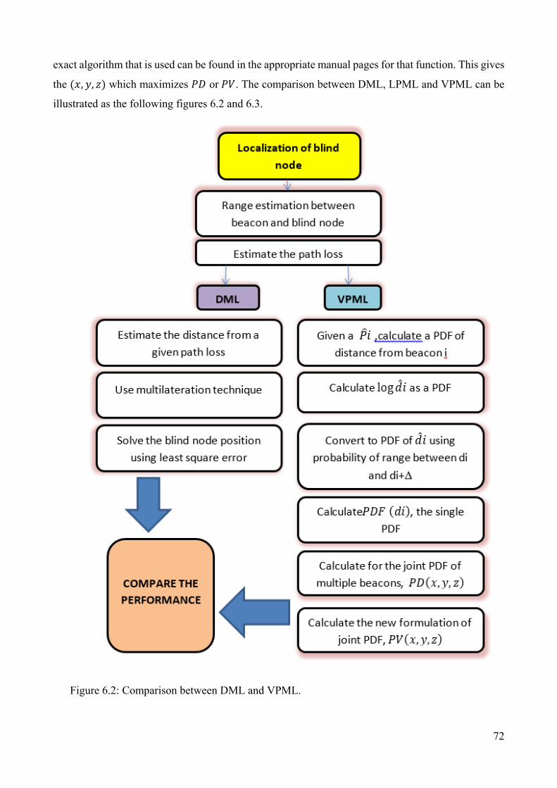
72
exact algorithm that is used can be found in the appropriate manual pages for that function. This gives
the , , which maximizes or . The comparison between DML, LPML and VPML can be
illustrated as the following figures 6.2 and 6.3.
Figure 6.2: Comparison between DML and VPML.

73
Figure 6.3: Comparison between LPML and VPML.
The key difference between LPML and VPML is the way in which the most likely candidate
position is calculated from the probabilities associated with a number of noisy range estimates. In

74
both cases, a joint probability function is calculated and a gradient descent search is performed to find
the point where the joint probability is maximised. For LPML, the joint probability distribution
function is simply the product of the individual linear PDFs of range estimates. However, as
explained earlier, a better joint PDF is one which estimates the probability of the point being in a
particular volume, and this requires scaling of the linear PDFs to be volume-based PDFs. This is the
extra step at the end of the right-hand flow in Figure 6.3. As will be shown by the experimental
results, this more theoretically correct method for combining the individual PDFs gives significantly
better position estimation results.
6.2 Experimental setup.
To compare the various algorithms MATLAB simulation of some typical scenarios will be used.
A simulated space, 50m x 50m x 50m, is used which is suitable to localize a single blind node. Blind
node localization is independent for each node, so these experiments consider there is just one blind
node placed on the ground. Random estimates of RSSI are generated based on the actual distances,
and the log-normal shadowing model which has been described in literature review section. We
conducted two experiments as follows.
Experiment 1: Experiment for single blind node localization at favourable and unfavourable
geometrical positions using DML and VPML.
The first experiment chooses 15 mobile anchor node points along a pre-determined flight path
which is between 1 and 11 metres above the ground with a blind node in a favourable location at
x=10m, y=10m, z=0m. Note that any planar flight path, such as constant height, leads to flip
ambiguity in localization, so it is important that the height of the aerial vehicle is varied. The
localization accuracy is then compared as different numbers of beacons are used for localization. The
number of beacons used is varied from N= 6 to 12. In every trial, the best N out of 15 are chosen,
where best means lowest path loss. The next experiment with the blind node in unfavourable
geometrical position is then repeated. The node is placed outside the 50m x 50m x50m space at
position (-10, -10, 0).
Experiment 2: Experiment for single blind node localization using DML, LPML and VPML
based on the RSSI variability.
These conducted experiments are similar to experiment 1, except that the standard deviation of
RSSI for a given distance is varied. Specifically, standard deviations of 1dB, 3.36 dB, and 5dB are
used for low, average, and high variability scenarios.
75
The localization accuracy of DML, LPML and VPML is then evaluated against the number of
beacons that are used for localization. The beacons are selected from the set of all available
measurements based on the lowest path loss. In each case, one set of stochastic RSSI readings are
calculated. These are used to find the best estimate of position, using each of the three techniques.
The simulation is repeated 100 times, and in each case, the positioning error is calculated.
Occasionally, the particular combination of geometry and probabilistic sampling of RSSI can lead
to a large error. If the mean value of location error across the 100 trials is used, these rare, large errors
can give significant perturbations in the mean value. Instead the median error from the 100 trials is
used, which gives more consistent results.
6.3 Results.
6.3.1 Localization single blind node localization at favourable and poor geometrical position using
DML and VPML.
Experiment 1 compares DML and VPML to investigate the usefulness of probabilistic techniques.
In experiment 2, LPML will also be included in the results.
Each experiment is repeated 100 times to avoid the effects of random variations in a single
experiment. Figure 6.4 and table 6.1 compare the median localization error of DML and VPML for
the first experiment. VPML clearly reduces the localization error as compared to DML by 57%-77%.
The localization error of VPML noticeably shrinks to 8 metres compared to DML with 35 metres as
the number of beacon positions increases and stabilizes for 10 to 12 positions. Thus, it shows that the
localization accuracy of VPML is better than DML. The performance of VPML is also varies with
the number of transmitted beacon positions. The results also indicate that 10 anchor readings with
VPML optimize the balance between the reduction of errors and the increase in solution error. The
figures show the median position error as well as the 10th/90th percentile values in the error bars that
is much lower with VPML than DML. Note that different positions of the blind node or mobile
anchors will produce different localization error results.

76
Figure 6.4 : Median localization error using N from 15 designated mobile anchor node positions with
DML and VPML for node in favourable position. 10/90 percentile ranges also shown.
Table 6.1: Localization median error (metres) and standard deviation (metres) for favourable blind
node position.
No of anchor positions 6 7 8 9 10 11 12DML 35.44 34.17 30.90 27.06 29.27 24.58 20.84VPML 8.03 7.91 8.57 7.92 8.93 8.93 9.36SD DML 28.54 25.85 22.30 24.56 25.97 21.13 21.01SD VPML 4.11 3.86 3.63 3.03 2.43 2.30 2.84

77
Figure 6.5: Median localization error using N from 15 designated mobile anchor node positions with
DML and VPML for node in unfavourable position. 10/90 percentile ranges shown.
Table 6.2: Localization median error (metres) and standard deviation (metres) for unfavourable
blind node position.
There is also a significant gap between error using DML and VPML in localizing the blind node
in a poor geometrical position as illustrated in Figure 6.5 and table 6.2. In fact, the error reduction of
VPML over DML for poor geometry is even larger than for the first experiment, confirming the
robustness of probabilistic localization.
The analysis shows that VPML performs better than DML and the localization error is reduced by
up to 80%. Approximately 6 to 12 RSSI readings are suggested for error reduction.
The new formulation of VPML works well since it reduces the influence of beacons that are far
from the blind node with more uncertain ranges.
No of anchor positions 6 7 8 9 10 11 12DML 95.00 108.26 81.31 86.79 114.84 94.95 99.81VPML 31.16 31.99 22.93 23.19 21.44 23.56 19.97SD DML 118.66 101.85 99.25 82.67 92.22 108.27 117.74SD VPML 17.30 15.06 15.90 12.93 10.88 12.23 11.07

78
6.3.2 Localization for single blind node localization using DML, LPML and VPML.
The median error as well as the range of the errors for three (3) RSSI standard deviation values
are calculated as shown in table 6.3 to 6.5. All distances are in metres.
6.3.2.1 DML versus LPML and VPML for low RSSI variability.
Figure 6.6 compares the localization error of DML, Linear PML and Volume based PML for a
typical arrangement of beacon positions and a blind node with standard deviation in the RSSI vs
distance PDF of 1dB. DML achieves its lowest localization error of 10 metre with 12 beacon
positions. However, its localization error is higher compared to the other two algorithms for the first
9 positions.
VPML clearly reduces the localization error as compared to DML by 35%-78% for 6 to 12
positions. Even though LPML shows improvement over DML from 6 to 9 beacon positions, its
localization error then gradually increases in contrast to DML and Volume based PML. VPML
outperforms LPML and its error decreases as more beacons are added. Thus it can be confirmed that
VPML performs better than LPML and can reduce the localization error to around 2 metre.
Both probabilistic approaches have noticeably lower variation in performance across the
simulation runs (as shown by the 10/90 percentile error bars) compared to DML. Table 6.3 also
shows the standard deviation of the location error across the 100 runs, which confirms this lower
variability.

79
Figure 6.6: DML versus LPML and VPML for standard deviation of 1dB.
Table 6.3: The median error and standard deviations (SD) of errors (in metres) for DML, LPML and VPML for standard deviation of 1 dB.
For DML, our previous experiments [100] have shown that using more than 12 beacons increases
error compared to using fewer lower path loss readings. All 15 nodes are used and it shows that the
simulation with very low RSSI have high inaccuracy. For instance, the median error of 12 positions
is 10 metre and it increased to more than 12 metre from 13 positions onward.
No of anchor positions 6 7 8 9 10 11 12DML 14.11 12.83 16.82 14.84 11.88 12.75 10.32LPML 7.55 6.25 10.51 12.75 13.22 14.96 16.24VPML 7.55 8.35 9.17 5.39 2.79 2.79 2.59SD DML 12.61 12.81 16.68 14.92 11.89 14.72 9.84SD LPML 0.94 1.82 1.70 1.25 0.66 1.23 0.78SD VPML 0.57 1.63 3.74 4.76 1.86 1.75 1.90

80
6.3.2.2 DML versus LPML and VPML for medium RSSI variability.
Experimental measurements of the RSSI standard deviation for the sensor nodes give a value of
3.36dB. Using this value in this simulation gives the results as in figure 6.7. The localization error
of VPML noticeably shrinks compared to DML from 40.9 metre to 7.7 metre and from 16.5 metre to
7.9 metre compared to Linear PML with 12 beacon positions. Thus, it is recommended to use between
6 to 12 beacon positions that give the lowest or near lowest localization error. Linear and Volume
based PML have superior performance to DML for any number of beacon positions with about 51%-
80% and 69%-78% respectively. The lowest median error achieved by Linear PML is 7.9 metres with
6 beacon positions, which is comparable to the results of Volume PML for 11 and 12 beacon
positions. The advantage of Volume based PML remains its stability and consistency of improving
the localization error over DML for both smaller RSSI variation (Figures 6.6) and moderate
variability (Figure 6.7).
Figure 6.7: DML versus LPML and VPML for standard deviation of 3.36dB

81
Table 6.4: The median error and standard deviations (SD) of errors (in metres) for DML, LPML and
VPML for standard deviation of 3.36dB.
6.3.2.3 DML versus LPML and VPML for high RSSI variability.
Figure 6.8 shows the results for an experiment with high RSSI variability. While LPML performs
better for lower number of beacon positions, VPML starts to improve the error over LPML from 9
beacon positions onward.
Additionally by comparing the three scenarios of differing variability, small standard deviation
(1dB) shows small improvement in error as the number of beacon positions increases. Scenarios with
standard deviation of 3.36dB and 5dB show more significant improvement over DML, even with
fewer beacon positions. VPML appears to have slightly higher variability in the results across
simulation runs compared to LPML with 9 to 12 beacon positions.
No of anchor positions 6 7 8 9 10 11 12DML 40.94 42.44 38.76 38.10 34.53 32.06 34.72LPML 7.92 9.62 11.36 12.98 14.37 15.56 16.54VPML 9.21 10.05 10.97 11.65 8.93 7.72 7.85SD DML 49.96 39.91 29.27 37.68 33.02 35.83 34.65SD LPML 6.03 2.71 1.84 1.89 1.20 1.50 1.86SD VPML 7.02 4.78 3.56 4.19 4.34 3.92 4.28

82
Figure 6.8: DML versus LPML and VPML for standard deviation of 5dB.
Table 6.5: The median error and standard deviations (SD) of errors (in metres) for DML, LPML and VPML for standard deviation of 5dB.
6.4 Analysis.
This experiments explored sensor node localization using the new formulation of Volume based
PML that gives significantly better error results for airborne beacon positions than the conventional
deterministic multilateration. The median error of VPML is reduced to around 3 metre and the
localization accuracy is improved by approximately 78%, at various RSSI variability values of 1dB,
3.36dB and 5dB. VPML’s error is considerably lower than DML and either lower than or comparable
to LPML, while delivering higher stability across different scenarios.
No of anchor positions 6 7 8 9 10 11 12DML 33.46 40.04 42.12 41.65 50.38 43.76 38.71LPML 6.57 8.62 10.26 11.64 12.82 13.65 14.79VPML 7.10 10.13 11.29 11.58 12.27 10.24 10.50SD DML 38.96 28.69 29.21 33.54 37.82 41.70 42.67SD LPML 3.31 3.09 3.25 2.38 3.62 2.25 2.24SD VPML 4.42 4.76 4.29 4.20 4.77 5.85 5.56

83
Currently, these experiments are done with fixed beacon positions. The “best” beacon positions
are selected based on signal strength. It is known that a good geometrical arrangement of beacons
can reduce localization error [67]. Therefore, the topic of the geometrical arrangement of beacons is
addressed in the next chapter. Experiments will be conducted to vary the height of beacons and the
distance or spacing between beacons and to investigate the effects on localization error using the
VPML algorithm.

84
CHAPTER 7
GEOMETRIC SENSITIVITY AND TRAJECTORY OF MOBILE ANCHOR NODE
7.1 Introduction.
A comparison of localization performance between probabilistic localization algorithms and the
deterministic algorithm has been discussed in previous chapter 5 and 6. Furthermore, a multilateration
algorithm and optimization of the number of anchors using DML and VPML algorithms also has
been analysed in [61]. However, there is limited analysis of geometric sensitivity of beacon positions
and mobile anchor trajectories. Thus, further research and experiments will be discussed in this
chapter.
In order to design the best flight path of the aircraft and to calculate the best beacon placement
along that flight path, this research aims to find good mobile anchor node positions for multiple blind
node localization on the ground. Good positioning involves tension between having high radio signal
strength, which gives lower ranging uncertainty and between having spaced out anchors. These
experiments also investigate how accuracy varies across the sensing region. Furthermore, the height
and the spacing between beacons and path length will be determined for the best compromise between
path length and accuracy.
This chapter investigates the number of simulation iterations that are needed to be give consistent
estimates of performance. Previously 100 iterations were used, but these experiments are more
complex (potentially thousands of beacons, tens of blind nodes), and so a smaller number of iterations
is helpful to reduce the experimental run time if it still gives consistent results.
The possible height of beacons and the spacing between beacons will be determined by
comparing different combinations of aircraft height and beacon spacing.
For a large number of beacons, the highest signal strength beacons may all be close together,
which is not a good geometry. The geometric arrangement of the beacons in terms of angles between
ranges to beacons will be examined.
A 1km x 1km sensing area is used to localize multiple blind nodes. There are 25 blind nodes
located near the centre, edges, corners and at other random positions on the ground within the sensing
region as in the following table.

85
Table 7.1: Position of 25 blind nodes (in metres).
As discussed in the literature review, various topologies of flights paths can be used – square grid,
circle, spiral, etc. Because the sensing area is square, a square grid is used consisting of rows of
beacons at one height then the next row at an alternate height to avoid flip ambiguity, as shown in
figure 7.3 and 7.4 later. The exact path between beacon positions may depend on aircraft dynamics,
but here the shortest path of straight lines between beacons is assumed here.
Five experiments will be conducted where the real distance is used with a random number
generator to give an estimated path loss between beacons and blind nodes. Any path loss that exceeds
the sensitivity of -90.5dB will be discarded. Then, a maximum of 20 of the strongest beacon packets
will be used to observe the relationship between number of anchor positions versus localization error.
Finally, the estimated position of the blind nodes using VPML will be determined. The parameters
used in this simulation are;
x y z1 50 750 02 158 823 03 250 1000 04 380 700 05 500 500 06 618 800 07 792 795 08 815 758 09 1000 1000 010 958 46 011 800 34 012 632 171 013 422 382 014 320 500 015 250 250 016 142 439 017 0 0 018 500 1000 019 700 200 020 906 743 021 127 192 022 913 655 023 98 706 024 278 32 025 850 300 0
Number Blind node positions
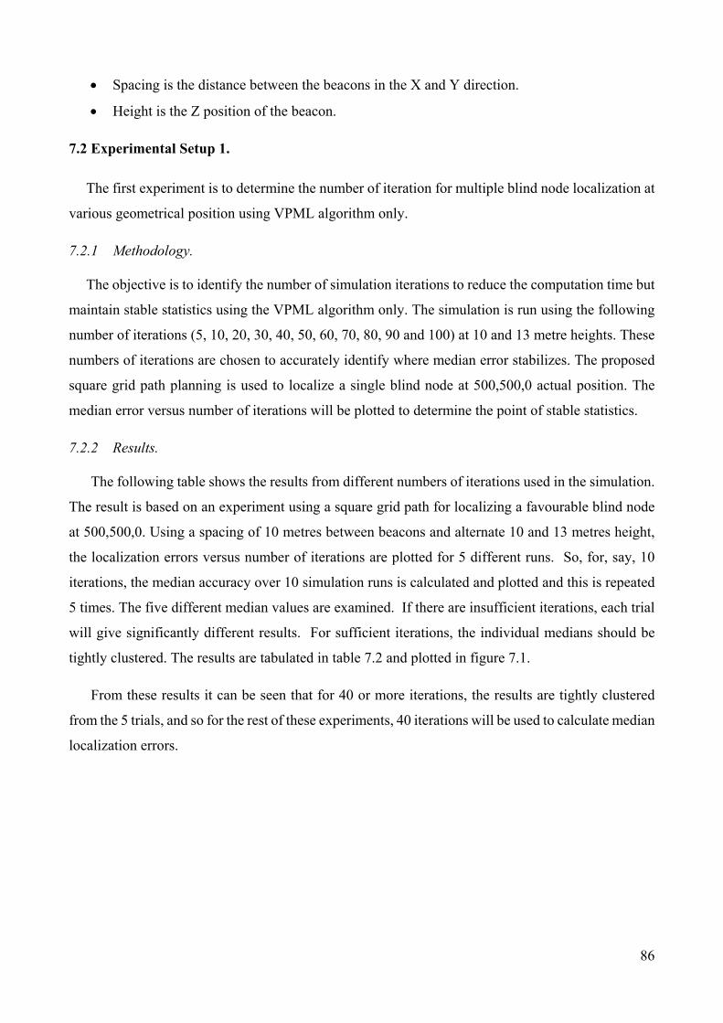
86
Spacing is the distance between the beacons in the X and Y direction.
Height is the Z position of the beacon.
7.2 Experimental Setup 1.
The first experiment is to determine the number of iteration for multiple blind node localization at
various geometrical position using VPML algorithm only.
7.2.1 Methodology.
The objective is to identify the number of simulation iterations to reduce the computation time but
maintain stable statistics using the VPML algorithm only. The simulation is run using the following
number of iterations (5, 10, 20, 30, 40, 50, 60, 70, 80, 90 and 100) at 10 and 13 metre heights. These
numbers of iterations are chosen to accurately identify where median error stabilizes. The proposed
square grid path planning is used to localize a single blind node at 500,500,0 actual position. The
median error versus number of iterations will be plotted to determine the point of stable statistics.
7.2.2 Results.
The following table shows the results from different numbers of iterations used in the simulation.
The result is based on an experiment using a square grid path for localizing a favourable blind node
at 500,500,0. Using a spacing of 10 metres between beacons and alternate 10 and 13 metres height,
the localization errors versus number of iterations are plotted for 5 different runs. So, for, say, 10
iterations, the median accuracy over 10 simulation runs is calculated and plotted and this is repeated
5 times. The five different median values are examined. If there are insufficient iterations, each trial
will give significantly different results. For sufficient iterations, the individual medians should be
tightly clustered. The results are tabulated in table 7.2 and plotted in figure 7.1.
From these results it can be seen that for 40 or more iterations, the results are tightly clustered
from the 5 trials, and so for the rest of these experiments, 40 iterations will be used to calculate median
localization errors.

87
Figure 7.1: Median error (m) versus number of iterations for 5 trials.
Table 7.2: Median errors (m) for each of 5 trials.
7.3 Experimental Setup 2.
The second experiment is to determine the possible height of beacons.
7.3.1 Methodology.
The square grid path is designed to send a beacon at every position with a particular X-Y spacing
and with alternate rows at different heights to localize a blind node. Two nodes at 500,500,0 (directly
under a beacon) and 127,192,0 (between beacons) are localized. The objective is to determine which
are the best heights for alternate rows of beacons in the square grid flightpath. Note that the heights
of the mobile anchor (consisting of alternate lower and upper paths) is initially tested using a range
of height combinations such as 10 and 13 metres, 10 and 15 metres, 20 and 23 metres and 20 and 25
metres. 10 metres is chosen as a minimum height to avoid obstacles such as trees.
Solutions will use the best N nodes, where N is varied from 4 to 20.
Trial5 10 20 30 40 50 60 70 80 90 100
1 2.81 6.97 7.07 7.50 6.92 6.74 7.11 7.10 6.94 7.06 7.072 4.62 6.68 6.49 6.05 7.08 6.90 7.08 7.22 6.61 6.99 7.183 6.45 6.68 6.22 6.06 7.16 6.79 6.99 7.19 6.94 7.02 7.044 7.74 7.05 6.73 7.36 7.10 7.13 7.15 7.17 7.09 6.90 6.985 7.57 6.40 6.88 6.74 6.87 6.90 7.24 7.14 6.96 6.99 7.20
Number of iteration

88
This experiment will also justify the combination of heights that will be used for future
simulations.
7.3.2 Results.
The results are shown in figure 7.2 and table 7.3 for the two nodes (out of 25 blind nodes). This
shows that the performance is significantly better for the 10/13m and 10/15m alternate heights for
both nodes. It also shows that error reduces as more beacons are used up to about 13 nodes, and does
not significantly improve beyond that. The next experiment will investigate the best heights using a
lower height of 10m and an upper height of 11-15m.
Figure 7.2: Comparison between height for blind node 127,192,0 and 500,500,0.

89
Table 7.3: Median localization error for blind node 127,192,0 and 500,500,0.
Table 7.3 shows the median localization error for blind node for different number of beacon
positions and when different height of beacon is applied. These numbers are chosen to fully explore
the range of possibilities.
7.4 Experimental Setup 3.
The third experiment is to determine the possible spacing between beacons.
7.4.1 Methodology.
This experiment is to compare the localization performance at different beacon spacing by using
square grid spacing of 5, 10, 20, 30, 40, 50 and 60 metres with alternate heights determined by the
results from the previous section. These values are chosen to span the range between very many
beacon packets at 5m spacing to very few packets at 60m. The maximum spacing of 60m is chosen
since this is approximately the maximum radio range for a receiver sensitivity of -90.5dB. In this
simulation, a square grid path with these different spacing and heights is used to localize one blind
node located centrally (500,500,0) within a 1km x 1km area using VPML with up to 20 beacon
packets. Examples of a square grid path with alternate heights and different beacon spacing are shown
in figures 7.3 and 7.4.
4 8.30 13.83 16.63 16.54 19.41 19.89 21.13 29.365 8.80 9.70 16.96 16.44 13.53 15.97 17.08 19.686 8.39 9.19 15.58 17.56 10.02 10.34 20.22 15.827 8.81 8.93 14.52 15.37 8.75 9.04 11.08 15.558 8.68 8.62 8.03 10.63 8.19 9.95 8.53 9.509 8.58 9.13 7.06 9.39 8.37 9.85 8.03 8.5910 7.52 9.64 6.14 7.54 7.83 8.06 7.28 7.8411 6.22 6.65 6.65 7.52 5.54 6.30 5.88 5.9112 5.24 5.31 5.51 7.23 3.62 4.68 5.80 7.0013 3.81 5.25 7.25 7.35 3.62 3.24 6.20 6.1014 4.15 4.11 6.45 5.88 4.19 4.08 5.12 6.0715 4.27 5.28 6.33 5.43 4.35 4.37 7.49 5.7016 4.40 4.07 6.14 6.74 4.56 4.19 5.30 5.9717 4.57 4.13 5.54 7.07 4.21 4.88 6.24 6.5518 4.00 3.71 5.98 5.31 3.93 4.74 7.01 6.2419 4.08 4.15 7.04 6.55 5.58 5.23 7.05 6.1220 4.63 5.12 5.96 6.32 4.81 4.94 5.78 5.57
Localization error (m)
Number of beacon positions
Size
10&13 10&15 20&23 20&25 10&13 10&15 20&23 20&25
127 192 0 500 500 0
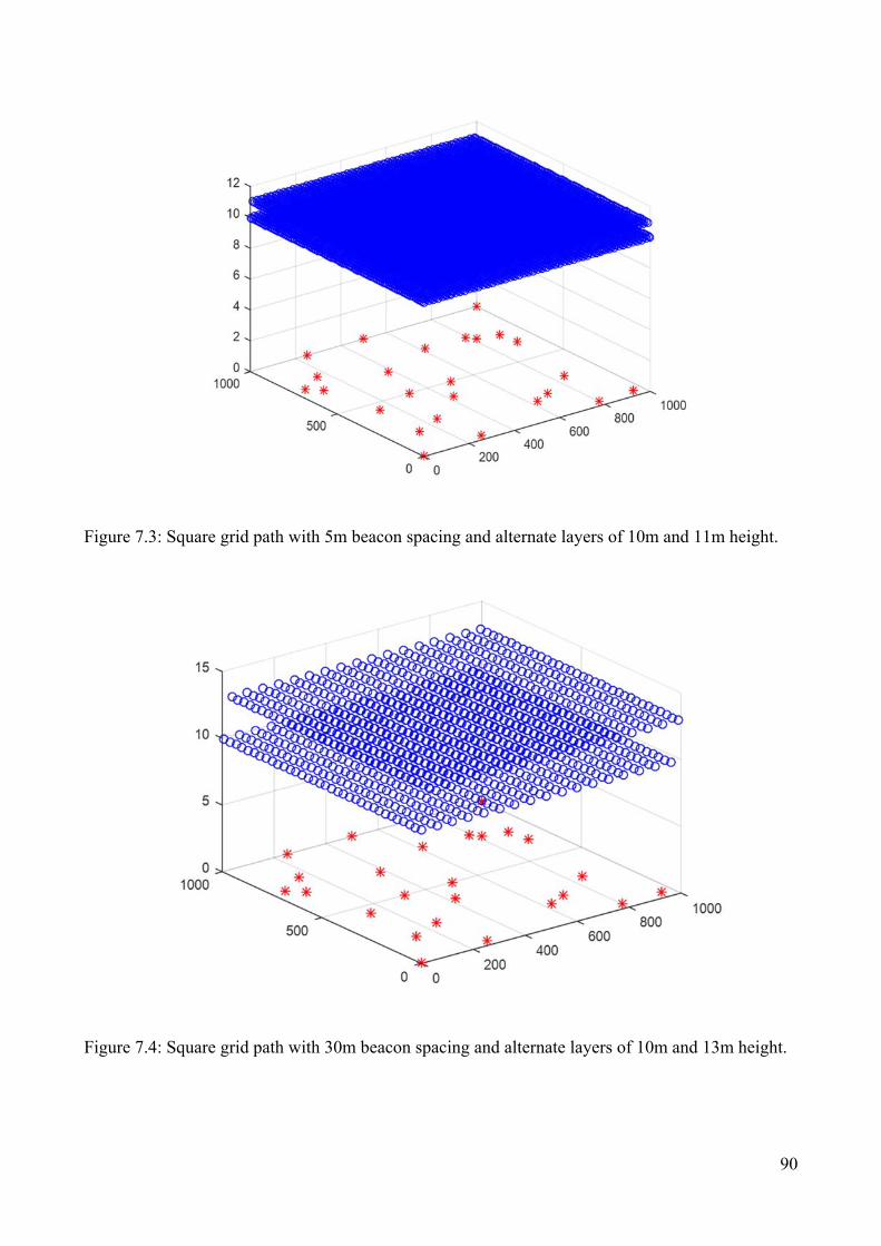
90
Figure 7.3: Square grid path with 5m beacon spacing and alternate layers of 10m and 11m height.
Figure 7.4: Square grid path with 30m beacon spacing and alternate layers of 10m and 13m height.
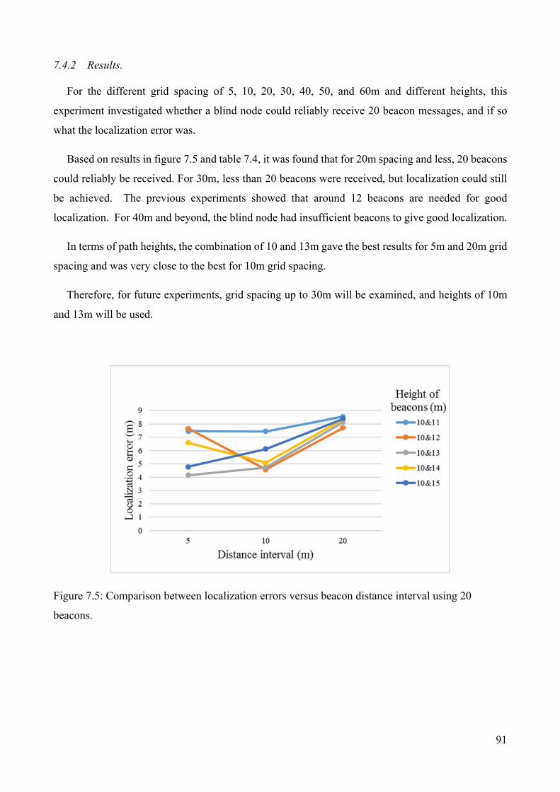
91
7.4.2 Results.
For the different grid spacing of 5, 10, 20, 30, 40, 50, and 60m and different heights, this
experiment investigated whether a blind node could reliably receive 20 beacon messages, and if so
what the localization error was.
Based on results in figure 7.5 and table 7.4, it was found that for 20m spacing and less, 20 beacons
could reliably be received. For 30m, less than 20 beacons were received, but localization could still
be achieved. The previous experiments showed that around 12 beacons are needed for good
localization. For 40m and beyond, the blind node had insufficient beacons to give good localization.
In terms of path heights, the combination of 10 and 13m gave the best results for 5m and 20m grid
spacing and was very close to the best for 10m grid spacing.
Therefore, for future experiments, grid spacing up to 30m will be examined, and heights of 10m
and 13m will be used.
Figure 7.5: Comparison between localization errors versus beacon distance interval using 20
beacons.

92
Table 7.4: Comparison of average localization error with 20 beacons based on beacon distance
interval (grid spacing) and height.
7.5 Experimental Setup 4.
The fourth experiment to determine the path length and number of beacons using the proposed
square grid path.
7.5.1 Methodology.
Using the square grid path planning with the best alternate heights from the previous experiment,
the various localization error for 25 blind nodes at various positions, as listed in Table 7.1, will be
identified. The number of transmitted beacons, minimum and maximum number of received beacons
and length of path can be retrieved. The maximum number of beacons is expected to vary depending
on the location of the blind node. The aim of this experiment is to compare the factors which
determine the time and energy needed by the mobile anchor to traverse the grid. These factors are
travel distance and number of transmitted beacons. Grid spacings of 5m, 10m, 20m and 30m are
used, with alternate heights of 10m & 13 m.
7.5.2 Results.
The following results (Figures 7.6, 7.7, 7.8 and tables 7.5, 7.6, 7.7) show the localization error for
3 blind nodes at different positions (the results for the other 22 blind nodes in Table 7.1 are shown in
Appendix B). The three nodes are located at favourable (500,500,0), unfavourable (0,0,0) and
between-beacon positions (142,439,0). The result is generated based on localization using a minimum
of 4 to a maximum of 20 anchor positions for square grid path planning using 40 simulation iterations
(the appropriate iterations based on the result from experiment 1). Table 7.8 shows the number of
beacons transmitted by the mobile anchor, the maximum and minimum number of received beacons
across the set of blind nodes and the length of each path.
5 10 20 30 40 50 6010 & 11 7.46 7.43 8.54 NA NA NA NA10 & 12 7.66 4.58 7.71 NA NA NA NA10 & 13 4.15 4.73 8.14 NA NA NA NA10 & 14 6.60 5.08 8.35 NA NA NA NA10 & 15 4.78 6.12 8.40 NA NA NA NA
Height of beacon (m)
Distance between beacon (m)

93
Figure 7.6: Comparison of average localization error between size for blind node 5 (500,500,0).
Table 7.5: Comparison of average localization error between size for blind node 5 (500,500,0).
5 10 20 30
4 8.22 8.23 7.54 7.615 8.85 8.18 7.47 8.986 8.74 8.99 6.42 9.927 8.41 8.43 6.06 7.458 8.47 9.79 6.11 8.889 11.84 8.63 7.75 9.74
10 8.34 8.02 7.45 8.8011 8.02 7.22 8.06 10.1712 7.64 4.86 6.74 10.0013 5.38 3.93 7.64 9.7414 3.81 3.57 5.61 8.6015 3.39 4.07 9.22 NA16 4.04 5.01 7.55 NA17 2.28 4.18 9.72 NA18 3.76 3.92 10.00 NA19 4.63 4.64 8.91 NA20 4.15 4.73 8.14 NA
Number of anchor positions
Spacing (m)

94
Figure 7.7: Comparison of average localization error between size for blind node (0,0,0).
Table 7.6: Comparison of average localization error between size for blind node (0,0,0).
5 10 20 304 8.26 10.39 15.70 21.335 9.26 11.45 16.97 18.736 11.17 12.89 21.36 NA7 9.86 13.54 22.36 NA8 10.60 14.69 12.17 NA9 11.45 15.67 17.07 NA
10 11.26 17.56 20.51 NA11 12.06 18.20 23.29 NA12 12.14 19.18 NA NA13 12.14 19.53 NA NA14 13.16 15.95 NA NA15 13.56 12.64 NA NA16 12.54 12.94 NA NA17 13.99 12.89 NA NA18 15.37 14.97 NA NA19 15.21 16.66 NA NA20 11.76 17.31 NA NA
Number of anchor positions
Spacing (m)

95
Figure 7.8: Comparison of average localization error between size for blind node (142,439,0).
Table 7.7: Comparison of average localization error between size for blind node (142,439,0).
Table 7.8 shows the minimum and maximum number of beacons available for use in localization
across the set of blind nodes. Note that a maximum of 20 nodes are used in the localization algorithm,
so even if more than 20 beacons are visible, only 20 are needed, and so the maximum is shown as 20.
5 10 20 304 14.39 8.63 7.32 8.225 8.03 8.48 7.54 11.276 8.20 8.37 6.75 9.147 8.72 8.55 6.06 9.678 13.96 8.52 6.88 6.719 8.34 8.57 7.91 10.9810 8.37 8.47 7.07 11.5611 10.16 8.08 7.14 9.4612 8.67 4.57 6.08 11.7013 5.54 6.09 7.41 10.1514 3.82 3.80 5.83 NA15 3.30 4.69 8.64 NA16 3.33 3.68 7.18 NA17 4.02 4.49 7.55 NA18 3.34 4.87 8.15 NA19 2.73 4.79 8.94 NA20 2.85 3.58 8.40 NA
Number of anchor positions
Spacing (m)

96
Table 7.8 Path characteristics for different grid spacing.
Characteristics Spacing
5m 10m 20m 30m
Maximum Beacons 20 20 20 14
Minimum Beacons 20 20 10 0
Transmitted Beacons 40200 10201 2601 1156
Length of Path 201km 102km 52km 35km
The result for blind node 500,500,0 in figure 7.6 above shows that with spacings of 5m and 10m,
the localization error reduces until about 14 beacons, and then it is relatively constant. However, the
errors for 20m spacing increase after 8 beacons and are relatively constant for 30m spacing up to the
maximum available beacons. Blind node 0,0,0 could only be localized using 5m and 10m spacing
with 20 beacon positions as shown in figure 7.7. For 20m and 30m spacing, error is large. The result
of blind node 142,439,0 as shown in figure 7.8 shows 20m spacing gives lowest error up to about 11
beacons, however the 20m error increases starting from 12 beacon positions. 5m and 10m spacing
continue to improve with more beacons.
Based on these results, 5m and 10m spacings give significantly better accuracy than 20m and 30m
spacings, provided that sufficient beacons (14 or more) are used. For most blind nodes, 20m spacing
still gives 20 available nodes, however for nodes near the edge this number falls significantly, and is
sometimes as low as 10, again suggesting 20m spacing is just at the edge of reliable localization, and
would only be recommended if the mobile anchor path length was a major factor.
However, there is not a clear advantage in using 5m spacing, and in some cases it gives poorer
results than 10m spacing. As can be seen from Table 7.8 above, it requires twice the travel distance
and 4 times as many radio transmissions, with negligible improvement in accuracy.
Therefore, for this particular scenario, a 10m spacing is the preferred option.
7.6 Experimental Setup 5.
The fifth experiment is to determine the geometric arrangement of the beacons.

97
7.6.1 Methodology.
The objective of this experiment is to look at the geometric arrangement of beacons for practical
grid spacings, to see if choosing the highest RSSI readings is always the best, and to also look to
explain some of the results from experiment 4 which show that in some cases, smaller grid spacing
gives worse results.
This experiment examines the relative angles between rays from the 20 closest beacons for 5, 10,
20 and 30m spacing only.
7.6.2 Results.
The results in the previous section show some initially counterintuitive results. Since a 5m spacing
grid already includes all of the x-y positions in a 10m grid, plus ones in between, it seems that it
should give better results.
However, the reason can be explained by looking at the geometric arrangement of the strongest
beacons, i.e. the closest beacons. Consider the 20 closest beacons around a blind node.
Figure 7.9 shows 5m spacing beacons around a blind node at position 500,500,0. A simulation is
run and the beacons are ordered in terms of strongest RSSI for that trial indicated by the number of 1
to 20 as shown in the figure. Notice that these are not necessarily the closest beacons because of
RSSI variability. The new arrangement of anchor positions after the simulation based on the strongest
RSSI is shown in table 7.9.
There are the similar results for a 10m spacing and 20m spacing in Figures 7.10 and 7.11 and Table
7.10 and 7.11. The figures and tables show the new arrangement of the anchor positions based on the
strongest RSSI after the simulation. For 20 metre spacing, only 18 beacons with strongest RSSI are
available for estimating the blind node position. The unavailability of the other two beacons is due to
its range exceeding the sensitivity.
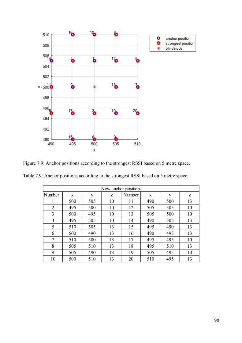
98
Figure 7.9: Anchor positions according to the strongest RSSI based on 5 metre space.
Table 7.9: Anchor positions according to the strongest RSSI based on 5 metre space.
Number x y z Number x y z1 500 505 10 11 490 500 132 495 500 10 12 505 505 103 500 495 10 13 505 500 104 495 505 10 14 490 505 135 510 505 13 15 495 490 136 500 490 13 16 490 495 137 510 500 13 17 495 495 108 505 510 13 18 495 510 139 505 490 13 19 505 495 10
10 500 510 13 20 510 495 13
New anchor positions
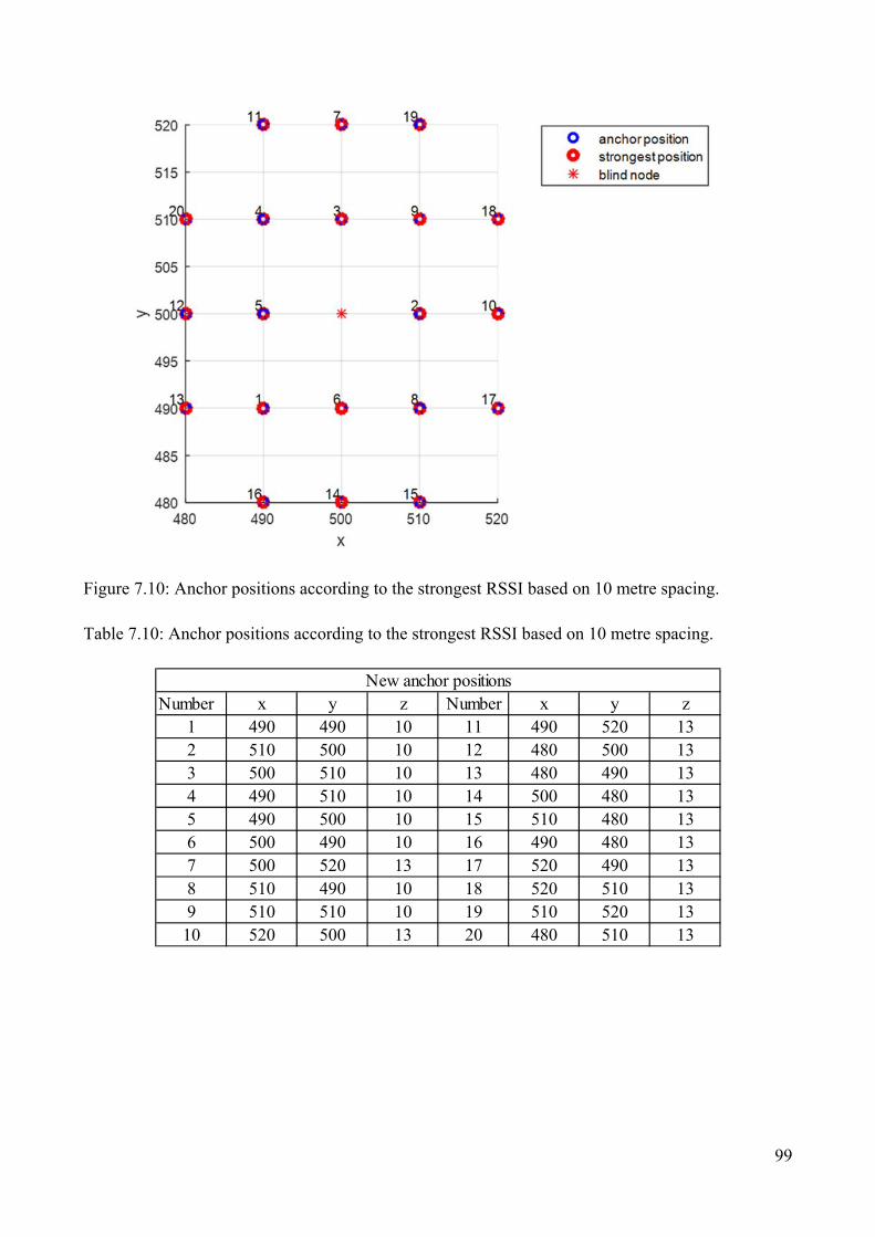
99
Figure 7.10: Anchor positions according to the strongest RSSI based on 10 metre spacing.
Table 7.10: Anchor positions according to the strongest RSSI based on 10 metre spacing.
Number x y z Number x y z1 490 490 10 11 490 520 132 510 500 10 12 480 500 133 500 510 10 13 480 490 134 490 510 10 14 500 480 135 490 500 10 15 510 480 136 500 490 10 16 490 480 137 500 520 13 17 520 490 138 510 490 10 18 520 510 139 510 510 10 19 510 520 13
10 520 500 13 20 480 510 13
New anchor positions

100
Figure 7.11: Anchor positions according to the strongest RSSI based on 20 metre spacing.
Table 7.11: Anchor positions according to the strongest RSSI based on 20 metre spacing.
Next, the angles between each pair of rays between beacons and blind node can be calculated.
These are shown in the tables 7.12-7.14 below. Note that the numbering of beacons is in terms of
decreasing RSSI. For example, in table 7.12, the angle between beacon 1 (B1) to the blind node and
beacon 2 (B2) to the blind node from figure 7.9 is 37 degrees, while the angle between B1 to the blind
node and B3 to the blind node is 53 degrees. Detail explanations regarding the significance of these
angles between each pair of rays is given later in this section.

101
Table 7.12: Angle between beacons for 5m spacing.
B1-B2 37 B3-B7 45 B5-B16 81 B8-B17 75 B12-B19 48B1-B3 53 B3-B8 65 B5-B17 75 B8-B18 34 B12-B20 42B1-B4 24 B3-B9 20 B5-B18 55 B8-B19 60 B13-B14 65B1-B5 36 B3-B10 64 B5-B19 42 B8-B20 55 B13-B15 57B1-B6 64 B3-B11 45 B5-B20 34 B9-B10 76 B13-B16 65B1-B7 45 B3-B12 57 B6-B7 51 B9-B11 65 B13-B17 57B1-B8 20 B3-B13 37 B6-B8 76 B9-B12 60 B13-B18 57B1-B9 65 B3-B14 57 B6-B9 17 B9-B13 36 B13-B19 24
B1-B10 11 B3-B15 20 B6-B10 75 B9-B14 76 B13-B20 20B1-B11 45 B3-B16 36 B6-B11 51 B9-B15 34 B14-B15 55B1-B12 24 B3-B17 24 B6-B12 67 B9-B16 55 B14-B16 34B1-B13 37 B3-B18 65 B6-B13 45 B9-B17 42 B14-B17 42B1-B14 36 B3-B19 24 B6-B14 65 B9-B18 81 B14-B18 24B1-B15 65 B3-B20 36 B6-B15 17 B9-B19 13 B14-B19 75B1-B16 57 B4-B5 60 B6-B16 39 B9-B20 24 B14-B20 81B1-B17 57 B4-B6 67 B6-B17 26 B10-B11 51 B15-B16 24B1-B18 20 B4-B7 67 B6-B18 76 B10-B12 26 B15-B17 13B1-B19 57 B4-B8 42 B6-B19 26 B10-B13 45 B15-B18 71B1-B20 57 B4-B9 75 B6-B20 39 B10-B14 39 B15-B19 42B2-B3 37 B4-B10 26 B7-B8 39 B10-B15 76 B15-B20 55B2-B4 24 B4-B11 26 B7-B9 39 B10-B16 65 B16-B17 13B2-B5 65 B4-B12 48 B7-B10 51 B10-B17 67 B16-B18 55B2-B6 45 B4-B13 57 B7-B11 75 B10-B18 17 B16-B19 60B2-B7 64 B4-B14 13 B7-B12 26 B10-B19 67 B16-B20 71B2-B8 57 B4-B15 60 B7-B13 11 B10-B20 65 B17-B18 60B2-B9 57 B4-B16 42 B7-B14 76 B11-B12 67 B17-B19 48
B2-B10 45 B4-B17 48 B7-B15 65 B11-B13 64 B17-B20 60B2-B11 11 B4-B18 13 B7-B16 76 B11-B14 17 B18-B19 75B2-B12 57 B4-B19 71 B7-B17 67 B11-B15 39 B18-B20 76B2-B13 53 B4-B20 75 B7-B18 65 B11-B16 17 B19-B20 13B2-B14 20 B5-B6 65 B7-B19 26 B11-B17 26B2-B15 36 B5-B7 17 B7-B20 17 B11-B18 39B2-B16 20 B5-B8 24 B8-B9 71 B11-B19 67B2-B17 24 B5-B9 55 B8-B10 17 B11-B20 76B2-B18 36 B5-B10 39 B8-B11 65 B12-B13 24B2-B19 57 B5-B11 76 B8-B12 13 B12-B14 60B2-B20 65 B5-B12 13 B8-B13 36 B12-B15 75B3-B4 57 B5-B13 20 B8-B14 55 B12-B16 75B3-B5 57 B5-B14 71 B8-B15 81 B12-B17 71B3-B6 11 B5-B15 76 B8-B16 76 B12-B18 42
Angle between each beacons:
5Size (m)8.55Localization error (m)
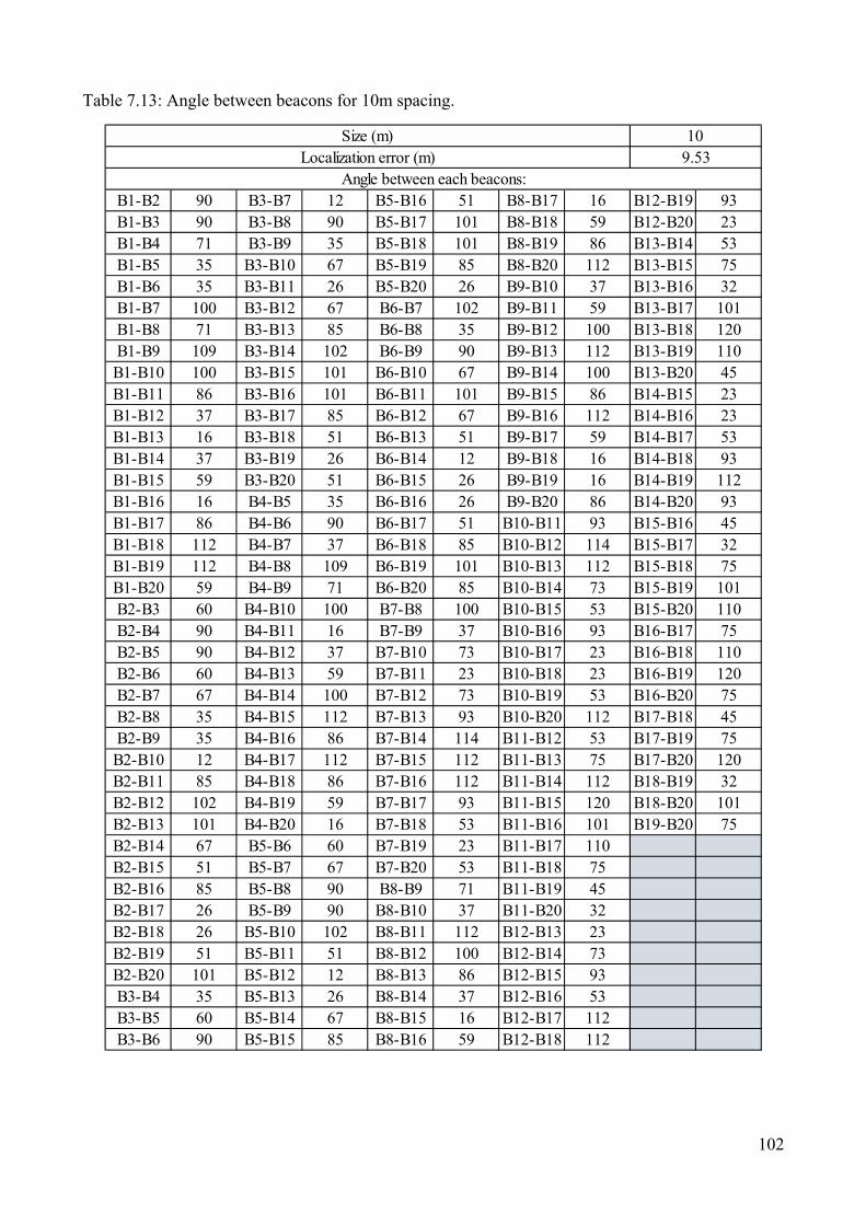
102
Table 7.13: Angle between beacons for 10m spacing.
B1-B2 90 B3-B7 12 B5-B16 51 B8-B17 16 B12-B19 93B1-B3 90 B3-B8 90 B5-B17 101 B8-B18 59 B12-B20 23B1-B4 71 B3-B9 35 B5-B18 101 B8-B19 86 B13-B14 53B1-B5 35 B3-B10 67 B5-B19 85 B8-B20 112 B13-B15 75B1-B6 35 B3-B11 26 B5-B20 26 B9-B10 37 B13-B16 32B1-B7 100 B3-B12 67 B6-B7 102 B9-B11 59 B13-B17 101B1-B8 71 B3-B13 85 B6-B8 35 B9-B12 100 B13-B18 120B1-B9 109 B3-B14 102 B6-B9 90 B9-B13 112 B13-B19 110
B1-B10 100 B3-B15 101 B6-B10 67 B9-B14 100 B13-B20 45B1-B11 86 B3-B16 101 B6-B11 101 B9-B15 86 B14-B15 23B1-B12 37 B3-B17 85 B6-B12 67 B9-B16 112 B14-B16 23B1-B13 16 B3-B18 51 B6-B13 51 B9-B17 59 B14-B17 53B1-B14 37 B3-B19 26 B6-B14 12 B9-B18 16 B14-B18 93B1-B15 59 B3-B20 51 B6-B15 26 B9-B19 16 B14-B19 112B1-B16 16 B4-B5 35 B6-B16 26 B9-B20 86 B14-B20 93B1-B17 86 B4-B6 90 B6-B17 51 B10-B11 93 B15-B16 45B1-B18 112 B4-B7 37 B6-B18 85 B10-B12 114 B15-B17 32B1-B19 112 B4-B8 109 B6-B19 101 B10-B13 112 B15-B18 75B1-B20 59 B4-B9 71 B6-B20 85 B10-B14 73 B15-B19 101B2-B3 60 B4-B10 100 B7-B8 100 B10-B15 53 B15-B20 110B2-B4 90 B4-B11 16 B7-B9 37 B10-B16 93 B16-B17 75B2-B5 90 B4-B12 37 B7-B10 73 B10-B17 23 B16-B18 110B2-B6 60 B4-B13 59 B7-B11 23 B10-B18 23 B16-B19 120B2-B7 67 B4-B14 100 B7-B12 73 B10-B19 53 B16-B20 75B2-B8 35 B4-B15 112 B7-B13 93 B10-B20 112 B17-B18 45B2-B9 35 B4-B16 86 B7-B14 114 B11-B12 53 B17-B19 75
B2-B10 12 B4-B17 112 B7-B15 112 B11-B13 75 B17-B20 120B2-B11 85 B4-B18 86 B7-B16 112 B11-B14 112 B18-B19 32B2-B12 102 B4-B19 59 B7-B17 93 B11-B15 120 B18-B20 101B2-B13 101 B4-B20 16 B7-B18 53 B11-B16 101 B19-B20 75B2-B14 67 B5-B6 60 B7-B19 23 B11-B17 110B2-B15 51 B5-B7 67 B7-B20 53 B11-B18 75B2-B16 85 B5-B8 90 B8-B9 71 B11-B19 45B2-B17 26 B5-B9 90 B8-B10 37 B11-B20 32B2-B18 26 B5-B10 102 B8-B11 112 B12-B13 23B2-B19 51 B5-B11 51 B8-B12 100 B12-B14 73B2-B20 101 B5-B12 12 B8-B13 86 B12-B15 93B3-B4 35 B5-B13 26 B8-B14 37 B12-B16 53B3-B5 60 B5-B14 67 B8-B15 16 B12-B17 112B3-B6 90 B5-B15 85 B8-B16 59 B12-B18 112
Size (m) 10Localization error (m) 9.53
Angle between each beacons:

103
Table 7.14: Angle between beacons for 20m spacing.
B1-B2 117 B3-B7 117 B5-B16 105 B8-B17 51 B12-B19B1-B3 117 B3-B8 130 B5-B17 27 B8-B18 131 B12-B20B1-B4 42 B3-B9 105 B5-B18 105 B8-B19 B13-B14 43B1-B5 42 B3-B10 135 B5-B19 B8-B20 B13-B15 85B1-B6 141 B3-B11 105 B5-B20 B9-B10 60 B13-B16 137B1-B7 84 B3-B12 27 B6-B7 84 B9-B11 118 B13-B17 60B1-B8 68 B3-B13 82 B6-B8 101 B9-B12 131 B13-B18 25B1-B9 101 B3-B14 42 B6-B9 68 B9-B13 137 B13-B19
B1-B10 43 B3-B15 9 B6-B10 122 B9-B14 140 B13-B20B1-B11 18 B3-B16 59 B6-B11 140 B9-B15 109 B14-B15 43B1-B12 101 B3-B17 130 B6-B12 68 B9-B16 51 B14-B16 101B1-B13 43 B3-B18 59 B6-B13 122 B9-B17 86 B14-B17 101B1-B14 84 B3-B19 B6-B14 84 B9-B18 148 B14-B18 18B1-B15 122 B3-B20 B6-B15 43 B9-B19 B14-B19B1-B16 140 B4-B5 78 B6-B16 18 B9-B20 B14-B20B1-B17 18 B4-B6 117 B6-B17 140 B10-B11 60 B15-B16 60B1-B18 68 B4-B7 117 B6-B18 101 B10-B12 137 B15-B17 137B1-B19 B4-B8 105 B6-B19 B10-B13 85 B15-B18 60B1-B20 B4-B9 130 B6-B20 B10-B14 122 B15-B19B2-B3 78 B4-B10 82 B7-B8 18 B10-B15 144 B15-B20B2-B4 127 B4-B11 27 B7-B9 18 B10-B16 109 B16-B17 131B2-B5 78 B4-B12 59 B7-B10 43 B10-B17 25 B16-B18 118B2-B6 42 B4-B13 9 B7-B11 101 B10-B18 109 B16-B19B2-B7 42 B4-B14 42 B7-B12 140 B10-B19 B16-B20B2-B8 59 B4-B15 82 B7-B13 122 B10-B20 B17-B18 86B2-B9 27 B4-B16 130 B7-B14 141 B11-B12 86 B17-B19
B2-B10 82 B4-B17 59 B7-B15 122 B11-B13 25 B17-B20B2-B11 130 B4-B18 27 B7-B16 68 B11-B14 68 B18-B19B2-B12 105 B4-B19 B7-B17 68 B11-B15 109 B18-B20B2-B13 135 B4-B20 B7-B18 140 B11-B16 148 B19-B20B2-B14 117 B5-B6 117 B7-B19 B11-B17 35B2-B15 82 B5-B7 42 B7-B20 B11-B18 51B2-B16 27 B5-B8 27 B8-B9 35 B11-B19B2-B17 105 B5-B9 59 B8-B10 25 B11-B20B2-B18 130 B5-B10 9 B8-B11 86 B12-B13 60B2-B19 B5-B11 59 B8-B12 148 B12-B14 18B2-B20 B5-B12 130 B8-B13 109 B12-B15 25B3-B4 78 B5-B13 82 B8-B14 140 B12-B16 86B3-B5 127 B5-B14 117 B8-B15 137 B12-B17 118B3-B6 42 B5-B15 135 B8-B16 86 B12-B18 35
Size (m) 20Localization error (m) 7.94
Angle between each beacons:

104
Now some of the anomalous examples in the previous section (in figure 7.6) can be examined in
a little more detail.
Consider first the example of using the strongest 7 beacons, where 20m spacing gave significantly
better accuracy than 5m spacing or 10m spacing. For 5m spacing, the tables show that the inter-ray
angles for the strongest 7 beacons vary from 17 to 67 degrees, so the angles are reasonably acute. For
10m spacing the range of angles is 12 to 102 degrees. For 20m spacing, the range is 42 to 141 degrees.
As was discussed in the literature review, angles around 90 degrees are thought to best for
localization, and this result supports that finding. Since the 20m spacing has a greater proportion of
such angles between the top 7 beacons, this results in better localization.
Next consider 12 beacons, where in figure 7.6, error for 10m spacing was considerably better than
5m spacing, and 20m spacing was about the same as 5m spacing. The ranges of angles for 5m beacons
in table 7.12 are 11 to 81 degrees, for 10m spacing in table 7.13 are 12 to 120 degrees, and for 20m
spacing in table 7.14 are 18 to 148 degrees. So here, the 10m spacing has a significant proportion of
its angles around 90 degrees, and so its better geometric arrangement gives better accuracy, even
though the individual range measurements are less accurate than for 5m spacing. However, its better
range estimation accuracy gives it better localization accuracy than 20m, which also has suitable
geometry.
For 20 beacons, 5m spacing still has the same range of angles, however the additional beacon
readings allow its accuracy to be significantly improved and are comparable to 10m spacing.
Overall, this short and limited investigation suggests that better geometric arrangement can
overcome poorer estimates of range. Furthermore, it suggests that if many beacons are available,
then the “best” beacons are not necessarily the strongest RSSI beacons. Instead, there will be a
compromise between selecting close beacons and geometrically well-located beacons. This could be
done in an iterative fashion – firstly doing a coarse quantisation, e.g. using the centroid of the beacon
XY positions and assuming zero height, then calculating the angles between various pairs of beacon
rays to the blind node, and then selecting nodes which gave a reasonable number of angles around 90
degrees.
A more detailed examination of the best way to select the geometrically best beacons is outside
the scope of this thesis, but would be an obvious next step for future work.

105
7.7 Conclusions.
These experiments aim to address the trade-off between the energy costs of travelling and
transmitting the beacons versus the accuracy of the localization, as well as choosing a good path
geometry. The results here are not universal results, and they do not give a flight path that is suitable
for all sensor deployments. What they do is describe a methodology by which such decisions can be
made through simulation of a specific scenario.
Firstly, a square grid with alternate height rows has been shown to give good localization which
avoids flip ambiguity. A square grid is suitable for a square search area compared to some of the
other possible paths described in section 2.10, such as circles or zig-zag paths, and it is the only
geometry considered in detail here. Different generic flightpaths could be more appropriate for
different shaped deployment areas.
Secondly, simulation of different alternate heights can be used to determine suitable heights which
minimize errors. In this case 10m and 13m were identified as best.
Thirdly, an initial investigation of possible grid spacings can eliminate those options where there
are often insufficient beacons to localize nodes well. In this scenario, spacings more than 30m did
not give reliable localization and were not investigated further. For the best quality of localization
results, up to 20 beacons can be used to improve localization performance.
Fourthly, different grid spacings can be simulated to find the best spacing, which trades off
accuracy for flight time and the number of transmitted beacons. In my scenario, a spacing of 10m
was identified as the best compromise. For scenarios with different radio ranges, the compromise
may be different. It was observed that one node, right at the corner of the sensing area (1000,1000,0)
could not reliably receive enough beacons to be localized. This suggests that a flight path will need
to extend slightly beyond the limits of the deployment area to enable all nodes to be localized.
Finally, the section on geometric sensitivity showed that it is not always best to choose the
strongest beacons to use for localization. Investigating the best way to select beacons is suggested as
useful future work. The 10m grid results in a long flight path – 102km for a 1km x 1km sensing area.
The next section in chapter 8 will look at cooperative localization approaches which can tolerate
a proportion of blind nodes that cannot be localized by the mobile anchor alone, but which use
neighbours’ information to help localization. Here, experiments will be conducted to investigate
whether using cooperative localization could overcome the limitation in chapter 7 by reducing the
travel distance of the mobile anchor and as a trade-off between the energy expended and the
localization accuracy.

106
CHAPTER 8
COOPERATIVE LOCALIZATION
8.1 Inter-node cooperative localization algorithm.
The previous chapter showed the influence of the mobile anchor’s trajectory on the localization
performance by investigating the most suitable trajectory, considering the number of beacons sent
and the positions that they are sent from. It was found that grid spacing of more than 30 metres would
lead to some nodes having insufficient beacon messages (4 or more) to localize their position. If only
a portion of nodes are localized, then so-called cooperative localization can be used. This is where
the newly localized sensor nodes (called local anchors) broadcast their own beacons with their
estimated position, and these are used, along with the earlier mobile anchor beacons, to estimate
positions by the remaining blind nodes. This process may iterate for several generations until all
nodes are localized.
This chapter investigates two different scenarios for using cooperative localization. In the first
scenario, described in section 8.2, a square grid with a spacing of 50 metres is used with different
densities of blind nodes. This spacing is still within the sensitivity but with only a small number of
beacons available. The usefulness of cooperative localization for “filling in the gaps” in the square
grid is examined. In the second scenario in section 8.3, a flight path only around the outside edge of
the sensing area is examined, to see if cooperative localization can be used to work from the outside
of the area to the centre, localizing nodes, generation by generation.
8.2 Wide Spacing Cooperation Localization.
8.2.1 Experimental Setup 1.
The first experiment is to determine the distribution of VPML localization errors among the blind
nodes using mobile and local anchors, varying the density of blind nodes, varying the maximum and
minimum number of anchor positions used for node localization, and using 50 metres spacing
between mobile beacons in a square grid path.
A sensing region of 500 x 500 metres instead of 1km x 1km as in our previous experiments is used
since these experiments are quite time consuming. Three sets of blind nodes (50, 100 and 200 blind
nodes) will be randomly distributed within the sensing region to determine the impact of the blind
node density on the localization error. These sets are considered as small, medium and large numbers

107
of blind nodes that could be distributed within the sensing region and which are able to receive the
minimum number of beacons from the mobile anchor. Therefore, this experiment will investigate the
accuracy that can be obtained with cooperative localization, and also the blind node density needed
for cooperative localization.
From experiments in the previous chapter, it is known that only a fraction of the blind nodes can
be localized during the first generation using the existing mobile anchors at 50m spacing.
Approximately 20% of successful localization was obtained during the first generation for the
experiment in chapter 7 because 20 received beacons were required. However, 70% of the blind
nodes can be localized in this experiment if only 6 or more beacon positions are used. It is expected
that the remainder of the blind nodes can be localised during subsequent generations using the
combination of mobile anchors and local anchors. Also from the previous chapter, it was observed
that a very small percentage of nodes could be localized with 60m spacing, and these would not be
sufficient to localize the remaining nodes.
The minimum number of anchor positions used in this experiment is 6 positions since results
earlier in Chapter 5 showed that 6 or more anchor readings can give good accuracy. The height of the
beacons are fixed at alternate 10 and 13 metres, similar to Chapter 7 scenarios. The simulation will
be run for 40 iterations for several generations until no more nodes can be localized. The number of
blind nodes will be varied between 50, 100 and 200 across the whole area. In each generation, the
group of localised blind nodes and unlocalized blind nodes will be identified. Those successfully
localized blind nodes will become local anchors and they will be added as local anchors for the next
generation. Finally, the percentage of localized nodes, and the localization error can be determined,
and compared with the results from the previous chapter. The minimum number of anchors to be
used to localize nodes will also be varied. Using more anchors may increase accuracy for the first
generation, but may also require more generations leading to more error propagation.
Figure 8.1 shows the blind nodes and flight paths for each of the three scenarios (50, 100, 200
nodes). Table 8.1 shows the positions of the mobile anchor beacons – there are 121 beacon positions,
compared with 10201 messages (as in table 7.8) that would be needed for the 10m grid spacing
recommended in Chapter 7.
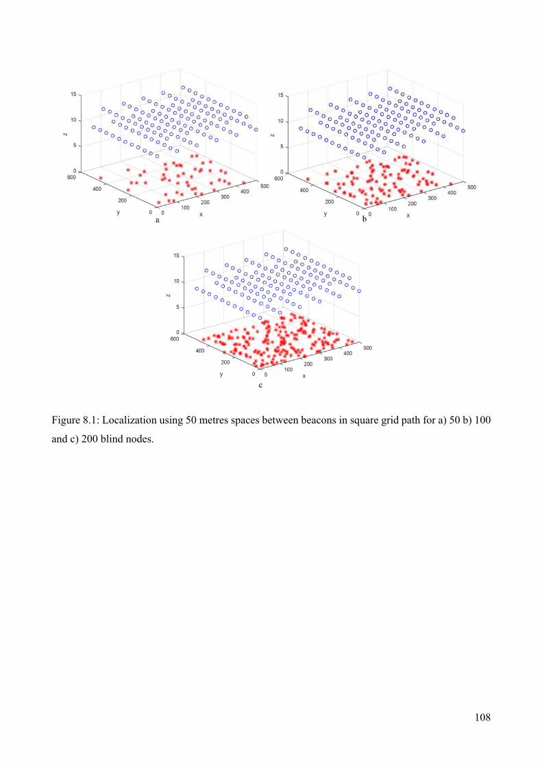
108
Figure 8.1: Localization using 50 metres spaces between beacons in square grid path for a) 50 b) 100
and c) 200 blind nodes.

109
Table 8.1: Positions of mobile anchor for square grid path.
Number x y z Number x y z Number x y z1 0 0 10 42 300 400 10 83 150 250 132 0 50 10 43 300 450 10 84 150 300 133 0 100 10 44 300 500 10 85 150 350 134 0 150 10 45 400 0 10 86 150 400 135 0 200 10 46 400 50 10 87 150 450 136 0 250 10 47 400 100 10 88 150 500 137 0 300 10 48 400 150 10 89 250 0 138 0 350 10 49 400 200 10 90 250 50 139 0 400 10 50 400 250 10 91 250 100 13
10 0 450 10 51 400 300 10 92 250 150 1311 0 500 10 52 400 350 10 93 250 200 1312 100 0 10 53 400 400 10 94 250 250 1313 100 50 10 54 400 450 10 95 250 300 1314 100 100 10 55 400 500 10 96 250 350 1315 100 150 10 56 500 0 10 97 250 400 1316 100 200 10 57 500 50 10 98 250 450 1317 100 250 10 58 500 100 10 99 250 500 1318 100 300 10 59 500 150 10 100 350 0 1319 100 350 10 60 500 200 10 101 350 50 1320 100 400 10 61 500 250 10 102 350 100 1321 100 450 10 62 500 300 10 103 350 150 1322 100 500 10 63 500 350 10 104 350 200 1323 200 0 10 64 500 400 10 105 350 250 1324 200 50 10 65 500 450 10 106 350 300 1325 200 100 10 66 500 500 10 107 350 350 1326 200 150 10 67 50 0 13 108 350 400 1327 200 200 10 68 50 50 13 109 350 450 1328 200 250 10 69 50 100 13 110 350 500 1329 200 300 10 70 50 150 13 111 450 0 1330 200 350 10 71 50 200 13 112 450 50 1331 200 400 10 72 50 250 13 113 450 100 1332 200 450 10 73 50 300 13 114 450 150 1333 200 500 10 74 50 350 13 115 450 200 1334 300 0 10 75 50 400 13 116 450 250 1335 300 50 10 76 50 450 13 117 450 300 1336 300 100 10 77 50 500 13 118 450 350 1337 300 150 10 78 150 0 13 119 450 400 1338 300 200 10 79 150 50 13 120 450 450 1339 300 250 10 80 150 100 13 121 450 500 1340 300 300 10 81 150 150 1341 300 350 10 82 150 200 13
Mobile anchor

110
8.2.2 Results Varying Node Density.
This first experiment uses 6 anchor positions (the minimum number of anchor positions identified
in Chapter 5 for reasonable accuracy), and varies node density between 50,100 and 200 blind nodes.
The blind nodes are localized within two generations (G1 to G2). For the first generation 35 out of
50 blind nodes could be localized (70%) using 6 mobile anchor positions only. These blind nodes
become the local anchors that can be used during the second generation. Figure 8.2 shows the
localization results. A complete table of localization error for each individual node is shown in
Appendix D. The highest median error during first generation (G1) is 20 metres for blind node 482,
336, 0 produced by 6 weak beacons from mobile anchor nodes. Another 12 nodes are localized during
the second generation (G2). However, there are another 3 blind nodes that could not be localized with
6 anchors. These nodes do not have any other nodes close enough to act as local anchors. Figure 8.3
shows the progress of localization generation by generation.
Figure 8.2: Median localization error for 50 blind nodes based on generation.
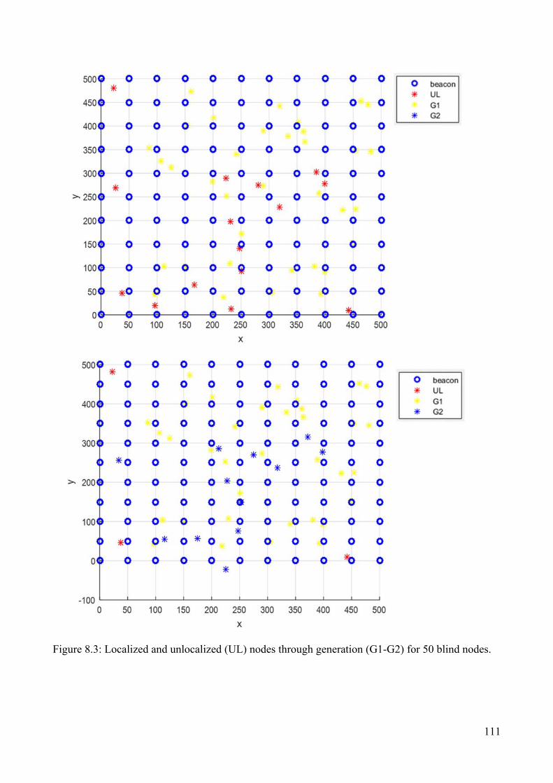
111
Figure 8.3: Localized and unlocalized (UL) nodes through generation (G1-G2) for 50 blind nodes.

112
Increasing the density of blind nodes from 50 to 100 or 200 blind nodes will make more local
anchors available, with higher (and more accurate) RSSI readings, hopefully assisting with
cooperative localization. Figure 8.4 shows the localization results for 100 nodes, with the complete
table of results in Appendix D.
Figure 8.4 shows the progress over 2 generations. The blind nodes are 78% successfully localized
during G1. Another 20 blind nodes are localized during the second generation. However, another 2
blind nodes are unable to localize due to lack of anchor positions unless we reduce the minimum
number of anchor positions to be used as shown in figure 8.5.
Figure 8.4: Average localization error for 100 blind nodes based on generation.

113
Figure 8.5: Localized and unlocalized (UL) nodes through generation (G1-G2) for 100 blind nodes.

114
For 200 blind nodes, all blind nodes have been completely localized after the second generation
using 6 anchor positions. Figure 8.7 shows the errors - most of the localization error for each of the
blind nodes are less than 20 metres. Figure 8.8 shows the G1 and G2 localized nodes.
The estimated position for both unlocalized blind nodes from the previous experiment (using 100
nodes) have been calculated during the second generation using additional local anchor 53, 419, 0
and 92, 458, 0 for blind node 22, 481, 0 while 114, 447,0 and 141, 417, 0 for blind node 166, 488, 0,
as shown in Table 8.2. These local anchors are part of the additional 100 nodes added for 200 blind
nodes. Additionally these local anchors are located close to the blind nodes and have stronger RSSI.
Therefore, it appears that a node density of 200 blind nodes is appropriate to reliably localize
randomly distributed blind nodes within a 500m x 500m sensing region, i.e. a density of 800 nodes
per square kilometre for our particular radio ranges. Table 8.3 summarises the results from the 3
scenarios in this experiment.
Figure 8.6: Average localization error for 200 blind nodes based on generation.

115
Table 8.2: Local and mobile anchor for localized blind node 13 and 42 by using 200 blind nodes.
Figure 8.7: Localized and unlocalized (UL) nodes through generation (G1-G2) for 200 blind nodes.
x y z x y z13 22 481 0 14.35 0 500 10 77 28
50 450 13 79 3250 500 13 83 42
0 450 10 88 5953 419 0 88 5992 458 0 90 68
42 166 488 0 11.40 150 500 13 74 23150 450 13 81 37200 450 10 84 45200 500 10 85 48114 447 0 86 51141 417 0 88 59
Blind node
Position Error (m) Local and Mobile anchor Path loss Est distance
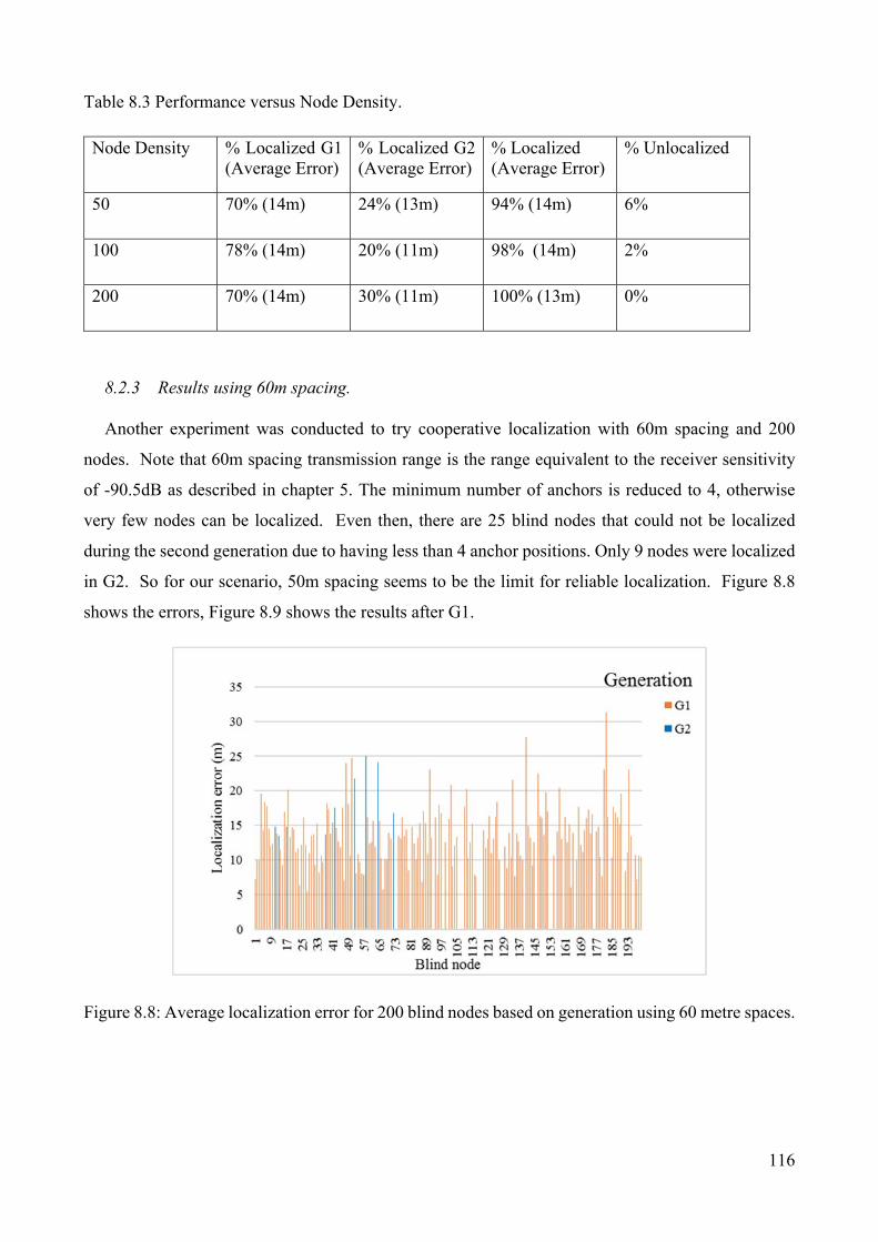
116
Table 8.3 Performance versus Node Density.
Node Density % Localized G1 (Average Error)
% Localized G2 (Average Error)
% Localized (Average Error)
% Unlocalized
50 70% (14m) 24% (13m) 94% (14m) 6%
100 78% (14m) 20% (11m) 98% (14m) 2%
200 70% (14m) 30% (11m) 100% (13m) 0%
8.2.3 Results using 60m spacing.
Another experiment was conducted to try cooperative localization with 60m spacing and 200
nodes. Note that 60m spacing transmission range is the range equivalent to the receiver sensitivity
of -90.5dB as described in chapter 5. The minimum number of anchors is reduced to 4, otherwise
very few nodes can be localized. Even then, there are 25 blind nodes that could not be localized
during the second generation due to having less than 4 anchor positions. Only 9 nodes were localized
in G2. So for our scenario, 50m spacing seems to be the limit for reliable localization. Figure 8.8
shows the errors, Figure 8.9 shows the results after G1.
Figure 8.8: Average localization error for 200 blind nodes based on generation using 60 metre spaces.

117
Figure 8.9: Localized and unlocalized (UL) nodes through generation (G1-G2) for 200 blind nodes
using 60 metre spaces.
8.2.4 Changing Minimum Number of Anchors.
The experiment is to identify how varying the minimum number of anchor positions used for
localizing 200 blind nodes affects the accuracy. More anchors should give a better initial estimate of
position, but may require more generations, and so this may lead to greater error propagation through
successive generations.
Three trials are done for 200 blind nodes, using a minimum of 6 or 7 or 8 anchors. Note that using
200 blind nodes gives adequate beacon density for some blind nodes to receive sufficient beacons.
As described in Chapter 5, 6 anchors is the minimum for good localization, and 7 or 8 will give better
accuracy. Figure 8.10 shows the errors for each of the 200 beacons for each generation. A minimum
of 6 anchors require two generations, 7 anchors require 3 generations, and 8 anchors require 5
generations.
Table 8.4 shows the average error across all the 200 blind nodes, both by generation, and in total.
The individual node results are given in Appendix E. The different generations for the 200 nodes and
6 anchors was shown previously in figure 8.9. The different generations for 7 and 8 anchors are
shown in figures 8.11 and 8.12. From these results there does not seem to be any significant reduction
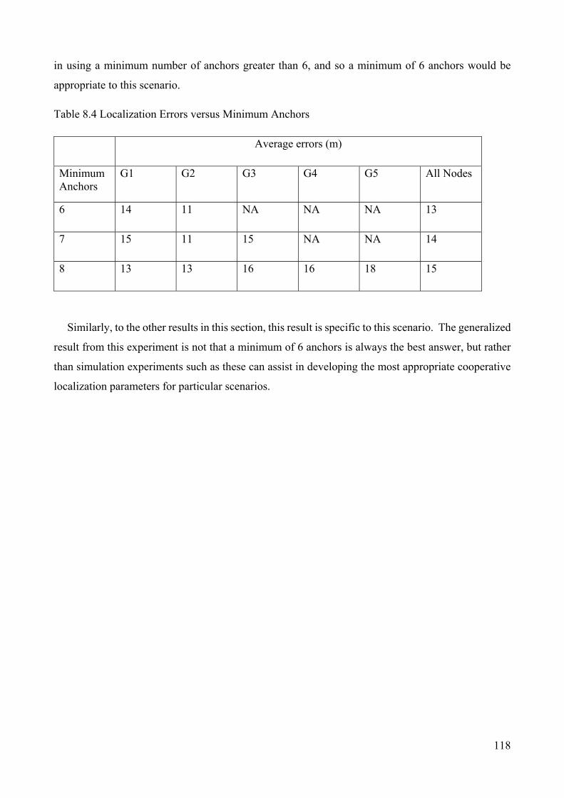
118
in using a minimum number of anchors greater than 6, and so a minimum of 6 anchors would be
appropriate to this scenario.
Table 8.4 Localization Errors versus Minimum Anchors
Average errors (m)
Minimum Anchors
G1 G2 G3 G4 G5 All Nodes
6 14 11 NA NA NA 13
7 15 11 15 NA NA 14
8 13 13 16 16 18 15
Similarly, to the other results in this section, this result is specific to this scenario. The generalized
result from this experiment is not that a minimum of 6 anchors is always the best answer, but rather
than simulation experiments such as these can assist in developing the most appropriate cooperative
localization parameters for particular scenarios.

119
(a)
(b)
(c)
Figure 8.10: Average localization error for 200 blind node based on generation using (a) 6, (b) 7 and (c) 8 minimum anchor positions.

120
Figure 8.11: Local anchors for each generation (G1 to G3) using 7 anchor positions.

121
Figure 8.12: Local anchors for each generation (G1 to G5) using 8 anchor positions.

122
8.3 Edge-Based Cooperative Localization.
8.3.1 Experimental Setup 2.
In this section, experiments are undertaken where a flight path attempts to localize blind nodes just
around the edges of the sensing area using a mobile anchor, and then to use cooperative localization
to progressively localize all the other nodes. The flight path consists of three loops at alternate 10m,
13m and 10m heights, with these loops spaced 50m apart, and the total length is 4.8km. Figure 8.13
shows the flight path and the 200 blind nodes. Table 8.5 lists the exact beacon positions. The
simulation is run for 40 iterations to determine the median error for all blind nodes. A minimum of 4
anchors are required for localization. The localization error and the number of generations will be
examined.
Starting with 200 blind nodes, the density of blind nodes will be increased until full localization
can be obtained.
Figure 8.13: Localization using 50 metres spacing between beacons using 200 blind nodes and edge
path planning.

123
Table 8.5: Position of mobile anchor node for edge path.
8.3.2 Results for 200 Blind Nodes.
Using edge path planning, many blind nodes around the edge of the area are localized by the
mobile anchor (G1) and the rest of the nodes around the edges are localized in G2. However, there
are insufficient local anchors (and no mobile anchors) for blind nodes in the central region to be
localized. The few central nodes that are localized have very high errors. Figure 8.14 shows the
localization errors for each of the nodes, and figure 8.15 shows the generations, including the large
unlocalized central region. The complete table is shown in appendix F. Those nodes located in the
centre of the sensing region could not be localized due to receiving less than 4 anchor positions.
By comparing the localization error of square grid path and edge path using 6 anchor positions to
localize 200 blind nodes, some of the blind nodes have higher error during the first generation (G1).
While the nodes localized during the second generation (G2) also have higher error with the
x y z x y z x y z1 0 0 10 41 350 0 10 81 100 100 102 0 50 10 42 400 0 10 82 100 150 103 0 100 10 43 450 0 10 83 100 200 104 0 150 10 44 500 0 10 84 100 250 105 0 200 10 45 50 50 13 85 100 300 106 0 250 10 46 50 100 13 86 100 350 107 0 300 10 47 50 150 13 87 100 400 108 0 350 10 48 50 200 13 88 100 400 109 0 400 10 49 50 250 13 89 150 400 10
10 0 450 10 50 50 300 13 90 200 400 1011 0 500 10 51 50 350 13 91 250 400 1012 0 500 10 52 50 400 13 92 300 400 1013 50 500 10 53 50 450 13 93 350 400 1014 100 500 10 54 50 450 13 94 400 400 1015 150 500 10 55 100 450 13 95 400 100 1016 200 500 10 56 150 450 13 96 400 150 1017 250 500 10 57 200 450 13 97 400 200 1018 300 500 10 58 250 450 13 98 400 250 1019 350 500 10 59 300 450 13 99 400 300 1020 400 500 10 60 350 450 13 100 400 350 1021 450 500 10 61 400 450 13 101 400 400 1022 500 500 10 62 450 450 13 102 100 100 1023 500 0 10 63 450 50 13 103 150 100 1024 500 50 10 64 450 100 13 104 200 100 1025 500 100 10 65 450 150 13 105 250 100 1026 500 150 10 66 450 200 13 106 300 100 1027 500 200 10 67 450 250 13 107 350 100 1028 500 250 10 68 450 300 13 108 400 100 10
Mobile anchorMobile anchor Mobile anchorNumber Number Number

124
maximum of 57 metres for node 207, 418, 0 due to weak RSSI which reached the maximum
sensitivity of -90.5dB. Blind node 31 (384, 264, 0) also has high error due to the error produced by
the local anchor of 430,245, 0 and 410, 307, 0 as stated in the following table.
Figure 8.14: Localization error for 200 blind nodes based on generations using edge path planning.
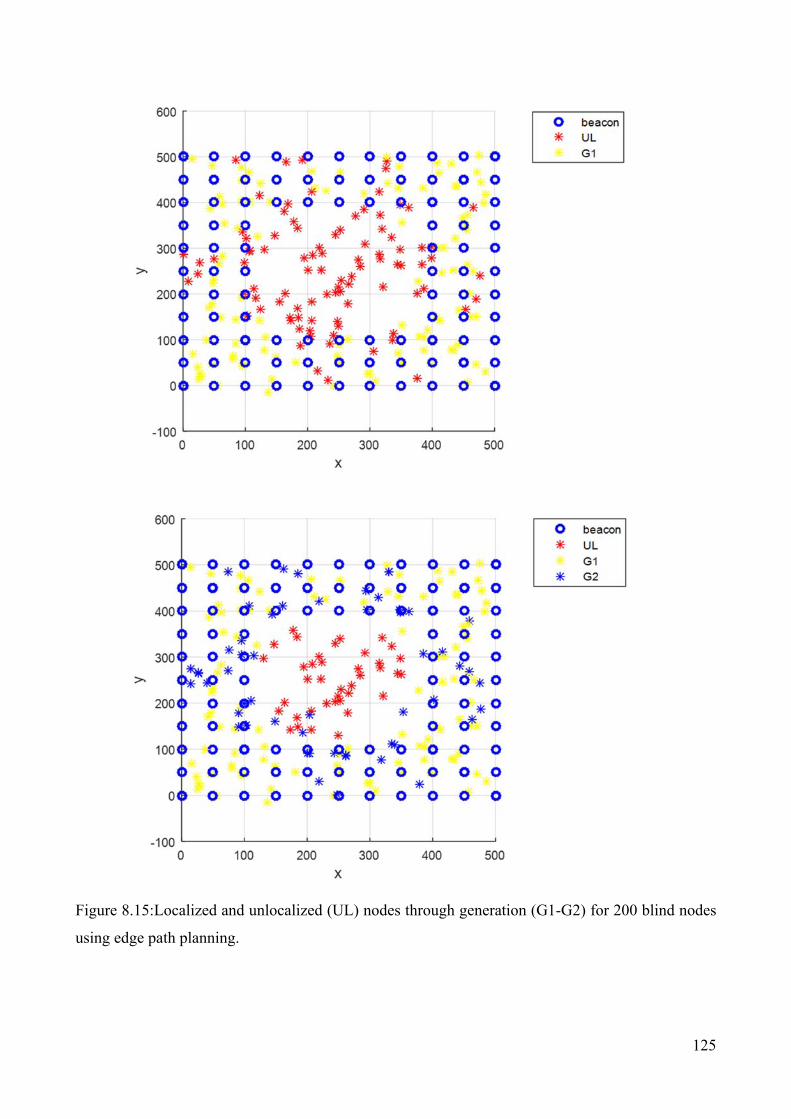
125
Figure 8.15:Localized and unlocalized (UL) nodes through generation (G1-G2) for 200 blind nodes
using edge path planning.

126
8.3.3 Results for 1000 Blind Nodes.
As shown in figure 8.16, there were many blind nodes located in the centre of the sensing region
that could not be localized using the edge path planning. This is because there was an insufficient
density of local anchors to propagate localization into this region.
Therefore, additional blind nodes are added to increase the chances of localization by local
anchors. For 500 nodes, full localization was still not possible. The number of blind nodes is increased
to 1000 nodes as shown in figure 8.16. For this very large simulation, faster DML localization was
used to reduce the very long simulation time (remembering that the whole simulation is run 40 times
to get stable statistics).
With this setup, all blind nodes are fully localized after the fourth generation as in figure 8.17.
Figure 8.16: Localization for 1000 blind nodes using edge path planning.
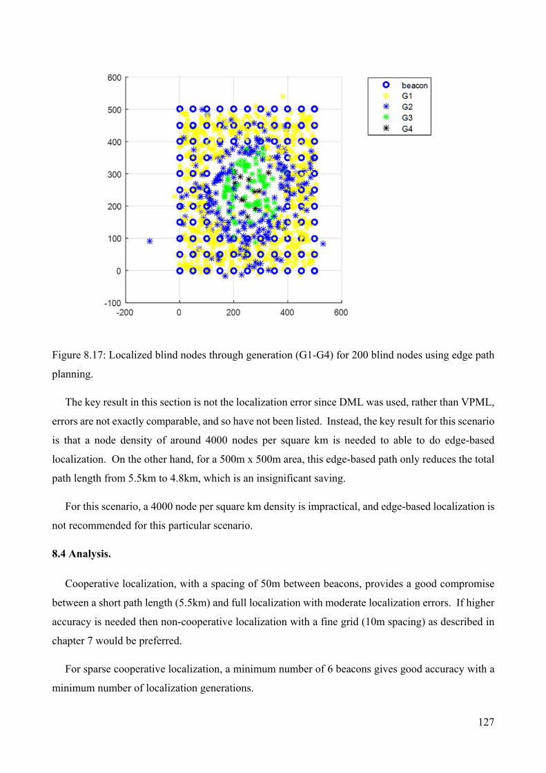
127
Figure 8.17: Localized blind nodes through generation (G1-G4) for 200 blind nodes using edge path
planning.
The key result in this section is not the localization error since DML was used, rather than VPML,
errors are not exactly comparable, and so have not been listed. Instead, the key result for this scenario
is that a node density of around 4000 nodes per square km is needed to able to do edge-based
localization. On the other hand, for a 500m x 500m area, this edge-based path only reduces the total
path length from 5.5km to 4.8km, which is an insignificant saving.
For this scenario, a 4000 node per square km density is impractical, and edge-based localization is
not recommended for this particular scenario.
8.4 Analysis.
Cooperative localization, with a spacing of 50m between beacons, provides a good compromise
between a short path length (5.5km) and full localization with moderate localization errors. If higher
accuracy is needed then non-cooperative localization with a fine grid (10m spacing) as described in
chapter 7 would be preferred.
For sparse cooperative localization, a minimum number of 6 beacons gives good accuracy with a
minimum number of localization generations.
128
Edge-based path planning can use localize a ring around the edge of the sensing area, but in order
for this localization to propagate into a central area with no mobile beacon messages, an impractically
high node density is required
This thesis only presents an initial investigation into cooperative localization, which shows the
general performance of the techniques when there are insufficient mobile anchor nodes for direct
localization. For the purposes of this investigation, the same 3-D PDF of range versus RSSI is used
in all cases. In both the case of the mobile anchor beacons, and the cooperative sensor node beacons,
only the errors in range are considered in the PDF. In practice, these PDFs could also consider errors
in the GPS position of the mobile beacon, and the errors in the estimated sensor node anchor positions.
However, this work is outside the scope of this thesis, and is left for future work.
All these results are specific to this particular scenario, and radio range characteristics, and the
results do not transfer to general guidelines. Rather, the key contribution is that such simulation
studies can provide relatively quick decisions about operational requirements for the use of a mobile
anchor prior to deployment.
The next chapter will summarize the findings and contributions from all the research questions.
The possible directions for future research are also being discussed in the end of chapter 9.

129
CHAPTER 9
CONCLUSION, CONTRIBUTIONS AND FUTURE WORK
This thesis has examined a number of research questions about RSSI-based localization of wireless
sensor nodes, with particular reference to a motivating scenario of air-dropped sensors which are
localized using an airborne mobile anchor.
The studies make extensive use of stochastic simulations to investigate the expected performance
of different algorithms. A preliminary outdoor experiment as described in Chapter 4 was undertaken
to validate the proposed radio propagation model, and to identify the parameters for Matlab
simulation. Specifically the parameters of nominal path loss , the log normal shadowing power n
and the standard deviation of path loss were estimated.
This conclusions chapter consists of three parts. Sections 9.1, 9.2, 9.3 and 9.4 summarize the
answers to the four research questions posed in Chapter 3. Section 9.5 summarizes the key original
contributions. Section 9.6 proposes directions for future work.
9.1 Research Question 1 (Localization accuracy vs. number of mobile anchor positions).
RQ1: How does the localization performance of a mobile anchor vary with different numbers of beacon packets, and how does it compare with the use of fixed anchors, or combinations of fixed and mobile anchors?
A deterministic multilateration algorithm (DML) was simulated to uncover detailed performance
analysis of different scenarios, which explored the impact on localization error of random and
designated positions of mobile anchor nodes, and different numbers of nodes.
It was found that localization accuracy varies with the number of mobile anchor node positions
used for multilateration in a non-monotonic fashion. In other words, more anchors are not always
better. As a guideline, between 6 to 13 anchor readings gives the best compromise between the
reduction of errors from more readings and the increase in solution error by including low RSSI
values (i.e. less accurate range estimates).
The localization accuracy depends strongly on the position of the geometric arrangement of mobile
anchor node points. The best anchors are not necessarily the closest anchors. Therefore, anchor
geometry is important.

130
The localization performance was not significantly improved by adding some fixed anchor points
at ground level, and the remainder of the experiments only considered a mobile anchor.
Therefore, the new probabilistic algorithm has been introduced to improve the localization
performance compared to the DML algorithm.
9.2 Research Question 2 (Probabilistic Multilateration).
RQ2: What is the localization performance of probabilistic localization algorithms compared to
deterministic algorithms, and how does this vary with the number of beacon packets?
I developed a new formulation called Volume Probabilistic Multilateration localization (VPML)
using gradient descent optimization, and compared it with previously published techniques of Linear
Probabilistic Multilateration (LPML) and Deterministic Multilateration (DML).
Our analysis shows that VPML performs better than DML and LPML and the localization error is
reduced by up to 75% compared to commonly used DML. Approximately 6 to 12 RSSI readings are
suggested for best localization performance.
However, the localization performance using this algorithm can be improved by analysing the
impact of geometric sensitivity of beacon positions and mobile anchor trajectories as in research
question 3.
9.3 Research Question 3 (Geometric sensitivity and trajectory of mobile anchor node).
RQ3: How does the mobile anchor node’s trajectory influence the performance and what is the
most suitable trajectory based on the proposed scenario? How does performance vary with the
number of beacons sent and the positions that they are sent from?
The investigation of the geometric arrangement of beacon positions shows that it is better to choose
“well-positioned” beacon positions, not just those with highest RSSI. So while a very dense array of
beacons (e.g. using a 5m grid of beacons) gives many beacons, this does not improve localization
accuracy.
Specifically for this scenario, I propose that the mobile anchor should travel using the square grid
path with height diversity (alternate 10 metres height lower path and 13 metres upper path). The best
accuracy is with a spacing between beacons of 10 metres. Spacing above 30m do not allow all nodes
to be localized.
These experimental results are specific to this scenario, but they do demonstrate that localization of
air-dropped sensors using an airborne mobile anchor is feasible, and that simulation experiments can

131
suggest suitable operational parameters for that localization. Furthermore, the results show that VPML
gives significantly better localization accuracy compare to previous techniques.
Furthermore, the work for geometric sensitivity and mobile anchor trajectories can be enhanced
using the cooperative localization to localize any blind nodes with insufficient beacon packets. Also,
cooperative localization can reduce the travel distance of the mobile anchor to trade-off between the
energy expended and localization accuracy.
9.4 Research Question 4 (Cooperative localization).
RQ4: What is the relative localization performance of adding inter-blind node range estimates to
anchor range estimates?
The previous experiments in chapter 7 showed that widely spaced beacons do not allow all nodes
to be localized. Thus, experiments in Chapter 8 demonstrated that cooperative localization can
improve localization performance.
The localization of blind nodes through several generations of cooperative localization based on a
50 metres beacon spacing showed full node localization, acceptable localization accuracy, and
significantly reduced path length. Such cooperative localization needs reasonable node density – 800
nodes per square kilometre in this scenario.
However, edge-based path planning was less successful. An impractically high node density (4000
nodes per square kilometre) and 4 generations were required.
9.5 Original Contributions.
The most significant contribution of the thesis is the development of the new VPML localization
technique, and the demonstration of its superior performance compared to previous deterministic and
probabilistic multilateration techniques.
At least at simulation level, the research has demonstrated the feasibility of the localization of a
sensor field using an airborne mobile anchor and this new VPML algorithm, and has examined how
stochastic simulation can be used to establish practical operational parameters that are likely to lead
to the best localization performance.
The thesis has identified that the geometric arrangement of airborne beacons has a significant
impact of localization performance.

132
Finally, the thesis has shown that cooperative localization is a useful technique to deal with a small
percentage of unlocalized nodes, but is not practical for localizing nodes in areas without any mobile
beacon messages.
9.6 Future Research.
There are many possible directions to extend this current work on sensor localization algorithms.
Future work could usefully include the beacon position uncertainty caused by GPS. This work
assumes “exact” beacon positions. The effect on localization from beacon position inaccuracy would
be a useful next step to pursue.
The thesis has identified the impact of beacon geometry on accuracy, and informally identified
that inter-beacon ray angles around 90 degrees do improve accuracy. Future work could identify how
to select the “best” beacons from those available.
Our localization algorithms are currently written in MATLAB, and with little regard to
computational efficiency. To facilitate their application to real implementations, the VPML
algorithm should be recoded in a computationally efficient language such as C. This is especially
true if the implementation was required to be a distributed computing implementation on the sensor
nodes themselves.
Finally, field experiments with real nodes, real mobile anchors and real distributed algorithms
would be an obvious next step. Unfortunately, the cost and logistics of running such experiments
was outside the scope of this PhD project, but hopefully these results have shown that such
experiments would be useful and worthwhile.

133
References
[1] N. A. Alrajeh, M. Bashir, and B. Shams, "Localization techniques in wireless sensor
networks," International Journal of Distributed Sensor Networks, vol. 9, no. 6, pp. 1-9, 2013.
DOI: 10.1155/2013/304628
[2] P. Corke, T. Wark, R. Jurdak, W. Hu, P. Valencia, and D. Moore, "Environmental wireless
sensor networks," Proceedings of the IEEE, vol. 98, no. 11, pp. 1903-1917, 2010. DOI:
10.1109/JPROC.2010.2068530
[3] T. Wark et al., "Springbrook: Challenges in developing a long-term, rainforest wireless sensor
network," in International Conference on Intelligent Sensors, Sensor Networks and
Information Processing, 2008. ISSNIP 2008. , pp. 599-604: IEEE. 2008, DOI:
10.1109/ISSNIP.2008.4762055
[4] P. Pounds, T. Potie, F. Kendoul, S. Singh, R. Jurdak, and J. Roberts, "Automatic distribution
of disposable self-deploying sensor modules," in Experimental Robotics, pp. 535-543. 2016,
DOI: 10.1007/978-3-319-23778-7_35
[5] I. Ahmad, "Localization of wireless sensor networks using a mobile beacon," in Pervasive
Computing and Communication Workshops (PerCom Workshops), 2016 IEEE International
Conference on, pp. 1-3: IEEE. 2016, DOI: 10.1109/PERCOMW.2016.7457081
[6] E. M. García, A. Bermúdez, and R. Casado, "Range-free localization for air-dropped WSNs
by filtering node estimation improvements," in IEEE 6th International Conference Wireless
and Mobile Computing, Networking and Communications (WiMob), pp. 471-478: IEEE.
2010, DOI: 10.1109/WIMOB.2010.5645023
[7] H. Patel and N. Pandya, "3D localization algorithms for wireless sensor networks," IOSR
Journal of Computer Engineering (IOSR-JCE), vol. 12, no. 1, pp. 61-66, 2013. DOI:
10.6084/M9.FIGSHARE.1104171
[8] O. Chia-Ho and S. Kuo-Feng, "Sensor position determination with flying anchors in three-
dimensional wireless sensor networks," IEEE Transactions on Mobile Computing, vol. 7, no.
9, pp. 1084-1097, 2008. DOI: 10.1109/tmc.2008.39
[9] R. Kumar, S. Kumar, D. Shukla, R. S. Raw, and O. Kaiwartya, "Geometrical localization
algorithm for three dimensional wireless sensor networks," Wireless Personal
Communications, vol. 79, no. 1, pp. 249-264, 2014. DOI: 10.1007/s11277-014-1852-6
[10] V. Yadav, M. K. Mishra, A. Sngh, and M. Gore, "Localization scheme for three dimensional
wireless sensor networks using GPS enabled mobile sensor nodes," International Journal of

134
Next-Generation Networks (IJNGN), vol. 1, no. 1, pp. 60-72, 2009.
http://airccse.org/journal/ijngn/papers/8.pdf
[11] H. Seo and H. Kim, "Four anchor sensor nodes based localization algorithm over three-
dimensional space," Journal of Information and Communication Convergence Engineering,
vol. 10, no. 4, pp. 349-358, 2012. DOI: 10.6109/jicce.2012.10.4.349
[12] Y. J. Fu, T. H. Lee, L. H. Chang, and T. P. Wang, "A single mobile anchor localization scheme
for wireless sensor networks," in IEEE 13th International Conference pp. 946-950: IEEE.
2011, DOI: 10.1109/ChiCC.2016.7554631
[13] F. Abdi and A. T. Haghighat, "A hybrid RSSI based localization algorithm for WSN using a
mobile anchor node," in International Conference on Computing, Communication and
Networking Technologies (ICCCNT) pp. 1-6: IEEE. 2014, DOI:
10.1109/ICCCNT.2014.6963058
[14] J. K. Hedrick, B. Basso, J. Love, and B. M. Lavis, "Tools and techniques for mobile sensor
network control," Journal of Dynamic Systems, Measurement, and Control, vol. 133, no. 2,
pp. 1-11, 2011. DOI: 10.1115/1.4003369
[15] I. Amundson and X. D. Koutsoukos, "A survey on localization for mobile wireless sensor
networks," in Mobile Entity Localization and Tracking in GPS-less Environnments: Springer,
pp. 235-254, 2009, DOI: 10.1.1.156.8358.
[16] T. Ahmad, X. J. Li, and B.-C. Seet, "3D localization based on parametric loop division and
subdivision surfaces for wireless sensor networks," in Wireless and Optical Communication
Conference (WOCC), pp. 1-6: IEEE. 2016, DOI: 10.1109/WOCC.2016.7506540
[17] A. Kumar, "Optimized range-free 3D node localization in wireless sensor networks using
firefly algorithm," in International Conference on Signal Processing and Communication
(ICSC), pp. 14-19: IEEE. 2015, DOI: 10.1109/ICSPCom.2015.7150611
[18] S. Lee and K. Kim, "Localization with a mobile beacon in underwater acoustic sensor
networks," Sensors, vol. 12, no. 5, pp. 5486-5501, 2012. DOI: 10.1109/EUC.2010.52
[19] E. Guerrero, J. Alvarez, and L. Rivero, "3D-ADAL: A three-dimensional distributed range-
free localization algorithm for wireless sensor networks based on unmanned aerial vehicles,"
in Fifth International Conference on Digital Information Management (ICDIM), pp. 332-338:
IEEE. 2010, DOI: 10.1109/ICDIM.2010.5664253
[20] L. Karim, N. Nasser, and T. El Salti, "RELMA: a range free localization approach using
mobile anchor node for wireless sensor networks," in Global Telecommunications Conference
pp. 1-5: IEEE. 2010, DOI: 10.1109/GLOCOM.2010.5683802
135
[21] N. Bulusu, J. Heidemann, and D. Estrin, "GPS-less low-cost outdoor localization for very
small devices," IEEE Personal Communications, vol. 7, no. 5, pp. 28-34, 2000. DOI:
10.1109/98.878533
[22] S. Feng, C.-d. Wu, Y.-z. Zhang, and Z.-x. Jia, "Grid-Based Improved Maximum Likelihood
Estimation for Dynamic Localization of Mobile Robots," International Journal of Distributed
Sensor Networks, vol. 10, no. 3, pp. 1-16, 2014. DOI: 10.1155/2014/271547
[23] D. Niculescu and B. Nath, "Ad hoc positioning system (APS)," in Global Telecommunications
Conference, 2001. GLOBECOM'01. IEEE, vol. 5, pp. 2926-2931: IEEE. 2001, DOI:
10.1109/GLOCOM.2001.965964
[24] A. Kulaib, R. Shubair, M. Al-Qutayri, and J. W. Ng, "Improved DV-hop localization using
node repositioning and clustering," in International Conference on Communications, Signal
Processing, and their Applications (ICCSPA), pp. 1-6: IEEE. 2015, DOI:
10.1109/ICCSPA.2015.7081314
[25] A. Karbasi and S. Oh, "Distributed sensor network localization from local connectivity:
Performance analysis for the HOP-TERRAIN algorithm," in ACM SIGMETRICS
Performance Evaluation Review, vol. 38, no. 1, pp. 61-70: ACM. 2010, DOI:
10.1145/1811099.1811047
[26] W. Cheng, J. Li, and H. Li, "An improved APIT location algorithm for wireless sensor
networks," in Advances in Electrical Engineering and Automation: Springer, pp. 113-119,
2012, DOI: 10.1007/978-3-642-27951-5_17.
[27] A. Mesmoudi, M. Feham, and N. Labraoui, "Wireless sensor networks localization
algorithms: A comprehensive survey," International Journal of Computer Networks &
Communications, vol. 5, no. 6, pp. 45-64, 2013. DOI: 10.5121/ijcnc.2013.5603
[28] G. Han, H. Xu, T. Q. Duong, J. Jiang, and T. Hara, "Localization algorithms of wireless sensor
networks: A survey," Telecommunication Systems, pp. 1-18, 2013. DOI: 10.1007/s11235-
011-9564-7
[29] G. Han, D. Choi, and W. Lim, "Reference node selection algorithm based on trilateration and
performance analysis in indoor sensor networks," in IEEE International Conference on
Intelligent Computer Communication and Processing, pp. 177-184: IEEE. 2007, DOI:
10.1109/ICCP.2007.4352158
[30] G. Han, C. Zhang, J. Lloret, L. Shu, and J. J. Rodrigues, "A mobile anchor assisted localization
algorithm based on regular hexagon in wireless sensor networks," Scientific World Journal,
vol. 2014, pp. 1-13, 2014. DOI: 10.1155/2014/219371
136
[31] C. Seow, W. K. Seah, and Z. Liu, "Hybrid mobile wireless sensor network cooperative
localization," in IEEE 22nd International Symposium on Intelligent Control, pp. 29-34: IEEE.
2007, DOI: 10.1109/ISIC.2007.4450856
[32] F. Hammer et al., "Performance Evaluation of 3D-Position Estimation Systems," IEEE
Sensors Journal, vol. 16, no. 16, pp. 6416-6424, 2016. DOI: 10.1109/jsen.2016.2581489
[33] I. F. Akyildiz, W. Su, Y. Sankarasubramaniam, and E. Cayirci, "Wireless sensor networks: A
survey," Computer Networks, vol. 38, no. 4, pp. 393-422, 2002. DOI: 10.1016/S1389-
1286(01)00302-4
[34] R. Kaune, "Accuracy studies for TDOA and TOA localization," in International Conference
on Information Fusion (FUSION), pp. 408-415: IEEE. 2012,
http://xplorestaging.ieee.org/servlet/opac?punumber=6269381
[35] G. Mao, B. Fidan, and B. D. O. Anderson, "Wireless sensor network localization techniques,"
Computer Networks, vol. 51, no. 10, pp. 2529-2553, 2007. DOI:
10.1016/j.comnet.2006.11.018
[36] B. J. Dil and P. J. Havinga, "RSS-based localization with different antenna orientations," in
AustralasianTelecommunication Networks and Applications Conference (ATNAC), pp. 13-18:
IEEE. 2010, DOI: 10.1109/ATNAC.2010.5679581
[37] N. A. Dieng, C. Chaudet, M. Charbit, L. Toutain, and T. B. Meriem, "Experiments on the
RSSI as a range estimator for indoor localization," in International Conference on New
Technologies, Mobility and Security (NTMS), , pp. 1-5: IEEE. 2012, DOI:
10.1109/NTMS.2012.6208722
[38] O. G. Adewumi, K. Djouani, and A. M. Kurien, "RSSI based indoor and outdoor distance
estimation for localization in WSN," in IEEE International Conference on Industrial
Technology (ICIT), pp. 1534-1539: IEEE. 2013, DOI: 10.1109/ICIT.2013.6505900
[39] J. Xu, W. Liu, F. Lang, Y. Zhang, and C. Wang, "Distance measurement model based on RSSI
in WSN," Wireless Sensor Network, vol. 2, no. 8, pp. 606-611, 2010. DOI:
10.4236/wsn.2010.28072
[40] R. Peng and M. L. Sichitiu, "Robust, probabilistic, constraint-based localization for wireless
sensor networks," in SECON, pp. 541-550. 2005, DOI: 10.1109/SAHCN.2005.1557106
[41] M. L. Sichitiu, V. Ramadurai, and P. Peddabachagari, "Simple algorithm for outdoor
localization of wireless sensor networks with inaccurate range measurements," in
International Conference on Wireless Networks, vol. 2003, pp. 1-7. 2003, DOI: 10.1.1.3.8399
[42] S. Kotwal, S. Nigam, S. Verma, and R. Abrol, "Multi hop multi anchor geometrical
computation based localization algorithm for wireless sensor networks with limited

137
communication," in IEEE Conference on Wireless Communication and Sensor Networks
(WCSN), pp. 1-6: IEEE. 2009, DOI: 10.1109/WCSN.2009.5434804
[43] G. Zanca, F. Zorzi, A. Zanella, and M. Zorzi, "Experimental comparison of RSSI-based
localization algorithms for indoor wireless sensor networks," in Real-World Wireless Sensor
Networks, pp. 1-5: ACM. 2008, DOI: 10.1145/1435473.1435475
[44] G. Blumrosen, B. Hod, T. Anker, D. Dolev, and B. Rubinsky, "Enhancing RSSI-based
tracking accuracy in wireless sensor networks," ACM Transactions on Sensor Networks, vol.
9, no. 3, pp. 1-28, 2013. DOI: 10.1145/2480730.2480732
[45] M. Fanourakis and K. Wac, "ReNLoc: An anchor-free localization algorithm for indirect
ranging," in IEEE International Symposium on a World of Wireless, Mobile and Multimedia
Networks (WoWMoM), pp. 1-9: IEEE. 2015, DOI: 10.1109/WoWMoM.2015.7158145
[46] K. F. Taraktas, O. Ceylan, and B. Yagci, "Received signal strength technique performance in
sensor network localization application," in International Conference on Broadband, Wireless
Computing, Communication and Applications (BWCCA), pp. 357-362: IEEE. 2010, DOI:
10.1109/BWCCA.2010.96.357
[47] P. Kułakowski, J. Vales-Alonso, E. Egea-López, W. Ludwin, and J. García-Haro, "Angle-of-
arrival localization based on antenna arrays for wireless sensor networks," Computers &
Electrical Engineering, vol. 36, no. 6, pp. 1181-1186, 2010. DOI:
10.1016/j.compeleceng.2010.03.007
[48] A. V. Tondwalkar and P. Vinayakray-Jani, "Terrestrial localization by using Angle of Arrival
measurements in wireless sensor network," in 2015 International Conference on
Computational Intelligence and Communication Networks (CICN), pp. 188-191: IEEE. 2015,
DOI: 10.1109/CICN.2015.44
[49] S. Tomic, M. Beko, R. Dinis, and L. Berbakov, "Cooperative localization in wireless sensor
networks using combined measurements," in 23rd Telecommunications Forum Telfor
(TELFOR), pp. 488-491: IEEE. 2015, DOI: 10.1186/1687-1499-2011-72
[50] S. Tomic, M. Beko, and R. Dinis, "3-D target localization in wireless sensor networks using
RSS and AoA measurements," IEEE Transactions on Vehicular Technology, vol. 66, no. 4,
pp. 3197-3210, 2017. DOI: 10.1109/tvt.2016.2589923
[51] S. Wang, B. R. Jackson, and R. Inkol, "Hybrid RSS/AOA emitter location estimation based
on least squares and maximum likelihood criteria," in Biennial Symposium on
Communications (QBSC), pp. 24-29: IEEE. 2012, DOI: 10.1109/QBSC.2012.6221344
[52] L. Gazzah, L. Najjar, and H. Besbes, "Geometrical positioning with selective hybrid
RSSD/AOA weighting AML algorithm for NLOS localization," in International Conference

138
on Multimedia Computing and Systems (ICMCS), pp. 740-745: IEEE. 2014, DOI:
10.1109/ICMCS.2014.6911189
[53] S. M. M. Dehghan and H. Moradi, "A multi-step Gaussian filtering approach to reduce the
effect of non-Gaussian distribution in aerial localization of an RF source in NLOS condition,"
in RSI/ISM International Conference on Robotics and Mechatronics (ICRoM), pp. 43-48:
IEEE. 2013, DOI: 10.1109/ICRoM.2013.6510079
[54] G. Blewitt, "Basics of the GPS technique: observation equations," Geodetic Applications of
GPS, pp. 10-54, 1997. DOI: 10.1.1.570.6440
[55] Y. Yun, J. Jin, N. Kim, J. Yoon, and C. Kim, "Outdoor localization with optical navigation
sensor, IMU and GPS," in IEEE Conference on Multisensor Fusion and Integration for
Intelligent Systems (MFI), pp. 377-382: IEEE. 2012, DOI: 10.1109/MFI.2012.6343007
[56] Q. D. Vo and P. De, "A survey of fingerprint-based outdoor localization," IEEE
Communications Surveys & Tutorials, vol. 18, no. 1, pp. 491-506, 2016. DOI:
10.1109/COMST.2015.2448632
[57] X. Wang, O. Bischoff, R. Laur, and S. Paul, "Localization in wireless ad-hoc sensor networks
using multilateration with RSSI for logistic applications," Procedia Chemistry, vol. 1, no. 1,
pp. 461-464, 2009. DOI: 10.1016/j.proche.2009.07.115
[58] A. Moragrega and C. Ibars, "Performance analysis of cooperative and range based localization
algorithms for Zigbee and 802.15.4a wireless sensor networks," in IEEE International
Symposium on Personal Indoor and Mobile Radio Communications (PIMRC), pp. 1996-2001:
IEEE. 2010, DOI: 10.1109/PIMRC.2010.5671594
[59] S. Rai B and S. Varma, "An algorithmic approach to wireless sensor networks localization
using rigid graphs," Journal of Sensors, vol. 2016, pp. 1-11, 2016. DOI:
10.1155/2016/3986321
[60] A. Pal, "Localization algorithms in wireless sensor networks: Current approaches and future
challenges," Network Protocols and Algorithms, vol. 2, no. 1, pp. 45-73, 2010. DOI:
10.5296/npa.v2i1.279
[61] B. Dawes and K.-W. Chin, "A comparison of deterministic and probabilistic methods for
indoor localization," Journal of Systems and Software, vol. 84, no. 3, pp. 442-451, 2011. DOI:
10.1016/j.jss.2010.11.888
[62] S. Ruder, "An overview of gradient descent optimization algorithms," arXiv preprint
arXiv:1609.04747, 2016. DOI: 10.1109/ICDAR.2011.95
[63] R. Garg, A. L. Varna, and M. Wu, "Gradient descent approach for secure localization in
resource constrained wireless sensor networks," in IEEE International Conference on
139
Acoustics Speech and Signal Processing (ICASSP), pp. 1854-1857: IEEE. 2010, DOI:
10.1109/ICASSP.2010.5495371
[64] C. Müller, D. I. Alves, B. F. Uchôa-Filho, R. Machado, J. B. S. Martins, and L. L. de Oliveira,
"Improved solution for node location multilateration algorithms in wireless sensor networks,"
Electronics Letters, vol. 52, no. 13, pp. 1179-1181, 2016. DOI: 10.1049/el.2016.0688
[65] N. A. Alwan and A. S. Mahmood, "Distributed gradient descent localization in wireless sensor
networks," Arabian Journal for Science and Engineering, vol. 40, no. 3, pp. 893-899, 2015.
DOI: 10.1007/s13369-014-1552-2
[66] B. Tatham and T. Kunz, "Anchor node placement for localization in wireless sensor
networks," in International Conference on Wireless and Mobile Computing, Networking and
Communications (WiMob), pp. 180-187: IEEE. 2011, DOI: 10.1109/WiMOB.2011.6085407
[67] R. Akl, K. Pasupathy, and M. Haidar, "Anchor nodes placement for effective passive
localization," in International Conference on Selected Topics in Mobile and Wireless
Networking (iCOST), pp. 127-132: IEEE. 2011, DOI: 10.1109/iCOST.2011.6085823
[68] S. Lee, E. Kim, C. Kim, and K. Kim, "Localization with a mobile beacon based on geometric
constraints in wireless sensor networks," IEEE Transactions on Wireless Communications,
vol. 8, no. 12, pp. 5801-5805, 2009. DOI: 10.1109/twc.2009.12.090319
[69] P. Moravek, D. Komosny, M. Simek, and J. Muller, "Multilateration and flip ambiguity
mitigation in ad-hoc networks," Przeglad Elektrotechniczny (Electrical Review), vol. 88, no.
5b, pp. 222-229, 2012. http://pe.org.pl/articles/2012/5b/50.pdf
[70] S. Han, J. Yue, W. Meng, and C. Li, "A novel flip ambiguities detection algorithm for WSN
localization," in IEEE Globecom Workshops (GC Wkshps), pp. 1-6: IEEE. 2015, DOI:
10.1109/GLOCOMW.2015.7413981
[71] C. Alippi and G. Vanini, "A RSSI-based and calibrated centralized localization technique for
wireless sensor networks," in Fourth Annual IEEE International Conference on Pervasive
Computing and Communications Workshops, pp. 5 pp.-305: IEEE. 2006, DOI:
10.1109/PERCOMW.2006.13
[72] H.-S. Ahn and W. Yu, Indoor localization techniques based on wireless sensor networks.
INTECH Open Access Publisher, 2009, DOI: 10.5772/6998.
[73] W.-H. Kuo, Y.-S. Chen, K.-T. Cheng, and T.-W. Lu, "Signal strength based indoor and
outdoor localization scheme in zigbee sensor networks," IAENG International Journal of
Computer Science, vol. 23, no. 1, 2016.
http://www.iaeng.org/IJCS/issues_v43/issue_1/IJCS_43_1_07.pdf
140
[74] S. P. Singh and S. C. Sharma, "Range Free Localization Techniques in Wireless Sensor
Networks: A Review," Procedia Computer Science, vol. 57, pp. 7-16, 2015. DOI:
10.1016/j.procs.2015.07.357
[75] T. Zhang, J. He, and H. Yu, "Secure localization in wireless sensor networks with mobile
beacons," International Journal of Distributed Sensor Networks, vol. 2012, pp. 1-11, 2012.
DOI: 10.1155/2012/732381
[76] G. Teng, K. Zheng, and W. Dong, "Adapting mobile beacon-assisted localization in wireless
sensor networks," Sensors, vol. 9, no. 4, pp. 2760-2779, 2009. DOI: 10.3390/s90402760
[77] K. Kim and W. Lee, "MBAL: A mobile beacon-assisted localization scheme for wireless
sensor networks," in Proceedings of 16th International Conference on Computer
Communications and Networks ICCCN pp. 57-62: IEEE. 2007, DOI:
10.1109/ICCCN.2007.4317797
[78] N. B. Priyantha, H. Balakrishnan, E. D. Demaine, and S. Teller, "Mobile-assisted localization
in wireless sensor networks," in Annual Joint Conference of the IEEE Computer and
Communications Societies INFOCOM, vol. 1, pp. 172-183: IEEE. 2005, DOI:
10.1109/INFCOM.2005.1497889
[79] C.-H. Ou, "A localization scheme for wireless sensor networks using mobile anchors with
directional antennas," IEEE Sensors Journal, vol. 11, no. 7, pp. 1607-1616, 2011. DOI:
10.1109/JSEN.2010.2102748
[80] W.-H. Liao, Y.-C. Lee, and S. P. Kedia, "Mobile anchor positioning for wireless sensor
networks," IET Communications, vol. 5, no. 7, pp. 914-921, 2011. DOI: 10.1049/iet-
com.2010.0336
[81] O. Artemenko, A. Rubina, T. Simon, and A. Mitschele-Thiel, "Evaluation of different static
trajectories for the localization of users in a mixed indoor-outdoor scenario using a real
unmanned aerial vehicle," in International Conference on Ad Hoc Networks, pp. 123-133:
Springer. 2015, DOI: 10.1007/978-3-319-25067-0_10
[82] K. F. Ssu, C. H. Ou, and H. C. Jiau, "Localization with mobile anchor points in wireless sensor
networks," IEEE Transactions on Vehicular Technology, vol. 54, no. 3, pp. 1187-1197, 2005.
DOI: 10.1109/tvt.2005.844642
[83] X. Li, N. Mitton, I. Simplot-Ryl, and D. Simplot-Ryl, "Dynamic Beacon Mobility Scheduling
for Sensor Localization," IEEE Transactions on Parallel and Distributed Systems, vol. 23,
no. 8, pp. 1439-1452, 2012. DOI: 10.1109/tpds.2011.267

141
[84] H. Li, J. Wang, X. Li, and H. Ma, "Real-time path planning of mobile anchor node in
localization for wireless sensor networks," in International Conference on Information and
Automation, pp. 384-389: IEEE. 2008, DOI: 10.1109/ICINFA.2008.4608030
[85] S. M. Mazinani and F. Farnia, "Localization in wireless sensor network using a mobile anchor
in obstacle environment," International Journal of Computer and Communication
Engineering, vol. 2, no. 4, p. 438, 2013. DOI: 10.7763/IJCCE.2013.V2.222
[86] C.-H. Ou and W.-L. He, "Path planning algorithm for mobile anchor-based localization in
wireless sensor networks," IEEE Sensors Journal, vol. 13, no. 2, pp. 466-475, 2013. DOI:
10.1109/JSEN.2012.2218100
[87] R. Huang and G. V. Zaruba, "Static path planning for mobile beacons to localize sensor
networks," in Annual IEEE International Conference on Pervasive Computing and
Communications Workshops, pp. 323-330: IEEE. 2007, DOI: 10.1109/PERCOMW.2007.109
[88] G. Han, H. Xu, J. Jiang, L. Shu, T. Hara, and S. Nishio, "Path planning using a mobile anchor
node based on trilateration in wireless sensor networks," Wireless Communications and
Mobile Computing, vol. 13, no. 14, pp. 1324-1336, 2013. DOI: 10.1002/wcm.1192
[89] T. Eren, "Cooperative localization in wireless ad hoc and sensor networks using hybrid
distance and bearing (angle of arrival) measurements," EURASIP Journal on Wireless
Communications and Networking, vol. 2011, no. 1, pp. 1-18, 2011. DOI: 10.1186/1687-1499-
2011-72
[90] S. Hadzic and J. Rodriguez, "Utility based node selection scheme for cooperative
localization," in International Conference on Indoor Positioning and Indoor Navigation
(IPIN), pp. 1-6: IEEE. 2011, DOI: 10.1109/IPIN.2011.6071914
[91] X. Shi, G. Mao, B. Anderson, Z. Yang, and J. Chen, "Robust localization using range
measurements with unknown and bounded errors," arXiv preprint arXiv:1701.00900, pp. 1-
33, 2017. DOI: 10.1109/TWC.2017.2691699
[92] R. Peng and M. L. Sichitiu, "Probabilistic localization for outdoor wireless sensor networks,"
ACM SIGMOBILE Mobile Computing and Communications Review, vol. 11, no. 1, pp. 53-
64, 2007. DOI: 10.1145/1234822.1234823
[93] T. Chai and R. R. Draxler, "Root mean square error (RMSE) or mean absolute error (MAE)?
– arguments against avoiding RMSE in the literature," Geoscientific Model Development, vol.
7, no. 3, pp. 1247-1250, 2014. DOI: 10.5194/gmd-7-1247-2014
[94] Y. Sabri and N. El Kamoun, "A distributed method to localization for mobile sensor networks
based on the convex hull," International Journal of Advanced Computer Science and
Applications (IJACSA) vol. 3, pp. 1-9, 2012. DOI: 10.14569/IJACSA.2012.031006

142
[95] C. Miao, G. Dai, K. Ying, and Q. Chen, "Collaborative localization and location verification
in WSNs," Sensors, vol. 15, no. 5, pp. 10631-49, May 06 2015. DOI: 10.3390/s150510631
[96] R. Jurdak, B. Kusy, and A. Cotillon, "Group-based motion detection for energy-efficient
localisation," Journal of Sensor and Actuator Networks, vol. 1, no. 3, pp. 183-216, 2012. DOI:
10.3390/jsan1030183
[97] cc430 family user guide, http://www.ti.com/lit/ug/slau259e/slau259e.pdf
[98] R. Jurdak et al., "Camazotz: multimodal activity-based GPS sampling," in Proceedings of the
12th International Conference on Information Processing in Sensor Networks, pp. 67-78:
ACM. 2013, DOI: 10.1145/2461381.2461393
[99] V. Ramadurai and M. L. Sichitiu, "Localization in wireless sensor networks: A probabilistic
approach," in International Conference on Wireless Networks, pp. 275-281. 2003, DOI:
10.1.1.3.8613
[100] I. Ahmad, N. Bergmann, R. Jurdak, and B. Kusy, "Experiments on localization of wireless
sensors using airborne mobile anchors," in IEEE Conference on Wireless Sensors (ICWiSe),
pp. 1-6: IEEE. 2015, DOI: 10.1109/ICWISE.2015.7380344
[101] I. Ahmad, N. W. Bergmann, R. Jurdak, and B. Kusy, "Towards probabilistic localization using
airborne mobile anchors," in IEEE International Conference on Pervasive Computing and
Communication Workshops (PerCom Workshops), pp. 1-4: IEEE. 2016, DOI:
10.1109/PERCOMW.2016.7457052
[102] M. L. Sichitiu and V. Ramadurai, "Localization of wireless sensor networks with a mobile
beacon," in IEEE International Conference on Mobile Ad-hoc and Sensor Systems, pp. 174-
183: IEEE. 2004, DOI: 10.1.1.116.7957
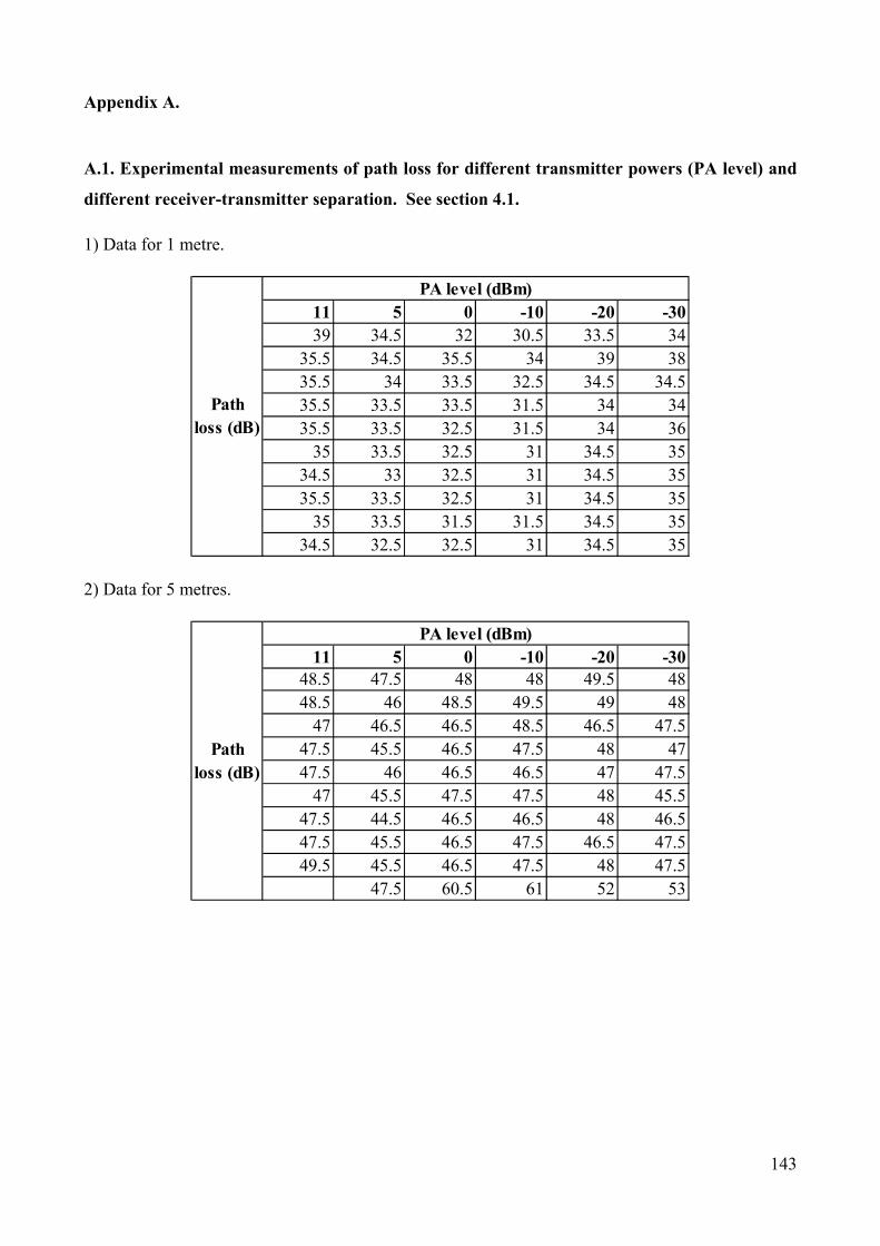
143
Appendix A.
A.1. Experimental measurements of path loss for different transmitter powers (PA level) and
different receiver-transmitter separation. See section 4.1.
1) Data for 1 metre.
2) Data for 5 metres.
11 5 0 -10 -20 -3039 34.5 32 30.5 33.5 34
35.5 34.5 35.5 34 39 3835.5 34 33.5 32.5 34.5 34.535.5 33.5 33.5 31.5 34 3435.5 33.5 32.5 31.5 34 36
35 33.5 32.5 31 34.5 3534.5 33 32.5 31 34.5 3535.5 33.5 32.5 31 34.5 35
35 33.5 31.5 31.5 34.5 3534.5 32.5 32.5 31 34.5 35
PA level (dBm)
Path loss (dB)
11 5 0 -10 -20 -3048.5 47.5 48 48 49.5 4848.5 46 48.5 49.5 49 48
47 46.5 46.5 48.5 46.5 47.547.5 45.5 46.5 47.5 48 4747.5 46 46.5 46.5 47 47.5
47 45.5 47.5 47.5 48 45.547.5 44.5 46.5 46.5 48 46.547.5 45.5 46.5 47.5 46.5 47.549.5 45.5 46.5 47.5 48 47.5
47.5 60.5 61 52 53
PA level (dBm)
Path loss (dB)
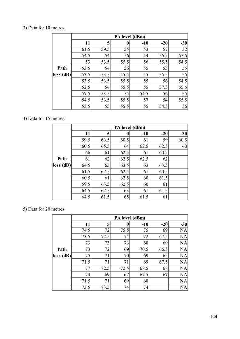
144
3) Data for 10 metres.
4) Data for 15 metres.
5) Data for 20 metres.
11 5 0 -10 -20 -3061.5 59.5 55 53 57 5254.5 54 56 54 56.5 55.5
53 53.5 55.5 56 55.5 54.553.5 54 56 55 55 5553.5 53.5 55.5 55 55.5 5553.5 53.5 55.5 55 56 54.552.5 54 55.5 55 57.5 55.557.5 53.5 55 54.5 56 5554.5 53.5 55.5 57 54 55.553.5 55 55.5 55 54.5 56
PA level (dBm)
Path loss (dB)
11 5 0 -10 -20 -3059.5 63.5 60.5 61 59 60.560.5 65.5 64 62.5 62.5 60
66 61 62.5 61 60.561 62 62.5 62.5 62
64.5 63 63.5 63 63.561.5 62.5 62.5 61 60.560.5 61 62.5 60 61.559.5 63.5 62.5 60 6164.5 62.5 63 61 61.564.5 61.5 65 61.5 61
PA level (dBm)
Path loss (dB)
11 5 0 -10 -20 -3074.5 72 75.5 75 69 NA73.5 72.5 74 72 67.5 NA
73 73 73 68 69 NA73 72 69 70.5 66.5 NA75 71 70 69 65 NA
71.5 71 71 69 67.5 NA77 72.5 72.5 68.5 68 NA74 69 67 67.5 67 NA
71.5 71 69 68 NA73.5 73.5 74 74 NA
PA level (dBm)
Path loss (dB)

145
6) Data for 25 metres.
7) Data for 30 metres.
8) Data for 35 metres.
11 5 0 -10 -20 -3092 78 80.5 74 NA NA79 78.5 80.5 75.5 NA NA81 90 80.5 73 NA NA79 83 80 72.5 NA NA
81.5 78 83 75 NA NA79.5 76.5 75 75.5 NA NA79.5 80 78 72 NA NA82.5 75 78 76 NA NA
73.5 77 NA NANA NA
PA level (dBm)
Path loss (dB)
11 5 0 -10 -20 -3079 79.5 86 70 NA NA83 80.5 83 78.5 NA NA78 78 81 75.5 NA NA92 84 80 78 NA NA81 75.5 79.5 NA NA87 88 88 NA NA
80.5 84.5 79.5 NA NA96.5 86.5 79.5 NA NA
76 82.5 82 NA NA83.5 83.5 86.5 NA NA
PA level (dBm)
Path loss (dB)
11 5 0 -10 -20 -3079 88.5 75.5 75.5 NA NA
79.5 77 75.5 75.5 NA NA90 77.5 77.5 74 NA NA78 77 81 75.5 NA NA
79.5 84.5 85 75 NA NA76 79.5 79.5 73.5 NA NA81 78.5 79 73 NA NA
83.5 79 74 75.5 NA NA88 78 75 78 NA NA84 77.5 79.5 73.5 NA NA
PA level (dBm)
Path loss (dB)

146
9) Data for 40 metres.
10) Data for 45 metres.
11 5 0 -10 -20 -3086.5 88.5 81 77 NA NA90.5 78 78.5 78 NA NA85.5 81 82 78 NA NA87.5 83.5 81 NA NA82.5 85.5 84 NA NA84.5 83.5 85.5 NA NA85.5 84.5 87.5 NA NA88.5 85 84 NA NA83.5 85 86.5 NA NA
86 89 90.5 NA NA
PA level (dBm)
Path loss (dB)
11 5 0 -10 -20 -3096 95 87 79.5 NA NA
94.5 92.5 88 NA NA87 85 82.5 NA NA85 88 84.5 NA NA85 91.5 84 NA NA85 84 88.5 NA NA93 91.5 80.5 NA NA
87.5 92 83.5 NA NA94 84.5 79 NA NA86 89 NA NA
PA level (dBm)
Path loss (dB)

147
Appendix B
B.1. Experiment to determine the path length and number of beacons using the proposed square
grid path. See section 7.5.
1) Node 1 (50, 750,0)
Note : Size is the spacing between anchor.
5 10 20 30
4 8.85 8.19 6.08 5.345 8.13 7.59 7.21 9.016 11.33 7.71 8.80 9.357 8.26 7.70 7.01 8.608 8.08 7.80 7.62 9.779 8.80 9.02 6.89 8.9110 8.36 8.07 5.00 9.5311 8.02 7.55 6.36 NA12 8.03 6.66 5.83 NA13 3.60 6.14 7.45 NA14 4.47 4.39 9.08 NA15 3.58 3.51 6.32 NA16 3.04 4.85 7.00 NA17 2.40 4.44 6.04 NA18 4.01 4.06 7.41 NA19 3.90 5.67 7.94 NA20 3.27 4.04 8.83 NA
Transmitted beacon 40200 10201 2601 1156
Received beacon (max/min)
20/4 20/4 20/4 10/4
Length of path 201km 102km 52km 35km
Size (m)Number of anchor positions
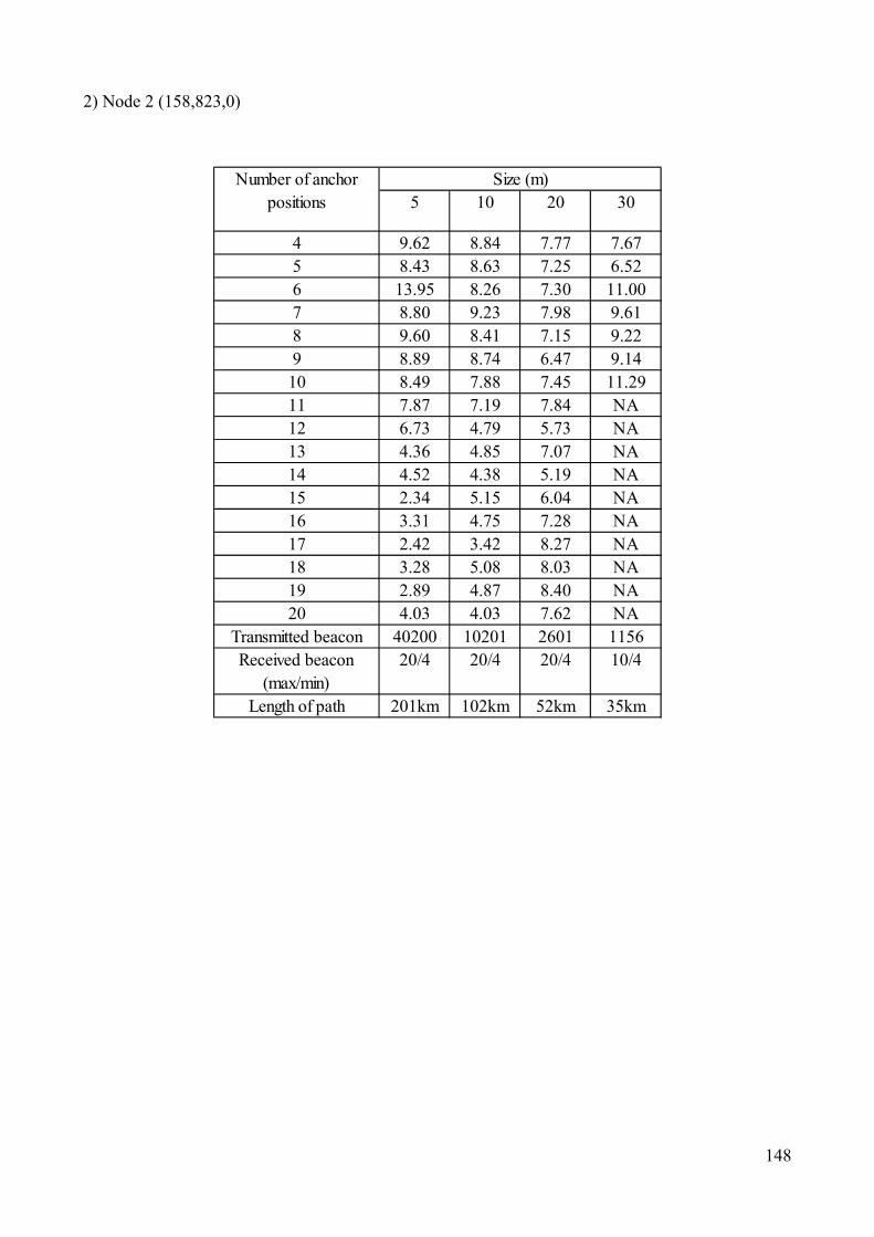
148
2) Node 2 (158,823,0)
5 10 20 30
4 9.62 8.84 7.77 7.675 8.43 8.63 7.25 6.526 13.95 8.26 7.30 11.007 8.80 9.23 7.98 9.618 9.60 8.41 7.15 9.229 8.89 8.74 6.47 9.14
10 8.49 7.88 7.45 11.2911 7.87 7.19 7.84 NA12 6.73 4.79 5.73 NA13 4.36 4.85 7.07 NA14 4.52 4.38 5.19 NA15 2.34 5.15 6.04 NA16 3.31 4.75 7.28 NA17 2.42 3.42 8.27 NA18 3.28 5.08 8.03 NA19 2.89 4.87 8.40 NA20 4.03 4.03 7.62 NA
Transmitted beacon 40200 10201 2601 1156Received beacon
(max/min)20/4 20/4 20/4 10/4
Length of path 201km 102km 52km 35km
Number of anchor positions
Size (m)
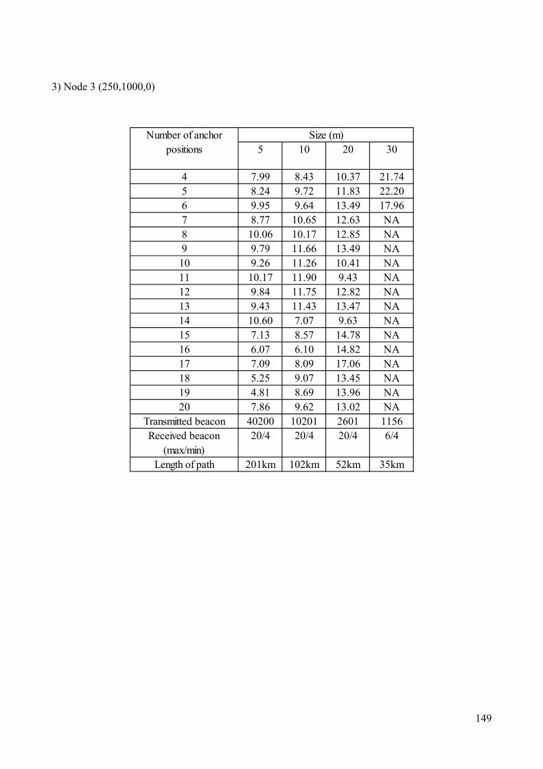
149
3) Node 3 (250,1000,0)
5 10 20 30
4 7.99 8.43 10.37 21.745 8.24 9.72 11.83 22.206 9.95 9.64 13.49 17.967 8.77 10.65 12.63 NA8 10.06 10.17 12.85 NA9 9.79 11.66 13.49 NA
10 9.26 11.26 10.41 NA11 10.17 11.90 9.43 NA12 9.84 11.75 12.82 NA13 9.43 11.43 13.47 NA14 10.60 7.07 9.63 NA15 7.13 8.57 14.78 NA16 6.07 6.10 14.82 NA17 7.09 8.09 17.06 NA18 5.25 9.07 13.45 NA19 4.81 8.69 13.96 NA20 7.86 9.62 13.02 NA
Transmitted beacon 40200 10201 2601 1156Received beacon
(max/min)20/4 20/4 20/4 6/4
Length of path 201km 102km 52km 35km
Number of anchor positions
Size (m)

150
4) Node 4 (380,700,0)
5 10 20 30
4 12.07 24.77 7.87 7.405 9.52 9.73 6.10 9.066 11.54 7.98 7.27 10.057 8.42 8.34 6.67 NA8 7.98 7.94 6.40 NA9 9.18 9.29 8.01 NA10 11.54 8.11 6.85 NA11 12.13 7.30 7.84 NA12 8.12 5.22 6.89 NA13 7.75 4.04 4.47 NA14 2.86 3.84 6.89 NA15 2.13 4.32 7.91 NA16 2.70 4.46 7.84 NA17 3.03 5.05 5.92 NA18 3.05 4.15 9.22 NA19 3.29 4.76 6.89 NA20 2.87 4.73 8.71 NA
Transmitted beacon 40200 10201 2601 1156Received beacon
(max/min)20/4 20/4 20/4 6/4
Length of path 201km 102km 52km 35km
Number of anchor positions
Size (m)

151
5) Node 5 ( 500,500,0)
5 10 20 30
4 8.22 8.23 7.54 7.615 8.85 8.18 7.47 8.986 8.74 8.99 6.42 9.927 8.41 8.43 6.06 7.458 8.47 9.79 6.11 8.889 11.84 8.63 7.75 9.74
10 8.34 8.02 7.45 8.8011 8.02 7.22 8.06 10.1712 7.64 4.86 6.74 10.0013 5.38 3.93 7.64 9.7414 3.81 3.57 5.61 8.6015 3.39 4.07 9.22 NA16 4.04 5.01 7.55 NA17 2.28 4.18 9.72 NA18 3.76 3.92 10.00 NA19 4.63 4.64 8.91 NA20 4.15 4.73 8.14 NA
Transmitted beacon 40200 10201 2601 1156Received beacon
(max/min) 20/4 20/4 20/4 14/4Length of path 201km 102km 52km 35km
Number of anchor positions
Size (m)

152
6) Node 6 (618,800,0)
5 10 20 304 15.01 16.76 7.57 6.085 7.85 15.92 7.38 9.226 7.90 8.82 6.96 10.567 8.22 8.35 6.40 8.308 8.30 8.31 7.07 6.589 7.92 7.78 7.11 10.06
10 13.59 9.15 6.32 8.8311 7.76 7.31 7.21 10.3212 8.51 4.90 8.94 12.9813 3.41 5.42 10.12 10.4114 3.60 4.34 4.74 13.0215 3.67 3.78 7.84 NA16 2.35 3.85 7.16 NA17 3.10 3.87 7.07 NA18 2.67 4.06 7.41 NA19 3.54 4.93 8.51 NA20 3.01 4.17 8.37 NA
Transmitted beacon 40200 10201 2601 1156Received beacon
(max/min)20/4 20/4 20/4 14/4
Length of path 201km 102km 52km 35km
Number of anchor positions
Size (m)

153
7) Node 7 ( 792,795,0)
5 10 20 304 8.85 8.10 10.52 3.915 11.13 7.31 6.81 12.006 7.85 7.59 6.67 11.367 8.00 8.96 7.72 7.718 8.65 7.76 7.99 8.339 8.35 8.62 5.61 5.61
10 8.63 7.98 6.32 8.1511 7.99 7.37 6.36 10.0212 11.82 6.21 6.40 9.3313 5.62 5.20 7.21 13.2314 3.10 5.41 9.74 12.5815 4.23 4.70 9.61 NA16 2.85 4.42 8.24 NA17 3.40 4.46 7.28 NA18 3.68 4.76 7.14 NA19 2.27 4.44 5.74 NA20 2.95 4.86 8.03 NA
Transmitted beacon 40200 10201 2601 1156Received beacon
(max/min)20/4 20/4 20/4 14/4
Length of path 201km 102km 52km 35km
Number of anchor positions
Size (m)

154
8) Node 8 (815,758,0)
5 10 20 304 11.40 62.09 9.14 8.805 11.17 16.24 7.41 9.786 8.31 8.72 6.31 6.057 8.30 7.81 6.15 8.158 8.92 8.28 6.09 9.229 8.08 8.30 8.42 11.5310 13.79 8.06 6.35 13.9111 8.31 8.16 8.06 9.6412 8.31 5.45 6.36 10.0513 3.90 4.41 6.85 10.0514 3.23 4.97 8.50 9.6715 3.76 4.32 8.49 NA16 4.01 5.01 8.77 NA17 2.11 4.64 7.25 NA18 1.60 4.24 8.06 NA19 3.70 3.79 9.14 NA20 2.95 4.79 8.15 NA
Transmitted beacon 40200 10201 2601 1156
Received beacon (max/min)
20/4 20/4 20/4 14/4
Length of path 201km 102km 52km 35km
Number of anchor positions
Size (m)

155
9) Node 9 ( 1000,1000,0)
5 10 20 304 9.63 12.03 18.67 NA5 10.54 22.85 18.55 NA6 10.08 12.81 21.56 NA7 11.50 14.23 14.95 NA8 11.82 14.80 17.75 NA9 12.40 16.72 15.57 NA
10 13.96 17.38 18.73 NA11 13.35 17.74 NA NA12 15.31 19.72 NA NA13 15.21 19.51 NA NA14 17.98 20.44 NA NA15 14.86 13.31 NA NA16 14.36 15.25 NA NA17 11.70 14.88 NA NA18 12.07 14.87 NA NA19 14.08 17.18 NA NA20 13.10 17.15 NA NA
Transmitted beacon 40200 10201 2601 1156
Received beacon (max/min)
20/4 20/4 10/4 NONE
Length of path 201km 102km 52km 35km
Number of anchor positions
Size (m)

156
10) Node 10 (958,46,0)
5 10 20 304 11.70 42.83 9.57 10.975 8.19 8.68 7.09 8.956 7.80 9.79 6.68 10.647 7.70 9.06 7.20 10.058 13.71 8.15 6.47 9.149 8.27 8.25 7.35 8.3710 8.01 7.99 6.96 7.1811 8.16 7.31 5.10 NA12 8.57 4.44 5.74 NA13 3.30 4.75 6.36 NA14 5.98 3.84 5.66 NA15 3.50 4.26 6.00 NA16 2.81 4.64 6.40 NA17 2.95 4.37 8.30 NA18 2.80 3.67 6.85 NA19 2.40 5.36 6.71 NA20 4.13 4.42 6.56 NA
Transmitted beacon 40200 10201 2601 1156
Received beacon (max/min)
20/4 20/4 10/4 10/4
Length of path 201km 102km 52km 35km
Number of anchor positions
Size (m)
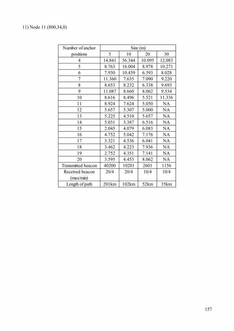
157
11) Node 11 (800,34,0)
5 10 20 304 14.841 56.344 10.095 12.0835 8.763 16.004 8.978 10.2716 7.930 10.459 6.393 8.0287 11.360 7.635 7.090 9.2208 8.653 8.232 6.338 9.6939 11.087 8.660 8.062 9.53410 8.616 8.496 5.521 11.33611 8.924 7.624 5.050 NA12 5.657 5.307 5.000 NA13 5.225 4.510 5.657 NA14 5.031 3.387 6.516 NA15 2.045 4.079 6.083 NA16 4.752 5.042 7.176 NA17 3.321 4.536 6.041 NA18 3.462 4.223 7.936 NA19 2.752 4.351 7.141 NA20 3.595 4.453 8.062 NA
Transmitted beacon 40200 10201 2601 1156Received beacon
(max/min)20/4 20/4 10/4 10/4
Length of path 201km 102km 52km 35km
Number of anchor positions
Size (m)

158
12) Node 12 ( 632, 171, 0)
5 10 20 304 8.77 8.75 6.30 12.405 9.45 9.52 9.14 8.656 10.88 8.05 8.34 7.847 11.15 11.20 8.33 8.068 8.18 8.55 7.44 11.059 8.19 8.20 6.82 7.5510 8.41 8.16 6.00 8.2811 8.21 7.27 6.36 NA12 8.54 5.80 7.28 NA13 4.12 4.96 6.56 NA14 4.67 4.28 6.85 NA15 4.45 4.84 7.55 NA16 2.45 4.82 8.94 NA17 4.36 4.49 8.06 NA18 2.67 5.27 7.71 NA19 3.28 5.52 8.11 NA20 3.67 4.08 7.18 NA
Transmitted beacon 40200 10201 2601 1156
Received beacon (max/min)
20/4 20/4 10/4 10/4
Length of path 201km 102km 52km 35km
Number of anchor positions
Size (m)
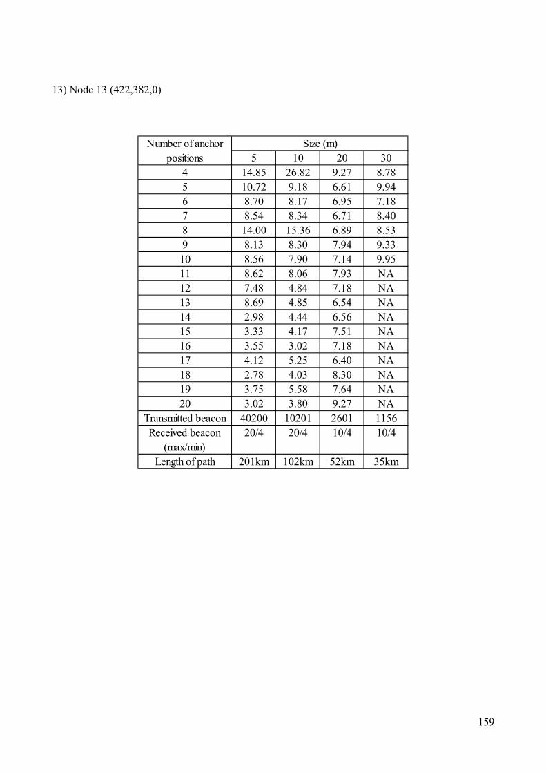
159
13) Node 13 (422,382,0)
5 10 20 304 14.85 26.82 9.27 8.785 10.72 9.18 6.61 9.946 8.70 8.17 6.95 7.187 8.54 8.34 6.71 8.408 14.00 15.36 6.89 8.539 8.13 8.30 7.94 9.33
10 8.56 7.90 7.14 9.9511 8.62 8.06 7.93 NA12 7.48 4.84 7.18 NA13 8.69 4.85 6.54 NA14 2.98 4.44 6.56 NA15 3.33 4.17 7.51 NA16 3.55 3.02 7.18 NA17 4.12 5.25 6.40 NA18 2.78 4.03 8.30 NA19 3.75 5.58 7.64 NA20 3.02 3.80 9.27 NA
Transmitted beacon 40200 10201 2601 1156Received beacon
(max/min)20/4 20/4 10/4 10/4
Length of path 201km 102km 52km 35km
Number of anchor positions
Size (m)

160
14) Node 14 ( 320,500,0)
5 10 20 304 31.62 19.37 7.12 7.235 9.75 11.59 7.72 9.156 8.54 8.35 7.45 11.647 8.46 8.16 6.91 8.038 8.47 8.36 6.42 8.039 8.71 9.56 7.25 5.9210 8.38 8.48 6.71 8.4011 7.93 6.68 8.15 10.1212 7.35 5.91 5.39 10.2513 7.06 3.86 5.55 NA14 4.40 4.50 5.99 NA15 3.43 3.69 6.52 NA16 4.22 4.23 8.97 NA17 4.32 4.14 5.52 NA18 4.06 4.80 9.22 NA19 3.08 5.15 8.60 NA20 3.55 4.81 8.15 NA
Transmitted beacon 40200 10201 2601 1156Received beacon
(max/min)20/4 20/4 20/4 12/4
Length of path 201km 102km 52km 35km
Number of anchor positions
Size (m)
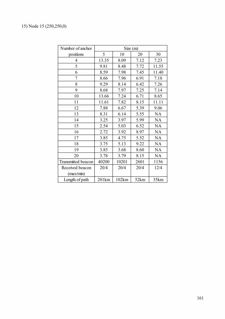
161
15) Node 15 (250,250,0)
5 10 20 304 13.35 8.09 7.12 7.235 9.81 8.48 7.72 11.556 8.59 7.98 7.45 11.407 8.66 7.96 6.91 7.188 9.29 8.14 6.42 7.269 8.68 7.97 7.25 7.14
10 13.66 7.24 6.71 8.6511 11.61 7.82 8.15 11.1112 7.88 6.67 5.39 9.0613 8.31 6.14 5.55 NA14 3.25 3.97 5.99 NA15 2.54 5.03 6.52 NA16 2.72 3.92 8.97 NA17 3.85 4.75 5.52 NA18 3.75 5.13 9.22 NA19 3.83 3.68 8.60 NA20 3.78 3.79 8.15 NA
Transmitted beacon 40200 10201 2601 1156Received beacon
(max/min)20/4 20/4 20/4 12/4
Length of path 201km 102km 52km 35km
Number of anchor positions
Size (m)

162
16) Node 16 (142, 439,0)
5 10 20 30
4 14.39 8.63 7.32 8.225 8.03 8.48 7.54 11.276 8.20 8.37 6.75 9.147 8.72 8.55 6.06 9.678 13.96 8.52 6.88 6.719 8.34 8.57 7.91 10.9810 8.37 8.47 7.07 11.5611 10.16 8.08 7.14 9.4612 8.67 4.57 6.08 11.7013 5.54 6.09 7.41 10.1514 3.82 3.80 5.83 NA15 3.30 4.69 8.64 NA16 3.33 3.68 7.18 NA17 4.02 4.49 7.55 NA18 3.34 4.87 8.15 NA19 2.73 4.79 8.94 NA20 2.85 3.58 8.40 NA
Transmitted beacon 40200 10201 2601 1156Received beacon
(max/min)20/4 20/4 20/4 13/4
Length of path 201km 102km 52km 35km
Number of anchor positions
Size (m)
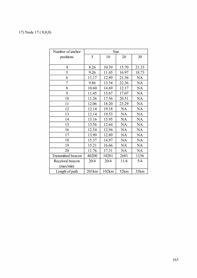
163
17) Node 17 ( 0,0,0)
5 10 20 30
4 8.26 10.39 15.70 21.335 9.26 11.45 16.97 18.736 11.17 12.89 21.36 NA7 9.86 13.54 22.36 NA8 10.60 14.69 12.17 NA9 11.45 15.67 17.07 NA
10 11.26 17.56 20.51 NA11 12.06 18.20 23.29 NA12 12.14 19.18 NA NA13 12.14 19.53 NA NA14 13.16 15.95 NA NA15 13.56 12.64 NA NA16 12.54 12.94 NA NA17 13.99 12.89 NA NA18 15.37 14.97 NA NA19 15.21 16.66 NA NA20 11.76 17.31 NA NA
Transmitted beacon 40200 10201 2601 1156Received beacon
(max/min)20/4 20/4 11/4 5/4
Length of path 201km 102km 52km 35km
Number of anchor positions
Size

164
18) Node 18 (500,1000,0)
5 10 20 304 10.55 9.24 8.27 22.925 10.32 9.88 9.40 21.606 10.05 9.78 12.81 12.267 9.04 9.51 14.37 16.428 11.43 10.58 14.12 NA9 10.69 10.43 12.19 NA10 9.61 10.11 10.02 NA11 9.25 11.57 12.02 NA12 9.56 10.68 11.87 NA13 9.92 11.01 11.22 NA14 10.69 9.51 12.06 NA15 9.76 7.09 15.02 NA16 11.02 8.20 12.10 NA17 6.24 8.81 14.14 NA18 9.22 6.69 12.69 NA19 5.89 7.75 13.53 NA20 6.21 8.06 NA NA
Transmitted beacon 40200 10201 2601 1156Received beacon
(max/min)20/4 20/4 19/4 7/4
Length of path 201km 102km 52km 35km
Number of anchor positions
Size (m)

165
19) Node 19 (700,200,0)
5 10 20 304 15.25 43.69 6.66 7.345 8.27 13.09 5.79 9.386 8.52 8.14 5.67 9.947 8.82 8.43 6.14 8.948 9.67 7.86 6.51 10.829 8.42 9.06 7.89 10.02
10 13.70 8.29 7.85 8.1511 10.77 7.84 6.24 9.8712 3.08 6.65 6.85 NA13 3.10 4.68 7.45 NA14 2.47 5.42 7.14 NA15 3.20 3.88 7.76 NA16 3.74 4.91 7.62 NA17 5.34 4.06 7.18 NA18 4.55 4.15 7.91 NA19 4.00 4.40 8.83 NA20 2.88 5.61 NA NA
Transmitted beacon 40200 10201 2601 1156Received beacon
(max/min)20/4 20/4 19/4 11/4
Length of path 201km 102km 52km 35km
Number of anchor positions
Size (m)
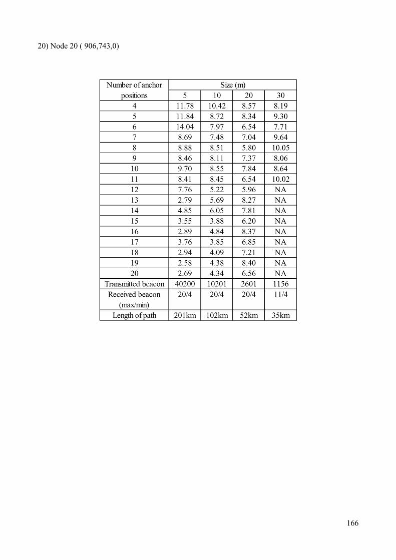
166
20) Node 20 ( 906,743,0)
5 10 20 304 11.78 10.42 8.57 8.195 11.84 8.72 8.34 9.306 14.04 7.97 6.54 7.717 8.69 7.48 7.04 9.648 8.88 8.51 5.80 10.059 8.46 8.11 7.37 8.06
10 9.70 8.55 7.84 8.6411 8.41 8.45 6.54 10.0212 7.76 5.22 5.96 NA13 2.79 5.69 8.27 NA14 4.85 6.05 7.81 NA15 3.55 3.88 6.20 NA16 2.89 4.84 8.37 NA17 3.76 3.85 6.85 NA18 2.94 4.09 7.21 NA19 2.58 4.38 8.40 NA20 2.69 4.34 6.56 NA
Transmitted beacon 40200 10201 2601 1156Received beacon
(max/min)20/4 20/4 20/4 11/4
Length of path 201km 102km 52km 35km
Number of anchor positions
Size (m)

167
21) Node 21 (127,192,0)
5 10 20 304 11.20 8.30 5.75 8.685 7.77 8.80 8.47 12.106 11.53 8.39 7.10 9.147 8.29 8.81 8.58 10.328 7.95 8.68 8.01 10.819 10.98 8.58 6.36 10.0210 8.24 7.52 7.41 8.7711 8.26 8.22 6.04 10.8212 7.82 5.24 5.39 10.1013 7.22 3.81 7.14 8.5414 8.85 4.85 7.26 NA15 3.58 4.27 7.07 NA16 4.25 4.40 8.06 NA17 2.99 4.57 7.14 NA18 2.90 4.00 8.40 NA19 3.63 4.08 9.00 NA20 3.61 4.63 8.03 NA
Transmitted beacon 40200 10201 2601 1156Received beacon
(max/min)20/4 20/4 20/4 13/4
Length of path 201km 102km 52km 35km
Number of anchor positions
Size (m)

168
22) Node 22 (913,655,0)
5 10 20 304 8.23 8.09 9.05 10.235 11.43 8.92 7.84 11.076 8.18 8.79 6.82 9.677 11.58 8.83 7.42 10.508 8.54 8.96 8.67 8.809 8.42 8.07 8.03 9.0810 8.64 8.25 7.07 8.7411 8.06 7.94 5.66 10.9312 8.28 4.94 8.18 11.7413 5.35 4.76 5.24 8.1514 2.99 4.92 6.99 NA15 4.80 4.11 7.25 NA16 3.35 4.49 9.67 NA17 2.91 3.37 7.41 NA18 4.45 4.23 7.28 NA19 2.89 5.32 8.42 NA20 2.83 4.55 8.60 NA
Transmitted beacon 40200 10201 2601 1156Received beacon
(max/min)20/4 20/4 20/4 13/4
Length of path 201km 102km 52km 35km
Number of anchor positions
Size (m)

169
23) Node 23 (98, 706,0)
5 10 20 304 8.30 8.09 9.05 8.155 8.39 8.92 7.84 8.106 9.33 8.79 6.82 11.917 7.95 8.83 7.42 10.418 8.94 8.96 8.67 8.069 8.90 8.07 8.03 8.33
10 11.08 8.25 7.07 9.6511 10.86 7.94 5.66 10.1212 7.01 4.94 8.18 11.2913 6.55 4.76 5.24 NA14 3.64 4.92 6.99 NA15 2.94 4.11 7.25 NA16 3.89 4.49 9.67 NA17 3.28 3.37 7.41 NA18 2.66 4.23 7.28 NA19 3.67 5.32 8.42 NA20 3.03 4.55 8.60 NA
Transmitted beacon 40200 10201 2601 1156Received beacon
(max/min)20/4 20/4 20/4 12/4
Length of path 201km 102km 52km 35km
Number of anchor positions
Size (m)

170
24) Node 24 ( 278,32,0)
5 10 20 304 8.04 14.66 8.87 9.635 10.10 12.78 7.48 9.076 8.37 9.08 7.93 6.747 11.05 8.15 8.83 8.338 8.18 9.41 8.48 7.949 7.90 9.42 7.28 7.4410 13.40 7.84 7.67 9.9511 8.44 7.71 5.39 8.8012 13.34 5.22 7.45 9.7413 5.64 4.53 6.08 NA14 2.33 3.52 7.64 NA15 3.54 5.11 7.14 NA16 4.81 4.32 8.77 NA17 3.49 4.06 6.40 NA18 2.94 3.78 8.77 NA19 2.74 4.23 7.91 NA20 2.65 4.78 7.21 NA
Transmitted beacon 40200 10201 2601 1156Received beacon
(max/min)20/4 20/4 20/4 12/4
Length of path 201km 102km 52km 35km
Number of anchor positions
Size (m)
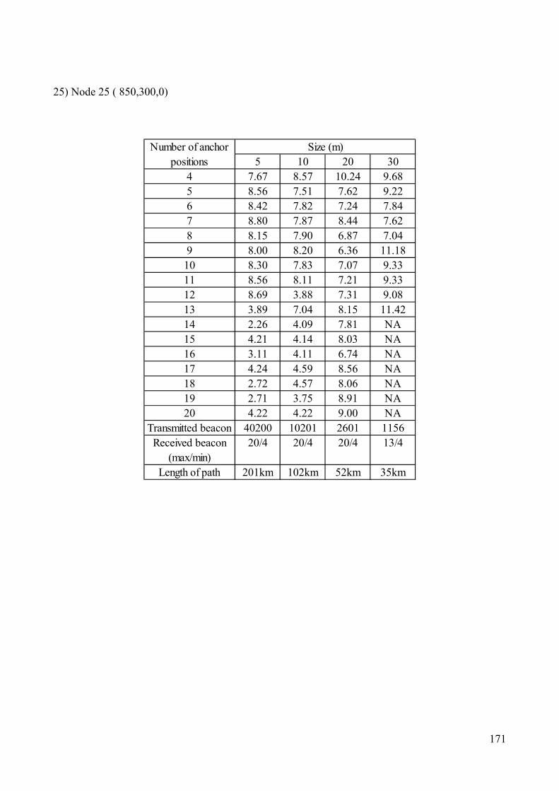
171
25) Node 25 ( 850,300,0)
5 10 20 304 7.67 8.57 10.24 9.685 8.56 7.51 7.62 9.226 8.42 7.82 7.24 7.847 8.80 7.87 8.44 7.628 8.15 7.90 6.87 7.049 8.00 8.20 6.36 11.18
10 8.30 7.83 7.07 9.3311 8.56 8.11 7.21 9.3312 8.69 3.88 7.31 9.0813 3.89 7.04 8.15 11.4214 2.26 4.09 7.81 NA15 4.21 4.14 8.03 NA16 3.11 4.11 6.74 NA17 4.24 4.59 8.56 NA18 2.72 4.57 8.06 NA19 2.71 3.75 8.91 NA20 4.22 4.22 9.00 NA
Transmitted beacon 40200 10201 2601 1156Received beacon
(max/min)20/4 20/4 20/4 13/4
Length of path 201km 102km 52km 35km
Number of anchor positions
Size (m)

172
Appendix C
C.1. Experiment to determine the geometric arrangement of the beacons. See section 7.6.
1) Angle between beacons for 30m spacing.
B1-B2 84 B3-B7 43 B5-B16 B8-B17 B12-B19B1-B3 125 B3-B8 129 B5-B17 B8-B18 B12-B20B1-B4 6 B3-B9 44 B5-B18 B8-B19 B13-B14B1-B5 84 B3-B10 87 B5-B19 B8-B20 B13-B15B1-B6 43 B3-B11 87 B5-B20 B9-B10 129 B13-B16B1-B7 143 B3-B12 70 B6-B7 125 B9-B11 44 B13-B17B1-B8 86 B3-B13 18 B6-B8 44 B9-B12 113 B13-B18B1-B9 86 B3-B14 B6-B9 129 B9-B13 62 B13-B19
B1-B10 125 B3-B15 B6-B10 87 B9-B14 B13-B20B1-B11 43 B3-B16 B6-B11 87 B9-B15 B14-B15B1-B12 141 B3-B17 B6-B12 105 B9-B16 B14-B16B1-B13 141 B3-B18 B6-B13 150 B9-B17 B14-B17B1-B14 B3-B19 B6-B14 B9-B18 B14-B18B1-B15 B3-B20 B6-B15 B9-B19 B14-B19B1-B16 B4-B5 86 B6-B16 B9-B20 B14-B20B1-B17 B4-B6 44 B6-B17 B10-B11 153 B15-B16B1-B18 B4-B7 149 B6-B18 B10-B12 18 B15-B17B1-B19 B4-B8 87 B6-B19 B10-B13 70 B15-B18B1-B20 B4-B9 87 B6-B20 B10-B14 B15-B19B2-B3 43 B4-B10 129 B7-B8 86 B10-B15 B15-B20B2-B4 86 B4-B11 44 B7-B9 86 B10-B16 B16-B17B2-B5 143 B4-B12 145 B7-B10 43 B10-B17 B16-B18B2-B6 125 B4-B13 145 B7-B11 125 B10-B18 B16-B19B2-B7 84 B4-B14 B7-B12 27 B10-B19 B16-B20B2-B8 149 B4-B15 B7-B13 27 B10-B20 B17-B18B2-B9 6 B4-B16 B7-B14 B11-B12 150 B17-B19
B2-B10 125 B4-B17 B7-B15 B11-B13 105 B17-B20B2-B11 43 B4-B18 B7-B16 B11-B14 B18-B19B2-B12 111 B4-B19 B7-B17 B11-B15 B18-B20B2-B13 62 B4-B20 B7-B18 B11-B16 B19-B20B2-B14 B5-B6 43 B7-B19 B11-B17B2-B15 B5-B7 84 B7-B20 B11-B18B2-B16 B5-B8 6 B8-B9 156 B11-B19B2-B17 B5-B9 149 B8-B10 44 B11-B20B2-B18 B5-B10 43 B8-B11 129 B12-B13 52B2-B19 B5-B11 125 B8-B12 62 B12-B14B2-B20 B5-B12 62 B8-B13 113 B12-B15B3-B4 129 B5-B13 111 B8-B14 B12-B16B3-B5 125 B5-B14 B8-B15 B12-B17B3-B6 153 B5-B15 B8-B16 B12-B18
Size (m) 30Localization error (m) 5.42
Angle between each beacons:

173
2) Angle between beacons for 40m spacing.
B1-B2 87 B3-B7 27 B5-B16 B8-B17 B12-B19B1-B3 87 B3-B8 B5-B17 B8-B18 B12-B20B1-B4 152 B3-B9 B5-B18 B8-B19 B13-B14B1-B5 44 B3-B10 B5-B19 B8-B20 B13-B15B1-B6 44 B3-B11 B5-B20 B9-B10 B13-B16B1-B7 62 B3-B12 B6-B7 106 B9-B11 B13-B17B1-B8 B3-B13 B6-B8 B9-B12 B13-B18B1-B9 B3-B14 B6-B9 B9-B13 B13-B19B1-B10 B3-B15 B6-B10 B9-B14 B13-B20B1-B11 B3-B16 B6-B11 B9-B15 B14-B15B1-B12 B3-B17 B6-B12 B9-B16 B14-B16B1-B13 B3-B18 B6-B13 B9-B17 B14-B17B1-B14 B3-B19 B6-B14 B9-B18 B14-B18B1-B15 B3-B20 B6-B15 B9-B19 B14-B19B1-B16 B4-B5 129 B6-B16 B9-B20 B14-B20B1-B17 B4-B6 129 B6-B17 B10-B11 B15-B16B1-B18 B4-B7 113 B6-B18 B10-B12 B15-B17B1-B19 B4-B8 B6-B19 B10-B13 B15-B18B1-B20 B4-B9 B6-B20 B10-B14 B15-B19B2-B3 152 B4-B10 B7-B8 B10-B15 B15-B20B2-B4 87 B4-B11 B7-B9 B10-B16 B16-B17B2-B5 129 B4-B12 B7-B10 B10-B17 B16-B18B2-B6 44 B4-B13 B7-B11 B10-B18 B16-B19B2-B7 145 B4-B14 B7-B12 B10-B19 B16-B20B2-B8 B4-B15 B7-B13 B10-B20 B17-B18B2-B9 B4-B16 B7-B14 B11-B12 B17-B19B2-B10 B4-B17 B7-B15 B11-B13 B17-B20B2-B11 B4-B18 B7-B16 B11-B14 B18-B19B2-B12 B4-B19 B7-B17 B11-B15 B18-B20B2-B13 B4-B20 B7-B18 B11-B16 B19-B20B2-B14 B5-B6 88 B7-B19 B11-B17B2-B15 B5-B7 18 B7-B20 B11-B18B2-B16 B5-B8 B8-B9 B11-B19B2-B17 B5-B9 B8-B10 B11-B20B2-B18 B5-B10 B8-B11 B12-B13B2-B19 B5-B11 B8-B12 B12-B14B2-B20 B5-B12 B8-B13 B12-B15B3-B4 87 B5-B13 B8-B14 B12-B16B3-B5 44 B5-B14 B8-B15 B12-B17B3-B6 129 B5-B15 B8-B16 B12-B18
Size (m) 40Localization error (m) 7.29
Angle between each beacons:
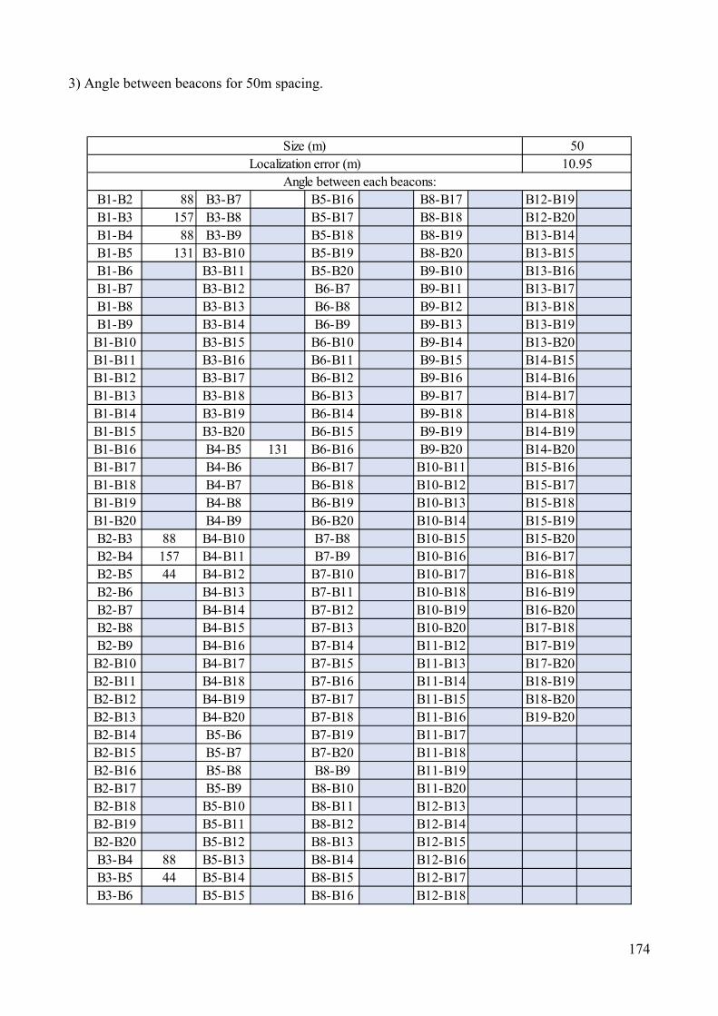
174
3) Angle between beacons for 50m spacing.
B1-B2 88 B3-B7 B5-B16 B8-B17 B12-B19B1-B3 157 B3-B8 B5-B17 B8-B18 B12-B20B1-B4 88 B3-B9 B5-B18 B8-B19 B13-B14B1-B5 131 B3-B10 B5-B19 B8-B20 B13-B15B1-B6 B3-B11 B5-B20 B9-B10 B13-B16B1-B7 B3-B12 B6-B7 B9-B11 B13-B17B1-B8 B3-B13 B6-B8 B9-B12 B13-B18B1-B9 B3-B14 B6-B9 B9-B13 B13-B19
B1-B10 B3-B15 B6-B10 B9-B14 B13-B20B1-B11 B3-B16 B6-B11 B9-B15 B14-B15B1-B12 B3-B17 B6-B12 B9-B16 B14-B16B1-B13 B3-B18 B6-B13 B9-B17 B14-B17B1-B14 B3-B19 B6-B14 B9-B18 B14-B18B1-B15 B3-B20 B6-B15 B9-B19 B14-B19B1-B16 B4-B5 131 B6-B16 B9-B20 B14-B20B1-B17 B4-B6 B6-B17 B10-B11 B15-B16B1-B18 B4-B7 B6-B18 B10-B12 B15-B17B1-B19 B4-B8 B6-B19 B10-B13 B15-B18B1-B20 B4-B9 B6-B20 B10-B14 B15-B19B2-B3 88 B4-B10 B7-B8 B10-B15 B15-B20B2-B4 157 B4-B11 B7-B9 B10-B16 B16-B17B2-B5 44 B4-B12 B7-B10 B10-B17 B16-B18B2-B6 B4-B13 B7-B11 B10-B18 B16-B19B2-B7 B4-B14 B7-B12 B10-B19 B16-B20B2-B8 B4-B15 B7-B13 B10-B20 B17-B18B2-B9 B4-B16 B7-B14 B11-B12 B17-B19
B2-B10 B4-B17 B7-B15 B11-B13 B17-B20B2-B11 B4-B18 B7-B16 B11-B14 B18-B19B2-B12 B4-B19 B7-B17 B11-B15 B18-B20B2-B13 B4-B20 B7-B18 B11-B16 B19-B20B2-B14 B5-B6 B7-B19 B11-B17B2-B15 B5-B7 B7-B20 B11-B18B2-B16 B5-B8 B8-B9 B11-B19B2-B17 B5-B9 B8-B10 B11-B20B2-B18 B5-B10 B8-B11 B12-B13B2-B19 B5-B11 B8-B12 B12-B14B2-B20 B5-B12 B8-B13 B12-B15B3-B4 88 B5-B13 B8-B14 B12-B16B3-B5 44 B5-B14 B8-B15 B12-B17B3-B6 B5-B15 B8-B16 B12-B18
Size (m) 50Localization error (m) 10.95
Angle between each beacons:

175
4) Angle between beacons for 60m spacing.
B1-B2 88 B3-B7 B5-B16 B8-B17 B12-B19B1-B3 45 B3-B8 B5-B17 B8-B18 B12-B20B1-B4 B3-B9 B5-B18 B8-B19 B13-B14B1-B5 B3-B10 B5-B19 B8-B20 B13-B15B1-B6 B3-B11 B5-B20 B9-B10 B13-B16B1-B7 B3-B12 B6-B7 B9-B11 B13-B17B1-B8 B3-B13 B6-B8 B9-B12 B13-B18B1-B9 B3-B14 B6-B9 B9-B13 B13-B19
B1-B10 B3-B15 B6-B10 B9-B14 B13-B20B1-B11 B3-B16 B6-B11 B9-B15 B14-B15B1-B12 B3-B17 B6-B12 B9-B16 B14-B16B1-B13 B3-B18 B6-B13 B9-B17 B14-B17B1-B14 B3-B19 B6-B14 B9-B18 B14-B18B1-B15 B3-B20 B6-B15 B9-B19 B14-B19B1-B16 B4-B5 B6-B16 B9-B20 B14-B20B1-B17 B4-B6 B6-B17 B10-B11 B15-B16B1-B18 B4-B7 B6-B18 B10-B12 B15-B17B1-B19 B4-B8 B6-B19 B10-B13 B15-B18B1-B20 B4-B9 B6-B20 B10-B14 B15-B19B2-B3 132 B4-B10 B7-B8 B10-B15 B15-B20B2-B4 B4-B11 B7-B9 B10-B16 B16-B17B2-B5 B4-B12 B7-B10 B10-B17 B16-B18B2-B6 B4-B13 B7-B11 B10-B18 B16-B19B2-B7 B4-B14 B7-B12 B10-B19 B16-B20B2-B8 B4-B15 B7-B13 B10-B20 B17-B18B2-B9 B4-B16 B7-B14 B11-B12 B17-B19
B2-B10 B4-B17 B7-B15 B11-B13 B17-B20B2-B11 B4-B18 B7-B16 B11-B14 B18-B19B2-B12 B4-B19 B7-B17 B11-B15 B18-B20B2-B13 B4-B20 B7-B18 B11-B16 B19-B20B2-B14 B5-B6 B7-B19 B11-B17B2-B15 B5-B7 B7-B20 B11-B18B2-B16 B5-B8 B8-B9 B11-B19B2-B17 B5-B9 B8-B10 B11-B20B2-B18 B5-B10 B8-B11 B12-B13B2-B19 B5-B11 B8-B12 B12-B14B2-B20 B5-B12 B8-B13 B12-B15B3-B4 B5-B13 B8-B14 B12-B16B3-B5 B5-B14 B8-B15 B12-B17B3-B6 B5-B15 B8-B16 B12-B18
Size (m) 60Localization error (m) 15.14
Angle between each beacons:

176
Appendix D
D.1. Experiment to determine the localization error for each blind node by varying the node
density of 50, 100 and 200 nodes. See section 8.2.2.
1) Localization error for 50 blind nodes.
6G3
x y z x y z x y z PL Est d (m)
1 319 228 0 19.16 300 250 10 76 26350 200 13 82 39350 250 13 82 39300 200 10 83 42250 250 13 86 51290 273 0 86 51
2 232 12 0 18.03 250 0 13 71 18218 37 0 75 24250 50 13 79 32200 50 10 82 39200 0 10 87 55300 0 10 88 59
3 481 439 0 11.31 476 445 04 251 92 0 14.04 250 100 13 73 21
230 108 0 76 26300 50 10 82 39250 50 13 83 42200 100 10 87 55300 100 10 87 55
5 96 19 0 11.40 96 43 0 72 20100 0 10 75 24100 50 10 76 2650 50 13 83 4250 0 13 85 48
150 50 13 87 55
6 420 240 0 15.17 432 222 07 222 253 0 13.93 224 252 08 281 275 0 16.34 290 273 0 59 8
250 250 13 79 32300 250 10 80 34300 300 10 80 34224 252 0 84 45250 300 13 87 55
9 87 340 0 13.38 86 353 010 390 43 0 14.87 392 44 011 207 424 0 16.37 201 417 012 114 111 0 11.40 112 103 013 22 481 014 385 111 0 19.05 381 103 0
Number of anchor positions66
UN
Number Blind node positions
Local anchor from G1 Mobile anchor + Local anchorG1 G2
Error Error

177
15 247 140 0 7.62 250 150 13 74 23250 172 0 79 32230 108 0 80 34250 100 13 84 45250 200 13 84 45300 100 10 85 48
16 165 101 0 14.71 150 101 017 442 9 018 235 91 0 16.48 230 108 019 130 296 0 12.41 125 312 020 231 198 0 8.06 250 150 13 69 16
250 172 0 80 34300 150 10 83 42250 100 13 84 45200 150 10 85 48250 200 13 85 48
21 37 46 022 208 284 0 16.18 199 282 023 265 179 0 16.42 250 172 024 362 388 0 13.75 333 378 025 26 269 0 17.68 50 250 13 78 30
0 250 10 83 4250 300 13 84 45
0 300 10 85 480 200 10 87 55
100 250 10 89 63
26 384 302 0 10.91 400 300 10 78 30350 300 13 84 45400 250 10 86 51400 350 10 88 59389 258 0 88 59361 388 0 88 59
27 363 377 0 13.87 364 367 028 448 342 0 9.33 455 348 029 356 427 0 16.48 352 408 030 321 437 0 16.40 319 443 031 384 264 0 11.85 389 258 032 349 394 0 10.53 361 388 033 102 321 0 12.65 107 326 034 80 33 0 15.81 96 43 035 393 84 0 15.30 399 91 036 169 397 0 15.00 154 402 037 299 20 0 17.00 305 47 038 336 99 0 13.66 341 94 039 215 32 0 12.04 218 37 040 291 385 0 12.12 290 390 041 166 64 0 11.87 150 50 13 75 24
150 100 13 78 30200 100 10 85 48150 101 0 87 55230 108 0 89 63100 50 10 90 68

178
2) Localization error for 100 blind nodes.
42 166 488 0 18.74 161 473 043 244 330 0 13.69 241 341 044 315 287 0 12.23 290 273 045 399 278 0 9.61 389 258 0 70 17
350 300 13 77 28400 300 10 81 37400 250 10 84 45350 250 13 85 48450 250 13 86 51
46 223 289 0 10.61 200 300 10 72 20199 282 0 76 26200 250 10 81 37250 300 13 81 37224 252 0 83 42250 250 13 86 51
47 454 206 0 8.56 455 224 048 482 334 0 20.11 481 346 049 463 449 0 8.42 464 452 050 454 172 0 14.68 449 153 0
6G3
x y z x y z x y z PL Est d (m)
1 319 228 0 14.6625 305 238 02 232 12 0 12.2858 250 0 13 73 21
210 35 0 79 32200 0 10 81 37250 50 13 84 45297 13 0 84 45300 50 10 87 55
3 481 439 0 10.8103 473 438 0 64 11500 450 10 71 18463 445 0 71 18450 450 13 76 26500 400 10 79 32471 383 0 84 45
4 251 92 0 12.0208 250 91 05 96 19 0 16.4438 98 35 06 420 240 0 13.9284 425 264 07 222 253 0 9.47214 200 250 10 74 23
219 284 0 80 34193 284 0 81 37250 250 13 82 39250 200 13 84 45246 203 0 85 48
8 281 275 0 7.03553 296 308 0 75 24300 300 10 78 30310 258 0 79 32300 250 10 83 42305 238 0 85 48300 200 10 86 51
9 87 340 0 14.2086 82 358 010 390 43 0 14.8661 384 40 011 207 424 0 15.9834 182 413 012 114 111 0 10.4842 61 105 013 22 481 0
Mobile anchor + Local anchor UN
Number Blind node positions Number of anchor positions6 6
G1 G2Error Local anchor from G1 Error

179
14 385 111 0 10.877 381 123 0 73 21370 89 0 73 21367 99 0 73 21400 100 10 76 26401 89 0 78 30400 150 10 84 45
15 247 140 0 12.6916 238 128 016 165 101 0 14 170 108 017 442 9 0 13.4654 450 0 13 68 15
450 50 13 84 45384 40 0 86 51400 0 10 87 55500 50 10 87 55500 0 10 89 63
18 235 91 0 12.4496 245 99 019 130 296 0 13.9104 129 301 020 231 198 0 14.2652 246 203 021 37 46 0 7.83902 48 58 022 208 284 0 13.1708 219 284 0 62 10
200 300 10 69 16193 284 0 70 17200 250 10 79 32250 250 13 81 37150 300 13 82 39
23 265 179 0 16.1063 250 183 024 362 388 0 15.6944 338 387 025 26 269 0 18.6011 36 281 026 384 302 0 10.3852 392 305 027 363 377 0 17.2761 359 400 028 448 342 0 10.0499 456 306 029 356 427 0 12.037 350 450 13 76 26
367 406 0 76 26400 450 10 80 34359 400 0 80 34308 416 0 82 39338 387 0 85 48
30 321 437 0 11.2236 308 416 0 72 20300 450 10 77 28350 450 13 78 30350 400 13 83 42300 400 10 84 45250 450 13 85 48
31 384 264 0 18.5603 402 259 032 349 394 0 10.7935 367 406 033 102 321 0 14.933 73 344 034 80 33 0 8.57316 98 35 0 73 21
100 50 10 75 2450 50 13 79 3248 58 0 80 3450 0 13 82 3987 66 0 82 39
35 393 84 0 10.1699 401 89 036 169 397 0 17.3747 178 420 037 299 20 0 11.8523 297 13 038 336 99 0 11.4878 338 106 039 215 32 0 13.5903 210 35 040 291 385 0 14.9994 277 390 041 166 64 0 19.2082 157 62 042 166 488 043 244 330 0 16.1555 244 344 044 315 287 0 15.0664 310 258 045 399 278 0 12.54 388 289 046 223 289 0 12.8929 219 284 047 454 206 0 10 447 203 0

180
48 482 334 0 21.0109 472 336 049 463 449 0 11.8517 463 445 050 454 172 0 13.0384 459 194 051 342 494 0 11.0765 346 487 052 66 85 0 14.6441 53 97 053 361 129 0 15.5242 381 123 054 55 198 0 10.6217 51 195 055 59 37 0 10.7002 98 35 0 72 20
50 50 13 73 21100 50 10 80 34100 0 10 84 45
87 66 0 84 4548 58 0 85 48
56 320 342 0 15.582 336 341 057 164 201 0 9.46041 159 202 058 327 491 0 14.4222 346 487 0 69 16
300 500 10 76 26350 500 13 79 32300 450 10 80 34350 450 13 86 51400 500 10 87 55
59 375 201 0 18.841 340 205 060 292 310 0 11.4211 296 308 061 370 77 0 17.0294 370 89 062 117 191 0 13.4716 116 175 063 367 81 0 19.4043 367 99 064 485 379 0 20.1246 471 383 065 433 436 0 20.6782 432 443 066 43 175 0 15.2971 40 158 067 183 343 0 13.2082 152 349 068 185 147 0 13.3199 189 156 069 343 265 0 10.3192 342 288 070 299 416 0 14.9768 308 416 071 395 299 0 11 392 305 0 58 8
400 300 10 62 10388 289 0 68 15425 264 0 80 34402 259 0 81 37400 350 10 82 39
72 184 168 0 8.15423 189 156 0 69 16200 150 10 80 34157 181 0 80 34150 200 13 82 39200 200 10 85 48250 183 0 85 48
73 103 150 0 9.22559 96 145 074 43 226 0 14.3824 51 237 075 386 211 0 14.3178 388 197 076 103 180 0 17.3344 132 182 077 194 279 0 11.6317 193 284 078 276 371 0 15.0488 280 388 079 114 212 0 14.2127 110 206 080 321 215 0 12.1241 323 206 081 242 62 0 11.4878 241 52 0 65 12
250 50 13 73 21210 35 0 77 28245 99 0 79 32250 91 0 82 39250 100 13 84 45

181
82 76 12 0 10.9788 98 35 0 76 2650 0 13 77 28
100 0 10 80 34100 50 10 86 51
50 50 13 86 5187 66 0 87 55
83 391 145 0 12.2009 400 150 10 61 9381 123 0 76 26400 100 10 82 39350 100 13 85 48350 150 13 85 48388 197 0 85 48
84 50 159 0 11.1803 47 184 085 147 327 0 15.0166 146 334 086 119 478 0 10.8167 100 450 10 76 26
100 500 10 80 34150 450 13 81 37150 500 13 85 48
50 450 13 86 51200 500 10 88 59
87 265 468 0 14.5602 271 441 088 46 229 0 15.1488 37 207 089 203 120 0 17.8018 200 103 090 52 382 0 14.7159 63 397 091 56 380 0 15.2807 51 396 092 177 358 0 14.1774 192 352 093 486 428 0 18.7883 473 438 094 173 141 0 450 364 0 13.3772 189 156 0 69 16
150 150 13 76 26170 108 0 77 28200 100 10 80 34200 150 10 81 37150 100 13 81 37
95 443 366 0 14.3972 450 364 096 227 69 0 19.6177 241 52 097 207 418 0 14.2268 212 411 098 109 69 0 13.0384 87 66 099 63 294 0 13.3007 50 300 13 72 20
36 281 0 79 3250 250 13 80 3473 344 0 82 39
100 300 10 86 51100 350 10 86 51
100 154 183 0 9.74342 157 181 0

182
3) Localization error for 200 blind nodes.
x y z x y z x y z PL Est d (m)
1 319 228 0 9.22 316 216 0 62 14350 200 13 77 28300 250 10 81 37350 250 13 83 42300 200 10 84 45275 261 0 84 45
2 232 12 0 15.30 250 0 13 73 21250 50 13 77 28216 36 0 79 32200 50 10 82 38200 0 10 83 42175 69 0 86 51
3 481 439 0 14.18 500 450 10 70 17445 428 0 83 42450 450 13 84 45432 439 0 84 45450 400 13 88 59500 400 10 89 63
4 251 92 0 15.04 242 92 05 96 19 0 16.55 98 36 06 420 240 0 10.25 418 224 07 222 253 0 16.84 208 256 08 281 275 0 18.03 282 277 09 87 340 0 15.23 91 341 0
10 390 43 0 10.10 373 60 011 207 424 0 13.91 194 429 012 114 111 0 12.42 113 119 013 22 481 0 14.35 0 500 10 77 28
50 450 13 79 3250 500 13 83 42
0 450 10 88 5953 419 0 88 5992 458 0 90 68
14 385 111 0 10.56 388 109 0 52 10400 100 10 72 22373 130 0 74 23350 150 13 81 37362 68 0 81 37400 150 10 82 38
15 247 140 0 11.18 264 130 016 165 101 0 10.34 150 100 13 70 17
175 74 0 72 20146 104 0 75 24179 87 0 75 24175 69 0 78 30188 116 0 80 34
17 442 9 0 10.24 450 0 13 67 16436 59 0 81 37450 50 0 81 37400 0 10 84 45386 23 0 84 45500 0 10 85 48
G2
Mobile anchor + Local anchor
Number of anchor positions6
Error
6
Error Local anchor from G1
G1
Number Blind node positions
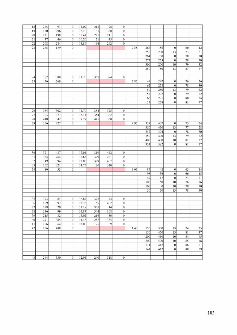
183
18 235 91 0 14.09 212 98 019 130 296 0 12.10 135 320 020 231 198 0 15.41 221 211 021 37 46 0 10.20 21 45 022 208 284 0 15.89 194 292 023 265 179 0 7.55 263 186 0 60 12
250 200 13 73 21264 130 0 78 30273 223 0 78 30300 200 10 79 32250 150 13 81 37
24 362 388 0 11.70 357 394 025 26 269 0 7.85 49 247 0 76 26
62 228 0 78 3050 250 13 79 3253 297 0 79 3266 271 0 80 3433 228 0 81 37
26 384 302 0 11.70 384 325 027 363 377 0 15.11 354 382 028 448 342 0 9.77 445 350 029 356 427 0 9.95 329 407 0 75 24
350 450 13 77 28357 394 0 78 30350 400 13 79 32400 400 10 81 37354 382 0 81 37
30 321 437 0 17.01 319 442 031 384 264 0 12.65 399 261 032 349 394 0 12.06 329 407 033 102 321 0 14.75 120 320 034 80 33 0 9.03 87 42 0 63 14
98 36 0 66 1549 17 0 73 21
100 50 10 76 26100 0 10 78 30
50 50 13 78 30
35 393 84 0 16.87 376 74 036 169 397 0 12.75 155 402 037 299 20 0 11.18 305 14 038 336 99 0 14.87 344 108 039 215 32 0 13.02 216 36 040 291 385 0 14.18 287 385 041 166 64 0 13.00 175 69 042 166 488 0 11.40 150 500 13 74 23
150 450 13 81 37200 450 10 84 45200 500 10 85 48114 447 0 86 51141 417 0 88 59
43 244 330 0 12.04 240 318 0

184
44 315 287 0 9.06 316 281 0 55 11339 281 0 71 19300 300 10 74 23345 303 0 77 28282 277 0 81 37350 300 13 82 38
45 399 278 0 13.87 392 285 046 223 289 0 14.21 225 279 047 454 206 0 7.00 449 205 048 482 334 0 19.22 455 374 049 463 449 0 11.63 450 450 13 73
445 428 0 75500 450 10 81450 400 13 83432 439 0 83450 500 13 85
50 454 172 0 13.47 454 156 051 342 494 0 11.87 334 491 0 61
343 474 0 71350 500 13 74300 450 10 81400 500 10 82319 442 0 83
52 66 85 0 16.55 82 73 053 361 129 0 14.64 373 130 054 55 198 0 8.33 62 228 055 59 37 0 14.68 49 17 056 320 342 0 15.00 317 329 057 164 201 0 17.46 151 188 0 71
150 200 13 74191 190 0 76200 200 10 81128 153 0 82200 196 0 83
58 327 491 0 13.42 334 491 059 375 201 0 10.02 350 200 13 74
400 200 10 76350 250 13 84418 224 0 84316 216 0 84350 150 13 87
60 292 310 0 12.67 288 332 061 370 77 0 13.00 362 68 062 117 191 0 10.55 108 190 063 367 81 0 12.37 348 83 064 485 379 0 20.52 498 374 065 433 436 0 12.08 432 439 066 43 175 0 9.92 37 162 0 71
50 150 13 7450 200 13 7798 186 0 8196 180 0 8339 215 0 83

185
67 183 343 0 15.86 174 325 068 185 147 0 13.25 179 136 0 63
176 153 0 63200 150 10 71191 190 0 72188 116 0 76222 139 0 77
69 343 265 0 11.44 339 281 0 70350 250 13 72392 285 0 80345 303 0 81381 285 0 84350 300 13 85
70 299 416 0 15.26 309 446 071 395 299 0 7.28 381 285 072 184 168 0 13.60 191 190 073 103 150 0 12.04 102 152 074 43 226 0 12.90 33 228 075 386 211 0 10.80 400 200 10 73
418 224 0 80373 252 0 82391 155 0 84423 240 0 84350 200 13 85
76 103 180 0 12.50 96 180 077 194 279 0 13.68 200 275 078 276 371 0 12.78 287 385 0 64
287 367 0 69309 368 0 75250 350 13 78300 350 10 79250 400 13 81
79 114 212 0 19.74 121 226 080 321 215 0 14.56 316 216 081 242 62 0 14.27 255 74 082 76 12 0 12.18 49 17 0 76
100 0 10 7750 0 13 7887 42 0 8198 36 0 83
125 31 0 83
83 391 145 0 11.40 391 155 084 50 159 0 13.64 37 162 085 147 327 0 4.80 150 340 0 62
135 320 0 68174 325 0 72150 300 13 78150 350 13 78120 320 0 78
86 119 478 0 9.24 114 447 0 75150 450 13 80
92 458 0 81100 500 10 82150 500 13 82141 417 0 83
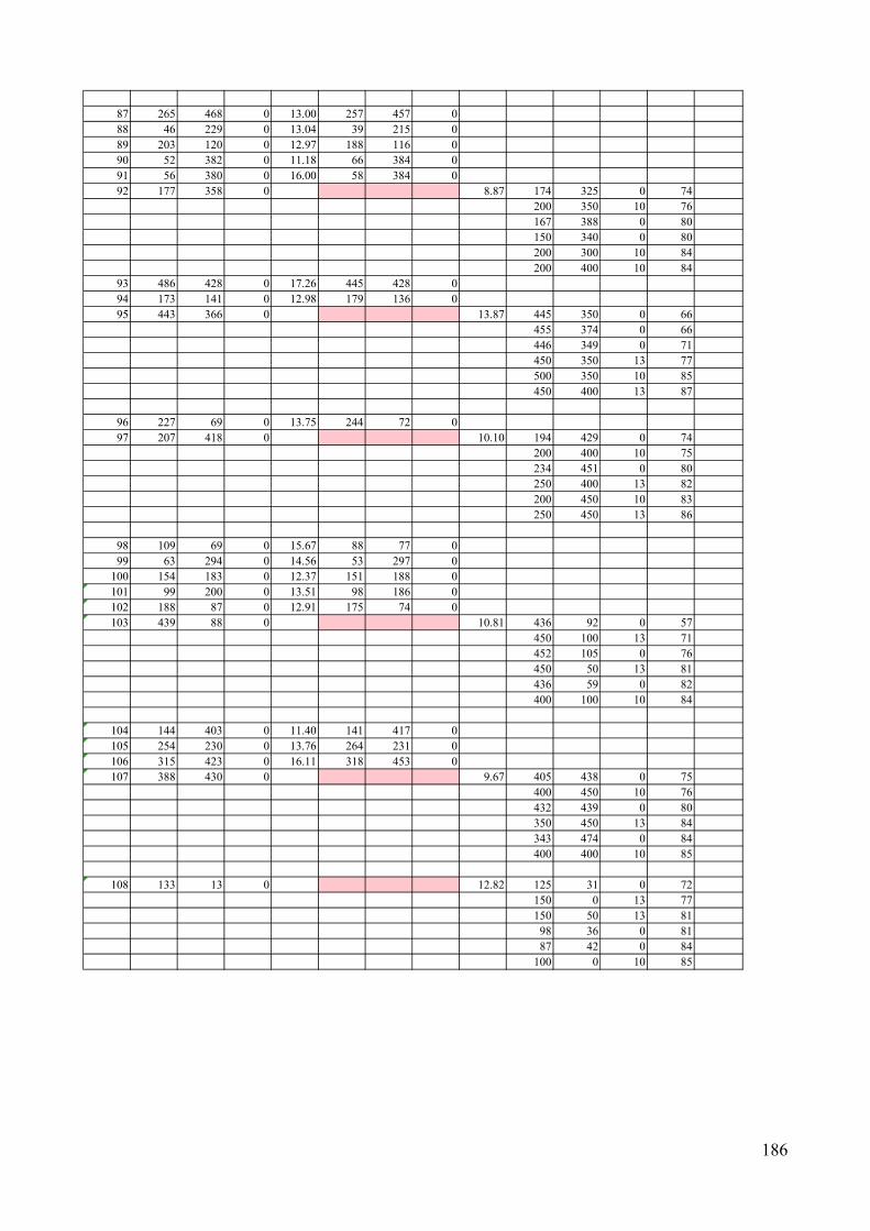
186
87 265 468 0 13.00 257 457 088 46 229 0 13.04 39 215 089 203 120 0 12.97 188 116 090 52 382 0 11.18 66 384 091 56 380 0 16.00 58 384 092 177 358 0 8.87 174 325 0 74
200 350 10 76167 388 0 80150 340 0 80200 300 10 84200 400 10 84
93 486 428 0 17.26 445 428 094 173 141 0 12.98 179 136 095 443 366 0 13.87 445 350 0 66
455 374 0 66446 349 0 71450 350 13 77500 350 10 85450 400 13 87
96 227 69 0 13.75 244 72 097 207 418 0 10.10 194 429 0 74
200 400 10 75234 451 0 80250 400 13 82200 450 10 83250 450 13 86
98 109 69 0 15.67 88 77 099 63 294 0 14.56 53 297 0
100 154 183 0 12.37 151 188 0101 99 200 0 13.51 98 186 0102 188 87 0 12.91 175 74 0103 439 88 0 10.81 436 92 0 57
450 100 13 71452 105 0 76450 50 13 81436 59 0 82400 100 10 84
104 144 403 0 11.40 141 417 0105 254 230 0 13.76 264 231 0106 315 423 0 16.11 318 453 0107 388 430 0 9.67 405 438 0 75
400 450 10 76432 439 0 80350 450 13 84343 474 0 84400 400 10 85
108 133 13 0 12.82 125 31 0 72150 0 13 77150 50 13 81
98 36 0 8187 42 0 84
100 0 10 85

187
109 124 166 0 16.40 128 153 0110 248 409 0 13.46 258 422 0111 48 425 0 10.51 53 419 0112 59 371 0 12.12 34 377 0113 285 260 0 13.42 275 261 0114 206 142 0 12.21 222 139 0115 454 166 0 12.19 469 176 0116 1 286 0 13.51 0 300 10 72
0 250 10 7650 300 13 8650 250 13 8739 215 0 88
0 350 10 89
117 192 492 0 17.22 200 500 10 69150 500 13 84200 450 10 85250 500 13 86257 457 0 90258 422 0 90
118 103 153 0 9.90 114 162 0119 17 75 0 19.79 32 59 0120 245 203 0 10.13 250 200 13 68
221 211 0 73273 223 0 76264 231 0 78200 200 10 79263 186 0 79
121 466 388 0 9.33 455 374 0 73498 374 0 77446 349 0 77450 400 13 79500 400 10 80445 350 0 80
122 106 292 0 12.27 66 301 0123 48 267 0 11.66 49 247 0124 253 340 0 15.30 287 367 0125 190 56 0 13.63 200 50 10 65
175 69 0 73179 87 0 75175 74 0 76250 50 13 81216 36 0 81
126 249 130 0 13.91 244 114 0127 111 418 0 11.69 100 400 10 67
103 408 0 68114 447 0 78150 400 13 80
96 450 0 80141 417 0 81
128 461 370 0 9.20 455 374 0 54446 349 0 74500 350 10 75445 350 0 75450 350 13 76498 374 0 78

188
129 48 481 0 10.79 50 500 13 7950 450 13 8296 450 0 83
0 500 10 86114 447 0 86
92 458 0 87
130 305 23 0 9.48 305 14 0 59300 0 10 73300 50 10 76344 47 0 82250 0 13 85350 50 13 85
131 350 262 0 11.72 339 281 0132 57 404 0 15.13 46 391 0133 25 30 0 7.07 0 50 10 76
21 45 0 7649 17 0 7635 54 0 7632 59 0 78
0 0 10 79
134 265 82 0 10.00 255 74 0 69244 72 0 73250 100 13 75242 92 0 78300 100 10 81250 50 13 81
135 266 221 0 12.51 273 223 0136 471 189 0 11.08 469 176 0 64
500 200 10 78450 200 13 78449 205 0 78455 163 0 79450 150 13 82
137 206 183 0 12.49 200 196 0138 162 381 0 14.32 167 388 0139 249 216 0 6.85 250 200 13 67
273 223 0 70221 211 0 75263 186 0 75264 231 0 76250 250 13 80
140 348 484 0 18.68 343 474 0141 419 488 0 20.81 416 478 0142 143 334 0 15.00 150 340 0143 41 100 0 11.70 40 100 0144 50 277 0 16.64 66 271 0145 394 100 0 13.42 388 109 0146 420 482 0 15.52 405 438 0147 123 415 0 15.52 103 408 0148 125 25 0 18.97 125 31 0149 134 98 0 12.37 146 104 0150 348 297 0 11.22 345 303 0

189
151 242 110 0 9.23 244 114 0 44242 92 0 68250 100 13 71250 150 13 76264 130 0 77200 100 10 78
152 423 76 0 14.04 436 92 0153 95 335 0 15.00 92 342 0154 484 152 0 23.31 455 163 0155 252 206 0 11.25 263 186 0156 479 22 0 11.18 500 0 10 79
500 50 10 79450 50 0 82450 0 13 83436 59 0 83450 50 13 85
157 200 253 0 12.59 214 247 0158 205 108 0 6.61 212 98 0 67
200 100 10 72188 116 0 73150 100 13 77222 139 0 77175 74 0 78
159 411 318 0 14.76 420 302 0160 417 147 0 16.70 414 151 0161 375 15 0 16.01 386 23 0162 24 243 0 16.57 33 228 0 69
0 250 10 7662 228 0 7939 215 0 8049 247 0 8250 250 13 83
163 218 300 0 8.78 200 300 10 73225 279 0 73194 292 0 76240 318 0 76200 350 10 78250 300 13 79
164 450 90 0 8.15 452 105 0165 187 123 0 12.62 179 87 0166 84 493 0 15.97 100 500 10 71
92 458 0 8050 500 13 8150 450 13 8296 450 0 82
100 450 10 83
167 447 341 0 12.37 446 349 0168 222 469 0 13.68 234 451 0169 389 252 0 17.06 373 252 0170 171 147 0 13.57 176 153 0

190
171 313 17 0 12.37 305 14 0 59300 0 10 71300 50 10 80344 47 0 80348 83 0 84250 0 13 85
172 338 114 0 12.04 336 100 0173 398 303 0 14.50 399 306 0174 124 439 0 13.47 114 447 0175 270 237 0 15.12 258 256 0176 433 260 0 13.00 444 274 0177 94 474 0 13.34 92 458 0 66
96 450 0 72100 450 10 75100 500 10 78114 447 0 81150 450 13 85
178 475 170 0 7.90 469 176 0 64454 156 0 75500 150 10 77455 163 0 77450 150 13 79449 205 0 80
179 41 38 0 8.06 35 54 0180 98 268 0 14.02 86 270 0181 442 267 0 10.91 423 240 0182 474 256 0 13.82 458 304 0183 87 473 0 14.98 92 458 0184 476 497 0 12.81 500 500 10 77
450 500 13 80450 450 13 84500 450 10 87432 439 0 89416 478 0 89
185 334 323 0 17.00 371 327 0186 7 43 0 16.98 0 50 10 65
21 45 0 6549 17 0 7935 54 0 7932 59 0 80
0 0 10 83
187 226 3 0 20.41 250 0 13 71200 0 10 78216 36 0 82200 50 10 86150 50 13 87250 50 13 87
188 387 70 0 13.44 436 59 0189 306 75 0 13.34 302 83 0190 107 295 0 8.12 100 300 10 70
120 320 0 7686 270 0 7691 341 0 7866 271 0 79
135 320 0 80

191
191 477 239 0 9.74 450 250 13 74444 274 0 76500 250 10 78450 200 13 79449 205 0 80418 224 0 83
192 87 461 0 14.27 96 450 0193 87 44 0 14.14 87 42 0194 325 475 0 8.31 318 453 0 69
343 474 0 72334 491 0 73319 442 0 75309 446 0 79300 450 10 82
195 425 475 0 8.74 416 478 0 58405 438 0 76450 500 13 78432 439 0 78400 500 10 81450 450 13 82
196 475 475 0 11.70 450 450 13 77450 500 13 79500 450 10 81500 500 10 83432 439 0 84416 478 0 84
197 475 50 0 10.44 450 50 0198 317 276 0 15.87 316 281 0199 317 372 0 18.11 309 368 0200 346 40 0 10.77 344 47 0

192
Appendix E
E.1. Experiment to determine the localization error for each blind node by changing the
minimum number of anchors. See section 8.2.4.
1) Localization of 200 blind nodes using 6 anchor positions.
6 6 6 6G1 G2 G1 G2
x y z x y z1 319 228 0 9.22 41 166 64 0 13.002 232 12 0 15.30 42 166 488 0 11.403 481 439 0 14.18 43 244 330 0 12.044 251 92 0 15.04 44 315 287 0 9.065 96 19 0 16.55 45 399 278 0 13.876 420 240 0 10.25 46 223 289 0 14.217 222 253 0 16.84 47 454 206 0 7.008 281 275 0 18.03 48 482 334 0 19.229 87 340 0 15.23 49 463 449 0 11.63
10 390 43 0 10.10 50 454 172 0 13.4711 207 424 0 13.91 51 342 494 0 11.8712 114 111 0 12.42 52 66 85 0 16.5513 22 481 0 14.35 53 361 129 0 14.6414 385 111 0 10.56 54 55 198 0 8.3315 247 140 0 11.18 55 59 37 0 14.6816 165 101 0 10.34 56 320 342 0 15.0017 442 9 0 10.24 57 164 201 0 17.4618 235 91 0 14.09 58 327 491 0 13.4219 130 296 0 12.10 59 375 201 0 10.0220 231 198 0 15.41 60 292 310 0 12.6721 37 46 0 10.20 61 370 77 0 13.0022 208 284 0 15.89 62 117 191 0 10.5523 265 179 0 7.55 63 367 81 0 12.3724 362 388 0 11.70 64 485 379 0 20.5225 26 269 0 7.85 65 433 436 0 12.0826 384 302 0 11.70 66 43 175 0 9.9227 363 377 0 15.11 67 183 343 0 15.8628 448 342 0 9.77 68 185 147 0 13.2529 356 427 0 9.95 69 343 265 0 11.4430 321 437 0 17.01 70 299 416 0 15.2631 384 264 0 12.65 71 395 299 0 7.2832 349 394 0 12.06 72 184 168 0 13.6033 102 321 0 14.75 73 103 150 0 12.0434 80 33 0 9.03 74 43 226 0 12.9035 393 84 0 16.87 75 386 211 0 10.8036 169 397 0 12.75 76 103 180 0 12.5037 299 20 0 11.18 77 194 279 0 13.6838 336 99 0 14.87 78 276 371 0 12.7839 215 32 0 13.02 79 114 212 0 19.7440 291 385 0 14.18 80 321 215 0 14.56
Blind node positions Number of anchor
Error Error
Number Blind node positions Number of anchor
Error Error
Number

193
6 6 6 6G1 G2 G1 G2
x y z x y z81 242 62 0 14.27 131 350 262 0 11.7282 76 12 0 12.18 132 57 404 0 15.1383 391 145 0 11.40 133 25 30 0 7.0784 50 159 0 13.64 134 265 82 0 10.0085 147 327 0 4.80 135 266 221 0 12.5186 119 478 0 9.24 136 471 189 0 11.0887 265 468 0 13.00 137 206 183 0 12.4988 46 229 0 13.04 138 162 381 0 14.3289 203 120 0 12.97 139 249 216 0 6.8590 52 382 0 11.18 140 348 484 0 18.6891 56 380 0 16.00 141 419 488 0 20.8192 177 358 0 8.87 142 143 334 0 15.0093 486 428 0 17.26 143 41 100 0 11.7094 173 141 0 12.98 144 50 277 0 16.6495 443 366 0 13.87 145 394 100 0 13.4296 227 69 0 13.75 146 420 482 0 15.5297 207 418 0 10.10 147 123 415 0 15.5298 109 69 0 15.67 148 125 25 0 18.9799 63 294 0 14.56 149 134 98 0 12.37
100 154 183 0 12.37 150 348 297 0 11.22101 99 200 0 13.51 151 242 110 0 9.23102 188 87 0 12.91 152 423 76 0 14.04103 439 88 0 10.81 153 95 335 0 15.00104 144 403 0 11.40 154 484 152 0 23.31105 254 230 0 13.76 155 252 206 0 11.25106 315 423 0 16.11 156 479 22 0 11.18107 388 430 0 9.67 157 200 253 0 12.59108 133 13 0 12.82 158 205 108 0 6.61109 124 166 0 16.40 159 411 318 0 14.76110 248 409 0 13.46 160 417 147 0 16.70111 48 425 0 10.51 161 375 15 0 16.01112 59 371 0 12.12 162 24 243 0 16.57113 285 260 0 13.42 163 218 300 0 8.78114 206 142 0 12.21 164 450 90 0 8.15115 454 166 0 12.19 165 187 123 0 12.62116 1 286 0 13.51 166 84 493 0 15.97117 192 492 0 17.22 167 447 341 0 12.37118 103 153 0 9.90 168 222 469 0 13.68119 17 75 0 19.79 169 389 252 0 17.06120 245 203 0 10.13 170 171 147 0 13.57121 466 388 0 9.33 171 313 17 0 12.37122 106 292 0 12.27 172 338 114 0 12.04123 48 267 0 11.66 173 398 303 0 14.50124 253 340 0 15.30 174 124 439 0 13.47125 190 56 0 13.63 175 270 237 0 15.12126 249 130 0 13.91 176 433 260 0 13.00127 111 418 0 11.69 177 94 474 0 13.34128 461 370 0 9.20 178 475 170 0 7.90129 48 481 0 10.79 179 41 38 0 8.06130 305 23 0 9.48 180 98 268 0 14.02
Blind node positions Number of anchor
Error Error
Number Blind node positions Number of anchor
Error Error
Number
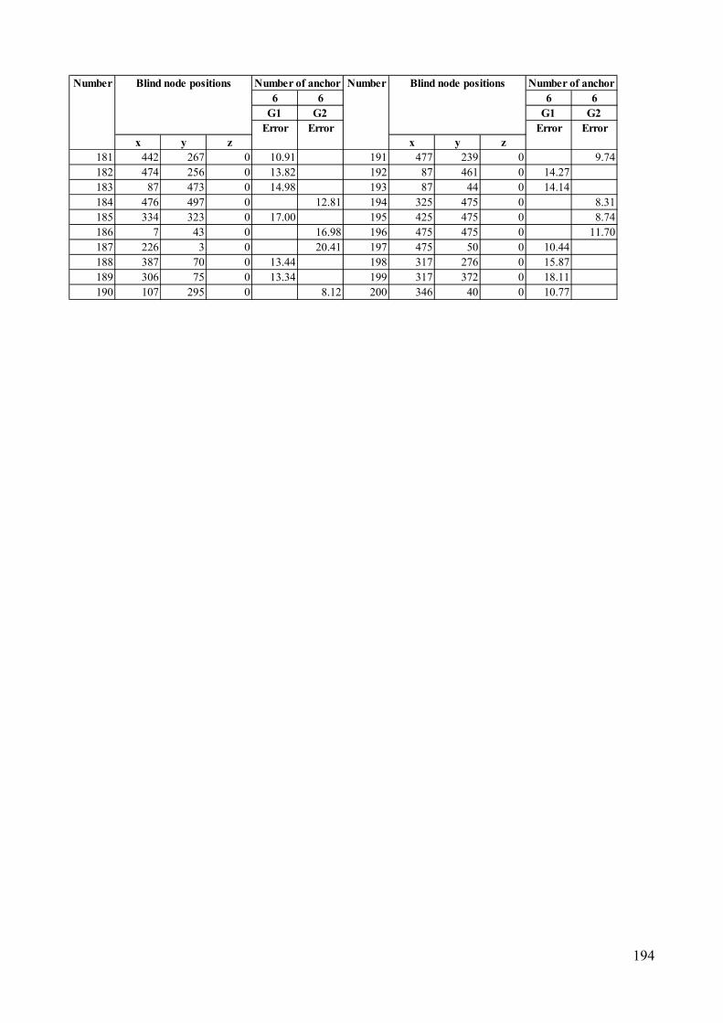
194
6 6 6 6G1 G2 G1 G2
x y z x y z181 442 267 0 10.91 191 477 239 0 9.74182 474 256 0 13.82 192 87 461 0 14.27183 87 473 0 14.98 193 87 44 0 14.14184 476 497 0 12.81 194 325 475 0 8.31185 334 323 0 17.00 195 425 475 0 8.74186 7 43 0 16.98 196 475 475 0 11.70187 226 3 0 20.41 197 475 50 0 10.44188 387 70 0 13.44 198 317 276 0 15.87189 306 75 0 13.34 199 317 372 0 18.11190 107 295 0 8.12 200 346 40 0 10.77
Blind node positions Number of anchor
Error Error
Number Blind node positions Number of anchor
Error Error
Number

195
2) Localization of 200 blind nodes using 7 anchor positions.
7 7 7 7 7 7G1 G2 G3 G1 G2 G3
x y z x y z1 319 228 0 13.73 41 166 64 0 14.042 232 12 0 25.96 42 166 488 0 19.363 481 439 0 10.74 43 244 330 0 14.324 251 92 0 10.18 44 315 287 0 14.145 96 19 0 9.45 45 399 278 0 9.086 420 240 0 18.36 46 223 289 0 14.807 222 253 0 10.92 47 454 206 0 13.238 281 275 0 8.08 48 482 334 0 9.479 87 340 0 9.14 49 463 449 0 9.00
10 390 43 0 15.13 50 454 172 0 10.7711 207 424 0 15.00 51 342 494 0 16.8212 114 111 0 17.08 52 66 85 0 7.2113 22 481 0 19.92 53 361 129 0 15.4714 385 111 0 12.67 54 55 198 0 7.0715 247 140 0 9.19 55 59 37 0 6.9516 165 101 0 10.62 56 320 342 0 12.0817 442 9 0 12.59 57 164 201 0 8.8318 235 91 0 10.77 58 327 491 0 15.3919 130 296 0 15.84 59 375 201 0 19.2620 231 198 0 10.63 60 292 310 0 9.4321 37 46 0 10.77 61 370 77 0 5.4222 208 284 0 16.16 62 117 191 0 15.6023 265 179 0 13.30 63 367 81 0 18.5524 362 388 0 12.60 64 485 379 0 9.2525 26 269 0 7.81 65 433 436 0 7.0726 384 302 0 13.75 66 43 175 0 12.1727 363 377 0 11.35 67 183 343 0 7.1428 448 342 0 9.06 68 185 147 0 11.9829 356 427 0 15.26 69 343 265 0 8.9930 321 437 0 8.74 70 299 416 0 12.5231 384 264 0 10.98 71 395 299 0 9.1132 349 394 0 10.00 72 184 168 0 13.8033 102 321 0 7.28 73 103 150 0 9.5334 80 33 0 9.00 74 43 226 0 10.7235 393 84 0 6.32 75 386 211 0 14.2136 169 397 0 15.62 76 103 180 0 16.7637 299 20 0 12.82 77 194 279 0 17.2938 336 99 0 13.59 78 276 371 0 16.0339 215 32 0 15.56 79 114 212 0 13.6840 291 385 0 11.40 80 321 215 0 18.01
Number Blind node positions Number of anchor positions
Error ErrorError
Number Blind node positions Number of anchor positions
Error Error Error

196
7 7 7 7 7 7G1 G2 G3 G1 G2 G3
x y z x y z81 242 62 0 14.54 131 350 262 0 12.1082 76 12 0 20.12 132 57 404 0 9.6983 391 145 0 11.44 133 25 30 0 19.6584 50 159 0 9.67 134 265 82 0 9.9285 147 327 0 12.21 135 266 221 0 8.8386 119 478 0 13.09 136 471 189 0 9.8587 265 468 0 13.09 137 206 183 0 9.7288 46 229 0 12.92 138 162 381 0 11.6689 203 120 0 20.44 139 249 216 0 9.9290 52 382 0 8.06 140 348 484 0 19.2491 56 380 0 13.23 141 419 488 0 6.8992 177 358 0 142 143 334 0 12.5893 486 428 0 17.72 143 41 100 0 8.8594 173 141 0 16.22 144 50 277 0 10.9295 443 366 0 15.81 145 394 100 0 10.9396 227 69 0 146 420 482 0 12.0497 207 418 0 11.22 147 123 415 0 14.6498 109 69 0 12.12 148 125 25 0 12.8199 63 294 0 10.59 149 134 98 0 13.91
100 154 183 0 22.47 150 348 297 0 9.37101 99 200 0 6.20 151 242 110 0 7.07102 188 87 0 8.71 152 423 76 0 12.42103 439 88 0 18.00 153 95 335 0 15.68104 144 403 0 7.55 154 484 152 0 22.44105 254 230 0 12.06 155 252 206 0 19.34106 315 423 0 13.78 156 479 22 0 16.76107 388 430 0 16.56 157 200 253 0 15.82108 133 13 0 8.77 158 205 108 0 10.54109 124 166 0 18.44 159 411 318 0 13.80110 248 409 0 7.18 160 417 147 0 8.06111 48 425 0 13.30 161 375 15 0 11.11112 59 371 0 12.88 162 24 243 0 14.87113 285 260 0 9.24 163 218 300 0 12.73114 206 142 0 9.22 164 450 90 0 10.74115 454 166 0 17.53 165 187 123 0 16.88116 1 286 0 10.98 166 84 493 0 13.38117 192 492 0 24.19 167 447 341 0 11.55118 103 153 0 12.60 168 222 469 0 8.64119 17 75 0 15.43 169 389 252 0 11.71120 245 203 0 9.33 170 171 147 0 14.57121 466 388 0 12.27 171 313 17 0 9.53122 106 292 0 8.06 172 338 114 0 15.81123 48 267 0 14.23 173 398 303 0 16.40124 253 340 0 15.26 174 124 439 0 18.20125 190 56 0 7.94 175 270 237 0 17.18126 249 130 0 14.28 176 433 260 0 11.25127 111 418 0 11.43 177 94 474 0 10.81128 461 370 0 7.21 178 475 170 0 13.34129 48 481 0 11.25 179 41 38 0 11.96130 305 23 0 19.24 180 98 268 0 22.33
Blind node positions Number of anchor positions
Error Error
Number
Error
Number Blind node positions Number of anchor positions
Error Error Error

197
7 7 7 7 7 7G1 G2 G3 G1 G2 G3
x y z x y z181 442 267 0 10.74 191 477 239 0 24.28182 474 256 0 27.02 192 87 461 0 10.72183 87 473 0 16.15 193 87 44 0 11.87184 476 497 0 11.72 194 325 475 0 17.57185 334 323 0 8.91 195 425 475 0 13.90186 7 43 0 13.04 196 475 475 0 18.44187 226 3 0 13.34 197 475 50 0 11.25188 387 70 0 13.90 198 317 276 0 7.62189 306 75 0 15.40 199 317 372 0 8.03190 107 295 0 9.68 200 346 40 0 10.05
Blind node positions Number of anchor positions
Error Error
Number
Error
Number Blind node positions Number of anchor positions
Error Error Error

198
3) Localization of 200 blind nodes using 8 anchor positions.
8 8 8 8 8 8 8 8 8 8G1 G2 G3 G4 G5 G1 G2 G3 G4 G5
x y z x y z1 319 228 0 13.40 61 370 77 0 5.832 232 12 0 17.80 62 117 191 0 13.103 481 439 0 16.7 63 367 81 0 11.184 251 92 0 9.22 64 485 379 0 13.905 96 19 0 17.17 65 433 436 0 13.566 420 240 0 11.35 66 43 175 0 7.817 222 253 0 10.59 67 183 343 0 11.318 281 275 0 10.25 68 185 147 0 14.149 87 340 0 15.13 69 343 265 0 12.77
10 390 43 0 12.10 70 299 416 0 14.1411 207 424 0 13.60 71 395 299 0 10.9312 114 111 0 12.27 72 184 168 0 15.4413 22 481 0 15.77 73 103 150 0 10.5314 385 111 0 13.17 74 43 226 0 13.0015 247 140 0 10.74 75 386 211 0 11.5816 165 101 0 19.57 76 103 180 0 13.6717 442 9 0 21.56 77 194 279 0 17.8018 235 91 0 11.09 78 276 371 0 11.1819 130 296 0 14.02 79 114 212 0 17.5920 231 198 0 13.80 80 321 215 0 11.2921 37 46 0 9.90 81 242 62 0 10.3022 208 284 0 11.74 82 76 12 0 14.3523 265 179 0 10.00 83 391 145 0 9.6324 362 388 0 16.98 84 50 159 0 11.0925 26 269 0 20.00 85 147 327 0 12.4526 384 302 0 12.19 86 119 478 0 13.227 363 377 0 15.52 87 265 468 0 6.0828 448 342 0 14.28 88 46 229 0 12.1829 356 427 0 12.37 89 203 120 0 13.1930 321 437 0 14.64 90 52 382 0 11.7031 384 264 0 13.8 91 56 380 0 9.2232 349 394 0 11.24 92 177 358 0 15.0833 102 321 0 12.65 93 486 428 0 17.634 80 33 0 16.75 94 173 141 0 10.4435 393 84 0 14.87 95 443 366 0 13.6636 169 397 0 9.0 96 227 69 0 10.8937 299 20 0 13.00 97 207 418 0 22.438 336 99 0 12.21 98 109 69 0 12.7339 215 32 0 15.2 99 63 294 0 14.1840 291 385 0 11.87 100 154 183 0 14.0241 166 64 0 13.34 101 99 200 0 13.0042 166 488 0 19.3 102 188 87 0 9.7143 244 330 0 14.00 103 439 88 0 11.1144 315 287 0 16.02 104 144 403 0 17.2245 399 278 0 14.78 105 254 230 0 17.4946 223 289 0 12.18 106 315 423 0 12.6047 454 206 0 11.14 107 388 430 0 14.2348 482 334 0 19.05 108 133 13 0 18.7949 463 449 0 21.20 109 124 166 0 10.1550 454 172 0 9.49 110 248 409 0 10.4451 342 494 0 8.9 111 48 425 0 19.6552 66 85 0 21.54 112 59 371 0 10.6353 361 129 0 12.73 113 285 260 0 10.9154 55 198 0 13.04 114 206 142 0 14.9555 59 37 0 12.21 115 454 166 0 9.7456 320 342 0 13.23 116 1 286 0 14.457 164 201 0 14.23 117 192 492 0 12.158 327 491 0 16.6 118 103 153 0 11.6659 375 201 0 12.8 119 17 75 0 14.8160 292 310 0 10.14 120 245 203 0 13.30
Blind node positions
Error Error Error
Number Number of anchor positions
Error Error Error
Number Blind node positions Number of anchor positions
Error Error Error Error

199
8 8 8 8 8 8 8 8 8 8G1 G2 G3 G4 G5 G1 G2 G3 G4 G5
x y z x y z121 466 388 0 14.32 161 375 15 0 17.0122 106 292 0 11.79 162 24 243 0 12.7123 48 267 0 15.0 163 218 300 0 3.16124 253 340 0 10.72 164 450 90 0 10.59125 190 56 0 12.45 165 187 123 0 13.96126 249 130 0 14.11 166 84 493 0 11.72127 111 418 0 14.1 167 447 341 0 13.73128 461 370 0 8.00 168 222 469 0 11.43129 48 481 0 14.9 169 389 252 0 9.33130 305 23 0 14.76 170 171 147 0 14.38131 350 262 0 14.59 171 313 17 0 16.97132 57 404 0 12.10 172 338 114 0 14.37133 25 30 0 22.2 173 398 303 0 20.42134 265 82 0 13.28 174 124 439 0 10.03135 266 221 0 17.35 175 270 237 0 14.59136 471 189 0 13.42 176 433 260 0 10.25137 206 183 0 14.23 177 94 474 0 13.9138 162 381 0 18.44 178 475 170 0 11.66139 249 216 0 9.22 179 41 38 0 10.43140 348 484 0 17.0 180 98 268 0 14.23141 419 488 0 16.1 181 442 267 0 8.00142 143 334 0 11.87 182 474 256 0 19.85143 41 100 0 8.03 183 87 473 0 19.00144 50 277 0 14.71 184 476 497 0 18.14145 394 100 0 13.68 185 334 323 0 17.26146 420 482 0 20.5 186 7 43 0 16.8147 123 415 0 10.63 187 226 3 0 17.1148 125 25 0 17.18 188 387 70 0 9.45149 134 98 0 15.00 189 306 75 0 13.25150 348 297 0 17.33 190 107 295 0 11.18151 242 110 0 12.78 191 477 239 0 13.89152 423 76 0 8.25 192 87 461 0 16.1153 95 335 0 12.52 193 87 44 0 16.49154 484 152 0 17.1 194 325 475 0 11.5155 252 206 0 12.99 195 425 475 0 16.65156 479 22 0 17.0 196 475 475 0 15.59157 200 253 0 9.92 197 475 50 0 16.05158 205 108 0 12.81 198 317 276 0 21.21159 411 318 0 1.41 199 317 372 0 12.73160 417 147 0 10.98 200 346 40 0 10.41
Blind node positions
Error Error Error
Number Number of anchor positions
Error Error Error
Number Blind node positions Number of anchor positions
Error Error Error Error

200
Appendix F
F.1. Experiment using edge path planning. See section 8.3.2.
1) Localization error for 200 blind nodes using edge path planning.
x y z x y z x y z PL1 9 228 0 6.50 0 250 10 77 28
0 200 10 78 3035 261 0 83 4245 206 0 84 4551 231 0 84 4550 200 13 86 51
2 232 12 0 8.27 250 0 10 71 18200 0 10 77 28200 25 0 83 42265 50 0 83 42220 56 0 86 51228 50 0 86 51
3 481 439 0 16.76 449 430 04 251 92 0 11.40 250 100 10 65 12
220 56 0 78 30200 100 10 84 45250 50 13 85 48200 50 13 86 51300 100 10 86 51
5 96 19 0 13.96 99 33 06 420 240 0 15.27 430 245 07 222 253 08 281 275 09 87 340 0 9.55 84 349 0 62 10
100 350 10 68 1581 316 0 75 2457 361 0 79 3250 350 13 81 37
100 400 10 82 39
10 390 43 0 13.59 408 47 011 207 424 0 7.14 200 450 13 76 26
200 400 10 76 26250 400 10 76 26208 465 0 81 37250 450 13 82 39150 400 10 87 55
12 114 111 0 12.51 100 100 10 72 20158 116 0 73 2183 160 0 82 39
150 100 10 83 42100 75 0 83 42162 119 0 84 45
13 22 481 0 12.86 22 484 014 385 111 0 15.95 371 116 015 247 140 016 165 101 0 20.62 158 116 0
Error Mobile anchor + Local anchor Estimated distance
Number Blind node positions Number of anchor positions6 6
G1 G2Error Local anchor from G1

201
17 442 9 0 10.27 450 0 10 67 14460 25 0 74 23450 50 13 79 32408 47 0 80 34500 0 10 83 42400 0 10 85 48
18 235 91 0 16.74 250 100 10 66 13228 50 0 78 30250 50 13 79 32220 56 0 80 34162 119 0 81 37200 50 13 84 45
19 130 296 020 231 198 021 37 46 0 13.60 37 48 022 208 284 023 265 179 024 362 388 0 15.08 356 388 025 26 269 0 13.15 35 261 026 384 302 0 20.95 400 300 10 70 17
410 307 0 76 26400 250 10 85 48430 245 0 85 48350 357 0 88 59450 300 13 89 63
27 363 377 0 15.44 350 357 028 448 342 0 15.06 455 342 029 356 427 0 12.73 382 432 030 321 437 0 14.40 300 450 13 69 16
350 450 13 78 30300 400 10 80 34382 432 0 86 51350 400 10 87 55400 400 10 88 59
31 384 264 0 29.57 400 250 10 72 20430 245 0 84 45410 307 0 84 45450 250 13 87 55400 300 10 87 55450 200 13 88 59
32 349 394 0 19.00 345 386 033 102 321 0 14.95 100 300 10 73 21
81 316 0 73 21100 350 10 79 3284 349 0 79 3257 273 0 82 39
146 359 0 83 42
34 80 33 0 11.11 56 22 035 393 84 0 16.87 393 100 036 169 397 0 34.53 170 389 037 299 20 0 12.45 290 29 038 336 99 0 20.61 333 122 039 215 32 0 18.72 200 25 040 291 385 0 7.50 300 400 10 67 21
250 400 10 72 21350 357 0 83 32246 417 0 84 32250 450 13 85 39356 388 0 87 42
41 166 64 0 16.58 162 59 0
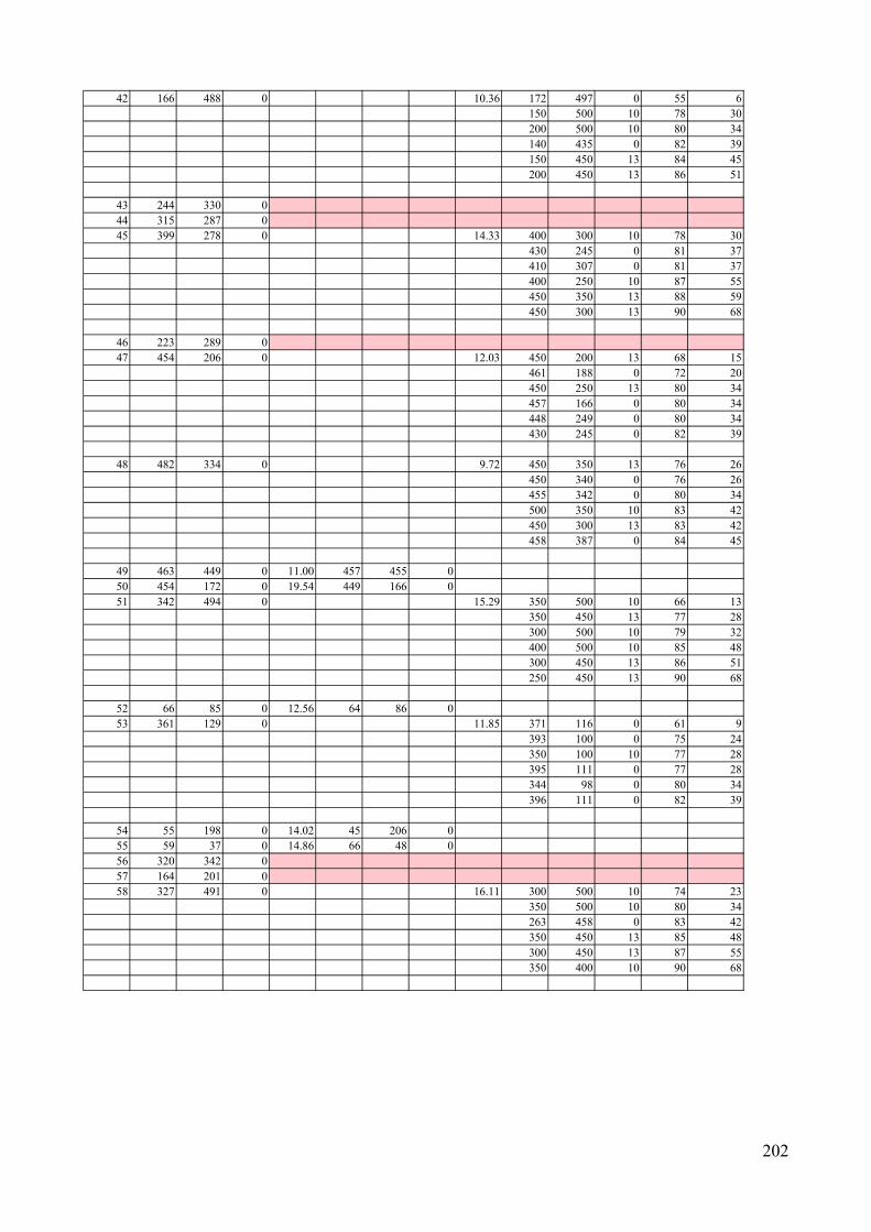
202
42 166 488 0 10.36 172 497 0 55 6150 500 10 78 30200 500 10 80 34140 435 0 82 39150 450 13 84 45200 450 13 86 51
43 244 330 044 315 287 045 399 278 0 14.33 400 300 10 78 30
430 245 0 81 37410 307 0 81 37400 250 10 87 55450 350 13 88 59450 300 13 90 68
46 223 289 047 454 206 0 12.03 450 200 13 68 15
461 188 0 72 20450 250 13 80 34457 166 0 80 34448 249 0 80 34430 245 0 82 39
48 482 334 0 9.72 450 350 13 76 26450 340 0 76 26455 342 0 80 34500 350 10 83 42450 300 13 83 42458 387 0 84 45
49 463 449 0 11.00 457 455 050 454 172 0 19.54 449 166 051 342 494 0 15.29 350 500 10 66 13
350 450 13 77 28300 500 10 79 32400 500 10 85 48300 450 13 86 51250 450 13 90 68
52 66 85 0 12.56 64 86 053 361 129 0 11.85 371 116 0 61 9
393 100 0 75 24350 100 10 77 28395 111 0 77 28344 98 0 80 34396 111 0 82 39
54 55 198 0 14.02 45 206 055 59 37 0 14.86 66 48 056 320 342 057 164 201 058 327 491 0 16.11 300 500 10 74 23
350 500 10 80 34263 458 0 83 42350 450 13 85 48300 450 13 87 55350 400 10 90 68

203
59 375 201 060 292 310 061 370 77 0 25.75 381 102 062 117 191 0 23.60 100 200 10 72 20
100 150 10 85 4883 160 0 85 4850 150 13 87 5550 200 13 87 5545 206 0 87 55
63 367 81 0 23.78 361 83 064 485 379 0 11.99 456 376 0 73 21
500 400 10 74 23458 387 0 77 28455 342 0 79 32450 367 0 79 32450 340 0 80 34
65 433 436 0 8.98 432 443 066 43 175 0 13.30 48 167 067 183 343 068 185 147 069 343 265 070 299 416 0 8.64 300 400 10 64 11
300 450 13 80 34350 400 10 82 39200 400 10 85 48350 357 0 87 55246 417 0 87 55
71 395 299 0 15.66 410 307 0 63 11400 300 10 65 12450 250 13 85 48400 250 10 85 48450 300 13 86 51400 350 10 86 51
72 184 168 073 103 150 0 22.20 83 160 074 43 226 0 16.65 51 231 0 60 9
45 206 0 74 2350 250 13 77 2850 200 13 78 300 200 10 79 32
35 261 0 79 32
75 386 211 076 103 180 0 7.11 100 200 10 78 30
100 150 10 83 42100 250 10 84 4551 231 0 84 4550 200 13 86 5157 273 0 86 51
77 194 279 078 276 371 079 114 212 0 24.63 100 200 10 72 20
100 250 10 83 4269 232 0 85 4845 206 0 86 51
100 150 10 87 5550 200 13 89 63
80 321 215 081 242 62 0 10.51 220 56 082 76 12 0 18.41 78 1 0
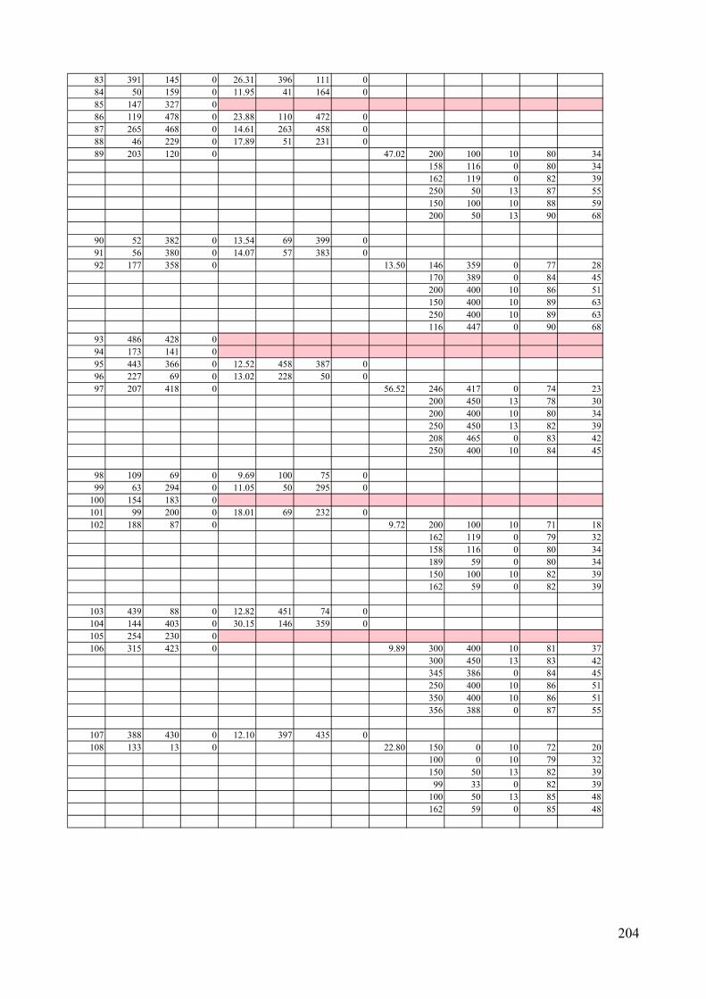
204
83 391 145 0 26.31 396 111 084 50 159 0 11.95 41 164 085 147 327 086 119 478 0 23.88 110 472 087 265 468 0 14.61 263 458 088 46 229 0 17.89 51 231 089 203 120 0 47.02 200 100 10 80 34
158 116 0 80 34162 119 0 82 39250 50 13 87 55150 100 10 88 59200 50 13 90 68
90 52 382 0 13.54 69 399 091 56 380 0 14.07 57 383 092 177 358 0 13.50 146 359 0 77 28
170 389 0 84 45200 400 10 86 51150 400 10 89 63250 400 10 89 63116 447 0 90 68
93 486 428 094 173 141 095 443 366 0 12.52 458 387 096 227 69 0 13.02 228 50 097 207 418 0 56.52 246 417 0 74 23
200 450 13 78 30200 400 10 80 34250 450 13 82 39208 465 0 83 42250 400 10 84 45
98 109 69 0 9.69 100 75 099 63 294 0 11.05 50 295 0
100 154 183 0101 99 200 0 18.01 69 232 0102 188 87 0 9.72 200 100 10 71 18
162 119 0 79 32158 116 0 80 34189 59 0 80 34150 100 10 82 39162 59 0 82 39
103 439 88 0 12.82 451 74 0104 144 403 0 30.15 146 359 0105 254 230 0106 315 423 0 9.89 300 400 10 81 37
300 450 13 83 42345 386 0 84 45250 400 10 86 51350 400 10 86 51356 388 0 87 55
107 388 430 0 12.10 397 435 0108 133 13 0 22.80 150 0 10 72 20
100 0 10 79 32150 50 13 82 3999 33 0 82 39
100 50 13 85 48162 59 0 85 48

205
109 124 166 0 5.83 100 150 10 74 2383 160 0 81 37
100 200 10 84 4541 164 0 87 55
158 116 0 88 5948 167 0 88 59
110 248 409 0 41.11 246 417 0111 48 425 0 14.25 58 449 0112 59 371 0 13.15 57 361 0113 285 260 0114 206 142 0 12.22 162 119 0 82 39
200 100 10 83 42150 100 10 87 55250 100 10 87 55158 116 0 87 55220 56 0 89 63
115 454 166 0 10.00 457 166 0116 1 286 0 9.87 0 300 10 71 18
0 250 10 76 2635 261 0 78 3057 273 0 84 4550 300 13 85 4850 295 0 87 55
117 192 492 0 9.85 172 497 0118 103 153 0 19.34 59 159 0119 17 75 0 21.32 42 73 0120 245 203 0121 466 388 0 7.79 450 367 0122 106 292 0 37.34 81 316 0123 48 267 0 11.43 57 273 0124 253 340 0125 190 56 0 14.40 189 59 0126 249 130 0127 111 418 0 22.50 99 453 0128 461 370 0 8.38 456 376 0129 48 481 0 12.65 43 467 0130 305 23 0 7.84 300 0 10 70 17
313 34 0 70 17290 29 0 78 30300 50 13 79 32350 0 10 81 37344 40 0 82 39
131 350 262 0132 57 404 0 15.70 56 394 0133 25 30 0 9.89 20 30 0134 265 82 0 22.52 265 50 0135 266 221 0136 471 189 0 17.80 461 188 0137 206 183 0138 162 381 0 16.70 170 389 0 60 9
150 400 10 74 23146 359 0 84 45200 400 10 89 6350 400 13 90 6857 361 0 90 68
139 249 216 0140 348 484 0141 419 488 0 22.55 409 465 0

206
142 143 334 0 17.54 170 389 0 66 13146 359 0 75 24150 400 10 77 28200 400 10 82 39100 400 10 86 51116 447 0 88 59
143 41 100 0 8.85 37 100 0144 50 277 0 12.62 57 273 0 62 10
35 261 0 72 2050 250 13 74 2350 295 0 74 2369 232 0 82 3950 300 13 83 42
145 394 100 0 12.17 395 111 0146 420 482 0 17.09 443 479 0147 123 415 0 25.74 140 435 0148 125 25 0 11.48 100 0 10 74 23
99 33 0 75 24150 50 13 79 32150 0 10 82 39100 50 13 86 51100 75 0 86 51
149 134 98 0 21.48 162 119 0150 348 297 0 25.18 310 318 0 82 39
350 357 0 83 42400 300 10 84 45400 250 10 86 51345 386 0 89 63450 340 0 90 68
151 242 110 0 23.08 250 100 10 66 13200 100 10 83 42189 59 0 85 48220 56 0 86 51250 50 13 88 59300 100 10 88 59
152 423 76 0 14.97 429 80 0153 95 335 0 23.41 84 349 0154 484 152 0 19.01 500 150 10 71 18
457 166 0 75 24437 154 0 79 32496 181 0 79 32461 188 0 80 34500 200 10 81 37
155 252 206 0156 479 22 0 9.88 460 25 0157 200 253 0158 205 108 0 15.52 200 100 10 66 13
158 116 0 81 37162 119 0 82 39189 59 0 85 48250 100 10 86 51220 56 0 86 51

207
159 411 318 0 17.06 410 307 0160 417 147 0 11.50 437 154 0161 375 15 0 20.59 380 -25 0162 24 243 0 7.07 35 261 0 69 16
45 206 0 75 240 250 10 78 30
51 231 0 79 3257 273 0 80 3450 250 13 82 39
163 218 300 0164 450 90 0 8.06 452 88 0165 187 123 0 23.84 200 100 10 72 20
162 119 0 77 28150 100 10 82 39150 50 13 86 51158 116 0 86 51189 59 0 87 55
166 84 493 0 15.41 106 468 0 71 18100 500 10 75 24110 472 0 75 2450 500 10 80 3450 450 13 82 3943 467 0 85 48
167 447 341 0 8.56 450 340 0168 222 469 0 14.00 208 465 0169 389 252 0 18.23 400 250 10 61 9
430 245 0 78 30448 249 0 83 42410 307 0 88 59450 250 13 89 63400 200 10 90 68
170 171 147 0 52.80 150 100 10 83 42200 100 10 85 48158 116 0 85 48100 150 10 87 55162 119 0 87 55189 59 0 89 63
171 313 17 0 20.38 313 34 0172 338 114 0 10.06 344 98 0173 398 303 0 11.65 400 300 10 63 11
410 307 0 64 11430 245 0 85 48400 250 10 88 59400 350 10 88 59350 357 0 88 59
174 124 439 0 7.67 116 447 0175 270 237 0176 433 260 0 9.84 430 245 0 66 13
448 249 0 68 15450 250 13 73 21400 300 10 80 34450 300 13 84 45400 250 10 84 45
177 94 474 0 9.90 106 468 0178 475 170 0 24.27 496 181 0179 41 38 0 10.02 24 24 0

208
180 98 268 0 12.80 57 273 0 74 23100 250 10 75 2450 295 0 82 3950 250 13 83 42
100 300 10 84 4550 300 13 87 55
181 442 267 0 15.95 448 249 0182 474 256 0 9.76 500 250 10 76 26
448 249 0 78 30430 245 0 79 32450 250 13 81 37410 307 0 86 51500 300 10 87 55
183 87 473 0 15.57 62 457 0184 476 497 0 13.52 474 509 0185 334 323 0186 7 43 0 13.38 20 45 0187 226 3 0 12.53 200 0 10 73 21
250 0 10 78 30228 50 0 79 32200 25 0 84 45220 56 0 85 48200 50 13 87 55
188 387 70 0 15.24 395 60 0189 306 75 0 9.71 300 100 10 72 20
300 50 13 78 30344 98 0 79 32265 50 0 80 34250 100 10 81 37290 29 0 82 39
190 107 295 0 18.57 100 300 10 70 1781 316 0 77 2857 273 0 79 3250 250 13 85 48
100 350 10 85 4884 349 0 85 48
191 477 239 0 10.12 500 250 10 71 18448 249 0 79 32450 250 13 81 37450 200 13 83 42500 200 10 84 45430 245 0 84 45
192 87 461 0 13.95 85 433 0193 87 44 0 13.29 78 55 0194 325 475 0195 425 475 0 18.83 408 460 0196 475 475 0 7.91 461 467 0197 475 50 0 6.16 475 46 0198 317 276 0199 317 372 0 14.13 300 400 10 77 28
356 388 0 77 28345 386 0 77 28350 357 0 80 34310 318 0 85 48350 400 10 86 51
200 346 40 0 17.03 344 40 0