1

Localization of Wireless Sensor Networks in theWild: Pursuit of Ranging Quality

Jizhong Zhao, Member, IEEE, Wei Xi, Student Member, IEEE, Yuan He Member, IEEE, YunhaoLiu, Senior Member, IEEE, XiangYang Li, Senior Member, IEEE, Lufeng Mo, Member, IEEE, Zheng

Yang, Member, IEEE,

Abstract—Localization is a fundamental issue of wireless sensor networks that has been extensively studied in the literature. Ourreal-world experience from GreenOrbs, a sensor network system deployed in a forest, shows that localization in the wild remains verychallenging due to various interfering factors. In this paper we propose CDL, a Combined and Differentiated Localization approachfor localization that exploits the strength of range-free approaches and range-based approaches using RSSI. A critical observation isthat ranging quality greatly impacts the overall localization accuracy. To achieve a better ranging quality, our method CDL incorporatesvirtual-hop localization, local filtration, and ranging-quality aware calibration. We have implemented and evaluated CDL by extensivereal-world experiments in GreenOrbs and large-scale simulations. Our experimental and simulation results demonstrate that CDLoutperforms current state-of-art localization approaches with a more accurate, and consistent performance. For example, the averagelocation error using CDL in GreenOrbs system is 2.9m, while the previous best method SISR has an average error of 4.6m.

Index Terms—Localization, Wireless Sensor Network, RSSI, Ranging Quality.

✦

1 INTRODUCTION

LOCALIZATION is crucial for many services pro-vided by wireless sensor networks (WSNs), which

has received substantive attention in recent years. TheGlobal Positioning System (GPS) are popular localizationschemes, but usually fail to function indoors [11], underthe ground [10], or in forests with dense canopies [14].Range-based approaches measure the Euclidean dis-tances among the nodes with various ranging techniques[16], [20], [24]. They are either expensive with respect tohardware cost, or susceptible to environmental noisesand dynamics [23]. Range-free approaches perform lo-calization by relying only on network connectivity mea-surements. However, localization results by range-freeapproaches are typically imprecise and easily affectedby node density.

This work is motivated by the need for accurate loca-tion information in GreenOrbs [14], a large-scale sensornetwork system deployed in a forest. An indispensableelement in various GreenOrbs applications is the locationinformation of sensor nodes for purposes such as firerisk evaluation, canopy closure estimates, microclimateobservation, and search and rescue in the wild. Our real-world experiences of GreenOrbs reveal that localization

• Wei Xi, Jizhong Zhao, Lufeng Mo are with Xi’An Jiaotong University.• Yuan He and Zheng Yang are with the Tsinghua National Laboratory for

Information Science and Technology, Tsinghua University.• Yunhao Liu is with the School of Software and TNLIST, Tsinghua

University, and also with the Hong Kong University of Science andTechnology.

• XiangYang Li is with Department of Computer Science, Illinois Instituteof Technology.

• The preliminary result was published at ACM SenSys 2010.

in the wild remains very challenging, in spite of greatefforts and results developed in the literature. The chal-lenges come from various aspects. First, non-uniform de-ployment of sensor nodes could affect the effectivenessof range-free localization. On the other hand, for range-based localization, the received signal strength indicators(RSSIs) used for estimating distances are highly irregular,dynamic, and asymmetric between pairs of nodes. Tomake it even worse, the complex terrain and obstacles inthe forest easily affect RSSI-based range measurements,thus incurring undesired but ubiquitous errors.

Ranging based localization techniques often producesbetter localization than range-free techniques. Rang-ing quality determines the overall localization accuracy.Bearing this in mind, recently proposed approaches fo-cused more on error control and management. Someof those methods enhance the localization accuracy bydeliberately reducing the contribution of error-pronenodes to the localization process [13]. Other schemes areto identify large ranging errors and outliers relying ontopological or geometric properties of a network [7], [27].

Ranging quality indeed includes two aspects. Oneof them refers to the location accuracy of the refer-ence nodes. The other concerns the accuracy of rangemeasurements. Both aspects play important roles onthe accuracy of localization. Most of the recently pro-posed techniques address only one aspect, thus failingto achieve satisfactory accuracy.

To address these challenges and limitations, we pro-pose CDL, a Combined and Differentiated Localizationapproach. CDL inherits the advantages of both range-free and range-based methods. It starts from a coarse-grained localization achieved by method such as DV-

2

hop, and then it keeps improving the ranging qualityand localization accuracy iteratively throughout the lo-calization process. The contributions of this work aresummarized as follows.

1) We propose a range-free scheme called virtual-hoplocalization, which makes full use of local informa-tion to mitigate the non-uniform node distributionproblem. Using virtual-hop, the initial estimatedlocations are more accurate than those output byother range-free schemes.

2) To improve the ranging quality, we design twolocal filtration techniques, namely neighborhood hop-count matching and neighborhood sequence matching,to find nodes with better location accuracy. Thefiltered good nodes can be used to improve thelocation accuracy of neighboring nodes.

3) Using the good nodes to calibrate the bad ones, weemploy the weighted robust estimation to empha-size contributions of the best range measurements,eliminate the interfering outliers, and suppress theimpact of ranges in-between.

4) We implement CDL in GreenOrbs system withmore than 300 sensor nodes deployed in a forestand evaluate it with extensive experiments andlarge-scale simulations. Our experimental and sim-ulation results demonstrate that CDL outperformsexisting approaches with high accuracy, efficiency,and consistent performance. For example, the aver-age location error using CDL in GreenOrbs systemis 2.9m, while the previous best method SISR hasan average error of 4.6m.

The rest of this paper is organized as follows. Section 2briefly reviews the related work. Section 3 presents real-world observations on GreenOrbs. The design of CDL iselaborated in Section 4, followed by performance evalu-ation in Section 5. We conclude the paper in Section 6.

2 RELATED WORK

The existing work on localization falls into two maincategories: range-based and range-free localization.

Range-free approaches, such as Centroid [2], APIT [5],and DV-HOP [17], mainly rely on connectivity measure-ments (for example hop-count) from landmarks to theother nodes. Since the quality of localization is easilyaffected by node density and network conditions, range-free approaches typically provide imprecise estimationof node locations. Range-based approaches measure theEuclidean distances among the nodes with certain rang-ing techniques and locate the nodes using geometricmethods, such as TOA [1], TDOA [18], [20], and AOA[16]. All those approaches require extra hardware sup-port.

RSSI-based range measurements are easy-to-implement and popular in practice. Empirical modelsof signal propagation are constructed to convert RSSIto distance [21]. The accuracy of such conversions,however, is sensitive to channel noise, interference, and

multipath effects. Besides, when there are a limitednumber of landmarks, range-based approaches have toundergo iterative calculation processes to locate all thenodes, suffering significant accumulative errors [13].

More recent proposals mainly focus on the issue oferror control and management [12], [26]. J. Liu et al. [13]propose iterative localization with error management.Only a portion of nodes are selected into localization,based on their relative contribution to the localizationaccuracy, so as to avoid error accumulation during theiterations. Similarly, H.T. Kung et al. [8] propose to assigndifferent weights to range measurements with differentnodes and adopt a robust statistical technique to tolerateoutliers of range measurements [7].

A range-free approach beyond connectivity is pro-posed in [27]. The signature distance is proposed as ameasure of the Euclidean distance between a pair ofnodes. In order to address the issue of non-uniform de-ployment, the authors further propose regulated signaturedistance (RSD), which takes node density into account.Based on the comparison among nodes’ neighbor se-quences, RSD is quantified. This approach needs to beintegrated with a certain existing localization approachto function.

Differing with most of the existing approaches, CDLis a combination of range-free and range-based schemes.It can independently localize a WSN. CDL addressesthe issue of non-uniform deployment with virtual-hoplocalization (Subsection 4.1). Utilizing the informationof estimated node locations, RSSI readings, and networkconnectivity, CDL filters good nodes from bad ones withtwo techniques (Subsection 4.2), namely neighborhoodhop-count matching and neighborhood sequence match-ing. CDL pursues better ranging quality (namely moreaccurate reference locations and more accurate ranging)throughout the localization process. This is the mostsignificant characteristic of CDL that distinguishes itfrom existing approaches.

For ease of presentation, we use the terms “rang-ing” and “range measurement”, “location” and “coordi-nates”, interchangeably throughout the rest of this paper.

3 PRELIMINARY AND DESIGN MOTIVATION

3.1 GreenOrbs

GreenOrbs is an ongoing research project that aimsat building long-term large-scale WSN systems in theforest. It adopts TelosB motes with MSP430 processorand CC2420 radio. The software running on the nodesis developed based on TinyOS 2.1. There are 330 nodesin a deployment area of about 40, 000m2. The majorityof Greenorbs nodes should be deployed where environ-mental information is required by forestry applications.The rest are used to improve network connectivity.

The collected data can be utilized to support a widevariety of applications, e.g. distance-dependent compe-tition measurement for predicting growth of individualtrees, light detection and ranging to characterize forest

3

Fig. 1: GreenOrbs deployment in the campus woodland

stand condition, and percentage estimation of groundarea vertically shaded by overhead foliage. These appli-cations generally require accurate coordinates of sensornodes’ locations to provide high-quality information ofthe forest [9], [14], [25].

This work is carried out in GreenOrbs. The ground-truth coordinates of the nodes are measured usingan EDM (Electronic Distance Measuring Device) [3].The measurement process is hence laborious and time-consuming. So far we have succeeded in measuringthe coordinates of 100 nodes, as shown in Fig. 1. Theobservations and experiments in this paper are thenmainly conducted using those 100 nodes. The other 230nodes, although deployed in an adjacent area, are notshown in the figure.

3.2 Observations

As shown in Fig. 1, most sensor nodes are under densetree cover, where GPS usually does not work [1]. Evenin areas with less dense tree cover, our experience showsthat the errors produced by a portable GPS device(compared to an EDM) are often about 15m. Thus lo-cating nodes basically comes down to in-network local-ization. This subsection presents real-world observationson GreenOrbs, which illustrate that a single approach,whether it is range-based or range-free, has limitationsin locating a number of nodes in the wild.

3.2.1 Non-uniform Deployment

Driven by forestry applications, GreenOrbs deploysmore sensor nodes in regions with diverse or unevenvegetation to provide fine-grained information of themonitored area. Such a rule leads to non-uniform de-ployment of sensor nodes, as we can see from Fig. 1.Specifically, some nodes have more than 20 neighbors,while some nodes have less than 5 neighbors. Theshortest distance is 5m and the longest is around 108m.Range-free localization in a non-uniform deploymentoften incurs large errors.

3.2.2 Irregularity of RSSI

Besides the non-uniform deployment problem, complexterrain and obstacles (e.g. shrubs and tree trunks) alsoaffect signal propagation in the forest. Fig. 2 plots theRSSI between node pairs in GreenOrbs at a certain time.It also includes a curve, which shows the mapping

0 10 20 30 40 50 60 70 80 90−95

−90

−85

−80

−75

−70

−65

Distance Between Node Pairs (m)

RS

SI (

dBm

)

Fig. 2: RSSI of differentnode pairs

0 5 10 15 20−95

−90

−85

−80

−75

Time (hour)

RS

SI (

dBm

)

RSSI from B to ARSSI from A to B

Fig. 3: RSSI between nodesA and B over time

between RSSI and the distance based on the log normalshadowing model, see Equation (1).

PL(d) = PL(d0)− 10× η × log(d

d0) +Xσ (1)

where PL(d) denotes the reduction in received signalstrength after propagating through a distance d, PL(d0)stands for the path loss at a short reference distance d0,η is the path loss factor (also named signal propagationconstant), and Xσ is a random environment noise fol-lowing X∼N(0, σX2) reported in [19].

We can see that the real distances between node pairsdiffer greatly from the model-based estimations. Thoughthe mapping between the RSSI and the distance is actu-ally very uncertain, RSSI still offers useful information.In most cases, a stronger RSSI corresponds to a shorterdistance, as is also observed in [4], [27].

3.2.3 Asymmetry and Dynamics of RSSIFig. 3 shows the RSSI of two directed links AB andBA between two nodes A and B in GreenOrbs overtime. The distance between A and B is 41.27 meters. Wecan see that the RSSI between two nodes is asymmetric.Two pairwise links often have unequal RSSI. Moreover,RSSI is often susceptible to environmental factors, suchas humidity and temperature. The RSSI over a directedlink also fluctuates over time.

In summary, we have the following important ob-servations on GreenOrbs. First, the sensor nodes aredeployed with diverse densities in different regions,causing the non-uniform distribution problem. Second,RSSI is very unstable and sensitive to various environ-mental factors. The uncertainty of RSSI is hard to modelin practice, therefore, RSSI-based range measurementsexhibit quite diverse errors. To make matters even worse,typically only large ranging errors can be detected ortolerated by the existing approaches.

4 CDL DESIGN

We consider locating a network of wireless nodes on atwo dimensional plane by using the connectivity infor-mation and RSSI readings. A few nodes, which knowtheir own coordinates once they are deployed, are usedas landmarks. The design of CDL mainly consists ofvirtual-hop localization, local filtration, and ranging-qualityaware calibration. Fig. 4 illustrates the CDL workflow.

4

3. Ranging-quality

Aware Calibration2. Local Filtration

Neighborhood Hop-

count Matching

Neighborhood

Sequence Matching

Judgment

1. Virtual-hop

Localization

Be a

reference

Calibration

Do nothing

Good

Bad

Undertermined

Fig. 4: The workflow of CDL

Virtual-hop localization initially estimates node locationsusing a range-free method. In order to approximatethe distances from each node to the landmarks, we leteach node count the virtual-hops instead of DV-hops,compensating particularly for the errors caused by thenon-uniform deployment problem.

Subsequently, CDL executes an iterative process offiltration and calibration. In each filtration step, CDL usestwo filtering methods to identify good nodes whose lo-cation accuracy is already satisfactory. Neighborhood hop-count matching filters the bad nodes by verifying a node’shop-counts to its neighbors. Furthermore, neighborhoodsequence matching distinguishes good nodes from badones by contrasting two sequences on each node. Eachsequence sorts a node’s neighbors using a particularmetric, such as RSSI and estimated distance.

Those identified good nodes are regarded as refer-ences and used to calibrate the location of bad ones.Links with different ranging quality are given differentweights. Outliers in range measurements are toleratedusing robust estimation.

In the next three subsections, we elaborate on thedesign of the above three phases respectively.

4.1 Virtual-Hop Localization

For the first phase of CDL, virtual-hop localization ini-tially computes node locations. This is an enhanced ver-sion of hop-count based localization. Compared to theDV-hop scheme, virtual-hop particularly addresses theissue of non-uniform deployment. Based on the outputof virtual-hop localization, the subsequent localizationprocesses in CDL (filtration and calibration) are expectedto achieve higher accuracy and efficiency of iteration.

4.1.1 Weakness of Range-free localization algorithm

As analyzed in [15], there is a theoretical limitationon range-free localization algorithm that is based onlyon connectivity. Suppose sensor nodes are randomlydistributed in the monitoring area. Each sensor can beregarded as a node in a graph, so that two nodes areconnected by an edge if and only if they can communi-cate with each other in one hop, i.e. they are less than thedistance r from each other. It is possible to move a sensornode over nonzero distance without changing the set ofits one-hop neighbors. The original and moved locationsof nodes are indistinguishable from the point of view

r

d k i

(a) (b)

Fig. 5: Intuition of virtual-Hop distance: (a) cumulativedistribution of node distances, (b) relationship among

neighbors with different hop counts.

of the network connectivity. The average Euclidean dis-tance between its original location and a moved locationthat does not changing the network connectivity gives alower bound on the expected resolution achievable.

As shown in Fig. 5(a), a sensor node can be moveddistance d without changing the connectivity, if there isno sensor in the shaded area.

Nagpal et al. [15] have claimed that rπ/4nlocal is theexpected lower bound for the error in any range-freelocalization algorithm in static sensor networks wherenlocal is the connectivity degree, and the nodes only usethe connectivity information of the seeds within theirfirst-hop neighborhoods.

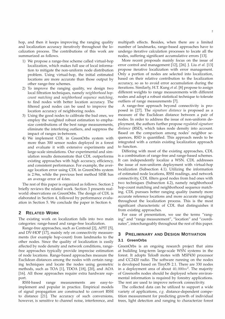
DV-hop is one of the common range-free localiza-tion approaches that utilize connectivity informationto estimate node locations. Every node counts its hopcounts to landmarks. The distance between a node anda landmark is calculated as the product of the hop countbetween them and the per-hop distance, which is a pre-determined constant for all the nodes. The location ofa node is calculated by using Least Squares Estimation.However, nodes with the same hop often have quite dif-ferent distances to landmarks. Fig. 6 shows some nodesthat are within three hops away from the landmark. Forexample, nodes va and vb are both two hops away fromlandmark Rk, while va is closer to landmark than vb.A constant value of per-hop distance for every nodeoften causes errors on distance calculation from a nodeto landmarks. As a result, the localization accuracy ofDV-hop is far from satisfactory.

4.1.2 Virtual-hop

Since traditional hop-count based technology doesn’tdifferentiate two distances with the same hop counts, wepropose a metric virtual-hop-count, Vjk , to represent thedistance between an ordinary node vj and a landmarkRk. Among the nodes with the same hop count to Rk,node closer to Rk should have a smaller Vjk . For easeof presentation, Table 1 lists the symbols and notationsused in this paper. Each node vj computes its Vjk by

Vjk =1

|Pjk|

∑

vi∈Pjk

Vik + Ljk (2)

5

va

vb

Rk r

r

First hop

Second hop

Third hop

Fig. 6: The same hop counts have different distances

TABLE 1: Symbols and notations

Symbol Definitionhij hop count from node vi to node vjVjk virtual-hop-count from landmark Rk to node vjℜj {vi

∣

∣hij = 1}Pjk {vi

∣

∣hij = 1 and hki < hkj}Njk {vi

∣

∣hij = 1 and hki > hkj}ζjk min{|Pik|

∣

∣ vi is in Njk}ϕjk min{|Nik|

∣

∣ vi is in Pjk}

where

Ljk =

|Njk|

|Njk|+ ζjk − 1, |Njk| > 0

ϕjk

|Pjk|+ ϕjk − 1, |Njk| = 0

Vjk consists of two parts: The first part is the averagevirtual-hop-count of node vj ’s previous-hop neighbors.The second part is the last virtual-hop-count, that is,the incremental virtual-hop-count from vj ’s previous-hop neighbors to vj , denoted by Ljk . Here, a nodevj ’s previous-hop neighbor is defined as a neighboringnode whose hop count to landmark Rk is just one hopless than vj , (denoted by Pjk in Table 1). vj ’s next-hopneighbor is defined as a neighboring node whose hopcount is just one hop more than vj (denoted by Njk inTable 1).

We now explain the intuition behind our definitionof virtual-hop-count using probability analysis. Fig. 5(b)shows the relationship among neighbors with differenthop counts. The concentric circles separately denote thelocation boundary of one-hop, two-hops and three-hopsneighbors of landmark Rk. The dashed circle denotes thecommunication range of vi who is a two-hops neighborof Rk. The intersection, denoted as A(Pik), of dashedcircle and small circle (centered at Rk) is the regionwhere vi’ previous-hop neighbors locate. The intersec-tion, denoted as A(Nik), of the dashed circle and the bigcircle centered at Rk is the region where vi’s next-hopneighbors could locate.

For any node vi, as long as the distance between itand landmark Rk (denoted by d) satisfies r < d < 2r,it has two hops to Rk. In this case, the maximumresidual of two distances with the same hop count isclose to r. For virtual-hop, such two nodes have differentvirtual-hop-counts. For ease of explanation, we assumeconnectivity degree is nlocal and calculate the residualof node vi’s last virtual-hop-count to Rk denoted by

0 20 40 60 80 1000

5

10

15

20

25

30

Node ID

Loca

lizat

ion

Err

or (

m)

DV−hop Virtual−hop

Fig. 7: Virtual-hop VS DV-hop

0 20 40 60 80 1000

10

20

30

40

Node ID

Loca

lizat

ion

Err

or (

m)

Virtual−hopIndiscriminate Calibration

Fig. 8: Indiscriminate Cal-ibration

Lik defined in Equation 2. The closer vi is to Rk, thelarger the area of A(Pik), and smaller Lik is, while DV-hop has a constant hop count. The maximum value ofLik is close to 1. The minimum value of Lik is closeto 1

ζik= 1/[nlocal

πr2

∫ Y

0(√

4r2 − y2 − 2r +√

r2 − y)dy] ≈π/1.4nlocal. The upper bound for expected ranging errorof DV-hop is r, while the bound for virtual-hop isπr/1.4nlocal. Therefore, virtual-hop can reduce both theupper bound and average of localization error whennlocal is greater than 3.

Let R be the set of landmarks in the sensor networkwhose exact positions are known in advance. Let ρtk bethe Euclidean distance between landmarks Rt and Rk.The per-virtual-hop distance, denoted as d̃k, regardinglandmark Rk is calculated by

d̃k =

∑

Rt∈R ρtk∑

Rt∈R Vtk

(3)

Each node vj without known location then estimates itsdistance, denoted as ρjk , to each landmark Rk by

ρjk = d̃k · Vjk (4)

After calculating the distances to landmarks, each nodecomputes its coordinates based on trilateration usingLeast Square Estimation (LSE), which is similar to DV-hop.

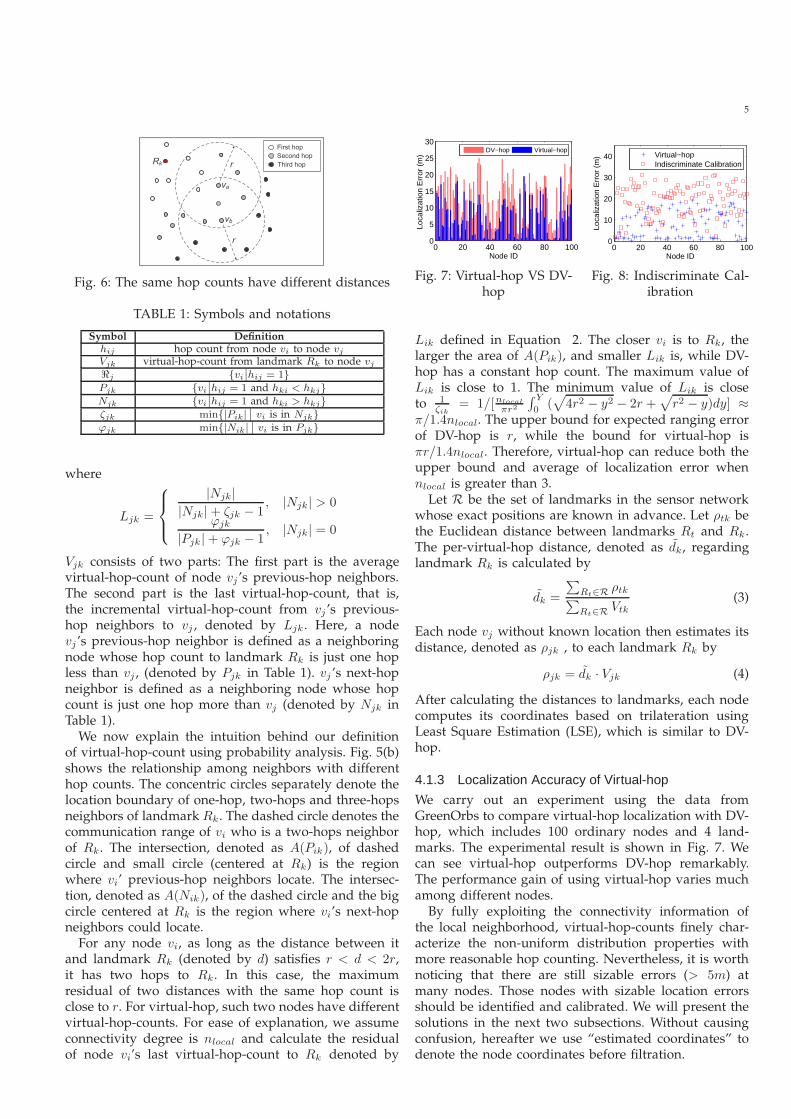
4.1.3 Localization Accuracy of Virtual-hop

We carry out an experiment using the data fromGreenOrbs to compare virtual-hop localization with DV-hop, which includes 100 ordinary nodes and 4 land-marks. The experimental result is shown in Fig. 7. Wecan see virtual-hop outperforms DV-hop remarkably.The performance gain of using virtual-hop varies muchamong different nodes.

By fully exploiting the connectivity information ofthe local neighborhood, virtual-hop-counts finely char-acterize the non-uniform distribution properties withmore reasonable hop counting. Nevertheless, it is worthnoticing that there are still sizable errors (> 5m) atmany nodes. Those nodes with sizable location errorsshould be identified and calibrated. We will present thesolutions in the next two subsections. Without causingconfusion, hereafter we use “estimated coordinates” todenote the node coordinates before filtration.

6

(a)

vd

vc

vb

vevf

vg

va

va'

(b)

Fig. 9: ADM reflects the localization error of a node

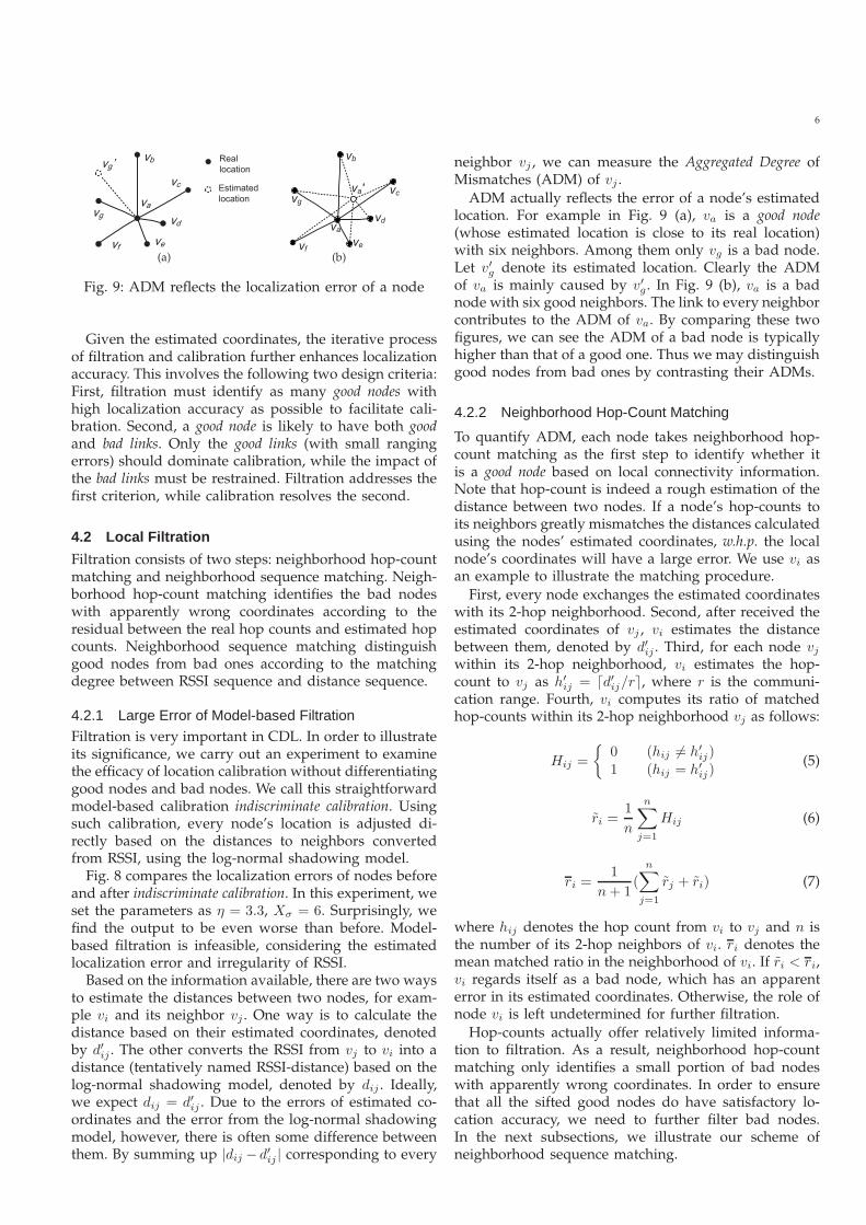
Given the estimated coordinates, the iterative processof filtration and calibration further enhances localizationaccuracy. This involves the following two design criteria:First, filtration must identify as many good nodes withhigh localization accuracy as possible to facilitate cali-bration. Second, a good node is likely to have both goodand bad links. Only the good links (with small rangingerrors) should dominate calibration, while the impact ofthe bad links must be restrained. Filtration addresses thefirst criterion, while calibration resolves the second.

4.2 Local Filtration

Filtration consists of two steps: neighborhood hop-countmatching and neighborhood sequence matching. Neigh-borhood hop-count matching identifies the bad nodeswith apparently wrong coordinates according to theresidual between the real hop counts and estimated hopcounts. Neighborhood sequence matching distinguishgood nodes from bad ones according to the matchingdegree between RSSI sequence and distance sequence.

4.2.1 Large Error of Model-based FiltrationFiltration is very important in CDL. In order to illustrateits significance, we carry out an experiment to examinethe efficacy of location calibration without differentiatinggood nodes and bad nodes. We call this straightforwardmodel-based calibration indiscriminate calibration. Usingsuch calibration, every node’s location is adjusted di-rectly based on the distances to neighbors convertedfrom RSSI, using the log-normal shadowing model.

Fig. 8 compares the localization errors of nodes beforeand after indiscriminate calibration. In this experiment, weset the parameters as η = 3.3, Xσ = 6. Surprisingly, wefind the output to be even worse than before. Model-based filtration is infeasible, considering the estimatedlocalization error and irregularity of RSSI.

Based on the information available, there are two waysto estimate the distances between two nodes, for exam-ple vi and its neighbor vj . One way is to calculate thedistance based on their estimated coordinates, denotedby d′ij . The other converts the RSSI from vj to vi into adistance (tentatively named RSSI-distance) based on thelog-normal shadowing model, denoted by dij . Ideally,we expect dij = d′ij . Due to the errors of estimated co-ordinates and the error from the log-normal shadowingmodel, however, there is often some difference betweenthem. By summing up |dij − d′ij | corresponding to every

neighbor vj , we can measure the Aggregated Degree ofMismatches (ADM) of vj .

ADM actually reflects the error of a node’s estimatedlocation. For example in Fig. 9 (a), va is a good node(whose estimated location is close to its real location)with six neighbors. Among them only vg is a bad node.Let v′g denote its estimated location. Clearly the ADMof va is mainly caused by v′g . In Fig. 9 (b), va is a badnode with six good neighbors. The link to every neighborcontributes to the ADM of va. By comparing these twofigures, we can see the ADM of a bad node is typicallyhigher than that of a good one. Thus we may distinguishgood nodes from bad ones by contrasting their ADMs.

4.2.2 Neighborhood Hop-Count Matching

To quantify ADM, each node takes neighborhood hop-count matching as the first step to identify whether itis a good node based on local connectivity information.Note that hop-count is indeed a rough estimation of thedistance between two nodes. If a node’s hop-counts toits neighbors greatly mismatches the distances calculatedusing the nodes’ estimated coordinates, w.h.p. the localnode’s coordinates will have a large error. We use vi asan example to illustrate the matching procedure.

First, every node exchanges the estimated coordinateswith its 2-hop neighborhood. Second, after received theestimated coordinates of vj , vi estimates the distancebetween them, denoted by d′ij . Third, for each node vjwithin its 2-hop neighborhood, vi estimates the hop-count to vj as h′

ij = ⌈d′ij/r⌉, where r is the communi-cation range. Fourth, vi computes its ratio of matchedhop-counts within its 2-hop neighborhood vj as follows:

Hij =

{

0 (hij 6= h′ij)

1 (hij = h′ij)

(5)

r̃i =1

n

n∑

j=1

Hij (6)

ri =1

n+ 1(

n∑

j=1

r̃j + r̃i) (7)

where hij denotes the hop count from vi to vj and n isthe number of its 2-hop neighbors of vi. ri denotes themean matched ratio in the neighborhood of vi. If r̃i < ri,vi regards itself as a bad node, which has an apparenterror in its estimated coordinates. Otherwise, the role ofnode vi is left undetermined for further filtration.

Hop-counts actually offer relatively limited informa-tion to filtration. As a result, neighborhood hop-countmatching only identifies a small portion of bad nodeswith apparently wrong coordinates. In order to ensurethat all the sifted good nodes do have satisfactory lo-cation accuracy, we need to further filter bad nodes.In the next subsections, we illustrate our scheme ofneighborhood sequence matching.

7

vg

N a B C D E F G

S a 6 5 1 2 4 3

S a ' 6 4 1 2 3 5

(a)

N a B C D E F G

S a 6 5 1 2 4 3

S a ' 4 2 1 3 6 5

(b)

Fig. 10: Neighborhood sequence matching

4.2.3 Neighborhood Sequence Matching

Though model-based straightforward filtration is infea-sible, RSSI still offers useful information. Generally, theRSSI between two nodes decreases monotonically as thedistance increases observed from the RSSI readings inFig. 2. Based on this observation, we propose a filtrationscheme called neighborhood sequence matching.

First, va sorts its neighbors in descending order withregard to the RSSI from them, generating a sequencenumber for each neighbor. By mapping the sequencenumbers into va, we get the first sequence called RSSIsequence. Let Sa denote it, as illustrated in Fig. 10.

Second, according to the estimated coordinates, vasorts its neighbors in the ascending order with regardto the estimated distance to them, generating the secondsequence called distance sequence. Let S′

a denote it.In environment without noises, Sa and S′

a shouldbe identical. If there is significant mismatch betweenthem, it indicates a large error in the node’s estimatedcoordinates. We use the same examples as that in Fig. 9to illustrate the above idea. As shown in Fig. 10 (a), thereis not a significant mismatch between Sa and S′

a in thiscase. Comparatively in Fig. 10 (b), there appears to besignificant mismatch between Sa and S′

a.Now that the difference between Sa and S′

a is causedby following categories of reasons: the location esti-mation errors, the irregularity of RSSI between va andits neighbors, and the log norm shadowing model forestimating distance using RSSI.

Since the location estimation error is analyzed before,we discuss the influence of the irregularity of RSSI.From the Fig. 2, we can think that RSSI still satisfiesthe property that it decreases with the increase of thedistance between two neighboring nodes.

The next step is to quantify the distance between RSSIsequence and distance sequence to distinguish goodnodes from bad ones. In order to improve the filtrationperformance, we need to suppress the influence of theirregularity of RSSI first.

The cosine distance is a measure of similarity betweentwo vectors by finding the cosine of the angle between

them. It is considered to be used to measure the similar-ity between sequences Sa and S′

a. Given two vectors ofattributes, the cosine distance is represented using a dotproduct and magnitude as following:

CosDist =a1a

′1 + a2a

′2 + ...+ ana

′n

√

a21 + a22 + ...+ a2n√

a′21 + a

′22 + ...+ a′2

n

=a1a

′1 + a2a

′2 + ...+ ana

′n

12 + 22 + ...+ n2

(8)

In Equation (8), a1, a2, ..., an are the sequence numbersin Sa while a′1, a′2, ..., a′n are the sequence numbersin S′

a. These two sequences are actually two differ-ent permutations of 1, 2, ..., n. Thus they are twoequal sets. The cosine distance filtration reduces theinfluence of RSSI irregularity. For example, RSSI se-quence Sa is {6, 5, 1, 2, 4, 3}, and distance sequence S′

a

is {6, 4, 1, 2, 3, 5} as shown in Fig. 10 (a) CosDista isequal to 0.967. As the irregularity, Sa occurs local flipsin the nodes with similar distance such as vd and ve, orvf and vg . It may become {6, 5, 2, 1, 3, 4}, then CosDistabecomes 0.978 which is close to the theoretical value. Thecosine filtration distance has good fault tolerance to sup-press the influence of RSSI irregularity. Upper bound of

CosDist is 1, lower bound is 1·n+2(n−1)+3(n−2)+...+n·112+22+...+n2 =

n+22n+1 , which is not less than 0.5.

However, when a good node has some bad neighborswith large location errors, the cosine distance betweentwo sequences of a good node does not apparently differfrom that of a bad node. To deal with this issue, weintroduce the LCS (longest common subsequence) lengthratio δa. Let n denote the number of va’s neighbors. Thenδa denotes the ratio of the length of the LCS between Sa

and S′a to n. It is easy to see that the LCS length ratio of

a good node is higher than that of a bad node.The LCS length ratio δa is error-tolerant to interference

of bad neighboring nodes with large location estimationerrors. The boundary of δ is between 0 and 1.

We define the matching degree Mi between the RSSIsequence and distance sequence as follows.

Mi = δi · CosDisti (9)

Clearly Mi is a better metric to distinguish good nodesfrom bad nodes. When a small portion of RSSI readingshave relatively large errors, or a good node has somebad neighbors with large location errors, the matchingdegree cannot be influenced too much.

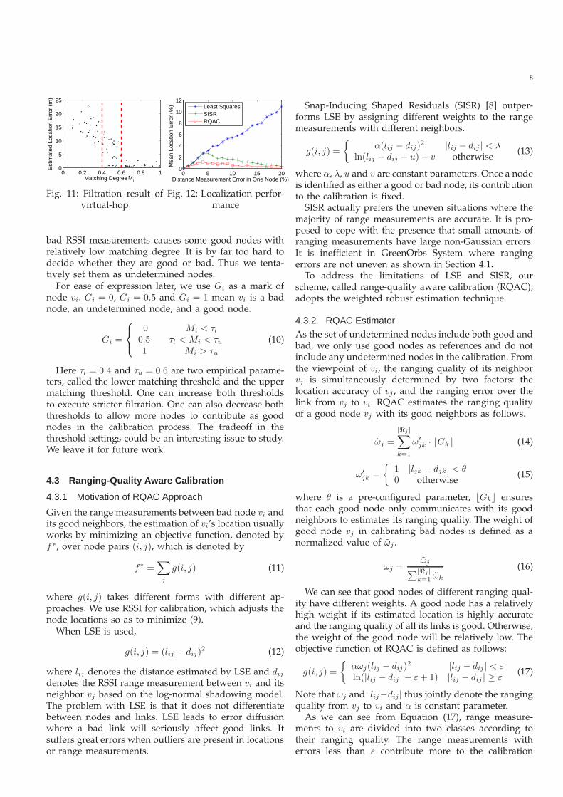
We use the same trace as that in Fig. 7 to calculate thematching degree of all the nodes after initial localization.The results are plotted in Fig. 11. Nodes of a matchingdegree over 0.6 have location errors of less than 4 meters.We regard them as good nodes. Nodes of less than 0.4degree have location errors over 5 meters. We regardthem as bad nodes. The other nodes have matchingdegrees between 0.4 and 0.6, but their location errorsvary from 0.1 to 12 meters. The excessive number ofbad neighbors with large location estimation errors or

8

0 0.2 0.4 0.6 0.8 10

5

10

15

20

25

Matching Degree

Est

imat

ed L

ocat

ion

Err

or (

m)

Mi

Fig. 11: Filtration result ofvirtual-hop

0 5 10 15 200

2

4

6

8

10

12

Distance Measurement Error in One Node (%)

Mea

n Lo

catio

n E

rror

(%

)

Least SquaresSISRRQAC

Fig. 12: Localization perfor-mance

bad RSSI measurements causes some good nodes withrelatively low matching degree. It is by far too hard todecide whether they are good or bad. Thus we tenta-tively set them as undetermined nodes.

For ease of expression later, we use Gi as a mark ofnode vi. Gi = 0, Gi = 0.5 and Gi = 1 mean vi is a badnode, an undetermined node, and a good node.

Gi =

0 Mi < τl0.5 τl < Mi < τu1 Mi > τu

(10)

Here τl = 0.4 and τu = 0.6 are two empirical parame-ters, called the lower matching threshold and the uppermatching threshold. One can increase both thresholdsto execute stricter filtration. One can also decrease boththresholds to allow more nodes to contribute as goodnodes in the calibration process. The tradeoff in thethreshold settings could be an interesting issue to study.We leave it for future work.

4.3 Ranging-Quality Aware Calibration

4.3.1 Motivation of RQAC Approach

Given the range measurements between bad node vi andits good neighbors, the estimation of vi’s location usuallyworks by minimizing an objective function, denoted byf∗, over node pairs (i, j), which is denoted by

f∗ =∑

j

g(i, j) (11)

where g(i, j) takes different forms with different ap-proaches. We use RSSI for calibration, which adjusts thenode locations so as to minimize (9).

When LSE is used,

g(i, j) = (lij − dij)2 (12)

where lij denotes the distance estimated by LSE and dijdenotes the RSSI range measurement between vi and itsneighbor vj based on the log-normal shadowing model.The problem with LSE is that it does not differentiatebetween nodes and links. LSE leads to error diffusionwhere a bad link will seriously affect good links. Itsuffers great errors when outliers are present in locationsor range measurements.

Snap-Inducing Shaped Residuals (SISR) [8] outper-forms LSE by assigning different weights to the rangemeasurements with different neighbors.

g(i, j) =

{

α(lij − dij)2 |lij − dij | < λ

ln(lij − dij − u)− v otherwise(13)

where α, λ, u and v are constant parameters. Once a nodeis identified as either a good or bad node, its contributionto the calibration is fixed.

SISR actually prefers the uneven situations where themajority of range measurements are accurate. It is pro-posed to cope with the presence that small amounts ofranging measurements have large non-Gaussian errors.It is inefficient in GreenOrbs System where rangingerrors are not uneven as shown in Section 4.1.

To address the limitations of LSE and SISR, ourscheme, called range-quality aware calibration (RQAC),adopts the weighted robust estimation technique.

4.3.2 RQAC Estimator

As the set of undetermined nodes include both good andbad, we only use good nodes as references and do notinclude any undetermined nodes in the calibration. Fromthe viewpoint of vi, the ranging quality of its neighborvj is simultaneously determined by two factors: thelocation accuracy of vj , and the ranging error over thelink from vj to vi. RQAC estimates the ranging qualityof a good node vj with its good neighbors as follows.

ω̃j =

|ℜj |∑

k=1

ω′jk · ⌊Gk⌋ (14)

ω′jk =

{

1 |ljk − djk| < θ0 otherwise

(15)

where θ is a pre-configured parameter, ⌊Gk⌋ ensuresthat each good node only communicates with its goodneighbors to estimates its ranging quality. The weight ofgood node vj in calibrating bad nodes is defined as anormalized value of ω̃j .

ωj =ω̃j

∑|ℜj |k=1 ω̃k

(16)

We can see that good nodes of different ranging qual-ity have different weights. A good node has a relativelyhigh weight if its estimated location is highly accurateand the ranging quality of all its links is good. Otherwise,the weight of the good node will be relatively low. Theobjective function of RQAC is defined as follows:

g(i, j) =

{

αωj(lij − dij)2 |lij − dij | < ε

ln(|lij − dij | − ε+ 1) |lij − dij | ≥ ε(17)

Note that ωj and |lij−dij | thus jointly denote the rangingquality from vj to vi and α is constant parameter.

As we can see from Equation (17), range measure-ments to vi are divided into two classes according totheir ranging quality. The range measurements witherrors less than ε contribute more to the calibration

9

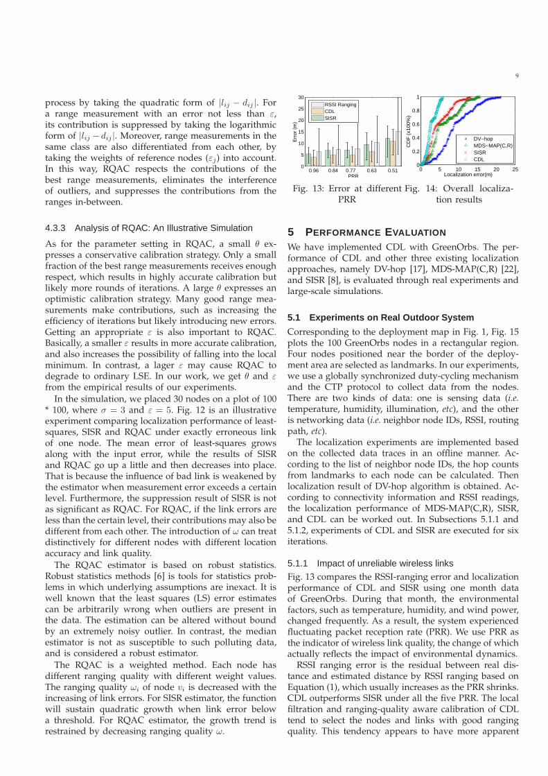
process by taking the quadratic form of |lij − dij |. Fora range measurement with an error not less than ε,its contribution is suppressed by taking the logarithmicform of |lij − dij |. Moreover, range measurements in thesame class are also differentiated from each other, bytaking the weights of reference nodes (εj) into account.In this way, RQAC respects the contributions of thebest range measurements, eliminates the interferenceof outliers, and suppresses the contributions from theranges in-between.

4.3.3 Analysis of RQAC: An Illustrative Simulation

As for the parameter setting in RQAC, a small θ ex-presses a conservative calibration strategy. Only a smallfraction of the best range measurements receives enoughrespect, which results in highly accurate calibration butlikely more rounds of iterations. A large θ expresses anoptimistic calibration strategy. Many good range mea-surements make contributions, such as increasing theefficiency of iterations but likely introducing new errors.Getting an appropriate ε is also important to RQAC.Basically, a smaller ε results in more accurate calibration,and also increases the possibility of falling into the localminimum. In contrast, a lager ε may cause RQAC todegrade to ordinary LSE. In our work, we get θ and εfrom the empirical results of our experiments.

In the simulation, we placed 30 nodes on a plot of 100* 100, where σ = 3 and ε = 5. Fig. 12 is an illustrativeexperiment comparing localization performance of least-squares, SISR and RQAC under exactly erroneous linkof one node. The mean error of least-squares growsalong with the input error, while the results of SISRand RQAC go up a little and then decreases into place.That is because the influence of bad link is weakened bythe estimator when measurement error exceeds a certainlevel. Furthermore, the suppression result of SISR is notas significant as RQAC. For RQAC, if the link errors areless than the certain level, their contributions may also bedifferent from each other. The introduction of ω can treatdistinctively for different nodes with different locationaccuracy and link quality.

The RQAC estimator is based on robust statistics.Robust statistics methods [6] is tools for statistics prob-lems in which underlying assumptions are inexact. It iswell known that the least squares (LS) error estimatescan be arbitrarily wrong when outliers are present inthe data. The estimation can be altered without boundby an extremely noisy outlier. In contrast, the medianestimator is not as susceptible to such polluting data,and is considered a robust estimator.

The RQAC is a weighted method. Each node hasdifferent ranging quality with different weight values.The ranging quality ωi of node vi is decreased with theincreasing of link errors. For SISR estimator, the functionwill sustain quadratic growth when link error belowa threshold. For RQAC estimator, the growth trend isrestrained by decreasing ranging quality ω.

0.510.630.770.840.960

5

10

15

20

25

30

PRR

Err

or (

m)

RSSI RangingCDLSISR

Fig. 13: Error at differentPRR

0 5 10 15 20 250

0.2

0.4

0.6

0.8

1

Localization error(m)

CD

F (

x100

%)

DV−hopMDS−MAP(C,R)SISRCDL

Fig. 14: Overall localiza-tion results

5 PERFORMANCE EVALUATION

We have implemented CDL with GreenOrbs. The per-formance of CDL and other three existing localizationapproaches, namely DV-hop [17], MDS-MAP(C,R) [22],and SISR [8], is evaluated through real experiments andlarge-scale simulations.

5.1 Experiments on Real Outdoor System

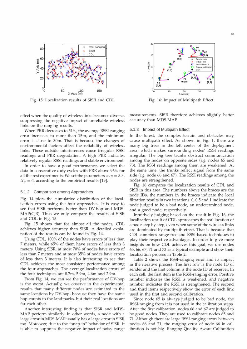
Corresponding to the deployment map in Fig. 1, Fig. 15plots the 100 GreenOrbs nodes in a rectangular region.Four nodes positioned near the border of the deploy-ment area are selected as landmarks. In our experiments,we use a globally synchronized duty-cycling mechanismand the CTP protocol to collect data from the nodes.There are two kinds of data: one is sensing data (i.e.temperature, humidity, illumination, etc), and the otheris networking data (i.e. neighbor node IDs, RSSI, routingpath, etc).

The localization experiments are implemented basedon the collected data traces in an offline manner. Ac-cording to the list of neighbor node IDs, the hop countsfrom landmarks to each node can be calculated. Thenlocalization result of DV-hop algorithm is obtained. Ac-cording to connectivity information and RSSI readings,the localization performance of MDS-MAP(C,R), SISR,and CDL can be worked out. In Subsections 5.1.1 and5.1.2, experiments of CDL and SISR are executed for sixiterations.

5.1.1 Impact of unreliable wireless links

Fig. 13 compares the RSSI-ranging error and localizationperformance of CDL and SISR using one month dataof GreenOrbs. During that month, the environmentalfactors, such as temperature, humidity, and wind power,changed frequently. As a result, the system experiencedfluctuating packet reception rate (PRR). We use PRR asthe indicator of wireless link quality, the change of whichactually reflects the impact of environmental dynamics.

RSSI ranging error is the residual between real dis-tance and estimated distance by RSSI ranging based onEquation (1), which usually increases as the PRR shrinks.CDL outperforms SISR under all the five PRR. The localfiltration and ranging-quality aware calibration of CDLtend to select the nodes and links with good rangingquality. This tendency appears to have more apparent

10

0 50 100 1500

20

40

60

80

X Axis (m)

Y A

xis

(m)

Real LocationSISRCDL

Fig. 15: Localization results of SISR and CDL

effect when the quality of wireless links becomes diverse,suppressing the negative impact of unreliable wirelesslinks on the ranging results.

When PRR decreases to 51%, the average RSSI-rangingerror increases to more than 15m, and the minimumerror is close to 30m. That is because the changes ofenvironmental factors affect the reliability of wirelesslinks. These outside interferences cause irregular RSSIreadings and PRR degradation. A high PRR indicatesrelatively regular RSSI readings and stable environment.

In order to have a good performance, we select thedata in consecutive duty cycles with PRR above 96% forall the rest experiments. We set the parameters as η = 3.3,Xσ = 6, according to the empirical results [19].

5.1.2 Comparison among Approaches

Fig. 14 plots the cumulative distribution of the local-ization errors using the four approaches. It is easy tosee that SISR performs better than DV-hop and MDS-MAP(C,R). Thus we only compare the results of SISRand CDL in Fig. 15.

Fig. 15 shows that for almost all the nodes, CDLachieves higher accuracy than SISR. A detailed expla-nation of the results can be found in Fig. 14.

Using CDL, 100% of the nodes have errors of less than7 meters, while 65% of them have errors of less than 3meters. Using SISR, at most 70% of nodes have errors ofless than 7 meters and at most 35% of nodes have errorsof less than 3 meters. It is also interesting to see thatCDL achieves the most consistent performance amongthe four approaches. The average localization errors ofthe four techniques are 8.7m, 5.9m, 4.6m and 2.9m.

From Fig. 14, we can see the performance of DV-hopis the worst. Actually, we observe in the experimentalresults that many different nodes are estimated to thesame locations by DV-hop, because they have the samehop-counts to the landmarks, but their real locations arefar each other.

Another interesting finding is that SISR and MDS-MAP perform similarly. In other words, a node with alarge error in MDS-MAP usually has a large error in SISRtoo. Moreover, due to the “snap-in” behavior of SISR, itis able to suppress the negative impact of noisy range

0 10 20 30 400

5

10

15

20

X Axis(m)

Y A

xis(

m)

Ground truthVirtual−hopFirst calibrationSecond calibrationSISR

63(0,1)

64 (1,1)

65(0,0)

66(0,1)

67(0,1)

71(0.5,0)

73(1,1)

74(1,1)

Fig. 16: Impact of Multipath Effect

measurements. SISR therefore achieves slightly betteraccuracy than MDS-MAP.

5.1.3 Impact of Multipath EffectIn the forest, the complex terrain and obstacles maycause multipath effect. As shown in Fig. 1, there aremany big trees in the left center of the deploymentarea, which makes surrounding nodes’ RSSI readingsirregular. The big tree trunks obstruct communicationamong the nodes on opposite sides (e.g. nodes 65 and73). The RSSI readings among them are weakened. Atthe same time, the trunks reflect signal from the sameside (e.g. node 66 and 67). The RSSI readings among thenodes are strengthened.

Fig. 16 compares the localization results of CDL andSISR in this area. The numbers above the braces are thenode IDs, the numbers in the braces indicate the localfiltration results in two iterations. 0, 0.5 and 1 indicate thenode judged to be a bad node, an undetermined node,and a good node, respectively.

Intuitively judging based on the result in Fig. 16, thelocalization result of CDL approaches the real location ofa node step by step, even when some of the wireless linksare dominated by multipath effect. That is because thatCDL combines range-free and RSSI-based techniques toplay their respective advantages. In order to give moreinsights on how CDL achieves this goal, we use nodes65, 66, 67, 71 and 73 as a typical example and show theirlocalization process in Table 2.

Table 2 shows the RSSI-ranging error and its impactin the iterative process. The first row is the node ID ofsender and the first column is the node ID of receiver. Ineach cell, the first item is the RSSI-ranging error. Positivenumber indicates the RSSI is weakened, and negativenumber indicates the RSSI is strengthened. The secondand third items respectively show the error of each linkused in the first and second calibration.

Since node 65 is always judged to be bad node, theRSSI-ranging from it is not used in the calibration steps.After the first calibration, nodes 66 and 67 are judged tobe good nodes. They are used to calibrate nodes 65 and71. Although there are large RSSI-ranging errors betweennodes 66 and 71, the ranging error of node 66 in cal-ibration is not big. Ranging-Quality Aware Calibration

11

TABLE 2: RSSI-ranging error and its impact (m)

65 66 67 71 7365 -4.81, 0, -1.43 -2.77, 0, -0.92 10.34, 0, 0 10.87, 1.87, 1.6566 -5.43, 0, 0 -4.85, 0, 0 8.49, 0, 0 5.21, 1.46, 067 -2.51, 0, 0 -4.22, 0, 0 1.63, 0, 0 -0.93, -0.97, 071 11.74, 0, 0 11.55, 0, 2.04 2.37, 0, 0.93 -2.14, 0, -0.7973 11.26, 0, 0 5.37, 0, 0 -0.65, 0, 0 -2.78, 0, 0

(RQAC) can limit the influence of large ranging errorwith the weighted robust estimator.

Overall, the node with bad ranging quality will eitherbe judged to be a bad node during local filtration orbe suppressed with respect to its weight in calibrationby RQAC. Thus, CDL can deal with the local multipatheffect well.

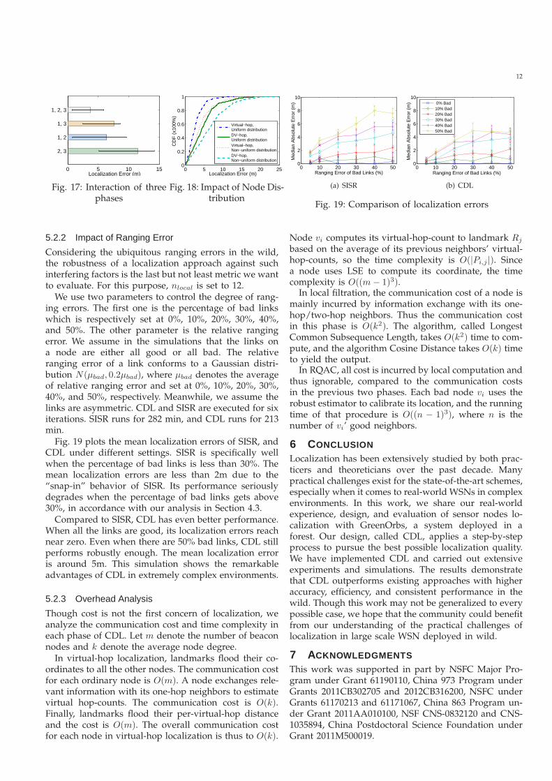
5.1.4 Interaction of Three Phases

CDL mainly consists of three phases: virtual-hop localiza-tion, local filtration, and ranging-quality aware calibration.Fig. 17 shows how these methods interact with eachother. To simplify the notations, we use the numbers 1, 2,3 to represent the three phases. Then there are four kindsof combinations: (2 ∪ 3), (1 ∪ 2), (1 ∪ 3), and (1 ∪ 2 ∪ 3).The different bars indicate the mean localization errorsof different combinations.

For (2 ∪ 3), we use DV-hop instead of virtual-hop toinitialize locations of ordinary nodes. This combinationhas large localization errors. That is because DV-hopinitializes many nodes’ locations to be far away fromtheir real locations. Then good nodes and bad nodes,good links and bad links, cannot be easily differenti-ated. It has serious impact upon the local filtration andranging-quality aware calibration, and finally reducesthe localization accuracy. From this we can see thegreat importance of virtual-hop in CDL, which providesaccurate initial localization.

For (1 ∪ 2), we use Least Squares Estimate instead ofRQAC for calibration. This combination has higher accu-racy than (2∪3). That is because virtual-hop localizationprovides accurate localization for most nodes. In thissituation, nodes can be properly distinguished as goodnodes or bad ones. Meanwhile, it has larger maximumerror than (1∪3). That is because Least Squares Estimatealgorithm leads to error propagation when there aresome bad links. It indicates that it is meaningful andbeneficial to differentiate the ranging quality of differentlinks in the calibration phase.

For (1 ∪ 3), we use RQAC to directly calibrate eachnode without local filtration. This combination has largerminimum error than (1∪2). Without distinguishing goodnodes from bad nodes, it’s difficult to evaluate the rang-ing quality due to the interference of bad nodes. Withoutappropriate differentiation, the good nodes’ locationsare also calibrated by their neighbors, as reduces thelocalization accuracy of good nodes. It indicates thatthe negative impact of bad nodes may be serious andcannot be neglected. In order to achieve highly accurate

localization in the end, we need to filter the bad nodesfirst before entering the calibration phase.

5.2 Simulation on Large Scale Networks

Besides the above experiments, we further carry outextensive simulations to evaluate the performance ofCDL. We examine the location accuracy of CDL bytuning a series of parameters such as network topology,connectivity degree and the relative ranging errors. Theresults of DV-hop, MDS-MAP(C,R), and SISR are pre-sented as well. The simulations run on Matlab, including1000 ordinary nodes in a square region and 6 landmarksaround. We run all the simulations on a Windows 7PC with an Intel i5 2.53GHz processor and two corememories size of 2 Gbytes.

In the simulation setting of Section 5.2.1, each nodehas 10 to 12 neighbors for uniform distribution, andhas 3 to 15 neighbors for non-uniform distribution. InSection 5.2.2 and 5.2.3, nodes are randomly distributedin a square region. Each node’s RSSI readings from itsneighboring nodes are assigned with values based onthe log normal shadowing model with random noise, tobe more close to the real fact. Two nodes are connectedwith a link in the network, if the RSSI between them isgreater than -87dBm (the receiving sensitivity of CC2420radio). In this way, the network topology is generated.

5.2.1 Impact of Network Topology

Virtual-hop is a range-free localization which utilizesthe connectivity information to locate sensor nodes.We examine the performance of virtual-hop in bothscenarios with uniform distribution and non-uniformdistribution. DV-hop algorithm takes 43 seconds to runin either uniform or non-uniform distribution simula-tions. Virtual-hop takes 57 seconds to run in uniformdistribution simulation and 58 seconds to run in non-uniform distribution simulation.

Fig. 18 compares the performance of virtual-hop andDV-hop localization approaches in both scenarios. Theresults indicate that the non-uniform deployment ofnodes does build up the average localization errorsfor both two approaches. It is worth noticing thateven virtual-hop localization in the non-uniform deploy-ment is more accurate than the performance of DV-hop localization in the uniform deployment. DV-hopdoesn’t differentiate between two distances with thesame hop count to landmark, while virtual-hop-countassigns small values to the near nodes.

12

0 5 10 15

2, 3

1, 2

1, 3

1, 2, 3

Localization Error (m)

Fig. 17: Interaction of threephases

0 5 10 15 20 250

0.2

0.4

0.6

0.8

1

Localization Error (m)C

DF

(x1

00%

)

Virtual−hop,Uniform distributionDV−hop,Uniform distributionVirtual−hop,Non−uniform distributionDV−hop,Non−uniform distribution

Fig. 18: Impact of Node Dis-tribution

0 10 20 30 40 500

2

4

6

8

10

Ranging Error of Bad Links (%)

Med

ian

Abs

olut

e E

rror

(m

)

(a) SISR

0 10 20 30 40 500

2

4

6

8

10

Ranging Error of Bad Links (%)

Med

ian

Abs

olut

e E

rror

(m

)

0% Bad10% Bad20% Bad30% Bad40% Bad50% Bad

(b) CDL

Fig. 19: Comparison of localization errors

5.2.2 Impact of Ranging Error

Considering the ubiquitous ranging errors in the wild,the robustness of a localization approach against suchinterfering factors is the last but not least metric we wantto evaluate. For this purpose, nlocal is set to 12.

We use two parameters to control the degree of rang-ing errors. The first one is the percentage of bad linkswhich is respectively set at 0%, 10%, 20%, 30%, 40%,and 50%. The other parameter is the relative rangingerror. We assume in the simulations that the links ona node are either all good or all bad. The relativeranging error of a link conforms to a Gaussian distri-bution N(µbad, 0.2µbad), where µbad denotes the averageof relative ranging error and set at 0%, 10%, 20%, 30%,40%, and 50%, respectively. Meanwhile, we assume thelinks are asymmetric. CDL and SISR are executed for sixiterations. SISR runs for 282 min, and CDL runs for 213min.

Fig. 19 plots the mean localization errors of SISR, andCDL under different settings. SISR is specifically wellwhen the percentage of bad links is less than 30%. Themean localization errors are less than 2m due to the“snap-in” behavior of SISR. Its performance seriouslydegrades when the percentage of bad links gets above30%, in accordance with our analysis in Section 4.3.

Compared to SISR, CDL has even better performance.When all the links are good, its localization errors reachnear zero. Even when there are 50% bad links, CDL stillperforms robustly enough. The mean localization erroris around 5m. This simulation shows the remarkableadvantages of CDL in extremely complex environments.

5.2.3 Overhead Analysis

Though cost is not the first concern of localization, weanalyze the communication cost and time complexity ineach phase of CDL. Let m denote the number of beaconnodes and k denote the average node degree.

In virtual-hop localization, landmarks flood their co-ordinates to all the other nodes. The communication costfor each ordinary node is O(m). A node exchanges rele-vant information with its one-hop neighbors to estimatevirtual hop-counts. The communication cost is O(k).Finally, landmarks flood their per-virtual-hop distanceand the cost is O(m). The overall communication costfor each node in virtual-hop localization is thus to O(k).

Node vi computes its virtual-hop-count to landmark Rj

based on the average of its previous neighbors’ virtual-hop-counts, so the time complexity is O(|Pi,j |). Sincea node uses LSE to compute its coordinate, the timecomplexity is O((m− 1)3).

In local filtration, the communication cost of a node ismainly incurred by information exchange with its one-hop/two-hop neighbors. Thus the communication costin this phase is O(k2). The algorithm, called LongestCommon Subsequence Length, takes O(k2) time to com-pute, and the algorithm Cosine Distance takes O(k) timeto yield the output.

In RQAC, all cost is incurred by local computation andthus ignorable, compared to the communication costsin the previous two phases. Each bad node vi uses therobust estimator to calibrate its location, and the runningtime of that procedure is O((n − 1)3), where n is thenumber of vi’ good neighbors.

6 CONCLUSION

Localization has been extensively studied by both prac-ticers and theoreticians over the past decade. Manypractical challenges exist for the state-of-the-art schemes,especially when it comes to real-world WSNs in complexenvironments. In this work, we share our real-worldexperience, design, and evaluation of sensor nodes lo-calization with GreenOrbs, a system deployed in aforest. Our design, called CDL, applies a step-by-stepprocess to pursue the best possible localization quality.We have implemented CDL and carried out extensiveexperiments and simulations. The results demonstratethat CDL outperforms existing approaches with higheraccuracy, efficiency, and consistent performance in thewild. Though this work may not be generalized to everypossible case, we hope that the community could benefitfrom our understanding of the practical challenges oflocalization in large scale WSN deployed in wild.

7 ACKNOWLEDGMENTS

This work was supported in part by NSFC Major Pro-gram under Grant 61190110, China 973 Program underGrants 2011CB302705 and 2012CB316200, NSFC underGrants 61170213 and 61171067, China 863 Program un-der Grant 2011AA010100, NSF CNS-0832120 and CNS-1035894, China Postdoctoral Science Foundation underGrant 2011M500019.

13

REFERENCES

[1] “Global positioning System. Theory and Practice.” Springer, Wien(Austria), 1993, 347 p., ISBN 3-211-82477-4, Price DM 79.00. ISBN0-387-82477-4 (USA)., vol. 1, 1993.

[2] N. Bulusu, J. Heidemann, and D. Estrin, “GPS-less low-costoutdoor localization for very small devices,” IEEE Personal Com-munications, pp. 28–34, 2000.

[3] S. Crouter, P. SCHNEIDER, M. Karabulut, and D. BASSETT JR,“Validity of 10 electronic pedometers for measuring steps, dis-tance, and energy cost,” Medicine & Science in Sports & Exercise,vol. 35, no. 8, pp. 1455–1460, 2003.

[4] Z. Guo, Y. Guo, F. Hong, X. Yang, Y. He, Y. Feng, and Y. Liu,“Perpendicular intersection: Locating wireless sensors with mo-bile beacon,” in 2008 Real-Time Systems Symposium. IEEE, 2008,pp. 93–102.

[5] T. He, C. Huang, B. Blum, J. Stankovic, and T. Abdelzaher,“Range-free localization schemes for large scale sensor networks,”in Proceedings of ACM MobiCom. ACM, 2003, pp. 81–95.

[6] P. Huber and E. Ronchetti, Robust statistics. John Wiley & SonsInc, 2009.

[7] L. Jian, Z. Yang, and Y. Liu, “Beyond triangle inequality: siftingnoisy and outlier distance measurements for localization,” inProceedings of IEEE INFOCOM. IEEE, 2010, pp. 1–9.

[8] H. Kung, C. Lin, T. Lin, and D. Vlah, “Localization with snap-inducing shaped residuals (SISR): Coping with errors in measure-ment,” in Proceedings of ACM MobiCom. ACM, 2009, pp. 333–344.

[9] T. Ledermann, “Evaluating the performance of semi-distance-independent competition indices in predicting the basal areagrowth of individual trees,” Canadian Journal of Forest Research,vol. 40, no. 4, pp. 796–805, 2010.

[10] M. Li and Y. Liu, “Underground coal mine monitoring withwireless sensor networks,” ACM Transactions on Sensor Networks,vol. 5, no. 2, p. 10, 2009.

[11] ——, “Rendered path: Range-free localization in anisotropic sen-sor networks with holes,” IEEE/ACM Transactions on Networking,vol. 18, no. 1, pp. 320–332, 2010.

[12] Z. Li, W. Trappe, Y. Zhang, and B. Nath, “Robust statisticalmethods for securing wireless localization in sensor networks,”in Proceedings of ACM/IEEE IPSN. IEEE, 2005, pp. 91–98.

[13] J. Liu, Y. Zhang, and F. Zhao, “Robust distributed node local-ization with error management,” in Proceedings of ACM MobiHoc.ACM, 2006, pp. 250–261.

[14] L. Mo, Y. He, Y. Liu, J. Zhao, S. Tang, X. Li, and G. Dai,“Canopy closure estimates with greenorbs: Sustainable sensingin the forest,” in Proceedings of ACM SenSys. ACM, 2009, pp.99–112.

[15] R. Nagpal, H. Shrobe, and J. Bachrach, “Organizing a globalcoordinate system from local information on an ad hoc sensornetwork,” in Proceedings of ACM/IEEE IPSN. Springer, 2003, pp.553–553.

[16] D. Niculescu and B. Nath, “Ad hoc positioning system (APS)using AOA,” in Proceedings of IEEE INFOCOM. IEEE, 2003, pp.1734–1743.

[17] ——, “DV based positioning in ad hoc networks,” Telecommuni-cation Systems, vol. 22, no. 1, pp. 267–280, 2003.

[18] C. Peng, G. Shen, Y. Zhang, Y. Li, and K. Tan, “BeepBeep: a highaccuracy acoustic ranging system using COTS mobile devices,”in Proceedings of ACM SenSys. ACM, 2007, pp. 59–72.

[19] T. Rappaport et al., Wireless communications: principles and practice.Prentice Hall PTR New Jersey, 1996.

[20] A. Savvides, C. Han, and M. Strivastava, “Dynamic fine-grainedlocalization in ad-hoc networks of sensors,” in Proceedings of ACMMobiCom. ACM, 2001, pp. 166–179.

[21] Y. Shang, W. Rumi, Y. Zhang, and M. Fromherz, “Localizationfrom connectivity in sensor networks,” IEEE Transactions on Par-allel and Distributed Systems, vol. 15, no. 11, pp. 961–974, 2004.

[22] ——, “Localization from connectivity in sensor networks,” IEEETransactions on Parallel and Distributed Systems, vol. 15, no. 11, pp.961–974, 2004.

[23] L. Vandendorpe, “Multitone spread spectrum communicationsystems in a multipath Rician fading channel,” Mobile Commu-nications Advanced Systems and Components, pp. 440–451, 1994.

[24] X. Wang, J. Luo, Y. Liu, S. Li, and D. Dong, “Component-basedlocalization in sparse wireless networks,” IEEE/ACM Transactionson Networking, vol. 19, no. 2, pp. 540–548, 2011.

[25] M. Wing, D. Solmie, and L. Kellogg, “Comparing digital rangefinders for forestry applications,” Journal of forestry, vol. 102, no. 4,pp. 16–20, 2004.

[26] Z. Yang and Y. Liu, “Quality of trilateration: Confidence-basediterative localization,” IEEE Transactions on Parallel and DistributedSystems, vol. 21, no. 5, pp. 631–640, 2010.

[27] Z. Zhong and T. He, “Achieving range-free localization beyondconnectivity,” in Proceedings of ACM SenSys. ACM, 2009, pp.281–294.

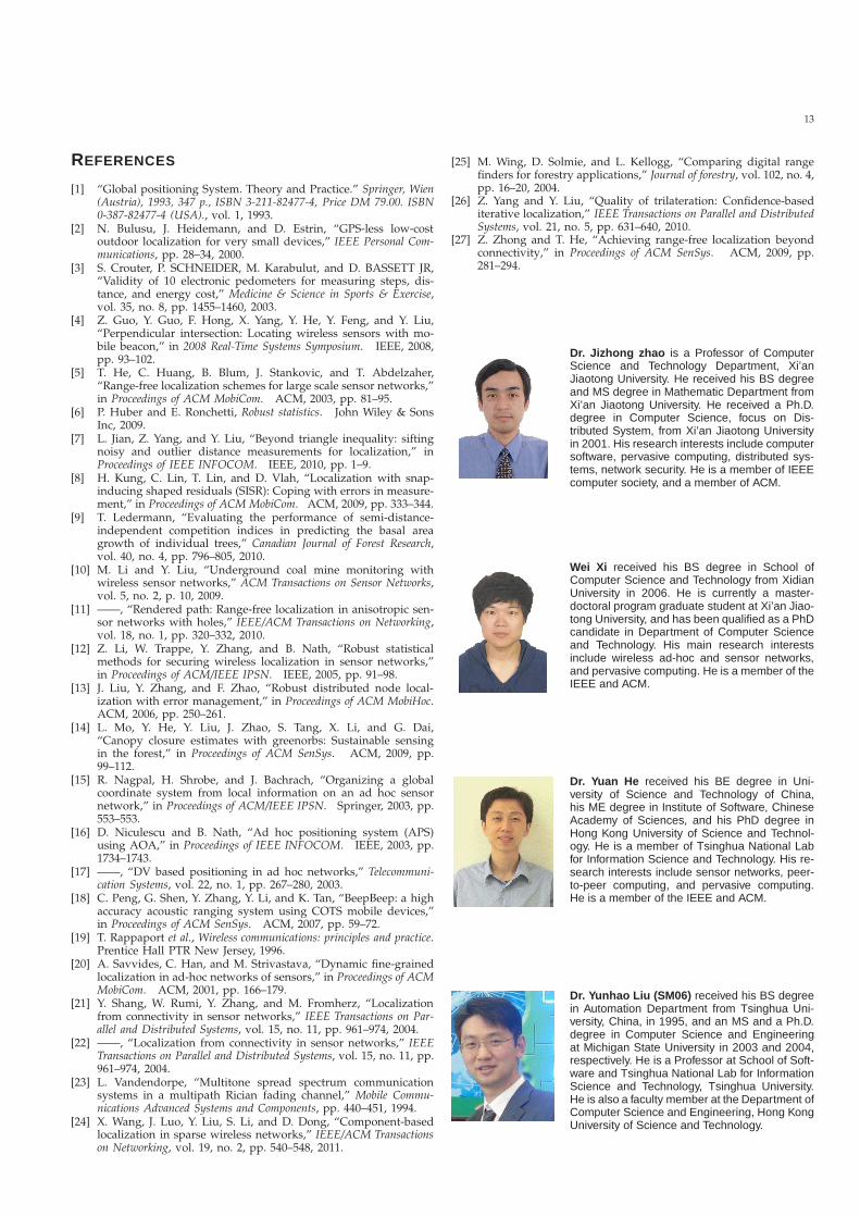
Dr. Jizhong zhao is a Professor of ComputerScience and Technology Department, Xi’anJiaotong University. He received his BS degreeand MS degree in Mathematic Department fromXi’an Jiaotong University. He received a Ph.D.degree in Computer Science, focus on Dis-tributed System, from Xi’an Jiaotong Universityin 2001. His research interests include computersoftware, pervasive computing, distributed sys-tems, network security. He is a member of IEEEcomputer society, and a member of ACM.

Wei Xi received his BS degree in School ofComputer Science and Technology from XidianUniversity in 2006. He is currently a master-doctoral program graduate student at Xi’an Jiao-tong University, and has been qualified as a PhDcandidate in Department of Computer Scienceand Technology. His main research interestsinclude wireless ad-hoc and sensor networks,and pervasive computing. He is a member of theIEEE and ACM.

Dr. Yuan He received his BE degree in Uni-versity of Science and Technology of China,his ME degree in Institute of Software, ChineseAcademy of Sciences, and his PhD degree inHong Kong University of Science and Technol-ogy. He is a member of Tsinghua National Labfor Information Science and Technology. His re-search interests include sensor networks, peer-to-peer computing, and pervasive computing.He is a member of the IEEE and ACM.

Dr. Yunhao Liu (SM06) received his BS degreein Automation Department from Tsinghua Uni-versity, China, in 1995, and an MS and a Ph.D.degree in Computer Science and Engineeringat Michigan State University in 2003 and 2004,respectively. He is a Professor at School of Soft-ware and Tsinghua National Lab for InformationScience and Technology, Tsinghua University.He is also a faculty member at the Department ofComputer Science and Engineering, Hong KongUniversity of Science and Technology.

14

Dr. Xiang-Yang Li (M’99, SM’08) has been anAssociate Professor (since 2006) and AssistantProfessor (from 2000 to 2006) of Computer Sci-ence at the Illinois Institute of Technology. He re-ceived MS (1999) and PhD (2000) degree at De-partment of Computer Science from Universityof Illinois at Urbana-Champaign. He receivedthe Bachelor degree at Department of ComputerScience and Bachelor degree at Department ofBusiness Management from Tsinghua Univer-sity, China, both in 1995.

Lufeng Mo received his BE degree in Xi’an Jiao-tong University, his ME degree in Pecking Uni-versity. Mo Lufeng is currently working towardsthe Ph.D degree in the Department of ComputerScience and Technology of Xi’an Jiaotong Uni-versity. His research interests include wirelesssensor networks and pervasive computing.

Dr. Zheng Yang (S’06) received his BS degreeat Tsinghua University, China, in 2006 and aPh.D degree in computer science at Hong KongUniversity of Science and Technology. He is cur-rently a postdoc at the Tsinghua National Lab-oratory for Information Science and Technologyand School of Software, Tsinghua University. Hismain research interests include wireless ad-hocand sensor networks, and pervasive computing.He is a member of the IEEE and ACM.