Localization in wireless sensor ad-hoc networks

Xiaobo Long

ECSE 6962 course presentation

What is localization Determine node locations in ad-hoc sensor networks

Distributed Without relying on external infrastructure

Without base stations, satellites, etc. GPS: too expensive

not suitable for low-cost, ad-hoc sensor networks

Why need localization Routing techniques require knowledge of location Sensing tasks require knowledge of location

Introduction

Algorithms requirements

Truly distributed employed on large-scale ad-hoc sensor networks

Self-organizing do not depend on global infrastructure

Robust be tolerant to node failures and range errors

Energy efficient require little computation and communication

Assumptions

Nodes are randomly distributed 2-D environment Static network

Nodes don’t move Anchor nodes

Have a priori knowledge of their own position with respect to some global coordinate system

Important parameters

Range errors describe accuracy of the distance measurements effect accuracy of localization algorithms

Connectivity of the nodes i.e., the average number of neighbors

Anchor fraction some anchor nodes have a priori knowledge of their

own position

Three context parameters are dependent

General algorithms [LR03]-Three phases1. Distance to anchors

• Determine the distances between unknowns and anchor nodes• starting at the anchor nodes, measure distance to neighbors• distance information is flooded into the network• flooding limit• three algorithms

1. Sum-dist2. DV-hop3. Euclidian

2. Node position• Derive for each node a position from its anchor distances

1. Lateration2. Min–max

3. Refinement• Refine the node positions

• using information about the range (distance) to, and positions of, neighboring nodes

Phase1: Distance to anchors Sum-dist

• adding the ranges at each hop during flooding anchors nodes:

send a message identity, position, and a path length set to 0

receiving node: adds the measured range to the path length forwards (broadcasts) the message

if the flood limit allows if the current path length is less than the previous one

result each node have stored the position minimum path length

drawbacks range errors accumulate when distance information is propagated

over multiple hops error is significant for large networks with few anchors and/or poor

ranging hardware

Distance to anchors (cont.) DV-hop

- use topological information instead of summing the (erroneous) ranges.

counting the number of hops calibration: convert hop counts into distances

multiplying the hop count with an average hop distance average hop distance obtained by anchors

drawback fails for highly irregular network topologies where the variance in actual hop distances is very

large

Distance to anchors (cont.) Euclidean

based on the local geometry of the nodes around an anchor anchors: initiate a flood receiver:

receive messages from two neighbors that: know their distance to the anchor know their distance to each other

calculate the distance to the anchor result

two possible distance to anchor solution

neighbor vote: a third neighbor n3 connected to either n1 or n2. replace n1 or n2 with n3

Distance to anchors (cont.)

Phase 2: Node position

Nodes determine their position based on the distance estimates to a number of anchors provided by one of the three Phase 1 alternatives

Sum-dist, DV-hop, or Euclidean

Using: the estimated distances (di) known positions (xi; yi)

Methods Lateration Min–max

Lateration algorithm

(1) unknown position is denoted by (x; y). (2) Linear the system by subtracting the last equation from the first n-1 equations.

(3) Reordering the terms gives a proper system of linear equations in the form Ax = b (4) The system is solved using a standard least-

squares approach:

(6) exceptional cases: the matrix inverse can not be computed and Lateration fails.

* quite expensive in the number of floating point operations that is required.

(5) additional sanity check by computingthe residue between the given distances di and the distances to the location estimate of x

Min–max algorithm

1. For each anchor:• construct a bounding box • using its position & distance

to estimate• [xi-di, yi-di] x [xi+di, yi+di]

2. Determine the intersection of these boxes

• [max(xi-di), max(yi-di)] x

[min(xi+di), min(yi+di)]

3. Position of the node

= center of the intersection box

Phase 3: Refinement― Refine the (initial) node positions computed during phase 2

not all available information used in the first two phases positions are not very accurate, even under good conditions

(high connectivity, small range errors) Iterative refinement procedure

take into account all inter-node ranges nodes update their positions

1. a node broadcasts its position estimate2. receives the positions and range estimates from its neighbors3. performs Lateration procedure of Phase 2 to determine its new position4. refinement stops when position update becomes small -> reports the

final position Problem

errors propagate quickly through the network a single error from 1 node needs only d iterations to affect all nodes

(d: network diameter)

Examples of localization algorithms

Ad-hoc positioning by Niculescu and Nath [NN01] Robust positioning by Savvides, Langendoen and Rabaey [SLR02] N-hop multilateration by Savarese, Park and Srivastava [SPS02]

• compare various alternatives for each phase– simulation on the same platform

• conclusion no single algorithm performs best which algorithm be preferred depends on the conditions

― range errors, connectivity, anchor fraction, etc. still significant room for improving accuracy & increasing coverage

General problems for localization1. insufficient data

lack of absolute reference points or anchors

2. distance measurements are noisy creating additional uncertainty

3. difficult for scalability algorithms that scale linearly with the size of the

network are hard to devise data must be broadcast through wireless

channel limited communications capacity.

Localization with Noisy Range Measurements [MLRT04]

Challenges of network localization with noise• only numerical optimization of distance constraints ---- fails

knowing the length of each graph edge ---- does NOT guarantee a unique realization

• need to handle nodes with ambiguous positions• non-rigid graph

can be continuously deformed to produce an infinite number of different realizations

• rigid graph two kinds of ambiguity

• flip ambiguities• discontinuous flex ambiguities

Can NOT be solved by graph rigidity theory or tests when distance measurements are noisy

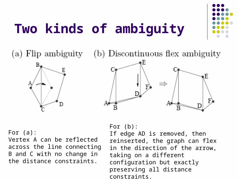
Two kinds of ambiguity

For (a):Vertex A can be reflected across the line connecting B and C with no change in the distance constraints.

For (b):If edge AD is removed, then reinserted, the graph can flex in the direction of the arrow, taking on a different configuration but exactly preserving all distance constraints.

Solution for ambiguity problem

only localize those vertices that: have a small probability of being flip or flex ambiguity

robust quadrilaterals― construct robust quadrilaterals regions to locate node

prevent incorrect realizations of flip ambiguities would otherwise corrupt localization computations

cope with measurement noise in the system drawback

bad performance under low node connectivity

Robust quadrilaterals algorithm Define: cluster

a node and its set of neighbors Three phases

1. Cluster localization Quadrilaterals

the smallest possible sub-graph that can be unambiguously localized in isolation

identify all robust quadrilaterals find the largest sub-graph

• composed solely of overlapping robust quads minimizes the probability of realizing a flip ambiguity

2. Cluster optimization (optional) refine the position estimates for each cluster

using numerical optimization

3. Cluster transformation compute transformations between neighboring clusters

finding the set of nodes in common between two clusters solving for the rotation, translation, and possible reflection that best

aligns the clusters

Quadrilaterals: • knowing the locations of any three vertices

• sufficient to compute the location of the fourth using trilateration• problem

but still NOT sufficient to guarantee a unique graph realization when distance measurements are noisy

If the smallest angle θi is near zero, there is a risk that measurement error

solution restrict our quadrilateral to be robust---> only those triangles with a sufficiently large minimum angle as robust

b is the length of the shortest side and θ is the smallest angle use the robust quadrilateral as a starting point localize additional nodes by chaining together connected robust quads

whenever two quads have three nodes in common & the first quad is fully localized

can localize the second quad by trilaterating from the three known positions

(a) robust four-vertex quadrilateral (b) decomposition of the robust quadrilateral into four triangles.

If θ3 (smallest) is near zero:

say in edge AD, will cause vertex D to be reflected over this sliver of a triangle

Localization with mere connectivity [SRZ03] Goal

using fewer anchor nodes to derive the locations of the nodes even yields relative coordinates when no anchor nodes are available

Method MDS (multi-dimensional scaling)

starts with one or more distance matrices derived from points in a multidimensional space

find a placement of the points in a low-dimensional space usually two or three-dimensional

closely related to PCA (principal component analysis) types of MDS techniques

classical metric MDS, replicated MDS, weighted MDS, etc.

• Classical metric MDS tolerates error gracefully

due to the over-determined nature of the solution it can be performed efficiently on large matrices

a closed-form solution

MDS-MAP algorithm- Based on MDS

First step estimate distance between each possible pair of nodes

use shortest-paths algorithm shortest path distances are used to construct the distance matrix for MDS

Second step apply classical MDS to the distance matrix

core of classical MDS SVD (singular value decomposition)

result of MDS a relative map that gives a location for each node

Third step if given sufficient anchor nodes

transform the relative map to an absolute map based on the absolute positions of anchors

Drawback requires centralized computation

Localization for mobile sensor network [HE04]

Usually mobility make localization more difficult

none of above mechanism consider mobile nodes and anchors

Sequential Monte Carlo localization take advantage of mobility

to improve the accuracy of localization reduce the number of anchors required

based on MCL (Monte Carlo Localization) used for robots localization

Sequential Monte Carlo (SMC)

Key idea estimate the posterior distribution of discrete time dynamic models

Algorithm t: discrete time l(t): position distribution of the node at time t o(t): observations from anchor nodes received between time t-1 and time t p(l(t) | l(t-1)): transition equation

prediction of node’s current position based on previous position p(l(t) | o(t)): observation equation

describes the likelihood of the node being at the location l(t) given the observations

filter impossible positions estimate recursively in time the filtering distribution p(l(t) | o(0), o(1), …, o(t)) A set of N samples L(t) is used to represent the distribution l(t) recursively computes the set of samples at each time step since L(t-1) reflects all previous observations, can compute l(t) using only L(t-

1) and o(t).

Conclusion

Goal determine node locations in ad-hoc sensor

networks can use a small number of anchors

Three phases various alternatives for each phase

Challenges noisy distance measurements mere connectivity mobility

Reference1. Ian F. Akyildiz, Weilian Su, Yogesh Sankarasubramaniam, and Erdal Cayirci, A

Survey on Sensor Networks.2. [LR02] Koen Langendoen, Niels Reijers, Distributed localization in wireless sensor

networks: a quantitative comparison, Computer Networks, 2003, pp. 499-518.3. [NN01] D. Niculescu, B. Nath, Ad-hoc positioning system, IEEE GlobeCom, 2001.4. [SLR02] C. Savarese, K. Langendoen, J. Rabaey, Robust positioning algorithms

for distributed ad-hoc wireless sensor networks, USENIX Technical Annual Conference, 2002, pp. 317–328.

5. [SPS02] A. Savvides, H. Park, M. Srivastava, The bits and flops of the N-hop multilateration primitive for node localization problems, in: First ACM International Workshop on Wireless Sensor Networks and Application (WSNA), 2002, pp. 112–121.

6. [MLRT04] David Moore, John Leonard, Daniela Rus and Seth Teller, Robust Distributed Network Localization with Noisy Range Measurements, ACM, 2004.

7. [SRZ03] Yi Shang, Wheeler Ruml, Ying Zhang, Markus P. J. Fromherz, Localization from Mere Connectivity, MobiHoc, 2003.

8. [HE04] Lingxuan Hu, David Evans, Localization for Mobile Sensor Networks, MobiCom, 2004.