Localisation using an image-map

Chanop Silpa-AnanThe Australian National University

chanop@syseng.anu.edu.au

Richard HartleyNational ict Australia

hartley@syseng.anu.edu.au

Abstract

This paper looks at the problem of building a visualmap for later localisation using images from a typ-ical digital camera. The main objective is an abil-ity to query and match images in general positionagainst a large image data set or an image-map.We have achieved a quick localisation in terms offinding a label of the map by finding similar imagesin the data set. We use affinely invariant Harris cor-ners and sift descriptors to represent 2d images. Akd-tree is used for indexing, matching, and group-ing the data set to form a visual map database. Forthis application, we have improved a voting tech-nique for a 3d structure and a run-time efficiency ofkd-tree to allow a quick finding of similar imagesand a quick localisation. The result can be appliedto a more generic localisation (for mobile robotics)and may be integrated in a visual odometry system.

1 Introduction

Machine vision has gained more acceptance in the roboticscommunity. Humans use visual information extensively in ev-eryday life. Replicating a human vision in a machine visionis an appealing challenge. In this paper, we are looking at theproblem of using 3d vision for map building and localisation.

Remembering places where one has been before and read-ing maps are (quite) easy tasks for humans. On the contrary,it is fairly difficult to replicate these behaviour in machines tothe level that humans can do. The map problem is one of thefundamental tasks in mobile robotics. In this field, there aretwo popular approaches to implement a map: a metric mapand a topological map.

In its simplest form, given a map and observations, localisa-tion is matching observations to the map. For a visual map Inthe past, visual features or visual landmarks have been usedin conjunction with other types of sensors to build the map.There have been some attempts to use only visual information;hence, locating and matching visual features become the mainchallenge. It is also a requirement for localisation purposes to

match visual features in an observed image with those in themap.

Map from imagesWe envision a map created purely from images to be usefulfor: 1. finding if we are on the map, given an observation im-age; and 2. finding where we are on the map. With one objec-tive of using a visual map for navigation and localisation, wethink of the map created from images as follows. Suppose weare making a floor-plan-like map of an indoor office environ-ment by taking a lot of images of the scene. Creating a simplemap is laying down these images on a paper (according totheir locations) and make links between these images if theymatch. According to the subject of multiple view geometry,we may, with more effort, reconstruct the scene and make a3d map.

In this paper, we use sift descriptors [Lowe, 1999] com-puted at detected Harris-affine interest points [Mikolajczykand Schmid, 2002] to represent images. We demonstrate animproved indexing technique with a kd-tree optimised for siftdescriptors, an improved voting technique for finding candi-date location in a map, and an improved ransac geared forapplications that have a large fraction of outliers. With theseimprovements, visual localisation is more plausible in real ap-plication.

An image-map in our term is a correspondence graph witheach image being a vertex in the graph. Similar images takenfrom the same location are linked by graph edges; hence, theyform a clique in the graph. Each image node may be labelledby its corresponding 3d position in the real world, and thenwe can use this image-map for the real world localisation. Thelinks between images are usually stitched together by imagetracking and image matching techniques. We enhance the us-age of this map representation – at the moment, for voting – inthat we encode overlapped regions between two images intothe edge property so that we can use this geometric informa-tion to help score votes. When a match point from a query im-age lies in these overlapped regions in either image, the voteis propagated to the other image.

In more details, our procedures for building a visual mapare:

1. Given a set of images, extract interest points andcompute a descriptor for each point.

2. Match these images with their interest points anddescriptors.

3. Verify these matches with 2d/3d constraints.

4. Label the matched points and the matched images.

5. Reconstruct the 3d points and camera positions frommatched points if building a metric map.

For localisation, we match an image with those in the map tofind out quickly where the image is in relation to the map. Theprocedures are:

1. Given a query image, extract interest points andcompute a descriptor for each point.

2. Match the image (with its interest points anddescriptors) with those in the map database.

3. Verify these matches with 2d/3d constraints.

4. For a metric map, compute the camera position frommatched points.

2 A set of visual features approachFinding correspondences between images is a fundamentalproblem for building geometric relationships. There are manytypes of image correspondences. A large number of applica-tions use short baseline stereo techniques which mainly as-sume that two images are fairly similar. In a wide baselinestereo, two images differ more significantly; hence, findingcorrespondences becomes more difficult and requires a differ-ent set of techniques.

For map building, we may take many images to form adense data set. However, a dense data set implies a large stor-age space and a search though a large data set. Wide baselinestereo techniques allow a sparser data set and images are ex-pected to be significantly different in terms of scale, orienta-tion, and perspective.

Recently, matching images with interest points and imagedescriptors has shown a promising capability to match im-ages taken from quite different view points [Brown and Lowe,2002; Dufournaud et al., 2000; Schafalitzky and Zisserman,2002]. Moreover, the same technique has been adapted for2d image retrieval from a large database [Schmid and Mohr,1997] and object recognition [Lowe, 1999]. Along the line ofvisual maps, there was an attempt to use this technique formobile robot localisation and map building [Se et al., 2002].

A multi-scale interest point detector (a multi-scale frame-work) has been developed in [Lindeberg, 1994; 1998a; 1998b]using a Hessian matrix based interest point detector, for ex-ample: a Laplacian of Gaussian. In [Schmid et al., 2000],many interest point detectors were studied and compared, anda multi-scale Harris detector was suggested as the best per-former. Later on, an improved version, a Harris-affine was pro-posed as an affinely invariant interest point detector [Mikola-jczyk and Schmid, 2002]. The Harris-affine detector was used

to compare several local image descriptors in [Mikolajczykand Schmid, 2003]. As a result, a sift descriptor citelowe:99was suggested based on its performance. Other well perform-ing descriptors were steerable filters [Freeman and Adelsan,1991], complex filters [Schafalitzky and Zisserman, 2002],and moment invariants [Tuytelaars and Gool, 2000].

3 Correspondence problem

Finding correspondences between images is basically theheart of the visual aspect of map building and localisation.There are two main types of image matching in this problem.The first one is matching a query image against the map forlocalisation, and the second one is matching between a set ofimages for map building. In one perspective, if we take an ap-proach of building a map by adding one image at time to themap, finding correspondences between the new image and ex-isting images is similar to finding correspondences betweenthe query image and the map. Matching the query image withthe set of images is a two step process. Firstly, we match de-scriptors in the query image with those in the data set. Thensecondly, we infer from a set of matched descriptors for cor-responding (matched) images.

An image descriptor is represented as a real vector in a fixedhigh dimensional space, d ∈ Rd . Finding a match or matchesof a query vector dq among a set of descriptors in a database{di } is a nearest-neighbour problem. In high dimensions, thisproblem is difficult to deal with. In some circumstances, thebest result is from a linear search. For map building and lo-calisation, we may assume that a map is static once it is built,or it is modified infrequently. We may also assume that it isbeing used (queried) a lot more often than being modified.The best approach in order to localise quickly is to create adata structure such that nearest-neighbour queries can be an-swered quickly. A kd-tree [Bentley, 1975; Freidman et al.,1977] is one suitable data structure which allows a nearest-neighbour search in high dimensional space. It has been usedpreviously to index image descriptors [Beis and Lowe, 1997;Schmid and Mohr, 1997].

An improved KD-tree

We use a kd-tree data structure for indexing a set of descrip-tors {di } that are part of the map. The kd-tree allows a nearest-neighbour query in the form of finding a vector di that is clos-est to a query vector dq by a metric norm

∥∥dq − di

∥∥. Even

though the kd-tree was designed for high dimensional dataand was originally claimed to have logarithm search timeO(log n) [Freidman et al., 1977], in many cases, it does notoutperform a linear search O(n) by a large margin. Some con-ditions that the kd-tree performs close to the theoretical anal-ysis were suggested in the original paper.

The kd-tree has been adapted for approximate nearestneighbour search [Beis and Lowe, 1997; Arya et al., 1998]; byrelaxing the goal to search for an approximate nearest match,

0

0.1

0.2

0.3

0.4

0.5

0 100 200 300 400 500 600 700 800 900 1000

Pr(e

)

Maximum number of search nodes

kd-tree’s and nkd-tree’s error

kd-treenkd-tree

Figure 1: [An improved kd-tree] The above figure illustratesan improvement of our kd-tree search algorithm over astandard priority search. The graph shows errors in gettingwrong nearest neighbour answers. By employing multiplekd-tree and pca, we improved the probability of gettingcorrect answer under the same condition of maximumnumber of search nodes. The data set was 500 000 siftfeatures of 128 dimensions computed from 600 images. Thequeries were 5 000 sift features taken from the same dataset and corrupted with Gaussian noises in every dimension.

its performance can be improved vastly. Independently devel-oped in both papers, an algorithm priority search can find thetrue nearest neighbour with high probability. The algorithmsearches the kd-tree by ranking search nodes by their distancefrom the query point. Under a constant search time constraint,in applications that require a fixed run-time for example, thepriority search finds the true nearest neighbour most of thetime, and for the rest, it finds a close approximation.

The sift descriptor, as suggested in [Beis and Lowe, 1997],has 128 dimensions. The kd-tree, which is an extension to abinary tree, requires approximately at least 3 × 1038 points(2128 points) in order to have splitting nodes covering everydimension. Using the kd-tree with 128 dimensional descrip-tors for a much small number of points, for practical reasons,means that many dimensions are not covered by the tree. Forexample, one million points (in double floating point preci-sion, this requires one gigabyte of ram) cover maximally 20dimensions (log2 106 dimensions); therefore, 108 dimensionsare not constrained by the tree.

In a work described in more detail in a separate paper,we further improved the kd-tree’s search performance aimedspecifically for searching sift descriptors and also other typesof local image descriptor in high dimensions. We used twomain techniques: employing multiple kd-trees of the samedata set to extend the dimensions covered by kd-tree and ex-ploiting the internal structure of descriptor through the princi-pal component analysis (pca). In the context of matching siftfeatures, the pca reveals that the number of components thathave eigenvalues within 10% of the maximum eigenvalue is

much less than 128. We found that the number of importantdimensions, using 10% criterian, is approximately 35 dimen-sions. The pca reduces the complexity in dimensions at theexpense of projecting points into a lower dimensional space.

As a result of using multiple search trees and exploiting theprincipal components, we improve the kd-tree’s ability to findthe true nearest neighbour under a constant run-time (fixednumber of search nodes) over that of a standard priority searchalgorithm. This property makes the usage of visual maps moreplausible in real (real-time) applications.

Consensus locationA kd-tree allows us to match a query descriptor against everydescriptors stored in the map directly. This has a particularadvantage in that it implies a search for matched images. In[Schmid and Mohr, 1997], a voting mechanism was used tofind images from a large data set that are similar to the queryimage. The largest consensus is the most probable answer. Thebasis is similar to that of the Hough transform: each matcheddescriptor votes for its associated image. There are a numberof constraints which may be easily used in conjunction withstraight voting:

• [One match] Each descriptor may vote for only one de-scriptor in each image; however, it may vote for severaldescriptors in different images.

• [Neighbourhood match] Each descriptor can vote for animage if there are nearby descriptors that vote for thesame image.

• [Weak local geometry] Each descriptor can vote for animage if there are nearby descriptors that vote for thesame image with similar geometry: scale, orientation,and distance.

In voting, each descriptor may vote for the best matched de-scriptor or each descriptor may vote for several best matcheddescriptors. Voting for several best matched descriptors re-quires either a fixed number of votes or a fixed thresholdlevel where

∥∥dq − di

∥∥ is acceptable. Both ways tend to lead

to many false matches when geometric constraints are not ap-plied. Therefore we incline to vote for the best match only.

Voting for the best match has its own problem: we foundedthat voting for one best match tends to dilute voting scoreswhen there are several images that are very similar in the dataset. Voting for one best match means that only one of theseimages gets the vote.

Because we have an objective of creating a visual map forlocalisation, we would like to use implicit knowledge of themap to help voting. Suppose we have a 3d euclidean map withpoint Xi and its set of descriptors {d j

i }; each descriptor d ji is

a descriptor of 2d point xi in image I j . Ultimately, we wouldlike to match the query point xq and 3d points in the map. Itis difficult to match directly because of the size of the data set;nevertheless, voting helps to achieve this goal by pruning outimpossibilities. We string descriptors of point xi in image I j

q

x

C ′

C

x′

X

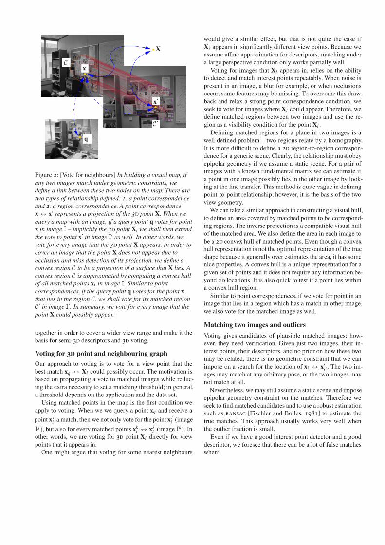
Figure 2: [Vote for neighbours] In building a visual map, ifany two images match under geometric constraints, wedefine a link between these two nodes on the map. There aretwo types of relationship defined: 1. a point correspondenceand 2. a region correspondence. A point correspondencex ↔ x′ represents a projection of the 3d point X. When wequery a map with an image, if a query point q votes for pointx in image I – implicitly the 3d point X, we shall then extendthe vote to point x′ in image I′ as well. In other words, wevote for every image that the 3d point X appears. In order tocover an image that the point X does not appear due toocclusion and miss detection of its projection, we define aconvex region C to be a projection of a surface that X lies. Aconvex region C is approximated by computing a convex hullof all matched points xi in image I. Similar to pointcorrespondences, if the query point q votes for the point xthat lies in the region C, we shall vote for its matched regionC ′ in image I′. In summary, we vote for every image that thepoint X could possibly appear.

together in order to cover a wider view range and make it thebasis for semi-3d descriptors and 3d voting.

Voting for 3D point and neighbouring graphOur approach to voting is to vote for a view point that thebest match xq ↔ Xi could possibly occur. The motivation isbased on propagating a vote to matched images while reduc-ing the extra necessity to set a matching threshold; in general,a threshold depends on the application and the data set.

Using matched points in the map is the first condition weapply to voting. When we we query a point xq and receive a

point x ji a match, then we not only vote for the point x j

i (image

I j ), but also for every matched points xki ↔ x j

i (image Ik). Inother words, we are voting for 3d point Xi directly for viewpoints that it appears in.

One might argue that voting for some nearest neighbours

would give a similar effect, but that is not quite the case ifXi appears in significantly different view points. Because weassume affine approximation for descriptors, matching undera large perspective condition only works partially well.

Voting for images that Xi appears in, relies on the abilityto detect and match interest points repeatably. When noise ispresent in an image, a blur for example, or when occlusionsoccur, some features may be missing. To overcome this draw-back and relax a strong point correspondence condition, weseek to vote for images where Xi could appear. Therefore, wedefine matched regions between two images and use the re-gion as a visibility condition for the point Xi .

Defining matched regions for a plane in two images is awell defined problem – two regions relate by a homography.It is more difficult to define a 2d region-to-region correspon-dence for a generic scene. Clearly, the relationship must obeyepipolar geometry if we assume a static scene. For a pair ofimages with a known fundamental matrix we can estimate ifa point in one image possibly lies in the other image by look-ing at the line transfer. This method is quite vague in definingpoint-to-point relationship; however, it is the basis of the twoview geometry.

We can take a similar approach to constructing a visual hull,to define an area covered by matched points to be correspond-ing regions. The inverse projection is a compatible visual hullof the matched area. We also define the area in each image tobe a 2d convex hull of matched points. Even though a convexhull representation is not the optimal representation of the trueshape because it generally over estimates the area, it has somenice properties. A convex hull is a unique representation for agiven set of points and it does not require any information be-yond 2d locations. It is also quick to test if a point lies withina convex hull region.

Similar to point correspondences, if we vote for point in animage that lies in a region which has a match in other image,we also vote for the matched image as well.

Matching two images and outliers

Voting gives candidates of plausible matched images; how-ever, they need verification. Given just two images, their in-terest points, their descriptors, and no prior on how these twomay be related, there is no geometric constraint that we canimpose on a search for the location of xi ↔ x′

i ′ . The two im-ages may match at any arbitrary pose, or the two images maynot match at all.

Nevertheless, we may still assume a static scene and imposeepipolar geometry constraint on the matches. Therefore weseek to find matched candidates and to use a robust estimationsuch as ransac [Fischler and Bolles, 1981] to estimate thetrue matches. This approach usually works very well whenthe outlier fraction is small.

Even if we have a good interest point detector and a gooddescriptor, we foresee that there can be a lot of false matcheswhen:

Figure 3: [Typical matching] This figure illustrates a typicalmatching result of two images with their interest points anddescriptors. For these results we use Harris-affine interestpoint detector and sift descriptors in 128 dimensions. Inthese images, we show the matched regions by their convexhull representation and matched interest points by their 2dDelaunay triangulated mesh – for visualisation purpose only.Non-matched interest points are shown in plain green dots.We use ransac algorithm to estimate inliers and outliersfrom match candidates with constant on fundamental matrix;inlier fraction was 0.156 (197/1256) which requires1.28 × 106 iterations for a standard ransac to guaranteeconfidence level of 0.95. For this pair of images, we limitedour improved ransac to 2 000 iterations.

• Two images match partially, either from a scale differ-ence, or from different view angle;

• Two images do not match;

• There are a significant number of similar objects.

Trying to find matched candidates for every point in the twoimages would lead to a lot of outliers. A threshold on descrip-tor match,

∥∥dq − di

∥∥, may be imposed, but it does not guar-

antee to compensate for all the false matches.A ransac type algorithm is still applicable, but its run-

time grows quickly as the outlier fraction increases. In anotherwork described in more details in a separate paper, we improve

Figure 4: [Small overlapped region]When two images havesmall overlapped region, outlier fraction is large. This figureillustrates when we find two matched images with smalloverlapped region. The detected matched region is evensmaller than the actual overlapped area. Inlier fraction is0.063 (19/300) which requires 7.33 × 108 for a confidencelevel of 0.95; we also limit our improved ransac to 2 000iterations for this pair of images.

ransac for an application where the outlier fraction is large.Basically, we use the descriptor matching score,

∥∥dq − di

∥∥,

to guide the hypothesis generation by using more of the bettermatches. We also reduced ransac’s run-time by early discard-ing bad hypotheses.

Loop-back detection

One major problem in map building is being able to detectwhether we have travelled back to the same place. Data associ-ation is typically difficult and expensive in a global framework.With the previously described techniques, we can quickly findif similar images have been encountered before and loop-backdetection is a by-product that we can use to further constrain3d reconstruction.

4 ResultsTo illustrate the application of this technique in visual mapbuilding, we use a data set of office images. The data set con-

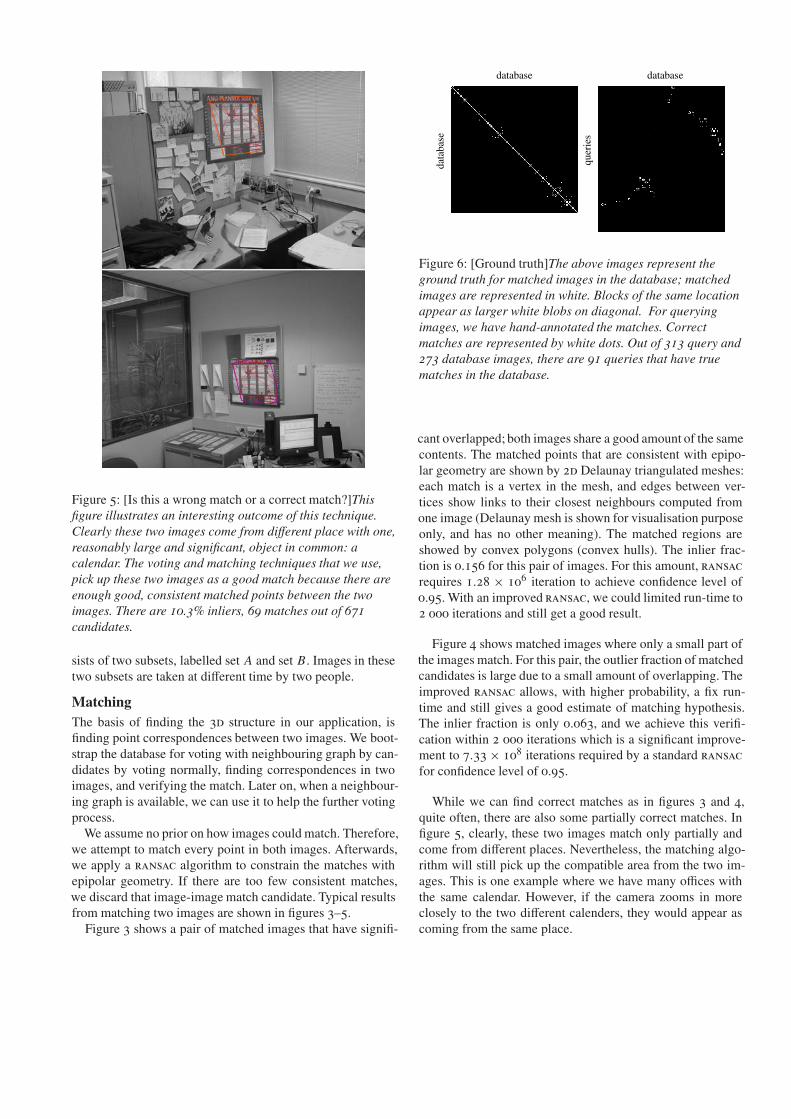
Figure 5: [Is this a wrong match or a correct match?]Thisfigure illustrates an interesting outcome of this technique.Clearly these two images come from different place with one,reasonably large and significant, object in common: acalendar. The voting and matching techniques that we use,pick up these two images as a good match because there areenough good, consistent matched points between the twoimages. There are 10.3% inliers, 69 matches out of 671candidates.

sists of two subsets, labelled set A and set B . Images in thesetwo subsets are taken at different time by two people.

MatchingThe basis of finding the 3d structure in our application, isfinding point correspondences between two images. We boot-strap the database for voting with neighbouring graph by can-didates by voting normally, finding correspondences in twoimages, and verifying the match. Later on, when a neighbour-ing graph is available, we can use it to help the further votingprocess.

We assume no prior on how images could match. Therefore,we attempt to match every point in both images. Afterwards,we apply a ransac algorithm to constrain the matches withepipolar geometry. If there are too few consistent matches,we discard that image-image match candidate. Typical resultsfrom matching two images are shown in figures 3–5.

Figure 3 shows a pair of matched images that have signifi-

quer

ies

database database

data

base

Figure 6: [Ground truth]The above images represent theground truth for matched images in the database; matchedimages are represented in white. Blocks of the same locationappear as larger white blobs on diagonal. For queryingimages, we have hand-annotated the matches. Correctmatches are represented by white dots. Out of 313 query and273 database images, there are 91 queries that have truematches in the database.

cant overlapped; both images share a good amount of the samecontents. The matched points that are consistent with epipo-lar geometry are shown by 2d Delaunay triangulated meshes:each match is a vertex in the mesh, and edges between ver-tices show links to their closest neighbours computed fromone image (Delaunay mesh is shown for visualisation purposeonly, and has no other meaning). The matched regions areshowed by convex polygons (convex hulls). The inlier frac-tion is 0.156 for this pair of images. For this amount, ransacrequires 1.28 × 106 iteration to achieve confidence level of0.95. With an improved ransac, we could limited run-time to2 000 iterations and still get a good result.

Figure 4 shows matched images where only a small part ofthe images match. For this pair, the outlier fraction of matchedcandidates is large due to a small amount of overlapping. Theimproved ransac allows, with higher probability, a fix run-time and still gives a good estimate of matching hypothesis.The inlier fraction is only 0.063, and we achieve this verifi-cation within 2 000 iterations which is a significant improve-ment to 7.33 × 108 iterations required by a standard ransacfor confidence level of 0.95.

While we can find correct matches as in figures 3 and 4,quite often, there are also some partially correct matches. Infigure 5, clearly, these two images match only partially andcome from different places. Nevertheless, the matching algo-rithm will still pick up the compatible area from the two im-ages. This is one example where we have many offices withthe same calendar. However, if the camera zooms in moreclosely to the two different calenders, they would appear ascoming from the same place.

20

40

60

80

100

120

140

1 2 3 4 5 6 7 8 9 1011121314151617181920

Num

ber

ofvo

tes

Rankings

Voting – one image

Match - new votingCandidate - new voting

Match - votingCandidate - voting

100

150

200

250

1 2 3 4 5 6 7 8 9 10

No.

ofto

talc

orre

ctan

swer

s

Number of examined candidates per query

Voting - corect answers

new votingvoting

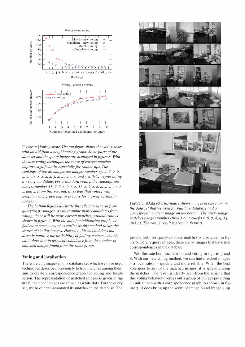
Figure 7: [Voting score]The top figure shows the voting scorewith an aid from a neighbouring graph. Some parts of thedata set and the query image are displayed in figure 8. Withthe new voting technique, the score of correct matchesimprove significantly, especially for runner-ups. Therankings of top 20 images are images number 15, 7, 8, 9, 6,x, x, x, x, x, x, x, x, 3, x, x , x, x, x, and x with ‘x’ representinga wrong candidate. For a standard voting, the rankings areimages number 15, 7, 8, x, 9, x, x, 13, x, 6, x, x, x, x, x, x, x, x,x, and x. From this scoring, it is clear that voting withneighbouring graph improves score for a group of similarimages.

The bottom figures illustrate this effect in general fromquerying 91 images. As we examine more candidates fromvoting, there will be more correct matches; ground truth isshown in figure 6. With the aid of neighbouring graph, wefind more correct matches earlier as this method raises thescores of similar images. However, this method does notdirectly improve the probability of finding a correct match,but it does hint in terms of confidence from the number ofmatched images found from the same group.

Voting and localisationThere are 273 images in this database set which we have usedtechniques described previously to find matches among themand to create a correspondence graph for voting and locali-sation. The representation of matched images is given in fig-ure 6; matched images are shown as white dots. For the queryset, we have hand-annotated its matches in the database. The

Figure 8: [Data set]This figure shows images of one room inthe data set that we used for building database and acorresponding query image on the bottom. The query imagematches images number (from 1 on top-left) 3, 6, 7, 8, 9, 13,and 15. The voting result is given in figure 7.

ground truth for query-database matches is also given in fig-ure 6. Of 313 query images, there are 91 images that have truecorrespondences in the database.

We illustrate both localisation and voting in figures 7 and8. With our new voting method, we can find matched images– a localisation – quickly and more reliably. When the bestvote goes to any of the matched images, it is spread amongthe matches. The result is clearly seen from the scoring thatthis voting behaviour brings out a group of images providingan initial map with a correspondence graph. As shown in fig-ure 7, it does bring up the score of image 6 and image 9 up

to the top. Voting with neighbouring graph yields more cor-rect matches among the top candidates. Because images inthe map database are matched and labelled, we can infer withgreater confidence about the localisation of the query imagewhen many images of the same label come up frequently.

The other benefit of this method in incrementally building amap – not shown in this paper – is that we can go through thelist of matched candidates and verify the match one by one;with a more reliable ranking, we would are verifying moretrue matches before encountering a false one.

5 ConclusionWe have demonstrated our strategy of creating a visual mapfor quick localisation. In making the visual map more plau-sible for real application, we have shown that: an improvetechnique for kd-tree indexing allows a greater possibility ina fixed-time search; a 3d voting allows a direct inferring ofcamera localisation with respected to labelled places in a map;and an improved ransac which allows a good hypotheses es-timation, in the presence of large outlier fraction, in a shorterrun-time. This work can also be extended to a full 3d recon-struction of a visual map which would have more applicationsin metric localisatioa and it may also be integrated into a fullvisual odometry system.

AcknowledgementLastly, we thank David Lowe for giving his sift descriptorcode for our studying, Krystian Mikolajczyk for providing aHarris-affine detector program from his web page, TargetJrand vxl projects for providing many useful tools, and BillTriggs for insightful discussions.

References[Arya et al., 1996] Sunil Arya, David M. Mount, and Onuttom

Narayan. Accounting for boundary effects in nearest neighborsearching. Discrete and computational geometry, 16:155–176,1996.

[Arya et al., 1998] Sunil Arya, David M. Mount, Nathan S.Netanyahu, Ruth Silverman, and Angela Y. Wu. An optimalalgorithm for approximate nearest neighbor searching in fixeddimensions. Journal of the acm, 45(6):891–923, 1998.

[Beis and Lowe, 1997] Jeffrey S. Beis and David G. Lowe. Shapeindexing using approximate nearest–neighbour search inhigh–dimensional spaces. In Proceedings of computer visionand pattern recognition, pages 1000–1006, Puerto Rico, June1997.

[Bentley, 1975] Jon Louis Bentley. Multidimensional binarysearch trees used for associative searching. Communications ofthe acm, 18(9):509–517, 1975.

[Brown and Lowe, 2002] Mathew Brown and David Lowe.Invariant features from interest point groups. In Proceedings ofBritish machine vision conference, pages 656–665, Cardiff,Wales, September 2002.

[Dufournaud et al., 2000] Yves Dufournaud, Cordelia Schmid, andRadu Horaud. Matching images with different resolutions. In

Proceedings of computer vision and pattern recognition,volume 1, pages 612–618, June 2000.

[Fischler and Bolles, 1981] Martin A. Fischler and Robert C.Bolles. Random sample consensus: A paradigm for modelfitting with applications to image analysis and automatedcartography. Computer vision, graphics and image processing,24(6):381–395, 1981.

[Freeman and Adelsan, 1991] Willaim T. Freeman and Edward H.Adelsan. The design and use of steerable filters. ieeetransaction on pattern analysis and machine intelligence,13(9):981–906, September 1991.

[Freidman et al., 1977] Jerome H. Freidman, Jon Louis Bently,and Raphael Arifinkel. An algorithm for finding best matches inlogarithmic expected time. acm transactions on mathematicalsoftware, 3(3):209–206, september 1977.

[Lindeberg, 1994] Tony Lindeberg. Scale-space theory: a basictool for analysing structures at different scales. Journal ofapplied statistics, 21(2):224–270, 1994.

[Lindeberg, 1998a] Tony Lindeberg. Feature detection withautomatic scale selection. International journal of computervision, 30(2):77–116, 1998.

[Lindeberg, 1998b] Tony Lindeberg. Principles for automatic scaleselection. Technical Report isrn kth textscna/p–98/14–se, kth(Royal Institute of Technology), 1998.

[Lowe, 1999] David G. Lowe. Object recognition from localscale–invariant features. In Proceedings of internationalconference on computer vision, pages 1150–1157, Greece,September 1999.

[Mikolajczyk and Schmid, 2002] Krystian Mikolajczyk andCordelia Schmid. An affine invariant interest point detector. InProceedings of the European conference on computer vision,volume 1, pages 128–142, Denmark, 2002.

[Mikolajczyk and Schmid, 2003] Krystian Mikolajczyk andCordelia Schmid. A performance evaluation of local descriptors.In Proceedings of computer vision and pattern recognition,2003.

[Schafalitzky and Zisserman, 2002] Frederik Schafalitzky andAndrew Zisserman. Multi-view matching for unordered imagesets, or ‘How do I organize my holiday snaps?’. In Proceedingsof the European conference on computer vision, Denmark, 2002.

[Schmid and Mohr, 1997] Cordelia Schmid and Roger Mohr.Local greyvalue invariants for image retrieval. ieee transactionon pattern analysis and machine intelligence, 1997.

[Schmid et al., 2000] Cordelia Schmid, Roger Mohr, and ChristianBauckhage. Comparing and evaluating interest points.International journal of computer vision, 37(2):151–172, 2000.

[Se et al., 2002] Stephen Se, David Lowe, and Jim Little. Mobilerobot localization and mapping with uncertainty usingscale–invariant visual landmarks. International journal ofrobotics research, 21(8):735–758, August 2002.

[Tuytelaars and Gool, 2000] Tinne Tuytelaars and Luc Van Gool.Wide baseline stereo matching based on local, affinely invariantregions. In Proceeding of British machine vision conference,pages 412–425, Bristol, United Kingdom, 2000.