local oscillator phase noise effects - inside gnssinsidegnss.com/auto/novdec10-thombre.pdf ·...

52 InsideGNSS n o v e m b e r / d e c e m b e r 2 0 1 0 www.insidegnss.com

GNSS systems rely on direct sequence spread spectrum (DSSS) transmissions to achieve high receiver sensitivity. Typi-

cally, GNSS user equipment compares the signal received from a satellite with an internally generated replica of its cor-responding code until the maximum

correlation for a given delay is achieved. This provides an indirect measurement of the satellite-receiver range.

One of the performance limiting fac-tors of GNSS receivers is the imperfec-tion of the radio frequency (RF) oscil-lator. This imperfection translates into random deviations of instantaneous phase or frequency, typically modeled as a phase imperfection, and often referred to as phase noise.

The receiver oscillator phase noise narrows the carrier tracking loop band-width, while diminishing the achievable carrier-to-noise ratio (C/N0). The corre-lation outputs in the code-tracking loop are also affected, creating correlation noise and losses at the receiver that are measured as reductions in C/N0.

Furthermore, longer integration intervals ideally result in higher sensi-tivity. However, because phase noise is translated into a rotation of the constel-lation diagram of a modulated signal that can make integration (correlation) comparatively less effective as the inter-val increases.

Phase noise models have been pro-posed for various wireless communica-tion receivers. (See the sidebar, “Mod-eling Phase Noise Effects on Receivers: A History” on page 54.) However, the effects of phase noise on GNSS receiv-ers’ performance have been rarely doc-umented, leaving key design questions unanswered: What is the maximum acceptable phase noise level as required by an RF designer in order to achieve a

Local oscillator Phase noise effects on GnSS code Tracking

A new perspective for GNSS designers quantifies the performance loss due to phase noise effects on the baseband signal. These performance bounds may then be used as the basis for local oscillator design. The authors develop bounds by identifying front-end local oscillator phase noise effects on the correlation loss, while tracking receiver performance. Until now, this effect has been rarely documented in research literature. Extensive simulations are used to validate results, while drawing conclusions regarding the relationship between phase noise, correlation time, and loss in the carrier-to-noise ratio.

© iS

tock

phot

o.co

m/E

ugen

e Ka

zim

iaro

vich

erneSTo Pérez Serna, Acorde Technologies s.A

SaranG Thombre, mikko vaLkama, Simona Lohan, viLLe SyrjäLäTAmpere UniversiTy of Technology

marco deTraTTiAcorde Technologies s.A

heikki hurSkainen, jari nurmiTAmpere UniversiTy of Technology

www.insidegnss.com n o v e m b e r / d e c e m b e r 2 0 1 0 InsideGNSS 53

minimum pre-defined C/N0? How do correlation losses relate to phase noise levels?

In this article, we propose an analytical approach using a given phase noise model, validating it through simulations to quantify the effect of oscillator noise on the performance of GNSS receivers. From this we provide a first estimation of the requirements of a radio front-end for a given baseband imple-mentation, as well as an insight into the relationship between correlation time and performance degradation due to phase noise. The following section of our discussion provides a theo-retical analysis, in both time-domain and frequency-domain, of the effect of this phase noise on various properties of code correlation.

We then perform numerical simulations of GPS L1 pseu-dorandom noise (PRN) code correlation for various values of phase noise in order to validate the theoretical model. Next, a datastream simulation using a Galileo E1 receiver, complete with carrier and code tracking loops, quantifies the effect of oscillator noise on GNSS receiver performance. Here, the simulated PRN code correlation in the presence of phase noise demonstrates that the model (and GPS results) may be applied to Galileo signal receivers as well.

Finally, we compare results from all the simulations and recommend a practical limit for the maximum phase noise permissible from the front-end oscillator in order to maintain the post-correlation signal-to-noise ratio (SNR) of a correlation peak beneath a given threshold.

Our results provide a first estimate of the noise floor require-ments for a receiver given a particular baseband implemen-tation. Also, this study provides insight into the relationship between correlation time and performance degradation due to phase noise.

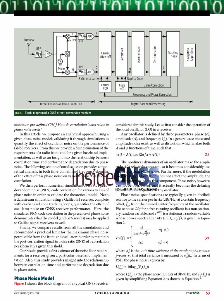
PhaseNoiseModelFigure 1 shows the block diagram of a typical GNSS receiver

considered for this study. Let us first consider the operation of the local oscillator (LO) in a receiver.

Any oscillator is defined by three parameters: phase (φ), amplitude (A), and frequency (f0). In a general case phase and amplitude noise exist, as well as distortion, which makes both A and φ functions of time, such that

(1)

The nonlinear dynamics of an oscillator make the ampli-tude A(t) relatively constant, so it becomes considerably less important than phase noise. Furthermore, if the modulation used to carry information does not affect the amplitude, the receiver can also ignore this component. Phase noise, however, cannot be overlooked, and it actually becomes the defining parameter of the quality of any oscillator.

Phase noise specifications are typically given in decibels relative to the carrier per hertz (dBc/Hz) at a certain frequency offset, fm, from the desired center frequency of the oscillator. Phase noise Φ(t) for a free running oscillator is a non-station-ary random variable, and is a stationary random variable whose power spectral density (PSD), Px(f), is given in Equa-tion 2.

(2)

where is the unit time variance of the random phase noise process, so that total variance is measured by (t). In terms of PSD, the phase noise is given by:

L(fm) = 10log10(Px(fm))

where L(fm) is the phase noise in units of dBc/Hz, and Px(fm) is given by simplifying Equation 2 as shown in Equation 3:

Antenna

BPF

LPF

LPF

Reference carrier Replica Code

Delay Correction

Frequency and Phase Correction

Digital Baseband ProcessingDirect Conversion Radio Front-End

ADC

ADCQ Q Q Q

II I I

CarrierWipe-off

Corre

lato

rs

Accu

mul

ator

s

Disc

rimin

ator

s

Navi

gatio

n Al

gorit

hms

TrackingLoops

LNA

Mixer

Mixer

CarrierNCO

CodeNCO

FIGURE 1 Block-diagram of a GNSS direct-conversion receiver


PhaseNoiseeffects

(3)

and further simplifying phase noise to: (4)

where f0 is the oscillation frequency, fm is the frequency off-set, and σΦ is the constant that defines the noise level of the oscillator. In practice all free-running oscillators show a noise roll-off of 20 decibels per decade when far enough from the fundamental frequency.

The defining assumption of this model is that the phase difference between time instants t1 and t2 follows a Gaussian distribution with null mean and variance linearly increasing with the length of the interval, also known as Wiener or ran-dom-walk processes, thus

(5)

This model is also suitable for PLL-based synthesizers with narrow loop bandwidths where the voltage controlled oscillator (VCO) noise dominates. Even though there are significant differ-

ences in the results when other phase noise models are considered, this can still be considered a first approach to the problem.

PhaseNoiseandcodecorrelationLet us turn now to the factors involved in the effects of phase noise on code correction.

Post-correlationsignaltoNoiseRatio.Letting x(t) be an ideal real signal, having no quadrature component, we initially modulate a carrier at ω0 as x(t)·ejω0t. Complex down-conver-sion, assuming coherent detection, is described by (6):

(6)

where the down-converted signal is then correlated with an aligned replica over a period T. If the code is optimally aligned, Equation 7 results:

(7)

Making several simplifications in the notation, we first normalize the energy of x(t) over T (indicated as |Y|) to 1. Secondly, we assume that x(t) equals {-1,1}, which is true for simple modulations such as binary phase shift keying (BPSK) or binary offset carrier (BOC(m,n)). Finally, we only consider pilot signals, excluding the factor of navigation data. Therefore, in the absence of phase noise,

(8)

Let us now consider the effect of the phase noise of the local oscillator where the carrier is down-converted with an addi-tional random phase φ(t), thus:

(9)

(10)

During the correlation process in a GNSS receiver, this signal is multiplied by an ideal version of itself. Theoretically, when both are perfectly aligned the integral or area of the resulting function is maximized. Calculating the correlation over a period containing phase variations or even inversions results in an energy decrease, because part of the signal is sub-tracted rather than added (or the other way around should the correlation be negative).

In general, phase noise has two effects on the signal. First, the signal may lose energy as the expected value of |Y| decreases with noise, as described in Equation 11. Secondly, the variance of |Y| — ideally 0 — increases, as shown in Equation 12.

(11)

(12)

where μY equals the mean or expected value of |Y| and σY2 equals

the variance of |Y|.

modeling Phase noise effects on receivers: a historyIn1966D.B.Leesonproposedanempiricallinearmodelforthenoisespec-trumofanoscillator,whichhasbeenextensivelycitedintheliteraturesincethen.G.Sauvagegeneralizedthismodeltootherresonantcircuitsin1977,providingadeepermathematicalbackground.In1998A.HajimiriandT.H.Leeproposedalineartimevariantmodel(LTV)toexplaintheeffectofeachofthenoisesourcesofanoscillatoronitsphasenoise.

PhasenoisemodelsforvariouswirelesscommunicationreceivershavebeenproposedbyT.Schenk(2006)(Forthecompletecitationsofthisandotherreferences,pleaseseetheAdditionalResourcessectionneartheendofthemainarticle.)ThearticlebyD.Petrovicet aliausesorthogonalfre-quencydivisionmultiplexing(OFDM)systemsformodelingnoise,whileA.Demiret alia(2000)developedextensiveandgenerictheoryforphasenoisemodels.Ina2002article,Demirextendedthistheorytojitterinopti-calandwirelesscommunications,andK.Kundertalsodevelopedajittermeasurementforphasenoiseeffectsonphaselockedloops.

Asimulation-basedstudyofphasenoiseintroducedbythereceiverandthesatellitepayloadwasdiscussedbyE.Rebeyrolet aliain2006.Derivingthephasenoisepowerspectraldensities,frequencycomparisonsaremade,butcorrelationlossesoreffectsonthecodetrackingloopatthereceiverwerenotincluded.M.IrsiglerandB.Eissfellerdiscusstheimpactofoscilla-torphasenoiseontheperformanceofthePLLtrackingintheir2002article,whilemodelingtheoreticalresults,buttheydrawnoconclusionsregardingthephasenoiserequirementsoftheoscillator.TheiranalysisfocusedonclassificationofthephasenoisesourcesandtypesandonthephaselocklooptrackingperformanceatfixedphasenoiserandomvibrationsandAllandeviations.

In2010,M.Petovelloet aliadiscusstheeffectofresidualphasenoiseinthecarriertrackingloopontheperformanceofC/N0estimationalgorithms,butdonotidentifytheeffectonthecodetrackingloop.A.Demiret alia(2006)providesathoroughanalysisofthespectralcharacteristicsofphasenoise.In2010Schenkdemonstratedthatisastationaryrandomvariabledefinedforafreerunninglocaloscillatorwhosepowerspectraldensity(PSD),Px(f),asgiveninEquation2inthemainarticle.


We can define the post-correlation SNR due to phase noise as the quotient of the square of the mean value of the autocor-relation peak and its variance:

(13)

As the accumulated phase shifts for a given noise level increase, the correlation time also increases. Thus, the inte-grated energy no longer increases linearly with time above cer-tain phase noise levels, and eventually a point may be reached at which phase noise becomes dominant over post-correlation thermal noise, limiting the sensitivity increase one can obtain by increasing the correlation time. We present an explanation of this condition in the following section.

MeanValueofcorrelationPeak.The average magnitude of the correlator output is calculated in order to estimate the noise and losses in the presence of phase noise. Instead of evaluating E[|Y|] we will address E[|Y|2] which provides a similar metric while still allowing an analytical approach. Because noise is assumed to be low, where μY is close to 1, we can easily see that

(14)

In the following paragraphs, we derive the relation between front-end oscillator phase noise and peak value of code corre-lation, using theoretical and analytical means in the time and frequency domains, respectively.

First, in the time domain, from Equation 11 we have,

(15)

(16)

We define the probability density function of the phase as

If t2>t1, then

and due to odd symmetry:

Conversely, if t1>t2, then:

(17)

Following a similar approach it can be seen that

(18)

and, therefore,

(19)

These losses due to noise are a function of TσΦ2, which is

the phase noise variance over one code epoch (σΦ2 is the rate at

which the variance of the oscillator phase increases with time; so, TσΦ

2 happens to be the phase variance at t=T). This follows intuitively because the variance of the phase increases linearly with time, which means scaling this phase noise has the same effect as applying this factor to the correlation time. For small values of TσΦ

2 the following approximation can be made:

(20)

(21)

In the frequency domain we can derive a theoretical expres-sion for correlation losses using a free-running oscillator model in the RF front-end PLL. We assume that the PRN code is c(t). For the sake of simplicity, we also assume that noise and mul-tipath effects are absent.

The complex PRN code correlation output R(τ) at the receiv-er is obtained by correlating the incoming down-converted signal with a local reference code delayed by τ seconds. If we take into account the phase noise of the local oscillator, the correlation output can be written as:

(22)

whereejΦ(t) = time-dependent phase noise effect,c*(t-τ) = time-delayed local code,Φ(t) = non-stationary random variable modeling the phase

noise effect, andT = pre-detection integration time (PIT) over which code

correlation is performed. (Note that T and PIT are the same, except that T is used in mathematical formulations and PIT in theoretical explanations; so, they should be mutually inter-changeable.)

FIGURE 2 Equivalent model of phase noise effect.

h(t)Integrator over T

X Y

e jΦ(t) ( e dt)jΦ(t)T

0 0


The correlation peak has maximum value at R(0) when the time delay between the incoming signal and the local replica is zero, in other words, when the two signals are perfectly aligned in time domain, as expressed by Equation 23:

(23)

We have considered |c(t)|2 equals 1 because the PRN code c(t) is essentially a binary sequence of +1s and -1s. Equation 23 shows that the correlation peak fluctuates randomly, accord-ing to Φ(t), and also shows that the effect of correlation peak in the presence of noise can be modeled as a filtered random variable X = ejΦ(t) passed through an integrator filter, as shown in Figure 2.

The integrator impulse response is a rectangular pulse of width T:

(24)

Therefore, its frequency response is given by the well-known sinc function:

(25)

The PSD of the input X from Figure 2 is given in Equation 2. Because X is a stationary random variable and h(t) is linear filter, the PSD of the output random process Y (which corre-sponds to the fluctuations of the correlation peak R(0) ) is given by Equation 26):

(26)

The average power of the correlation peak is E(R2(0)) equals E(Y2) and will be therefore calculated by integrating the PSD of Y over the whole frequency axis, as shown in equations 27 and 28:

(27)

where equals 0 indicates absence of phase noise. The integral in Equation 27 for not equal to 0 has been evaluated and its closed form expression is given by Equation 29:

(29)

The mean value of correlation peak in presence of phase noise is therefore obtained by dividing Equation 29 by Equa-tion 28:

(30)

The loss or deterioration in correlation peak due to phase noise will be the inverse of Equation 30. This is, as expected, exactly the same result as that obtained by using the time domain analysis.

correlationNoise. Signal losses due to phase variations dur-ing correlation already give the lower boundary for the phase noise specification. But this lower boundary alone does not represent the actual degradation of system performance.

It is reasonable to expect strong variations in the constella-tion (correlation noise) before the loss due to phase noise out-weighs losses due to other factors in the receiver chain. The variance of the correlation peak, described by Equation 31, must be studied as well.

(31)

Unfortunately, even though the first order approximation, given in Equation 14, is accurate enough to estimate losses, it is not a valid for obtaining σY. However, because no analytical expression has been found for μY, numerical approximations have been made in order to estimate σY.

In the presence of relatively low noise levels, σY increases lin-early with TσΦ

2. Adjusting the scale factor through simulations and defining the noise power (PN) logarithmically as PN equals 20 log10(σY) , we obtain the variance of the correlation peak:

(32)

SNRPN can now be estimated as long as noise is low enough for this first-order approximation to remain valid. Figure 3 shows that this approximation is appropriate where TσΦ

2 less than 1.

ModelforcorrelationBetweenPhaseNoiseandPurePRNcodesIn the previous section describing the effect of phase noise on code correlation, we derived a relation between front-end oscil-lator phase noise and peak value of code correlation in the time

PhaseNoiseeffects

FIGURE 3 Variance of correlation peak.

SimulationsApproximation

20lo

g10(σγ

)

100

50

0

-50

-100

-150

ΦTσ210-3 10-2 10-1 10 101 102

(28)


and frequency domains, respectively. The next step is to prove this relation using a software-generated, simulation-based model of the code correlation process.

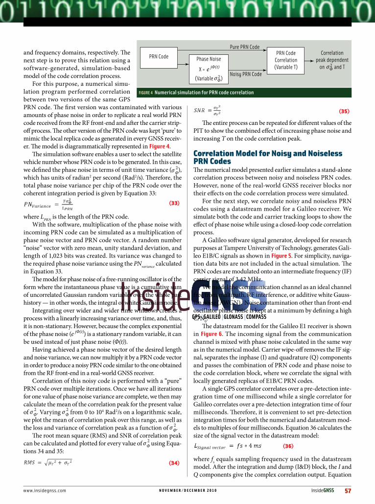
For this purpose, a numerical simu-lation program performed correlation between two versions of the same GPS PRN code. The first version was contaminated with various amounts of phase noise in order to replicate a real world PRN code received from the RF front-end and after the carrier strip-off process. The other version of the PRN code was kept ‘pure’ to mimic the local replica code as generated in every GNSS receiv-er. The model is diagrammatically represented in Figure 4.

The simulation software enables a user to select the satellite vehicle number whose PRN code is to be generated. In this case, we defined the phase noise in terms of unit time variance ( ), which has units of radian2 per second (Rad2/s). Therefore, the total phase noise variance per chip of the PRN code over the coherent integration period is given by Equation 33:

(33)

where LPRN is the length of the PRN code. With the software, multiplication of the phase noise with

incoming PRN code can be simulated as a multiplication of phase noise vector and PRN code vector. A random number “noise” vector with zero mean, unity standard deviation, and length of 1,023 bits was created. Its variance was changed to the required phase noise variance using the PNvariance calculated in Equation 33.

The model for phase noise of a free-running oscillator is of the form where the instantaneous phase value is a cumulative sum of uncorrelated Gaussian random variables over the whole past history — in other words, the integral of white Gaussian noise.

Integrating over wider and wider time windows creates a process with a linearly increasing variance over time, and, thus, it is non-stationary. However, because the complex exponential of the phase noise ( ) is a stationary random variable, it can be used instead of just phase noise (Φ(t)).

Having achieved a phase noise vector of the desired length and noise variance, we can now multiply it by a PRN code vector in order to produce a noisy PRN code similar to the one obtained from the RF front-end in a real-world GNSS receiver.

Correlation of this noisy code is performed with a “pure” PRN code over multiple iterations. Once we have all iterations for one value of phase noise variance are complete, we then may calculate the mean of the correlation peak for the present value of . Varying from 0 to 104 Rad2/s on a logarithmic scale, we plot the mean of correlation peak over this range, as well as the loss and variance of correlation peak as a function of .

The root mean square (RMS) and SNR of correlation peak can be calculated and plotted for every value of using Equa-tions 34 and 35:

(34)

(35)

The entire process can be repeated for different values of the PIT to show the combined effect of increasing phase noise and increasing T on the code correlation peak.

correlationModelforNoisyandNoiselessPRNcodesThe numerical model presented earlier simulates a stand-alone correlation process between noisy and noiseless PRN codes. However, none of the real-world GNSS receiver blocks nor their effects on the code correlation process were simulated.

For the next step, we correlate noisy and noiseless PRN codes using a datastream model for a Galileo receiver. We simulate both the code and carrier tracking loops to show the effect of phase noise while using a closed-loop code correlation process.

A Galileo software signal generator, developed for research purposes at Tampere University of Technology, generates Gali-leo E1B/C signals as shown in Figure 5. For simplicity, naviga-tion data bits are not included in the actual simulation. The PRN codes are modulated onto an intermediate frequency (IF) carrier signal of 3.42 MHz.

We model the communication channel as an ideal channel free from multipath, RF interference, or additive white Gauss-ian noise (AWGN). Noise contamination other than front-end oscillator phase noise is kept at a minimum by defining a high C/N0.

The datastream model for the Galileo E1 receiver is shown in Figure 6. The incoming signal from the communication channel is mixed with phase noise calculated in the same way as in the numerical model. Carrier wipe-off removes the IF sig-nal, separates the inphase (I) and quadrature (Q) components and passes the combination of PRN code and phase noise to the code correlation block, where we correlate the signal with locally generated replicas of E1B/C PRN codes.

A single GPS correlator correlates over a pre-detection inte-gration time of one millisecond while a single correlator for Galileo correlates over a pre-detection integration time of four milliseconds. Therefore, it is convenient to set pre-detection integration times for both the numerical and datastream mod-els to multiples of four milliseconds. Equation 36 calculates the size of the signal vector in the datastream model:

(36)

where fs equals sampling frequency used in the datastream model. After the integration and dump (I&D) block, the I and Q components give the complex correlation output. Equation

FIGURE 4 Numerical simulation for PRN code correlation

PRN Code

Pure PRN Code

Noisy PRN Code

PRN CodeCorrelation(Variable T)

Correlationpeak dependent

on and TPhase Noise

X =

(Variable )σ2Φ

σ2Φe jΦ(t)


37 is used to calculate the normalized magnitude of correlation peak:

(37)

where, C equals magnitude of correla-tion, I equals In-phase component of correlation output, Q equals quadra-ture component of correlation output. If PIT is selected as the nth multiple of four milliseconds, the correlation output vector has n elements, and the total value of correlation peak is then a cumulative sum of all n values.

Similar to the numerical model, in the datastream model the phase noise variance is also varied from 0 to 104 Rad2/s on a logarithmic scale. Mean, loss, and variance of correlation peak are measured while RMS and SNR are calculated and plotted against . We carried out these simulations for PITs of 4, 8, 12, 20, and 100 milliseconds.

ResultsandMathematicalinterpretationFigure 7 shows the plot for the loss of correlation peak versus phase noise variance per unit time ( ) for various values of the PIT for the analytical (the-oretical), numerical, and datastream models. Figures 8 and 9 show the vari-ance and the RMS of the correlation peak versus .

Similarly, Figure 10 shows the SNR of correlation peak, while for simplicity only the results for intervals of 4, 12, and 100 milliseconds are plotted for the vari-ance and SNR.

(A comparison between the theoreti-cal model and the simulation models for variance of correlation peaks was already shown in Figure 3.) . The results illus-trate the validity of the simulation for a stand-alone, open-looped correlation process, even in a real-world receiver with fully functional carrier and code tracking loops.

Figure 7 indicates that the loss in correlation peak increases as phase noise increases. However, for larger T inter-vals, where for a particular , the loss in correlation peak is larger. The maximum variance of correlation is approximately –13 decibels irrespective of T, but this

maximum is reached at lower values of with increasing T. This result is con-

sistent with the explained interchange-ability of T and in the expressions for this correlation degradation.

As PNvariance increases, the mean

and RMS of the correlation peak fall. The variance of the correlation peak increases up to a certain maximum and then also falls, but this decrease is in the region where the losses are already unsustainable. This result is

PhaseNoiseeffects

FIGURE 6 Galileo E1 receiver model

X

2Inc sig

1tracking_en

est carrierphase error

est carrierphase error

Ichannel

Qchannel

E1B replica

E1C replica

trigger signal

nco phase

tracking_en

carrierwipe-off

Add Code nco+ +

Dual Channel Correlation and discriminators

Product

Subsystem

XProduct 1

In1Out1z-1 z-1

Code NCOand PRN

generator

In1 I channel

Q channelIn2

FIGURE 5 Galileo E1B/C signal generator shown schematically in datastream simulation

Navi_bit

Navigation Bit

IF Signal

Intermediate frequency

E1B

Primary Code E1B

BOC11

SinBOC(1,)Subcarrier

BOC61

SinBOC(6,1)Subcarrier

E1C

Primary Code E1C

CS25

E1C Secondary Code

Zero-OrderHold1

Zero-OrderHold1

K

Alpha

K

Beta

X

P5

X

P3

X

P1X

P2

X 1

P4 Out1

++

-+

-+

Add

Subtract

94


reasonable, because the value of the correlation peak con-verges to zero.

Increasing the PIT above four mi l l iseconds is a lso detrimental to the correlation output, because al l the negative observations due to an increase in PNvariance begin at lower values of σ Φ

2. In other words, the maxi-mum allowable input PNvariance for a certain level of correlation peak RMS progressively decreases as we increase the PIT.

In the numerical and datastream simulations, an effective approach for identifying the maximum phase noise is to use a free-running local oscillator phase noise model, with a 10-deci-bel minimum correlation output SNR. Although these bound-aries for the SNR criteria seem very stringent, we plan to use more realistic, practical models in which phase noise flattens below a given frequency offset. We expect that this condition will, in turn, modify the slope of the SNR so that the synthe-sizer requirements would become closer to the figures offered by real receivers.

In Figure 10, in order to maintain a minimum correlation SNR of 10 decibels when the PIT is 4 milliseconds, the maxi-mum allowable is 251.2. For a PIT of 100 milliseconds, the maximum allowable to maintain a similar correlation SNR is 15.5. Using Equation 4, with a 4-millisecond PIT and fre-quency offset (fm) of one megahertz, the maximum allowed phase noise is

(38)

Similarly, for a PIT of 100 milliseconds, PNmax is -124 dBc/Hz, which means that, for longer integration intervals, phase noise requirements from front-end local oscillator become more stringent.

Figures 11 and 12 show the datastream simulation plots for the RMS and SNR of correlation peak in presence of multipath effects and additive white Gaussian noise (AWGN) channel imperfections. Two multipath components of half the power of

PhaseNoiseeffects

FIGURE 7 Loss of correlation peak versus phase noise variance (PIT: black = 4 milliseconds, red = 8 milliseconds, blue = 12 milliseconds, magenta = 20 milliseconds, green = 100 milliseconds).

Simulated - MatlabSimulated - SimulinkTheoretical

Loss

of c

orre

latio

n pe

ak (d

B)

50

40

30

20

10

0

PN Variance per unit time Φ2(σ )

101 102 103 104

FIGURE 8 Variance of correlation peak versus phase noise variance (PIT: black=4 milliseconds, blue=12 milliseconds, green=100 milliseconds).

Simulated - MatlabSimulated - Simulink

Varia

nce o

f cor

rela

tion

peak

(dB)

-10

-20

-30

-40

-50


101 102 103 104

FIGURE 9 Figure 9 RMS of correlation peak versus phase noise variance (PIT: black = 4 milliseconds, red = 8 milliseconds, blue = 12 milliseconds, magenta = 20 milliseconds, green = 100 milliseconds)


RMS o

f cor

rela

tion

peak

(dB)

0

-5

-10

-15

-20

-25


101 102 103 104

FIGURE 10 SNR of correlation peak versus σΦ2 (PIT: black =4 milliseconds,

blue =12 milliseconds, green =100 milliseconds)


SNR

of co

rrela

tion

peak

(dB)

50

40

30

20

10

0

-10


101 102 103 104


the line of sight (LOS) component with delays of one chip and half chip, respec-tively, were added to the LOS compo-nent. AWGN was added such that over-all carrier-to-noise ratio reduced by 25 decibels. For comparison, the numerical simulation results, absent the effects of multipath and AWGN, are also provided in the same figures.

Channel imperfections only result in a fixed attenuation of the overall RMS characteristics, in this case 12 decibels.

However, the shape of the curves and, hence, the effects of phase noise, remain unchanged. This can be easily demon-strated by compensating the datastream model curves with +12 decibels so that they match perfectly with the numerical model curves as shown in Figure 11.

In the case of SNR, the difference between curves with and without chan-nel imperfections is higher for lower values of integration intervals and phase noise. This occurs because, as the inte-

gration interval, T, and PN increase, the SNR of correla-tion drops anyway, blunting the effect of channel imper-fections.

Figure 13 repre-sents the SNR due

to phase noise (SNRPN), as a function of TσΦ

2 obtained after fitting with numeri-cally computed data. For a given correla-tion time T, we can immediately obtain the maximum acceptable noise level σΦ required to achieve a certain SNR or, conversely, the maximum acceptable integration interval T under a given noisy oscillator.

Regarding the latter, it is interesting to note that SNR due to thermal noise, SNRTH, increases with integration time, while SNR due to phase noise under this model does exactly the opposite as shown in Figure 14. This limit is especially important in high-sensitiv-ity receivers where integration periods are long, due to the quality of the local oscillator setting a boundary beyond which SNR can no longer be improved through coherent integration.

FIGURE 11 RMS of correlation peak in presence of multipath & AWGN (PIT: black =4 milliseconds, blue =12 milliseconds, green =100 milliseconds)

Without Multipath & AWGNWith Multipath & AWGN (compensated by +12dB)

RMS o

f cor

rela

tion

peak

(dB)

0

-5

-10

-15

-20

-25


101 102 103 104

FIGURE 12 . SNR of correlation peak in presence of multipath & AWGN (PIT: black =4 milliseconds, blue =12 milliseconds, green =100 milliseconds)

Without Multipath & AWGNWith Multipath & AWGN

SNR

of co

rrela

tion

peak

(dB)

40

30

20

10

0


101 102 103 104

FIGURE 13 SNRPN as a function of TσΦ2

SNR PN

(dB)

40

30

20

10

0

T Φ2σ

10-1 100 101

FIGURE 14 Thermal and phase noise contributions to SNR

SNR(

dB)

40

30

20

10

0

T(ms)10-1 100 101

SNRPNSNRTHSNR

PhaseNoiseeffects

Maximum Phase Noise (dBc/Hz)

PIT(milliseconds) fm=10(kilohertz) fm=1(megahertz)

T=4 -72 -112

T=12 -74 -114

T=100 -84 -124

TABLE 1. Maximum phase noise in order to maintain a minimum correlation SNR of 10 decibels for different values of PIT and fm


Let us consider for example the case of GPS L1 C/A with a nominal SNR ther-mal or SNRTH of 34 decibels for a T of 20 milliseconds, representing the worst case for phase noise. As thermal noise is minimal, the phase noise becomes a lim-iting factor sooner. If we set equals 100, the combined SNR is:

(39)

Figure 14 clearly shows how the SNR increases with the correlation interval until the phase noise becomes domi-nant, under the assumption of negli-gible phase noise losses, compressing the SNRTH curve. The optimal T in this case falls below 20 milliseconds, indicat-ing non-coherent integration methods would be more appropriate under these assumptions.

conclusionThis phase model is a conservative first approximation, illustrating the rela-tionships between phase noise, ther-mal noise, and correlator performance. In this article, we first presented an analytical approach for evaluating the effects of the local oscillator phase noise in the performance of the correlators of a GNSS receiver. A mathematical model validated the analytical approach, and a datastream model demonstrated the tracking channel imperfections based on GNSS receiver implementations

We characterized the relationship between the integration time and phase noise, and presented a criterion for radio front-end design. We believe this model offers new tools for the analytical design of GNSS receivers, while laying a con-servative boundary for their practical design.

acknowledgmentsThe research leading to these results has received funding from the Euro-pean Community Seventh Framework Program (FP7/2007-2013) under grant agreement number 227890. This work has also been supported by the Academy of Finland.

ManufacturersThe analytical portion of this study was

developed using Maple from Maplesoft, Waterloo, Ontario, Canada. The numer-ical model was developed using Mat-lab, and the datastream model utilized Simulink, both from The Mathworks, Natick, Massachusetts, USA.

additionalResources[1]Demir,A.,“PhaseNoiseandTimingJitterinOscillatorsWithColored-NoiseSources,”IEEETransactions on Circuits and Systems- Funda-mental Theory and Application,Vol.49,No.12,December2002

[2]Demir,A.,andA.MehrotraandJ.Roychowd-hury,“PhaseNoiseinOscillators:aUnifyingThe-oryandNumericalMethodsforCharacterization,”IEEE Transactions on Circuits and Systems I: Fun-damental Theory and Applications,Vol.47,No5,May2000,pp.655–674,DOI10.1109/81.847872

[3]Hajimiri,A.,andT.H.Lee,“Ageneraltheoryofphasenoiseinelectricaloscillators”,IEEEJ.Solid-StateCircuits,vol.33,pp.179-194,Febru-ary1998

[4]Irsigler,M.,andB.Eissfeller,“PLLTrackingPerformanceinthePresenceofOscillatorPhaseNoise,”GPS Solutions,Volume5(4),pp.45-57,Spring2002

[5]Kundert,K.,“PredictingthePhaseNoiseandJitterofPLL-BasedFrequencySynthesizers,”,TheDesigner’sGuideCommunity<www-designers-guide.org>,Designer’sGuideConsultingInc.,August2006

[6]Leeson,D.B.,“Simplemodeloffeedbackoscillatornoisespectrum,”ProceedingsIEEE,p.369,February1966

[7]Petovello,M.,andE.Falletti,M.Pini,andL.Presti,“AreCarrier-to-NoiseAlgorithmsEquiva-lentinAllSituations?”GNSSSolutions,Inside GNSS,pp.20-27,January/February2010

[8]Petrovic,D.,andW.RaveandG.Fettweis,“EffectsofPhaseNoiseonOFDMSystemsWithandWithoutPLL:CharacterizationandCompensa-tion,”IEEE Transactions on Communications,Vol.55,No.8,Aug2007

[9]Rebeyrol,E.,andC.Macabiau,L.Ries,J-L.Issler,M.Bousquet,andM-L.Boucheret,“PhaseNoiseinGNSSTransmission/ReceptionSystem,”Proceedings of the 2006 National Technical Meet-ing of the Institute of Navigation,January18–20,2006,Monterey,California,USA

[10]Sauvage,G.,“PhaseNoiseinOscillators:AMathematicalAnalysisofLeeson’sModel,”IEEETransactionsonInstrumentationandMeasure-ment,Vol.IM-26,No.4,December1977

[11]Schenk,T.,“PhaseNoise,”Chapter4ofRF Imperfections in High-rate Wireless Systems,ISBN:978-1-4020-6902-4,Springer2008

[12]Schenk,T.(2006),“RFImpairmentsinMul-tipleAntennaOFDM–InfluenceandMitigation,”Ph.D.Thesis,TechnicalUniversityofEindhoven,November2006

[13]Syrjälä,V.andM.Valkama,“Analysisandmit-igationofphasenoiseandsamplingjitterinOFDMradioreceivers,”EuropeanMicrowaveAssociation,International Journal of Microwave and Wireless Technologies,vol.2,pp.193-202,April2010

[14]Syrjälä,V.,andM.Valkama,N.N.Tchamov,andJ.Rinne,“PhaseNoiseModellingandMiti-gationTechniquesinOFDMCommunicationSys-tems,” Wireless Telecommunication Symposium,WTS2009,April2009,pp.1-7

authorsErnesto Pérez Sernaobtained his M.Sc.degreeintelecommuni-cationsengineeringattheUniversityofCanta-bria(Spain),wherehelaterworkedwithinthe

DepartmentofCommunicationsEngineering(DICOM)from2005to2006,designingSiGeandSiCMOSPLLfrequencysynthesizersforRFreceiv-ers.HejoinedACORDEin2006asR&Dengineer,mainlydesigningcustomCMOSRFanddigitalICsforGNSSapplications.HehasbeeninvolvedinalltheASICdesignsoftheFP6GREATprojectandtheMAGNETBEYONDtransmitterandhaspublishedseveralpapersintheareaofMMICdesign.Heiscurrentlyworkingtowardshismaster’sdegreeininformationtechnologyandmobilecommunica-tionsandaPh.D.intelecommunicationsattheUniversityofCantabria.

Sarang ThombrereceivedhisB.Sc.degree(withDistinction)inelectron-icsandtelecommunica-tionsengineering(E&TC)fromUniversityofPune(UoP), India and his

M.Sc.degree(withDistinction)fromTampereUniversityofTechnology(TUT),Finlandinradiofrequencyelectronics.Currently,heisworkingasaresearcherandPh.D.studentwiththeDepart-mentofComputerSystemsatTUT,Finland.HisgeneralresearchinterestsareinsoftwarebasedsimulationofGNSSsignalsanddesignandanaly-sisofradiofront-endsforGNSSreceivers.

Mikko Valkamareceivedthe M.Sc. and Ph.D.degrees(bothwithhon-ors)inelectricalengi-neering(EE)fromTam-pere University ofTechnology(TUT),Fin-

land.In2002hereceivedthe“BestPh.D.Thesis”

PhaseNoiseeffects


awardfromtheFinnishAcademyofScienceandLettersforhisdissertationentitled“AdvancedI/Qsignalprocessingforwidebandreceivers:Modelsandalgorithms.”Currently,heisafullprofessorintheDepartmentofCommunicationsEngineeringatTUT.Hisgeneralresearchinterestsincludecom-municationssignalprocessing,estimationanddetectiontechniques,signalprocessingalgo-rithmsforsoftwaredefinedandcognitiveradios,differentsamplingmethodsincludingcompres-sivesampling,digitaltransmissiontechniquessuchasdifferentvariantsofmulticarriermodula-tionmethodsandOFDM,andradioresourceman-agementforad-hocandmobilenetworks.

Simona LohanhasbeenanadjunctprofessorintheDepartmentofCommu-nicationsEngineering,TampereUniversityofTechnologysince2007.SheobtainedherPh.D.

degreeinwirelesscommunicationsfromTampereUniversityofTechnologyandalsograduatedwithanM.Sc.inelectricalengineeringfrom“Politehni-ca”UniversityofBucharest,Romania,andwithaD.E.A.(Frenchequivalentofmaster’sdegree)ineconometricsfromEcolePolytechnique,Paris,France.Lohaniscurrentlyleadingtheresearchactivitiesinsignalprocessingforwirelesscom-municationsintheDepartmentofCommunica-tionsEngineering,TUT.Sheistheprincipalinves-tigator in a research project funded by theAcademyofFinlandfocusingonindoorlocationandhasbeeninvolvedastechnicalgroupleaderintwoEuropeanGNSS-relatedprojects,withinFP6andFP7:“GREAT”and“GRAMMAR,”dealingwithGalileomass-marketreceivers.

Ville SyrjäläreceivedtheM.Sc.degree(withhon-ors)incommunicationsengineering (CS/EE)fromTampereUniversityof Technology (TUT),Finland.Currently,heis

workingasaresearcherwiththeDepartmentofCommunicationsEngineeringatTUT,Finland.Hisgeneralresearchinterestsareincommunicationssignalprocessingandsignalprocessingalgo-rithmsforflexibleradios.

Marco DetrattireceivedtheLaureadegree(M.Sc.)inelectronicengi-neeringfromtheUniver-sityofPerugia(Italy)andtheDEA(DiplomaofAdvancedStudies)from

theUniversityofCantabria(Spain).HejoinedACORDEin2005todevelopcustomRFsolutionsforsatelliteapplications.Atpresentheisleading

theGNSSdepartmentandisinchargeofthedevelopmentofnavigationproductsandRFequipmentwithinthecompanyportfolio.Detrat-tihasbeenthe“responsible”oftheASICfront-enddevelopmentswithinFP6GREATProjectandoftheplatformoftheFP6MAGNET/BEYONDproj-ect.AtpresentheisactingastechnicalmanageroftheFP7GRAMMARprojectforthedevelopmentofanadvancedmulti-frequencyGNSSreceiver.

H e i k k i H u r s k a i n e nreceivedanM.Sc.degreeinelectricalengineeringanddoctoraldegreeincomputingandelectricalengineeringfromTam-pereUniversityofTech-

nology(TUT),Findland.Currently,HurskainenisworkingasaresearchfellowatTUT’sDepartmentofComputerSystems,wherehecontinuestoworkinsatellitenavigationresearchprojects.Hisresearchinterestsinclude,butarenotrestrictedto,evolutionofGNSSes,implementationandpro-totyping issues of receiver algorithms, andemergingapplicationsofGNSSreceivers.

Jari NurmiisaprofessorofcomputersystemsatTampereUniversityofTechnology(TUT),whereobtainedaPh.D.degreeand currently leads agroup of about 20

researchers.Hehasheldvariousresearch,educa-tionandmanagementpositionsatTUTandintheindustrysince1987.Hiscurrentresearchinterestsincludesystem-on-chipintegration;embeddedandapplication-specificprocessor,multiproces-sorandreconfigurablearchitectures;andcircuitimplementationsofpositioning,DSP,anddigitalcommunicationsystems(includingsoftware-definedradioapproach).NurmiisthegeneralchairmanoftheannualInternationalSymposiumonSystem-on-Chip(SoC)anditspredecessorSoCSeminarinTamperesince1999andisnoweditingSpringerbooksonGalileo Positioning Technology and Computation Platforms for SDR.In2004,hewasoneoftherecipientsofNokiaEducationalAward,andtherecipientofTampereCongressAward2005.

PhaseNoiseeffects

local oscillator phase noise effects - inside gnssinsidegnss.com/auto/novdec10-thombre.pdf ·...

Documents