local labor markets$ - university of california, berkeley
TRANSCRIPT

CHAPTER1414Local Labor MarketsI
Enrico MorettiUC Berkeley, NBER, CEPR and IZA
Contents1. Introduction 12382. Some Important Facts about Local Labor Markets 1242
2.1. Nominal wages 12432.2. Real wages 12492.3. Productivity 12512.4. Innovation 1253
3. Equilibrium in Local Labor Markets 12543.1. Spatial equilibrium with homogeneous labor 1257
3.1.1. Assumptions and equilibrium 12573.1.2. Effect of a labor demand shock on wages and prices 12603.1.3. Incidence: who benefits from the productivity increase? 12633.1.4. Effect of a labor supply shock on wages and prices 1264
3.2. Spatial equilibrium with heterogenous labor 12653.2.1. Assumptions and equilibrium 12663.2.2. Effect of a labor demand shock on wages and prices 12673.2.3. Incidence: changes in wage and utility inequality 1270
3.3. Spatial equilibrium with agglomeration economies 12733.4. Spatial equilibrium with tradable and non-tradable industries 12763.5. Some empirical evidence 1278
4. The Determinants of Productivity Differences Across Local Labor Markets 12814.1. Empirical estimates of agglomeration economies 12824.2. Explanations of agglomeration economies 1286
4.2.1. Thick labor markets 12864.2.2. Thick market for intermediate inputs 12904.2.3. Knowledge spillovers 1291
5. Implications for Policy 12965.1. Equity considerations 1297
5.1.1. Incidence of subsidies 12975.1.2. Taxes and transfers based on nominal income 13015.1.3. Nominal and real differences across skill groups and regions 13015.1.4. Subsidies to human capital when labor is mobile 1303
I This research was funded by a grant from the University of Kentucky Center on Poverty Research. I am grateful toGiacomo De Giorgi, Craig Riddell, Issi Romen, Michel Serafinelli, David Wildasin, the editors and especially Pat Klineand Gilles Duranton for useful comments on an earlier version. I thank Ana Rocca for excellent research assistance. Ithank Richard Hornbeck for help with the data on total factor productivity from the Census of Manufacturers. Anyopinions and conclusions expressed herein are those of the author and do not necessarily represent the views of theUS Census Bureau. All results based on data from the Census of Manufacturers have been reviewed to ensure that noconfidential information is disclosed.
Handbook of Labor Economics, Volume 4b ISSN 0169-7218, DOI 10.1016/S0169-7218(11)02412-9c© 2010 Elsevier Ltd. All rights reserved. 1237
1238 Enrico Moretti
5.2. Efficiency considerations 13045.2.1. Internalizing agglomeration spillovers 13045.2.2. Unemployment, missing insurance and credit constraints 1307
6. Conclusions 1308References 1309
AbstractI examine the causes and the consequences of differences in labor market outcomes across locallabor markets within a country. The focus is on a long-run general equilibrium setting, whereworkers and firms are free to move across localities and local prices adjust to maintain the spatialequilibrium. In particular, I develop a tractable general equilibrium framework of local labor marketswith heterogenous labor. This framework is useful in thinking about differences in labor marketoutcomes of different skill groups across locations. It clarifies how, in spatial equilibrium, localizedshocks to a part of the labor market propagate to the rest of the economy through changes inemployment, wages and local prices and how this diffusion affects workers’ welfare. Using thisframework, I address three related questions. First, I analyze the welfare consequences of productivitydifferences across local labor markets. I seek to understand what happens to the wage, employmentand utility of workers with different skill levels when a local economy experiences a shift in theproductivity of a group of workers. Second, I analyze the causes of productivity differences across locallabor markets. To a large extent, productivity differences within a country are unlikely to be exogenous.I review the theoretical and empirical literature on agglomeration economies, with a particular focuson studies that are relevant for labor economists. Finally, I discuss the implications for policy.
Keywords: Cities; Wage; General equilibrium; Spatial equilibrium
1. INTRODUCTIONLocal labor markets in the US are characterized by enormous differences in workerearnings, factor productivity and firm innovation. The hourly wage of workers locatedin metropolitan areas at the top of the wage distribution is more than double the wageof observationally similar workers located in metropolitan areas at the bottom of thedistribution. These differences reflect, at least in part, variation in local productivity. Forexample, total factor productivity of manufacturing establishments in areas at the top ofthe TFP distribution is three times larger than total factor productivity in areas at thebottom of the distribution. The amount of innovation is also spatially uneven. Firmsin Santa Clara and San Jose generate respectively 3390 and 1906 new patents in a typicalyear, while the median city generates less than 1 patent per year. Notably, these differencesin wages, productivity and innovation appear to be largely persistent over the last threedecades.
In this chapter, I review what we know about the causes and the consequences ofdifferences in labor market outcomes across local labor markets within a country. Thefocus is on a long-run general equilibrium setting, where workers and firms are freeto move across localities and local prices adjust to maintain the spatial equilibrium. Inparticular, I develop a tractable general equilibrium framework of local labor markets

Local Labor Markets 1239
with heterogenous labor. This framework—which represents the unifying theme of thechapter—is useful in thinking about differences in labor market outcomes of differentskill groups across locations. It clarifies how, in spatial equilibrium, localized shocks toa part of the labor market propagate to the rest of the economy through changes inemployment, wages and local prices and how this diffusion affects workers’ welfare.
Using this framework, I address three related questions.
1. First, I analyze the welfare consequences of productivity differences across local labormarkets. I seek to understand what happens to the wage, employment and utility ofworkers with different skill levels when a local economy experiences a shift in theproductivity of a group of workers. I focus on welfare incidence and use the spatialequilibrium model to clarify who ultimately benefits from permanent productivityshocks.
2. Second, I analyze the causes of productivity differences across local labor markets. Toa large extent, productivity differences within a country are unlikely to be exogenous.I review the theoretical and empirical literature on agglomeration economies, with aparticular focus on studies that are relevant for labor economists.
3. Finally, I discuss the implications for policy, with a special focus on location-basedeconomic development policies aimed at creating local jobs. I clarify when thesepolicies are wasteful, when they are efficient and who the expected winners and losersare.
The topic of local labor markets should be of great interest to labor economists fortwo reasons. First, the issue of localization of economic activity and its effects on workers’welfare is one of the most exciting and promising research grounds in the field. This area,at the intersection of labor and urban economics, is ripe with questions that are both offundamental importance for our understanding of how labor markets operate and havedeep policy implications. Why are some cities prosperous while others are not? Given thatfactors of production can move freely within a country, why do firms locate in expensivelabor markets? What are the ultimate effects of these differences on workers’ welfare?These questions have intrigued economists for more than two centuries, but it is only inthe last three decades that a body of high quality empirical evidence has begun to surface.The pace of empirical research in this area has accelerated in the last 10-15 years. It isa topic whose relative importance within the field of labor economics promises to keepgrowing in the next decade.
Second, and more generally, the issue of equilibrium in local labor markets shouldbe of broader interest for all labor economists, even those who are not directlyinterested in economic geography per se. With notable exceptions, labor economists havetraditionally approached the analysis of labor market shocks using a partial equilibriumanalysis. However, a partial equilibrium analysis misses important parts of the picture,since the endogenous reaction of factor prices and quantities can significantly alterthe ultimate effects of a shock. Because aggregate shocks to the labor market are

1240 Enrico Moretti
rarely geographically uniform, the geographic reallocation of factors and local priceadjustments are empirically important. It is difficult to fully understand aggregate labormarket changes—like changes in relative wages or employment—if ignoring the spatialdimension of labor markets. Partial equilibrium analyses can be particularly misleading inthe case where the workforce is highly mobile, like in the US. Labor flows across localitiesand changes in local prices have the potential to undo some of the direct effects of labormarket shocks. This can profoundly alter the implications for policy. In this respect, theworkings of local labor markets and their spatial equilibrium cannot be overlooked bylabor economists, even those who are working on more traditional topics like wagedetermination, wage inequality or unemployment.
As an example, consider a nationwide increase in the productivity of skilledworkers in an industry, say the software industry. Although the shock is nationwide, itaffects different local labor markets differently because the software industry—like mostindustries—is spatially concentrated. The effect on the demand for skilled labor in a citylike San Jose–in the heart of Silicon Valley—is likely to be quite different from the effectin a city like Phoenix—where the software sector is nonexistent. In a partial equilibriumsetting, the only effect of this shock is an increase in the nominal wage of skilled workersin San Jose. However, in general equilibrium this shock propagates to other parts of theeconomy through changes in factor prices and quantities. Indeed, in general equilibrium,all agents in the economy are affected, irrespective of their location and their skill level.Attracted by higher demand, some skilled workers leave Phoenix and move to San Jose,thus pushing up the cost of housing and other non-tradable goods there. Unskilledworkers in San Jose are affected because cost of living increases and because of imperfectsubstitution between skilled and unskilled labor. On net, some unskilled workers moveto Phoenix, attracted by higher real wages. Skilled and unskilled workers in Phoenix alsoexperience changes in their equilibrium wage, even if their productivity has not changed,because of changes in their local supply. Following population changes, owners of landexperience changes in the value of their asset, both in San Jose and Phoenix. In thisexample, the direct effect of the demand shock is partially offset by general equilibriumchanges due to worker relocation and local price adjustments. The ultimate change in thenominal and real wage of skilled and unskilled workers—and their policy implications—are quite different from the partial equilibrium change and crucially depends on thedegree of labor mobility and the magnitude of local prices changes.
The chapter proceeds as follows. I begin by reviewing some important facts ondifferences in economic outcomes across local labor markets (Section 2). I focuson differences in nominal wages, real wages, productivity and innovation across USmetropolitan areas.
I then present the spatial equilibrium model of the labor market (Section 3). Themodel is kept deliberately very simple, so that all the equilibrium outcomes have easy-to-interpret closed-form solutions. At the same time, the model is general enough to capturemany key features of a realistic spatial equilibrium. While there are several versions ofthe spatial equilibrium model in the literature, and its basic insights are generally wellunderstood, the focus on welfare incidence is relatively new.
Local Labor Markets 1241
In general equilibrium, a shock to a local labor market is partially capitalized intohousing prices and partially reflected in worker wages. While marginal workers arealways indifferent across locations, the utility of inframarginal workers can be affectedby localized shocks. The model clarifies that the welfare consequences of localizedproductivity shifts depend on which of the two factors of production—labor orhousing—is supplied more elastically at the local level.1 A lower local elasticity of laborsupply implies that a larger fraction of a shock to a city accrues to workers in that cityand a smaller fraction accrues to landowners in that city. On the other hand, a moreinelastic housing supply implies a larger incidence of the shock on landowners, holdingconstant labor supply elasticity. This makes intuitive sense: if labor is relatively less mobile,local workers are able to capture more of the economic rent generated by the shock.Additionally, a lower local elasticity of labor supply implies a smaller effect on the utilityof workers in non-affected cities, since what links different local labor markers is thepotential for worker mobility. The model also clarifies how the elasticity of local laborsupply is ultimately governed by workers’ preferences for location.
A particularly interesting case is what happens when there are two skill groups and onegroup experiences a localized productivity shock. This question is relevant because skill-specific shocks are common and have important consequences for nationwide inequality.The model clarifies how the relative elasticity of labor supply of different skill groupsgoverns the ultimate effect of the shock on the utility of workers in each skill group andin each city.
Having clarified the welfare consequences of productivity differences across locallabor markets, I turn to the possible causes of these differences. Because labor andland costs vary so much across local labor markets, economists have long suspected thatthere must exist significant productivity differences to offset the differences in factorcosts, especially for industries that produce tradable goods. In the absence of significantproductivity advantages, why would firms that produce tradable goods be willing tolocate in places like Silicon Valley, New York or Boston, which are characterized byexorbitant labor and land costs, rather than in rural areas or in poorer cities, which arecharacterized by lower factor prices? Ever since at least Marshall (1890), economists haveposited that these productivity advantages are not exogenous and may be explained bythe existence of agglomeration economies. In Section 4, I review the existing empiricalevidence on agglomeration economies, focusing on papers that are particularly relevantto labor economists. I address two related questions. First, what do we know about themagnitude of agglomeration economies? Second, what do we know about the micromechanisms that generate agglomeration economies? The past two decades have seen asignificant amount of effort devoted to answering these questions. Overall, there seemsto be growing evidence that points to the fact that in many tradable goods productions,a firm’s productivity is higher when it locates close to other similar firms. Notably, theseproductivity advantages seems to be increasing not only in geographic proximity but alsoin economic proximity. For example, they are larger for pairs of firms that share similar
1 Capital is assumed to be supplied with infinite elasticity at a price determined by the international market.
1242 Enrico Moretti
labor pools, similar technologies, and similar intermediate inputs. The exact mechanismthat generates these economies of scale remains more elusive. I discuss the most importantexplanations that have been proposed and the empirical evidence on each of them. Iconclude that much remains to be done in terms of empirically understanding theirrelative importance.
Finally, in Section 5, I discuss the efficiency and equity rationales for local develop-ment policies aimed at creating local jobs. In the US, state and local governments spend$30-40 billion per year on these policies, while the federal government spends $8-12billion. While these policies are pervasive, their economic rationale is often misunder-stood by the public and economists alike. From the equity point of view, location-basedpolicies aim at redistributing income from areas with high level of economic activityto areas with low level of economic activity. In this respect, these policies are unlikelyto be effective. The spatial equilibrium model clarifies that in a world where workersare mobile, local prices adjust so that workers are unlikely to fully capture the ben-efits of location-based subsidies. When mobility is more limited, these policies havethe potential to affect the utility of inframarginal workers’, but in ways that are nontransparent and difficult to know in advance, because they depend on individual idiosyn-cratic preferences for location. From an efficiency point of view, the main rationale forthese type of subsidies is the existence of significant agglomeration externalities. If theattraction of new businesses to a locality generates localized productivity spillovers, thenthe provision of subsidies may be able to internalize the externality. The magnitude ofthe optimal subsidy depends on the exact shape of Marshallian dynamics. In this case,government intervention may be efficient from the point of view of a locality, althoughnot necessarily from the point of view of aggregate welfare.
Ever since Adam Smith wrote his treatise on the “Nature and Causes of the Wealthof Nations” more than two centuries ago, economists have sought to understand theunderlying causes of income disparities across regions of the world. While historicallyeconomists have focused on understanding the causes of differences across countries, thequestion of differences across localities within a country is receiving growing attention.Within county differences in productivity and wages are possibly even more remarkablethan cross-country differences, since the mobility of labor and capital within a countryis unconstrained and differences in institutions and regulations are small relative to cross-country differences. As a consequence, it is difficult to understand why some countriesare poor and other countries are rich without first understanding why some cities withina country are poor and others are rich. The issue of local labor markets is a central onefor economists, and much remains to be done to fully understand it.
2. SOME IMPORTANT FACTS ABOUT LOCAL LABORMARKETS
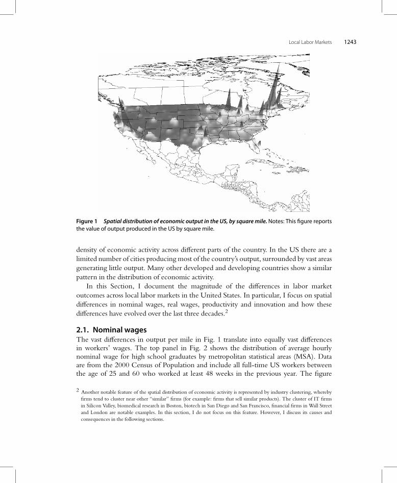
Most countries in the world are characterized by significant spatial heterogeneity ineconomic outcomes. As an example, Fig. 1 shows the amount of income producedby square mile in the United States. The map documents enormous differences in the
Local Labor Markets 1243
Figure 1 Spatial distribution of economic output in the US, by squaremile.Notes: This figure reportsthe value of output produced in the US by square mile.
density of economic activity across different parts of the country. In the US there are alimited number of cities producing most of the country’s output, surrounded by vast areasgenerating little output. Many other developed and developing countries show a similarpattern in the distribution of economic activity.
In this Section, I document the magnitude of the differences in labor marketoutcomes across local labor markets in the United States. In particular, I focus on spatialdifferences in nominal wages, real wages, productivity and innovation and how thesedifferences have evolved over the last three decades.2
2.1. Nominal wagesThe vast differences in output per mile in Fig. 1 translate into equally vast differencesin workers’ wages. The top panel in Fig. 2 shows the distribution of average hourlynominal wage for high school graduates by metropolitan statistical areas (MSA). Dataare from the 2000 Census of Population and include all full-time US workers betweenthe age of 25 and 60 who worked at least 48 weeks in the previous year. The figure
2 Another notable feature of the spatial distribution of economic activity is represented by industry clustering, wherebyfirms tend to cluster near other “similar” firms (for example: firms that sell similar products). The cluster of IT firmsin Silicon Valley, biomedical research in Boston, biotech in San Diego and San Francisco, financial firms in Wall Streetand London are notable examples. In this section, I do not focus on this feature. However, I discuss its causes andconsequences in the following sections.

1244 Enrico Moretti
Average wage of high school graduates in 2000
Average wage of college graduates in 2000
Figure 2 Distribution of average hourly nominal wage of high school graduates and collegegraduates, bymetropolitan area.Notes: This figure reports the distribution of average hourly nominalwage of high school graduates and for college graduates acrossmetropolitan areas in the 2000 Censusof Population. There are 288 metropolitan areas. The sample includes all full-time US born workersbetween the age of 25 and 60 who worked at least 48 weeks in the previous year.
indicates that labor costs vary significantly across US metropolitan areas. The averagehigh school graduate living in the median metropolitan area earns $14.1 for each hourworked. The 10th and 90th percentile of the distribution across metropolitan areas are$12.5 and $16.5, respectively. This amounts to a 32% difference in labor costs. The 1stand 99th percentile are $11.9 and $19.0, respectively, which amounts to a 60% difference.While some of these differences may reflect heterogeneity in skill levels within educationgroup, differences across metropolitan areas conditional on race, experience, gender, andHispanic origin are equally large.

Local Labor Markets 1245
Table 1 Metropolitan areas with the highest and lowest hourly wage of high school graduates in2000.Metropolitan area Averagehourlywage
Metropolitan areas with the highest wage
Stamford, CT 20.21San Jose, CA 19.70Danbury, CT 19.13San Francisco-Oakland-Vallejo, CA 18.97New York-Northeastern NJ 18.86Monmouth-Ocean, NJ 18.30Santa Cruz, CA 18.24Santa Rosa-Petaluma, CA 18.23Ventura-Oxnard-Simi Valley, CA 17.72Seattle-Everett, WA 17.71
Metropolitan areas with the lowest wage
Ocala, FL 12.12Dothan, AL 12.11Amarillo, TX 12.10Danville, VA 12.08Jacksonville, NC 12.02Kileen-Temple, TX 11.98El Paso, TX 11.96Abilene, TX 11.87Brownsville-Harlingen-San Benito, TX 11.23McAllen-Edinburg-Pharr-Mission, TX 10.65
The sample includes all full-time US born workers between the age of 25 and 60 with a high school degree who workedat least 48 weeks in the previous year. Data are from the 2000 Census of Population.
The bottom panel in Fig. 2 shows the distribution of average hourly nominal wagefor college graduates across metropolitan areas. (Note that the scale in the two panels isdifferent.) The distribution of the average wage of college graduates across metropolitanareas is even wider than the distribution of the average wage of high school graduates. The10th and 90th percentile of the distribution for college graduates are $20.5 and $28.5.This amounts to a 41% difference in labor costs. The 1st and 99th percentile are $18.1and $38.5, respectively, which amounts to a 112% difference.
Table 1 lists the 10 metropolitan areas with the highest average wage for high schoolgraduates and the 10 metropolitan areas with the lowest average wage for high schoolgraduates. High school graduates living in Stamford, CT or San Jose, CA earn an hourlywage that is two times as large as workers living in Brownsville, TX or McAllen, TXwith the same level of schooling. This difference remains effectively unchanged afteraccounting for differences in workers’ observable characteristics. Table 2 produces asimilar list for college graduates. The difference between wages in cities at the top ofthe distributions and cities at the bottom of the distribution is more pronounced for

1246 Enrico Moretti
Table 2 Metropolitan areas with the highest and lowest hourly wage of college graduates in 2000.
Metropolitan area Averagehourlywage
Metropolitan areas with the highest wage
Stamford, CT 52.46Danbury, CT 40.81Bridgeport, CT 38.82San Jose, CA 38.49New York-Northeastern NJ 36.03Trenton, NJ 35.52San Francisco-Oakland-Vallejo, CA 34.89Monmouth-Ocean, NJ 33.70Los Angeles-Long Beach, CA 33.37Ventura-Oxnard-Simi Valley, CA 33.07
Metropolitan areas with the lowest wage
Pueblo, CO 20.16Goldsboro, NC 20.15St. Joseph, MO 20.01Wichita Falls, TX 19.74Abilene, TX 19.70Sumter, SC 19.57Sharon, PA 19.52Waterloo-Cedar Falls, IA 18.99Altoona, PA 18.68Jacksonville, NC 18.21
The sample includes all full-time US born workers between the age of 25 and 60 with a college degree who worked atleast 48 weeks in the previous year. Data are from the 2000 Census of Population.
college graduates. The average hourly wage of college graduates in Stamford, CT isalmost three times larger than the hourly wage of college graduates in Jacksonville, NC.
This difference is robust to controlling for worker characteristics.The wage differences documented in Fig. 2 are persistent over long periods of time.
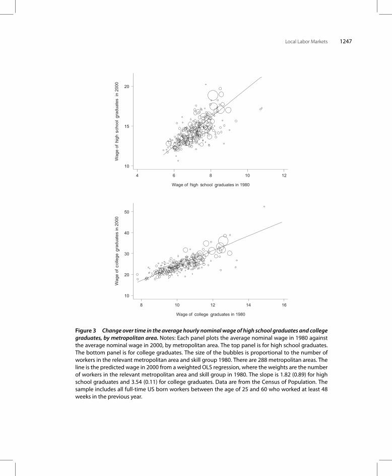
While in the decades after World War II regional differences in income were declining(Barro and Sala-i-Martin, 1991), convergence has slowed down significantly in morerecent decades. This can be seen in Fig. 3, where I plot the average hourly wage in 1980against the average wage in 2000 for high school graduates and college graduates, bymetropolitan area. The size of the bubbles is proportional to the number of workers inthe relevant metropolitan area and skill group 1980. The lines are the predicted wages in2000 from a weighted OLS regression, where the weights are the number of workers inthe relevant metropolitan area and skill group in 1980.
The figure suggests that there has been no mean reversion in wages since 1980. Infact, the opposite has happened. Wage differences across metropolitan areas have increasedover time. The slope of the regression line is 1.82 (0.89) for high school graduates. This
Local Labor Markets 1247
Figure 3 Change over time in the average hourly nominalwage of high school graduates and collegegraduates, by metropolitan area. Notes: Each panel plots the average nominal wage in 1980 againstthe average nominal wage in 2000, by metropolitan area. The top panel is for high school graduates.The bottom panel is for college graduates. The size of the bubbles is proportional to the number ofworkers in the relevant metropolitan area and skill group 1980. There are 288 metropolitan areas. Theline is the predicted wage in 2000 from a weighted OLS regression, where the weights are the numberof workers in the relevant metropolitan area and skill group in 1980. The slope is 1.82 (0.89) for highschool graduates and 3.54 (0.11) for college graduates. Data are from the Census of Population. Thesample includes all full-time US born workers between the age of 25 and 60 who worked at least 48weeks in the previous year.

1248 Enrico Moretti
Table 3 Average hourly wage in 1980 and 2000, by education level and metropolitan area.
High school graduates
Low wage in 2000 High wage in 2000Low wage in 1980 106 40High wage in 1980 34 108
College graduates
Low wage in 2000 High wage in 2000Low wage in 1980 114 32High wage in 1980 26 116
For each skill group, metropolitan areas are classified as having a low or high wage depending on whether their averagewage is below or above the average wage of the median metropolitan area in the relevant year. The sample includes allfull-time US born workers between the age of 25 and 60 who worked at least 48 weeks in the previous year. Data are fromthe 2000 Census of Population. There are 288 metropolitan areas.
suggests that metropolitan area where high school graduates have high wages in 1980compared to other metropolitan areas have even higher wages in 2000. The slope forcollege graduates is 3.54 (0.11). The fact that the slope is even higher for college graduatesindicates that the increase in the spatial differences in hourly wages is larger for skilledworkers.
The lack of spatial convergence is also documented in Table 3, where I classifymetropolitan areas as having low or high wage depending on whether the average wageis below or above the average wage in the median metropolitan area in the relevant year.This is done separately for each year and each education group. The top panel shows thatin most cases, metropolitan areas where high school graduates have high wages in 1980also have high wages in 2000. Only a quarter of metropolitan areas change category.Consistent with the larger increase in spatial divergence uncovered in Fig. 3, this fractionis even smaller for college graduates (bottom panel).
Using data on total income instead of hourly wages, Glaeser and Gottlieb (2009)find no evidence of convergenece across metropolitan areas between 1980 and 1990,
but they find some evidence of convergence between 1990 and 2000. The differencebetween their findings and Fig. 3 is explained by three factors. First, I am interestedin labor market outcomes, so that my sample includes only workers. By contrast, theGlaeser and Gottlieb sample includes all individuals. Second, there may be differencesacross metropolitan areas in unearned income. Third, and most importantly, there mightbe differences across metropolitan areas in number of hours worked, since it is wellknown that, since 1980, workers with high nominal wages have experienced relativelylarger increases in number of hours worked than workers with low nominal wages. Theconvergence in total income uncovered by Glaeser and Gottlieb (2009) in the 1990s isquantitatively limited. Consistent with my interpretation of Fig. 3, they conclude that

Local Labor Markets 1249
although there has been some convergence in income, over the last three decades “richplaces have stayed rich and poor places have stayed poor”.
When thinking about localization of economic activity, nominal wages are moreimportant than income because they are related to labor productivity. Since labor, capitaland goods can move freely within a country, it is difficult for an economy in a long-run equilibrium to maintain significant spatial differences in nominal labor costs in theabsence of equally large productivity differences. Indeed, if labor markets are perfectlycompetitive, nominal wage differences across local labor markets should exactly reflectdifferences in the marginal product of labor in industries that produce tradable goods. Ifthis were not the case, firms in the tradable sector located in cities with nominal wageshigher than labor productivity would relocate to less expensive localities. While not allworkers are employed in the tradable sector, as long as there are some firms producingtraded goods in every city and workers can move between the tradable and non-tradablesector, average productivity has to be higher in cities where nominal wages are higher.
Overall, if wages are related to marginal product of labor, there appears to be littleevidence of convergence in labor productivity across US metropolitan areas. If anything,there is evidence of divergence: metropolitan areas that are characterized by high laborproductivity in 1980 are characterized by even higher productivity in 2000. Notably,both the magnitude of geographic differences and speed of divergence appear to be morepronounced for high-skilled workers than low-skilled workers.
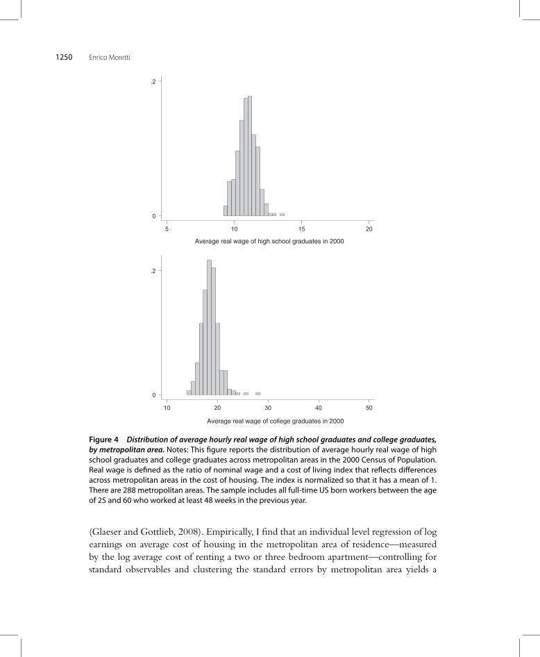
2.2. Real wagesThe large differences in nominal wages documented above do not appear to be associatedwith massive migratory flows of workers across metropolitan areas.3 The main reason forthe lack of significant spatial reallocation of labor is that land prices vary significantlyacross locations so that differences in real wages are significantly smaller than differencesin nominal wages. Figure 4 shows the distribution of average hourly real wage for highschool and college graduates across metropolitan areas. Real wages are calculated as theratio of nominal wages and a local CPI that reflects differences in the cost of housingacross locations. The index is described in detail in Moretti (forthcoming). A comparisonwith Fig. 2 indicates that the distribution of real wages is significantly more compressedthan the distribution of nominal wages. For example, the 10th and 90th percentile of thedistribution for high school graduates are $10.0 and $11.7. This is only a 17% difference.The 10th and 90th percentile of the distribution for college graduates are $16.7 and$20.4, a 22% difference.
If nominal wages adjust fully to reflect cost of living differences, and if amenitydifferences are not too important, a regression of log nominal wage on log cost of housingshould yield a coefficient approximately equal to the share of income spent on housing
3 In a recent review of the evidence, Glaeser and Gottlieb (2008) conclude that “there has been little tendency for peopleto move to high income areas”.
1250 Enrico Moretti
Average real wage of high school graduates in 2000
Average real wage of college graduates in 2000
Figure 4 Distribution of average hourly real wage of high school graduates and college graduates,by metropolitan area. Notes: This figure reports the distribution of average hourly real wage of highschool graduates and college graduates across metropolitan areas in the 2000 Census of Population.Real wage is defined as the ratio of nominal wage and a cost of living index that reflects differencesacross metropolitan areas in the cost of housing. The index is normalized so that it has a mean of 1.There are 288 metropolitan areas. The sample includes all full-time US born workers between the ageof 25 and 60 who worked at least 48 weeks in the previous year.
(Glaeser and Gottlieb, 2008). Empirically, I find that an individual level regression of logearnings on average cost of housing in the metropolitan area of residence—measuredby the log average cost of renting a two or three bedroom apartment—controlling forstandard observables and clustering the standard errors by metropolitan area yields a

Local Labor Markets 1251
Figure 5 Distribution of total factor productivity in manufacturing establishments, by county.Notes: This figure reports the distribution of average total factor productivity of manufacturingestablishments in 1992, by county. County-level TFP estimates are obtained from estimates ofestablishment level production functionsbasedondata from theCensus ofManufacturers. Specifically,they are obtained from a regression of log output on hours worked by blue and white collar workers,book value of building capital, book value of machinery capital, materials, industry and county fixedeffects. The figure shows the distribution of the coefficients on the county dummies. Regressions areweightedbyplant output. The sample is restricted to counties that had 10 ormore plants in either 1977or 1992 in the 2xxx or 3xxx SIC codes. There are 2126 counties that satisfy the sample restriction. Forconfidentiality reasons, any data from counties whose output was too concentrated in a small numberof plants are not in the figure (although they are included in the regression).
coefficient equal to 0.513 (0.024).4 Given that the share of income spent on housingis about 41% in 2000, this regression lends credibility to the notion that nominal wagesadjust to take into account differences in the cost of living across localities.
2.3. ProductivityThe vast differences in nominal wages across local labor markets reflect, at least in part,differences in productivity. Productivity is notoriously difficult to measure directly. Oneempirical measure of productivity at the establishment level is total factor productivity(TFP), defined as output after controlling for inputs.
Figure 5 shows the distribution of average total factor productivity of manufacturingestablishments in 1992 by county. County-level TFP estimates are obtained fromestimates of production functions based on data from the Census of Manufacturers.Specifically, they are obtained from a regression of log output on hours worked by blue
4 Data are from the 2000 Census of Population.
1252 Enrico Moretti
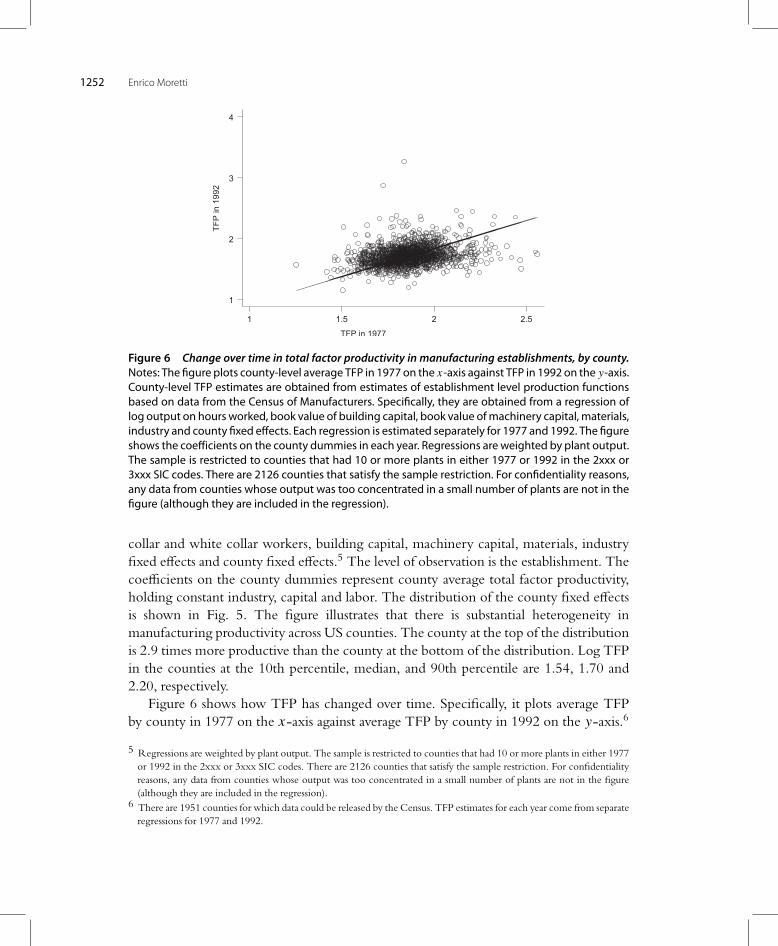
Figure 6 Change over time in total factor productivity in manufacturing establishments, by county.Notes: The figure plots county-level average TFP in 1977 on the x-axis against TFP in 1992 on the y-axis.County-level TFP estimates are obtained from estimates of establishment level production functionsbased on data from the Census of Manufacturers. Specifically, they are obtained from a regression oflog output on hours worked, book value of building capital, book value ofmachinery capital, materials,industry and county fixed effects. Each regression is estimated separately for 1977 and 1992. The figureshows the coefficients on the county dummies in each year. Regressions are weighted by plant output.The sample is restricted to counties that had 10 or more plants in either 1977 or 1992 in the 2xxx or3xxx SIC codes. There are 2126 counties that satisfy the sample restriction. For confidentiality reasons,any data from counties whose output was too concentrated in a small number of plants are not in thefigure (although they are included in the regression).
collar and white collar workers, building capital, machinery capital, materials, industryfixed effects and county fixed effects.5 The level of observation is the establishment. Thecoefficients on the county dummies represent county average total factor productivity,holding constant industry, capital and labor. The distribution of the county fixed effectsis shown in Fig. 5. The figure illustrates that there is substantial heterogeneity inmanufacturing productivity across US counties. The county at the top of the distributionis 2.9 times more productive than the county at the bottom of the distribution. Log TFPin the counties at the 10th percentile, median, and 90th percentile are 1.54, 1.70 and2.20, respectively.
Figure 6 shows how TFP has changed over time. Specifically, it plots average TFPby county in 1977 on the x-axis against average TFP by county in 1992 on the y-axis.6
5 Regressions are weighted by plant output. The sample is restricted to counties that had 10 or more plants in either 1977or 1992 in the 2xxx or 3xxx SIC codes. There are 2126 counties that satisfy the sample restriction. For confidentialityreasons, any data from counties whose output was too concentrated in a small number of plants are not in the figure(although they are included in the regression).
6 There are 1951 counties for which data could be released by the Census. TFP estimates for each year come from separateregressions for 1977 and 1992.
Local Labor Markets 1253
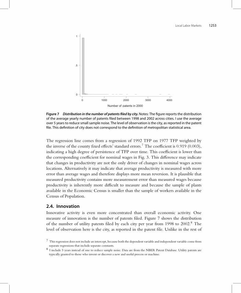
Figure 7 Distribution in the number of patents filed by city.Notes: The figure reports the distributionof the average yearly number of patents filed between 1998 and 2002 across cities. I use the averageover 5 years to reduce small sample noise. The level of observation is the city, as reported in the patentfile. This definition of city does not correspond to the definition of metropolitan statistical area.
The regression line comes from a regression of 1992 TFP on 1977 TFP weighted bythe inverse of the county fixed effects’ standard errors.7 The coefficient is 0.919 (0.003),indicating a high degree of persistence of TFP over time. This coefficient is lower thanthe corresponding coefficient for nominal wages in Fig. 3. This difference may indicatethat changes in productivity are not the only driver of changes in nominal wages acrosslocations. Alternatively it may indicate that average productivity is measured with moreerror than average wages and therefore displays more mean reversion. It is plausible thatmeasured productivity contains more measurement error than measured wages becauseproductivity is inherently more difficult to measure and because the sample of plantsavailable in the Economic Census is smaller than the sample of workers available in theCensus of Population.
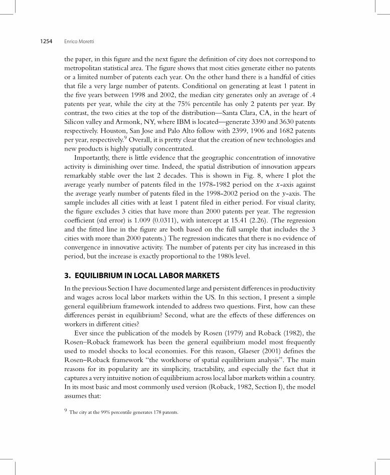
2.4. InnovationInnovative activity is even more concentrated than overall economic activity. Onemeasure of innovation is the number of patents filed. Figure 7 shows the distributionof the number of utility patents filed by each city per year from 1998 to 2002.8 Thelevel of observation here is the city, as reported in the patent file. Unlike in the rest of
7 This regression does not include an intercept, because both the dependent variable and independent variable come fromseparate regressions that include separate constants.
8 I include 5 years instead of one to reduce sample noise. Data are from the NBER Patent Database. Utility patents aretypically granted to those who invent or discover a new and useful process or machine.
1254 Enrico Moretti
the paper, in this figure and the next figure the definition of city does not correspond tometropolitan statistical area. The figure shows that most cities generate either no patentsor a limited number of patents each year. On the other hand there is a handful of citiesthat file a very large number of patents. Conditional on generating at least 1 patent inthe five years between 1998 and 2002, the median city generates only an average of .4patents per year, while the city at the 75% percentile has only 2 patents per year. Bycontrast, the two cities at the top of the distribution—Santa Clara, CA, in the heart ofSilicon valley and Armonk, NY, where IBM is located—generate 3390 and 3630 patentsrespectively. Houston, San Jose and Palo Alto follow with 2399, 1906 and 1682 patentsper year, respectively.9 Overall, it is pretty clear that the creation of new technologies andnew products is highly spatially concentrated.
Importantly, there is little evidence that the geographic concentration of innovativeactivity is diminishing over time. Indeed, the spatial distribution of innovation appearsremarkably stable over the last 2 decades. This is shown in Fig. 8, where I plot theaverage yearly number of patents filed in the 1978-1982 period on the x-axis againstthe average yearly number of patents filed in the 1998-2002 period on the y-axis. Thesample includes all cities with at least 1 patent filed in either period. For visual clarity,the figure excludes 3 cities that have more than 2000 patents per year. The regressioncoefficient (std error) is 1.009 (0.0311), with intercept at 15.41 (2.26). (The regressionand the fitted line in the figure are both based on the full sample that includes the 3cities with more than 2000 patents.) The regression indicates that there is no evidence ofconvergence in innovative activity. The number of patents per city has increased in thisperiod, but the increase is exactly proportional to the 1980s level.
3. EQUILIBRIUM IN LOCAL LABORMARKETSIn the previous Section I have documented large and persistent differences in productivityand wages across local labor markets within the US. In this section, I present a simplegeneral equilibrium framework intended to address two questions. First, how can thesedifferences persist in equilibrium? Second, what are the effects of these differences onworkers in different cities?
Ever since the publication of the models by Rosen (1979) and Roback (1982), theRosen–Roback framework has been the general equilibrium model most frequentlyused to model shocks to local economies. For this reason, Glaeser (2001) defines theRosen–Roback framework “the workhorse of spatial equilibrium analysis”. The mainreasons for its popularity are its simplicity, tractability, and especially the fact that itcaptures a very intuitive notion of equilibrium across local labor markets within a country.In its most basic and most commonly used version (Roback, 1982, Section I), the modelassumes that:
9 The city at the 99% percentile generates 178 patents.

Local Labor Markets 1255
Figure 8 Change over time in the number of patents filed by city. Notes: The x-axis is the averageyearly number of patents filed between 1978 and 1982. The y-axis is the average yearly number ofpatents filed between 1998 and 2002. I use the averages over 5 years to reduce sample noise. The levelof observation is the city, as reported in the patent file. This definition of city does not correspond tometropolitan statistical area. For visual clarity, the figure excludes 3 cities that have more than 2000patents per year. A regression based on the full sample (i.e. including the cities with more than 3000patents per year) yields a coefficient (std error) equal to 1.009 (0.0311). The fitted line in the figure isbased on the full sample (i.e. including the 3 cities with more than 2000 patents per year).
1. Each city is a competitive economy that produces a single internationally traded goodusing labor, land and a local amenity. Technology has constant returns to scale
2. Workers’ indirect utility depends on nominal wages, cost of housing and localamenities
3. Labor is homogenous in skills and tastes10 and each worker provides one unit of labor4. Labor is perfectly mobile so that the local labor supply is infinitely elastic5. Land is the only immobile factor and its supply is fixed.
In its simplest form, and the one that is most commonly used in the literature(Roback, 1982, Section I), the Rosen–Roback key insight is that any local shock to thedemand or supply of labor in a city is, in equilibrium, fully capitalized in the price of land.As a consequence, shocks to a local economy do not affect worker welfare. Consider, forexample, a productivity shock that makes workers in city c more productive than workersin other cities. In the Rosen–Roback framework, the increase in productivity in city cresults in an increase in nominal wages in city c and a similar increase in housing costs incity c, so that in equilibrium workers are completely indifferent between city c and all theother cities. In the new equilibrium, workers are more productive but they are not better
10 Roback (1988) considers the cases of heterogenous labor.
1256 Enrico Moretti
off. The owners of land in city c are better off, by an amount equal to the productivityincrease. This result depends on the assumption that the local labor supply is infinitelyelastic and that the elasticity of housing supply is limited.11
The assumptions of this model are restrictive, and rule out some interesting questionsregarding the incidence of localized shocks to a local economy. In this section, I presenta more general equilibrium framework that seeks to take the spatial equilibrium model astep closer to reality. The goal of the model is to clarify what happens to wages, costs ofhousing and worker utility when a local economy experiences a shock to labor demandor labor supply. An example of a shock to labor demand is an increase in productivity.An example of a shock to labor supply is an increase in amenities. I assume that workersand firms are mobile across cities, but worker mobility is not necessarily infinite, becauseworkers have idiosyncratic preferences for certain locations. Moreover, housing supply isnot necessarily fixed. This implies that the elasticity of local labor supply is not necessarilyinfinite and the elasticity of housing supply is not necessarily zero. In this context,shocks to a local economy are not necessarily fully capitalized into land prices. This isimportant, because it allows for interesting distributional and welfare implications. Themodel clarifies exactly how the welfare consequences of localized labor market shocksdepend on the relative magnitude of the elasticities of local labor supply and housingsupply.
In Section 3.1 I describe the case of homogenous labor. It is a useful and transparentstarting point. It clarifies the role that the elasticity of labor and housing supply play indetermining how shocks to a local economy affect workers’ utility. In reality, however,workers are not all homogenous but they differ along many dimensions, most notably intheir skill level. Moreover, shocks to local economies rarely affect all workers equally.Instead, shocks to local economies are often skill-biased in the sense that they shiftthe demand for some skill groups more than others. For these reasons, in Section 3.2I describe the more general case of heterogenous labor. In Section 3.3 I allow foragglomeration economies. In Section 3.4 I discuss the case where there are multipleindustries within each local economy and local multipliers. In Section 3.5 I review someof the existing empirical evidence.
11 In the simplest form of the model, there is one margin of adjustment that allows to accommodate some in-migrationto the more productive city. While land is assumed to be fixed, workers can adjust their consumption of housing.
When housing prices increase in city c, each worker consumes a little less housing. This allows a small increase inthe number of workers in the more productive city, even with fixed land. In a more general version of the model,Roback (1982, Section II) keeps the assumption that land is fixed but allows for the production of housing. Housingproduction is assumed to use labor, which is perfectly mobile, and land, which is fixed. In this version of the model,there are two margins of adjustment that allow to accommodate in-migration to a city. First, like before, workers canadjust their consumption of housing in response to increases in housing prices. Second, unlike before, the housingstock can increase in response to increased demand. In this version of the model, more workers change city after acity-specific productivity shock. However, the key implication for incidence of the shock does not change. Becauseworkers are assumed to be perfectly mobile and homogenous, their utility is never affected by the shock.
Local Labor Markets 1257
Over the years, many versions of the spatial equilibrium model have been proposed.The version of model that I present is based on Moretti (forthcoming). The proposedframework is based on assumptions designed to make it very simple and transparent whileat the same time not unrealistic. The model seeks to describe spatial equilibrium in thelong run and is probably not well suited to describe year to year adjustments.12 Topel(1986) and Glaeser (2008) propose alternative equilibrium frameworks that take intoaccount the dynamics of wages and employment. Roback (1982), Glaeser (2008) andGlaeser and Gottlieb (2009) propose frameworks where housing production uses bothlocal labor (and of course land). By contrast, in my simplified framework housingproduction does not use local labor. Combes et al. (2005) link the spatial equilibriumframework to some of the insights from the New Economic Geography literature.
3.1. Spatial equilibriumwith homogeneous labor3.1.1. Assumptions and equilibriumI begin by considering the case where there is only one type of labor. As in Rosen–Roback, I assume that each city is a competitive economy that produces a single outputgood y which is traded on the international market, so that its price is the sameeverywhere and set equal to 1. Workers and firms are mobile and locate where utilityand profits are maximized. Like in Roback, I abstract from labor supply decisions andI assume that each worker provides one unit of labor, so that local labor supply is onlydetermined by workers’ location decisions. The indirect utility of worker i in city c is
Uic = wc − rc + Ac + eic (1)
where wc is the nominal wage in city c; rc is the cost of housing; Ac is a measure oflocal amenities.13 The random term eic represents worker i idiosyncratic preferences forlocation c. A larger eic means that worker i is particularly attached to city c, holdingconstant real wage and amenities. For example, being born in city c or having family incity c may make city c more attractive to a worker irrespective of city c’s real wages andamenities. Assume that there are two cities: city a and city b and that worker i ’s relativepreference for city a over city b is
eia − eib ∼ U [−s, s]. (2)
The parameter s characterizes the importance of idiosyncratic preferences forlocation and therefore the degree of labor mobility. If s is large, it means that preferencesfor location are important and therefore worker willingness to move to arbitrage awayreal wage differences or amenity differences is limited. On the other hand, if s is small,
12 The reason is that in the short run, frictions in labor mobility and in housing supply may constrain the ability of workersand housing stock to fully adjust to shocks.
13 In Roback’s terminology, Ac is a consumption amenity.

1258 Enrico Moretti
preferences for location are not very important and therefore workers are more willing tomove in response to differences in real wages or amenities. In the extreme, if s = 0 thereare no idiosyncratic preferences for location and therefore worker mobility is perfect.
While parsimonious, the model captures the four most important factors that mightdrive worker mobility: wages, the cost of living, amenities, and individual preferences.A worker chooses city a if and only if eia − eib > (wb − rb) − (wa − ra) + (Ab −
Aa). In equilibrium, the marginal worker needs to be indifferent between cities. Thisequilibrium condition implies that local labor supply is upward sloping, and its slopedepends on s. For example, local labor supply in city b is
wb = wa + (rb − ra)+ (Aa − Ab)+ s(Nb − Na)
N(3)
where Nc is the endogenously determined log of number of workers in city c; andN = Na + Nb is assumed fixed. The key point of Eq. (3) is that the elasticity of locallabor supply depends on worker preferences for location. If idiosyncratic preferences forlocation are very important (s is large), then workers are relatively less mobile and theelasticity of local labor supply is low. In this case, the local labor supply curve is relativelysteep. If idiosyncratic preferences for location are not very important (s is small), thenworkers are relatively more mobile and the elasticity of local labor supply is high. In thiscase, the local labor supply curve is relatively flat. In the case of perfect mobility (s = 0),the elasticity of local labor supply is infinite and the local labor supply curve is perfectlyflat. In that case, any difference in real wages or in amenities, however small, results in aninfinitely large number of workers willing to leave one city for the other.14 The interceptin Eq. (3) indicates that, for a given slope, if the real wage in city a increases or localamenities improve, workers leave city b and move to city a.
An important difference between the Rosen–Roback setting and this setting is thatin Rosen–Roback, all workers are identical, and always indifferent across locations. Inthis setting, workers differ in their preferences for location. While the marginal worker isindifferent between locations, here there are inframarginal workers who enjoy economicrents. These rents are larger the smaller the elasticity of local labor supply.15
14 Tabuchi and Thisse (2002) model how worker heterogeneity generates an upward sloping local labor supply and howthis affects the spatial distribution of economic activity.
15 It is not easy to obtain credible empirical estimates of the elasticity of local labor supply. First, one needs to isolatelabor market shocks that are both localized and demand driven. Second, one needs to identify the effect both onwages and land prices. For example, Greenstone et al. (forthcoming) document that the exogenous opening of a largemanufacturing establishment in a county is associated with a significant increase in employment and local nominalwages. The wage increase appears to persist five years after the opening of the new plant. However, this result per sedoes not necessarily imply that local labor supply is upward sloping. As Eq. (3) indicates, what matters in this respectis whether the demand-driven shift in employment causes wages to increase over and above land costs. The findingthat an increase in the local demand for labor results in an increase in local wages does not per se imply that local laborsupply is upward sloping. In principle, such finding is consistent with a spatial equilibrium where the local supply oflabor is infinitely elastic but the supply of housing is inelastic.
Local Labor Markets 1259
The production function for firms in city c is Cobb–Douglas with constant returnsto scale, so that
ln yc = Xc + hNc + (1− h)Kc (4)
where Xc is a city-specific productivity shifter;16 and Kc is the log of capital. I focus firston the case where Xc is given. Later, I discuss the model with agglomeration economiesin which Xc is a function of density of economic activity or human capital. Firms areassumed to be perfectly mobile. If firms are price takers and labor is paid its marginalproduct, labor demand in city c is
wc = Xc − (1− h)Nc + (1− h)Kc + ln h. (5)
I assume that there is an international capital market, and that capital is infinitelysupplied at a given price i .17 I also assume that each worker consumes one unit ofhousing. This implies that the (inverse of) the local demand for housing is just a re-arrangement of Eq. (3):
rb = (wb − wa)+ ra + (Ab − Aa)− s(Nb − Na)
N. (6)
To close the model, I assume that the supply of housing is
rc = z + kc Nc (7)
where the number of housing units in city c is assumed to be equal to the number ofworkers. The parameter kc characterizes the elasticity of the supply of housing. I assumethat this parameter is exogenously determined by geography and local land regulations. Incities where geography and regulations make it is easy to build new housing, kc is small.In the extreme case where there are no constraints to building new houses, the supplycurve is horizontal, and kc is zero. In cities where geography and regulations make itdifficult to build new housing, kc is large. In the extreme case where it is impossible tobuild new houses, the supply curve is vertical, and kc is infinite. A limitation of Eq. (7)is that it implicitly makes two assumptions that, while helpful in simplifying the model,are not particularly realistic. First, housing production in this model does not involve theuse of any local input. Roback (1982) and Glaeser (2008), among others, discuss spatialequilibrium in the case where housing production involves the use of local labor andother local inputs. Second, Eq. (7) ignores the durability of housing. Glaeser (2008) pointout that once built, the housing stock does not depreciate quickly and this introduces an
16 In Roback terminology, Xc is a productive amenity.17 In equilibrium, the marginal product of capital has to be equal to Xc − hKc + hNc + ln(1− h) = ln i .
1260 Enrico Moretti
asymmetry between positive and negative demand shocks. In particular, when demanddeclines, the quantity of housing cannot decline, at least in the short run. The possibleimplications of this asymmetry are analyzed by Notowidigdo (2010).
Equilibrium in the labor market is obtained by equating Eqs (3) and (5) for each city.Equilibrium in the housing market is obtained by equating Eqs (6) and (7).
In this framework, workers and landowners are separate agents and landowners areassumed to live abroad. While in reality most workers own their residence, keepingworkers separate from landowners has the advantage of allowing me to separately identifythe welfare consequences of changes in housing values from the welfare consequences ofchanges in labor income. This is important both for conceptual clarity and for thinkingabout the different implications of the results for labor and housing policies.18
This model differs from the model of local labor markets proposed by Topel (1986)because it ignores dynamics. This model also differs from most of the existing versions ofthe spatial equilibrium model in that it describes a closed economy with a fixed numberof workers, so that shock to a given city affects the other city. For example, an increase inlabor demand in city b affects labor supply, wages and prices in city a. By contrast, mostexisting versions of the spatial equilibrium model assume that local shocks to a city affectlocal outcomes there, but have a negligible effect on the rest of the national economybecause the rest of the economy is large relative to the city. (See for example: Glaeser(2008, 2001) and Notowidigdo (2010)). In this sense most of the existing models are nottruly general equilibrium models.19
3.1.2. Effect of a labor demand shock onwages and pricesI begin by considering the effect of an increase in labor demand in city b. This demandincrease could be due to a localized technological shock that increases the productivity offirms located in city b. Alternatively, it could be due to an improvement in the productdemand faced by firms in city b. Later, I consider the effect of an increase in labor supplyin city b.
I assume that in period 1, the two cities are identical and in period 2, total factorproductivity increases in city b. Specifically, I assume that in period 2, the productivityshifter in b is higher than in period 1: Xb2 = Xb1 + 1, where 1 > 0 represents a
18 On the other hand, this assumption has the disadvantage that it misses some important features of housing and labormarkets. When workers are also property owners, a localized increase in housing values in a city implies both an increasein the value of the asset but also an increase in the user cost of housing. The only way for property owners to access theincreased value of the asset is to move to a different city.
19 In the interest of simplicity, the model completely ignores congestions costs. Equilibrium is achieved only becausehousing costs in a city increase when population increases. In reality, congestion costs (for example: transportationcosts) are probably an another important determinant of equilibrium across cities. Allowing for congestion costs wouldnot alter the qualitative predictions of the model, but it would result in smaller predicted increases in housing costs incities that experience positive productivity shocks. The reason is simple. As a city becomes more productive and itsworkforce increases, commuting costs increase, thus reducing its relative attractiveness.
Local Labor Markets 1261
positive, localized, unexpected productivity shock.20 I have added subscripts 1 and 2 todenote periods 1 and 2. The amenities in the two cities are assumed to be identical andto remain unchanged.
Workers are now more productive in city b than a. Attracted by this higherproductivity, some workers move from a to b:
Nb2 − Nb1 =N
N (ka + kb)+ 2s1 ≥ 0. (8)
The equation indicates that number of movers is larger the elasticity of labor supply(i.e. the smaller is s) and the larger the elasticity of housing supply in city b (i.e. the smalleris kb). This is not surprising, because a smaller s implies that idiosyncratic preferences forlocation are less important, and therefore that labor is more mobile in response to realwage differentials. A smaller kb means that it is easier for city b to add new housing unitsto accommodate the increased demand generated by the in-migrants.
The nominal wage in city b increases by an amount equal to the productivity increase:
wb2 − wb1 = 1. (9)
Because of in-migration, the cost of housing in city b needs to increase. The magnitudeof the increase is a fraction of1 and depends on how elastic is housing supply in b relativeto a:
rb2 − rb1 =kb N
N (ka + kb)+ 2s1 ≥ 0. (10)
This increase in housing costs is larger the smaller the elasticity of housing supply in cityb (large kb) relative to city a. Because nominal wages increase more than housing costs(compare Eqs (9) and (10)), real wages increase in b:
(wb2 − wb1)− (rb2 − rb1) =ka N + 2s
N (ka + kb)+ 2s1 ≥ 0. (11)
Although the original productivity shock only involves city b, in general equilibrium,prices in city a are also affected. In particular, out-migration lowers the cost of housing.21
20 I am modeling the productivity shock as an increase in total factor productivity. Results are similar in the case wherethe shock only increases productivity of labor.
21 The change in the cost of housing in a is
ra2 − ra1 = −ka N
N (ka + kb)+ 2s1 ≤ 0. (12)

1262 Enrico Moretti
Because the nominal wage in a does not change,22 the net effect is an increase in realwages in a:
(wa2 − wa1)− (ra2 − ra1) =ka N
N (ka + kb)+ 2s1 ≥ 0. (13)
It is important to note that in general, real wages differ in the two cities in period 2.In particular, a comparison of Eq. (11) with Eq. (13) indicates that in period 2 real wagesare higher in city b. This is not surprising, because city b is the one directly affectedby the productivity shock. While labor mobility causes real wages to increase in city aas well, real wages are not fully equalized because mobility is not perfect in that onlythe marginal worker is indifferent between the two cities in equilibrium. With perfectmobility (s = 0), real wages are completely equalized because all workers need to beindifferent between the two cities.23
The marginal worker in period 2 is different from the marginal worker in period 1.Since city b offers higher real wages in period 2, the new marginal worker in period 2has stronger preferences for city a. In particular, the change in the relative preference forcity a of the marginal worker is equal to24
(ea2 − eb2)− (ea1 − eb1) =2s1
N (ka + kb)+ 2s≥ 0. (14)
Note that firms are indifferent between cities. Because of the assumptions ontechnology, firms have zero profits in both cities. While labor is now more expensivein b, it is also more productive there. Because firms produce a good that is internationallytraded, if skilled workers weren’t more productive, employers would leave b and relocateto a.
In the production function used here, all firms in a city are assumed to sharea city-specific productivity shifter. The implicit assumption is that any city-specificcharacteristic affects all firms equally. For example, the transportation infrastructure, theweather, local institutions, local regulations, etc. affect the productivity of all producersin the same way. It would be easy to extend this framework to allow for an additionalfirm-city specific productivity shifter:
ln y jc = (Xc + X jc)+ hN jc + (1− h)K jc (15)
22 This may look surprising at first. Given that the number of workers has declined, and that the demand curve isdownward sloping, one might expect an increase in wages of those workers who stay in a. Indeed, this would betrue in a model without capital. But in a model that includes capital, the amount of capital used by firms declines in band increases in a. This capital flow off-sets the changes in labor supply.
23 To see this, compare Eq. (11) with (13), setting s = 0.24 This change is by construction equal to the change in the difference in real wages between the two cities.

Local Labor Markets 1263
where j indexes a firm, Xc is a productivity effect shared by all firms in city c, andX jc is a productivity effect that is specific to firm j and city c. This formulation allowssome firms to benefit more from some city characteristics than others. For example, thespecific type of local infrastructure in a given city may affect the TFP of some firms morethan others. This is analogous to introducing individual specific location preferences inworkers’ utility functions. For the same reason that preferences for location make workersless responsive to differences in real wages across locations, the term X jc makes firms lessmobile. Effectively, some firms enjoy economic rents generated by their location-firmspecific match. Small differences in production costs may not be enough to induce thesefirms to relocate, in the same way that worker idiosyncratic preferences for location lowerthe elasticity of labor supply.
3.1.3. Incidence: who benefits from the productivity increase?In this setting, the benefit of the increase in productivity 1 is split between workers andlandowners.25 Eqs (10)–(13) clarify that the incidence of the shock depends on which ofthe two factors—labor or land—is supplied more elastically at the local level. In turn, theelasticity of local labor supply and the elasticity of housing supply ultimately depend onthe preference parameter s and the supply parameters ka and kb. For a given elasticity ofhousing supply, a lower local elasticity of labor supply implies that a larger fraction of theproductivity shock in city b accrues to workers in city b, and a smaller fraction accrues tolandowners in city b. Intuitively, when labor is relatively less mobile, it captures more ofthe economic rent generated by the productivity shock. A lower local elasticity of laborsupply also implies a smaller increase in real wages in the non affected city (city a), sincethe channel that generates benefits for the non affected city is the potential for workermobility.
On the other hand, for a given elasticity of labor supply, a lower elasticity of housingsupply in city b relative to city a (kb bigger than ka) implies that housing quantity adjustsless in city b following the productivity shock. As a consequence, housing prices increasemore and a larger fraction of the productivity gain accrues to landowners in city b and asmaller fraction accrues to workers.
The role played by the elasticity of labor and housing supply in determining theincidence of the productivity shock between workers and landowners and between citya and city b is clearly illustrated in four special cases.
1. If labor is completely immobile (s = ∞), Eq. (11) becomes (wb2 − wb1) − (rb2 −
rb1) = 1, indicating that real wages in city b increase by the full amount of theproductivity shock. In this case, the benefit of the shock accrues entirely to workers incity b. The intuition is that if labor is a fixed factor, workers in the city hit by the shock
25 By construction: 1 = change in real wage in a + change in real wage in b + change in land price in a + change inland price in b.

1264 Enrico Moretti
capture the full economic rent generated by the shock. Nothing happens to workersin a, as their real wage is unchanged: Eq. (13) becomes (wa2−wa1)−(ra2−ra1) = 0.Moreover, since no worker moves in equilibrium, housing prices in both citiesremain unchanged so that landowners are indifferent. For example, Eq. (10) becomesrb2 − rb1 = 0, indicating that housing prices in b are not affected.
2. If labor is perfectly mobile (s = 0), Eqs (11) and (13) become: (wb2 −wb1)− (rb2 −
rb1) = (wa2 − wa1) − (ra2 − ra1) =ka
ka+kb1. Because of perfect labor mobility,
real wages need to be identical in a and b, otherwise workers would leave one cityfor the other. In this case, incidence depends on the relative elasticities of housingsupply in the two cities. To see this, note that the increase in real wages is a fraction
kaka+kb
of 1. The rest of 1 accrues to landowners in b, since housing prices in b
increase by rb2 − rb1 =kb
ka+kb1. The fraction that accrues to workers depends on
which of the two cities has more elastic housing supply. For example, if the elasticityof housing supply is the same in a and b, than we have an equal split between workersand landowners, with real wages in both cities increasing by 1
21, and land prices inb increasing by 1
21. On the other hand, if the elasticity of housing supply is larger incity b then landowners capture less of the total economic rent, because their factor ismore elastically supplied in the city originally hit by the shock.
3. If housing supply in b is fixed (kb = ∞), the entire productivity increase is capitalizedin land values in city b. This is the Rosen–Roback case described above. City bbecomes more productive but it cannot expand its workforce because housing cannotexpand. No one can move to city b, and the only effect of the productivity shock isto raise cost of housing by rb2 − rb1 = 1. All the benefit goes to landowners in b.Real wages are not affected, and workers in both cities are indifferent. This is a casewhere, even in the presence of a shock that makes some firms more productive, laboris prevented from accessing this increased productivity by the constraints on housingsupply. Part of the increase in productivity is therefore wasted.
4. If housing supply in b is infinitely elastic (kb = 0), then Eq. (10) becomes rb2− rb1 =
0, indicating that housing prices in b do not change. For each additional worker whointends to move to city b, a housing unit is added so that housing prices never increase.Landowners are indifferent, and the entire benefit of the productivity increase accruesto workers. Equation (11) becomes (wb2 − wb1)− (rb2 − rb1) = 1, indicating thatreal wages in city b increase by the full amount of the productivity shock. Real wagesin city a also increase, but less than in b: (wa2 − wa1)− (ra2 − ra1) =
ka NNka+2s1.
3.1.4. Effect of a labor supply shock onwages and pricesSo far, I have focused on what happens to a local economy following a shock generatedby a labor demand shift. What distinguishes city b from city a, is that in city b the demandfor labor is higher. I now discuss the opposite case, where a local economy experiences anincrease in the supply of labor. Specifically, I consider what happens when city b becomes
Local Labor Markets 1265
more desirable for workers relative to city a. I assume that in period 2, the amenity levelincreases in city b: Ab2 = Ab1 + 1
′, where 1′ > 0 represents the improvement in theamenity. I assume that the amenity level in a does not change, and that productivity is thesame in the two cities.26
As in the case of a demand shift above, NN (ka+kb)+2s1
′ workers move from a to b.As before, the cost of housing increases in b (by the amount in Eq. (10)) and declines ina (by the amount in Eq. (12)). Also, similar to before, the nominal wage in a does notchange. A difference with the demand shock case is that the nominal wage in b does notincrease, but it remains unchanged.27
As a consequence, real wages decline in city b
(wb2 − wb1)− (rb2 − rb1) = −kb N
N (ka + kb)+ 2s1′ ≤ 0 (16)
and increase in city a:
(wa2 − wa1)− (ra2 − ra1) =ka N
N (ka + kb)+ 2s1′ ≥ 0. (17)
Intuitively, workers are willing to take a negative compensating differential in theform of lower real wages to live in the more desirable city. Landowners in b experiencean increase in their property values, while landowners in a experience a decline.
The incidence of the shock is similar to what I discuss in Section 3.1.3. As with thecase of a demand shock, the exact magnitude of workers’ and landowners’ gains andlosses depend on the elasticity of labor supply and the elasticity of housing supply. Thefour special cases outlined in Section 3.1.3 apply to this case as well.
3.2. Spatial equilibriumwith heterogenous laborIn Section 3.1, I have considered the case where all workers are identical in terms ofproductivity. In this section, I consider the case where there are 2 types of workers: skilledworkers (type H ) and unskilled workers (type L). I assume that skilled and unskilledworkers in the same city face the same housing market. I discuss what happens in
26 Here, the labor supply increase is a consequence of an increase in amenities, holding constant tastes. Results are similarif one assumes that amenities are fixed, but the taste for those amenities increases.
27 This may seem counterintuitive at first. One might expect wage decreases in response to supply increases. Why donominal wages not decline in b after it has become more attractive? After all, workers should be willing to take anegative compensating differential in the form of lower nominal wages to live in the more desirable city. Indeed, thisis what a model without capital would predict. However, such a model ignores the endogenous reaction of capital.In a model with capital, nominal wages do not move in city b because capital flows to b, offsetting the changes
in labor supply. The amount of capital increases in b by Kb2 − Kb1 =N1′
N (ka+kb)+2s ≥ 0 and decreases in a by
Ka2 − Ka1 = −N1′
N (ka+kb)+2s ≤ 0.

1266 Enrico Moretti
equilibrium when the demand for one group changes in one city, while the demandfor the other group remains unchanged.
3.2.1. Assumptions and equilibriumThe indirect utilities of skilled workers and unskilled workers in city c are assumed to be,respectively
UHic = wHc − rc + AHc + eHic (18)
and
ULic = wLc − rc + ALc + eLic. (19)
In Eqs (18) and (19), skilled and unskilled workers in a city face the same price of housingso that a shock to the labor demand of one group may be transmitted to the other groupthrough its effect on housing prices.28 While they have access to the same local amenities,different skill groups do not need to value these amenities equally: AHc and ALc representthe skill-specific value of local amenities. Tastes for location can vary by skill group.Specifically, I assume that skilled workers’ and unskilled workers’ relative preferences forcity a over city b are, respectively
eHia − eHib ∼ U [−sH , sH ] (20)
and
eLia − eLib ∼ U [−sL , sL ]. (21)
For example, the case in which skilled workers are more mobile than unskilled workerscan be modeled by assuming that sH < sL .
For simplicity, I focus on the case where skilled and unskilled workers in the same citywork in different firms. This amounts to assuming away imperfect substitution betweenskilled and unskilled workers. This assumption simplifies the analysis, and it is not crucial.The production function for firms in city c that use skilled labor is Cobb–Douglas withconstant returns to scale: ln yHc = X Hc+hNHc+ (1−h)K Hc, where K Hc is the log ofcapital and X Hc is a skill and city-specific productivity shifter. Similarly, the production
28 It is easy to relax this assumption by assuming residential segregation along skill lines within a city. However, thisassumption would not be particularly realistic. Although skilled and unskilled individuals may reside in different partsof a metropolitan area, there always is some overlap which ensures that shocks to a part of the metropolitan area gettransmitted to the rest of the area. Empirically, changes in housing prices across neighborhoods within a city are highlycorrelated.

Local Labor Markets 1267
function for firms that use unskilled labor is ln yLc = X Lc + hNLc + (1− h)KLc. Therest of the assumptions remain unchanged.29
3.2.2. Effect of a labor demand shock onwages and pricesConsider the case where the relative demand for skilled labor increases in b. See Moretti(forthcoming) for the specular case where the relative supply for skilled labor increasesin b.
Assume that the productivity of skilled workers increases relative to the productivityof unskilled workers in city b because the productivity shifter for skilled workers in cityb is higher in period 2 than in period 1: X Hb2 = X Hb1 +1, where 1 > 0 represents apositive, localized, skill-biased productivity shock. Nothing happens to the productivityof unskilled workers in b and the productivity of skilled and unskilled workers in a. Theamenities in the two cities are identical and fixed.
Attracted by higher labor demand, some skilled workers move to b from a. Inparticular, the number of skilled workers in b increases by
NHb2 − NHb1 =1N ((ka + kb)N + 2sL)
2h(ka N (sH + sL)+ kb N (sH + sL)+ 2sH sL)≥ 0. (23)
This number depends positively on the elasticity of labor supply for skilled and unskilledworkers:
∂(NHb2 − NHb1)
∂sH= −
N (ka N + 2sL + kb N )21
2h(ka NsH + 2sH sL + ka NsL + kb NsH + kb NsL)2≤ 0
(24)
and
∂(NHb2 − NHb1)
∂sL= −
N 31(2kakb + k2a + k2
b)
2h(ka NsH + 2sH sL + ka NsL + kb NsH + kb NsL)2≤ 0.
(25)
The intuition for the first derivative is obvious: a higher elasticity of labor supply forskilled workers implies that skilled workers are more mobile. The intuition for the second
29 Because skilled and unskilled workers face the same housing market within a city, to obtain the (inverse of) theaggregate demand curve for housing in a city one needs to sum the demand of skilled workers and the demand ofunskilled workers. For example,in city b:
rb =(2sH sL )
(sH + sL )−(2sH sL )(NHb + NLb)
N (sH + sL )−
sL (wHa − wHb − ra)
(sL + sH )−
sH (wLa − wLb − ra)
(sL + sH ). (22)

1268 Enrico Moretti
derivative is less obvious. A higher elasticity of labor supply for unskilled workers impliesthat a larger number of unskilled workers move out in response to the inflow of skilledworkers, so that the increase in housing costs is more limited which ultimately increasesthe number of skilled in-migrants.
The number of movers in Eq. (23) also depends positively on the elasticity of housingsupply in b:
∂(NHb2 − NHb1)
∂kb= −
N 21s2L
h(ka NsH + 2sH sL + ka NsL + kb NsH + kb NsL)2≤ 0.
(26)
A higher elasticity of housing supply (lower kb) implies that more housing units becomeavailable for the incoming skilled workers.
Because skilled workers in b have become more productive, their nominal wageincreases by an amount 1/h, proportional to the productivity increase. Following theinflow of skilled workers, the cost of housing in b increases and the increase is larger thesmaller is sH and the larger is kb:30
rb2 − rb1 =sL Nkb1
h(ka NsH + 2sH sL + ka NsL + kb NsH + kb NsL)≥ 0. (27)
Skilled workers in both cities experience increases in real wages. In b, the increase inreal wages is smaller than the increase in nominal wages because of the increase in thecost of housing:
(wHb2 − rb2)− (wHb1 − rb1)
=ka NsH + kb NsH + ka NsL + 2s HsL
h(ka NsH + 2sH sL + ka NsL + kb NsH + kb NsL)1 ≥ 0. (28)
It is easy to see that this change is less than the increase in nominal wages, 1/h. Sincenominal wages don’t change and housing costs decline, real wages for skilled workers ina also increase, but by less than in b:
(wHa2 − ra2)− (wHa1 − ra1)
=sLka N
h(ka NsH + 2sH sL + ka NsL + kb NsH + kb NsL)1 ≥ 0. (29)
By comparing Eq. (28) with (29), it is easy to confirm that (wHb2−rb2)−(wHb1−rb1) ≥
(wHa2 − ra2)− (wHa1 − ra1).
30 Because of the decline in the number of workers, the cost of housing in a declines by the same amount.

Local Labor Markets 1269
What happens to unskilled workers? In city b their productivity and nominal wagesdon’t change, but housing costs increase. As a consequence, their real wage in b decreasesby
(wLb2 − rb2)− (wLb1 − rb1)
= −sL Nkb
h(ka NsH + 2sH sL + ka NsL + kb NsH + kb NsL)1 ≤ 0. (30)
Effectively, unskilled workers in b compete for scarce housing with skilled workers, andthe inflow of new skilled workers hurts unskilled workers through higher housing costs.(For the same reason, the real wage of unskilled workers in a increases.) Since their realwage has declined, the number of unskilled workers in b declines by
NLb2 − NLb1 = −N 2(ka + kb)
2h(ka NsH + 2sH sL + ka NsL + kb NsH + kb NsL)1 ≤ 0. (31)
The overall population of city b increases. This is because the number of skilled workerswho move to city b is larger than the number of unskilled workers who leave city b. Onnet
(NHb2 + NLb2)− (NHb1 + NLb1)
=1NsL
h(ka N (sH + sL)+ kb N (sH + sL)+ 2sH sL)≥ 0. (32)
An assumption of this model is that skilled and unskilled workers are employedby different firms, so that the labor market is segregated by skill within a city. Thisassumption effectively rules out imperfect substitutability between skilled and unskilledlabor. In a more general setting, skilled and unskilled workers work in the same firm.
Most of the results in this section generalize, but the equilibrium depends on thedegree of imperfect substitution between skilled and unskilled labor.31 Specifically,complementarity between skilled and unskilled workers implies that the marginalproduct of unskilled workers increases in the number of skilled workers in the same firm.
Thus, the inflow of skilled workers in city b caused by the increase in their productivityendogenously raises the productivity of unskilled workers in city b. As a consequence,
the real wage of unskilled workers declines less than in the case described above. Thismitigates the negative effect on the welfare of unskilled workers in city b and it reducesthe number of unskilled workers who leave the city.
31 Given that the focus is on skill-biased productivity shocks, a CES technology is more appropriate for the case ofintegrated labor markets than a Cobb–Douglas technology.
1270 Enrico Moretti
3.2.3. Incidence: changes in wage and utility inequalityThe model yields three conclusions regarding the incidence of the skill-biased localizedshock.
First, to the extent that mobility is not perfect, a non-degenerate equilibrium ispossible. After a shock that makes one group more productive, both groups are stillrepresented in both cities. This conclusion hinges upon the assumption of a less thaninfinite elasticity of local labor supply. When the productivity shock attracts skilledworkers to city b, housing prices increase there, and unskilled workers begin to leave,since their real wage is lower than in city a. The inflow of skilled workers to the cityeffectively displaces some unskilled workers. In the absence of individual preferences forlocation, no unskilled worker would remain in city b and the equilibrium would becharacterized by complete geographic segregation of workers by skill level. This is clearlynot realistic, since in reality we never observe cities that are populated by workers of onlyone type. In the presence of individual preferences for location, those unskilled workerswho have a strong preference for city b over city a opt to stay in city b, even if their realwage is lower in b. Those who leave are those who are less attached to city b.
Therefore, the marginal unskilled worker has weaker preferences for city a after theshock than before the shock. The change in the relative preference for city a of themarginal unskilled worker is equal to
(eLa2 − eLb2)− (eLa1 − eLb1)
= −sL N (ka + kb)
h(ka N (sH + sL)+ kb N (sH + sL)+ 2sH sL)1 ≤ 0. (33)
The opposite is true for skilled workers. Because their real wage has increased in city bmore than in city a, the marginal skilled worker has stronger preferences for city a afterthe shock:
(eHa2 − eHb2)− (eHa1 − eHb1)
=sH (ka N + 2sL + kb N )
h(ka N (sH + sL)+ kb N (sH + sL)+ 2sH sL)1 ≥ 0. (34)
Second, skilled workers in both cities and landowners in city b benefit from theproductivity increase. Inframarginal unskilled workers in city b are negatively affected,and inframarginal unskilled workers in city a are positively affected. It is important tohighlight that, although inframarginal unskilled workers in city b are made worse off bythe decline in their real wage, they are still better off in city b than in city a because oftheir idiosyncratic preferences for location.
The magnitude of these changes in utility for skilled and unskilled workers and forlandowners crucially depends on the elasticities of labor supply of the two groups (whichare governed by the preference parameters sH and sL ) and the elasticities of housing
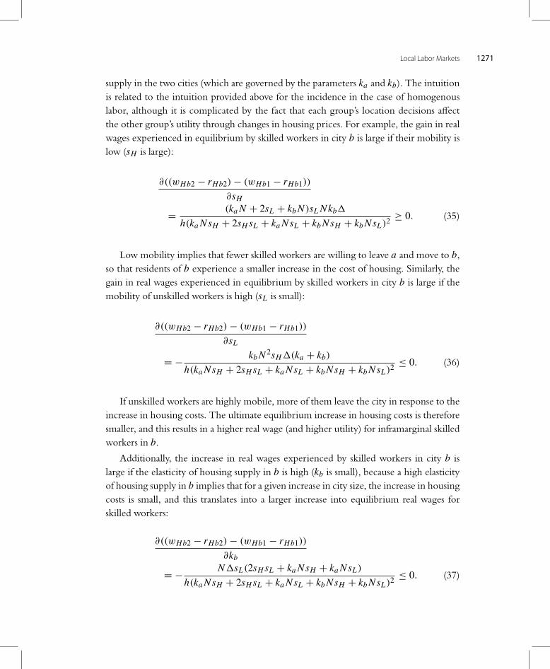
Local Labor Markets 1271
supply in the two cities (which are governed by the parameters ka and kb). The intuitionis related to the intuition provided above for the incidence in the case of homogenouslabor, although it is complicated by the fact that each group’s location decisions affectthe other group’s utility through changes in housing prices. For example, the gain in realwages experienced in equilibrium by skilled workers in city b is large if their mobility islow (sH is large):
∂((wHb2 − rHb2)− (wHb1 − rHb1))
∂sH
=(ka N + 2sL + kb N )sL Nkb1
h(ka NsH + 2sH sL + ka NsL + kb NsH + kb NsL)2≥ 0. (35)
Low mobility implies that fewer skilled workers are willing to leave a and move to b,
so that residents of b experience a smaller increase in the cost of housing. Similarly, thegain in real wages experienced in equilibrium by skilled workers in city b is large if themobility of unskilled workers is high (sL is small):
∂((wHb2 − rHb2)− (wHb1 − rHb1))
∂sL
= −kb N 2sH1(ka + kb)
h(ka NsH + 2sH sL + ka NsL + kb NsH + kb NsL)2≤ 0. (36)
If unskilled workers are highly mobile, more of them leave the city in response to theincrease in housing costs. The ultimate equilibrium increase in housing costs is thereforesmaller, and this results in a higher real wage (and higher utility) for inframarginal skilledworkers in b.
Additionally, the increase in real wages experienced by skilled workers in city b islarge if the elasticity of housing supply in b is high (kb is small), because a high elasticityof housing supply in b implies that for a given increase in city size, the increase in housingcosts is small, and this translates into a larger increase into equilibrium real wages forskilled workers:
∂((wHb2 − rHb2)− (wHb1 − rHb1))
∂kb
= −N1sL(2sH sL + ka NsH + ka NsL)
h(ka NsH + 2sH sL + ka NsL + kb NsH + kb NsL)2≤ 0. (37)
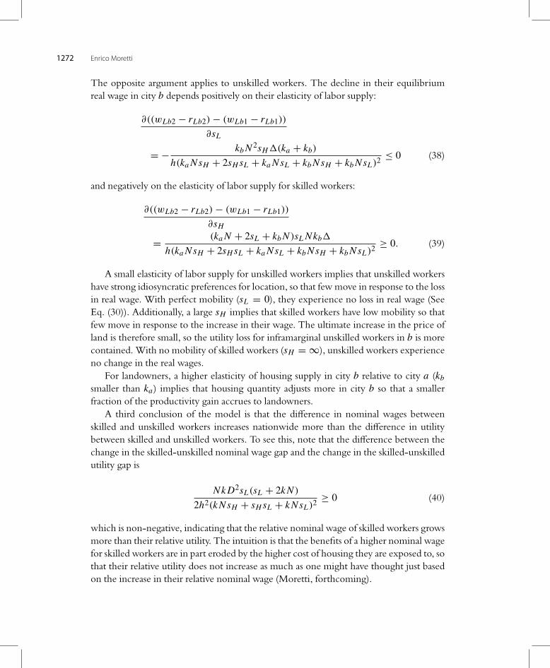
1272 Enrico Moretti
The opposite argument applies to unskilled workers. The decline in their equilibriumreal wage in city b depends positively on their elasticity of labor supply:
∂((wLb2 − rLb2)− (wLb1 − rLb1))
∂sL
= −kb N 2sH1(ka + kb)
h(ka NsH + 2sH sL + ka NsL + kb NsH + kb NsL)2≤ 0 (38)
and negatively on the elasticity of labor supply for skilled workers:
∂((wLb2 − rLb2)− (wLb1 − rLb1))
∂sH
=(ka N + 2sL + kb N )sL Nkb1
h(ka NsH + 2sH sL + ka NsL + kb NsH + kb NsL)2≥ 0. (39)
A small elasticity of labor supply for unskilled workers implies that unskilled workershave strong idiosyncratic preferences for location, so that few move in response to the lossin real wage. With perfect mobility (sL = 0), they experience no loss in real wage (SeeEq. (30)). Additionally, a large sH implies that skilled workers have low mobility so thatfew move in response to the increase in their wage. The ultimate increase in the price ofland is therefore small, so the utility loss for inframarginal unskilled workers in b is morecontained. With no mobility of skilled workers (sH = ∞), unskilled workers experienceno change in the real wages.
For landowners, a higher elasticity of housing supply in city b relative to city a (kb
smaller than ka) implies that housing quantity adjusts more in city b so that a smallerfraction of the productivity gain accrues to landowners.
A third conclusion of the model is that the difference in nominal wages betweenskilled and unskilled workers increases nationwide more than the difference in utilitybetween skilled and unskilled workers. To see this, note that the difference between thechange in the skilled-unskilled nominal wage gap and the change in the skilled-unskilledutility gap is
Nk D2sL(sL + 2k N )
2h2(k NsH + sH sL + k NsL)2≥ 0 (40)
which is non-negative, indicating that the relative nominal wage of skilled workers growsmore than their relative utility. The intuition is that the benefits of a higher nominal wagefor skilled workers are in part eroded by the higher cost of housing they are exposed to, sothat their relative utility does not increase as much as one might have thought just basedon the increase in their relative nominal wage (Moretti, forthcoming).
Local Labor Markets 1273
3.3. Spatial equilibriumwith agglomeration economiesIn Sections 3.1 and 3.2, the productivity of firms in the two cities is determined by thecity-specific productivity parameter Xc, which is taken as given. I now consider the casewhere there are agglomeration economies so that the productivity of firms in a locality isan endogenous function of the level of economic activity in that locality. This amountsto endogenizing the city-specific productivity shifter. For example, one can assume thatproductivity in a locality is a function of the number of workers in that locality, so thatXc = f (Nc) with f ′ > 0. In this case, the location decisions of workers generates apositive externality. In Section 4 I discuss in detail the possible sources of agglomerationeconomies.
As in Sections 3.1 and 3.2, a locality that is for some reason more productive attractsmore workers. But unlike Sections 3.1 and 3.2, the increase in population has theadditional effect of further increasing productivity of local firms. This in turn attracts evenmore workers and the process continues to the point where land prices are high enoughthat marginal workers and firms are made indifferent between locations. Most of theresults on incidence presented above remain true. The main difference with the previousanalysis is that the existence of agglomeration economies has the potential to generatemultiple equilibria, with some equilibria characterized by low economic activity, lowcost of housing and low nominal wages, and other equilibria characterized by higheconomic activity, high cost of housing and high nominal wages.32
For concreteness, consider the case of homogenous labor and assume a specificfunctional form for the agglomeration externality: Xc = xc+γ Nc, where the parameterγ governs the strength of agglomeration economies. In the version of the model withoutagglomeration spillovers (γ = 0), labor demand has the standard downward slopingshape (see Eq. (5)). With agglomeration spillovers, this is not necessarily the case.
Eq. (5) becomes
wc = xc + (γ − (1− h))Nc + (1− h)Kc + ln h. (41)
An increase in the number of workers employed in a city has two opposing effects.On the one hand, because of the standard assumptions on technology, an increase inthe number of workers lowers the marginal product of labor. On the other hand, theincrease in population raises labor productivity. If the agglomeration spillover is strongenough (γ > (1− h)), the labor demand function in a city may be upward sloping.
As in Section 3.1, assume that the two cities are identical in period 1, and that inperiod 2 city b experiences an exogenous increase in productivity of size 1, so that
32 Glaeser (2008) proposes a comprehensive theoretical equilibrium framework with agglomeration externalities. See alsoCombes et al. (2005) for a useful big-picture graphical treatment of spatial equilibrium with agglomeration economies.

1274 Enrico Moretti
xb2 = xb1 + 1. This initial increase in productivity pushes nominal wages up andhigher nominal wages attract more workers to city b. The arrival of new workers in city bgenerates productivity spillovers and, as a consequence, the initial productivity differenceis magnified.
It is informative to compare the equilibrium in the case where there are agglo-
meration spillovers (γ > 0) with the case where there are no spillovers (γ = 0). Inthe presence of spillovers, a productivity shock of size1 in city b results in an increase inthe equilibrium nominal wage that is larger than1:
wb2 − wb1 =h(N (ka + kb)+ 2s)− γ N
h(N (ka + kb)+ 2s)− 2γ N1 ≥ 1 ≥ 0. (42)
This is to be expected, because the agglomeration spillover magnifies the effect of theproductivity shock. By contrast, in the case with no spillovers (γ = 0), the increase innominal wage in city b is exactly equal to 1. (See Eq. (9)). Not surprisingly, the largeris the magnitude of the agglomeration spillover—i.e. the larger the parameter γ—thelarger is the ultimate increase in the equilibrium nominal wage in city b:
∂(wb2 − wb1)
∂γ=
Nh(N (ka + kb)+ 2s)1
(2γ N − 2hs − kb Nh − ka Nh)2≥ 0. (43)
Exactly as in Section 3.1, the higher productivity in city b attracts more workers there.
The number of workers in city b increases by
Nb2 − Nb1 =Nh
h(N (ka + kb)+ 2s)− 2γ N1 ≥ 0. (44)
Just as in the standard case without agglomeration spillovers, if housing supply is notinfinitely elastic, the increase in the population of city b ultimately results in higherhousing costs:
rb2 − rb1 =kb Nh
h(N (ka + kb)+ 2s)− 2γ N1 ≥ 0. (45)
It is obvious from Eqs (44) and (45) that the increase in city size and the consequentincrease in housing costs are larger the larger is the spillover (i.e. the large is γ ). If thespillover is zero, Eqs (44) and (45) revert to Eqs (8) and (10) in Section 3.1.
Since both nominal wages and housing costs increase in b, the ultimate effect on realwages is ambiguous and depends on whether the increase in nominal wage is larger orsmaller than the increase in housing costs. In particular, the change in the equilibrium

Local Labor Markets 1275
real wage is
(wb2 − wb1)− (rb2 − rb1) =(ka N + 2s)h − γ N
h(N (ka + kb)+ 2s)− 2γ N1 (46)
which is clearly smaller than the increase in nominal wage in Eq. (42). This equationindicates that the change in the real wage depends on the magnitude of the spilloverrelative to other parameters. To see exactly how the change in the equilibrium real wagedepends on γ , note that
∂((wb2 − wb1)− (rb2 − rb1))
∂γ=
Nh(N (ka − kb)+ 2s)1
(2γ N − 2hs − kb Nh − ka Nh)2(47)
which can be either positive or negative depending on whether (N (ka − kb)+ 2s) > 0or (N (ka − kb) + 2s) < 0. If the elasticity of housing supply in city b is larger or equalto the elasticity of housing supply in city a, the derivative is positive, indicating that thechange in the equilibrium real wage in city b is positively associated with the strengthof the agglomeration spillover γ . In this case, the increase in real wages in Eq. (46) forthe case of positive agglomeration spillovers is larger than the increase in real wages inEq. (11) for the case with no spillovers.
On the other hand, if the elasticity of housing supply in b is small enough relativeto the elasticity of housing supply a, the derivative is negative, and the change in theequilibrium real wage in city b is negatively associated with the strength of the spillover.33
Intuitively, if the elasticity of housing supply in b is small (large kb), housing prices in bincrease more following the productivity shock, and this increase lowers the equilibriumreal wages for a given increase in the nominal wage. In the extreme, if the elasticity ofhousing supply in b is zero (kb = ∞), the equilibrium real wage does not change. To seewhy, note that if the elasticity of housing supply in b is zero nobody can move to city bbecause no new housing unit can be added and Eqs (42) and (45) become
wb2 − wb1 = 1 (50)
33 The change in real wages in city a is smaller than the changein b:
(wa2 − wa1)− (ra2 − ra1) =ka Nh − γ N
h(N (ka + kb)+ 2s)− 2γ N1 ≥ 0. (48)
The derivative of this change with respect to γ is
∂((wa2 − wa1)− (ra2 − ra1))
∂γ=
Nh(N (ka − kb)− 2s)1
(2γ N − 2hs − kb Nh − ka Nh)2≥ 0. (49)

1276 Enrico Moretti
and
rb2 − rb1 = 1. (51)
In this case, the increase in the nominal wage is exactly equal to the productivity shock1 even in the presence of agglomeration spillovers because the constraint on labormobility effectively rules out endogenous changes in total factor productivity Xc. Theincrease in housing prices is exactly equal to the productivity shock 1 because the lackof any response in the supply of housing implies that the entire productivity shock getscapitalized into land prices. Since both nominal wages and housing cost increase by thesame amount1, Eq. (46) becomes
(wb2 − wb1)− (rb2 − rb1) = 0. (52)
In sum, even with agglomeration economies it is possible (although not necessary)to have a non degenerate equilibrium where both cities have positive population.Qualitatively, the incidence of the productivity shock is not very different from the casediscussed above where there are no agglomeration economies.
3.4. Spatial equilibriumwith tradable and non-tradable industriesIn the model presented above, the only consumption good is a homogenous tradablegood. In reality, however, cities produce and consume a variety of goods, both tradableand non-tradable. Here I discuss how this may affect the equilibrium. This discussion islargely based on Moretti (forthcoming).
Assume that there are K tradable industries producing goods x1, x2, x3, . . . , xK andM non-tradable industries, producing goods z1, z2, . . . , zM . Consider the case of apositive shock to productivity in tradable industry x1 in city c. The direct effect of thisshock is an increase in employment in industry x1. The indirect effect is a change inemployment both in the rest of the tradable sector and in the non-tradable sector.
Consider first the effect on the non-tradable sector. Following the shock to sectorx1, aggregate income in the city increases for two reasons. First, there are more localjobs; second, if local labor supply is upward sloping, as in Section 3.1, local wages arealso higher. The increase in the city budget constraint results in an increase in the localdemand for non-tradables z1, z2, . . . , zM . Employment in industries like restaurants,theaters, real estate, cleaning services, legal services, construction, medical services, retail,personal services, etc. grows both because the city has more workers and wages are higher.The magnitude of the multiplier effect depends on three factors. First, it depends onconsumer preferences for tradables and non-tradables and the technology in the non-
tradable sector. If preferences are such that a larger share of income is spent on locallyproduced non-tradables, the multiplier is larger, everything else constant. Similarly, amore labor intensive technology in the non-tradable sector results in a larger multiplier,

Local Labor Markets 1277
everything else constant. Second, it depends on the type of new jobs in the tradablesector. Adding skilled jobs in x1 should have a larger multiplier than adding unskilledjobs, because skilled jobs pay higher earnings and therefore generate a larger increase inthe demand for local services.
Third, there are offsetting general equilibrium effects on wages and prices. Asexplained in Sections 3.1 and 3.2, the magnitude of these effects ultimately depend onthe elasticities of local labor and housing supply. If those elasticities are not infinite, localwages, land prices and the price on non-tradables increase following the shock to x1.
In turn, this city-wide increase in labor and land costs causes a decline in the supply oflocal services. This decline partially—but not fully—undoes the effect of the increase indemand for local services. Effectively, the addition of jobs in x1 partially crowds out jobsin other industries. If labor supply is locally very elastic, this crowding out is more limitedand the increase in labor costs is small, making the multiplier larger.
The shock to industry x1 may also affect employment in tradable industriesx2, x3, . . . , xK , although the direction of the effect is unclear a priori. This effect isgoverned by three different forces. First, and most importantly, the city-wide increasein labor costs hurts employment in x2, x3, . . . , xK . Because these are tradable industries,the increase in production costs lowers their competitiveness. Unlike in the case of non-
tradable goods, the price of tradable goods is set on the national market and cannotadjust to local economic conditions. In the long run, some of the production in theseindustries is likely to be shifted to different cities. Second, the increase in production ofx1 may increase the local demand for intermediate goods and services. In this case, someelements of the vector x2, x3, . . . , xK are inputs to produce x1. This effect depends onthe geography of the industry supply chain. While many industries are geographicallyclustered, the magnitude of this effect is likely to be quantitatively limited if the marketfor x2, x3, . . . , xK is truly national. Third, if agglomeration economies are important, theincrease in production in sector x1 may result in more local agglomeration (see Section 4).
Carrington (1996), Moretti (forthcoming) and Black et al. (2005) estimate theemployment multiplier at the local level. Carrington (1996) focuses on the short-runmultiplier generated by the construction of the Trans-Alaskan Pipeline System. He findsevidence that the increase in construction jobs caused by the Trans-Alaskan PipelineSystem had significant multipliers for jobs in other parts of the non-tradable sector inAlaska. In contrast, Moretti (forthcoming) focuses on long-run multipliers. He quantifiesthe long-term change in the number of jobs in a city’s tradable and non-tradable sectorsgenerated by an exogenous increase in the number of jobs in the tradable sector, allowingfor the endogenous reallocation of factors and adjustment of prices. He finds that foreach additional job in manufacturing in a given city, 1.6 jobs are created in the non-
tradable sector in the same city. This effect is significantly larger for skilled jobs: addingone additional skilled job in the tradable sector generates 2.5 jobs in local goods andservices, while adding one additional unskilled job in the tradable sector generates 1 job
1278 Enrico Moretti
in local good and services. Industry-specific multipliers indicate that high-tech industrieshave the largest multiplier. Using a different time horizon, and focusing on time-varyinglocalized shocks to the coal mining sector, Black et al. (2005) uncover smaller multipliers.They find that each additional mining job generates 0.17 non-tradable jobs. Interestingly,the estimated effect is not symmetric. The loss of a mining job results in the loss of 0.34non-tradable jobs.
Theory suggests that the local multiplier for the tradable sector should be smallerthan the one for the non-tradable sector, and possibly even negative. Consistent with thishypothesis, Carrington (1996), Moretti (forthcoming) and Black et al. (2005) fail to findany significant effect of employment in the tradable sector.
The magnitude of local multipliers is important for regional economic developmentpolicies. It should be stressed, however, that the presence of large multipliers is not, initself, a market failure, and therefore does not necessarily justify government intervention.
3.5. Some empirical evidenceThe model presented in this Section appears to be general enough to capture many keyfeatures of a realistic spatial equilibrium. To get a better sense of how well the modeldescribes the real world, I now review some of the empirical evidence on the assumptionsand the predictions of the model.34
One type of labor The evidence in Bartik (1991), Blanchard and Katz (1992),and David et al. (1997) is broadly consistent with the predictions of the model withhomogenous labor in Section 3.1. These three papers aggregate all workers into onegroup and find substantial evidence of large labor flows following permanent labordemand shocks to a local labor market. Using state-level variation in demand conditions,Blanchard and Katz (1992) find that the main mechanism that re-establishes theequilibrium after a demand shock appears to be labor mobility, rather than job creationor job migration. Positive demand shocks are followed by substantial in-migration, whilenegative demand shocks are followed by substantial out-migration, up to the point thatthe original equilibrium between demand and supply is restored. In other words, theseshocks have permanent effects on the size of labor markets. Blanchard and Katz (1992)estimate that it takes slightly less than a decade for the affected state to return to the initialequilibrium after a localized shock. Bartik (1991) estimates suggest a somewhat sloweradjustment. The difference is in part due to the fact that the type of shocks examinedby Bartik and Blanchard and Katz is different. Both papers focus on permanent shocks.However, Bartik’s estimates come from a model where there is a “once-and-for-all shock
34 Glaeser and Gottlieb (2009) argue that the assumption and the conclusions of the spatial equilibrium model seemgenerally consistent with most first order facts about the US labor and housing markets. For example, geographicmobility in the US is significant, with more than 40% of households changing addresses every 5 years. Yet, Glaeser andGottlieb note that “there has been little tendency for people to move to high income areas” even in the presence oflarge wage disparities across areas. However, they caution that the fact that most amenities are hard to measure makesit inherently difficult to test conclusively whether the US labor market is indeed in a spatial equilibrium.

Local Labor Markets 1279
to local job growth, with subsequent growth unchanged from what it would have been”.By contrast, Blanchard and Katz’s estimates come from a model where the one-timeshock to local job growth is allowed to affect subsequent job growth.
Overall, the findings in Blanchard and Katz (1992) on wages and housing prices areconsistent with the version of the spatial equilibrium model where both local labor supplyand housing supply are quite elastic in the long run. In particular, following a negativeshock, nominal wages decline in the short run, but go back to their original level inthe long run. Housing prices track changes in nominal wages, so that the decline in realwages is limited.35
Topel (1986) generalizes the spatial equilibrium model to a dynamic setting.Consistent with Bartik (1991) and Blanchard and Katz (1992), Topel finds that positiveshocks to labor demand in a local labor market increase nominal wages there. But inaddition to the other two papers, Topel also finds that it is not just current shocksthat matter for current wages, but also expectations of future shocks. In particular, theexpectation of a future demand shock to a local labor market generates in-migrationto that market and therefore ultimately results in lower current nominal wages. Animplication is that wages respond more to transitory shocks to local labor markets than topermanent shocks.
More than one type of labor Topel (1986) is among the first to posit that mobilitycosts could be different across skill groups, with low-skilled workers having higher costsand suggest that this difference may affect the welfare incidence of demand shocks.Consistent with a version of the model with heterogenous labor in Section 3.2 wherethe propensity to move of unskilled workers is different from the propensity to moveof skilled workers, Topel finds evidence of a larger incidence of localized labor demandshocks on low-skilled workers than on high-skilled workers. In terms of the model thisimplies that sL > sH . Recall that the parameter s characterizes the amount of workerpreferences for location. A larger s implies a lower elasticity of local labor supply andtherefore lower labor mobility in response to economic shocks.36
Bound and Holzer (2000) find similar results. Using data on metropolitan areas,Bound and Holzer separately quantify the effects of location-specific labor demandshocks on the labor market outcomes of skilled and unskilled workers. As in Blanchardand Katz, Bound and Holzer (2000) find that positive (negative) labor demand shocksare followed by labor in-migration (out-migration). However, unskilled workers appearto be less sensitive to possible arbitrage opportunities and therefore less mobile followinggood and bad shocks. This difference in labor mobility has implications for the incidenceof the shock. Because of their stronger preferences for location, unskilled workers
35 Additionally, David et al. (1997) document that the speed of adjustment depends on the exact source of the demandshock.
36 Evidence in Machin et al. (2009) and in Malamud and Wozniak (2009) indicates that the difference in mobility ratesbetween educated and less educated workers may be causal.

1280 Enrico Moretti
experience significantly larger declines in nominal and real wages following negativedemand shocks than skilled workers.37 As a consequence, it appears that low skilledworkers end up suffering more from localized negative demand shocks than high-skilledworkers because they see their real wages fall while high-skilled workers move to betterlabor markets.
Notowidigdo (2010) proposes an alternative explanation for the difference inmobility and incidence between high and low-skilled workers. He posits that low-skilledworkers may be shielded from local labor demand shocks because of declining houseprices and public assistance programs. Public assistance programs are naturally tiltedtowards low-skilled workers. Housing price declines may also benefit low-skilled workersmore than high-skilled workers if low-skilled workers have higher expenditure shares onhousing. In this case, local labor demand shocks have smaller incidence on low-skilledworkers than high skilled workers.
Residents vs movers The spatial equilibrium model described above does a goodjob of characterizing the incidence of demand or supply shocks to a local labor market,when incidence is defined as the share of the gains or losses that accrues to workers andlandowners, or the share that accrues to each city. However, the model is poorly equippedto deal with the question of incidence when incidence is about which workers benefit orlose: migrants or original residents. For simplicity, my assumptions completely rule outany labor supply responses by residents, thus forcing all the employment adjustment tocome from mobility in and out of the city. Moreover, the model is a full-employmentmodel where involuntary unemployment is ruled out. In reality, however, it is possiblethat residents may change the amount of labor that they supply following local demandshocks.
The issue of who—between residents and migrants—ends up getting the newjobs created by a positive labor demand shock is clearly important in the presenceof involuntary unemployment. This issue is particularly important when thinkingabout policies aimed at increasing local employment, like local development policies.Implementing a local development policy that increases employment in an areaand benefits only migrants from outside the area is quite different politically fromimplementing a local development policy that benefits residents. This is particularly trueif the development policy is financed by local taxpayer money.
The literature disagrees on this point. On one hand, Renkow (2003, 2006) andPartridge et al. (2009) argue that the primary source of employment increases following
37 Bound and Holzer (2000) estimate that a 10% aggregate decline in labor demand in a city causes the nominal wageof high-school and college graduates to decline in the long run by 7% and 4%, respectively. The difference is evenlarger for younger workers. They also find declines in real wages for both groups, although smaller than the declines innominal wages. These findings are qualitatively consistent with the estimates in Blanchard and Katz (1992), but theyrequire an elasticity of local labor supply that is lower than the one implied by the estimates in Blanchard and Katz.
Similarly, Topel (1986) finds large wage changes following a localized shock for groups of workers with low mobility,and small wage changes for groups of workers with high mobility.

Local Labor Markets 1281
localized demand shocks comes from non-residents. The evidence in these studies,however, is not particularly convincing and is far from conclusive. A more convincingset of empirical studies is represented by Eberts and Stone (1992) and Bartik (1991,2001). These studies find significant increases in the labor force participation of residentsfollowing localized labor demand shocks. In a authoritative review of the literature,Bartik concludes that probably 25% of the new jobs are filled by increases in the laborforce participation of local residents in the long run, with the remaining 75% going tooutsiders. In other words, three out of four new jobs “in a region are filled by personswho otherwise would not have lived there”.
4. THE DETERMINANTS OF PRODUCTIVITY DIFFERENCES ACROSSLOCAL LABORMARKETS
In Section 2, I documented the large and persistent differences in labor market outcomesacross metropolitan areas in the US. In Section 3, I clarified how those differences canpersist in equilibrium in the long run, and who the ultimate beneficiaries of thosedifferences are. In that section, the focus is on the consequences of these differences,while the source of these differences is taken as given. City b is assumed to be moreproductive than city a for some exogenous reason and this higher productivity ultimatelyresults in more population, higher wages and higher housing costs.
In reality, however, most productivity differences within a country are unlikely to beexogenous. In this section, I discuss what might determine productivity differences acrosslocations within a country. Economists have long hypothesized that the concentrationof economic activity may be explained by agglomeration economies of some kind.Agglomeration of economic activity is particularly remarkable for industries that producetradable goods, because the areas where economic activity is concentrated are typicallycharacterized by high costs of labor and land. The observation that firms that producetradable goods locate in areas where economic activity is dense and labor and land costsare high is consistent with the notion that those areas enjoy agglomeration advantagesthat offset the higher production costs.
I review the existing empirical evidence on agglomeration economies, focusing ontwo related questions:
• What do we know about the magnitude of agglomeration economies? (Section 4.1)• What do we know about the micro mechanisms that generate agglomeration
economies? (Section 4.2)
The past two decades have seen significant amounts of effort devoted to answeringthese two questions. The key empirical challenge has been the possible existence ofunobserved features of localities that affect firm productivity even in the absence ofagglomeration economies. The main conclusion of this section is that the existingliterature has made some progress in empirically testing for the existence and quantifying
1282 Enrico Moretti
the magnitude of agglomeration economies, accounting for possible omitted variables.However, the channels that generate these economies remain more elusive. Muchremains to be done in terms of empirically understanding the exact mechanisms thatgenerate agglomerations of economic activity.
The discussion in this section focuses on papers that might be of particular interest tolabor economists. See Duranton and Puga (2004a,b), Rosenthal and Strange (2004) andGlaeser and Gottlieb (2009) for recent surveys that are more focused on urban economics.
4.1. Empirical estimates of agglomeration economiesTwo empirical approaches have been proposed to test for and quantify agglomerationeconomies. The first approach is based on the equilibrium location decisions of firmsand seeks to infer the importance of agglomeration forces from the observed geographicdistribution of employment. Empirically measuring the degree of agglomeration ofdifferent localities is not straightforward. Naive indexes of concentration are sensitiveto heterogeneity in firm size and in the size of the geographic areas for which data isavailable. In a landmark study, Ellison and Glaeser (1997) propose a “dartboard” stylemethodology for comparing the degree of geographic concentration across industries,accounting for differences in firm size and in the definition of geographic units. Theyfind that firms are spread quite unevenly across localities. Almost all industries appear tobe localized to some degree, although in many industries, the degree of localization isnot large. When industry is defined at the two digit level, high levels of concentration areobserved in the tobacco, textile and leather industries. Low levels of concentration areobserved in the paper, rubber and plastics, and fabricated metal products industries. In animportant follow up, Ellison et al. (forthcoming) use data from the Longitudinal ResearchDatabase to compute pairwise coagglomeration measurements for manufacturingindustries and relate these coagglomeration measurements to industry characteristics.They document that coagglomeration rates are higher between industries that areeconomically similar, suggesting that agglomeration advantages may depend both onphysical proximity and on economic linkages between firms. In a related study, Rosenthaland Strange (2003) measure the extent of agglomeration by focusing on the localizationdecisions of new plants. In the presence of mobility frictions, the localization of newplants is particularly informative because it is arguably less constrained by past localizationdecisions. The empirical results are consistent with the notion that agglomerationeconomies decline rapidly over space. Duranton and Overman (2005) propose analternative measure of agglomeration. Unlike the Ellison and Glaeser (1997) measure,the Duranton and Overman measure is based on a continuous measure of distance andtherefore does not depend on arbitrary definitions of geographic units. Using data fromthe UK, they confirm the existence of a significant amount of spatial agglomeration.38
38 In particular, they find that more than half of the 4-digit industries in the UK are characterized by a degree ofagglomeration that is statistically significant.

Local Labor Markets 1283
While these dartboard tests are informative in quantifying agglomeration, the mainchallenge in interpreting these tests is that firms base their location decisions on wheretheir profits are expected to be highest, and this could be due to spillovers, naturaladvantage, or other unobserved cost shifters. The mere existence of agglomeration isnot conclusive evidence of agglomeration economies. A second approach to testing foragglomeration economies directly asks whether productivity is higher in areas that areeconomically denser. An obvious difficulty is that productivity is an elusive quantity thatis hard to measure empirically. In practice, existing studies have used alternative measuresof productivity, including output per worker, wages and total factor productivity.
Using data on output per worker, Sveikauskas (1975) and Ciccone and Hall (1996)show that increases in employment density in a location are correlated with significantincreases in output per worker, although the lack of a solid identification strategyprecludes strong conclusions about causality. In an influential paper, Glaeser and Mare(2001) use wages to measure the marginal product of labor, and ask whether wagesare higher in large urban areas. Because they use a longitudinal dataset that followsworkers over an extended period of time, and some workers are observed moving inand out of urban areas, the authors are able to account for permanent unobserved workerheterogeneity. Consistent with the existence of agglomeration economies, Glaeser andMare’ find a significant wage premium associated with urban areas. The wage profilesof movers indicate that a significant fraction of the urban wage premium accrues toworkers over time and stays with them when they leave cities. This finding is consistentwith the notion that urban areas speed the accumulation of human capital and that asignificant part of the urban wage premium is due to faster productivity growth in urbanareas. On the other hand, using French data, Combes et al. (2009) find evidence ofsignificant sorting of high ability workers into urban areas. Estimates of the relationshipbetween wages and density conditional on worker fixed effects are 50% smaller than theunconditional relationship, indicating that at least half of the wage disparity across Frenchcities can be explained by worker quality.39
More recent work seeks to provide more direct evidence on the relationship betweenagglomeration and productivity by testing whether total factor productivity at the firmlevel is higher in denser areas. Studies in this group use longitudinal plant-level data toestimate firm-level production functions and test whether changes over time in plantoutput are systematically associated with changes in the characteristics of the area aroundthe plant, after controlling for changes in inputs. Henderson (2003) and Moretti (2004b)are early adopters of this approach. In particular, Henderson (2003) estimates plantlevel production functions for machinery and high-tech industries as a function of thedensity of other plants in the area, both in the same industry and in different industries.Identification is based on the longitudinal nature of the data. He finds that in the high-tech sector the number of establishments in an industry is positively associated with
39 See also Wheaton and Lewis (2002).

1284 Enrico Moretti
productivity, although this association is small for the machinery industry. As expected,
this association is stronger for plants belonging to single-establishment firms than forplants that belong to multi-establishment firms.
More recently, Greenstone et al. (forthcoming) provide direct estimates of the magni-tude of agglomeration economies by comparing the effect of attracting a new manu-
facturing establishment on the productivity of existing manufacturing establishments in acounty. They propose a novel identification strategy that relies not just on the longitudi-nal nature of the data but also on reported location rankings of profit-maximizing firmsto identify a valid counterfactual for what would have happened to the incumbent plants’productivity in the absence of the plant opening. Greenstone, Hornbeck and Morettifind that attracting a new manufacturing establishment to a county results in substantialincreases in productivity for existing establishments in that county. Figure 9 replicatestheir Fig. 1 and shows that five years after the new plant opened, incumbent plants expe-
rienced a 12% relative increase in TFP. Consistent with the spatial equilibrium model inSection 3, Greenstone et al. (forthcoming) find that the increased productivity enjoyedby existing plants comes at a cost, as quality-adjusted labor costs increase. As argued inSection 3, this increase is consistent with an upward sloping local supply of labor or anupward sloping supply of housing. Since manufacturing firms produce nationally tradedgoods and cannot raise output prices in response to higher input prices, the ultimateincrease in profits experienced by incumbents is smaller than the productivity increase.
A notable feature of the spatial distribution of economic activity is represented byindustry clustering, whereby firms tend to cluster near other “similar” firms (for example:
firms that sell similar products). The cluster of IT firms in Silicon Valley, biomedicalresearch in Boston, biotech in San Diego and San Francisco, financial firms in Wall Streetand London are notable examples. The findings in Greenstone, Hornbeck and Morettihave interesting implications for explaining the existence and persistence of industrialclusters. The estimated productivity spillover appears to increase with various measuresof economic proximity between the new plant and the incumbent plant. Because thedocumented increase in labor costs applies to all firms in the affected county, while themagnitude of the documented productivity spillovers is larger for pairs of plants that areeconomically closer, incumbent firms that are economically further away from otherfirms should become less profitable over time. In the long run, this process may resultin increased agglomeration of similar plants in each location.
Arzaghi and Henderson (2008) estimate the effect on the productivity of Manhattanadvertising agencies of locating near other advertising agencies. Consistent withthe model proposed by Lucas and Rossi Hansberg (2002), they find agglomerationeconomies characterized by extremely rapid spatial decay. Moreover, consistent with thespatial equilibrium model, the benefit of agglomeration appears to be at least partiallyoffset by higher land prices. In this industry, physical proximity appears to be beneficialbecause it facilitates networking. Interestingly, the magnitude of the productivity spillover

Local Labor Markets 1285
Winners vs. Losers
Difference: Winners – Losers
Year, relative to opening
Year, relative to opening
Winning coutries Losing coutries
–7 –6 –5 –4 –3 –2 –1 0 1 2 3 4 5
–7 –6 –5 –4 –3 –2 –1 0 1 2 3 4 5
0
0
–0.05
–0.05
–0.1
–0.15
0.05
0.1
0.05
0.1
Figure 9 Productivity of incumbent plants in counties with a new plant opening and counterfactualcounties, relative to the year of plant opening. Notes: This figure reproduces Figure 1 in Greenstoneet al. (forthcoming). The solid line in the toppanel shows average total factor productivity of incumbentplants in counties that successfully attract a new manufacturing plant. In Greenstone, Hornbeck andMoretti these are called winner counties. t = 0 represent the year of the new plant opening. Thedotted line in the top panel shows average total factor productivity of incumbent plants in countiesthat bid for the new plant, make it into the group of finalists but ultimately fail to attract the newplant. In Greenstone, Hornbeck and Moretti these are called loser counties. The bottom panel showsthe difference in average total factor productivity of incumbent plants between winner counties andloser counties.
appears to vary with firm quality, with higher quality agencies benefitting more fromnetworking than lower quality agencies.
Of course, not every productivity spillover is necessarily a market failure that requiresgovernment intervention. Spillovers that occur within a firm, for example, can be inprinciple internalized. Mas and Moretti (2009) explore how the productivity of a workervaries as a function of the productivity of her co-workers and find evidence of significantwithin-firm productivity spillovers. The introduction of a high productivity worker ina shift significantly raises the productivity of her co-workers. In particular, substitutinga worker with above average permanent productivity for a worker with below averagepermanent productivity is associated with a 1% increase in the effort of other workerson the same shift. While low productivity workers benefit from the presence of morecapable workers, the productivity of high-skilled workers is not hurt by the presence
1286 Enrico Moretti
of low-skilled co-workers. This type of spillover could be internalized by the firm byraising the salary of highly productive workers to reflect their external benefit on theproductivity of less productive workers.
While significant progress has been made in estimating agglomeration economiesusing plausible identifying assumptions, some authors have raised the concern thatthe observed higher productivity in dense areas may reflect selection due to increasedcompetition. For example, Melitz and Ottaviano (2008) develop a framework wherethe presence of a larger number of firms in larger markets increases competition and thisultimately causes less efficient firms to disappear. While this argument may apply to coun-tries, it seems less obvious that it should apply to cities within a country. Within a country,firms in the tradable sector compete with firms in other cities, so it seems unlikely thatlocal concentration offers a good measure of the relevant degree of competition. Indeed,Combes et al. (2009) provide recent convincing evidence in support this observation.40
4.2. Explanations of agglomeration economiesUnderstanding the ultimate causes of agglomeration economies is crucial tounderstanding persistent labor market differences across metropolitan areas. It is also veryimportant for policy, as I discuss in Section 5. Here, I review the theory and the evidenceon the three most relevant explanations that have been proposed for the agglomerationof economic activity: (1) advantages deriving from thick labor markets; (2) advantagesderiving from proximity to providers of intermediate non-tradable goods and services;(3) localized knowledge spillovers.41
4.2.1. Thick labormarketsThick markets have long been understood to be more attractive than thin markets whenfrictions of some type separate demand from supply. For example, in the influentialbarter model by Diamond (1982), the probability of finding a trading partner dependson the number of potential partners available, so that an increase in the thickness of themarket makes trade easier. This generates multiple steady state equilibria and, in each ofthem, the equilibrium level of production is not efficient. In the context of local labor
40 They use a generalization of the Melitz and Ottaviano (2008) model to distinguish between agglomeration economiesand firm selection. Using French data on manufacturing establishments, they find that firms in large cities are moreproductive than firms in small cities, but find no difference in the amount of selection between small and large cities.
41 Other explanations have been proposed for agglomeration economies, but they seem to be less relevant than the threedescribed above. Some concentration of economic activity may be explained by the presence of natural advantagesthat constrain specific productions to specific locations. In practice, while natural advantages may be important insome industries, they are unlikely to be important determinants of agglomeration in most industries. In an often citedpaper, Ellison and Glaeser (1999) show that natural advantages matter in some cases, but they account for only 20% ofthe observed degree of agglomeration. Historically, proximity of firms to consumers might also have played a role inthe agglomeration of economic activity in metropolitan areas (Krugman, 1991b). In practice, however, the substantialdecline in transportation costs makes this explanation less relevant for most industries at the present time. Glaeser andKohlhase (2003) calculate that the cost of moving goods by rail or trucking has declined more than 90 percent over thelast century.

Local Labor Markets 1287
markets, there are two reasons why workers and firms may find thick labor markets inlarge metropolitan areas attractive: better matches and lower risk.42
First, in the presence of worker and firm heterogeneity, a worker-firm match maybe more productive in areas where there are many firms offering jobs and many workerslooking for jobs. The higher quality of the worker-firm match in thicker labor marketsmay result in higher productivity and higher wages. This notion was first formalizedtwenty years ago in a model by Helsley and Strange (1990). Acemoglu (1997) andRotemberg and Saloner (2000) propose variants of this hypothesis. In Acemoglu’s model,employers in thick labor markets invest in new technologies because they know theycan find specialized employees. At the same time, employees in thick markets invest inhuman capital because they know that when they change jobs, their human capital willbe valued. Rotemberg and Saloner capture a similar idea in a model with multiple citieswith identical factor endowments. In their setting, agglomeration of production is causedby the fact that having more competition between firms to hire skilled workers makes iteasier for skilled workers to recoup the cost of acquiring industry-specific human capital.
Note that the relevant definition of labor market thickness is likely to depend not juston the size of a metropolitan area, but also on the skill set of a given worker. Two workerswith different skills living in the same metropolitan areas may be exposed to vastlydifferent labor market thickness. For example, a bioengineer and an architect living inthe same city may face different market thickness, depending on the local agglomerationof bioengineering firms and architectural firms.
A second potential benefit of thick labor markets is the provision of insuranceto workers and firms against idiosyncratic shocks. Thick labor markets reduce theprobability that a worker remains unemployed following an idiosyncratic negativeproduct demand shock to her employer. The presence of a large number of otheremployers implies a lower probability of not finding another job. At the same time,thick labor markets reduce the probability that a firm can’t fill a vacancy, following anidiosyncratic shock to the labor supply of an employee. The presence of a large numberof workers ensures a lower probability of not finding another worker. As in the case ofmatch quality, this argument applies particularly to workers with specialized skills.
These two versions of the thick labor market hypothesis have different empiricalimplications. If the size of the labor market leads to better worker-firm matches, weshould see that firms located in denser areas are more productive than otherwise identicalfirms located in less dense areas. The fact that the size of the labor market leads to a lowerrisk of unemployment for workers and a lower risk of unfilled vacancies for firms, doesnot imply differences in productivity between dense and less dense areas, but differencesin wages. The sign of these wage differences is unclear a priori, because it depends on themagnitude of the compensating differential that workers are willing to pay for lower risk
42 Labor market pooling externalities were first proposed by Marshall (1890).
1288 Enrico Moretti
of unemployment (generated by an increase in labor supply in denser areas) relative to thecost savings that firms experience due to lower risk of unfilled vacancies (generated by anincrease in labor demand in denser areas). The former can be thought of as an increasein labor demand in thicker markets, while the latter can be thought of as an increase inlabor supply in thicker markets.
Although the idea that thick labor market are beneficial is an old one, the existingempirical evidence is still limited. This is due in part to the fact that the quality of aworker-firm match has proven difficult to measure in practice.43 Using a semi-structuralmodel of the labor market, Petrongolo and Pissarides (2005) provide one of the earliesttests of the scale effect in job search based on the comparison of the number of jobmatches in labor markets of different sizes. The idea of the test is very simple. If thetotal number of vacancies and unemployed workers in a city is twice as large as the totalnumber of vacancies and unemployed workers in another city, we should see that thenumber of matches per unit of time in the former city is more than twice as large thenumber of matches in the latter. Using British data, Petrongolo and Pissarides comparethe offer arrival rate and the wage offer distribution in London (a thick labor market)with the rest of the country. They find significant scale effects in wage offers, but not inactual matches. However, the lack of observed scale effects in matches could in part beexplained if the reservation wage endogenously adjusts to the size of the market.
A second piece of empirical evidence has to do with the relationship betweenfrequency of job changes and size of the labor market. Wheeler (2008) and Bleakley andLin (2006) find evidence that, although indirect, is generally consistent with localizedincreasing returns to scale in matching. In particular, using longitudinal data from theNLSY, Wheeler (2008) documents that the probability of changing industry is positivelycorrelated with the size of the labor market for young workers and negatively associatedwith the size of the labor market for older workers. Bleakley and Lin (2006) find similarresults for industry and occupation changes using cross-sectional data from the Census.They also find that this pattern remains true even in the case of involuntary separations. Inother words, early in a career, when presumably workers are shopping around for a goodmatch, industry and occupation changes occur more often in large, diverse local marketsthan in small, specialized ones. Later in a career, when changing industry or occupationbecomes more costly because it may involve giving up specialized skills, industry andoccupation changes occur less often in large markets, presumably because matches arebetter. The existing evidence, while generally consistent with the notion that larger labormarkets facilitate matching, is still indirect. A more direct test might involve the durationof the match, as a measure of the quality of the match (Jovanovic and Rob, 1989). Atestable implication is that job duration should be longer in larger labor markets than insmaller markets.
43 In this respect, Puga (2009) argues that “the increasing availability of matched employer employee microdata willencourage more work on agglomeration through matching”.
Local Labor Markets 1289
An additional testable implication of this hypothesis is that the productivity benefitof thick labor markets should be particularly important for industries that rely onspecialized labor. Consider, for example, a digital media software engineer. If digitalmedia firms have heterogeneous technologies, and digital media software engineers haveheterogenous skills, it is likely that the match between a worker’s specific skills and a firm’sspecific technology is more productive in a city where there are many digital media firmsthan in a city where there is only one digital media firm.44 By contrast, the thickness ofthe labor market may not significantly improve the match quality and the productivityof less specialized workers in the same city, like manual laborers. An empirical test couldinvolve estimating the difference in the correlation between measures of match quality(for example, wages and job duration) and market size, for workers who live in the samecity but have different skill levels (specialized vs non specialized) and work in differentindustries (locally agglomerated vs locally non-agglomerated).
Fallick et al. (2006) posit that in high-tech industry clusters like Silicon Valley, highjob mobility may facilitate the reallocation of resources towards firms with superiorinnovations, but it may also create human capital externalities that reduce incentivesto invest in new knowledge. They argue that in the computer industry, the innovationbenefits of job-hopping exceed the costs from reduced incentives to invest in humancapital, while in other parts of the high-tech sector the opposite might be true. Theirevidence is consistent with this notion, but it is too indirect to be definitive.45
The evidence in Greenstone et al. (forthcoming) also is consistent with the notionthat spillovers occur between firms that share a similar worker pool. The magnitude ofthe productivity spillovers that they uncover depends on the economic linkages betweenthe new plant and the incumbent plant. In their data, spillovers are larger for pairs of firmsthat belong to industries that share the same set of workers. This lends credibility to thenotion that labor market pooling is an important source of agglomeration economies.
Costa and Kahn (2000) point out that thick labor markets are particularly importantfor dual career households, because thick labor markets may solve the co-locationproblem. The economic return of being in a large labor market relative to a smallmarket is increasing over time and Costa and Kahn attribute at least half of the increasedagglomeration of skilled workers in large cities to the growing severity of the co-locationproblem.
In his influential book on economic geography, Krugman (1991a,b) proposes analternative version of the thick labor market hypothesis. He argues that an advantage
44 Indirect support for this hypothesis can be found in Baumgardner (1988), who finds that doctors perform a narrowerand more specialized set of activities in large metropolitan areas than in small metropolitan areas.
45 Andersson et al. (2007) show that thicker urban labor markets are associated with more assortative matching betweenworkers and firms and argue that production complementarity and assortative matching are important sources of theurban productivity premium. Using a matched employer–employee database for Italy, Mion and Naticchioni (2009)also find important amount of assortative matching.
1290 Enrico Moretti
of thick labor markets is that idiosyncratic demand shocks to firms are less likely toaffect equilibrium wages. To see why it may matter, consider a firm experiencing anidiosyncratic positive productivity shock. If the labor market is thick, this firm faces arelatively flat supply of labor. If the labor market is thin, the firm faces an upward slopingsupply of labor and the firm-specific shock may ultimately result in higher labor costs.Consistent with this hypothesis, Overman and Puga (forthcoming) show that industriescharacterized by more idiosyncratic volatility are more spatially concentrated.
In sum, thickness of the labor market is a potentially promising explanation for theagglomeration of economic activity in metropolitan areas. It is highly plausible thatworkers prefer to be in areas with thick labor markets because of an increased probabilityof a better match with an employer and a reduction in the probability of unemployment.At the same time, it is also highly plausible that firms prefer to be in areas with thicklabor markets because of an increased probability of a better match with an employeeand a reduction in the probability of unfilled vacancies. While intriguing, most of theexisting empirical evidence is still quite indirect. This clearly is an area that should receiveincreased attention by labor economists in the years to come.
4.2.2. Thickmarket for intermediate inputsA second possible explanation for agglomeration economies centers on the availability ofspecialized intermediate inputs. Concentration of specialized industrial production cansupport the production of non-tradable specialized inputs. The agglomeration economyin this case is generated by the sharing of inputs whose production is characterized byinternal increasing returns to scale. This explanation is likely to be particularly relevant forfirms that utilize intermediate inputs that are both highly specialized and non-tradable.
Consider, for example, an industry where production crucially depends on the availabilityof specialized local producer services, such as specialized repair services, engineeringservices, venture capital financing, specialized legal support, or specialized shippingservices. To the extent that these services are non-tradable—or are costly to deliverto distant clients—new entrants in this industry have an incentive to locate near otherincumbents. By clustering near other similar firms, entrants can take advantage of anexisting network of intermediate inputs suppliers. In equilibrium, cheaper, faster or morespecialized supply of intermediate goods and services makes industrial clusters attractiveto firms, further increasing the agglomeration. This concentration process will go on upto the point where the increase in land costs offsets the benefits of agglomeration.
While this idea has been around for a long time, the first to formalize it are AbdelRahman and Fujita (1990), who propose a model where final goods are tradable, butintermediate inputs are non-tradable and are produced by a monopolistically competitiveindustry. In the model, firms that locate in dense areas share a larger and wider pool ofintermediate inputs suppliers, while otherwise similar firms that locate in rural areas sharea smaller and narrower pool of intermediate inputs suppliers. This difference generates

Local Labor Markets 1291
agglomeration advantages because an increase in the number of firms in an area results ina wider local supply of inputs and therefore in an increase in productivity.
The evidence in Holmes (1999) offers direct support for the input sharing hypothesis.Using data on manufacturing plants, he documents that manufacturing establishmentslocated in areas with many other establishments in the same industry make moreintensive use of purchased intermediate inputs than otherwise similar manufacturingestablishments in areas with fewer establishments in the same industry. Notably, thisrelationship only holds among industries that are geographically concentrated. Spatialproximity has limited impact on geographically dispersed industries.
Building on an idea first proposed by Rosenthal and Strange (2001), Overman andPuga (forthcoming) provide an alternative test of this hypothesis by relating measuresof geographic concentration for each industry to industry-specific measures of theimportance of input sharing. They find support for the notion that the availability oflocally supplied inputs is an important empirical determinant of industrial clusters.
Ellison et al. (forthcoming) propose an alternative approach to the one taken byRosenthal and Strange (2001) and Overman and Puga (forthcoming). They seek tounderstand the mechanics of the agglomeration process by focusing on how industriesare coagglomerated. Different agglomeration theories have different predictions aboutwhich pairs of industries should coagglomerate. For example, if input markets areimportant, then firms in an industry should be observed to locate near industries thatare their suppliers. On the other hand, if labor market pooling is important, thenindustries should locate near other industries that employ the same type of labor. Ellison,Glaeser and Kerr find evidence that input-output dependencies, labor pooling andknowledge spillovers are all significant determinants of agglomeration, but input-outputdependencies appear to be empirically the most important channel.
4.2.3. Knowledge spilloversEconomists have long speculated that the agglomeration of human capital may generatepositive spillovers, over and above its private effect.46 Different explanations have beenoffered for such spillovers. For example, physical proximity with educated workers maylead to better sharing of ideas, faster innovation or faster technology adoption. Perhapsthe most influential theoretical contribution in this area is the model by Lucas (1988).In that paper, human capital is assumed to have two effects. First, an individual’s ownhuman capital has the standard effect of increasing her own productivity. Second, theaverage aggregate level of human capital contributes to the productivity of all factors ofproduction. This second effect is an externality, because “though all benefit from it, noindividual human capital accumulation decision can have an appreciable effect on averagehuman capital, so no one will take it into account” in deciding how much to invest in
46 This question has important implications for education policies. The magnitude of the social return to education isimportant for assessing the efficiency of public investment in education.

1292 Enrico Moretti
human capital accumulation. In Lucas’ view, human capital externalities may be largeenough to explain long–run income differences between rich and poor countries. Whilein the model the externality is simply built into the production function in black-boxfashion, Lucas posits that the sharing of knowledge and skills through formal and informalinteraction may be the mechanism that generates the externality. More recent modelsbuild on this idea by assuming that individuals augment their human capital throughpairwise meetings with more skilled neighbors at which they exchange ideas. Examplesinclude Glaeser (1999),47 Jovanovic and Rob (1989), Henderson and Black (1999), Jaffeet al. (1993), Duranton and Puga (2001) and Saxenian (1994).48
A second class of models explains positive human capital externalities as pecuniaryexternalities that arise because of search or endogenous skill–biased technical change.Consider for example the case proposed by Acemoglu (1996), where job search is costly,and physical and human capital are complements. The privately optimal amount ofhuman capital depends on the amount of physical capital a worker expects to use. Theprivately optimal amount of physical capital depends on the supply of human capital. If agroup of workers in a city increases its level of education, firms in that city, expecting toemploy these workers, would invest more in physical capital. Since search is costly, someof the workers who have not increased their education would end up working with morephysical capital and hence earn more than similar workers in other cities. As in Lucas, thepresence of skilled workers in a city generates external benefits for other workers there.But what distinguishes Acemoglu’s story from Lucas’ story is that this result does notfollow from assumptions on the production function, but rather is derived from marketinteractions. Even though all the production functions of the economy exhibit constantreturns to scale in Acemoglu, the complementarity of human capital and physical capital,coupled with frictions in the job search process, generate a positive relationship betweenthe average wage and average human capital, holding constant workers’ individual humancapital.49
47 Glaeser (1999) argues that young workers move to cities because interactions with experienced workers help themincrease their human capital.
48 Of course, it is also possible that human capital externalities are negative. If education functions as a signal of productiveability, rather than enhancing productivity directly, the private return may exceed the social return. This is a casewhere people with higher innate ability signal their higher innate productivity by enduring extra years of schooling.
If schooling is more difficult for individuals with low innate productivity than for individuals with high innateproductivity, then, even if schooling itself is worthless in terms of enhancing productivity, it still may be a usefulscreening device for employers to identify more productive job applicants. In this case, increasing the average schoolingin a city would result in an increase in aggregate earnings that is smaller than the private return to schooling.
49 Although differences across cities in their quantity of physical capital play a central role in this model, differences in thequality of physical capital (technology) could arguably generate similar conclusions. Specifically, if skills and technologyare complementary, it is plausible to assume that the privately optimal amount of human capital depends not only on theamount of physical capital a worker expects to use, but also on the technological level that characterizes such capital.Similarly, in models with endogenous skill-biased technical change, an increase in the supply of educated workersincreases the size of the market for skill-complementary technologies and stimulates the R&D sector to spend moreeffort upgrading the productivity of skilled workers (Acemoglu, 1997).
Local Labor Markets 1293
There is growing empirical evidence that human capital spillovers and knowledgespillovers may be particularly important in certain high-tech industries, where innovationhas been shown to be linked to human capital externalities. Because human capitalspillovers and knowledge spillovers are invisible, most empirical studies resort to indirectevidence to test for the presence of spillovers. Jaffe et al. (1993) are an exception, inthat they provide direct evidence of spillovers using a “paper trail” based on patentcitations to test the extent to which knowledge spillovers are geographically localized.
Because patents are publicly available, in the absence of localized spillovers, citationsshould not depend on the location of the inventor. The key empirical challenge ofthe paper is to distinguish between geographic patterns of patent citations caused byspillovers from patterns caused by other sources of agglomeration effects. To address thisissue, the authors construct “control” samples of patents that have the same temporaland technological distribution as the patent citations and compare the two patterns ofgeographic concentration. They find that references to existing patents that inventorsinclude in their patent applications are likely to come from the same state or metropolitanarea as the originating patent application. They conclude that patent citations aregeographically localized and that knowledge spillovers appear to be large.
In a related study, Zucker et al. (1998) argue that the presence of specialized humancapital is the main determinant of the localization of biotechnology firms in the US.
They show that the stock of human capital of scientists in certain cities—measured interms of the number of publications reporting genetic-sequence discoveries in academicjournals—is correlated with the location of new biotech firms. This effect may reflect, atleast in part, human capital externalities, because it is not just a reflection of the presenceof universities and government research centers in areas where outstanding scientists arelocated. The introduction of new products—spatially clusters more in industries wherenew knowledge plays a more important role, holding constant the degree of spatialclustering of economic activity.50 In recent work, Carlino et al. (2007) use patents tomeasure innovation, and find that the number of patents per capita is positively correlatedto the density of employment in the highly urbanized portion of metropolitan areas. Acity with twice the employment density of another city has 20% more patents per capita.
Local human capital appears to be the most important predictor of per capita rates of
50 On the other hand, the exact magnitude of the spillovers is still debated. Audretsch and Feldman (1996) use data on theIPO’s of biotech firms to link the location of the biotechnology firm with the location of the university-based scientistsaffiliated with the firm. They conclude that “while proximity matters in establishing formal ties between university-
based scientists and companies, its influence is anything but overwhelming”. In earlier work, Adams and Jaffe (1996)study the composition of the knowledge transfers within and across firms. They use manufacturing plant-level data toexamine the productivity effects of R&D performed in a plant, outside a plant but inside the parent firm that ownsthe plant, and in external plants in the same geographic area or industry. They find that R&D of other firms in thesame industry is correlated with a plant’s own productivity, holding industry constant. However, identification is basedon questionable assumptions and the potential for omitted variable bias makes it hard to draw firm conclusions aboutcausality.

1294 Enrico Moretti
patenting. However, due to the absence of a credible research design, this study fails toestablish causality.
These earlier studies are consistent with the notion that knowledge spillovers maybe important in a limited number of high-tech or high-skill industries. More recentstudies seek to provide more general—and often better identified—tests for humancapital spillovers.
Using estimates of establishment-level production functions, Moretti (2004a) showsthat manufacturing plants are significantly more productive in cities with higher humancapital, holding constant individual plant human capital. The magnitude of spilloversbetween plants in the same city declines in economic distance as in Greenstone et al.(forthcoming). Much of the estimated spillover comes from high-tech plants. Fornon high-tech producers, the spillover appears to be limited. Consistent with thepredictions of the spatial equilibrium model, the productivity gains uncovered by Morettiappear to be offset by increased labor costs. The estimated productivity differencesbetween cities with high human capital and low human capital are similar to observeddifferences in wages of manufacturing workers, indicating an almost complete offset.While the documented productivity gains from human capital spillovers are statisticallyand economically meaningful, the implied contribution of human capital spillovers toeconomic growth does not appear to be large. Moretti estimates that human capitalspillovers were responsible for an average of a 0.1% increase in output per year duringthe 1980s.51
A recent paper by Beaudry et al. (2006) proposes a hypothesis that may potentiallyexplain Moretti’s findings. They argue that over the past 30 years, technological changeresulted in increases in the productivity of skilled workers in cities that had many educatedworkers. The estimates support the idea that differences in technology use across cities(measured by the adoption of computers) and its effects on wages reflect an equilibriumresponse to local factor supply conditions. In particular, cities initially endowed withrelatively abundant and cheap skilled labor adopted computers more aggressively thancities with relatively expensive skilled labor, causing returns to skill to increase most incities that adopted computers most intensively.
A growing number of studies focus on the effect of aggregate human capitalon earnings. A simple framework indicates that increases in the aggregate level ofhuman capital in a city have two distinct effects on wages. First, imperfect substitutionbetween educated and uneducated workers indicates that an increase in the number ofeducated workers will lower the wage of the educated and raise the wage of uneducatedworkers. Second, human capital spillovers may raise the wage of both groups. Imperfectsubstitution and spillovers both increase wages of uneducated workers, while the impactof an increase in the supply of educated workers on their own wage is determined
51 Glaeser et al. (1995) report that income per capita has grown faster in cities with high initial human capital in thepost-war period.

Local Labor Markets 1295
by two competing forces: the first is the conventional supply effect which makes theeconomy move along a downward sloping demand curve; the second is the spillover thatraises productivity. Using metropolitan areas as a definition of local labor markets, Rauch(1993) and Moretti (2004b), among others, document that wages are significantly higherin metropolitan areas with higher human capital, holding constant individual workerhuman capital. In particular, consistent with a model that includes both conventionaldemand and supply factors as well as human capital spillovers, Moretti finds that a onepercentage point increase in the labor force share of college graduates increases the wagesof high-school drop-outs, high-school graduates and college graduates by 1.9%, 1.6%and 0.4%, respectively. Using states as a definition of local labor markets, Acemoglu andAngrist (2000) fail to find significant evidence of human capital spillovers. A possibleexplanation of this difference is the evidence in recent work by Rosenthal and Strange(2008). They find that proximity to college graduates is associated with increases in wagesbut that these effects attenuate sharply with distance. If this is the case, it is possiblethat states are too large of geographic units to allow for the detection of human capitalspillovers.52
The findings in Glaeser and Mare (2001) described above are consistent with a modelwhere individuals acquire skills by interacting with one another, and dense urban areasincrease the probability of interaction. In a related paper, Peri (2002) shows that youngeducated workers receive a lower wage premium in urban areas than their old educatedworkers, but in spite of this, young educated workers are overrepresented in urban areas.Peri argues that learning externalities are an important explanation. Workers learn fromeach other when they are young, so living in dense urban areas may raise human capitalaccumulation more than living in a rural area. The negative compensating differentialindicates that young workers value such human capital externalities. As they grow older,the importance of knowledge spillovers diminishes, and some of them move toward non-urban areas.
Some studies have posited that areas with a more educated populace are more likelyto generate new business ideas and new firms. This is not a market failure. However,if skilled people are more likely to innovate in ways that employ other skilled people,this creates an agglomeration economy where skilled people want to be around eachother. Berry and Glaeser (2005) present evidence consistent with a model of urbanagglomeration where the number of entrepreneurs is a function of the number of skilledpeople working in an area. Consistent with this hypothesis, Doms et al. (2009) use anew panel of startup firms to show that areas that possess more skilled labor also possesshigher rates of self-employment and more skilled entrepreneurs. Moreover, conditional
52 Additionally, Acemoglu and Angrist estimate spillovers coming from high school graduation. On the contrary, Morettiand Rosenthal and Strange identify spillovers coming from variation in college graduation. It is possible that an increasein the number of those who finish high-school has a different external effect than an increase in the number of thosewho go to college.

1296 Enrico Moretti
on owner’s education, higher education levels in the local market are positively correlatedwith improved business outcomes.
5. IMPLICATIONS FOR POLICY
The empirical evidence surveyed in Section 4 points to the concrete possibility thatagglomeration of economic activity generates significant economies of scale at the locallevel. It is therefore natural to raise the question of the desirability of governmentintervention. In a world with vast disparities in income levels across localities and withsignificant agglomeration externalities, what is the proper role of economic policy?Should national or local governments provide subsidies to firms to locate in theirjurisdiction?
In this section, I discuss the economic rationales for location-based policies. I definelocation-based policies as government interventions aimed at reallocating resources fromone location to another location. These policies are widespread both in the US and inthe rest of the world. In the US, state and local governments spend $30-40 billion peryear on these policies, while the federal government spends $8-12 billion (Bartik, 2002).Examples of location-based policies typically adopted by local and state governmentsinclude direct subsidies and/or tax incentives for local firms, subsidized loans, industrialparks, technology transfer programs, export assistance and export financing, the provisionof infrastructure, workforce training, subsidies to higher education and area marketing.
Bartik (1991) provides a comprehensive taxonomy and discussion of the different typesof policies. More generally, states and cities compete based on income and corporatetax rates, labor and environmental regulations, and many other forms of interventionthat affect the relative profitability for firms of locating in each jurisdiction. The USfederal government also promotes several location-based policies. The Tennessee ValleyAuthority and the Appalachian Regional Commission are important historical examplesof large federal programs that target poor rural areas for development aid. A more recentexample is the Federal Empowerment Zones Program, which is a system of subsidiesfor businesses located in poor urban neighborhoods. Location-based policies are alsowidespread in Europe in the form of European Union regional transfers; and in Asia,
in the form of special economic zones.53
In general, economists think that there are two possible rationales for governmentintervention in the economy: equity and efficiency. Location-based policies areno exception. I begin in Section 5.1 by discussing several aspects of the equityrationale. In Section 5.2, I turn to the efficiency rationale. Bartik (1991, 2002) and
53 A prominent example of the latter is the successful program adopted by the government of Taiwan to subsidize R&Din semi-conductors and other high-tech fields.
Local Labor Markets 1297
Glaeser and Gottlieb (2009) provide authoritative discussions of the economic rationalesfor local subsidies with somewhat differing conclusions on their desirability.54
5.1. Equity considerations5.1.1. Incidence of subsidiesIt is tempting for policymakers to support policies intended to help disadvantaged areas.The main argument in favor of these policies is that by helping disadvantaged areas, thegovernment helps disadvantaged individuals. The spatial equilibrium model outlined inSection 3 suggests that this argument is at least in part flawed, since the poor are unlikelyto fully capture the benefits of location-based subsidies. In a world where workersare mobile, targeting locations instead of individuals is an ineffective way of helpingdisadvantaged individuals.
To see this more concretely, I consider first the case where subsidies for firms tolocate in a given locality are financed by the central government, and then the case wheresubsidies are financed locally.
(a) Centrally financed subsidies Consider a location-based redistributive policyintended to help disadvantaged areas. Assume for example that the central governmenttaxes residents of areas with high (nominal) income to provide subsidies to firmsto locate in areas with low (nominal) income. Most countries have these types ofredistributive policies. An example of this policy in the US is the Empowerment ZonesProgram mentioned above. Another example is represented by the ubiquitous statepolicies designed to attract businesses to poor parts of their jurisdiction. In Canada,an equalization program transfers income from high income provinces to low incomeprovinces. The European Union has a similar transfer program aimed at transferring EUdevelopment funds to regions with below average income.55
The incidence of this policy and its redistributive implications ultimately depend onthe elasticity of local labor supply and housing supply. Section 3 clarifies that if workersare highly mobile, they will arbitrage some or all of the benefits associated with thistransfer by relocating to the area favored by the transfer, thus bidding up the price ofhousing. In the case of high elasticity of local labor supply and less than infinite elasticityof housing supply, this increase in housing prices will offset most of the welfare gains thatmight otherwise accrue to existing residents.56 In the extreme case of perfect mobility,
54 Boarnet and Bogart (1996), Goolsbee and Maydew (2000), Faulk (2002), Bennmarker et al. (2009), Bondonio andEngberg (2000), Peters and Fisher (2002), Greenstone and Moretti (2004), Greenstone et al. (forthcoming) providerecent estimates of the employment effects of local subsidies. The last two papers have a discussion of the policyimplications of these subsidies. Work by Bartik (1991) and Papke (1993, 1994) represent important early contributionsthat helped to frame the policy debate on location-based policies in economic terms. See also Wasylenko (1997).
55 Similarly, one can think of a direct subsidy to residents of poor areas. For example, the national government could taxresidents of areas with high (nominal) income to provide a transfer to residents of areas with low (nominal) income.
This type of redistribution has similar implications.56 Of course, an infinitely elastic supply of housing would prevent this price increase.

1298 Enrico Moretti
increases in the price of housing fully offset the transfer. In this setting, location-basedredistributive policies intended to help areas with low nominal income have virtually noeffect on the utility of workers. The only beneficiaries of this policy are landowners inthe targeted areas. Effectively, this policy amounts to a transfer of wealth from landownersin the rest of the country to landowners in the targeted areas. If the theoretical model isa fair approximation of the real world, then its basic premises cast considerable doubt onthe desirability of redistributing income from areas with high income to areas with lowincome.57
How does this conclusion change if labor is not highly mobile? The model inSection 3 indicates that if individuals have significant preferences over specific locations,labor is less mobile. In this case, the marginal worker is indifferent across locations, butthe average worker is not and location-based redistributive policies have the potential toaffect the utility of the average worker. In particular, inframarginal workers in rich areasexperience an increase in taxes and a decrease in the cost of living, while inframarginalworkers in poor areas experience an increase in transfers and an increase in the cost ofliving. Overall, the redistributive effect is complicated and unlikely to be clear ex-ante,because it crucially depends on individual preferences for location, which are unlikely tobe observed by policy makers. This lack of observability makes it difficult to implementpolicies of this type in practice.
Busso et al. (2009) provide the first comprehensive empirical welfare analysis of alocation-based policy, namely the Empowerment Zones program. Using a remarkablydetailed series of data from the Census of Population, the Longitudinal Business databaseand the Standard Statistical Establishment List, together with an identification strategybased on areas that applied for the credits but did not receive it, they are able to crediblyquantify the incidence and deadweight loss of the program. Consistent with the spatialequilibrium model outlined in Section 3, they find that both wages and housing valuesincrease significantly in the neighborhoods that benefit from the federal subsidy relativeto the counterfactual neighborhoods in rejected zones. This increase is consistent withan upward sloping local supply of labor.
In terms of incidence, Busso et al. (2009) find that the program unambiguouslybenefits landowners in Empowerment Zone areas. This increase in housing values isnot particularly surprising. Together with the failure to find any changes in overall areapopulation, the increase in housing values indicates that the supply of housing is inelastic,at least in the short run. More surprisingly, the program also benefits workers who residein the area, since they experience an increase in nominal wages larger than the increasein housing costs. Based on the model in Section 3, this finding is consistent with the
57 In some cases, these types of policies may even have perverse consequences for targeted localities. Since the early 1970’s,the Canadian Unemployment Insurance program—a federal program—has been regionally differentiated, with moregenerous benefits in high unemployment areas. There is considerable evidence that this feature has had significantundesirable side effects. See Kuhn and Riddell (2010), for example.

Local Labor Markets 1299
presence of significant locational preferences on the part of residents. Workers who livein the targeted areas appear to have strong preferences for their current residence, so thattheir mobility is limited. This is notable, because the treated areas are neighborhoodswithin much larger metropolitan areas, and it is in principle possible to commute intothe Empowerment Zone areas from the rest of the metropolitan area without havingto change residence. Given the finding of small deadweight losses, the overall welfareassessment of the program appears encouraging.
Busso et al. (2009) also find that the provision of Empowerment Zone subsidies resultsin an increase in the productivity of local firms. While it is difficult to identify the exactchannel for this productivity increase, three plausible candidates are: an improvement inpublic infrastructure or other local public goods; some form of agglomeration economy;the role of the subsidies as a coordination mechanism for private investment. Because ofthe nature of the subsidy and the type of production that is common in empowermentzone areas, the most plausible candidate appears to be the last one.
(b) Locally financed subsidies I consider now the case where local taxpayers bearthe cost of subsidizing firms that locate in their jurisdiction. The welfare effects of thistype of policy depend on how similar the locations competing to attract new firms are. Inparticular, in the case of homogenous locations, a locally financed subsidy has no effect onresidents’ welfare since all the rent associated with the subsidy is transferred to the firm. Inthe case of heterogenous locations, a locally financed subsidy will benefit landowners byan amount proportional to the difference in production cost between the location withthe most desirable attributes and the location with the second most desirable attributes.The effect on workers depends on the importance of their preferences for location.Limited preferences for locations imply high mobility and therefore limited welfarechanges. Significant preferences for locations imply low mobility and therefore significantwelfare changes for inframarginal individuals.
To see this, I use the framework proposed by Greenstone and Moretti (2004). I assumethat local governments bid to attract new firms to their jurisdiction by offering subsidies,and that the cost of the subsidy is financed by increases in local property taxes, andtherefore is capitalized into land values. Let Vi j denote the benefit of the increase in thelevel of economic activity generated by new firm j for locality i , assumed to be known toall the other localities.58 Unlike in the case examined in the previous subsection—wherethe subsidy was paid for by the central government—here a successful bid now involves atrade-off for a locality. Let Ci j denote the direct monetary cost of the subsidy. The partialequilibrium change in welfare for the winning county can be expressed as Vi j − Ci j .
58 This is equal to the change in utility for local residents and landowners. If labor is mobile, workers are always indifferent,and landowners are the only set of agents whose welfare may be affected. If workers have preferences for location,
however, both workers and landowners are affected. While this type of subsidy is quite common in practice, itis not always obvious what localities seek to maximize in this process. One possibility is that, in the presence ofunemployment, localities seek to maximize job creation. My theoretical model in Section 3 is a full employmentmodel that by construction rules out unemployment.
1300 Enrico Moretti
Let the value to firm j of locating in county i be Zi j . Due to differences in technology,the same locality may be more or less attractive to different firms.59 A higher Zi j impliesthat the production costs of firm j are lower in locality i . I assume that Z is known toall localities. The total value for a firm of locating in a particular locality is the sum ofthe subsidy and the county-specific cost advantages. A firm will select the locality wherethis sum, Bi j + Zi j , is maximized. In order to obtain the highest subsidy, I assume thatthe firms conduct an English auction in the presence of independent, or private, values.I further assume that there is no collusion in the bidding among counties.
Consider the case where counties are homogeneous in V and Z : Vi j = V0 andZi j = Z0 for all i . In this case, the firm simply chooses the location that offers thehighest subsidy, B. The equilibrium bid, B∗, is B∗ = V0. This implies that successfullyattracting the firm does not change residents’ welfare: V0 − B∗ = 0. The reason is thateach jurisdiction keeps raising its bids until it is indifferent between winning and losing,so that the equilibrium bid is such that the entire economic rent is transferred to the firm.In this case landowners are indifferent, since the benefit of the new firm is fully offset bythe increase in property taxes. This result is similar to the result in the tax competitionliterature where local jurisdictions keep taxes on capital low because of a fear of capitalflight.
Consider now the more general case where counties’ valuations of attracting the plantand plants’ valuations of counties are heterogenous. Assume for simplicity that there areonly two locations, high V (VH ) and low V (VL ); and two levels of Z , high Z (Z H ) andlow Z , (ZL ). If V and Z are positively correlated, the location with high V also has highZ . In this case, this location gains the most from attracting firm j and it is also the mostattractive to firm j . The optimal bid is such that the firm is indifferent between movingto either city. Unlike the homogenous case, where all the economic rent is bid away,in this case, the H county enjoys an economic rent that comes from the fact that it hascharacteristics that are desirable to the firm.
If labor is highly mobile, and housing is inelastically supplied, this economic rentwill be capitalized into land values. In particular, land values increase by an amount(VH − VL) + (Z H − ZL) > 0, proportional to the difference in V and the differencein Z . The same intuition applies to the case where V and Z are negatively correlated,and location 1 has high V and low Z , while location 2 has high Z and low V . IfVH + ZL > VL + Z H , location 1 wins the firm by bidding an amount B∗ that makes thefirm indifferent: B∗ = VL+(Z H− ZL). As in the case of positive correlation between Zand V, the winning location enjoys a rent that is capitalized in land values, although therent is lower than the rent in the case of positive correlation: (VH−VL)−(Z H−ZL) > 0.A similar conclusion applies if VH + ZL < VL+ Z H . In this case location 2 is the winnerand its land prices increase by (Z H − ZL)− (VH − VL) > 0.
59 For example, the presence of a harbor, an airport or a freeway may be more important for some productions thanothers. Similarly, the presence of stringent environmental or labor regulations may affect some firms more than others.

Local Labor Markets 1301
5.1.2. Taxes and transfers based on nominal incomeAn important redistributive implication of the spatial equilibrium model has to do withfederal taxation and federal transfers. Federal taxes and transfers are calculated based onnominal income. By setting taxes and federal transfers in nominal terms, the federalgovernment engages in a hidden form of location-based redistribution, because workerswith the same real income pay higher federal taxes in high-cost areas than in low-costareas. Albouy (2009) estimates that workers in cities where nominal wages are above thenational average pay up to 27% more in federal taxes than similar workers in cities wherenominal wages are below the national average. As a consequence, $270 billion each yearare transferred from areas with high nominal wages to areas with low nominal wages.
In equilibrium, if workers are mobile, wages and land prices should adjust tocompensate workers. However, the resulting geographic distribution of employment isinefficient, since it penalizes highly productive cities and favors less productive cities.In other words, this policy artificially lowers economic activity and property values incities where labor is more productive and nominal wages are higher. At the same time itincreases economic activity and property values in cities where labor is less productive andnominal wages are lower. The net result is a loss in overall welfare. Albouy calculates thatthe long-run employment loss in high nominal wage areas is about 13%, while the lossin land and housing values is about 21% and 5%, respectively. Albouy suggests that onesolution is to make taxes independent of where workers live so that they are effectivelylump sum location-wise.
A related problem arises when thinking about transfer payments. Should they bebased on nominal or real income? Using a spatial equilibrium model similar to the one inSection 3, Glaeser (1998) derives the conditions under which welfare payments should beadjusted for differences in the local cost of living. He concludes that the optimal transferdepends on mobility and preferences for amenities. In the case of perfect mobility, transferpayments that correct for differences in the local cost of living are inefficient, because theyend up being capitalized in the price of land, further raising land costs in expensive areas.With limited mobility, a correction for local cost of living differences is optimal underthe assumption that amenities and income are complements.
5.1.3. Nominal and real differences across skill groups and regionsThe spatial equilibrium model has implications for how one should measure earnings andincome differences between skill groups or between regions. In most countries, there arelarge cost of living differences across regions. These differences are typically largely drivenby differences in the price of land. When comparing earnings or income across skillgroups or across regions, the question arises of whether nominal measures should be usedor whether real measures should be used. This question matters because the magnitudeof income differences between skill groups or between regions has implications for thedesirability of redistributive policies.
1302 Enrico Moretti
Earnings differences between skill groups Consider the increase in earningsinequality in the US labor market in the past three decades. As documented by a largeliterature in labor economics, starting in 1980 the nominal earnings of skilled workershave grown significantly faster than the nominal earnings of unskilled workers. In thesame period, there have been increasing differences in the geographic distribution ofskilled and unskilled workers. Skilled workers have increasingly concentrated in citieswith high costs of land, while unskilled workers have increasingly concentrated in citieswith low costs of land. This geographic sorting suggests that skilled workers might haveexperienced higher increases in the cost of living.
Consistent with this hypothesis, Moretti (forthcoming) finds that earnings inequalitymeasured in real terms has grown significantly less than earnings inequality in nominalterms. The model in Section 3 shows that the implications for utility inequality dependon the underlying reasons for the geographic sorting. If the sorting of skilled workersinto more expensive cities is driven by increases in the relative demand of skilled labor inthose cities, the increase in relative utility of skilled workers is smaller than the increasein their nominal wage. On the other hand, if the sorting of college graduates into moreexpensive cities is driven by an increase in the relative supply for skilled labor in thosecities (i.e. an increase in the attraction of local amenities), increases in the cost of living inthese cities reflect the increased attractiveness of the cities for skilled workers. In this case,there may still be a significant increase in utility inequality even if the increase in real wageinequality is limited. Moretti (forthcoming) argues that the evidence is more consistentwith the notion that shifts in the relative demand for skilled labor are the main forcedriving changes in the number of skilled workers across metropolitan areas and that theincrease in well-being inequality is smaller than the increase in nominal wage inequality.These results are related to a paper by Black et al. (2005) which, along with earlier workby Dahl (2002), criticizes the standard practice of treating the returns to education asuniform across locations. They show that, in theory, the return to schooling is constantacross locations only in the special case of homothetic preferences, and argue that thereturns to education are empirically lower in high-amenity locations.60
Regional differences in income and poverty A related question arises whenmeasuring earnings or income differences across locations. Using data for five US regions,Slesnick (2002) shows that regional comparisons of poverty rates based on nominalfigures give a different picture than regional comparisons of poverty rates based on realfigures. Consistent with the spatial equilibrium model, Slesnick shows that disparities inreal income across regions are smaller when cost of living differentials are accounted for,so that the prevalence of poverty across regions changes significantly. For example, rural
60 In a related paper, Black et al. (2009) argue that estimates of the wage differences between blacks and whites need toaccount for differences in the geographic location of different racial groups. They argue that accounting for geographychanges the estimates of the speed of convergence between black and white earnings. They also develop a theoreticalmodel to understand when estimates of the black-white earnings gap can be used to infer welfare differences.
Local Labor Markets 1303
areas and Southern states have a relatively low cost of living. As a consequence, povertyrates for rural areas and for many urban areas in the South are significantly closer to therest of the country when real income is used instead of nominal income.
While this evidence is a useful first step, it is likely that an analysis at the regional levelmisses important intra-regional variation in the cost of living. A geographically moredetailed analysis based on city-level data may uncover an even stronger effect of cost ofliving differences on the geographic distribution of poverty rates.
5.1.4. Subsidies to human capital when labor is mobileIn the spatial equilibrium model, workers’ mobility determines the incidence of location-
based government policies through their effects on land prices. Areas that benefit fromgovernment transfers experience an increase in the price of land that offsets (at leastin part) the benefit of the transfer. However, in reality, workers’ mobility may affectthe incidence of location-based government policies even in the absence of local pricechanges. A salient example is the case of subsidies to human capital accumulation.
Localized human capital externalities of the type discussed in Section 4.2.3 representan important efficiency rationale for the provision of public subsidies to investment inhuman capital. However, in the presence of significant worker mobility it is not clear whoultimately benefits from these subsidies. Consider for example the case of subsidies tohigher education. State and local government cover a larger fraction of higher educationexpenditures.61 Yet, the high mobility of educated workers across states implies that partof the investment in human capital made by one state may benefit other states. Boundet al. (2004) quantify the magnitude of this problem by relating the production of newcollege graduates in a state to the stock of college-educated workers in the state. Theyfind that the elasticity of stocks to flows is approximately 0.3 for BA’s. This elasticity iseven lower for students with medical degrees. This implies a high degree of migration.
In a simple static model of where the supply and demand for college graduates determinethe stock of college graduates, increases in the stock of college graduates due to increasesin supply should lead to lower relative wages for college graduates, whereas increases inthe stock due to increased demand should result in higher wages. The empirical results inBound et al. (2004) are consistent with the prediction that inelastic local demand causesthe effect of flows on stocks to be smaller. Additionally, a regression of relative wageson relative stocks indicates that the elasticity of wages to stocks is negative, consistentwith some areas exporting college graduates and others importing them. Using morerecent data, Bartik (2009) finds lower mobility rates of skilled workers and thereforeconcludes that state investment in higher education is not completely dissipated bylabor mobility.
61 For example, the current subsidy of direct costs to students at major public universities in the US is around 80%.

1304 Enrico Moretti
5.2. Efficiency considerationsThe previous subsection concluded that the equity rationale for public transfers thattarget locations instead of individuals is generally not very compelling. A second possiblerationale for government intervention has to do with efficiency. The key question in thisrespect is: are there market failures that suggest that governments should use taxpayermoney to provide efficiency enhancing subsidies to firms to locate in their jurisdiction?In the absence of significant market failures, it is difficult to justify the use of taxpayermoney for subsidies based on efficiency grounds. Here I consider four possible marketfailures.
5.2.1. Internalizing agglomeration spilloversLocal economic development policies are carried out both by local governments andby national governments.62 To draw normative implications, it is therefore importantto distinguish the point of view of a locality—which maximizes its own local welfarewithout consideration for aggregate welfare—from the point of view of the centralgovernment, which maximizes aggregate welfare.
Local welfare From the point of view of a local government, the mostimportant efficiency rationale for location-based incentives is the existence of significantagglomeration externalities. This rationale hinges on whether the attraction of newbusinesses generates some form of external benefits to other firms in the same locality.If the attraction of new business generates localized positive agglomeration externalities,then the provision of subsidies may be able to generate the efficient allocation of resourcesin the local economy.63
In a static setting, the optimal magnitude of these incentives depends on themagnitude of agglomerations externalities. The literature described in Sections 4.1 and4.2 suggests that these externalities may be important empirically, although there is stilldebate on their exact magnitude and the mechanisms that generate them.
In a dynamic setting, the existence of significant agglomeration economies has thepotential to generate multiple equilibria. Kline (2010) proposes a simple theoreticalframework that is useful in thinking about the magnitude of the efficient subsidy inthe presence of multiple equilibria. In this case, the magnitude of the optimal subsidyis more complicated to derive, because it depends on the exact shape of Marshallian
62 In the case of the European Union, some location-based policies are financed by the Union itself, which is aninternational government.
63 An additional, although arguably less important, rationale that has been proposed for subsidies to attract new firms—and especially headquarters—has to do with charitable contributions. Card et al. (2007) document that attracting theheadquarters of a publicly traded firm yields $3-10 million per year in contributions to local non-profits. Most of theincrease in charitable contributions appears to be linked to the number of highly-compensated individuals in a city,rather than through direct donations by the corporations themselves. From a normative point of view, this rationale isnot unassailable. Given the magnitude of the subsidies often required to attract headquarters, if this was the only benefitof attracting headquarters, there is no reason why the municipality should not have provided subsidies directly to thenon-profit sector.
Local Labor Markets 1305
dynamics. Consider for example the case where the productivity of firms in a localityis a function of the number of other similar firms in that locality so that attracting newfirms to a locality raises the productivity of all the firms in that locality (as in Greenstoneet al., forthcoming). If the magnitude of this agglomeration externality is large enough,it is possible that the demand for labor is locally upward sloping, since more firms ina locality imply both more workers and higher productivity (as in Eq. (41) above). Asdiscussed in Section 3.3, this setting is inherently characterized by multiple equilibria,with some equilibria featuring low levels of economic activity, low productivity andlow nominal wages and other equilibria featuring high levels of economic activity,high productivity and high nominal wages. The size of the efficient subsidy can varyenormously, depending on the exact functional form of Marshallian dynamics, and onthe starting point. On the one hand, if a locality is located at an unstable tipping point, avery limited subsidy can be enough to move it to a new equilibrium with an higher levelof economic activity and agglomeration. On the other hand, if a locality is trapped in astable bad equilibrium, “Big Push” type of policies may be needed to move it to a goodequilibrium (Kline, 2010).
In this context, government intervention in the form of subsidies for firms to locatein the jurisdiction has the potential to start an agglomeration process that can ultimatelyshift a locality from a bad equilibrium (small agglomeration, low productivity) to a goodequilibrium (large agglomeration, high productivity). The provision of a subsidy can havesubstantial and long lasting effects on the equilibrium level of economic activity in alocality.64 Indeed, the expectation of government intervention alone may play a role inshifting a locality from a bad to a good equilibrium. In this case, the government policyacts as a coordination mechanism that signals to workers and firms which locality amongall existing localities will move to a good equilibrium in the future. If firms and workerstake this signal as credible, they will move to that jurisdiction, effectively realizing theexpected outcome. In practice, it is implausible to expect that announcements alone areeffective enough to have substantial real-world effects on the localization of economicactivity. But it is plausible to think that in the presence of multiple equilibria, expectationstogether with the actual provision of subsidies might play a non-trivial role in thelocalization of firms and workers across locations.
In the presence of multiple equilibria, the efficiency benefits for location-basedpolicies have the potential to be quite large relative to the efficiency costs. Consider thecase where the provision of location based subsidies attracts new businesses to a locationand move the locality from a bad equilibrium (low density of economic activity) to a goodequilibrium (high density of economic activity). In this case the short-run efficiency costsof providing location-based subsidies could be small compared to the potential long-runbenefits of moving to a better equilibrium.
64 Of course, the process of agglomeration in this case would continue up to the point where the productivity advantagesof agglomeration are offset by the increase in land prices (Section 3.3).
1306 Enrico Moretti
Aggregate welfare The efficiency argument, however, has different implications ifone takes the point of view of the national government instead of the local government.For the point of view of a national government, the main concern is that the provision ofsubsidies by local governments may result in a zero-sum game, where the jobs created intargeted areas come at the expense of jobs elsewhere. In this context, justifying suchpolicies requires a rationale for moving jobs from one location to another. In theircomprehensive overview of the issue, Glaeser and Gottlieb (2009) argue that the onlysuch rationale is for local agglomeration economies to be stronger on the margin intargeted areas. In other words, aggregate efficiency would require subsidies to favorareas that are more productive and where the elasticity of productivity with respect toagglomeration is higher. To achieve this efficient allocation, policy makers need to knowthe exact functional form of the spillover function. In practice, this functional form isstill largely unknown, because it is difficult to estimate credibly. Given the difficulty ofidentifying the magnitude of agglomeration economies under a linearity assumption, itis not surprising that we still do not have a good idea of possible nonlinearities. Because ofthis difficulty, Glaeser and Gottleib conclude that policy-makers still do not have enoughinformation to implement location-based policies that are efficient from the aggregatepoint of view.
However, when the benefits of attracting a new firm are highly heterogeneous,it is in principle possible that competition among localities may result in aggregateefficiency gains. Greenstone et al. (forthcoming) document one example of significantheterogeneity in productivity spillovers. Using the methodology described inSection 4.1, they present location-specific estimates of the impact on TFP of incumbentplants of new plant openings. Their Fig 2. reveals that there is substantial heterogeneityin the estimated spillover. Importantly, the magnitude of the productivity spillover doesnot appear to be random, but it varies systematically with easily observable features ofthe new plant. In particular, Greenstone, Hornbeck and Moretti document that theproductivity spillover generated by the opening of a new large manufacturing plant islarger for incumbent plants that share similar labor and technology pools with the newplant.65 It appears plausible in this case that policy makers are able to evaluate the potentialvalue to their locality of attracting the new plant because this value depends on the degreeof proximity of the local labor and technology pools to those of the new plant. This typeof heterogeneity is important because it allows for the possibility of aggregate efficiencygains. National welfare is maximized when payments are made to plants that producethe spillovers so that they internalize this externality in making their location decision.In this case the locality that has the most to gain is the one that successfully attracts thenew plant. The decentralized equilibrium in the presence of significant heterogeneity in
65 By contrast, using a different methodology Glaeser and Gottlieb (2009) find little evidence that agglomerationeconomies vary systematically based on the easily observable characteristics of metropolitan areas. For example, theyfind that agglomeration economies do not appear to depend on city size or on urban amenities.

Local Labor Markets 1307
productivity spillovers together with the assumption that the potential value of attractingthe new plant is known to each locality is not necessarily inconsistent with aggregateefficiency. From the equity point of view, the discussion of a locally financed subsidy inSection 5.1.1 suggests that in this case some but not all of the economic rent generatedby the spillover ends up being transferred to the new firm. In particular, the locality thathas the most to gain should only capture the fraction of the overall benefit that reflectsthe difference in production costs between the location with the most desirable attributesand the location with the second most desirable attributes.
5.2.2. Unemployment, missing insurance and credit constraintsBesides the existence of agglomeration externalities, there are three additional marketfailures that can in principle justify location-based policies.
First, wages may not be fully responsive to local shocks. Consider the case ofidiosyncratic shocks to localities, where some cities or states are hit by negative demandshocks while other are not. The theoretical model in Section 3 is a full employmentmodel, where wages always adjust fully to local shocks. The model indicates that ifworkers are mobile, and wages fully adjust, counter-cyclical transfers to localities hit bynegative shocks will only have a limited effect on workers’ welfare. However, the modeleffectively assumes away unemployment. In reality, wages may not be fully responsive tolocal labor market conditions, at least in the short run. If wages are not fully responsive,negative demand shocks will cause socially costly involuntary unemployment. In thiscase, countercyclical transfers from the central government have the potential to improveaggregate welfare. Of course, this potential welfare gain should be weighed against thedistortionary cost of government intervention.
Second, even with full employment, homeowners are exposed to localized demandshocks, and there is no market-provided insurance to insure against such shocks. Asexplained in Section 3, shocks to a local economy affect the residents’ value of housing,unless the elasticity of housing supply is infinite. Since housing is the most importantasset for most households, the amount of risk generated by these shocks can be large.Existing financial instruments make it difficult to diversify housing risk. In this context,redistributive countercyclical policies that are centrally financed and target localities hitby negative idiosyncratic shocks may in principle act as government-provided insuranceagainst housing value risk that the market does not insure. This policy effectively acts asa redistributive mechanism that transfers resources from homeowners in areas affected bypositive shocks to homeowners in areas affected by negative shocks, thus reducing risk.
However, it is not clear that in practice these policies improve efficiency. First, there isthe general deadweight loss of government intervention. Second, and more importantly,homeowners and workers often coincide. An optimal insurance scheme should thereforetake into account both housing risk and wage risk. This is very difficult to do inpractice because the correlation between housing values and wages is complicated. Forexample, the model with heterogenous labor in Section 3 has shown that if workers

1308 Enrico Moretti
have idiosyncratic preferences for location, the effect of a localized shock on a worker’swelfare depends on that worker’s skill level and location. If labor and housing supplyelasticities are less then infinite, inframarginal skilled workers in the locality that receivesa positive skill-biased productivity shock (city b) experience an increase in utility, whileinframarginal unskilled workers experience a decrease. Inframarginal workers in city a,
the city not directly affected by the shock, experience an increase in utility, irrespective oftheir skill level. In other words, in the example of the model, wages and housing values arenegatively correlated for unskilled workers and for skilled workers in city a, but positivelycorrelated for skilled workers in city b. This makes an efficient location-based insurancepolicy difficult to implement in practice.
Finally, the private and social costs of mobility might not be the same. When workersare mobile, and the private cost of mobility and the social cost of mobility are identical,the spatial adjustment that follows a negative shock to an area may be efficient. However,as pointed out by Blanchard and Katz (1992), credit constraints may introduce a wedgebetween the private and social costs of mobility. For example, following a negative shockto an area, workers without access to credit may be forced to leave even when it is optimalfor them to borrow and wait for the equilibrium to be reestablished. This would lead toa socially inefficient degree of adjustment through mobility and may provide justificationfor efficiency-enhancing government intervention.
6. CONCLUSIONS
Understanding local labor markets is important for labor economists. The last threedecades have witnessed a growing amount of empirical research on the causes andconsequences of localization of workers and firms within a country. This area, at theintersection of labor and urban economics, contains important but challenging questionsand is likely to generate an increasing share of high quality empirical research in the nextdecade.
Besides the obvious relevance for labor economists directly working on these topics,the idea of spatial equilibrium discussed in this chapter has a broader relevance for laboreconomists in general. It is difficult to understand the effect of nationwide labor demandchanges on wages and employment without considering the role played by the spatialreallocation of labor and general equilibrium effects on local prices. Labor flows acrosslocalities and changes in local prices have the potential to undo some of the direct effectsof labor market shocks.
The spatial equilibrium model presented in this chapter is a useful tool to think aboutthe incidence of demand shocks when general equilibrium feedbacks are important. Theversion of the model that I propose in Section 3 is kept deliberately simple, so that all theequilibrium outcomes have transparent, closed-form solutions. Moreover, it is scalable,
in the sense that it is relatively easy to relax some of the assumptions, in order to adapt it
Local Labor Markets 1309
to particular circumstances. The hope is that other researchers may find the frameworkuseful in future work.
The survey of the empirical literature in Section 4 points to a growing body of solidempirical evidence on the existence of significant agglomeration economies. Althoughthe econometric challenges—identification in particular—have proven in many casesdifficult to fully overcome, there appears to be general agreement that agglomerationeconomies at the city level are empirically significant for many industries. While there isstill debate on the exact economic magnitude of these externalities, many studies pointto externalities of an economically non-trivial magnitude.
The last decade has also witnessed increasing efforts by researchers to pinpointthe precise mechanisms that might generate agglomeration economies. This is crucialto obtaining a convincing picture of the agglomeration phenomenon. Withoutunderstanding the precise mechanisms that generate agglomeration economies it isdifficult to be confident about the existence of these externalities and to draw definitiveconclusions for local development policies. Moreover, the three leading explanationsimply different types of market failures and therefore call for different types of policyresponse. While the literature has produced a number of insightful empirical studies onthe three possible mechanisms, overall the literature has not been completely successful indistinguishing between their relative importance. I share the view expressed by Glaeserand Gottlieb (2008) in a recent survey of this literature, when they conclude that “thefield has still not reached a consensus on the relative importance of different sourcesof agglomeration economies”. Given the important policy implications, more work isclearly needed on this topic.
Understanding the causes and the consequences of agglomeration of economicactivity is crucial to understanding the economic rationale for location-based policiesand their welfare consequences. These policies are widespread, but their economicrationales are not always clear. The discussion in Section 5 indicates that in a world whereworkers are mobile, targeting locations instead of individuals is an ineffective means ofhelping disadvantaged individuals. In a world with significant agglomeration spillovers,government intervention may be efficient from the point of view of a locality, althoughnot always from the point of view of aggregate welfare.
UNCITED REFERENCES
Moretti, 2004c.
REFERENCESAbdel Rahman, Hesham M., Fujita, Masahisa, 1990. Product variety, Marshallian externalities, and city sizes.
Journal of Regional Science 30 (2), 165–183.Acemoglu, Daron, 1996. A microfoundation for social increasing returns in human capital accumulation.
Quarterly Journal of Economics 11 (August), 779–804.
1310 Enrico Moretti
Acemoglu, Daron, 1997. Training and innovation in imperfect labor markets. Review of Economic Studies.Acemoglu, Daron, Angrist, Joshua, 2000. How large are human capital externalities? Evidence from
compulsory schooling laws. NBER Macroeconomic Annual 15.Adams, James D., Jaffe, Adam B., 1996. Bounding the effects of R&D: an investigation using matched
establishment-firm data. RAND Journal of Economics, The RAND Corporation 27 (4), 700–721.Albouy, David, 2009. The unequal geographic burden of federal taxation. Journal of Political Economy 117
(4), 635–667.Andersson, Fredrik, Simon, Burgess, Lane, Julia I., 2007. Cities, matching and the productivity gains of
agglomeration. Journal of Urban Economics 61 (1), 112–128.Arzaghi, Mohammad, Henderson, J. Vernon, 2008. Networking off Madison Avenue. Review of Economic
Studies 75 (4), 1011–1038.Audretsch, David B., Feldman, Maryann P., 1996. R&D spillovers and the geography of innovation and
production. American Economic Review 86 (3), 630–640.Barro, R.J., Sala-i-Martin, X., 1991. Brookings Papers on Economic Activity.Bartik, Tim, 1991. Who Benefits from State and Local Economic Development Policies? W.E. Upjohn
Institute, Kalamazoo, MI.Bartik, Timothy J., 2002. Evaluating the impacts of local economic development policies on local economic
outcomes: what has been done and what is doable? Upjohn Working Papers 03-89, W.E. UpjohnInstitute for Employment Research.
Bartik, Timothy J., 2009. What proportion of children stay in the same location as adults, and how does thisvary across location and groups? Upjohn Working Papers 09-145, W.E. Upjohn Institute for EmploymentResearch.
Baumgardner, James R., 1988. The division of labor, local markets, and worker organization. Journal ofPolitical Economy 96 (3), 509–527.
Beaudry, Paul, Doms, Mark, Lewis, Ethan, 2006. Endogenous skill bias in technology adoption: city-level evidence from the IT revolution. NBER Working Papers 12521, National Bureau of EconomicResearch, Inc.
Bennmarker, Helge, Mellander, Erik, Ockert, Bjorn, 2009. Do Regional payroll tax reductions boostemployment? Labour Economics 16, 480–489.
Berry, Christopher R., Glaeser, Edward L., 2005. The divergence of human capital levels across cities. NBERWorking Papers 11617, National Bureau of Economic Research.
Black, Dan, Kolesnikova, N., Taylor, L., 2009. Earnings functions when wages and prices vary by location.Journal of Labor Economics 27 (1), 21–48.
Black, Dan, McKinnish, Terra, Sanders, Seth, 2005. The economic impact of the coal boom and bust. TheEconomic Journal 115 (April), 449–476.
Blanchard, Olivier, Katz, Larry, 1992. Regional evolutions. Brookings Papers on Economic Activity.Bleakley, Hoyt, Lin, Jeffrey, 2006. Thick-market effects and churning in the labor market: evidence from US
Cities, mimeo. University of Chicago.Boarnet, Marlon, Bogart, William, 1996. Enterprise zones and employment: evidence from New Jersey.
Journal of Urban Economics 40, 198–215.Bondonio, Daniele, Engberg, John, 2000. Enterprise zones and local employment: evidence from the states’
programs. Regional Science and Urban Economics 30 (5), 519–549.Bound, John, Holzer, Harry J., 2000. Demand shifts, population adjustments, and labor market outcomes
during the 1980s. Journal of Labor Economics 18 (1), 20–54.Bound, John, Groen, Jeffrey, Kezdi, G. Gabor, Turner, Sarah, 2004. Trade in university training: cross-state
variation in the production and stock of college-educated labor. Journal of Econometrics 121 (1–2),143–173.
Busso, Matias, Gregory, Jesse, Kline, Patrick, 2009. Assessing the incidence and efficiency of a prominentplace based policy, mimeo.
Card, David, Hallock, Kevin F., Moretti, Enrico, 2007. The geography of giving: the effect of corporateheadquarters on local charities. University of California, Berkeley Mimeograph.
Carlino, Gerald A., Chatterjee, Satyajit, Hunt, Robert M., 2007. Urban density and the rate of invention.Journal of Urban Economics 61 (3), 389–419.
Local Labor Markets 1311
Carrington, William J., 1996. The Alaskan labor market during the pipeline era. Journal of PoliticalEconomy 104 (February).
Ciccone, Antonio, Hall, Robert E., 1996. Productivity and the density of economic activity. AmericanEconomic Review 86 (1), 54–70.
Combes, Pierre Philippe, Duranton, Gilles, Gobillon, Laurent, Puga, Diego, Roux, Sebastien, 2009. Theproductivity advantages of large cities: distinguishing agglomeration from firm selection. Discussion Paper7191, Centre for Economic Policy Research.
Combes, Pierre Philippe, Duranton, Gilles, Overman, Henry G., 2005. Agglomeration and the adjustmentof the spatial economy. Papers in Regional Science 84 (3), 311–349.
Costa, Dora L., Kahn, Matthew E., 2000. Power couples: changes in the locational choice of the collegeeducated, 19401990. Quarterly Journal of Economics 115 (4), 1287–1315.
Dahl, Gordon, 2002. Mobility and the return to education: testing a Roy model with multiple markets.Econometrica 70 (6), 2367–2420.
David, Steve, Loungani, Prakash, Mahidhara, Ramamohan, 1997, Regional Labor Fluctuations: Oil Shocks,Military Spending, and other Driving Forces. Working paper, January.
Diamond, Peter A., 1982. Aggregate demand management in search equilibrium. Journal of PoliticalEconomy 90 (5), 881–894.
Doms, Mark, Lewis, Ethan, Robb, Alicia, 2009. Local labor market endowments, new businesscharacteristics, and performance, mimeo, Federal Reserve Bank of San Francisco.
Duranton, Giles, Puga, Diego, 2004. Micro-foundations of urban agglomeration economies. In: Hender-son, J. Vernon, Thisse, Jacques-Francois (Eds.), Handbook of Urban and Regional Economics, vol. 4.North-Holland, Amsterdam.
Duranton, Gilles, Overman, Henry G., 2005. Testing for localization using microgeographic data. Reviewof Economic Studies 72 (4), 1077–1106.
Duranton, Gilles, Puga, Diego, 2001. Nursery cities: urban diversity, process innovation, and the life cycleof products. American Economic Review 91 (5), 1454–1477.
Duranton, Gilles, Puga, Diego, 2004. Microfoundations of urban agglomeration economies. In: Hender-son, J. Vernon, Thisse, Jacques-Francois (Eds.), Handbook of Regional and Urban Economics, vol. 4.NorthHolland, Amsterdam, pp. 2063–2117.
Eberts, Randall W., Stone, Joe A., 1992. Wage and Employment Adjustment in Local Labor Markets. Booksfrom Upjohn Press, W.E. Upjohn Institute for Employment Research.
Ellison, Glenn, Glaeser, Edward L., 1997. Geographic concentration in US manufacturing industries: adartboard approach. Journal of Political Economy 105 (5), 889–927.
Ellison, Glenn, Glaeser, Edward L., 1999. The geographic concentration of industry: does natural advantageexplain agglomeration? American Economic Review Papers and Proceedings 89 (2), 311–316.
Ellison, Glenn, Glaeser, Edward L., Kerr, William, 2010. What causes industry agglomeration? Evidencefrom coagglomeration patterns. American Economic Review (forthcoming).
Fallick, Bruce, Fleischman, Charles A., Rebitzer, James B., 2006. Job-hopping in silicon valley: someevidence concerning the microfoundations of a high-technology cluster. The Review of Economicsand Statistics 88 (3), 472–481.
Faulk, Dagney, 2002. Do state economic development incentives create jobs? An analysis of stateemployment tax credits? National Tax Journal 55 (June), 263–280.
Glaeser, Edward L., 1998. Should transfer payments be indexed to local price levels? Regional Science andUrban Economics 28 (1), 1–20.
Glaeser, Edward L., 1999. Learning in cities. Journal of Urban Economics 46 (2), 254–277.Glaeser, Edward L., Mare, David C., 2001. Cities and skills. Journal of Labor Economics 19 (2), 316–342.Glaeser, Edward, Gottlieb, Joshua, 2009. The wealth of cities: agglomeration and the spatial equilibrium in
the United States. Journal of Economic Literature.Glaeser, Edward, Gottlieb, Joshua, 2008. The economics of place-making policies. Brookings Papers on
Economic Activity.Glaeser, Edward L., 2001. The economics of location-based tax incentives. Harvard Institute of Economic
Research, Discussion Paper Number 1932.Glaeser, Edward L., Kohlhase, Janet E., 2003. Cities, regions and the decline of transport costs. Papers in
Regional Science 83, 197–228.

1312 Enrico Moretti
Glaeser, Edward, 2008. Cities, Agglomeration and Spatial Equilibrium. Oxford University Press.Glaeser, Edward L., Scheinkman, Jose A., Shleifer, Andrei, 1995. Economic growth in a cross-section of
cities. Journal of Monetary Economics 36 (1), 117–143.Goolsbee, Austan, Maydew, Edward L., 2000. Coveting thy neighbor’s manufacturing: the dilemma of state
income apportionment. Journal of Public Economics 75, 125–143.Greenstone, Michael, Moretti, Enrico, 2004. Bidding for industrial plants: does winning a “Million Dollar
Plant” increase Welfare? National Bureau of Economic Research Working Paper No. 9844.Greenstone, Michael, Hornbeck, Rick, Moretti, Enrico, Identifying Agglomeration spillovers: evidence
from winners and losers of large plant openings, Journal of Political Economy (forthcoming).Helsley, Robert W., Strange, William C., 1990. Matching and agglomeration economies in a system of cities.
Regional Science and Urban Economics 20 (2), 189–212.Henderson, J. Vernon, 2003. Marshall’s scale economies. Journal of Urban Economics 55 (January), 1–28.Henderson, J. Vernon, Black, Duncan, 1999. A theory of urban growth. Journal of Political Economy 107
(April), 252–284.Holmes, Thomas J., 1999. Localization of industry and vertical disintegration. Review of Economics and
Statistics 81 (2), 314–325.Jaffe, Adam B., Trajtenberg, Manuel, Henderson, Rebecca M., 1993. Geographic localization of knowledge
spillovers as evidenced by patent citation. Quarterly Journal of Economics 108 (August), 577–598.Jovanovic, Boyan, Rob, Rafael, 1989. The growth and diffusion of knowledge. Review of Economic Studies
56 (October), 569–582.Kline, Patrick, 2010. Place based policies, heterogeneity, and agglomeration, American Economic Review,
Papers and Proceedings.Krugman, Paul, 1991a. Geography and Trade. MIT Press, Cambridge, MA.Krugman, Paul, 1991b. Increasing returns and economic geography. Journal of Political Economy 99 (june),
483–499.Kuhn, Peter, Riddell, Chris, 2010. The long-term effects of a generous income support program:
unemployment insurance in New Brunswick and Maine, 1940-1991, ILLR.Lucas Jr., Robert E., 1988. On the mechanics of economic development. Journal of Monetary Economics
22 (July), 3–42.Lucas Jr., Robert E., Rossi Hansberg, Esteban, 2002. On the internal structure of cities. Econometrica 70
(4), 1445–1476.Machin, Steve, Pelkonen, Panu, Salvanes, Kjell G., 2009. Education and Mobility IZA WP 3845.Malamud, Wozniak, 2009. The impact of college graduation on geographic mobility: identifying education
using multiple components of Vietnam draft risk, IZA WP 3432.Marshall, Alfred, 1890. Principles of Economics. Macmillan and Co., London.Mas, Alex, Moretti, Enrico, 2009. Peers at work. American Economic Review 99 (1).Melitz, Marc, Ottaviano, Gianmarco I.P., 2008. Market size, trade and productivity. Review of Economic
Studies 75 (1), 295–316.Mion, Giordano, Naticchioni, Paolo, 2009. The spatial sorting and matching of skills and firms. Canadian
Journal of Economics, Canadian Economics Association 42 (1), 28–55.Moretti, Enrico, 2004a. Estimating the external return to higher education: evidence from cross- sectional
and longitudinal data. Journal of Econometrics 120 (July–August), 175–212.Moretti, Enrico, 2004b. Workers’ education, spillovers and productivity: evidence from plant- level
production functions. American Economic Review 94 (June), 656–690.Moretti, Enrico, 2004c. Human capital externalities in cities. In: Henderson, J. Vernon, Thisse, Jacques-
Francois (Eds.), Handbook of Urban and Regional Economics, vol. 4. North-Holland, Amsterdam.Moretti, Enrico, ‘Local Multipliers’ American Economic Review, Papers and Proceedings (forthcoming).Notowidigdo, Matthew J., 2010. The Incidence of Local Labor Demand Shocks. MIT mimeo.Overman, Henry G., Puga, Diego, 2010. Labour pooling as a source of agglomeration: an empirical
investigation. In: Glaeser Edward L. (Ed.) Agglomeration Economics. Chicago University Press, Chicago,IL (forthcoming).
Papke, Leslie E., 1993. What do we know about enterprise zone? In: Poterba, J.M. (Ed.), Tax Policy and theEconomy, vol. 7. MIT Press, Cambridge, Massachusetts.
Local Labor Markets 1313
Papke, Leslie E., 1994. Tax policy and urban development: evidence from the Indiana enterprise zoneprogram. Journal of Public Economics 54, 37–49.
Partridge, Rickman, Li, 2009. Who wins from local economic development? Economic DevelopmentQuarterly 23 (1).
Peri, Giovanni, 2002. Young workers, learning, and agglomerations. Journal of Urban Economics 52 (3),582–607.
Peters, Alan H., Fisher, Peter S., 2002. State enterprise zone programs: have they worked? W.E. UpjohnInstitute, Kalamazoo, MI.
Petrongolo, Barbara, Pissarides, Christopher A., 2005. Scale effects in markets with search. The EconomicJournal 116 (January), 21–44.
Puga, Diego, 2009. The magnitude and causes of agglomeration economies. Mimeo.Rauch, James E., 1993. Productivity gains from geographic concentration of human capital: evidence from
the cities. Journal of Urban Economics 34 (November), 380–400.Renkow, M., 2003. Employment growth, worker mobility and rural economic development. American
Journal of Agricultural Economics 85 (2), 503–513.Renkow, M., 2006. Employment growth and the allocation of new jobs. Review of Regional Studies 36
(1), 121–139.Roback, Jennifer, 1982. Wages, rents and the quality of life. Journal of Political Economy 90 (December),
1257–1278.Roback, Jennifer, 1988. Wages, rents and amenities: differences among workers and regions. Economic
Inquiry 26 (January), 23–41.Rosen, Sherwin, 1979. Wagebased indexes of urban quality of life. In: Miezkowski, Peter N.,
Straszheim, Mahlon R. (Eds.), Current Issues in Urban Economics. Johns Hopkins University Press,Baltimore, MD, pp. 74–104.
Rosenthal, Stuart S., Strange, William C., 2001. The determinants of agglomeration. Journal of UrbanEconomics 50 (September), 191–229.
Rosenthal, Stuart S., Strange, William C., 2004. Evidence on the nature and sources of agglomeration.In: Henderson, J. Vernon, Thisse, Jacques-Francois (Eds.), Handbook of Urban and RegionalEconomics, vol. 4. North-Holland, Amsterdam.
Rosenthal, Stuart S., Strange, William C., 2003. Geography, industrial organization, and agglomeration.Review of Economics and Statistics 85 (2), 377–393.
Rosenthal, Stuart S., Strange, William C., 2008. The attenuation of human capital spillovers. Journal ofUrban Economics 64 (2), 373–389.
Rotemberg, Julio R., Saloner, Garth, 2000. Competition and human capital accumulation: a theoryof interregional specialization and trade. Regional Science and Urban Economics 30 (4), 373–404.doi:10.1016/S0166-0462(99)00044-7. (ISSN: 0166-0462).
Saxenian, Anna Lee., 1994. Regional Advantage: Culture and Competition in Silicon Valley and Route 128.Harvard University Press, Cambridge, MA.
Slesnick, Daniel T., 2002. Prices and regional variation in welfare. Journal of Urban Economics 51, 446–468.Sveikauskas, Leo, 1975. Productivity of cities. Quarterly Journal of Economics 89 (3), 393–413.Tabuchi, Takatoshi, Thisse, Jacques-Francois, 2002. Taste heterogeneity, labor mobility and economic
geography. Journal of Development Economics 69 (1), 155–177.Topel, Robert H., 1986. Local labor markets. The Journal of Political Economy 94 (3).Wasylenko, Michael, 1997. Taxation and economic development: the state of the economic literature. New
England Economic Review (March/April), 37–52.Wheaton, William C., Lewis, Mark J., 2002. Urban wages and labor market agglomeration. Journal of Urban
Economics 51 (3), 542–562.Wheeler, Christopher, 2008. Local market scale and the pattern of job changes among young men. Federal
Reserve Bank of St Louis Working Paper 2005-033C. Revised.Zucker, Lynne G., Darby, Michael R., Brewer, Marilynn B., 1998. Intellectual human capital and the birth
of US biotechnology enterprises. American Economic Review 88 (March), 290–306.