load balancing in microwave networks - diva-portal.org619406/fulltext01.pdf · load balancing in...
TRANSCRIPT

The Royal Institute of Technology
School of Information and Communication Technology
Adeel Mohammad Malik
Muhammad Sheharyar Saeed
Load Balancing in Microwave Networks
Master’s Thesis
Stockholm, October 2012
Examiner: Peter Sjödin
The Royal Institute of Technology (KTH), Sweden
Supervisor: Fredrik Ahlqvist
Ericsson AB, Mölndal, Sweden

ii

iii
This work is dedicated to our parents who have been a constant source of moral support
throughout our lives

iv

v
Abstract
Microwave links are very commonly used in carrier networks especially towards the access
side. They not only ease deployment of a network but are also very cost effective. However,
they bring along a multitude of challenges which are characteristic of the wireless technology.
Microwave links are fickle. Being exposed to varying weather conditions, they experience
bandwidth fluctuations. This is true especially in the case of links operating at higher
frequencies. The unpredictable nature of microwave links makes it quite challenging to plan
capacity in a network beforehand.
Radio links employ adaptive modulation. They operate on a range on modulation
schemes each of which offers different throughput and bit error rates. When operating at a
low bit rate modulation scheme, a situation may arise where the microwave link is not able to
support the entire traffic incident from the backbone network. As a result, the microwave
link will suffer from congestion and packets arriving at the microwave link will eventually be
dropped. The switching nodes that precede the microwave link along a communication path
are unaware of the microwave link conditions and, therefore, continue to transmit traffic at a
high rate. Large carrier networks cannot afford to have performance inconsistencies like data
loss and increased latency. Service degradation, even for a very short duration, can have dire
consequences in terms of customer dissatisfaction and revenue loss.
The goal of this thesis is to use MPLS-TP Linear Protection to load balance traffic
across alternative paths in a network where links use adaptive modulation. Rerouted traffic
must take other paths so that the congested microwave link is completely avoided. The idea
is augmented by the use of a radio condition signaling mechanism between the packet
switching node and the microwave node that precede a microwave link. The microwave node
sends radio condition control messages to the preceding packet switching node to rate limit
traffic and avoid congestion at the microwave link. The result of this thesis work is a system
prototype that achieves the stated goal. Evaluation of the prototype is carried out through
graphical results, generated by a traffic generator, that advocate the correctness, performance
and robustness of the system.

vi
Preface
This degree project has been carried out for Microwave Product Development Unit (PDU) at
Ericsson AB in Göteborg, Sweden as part of their ongoing research about load balancing in
microwave networks. The practical work of the project was completely done at the Ericsson
office in Mölndal, Göteborg.
This is a degree project report in the MSc Communication Systems program written
for School of Information and Communication Technology at KTH Royal Institute of
Technology, Sweden. The examiner of this thesis is Peter Sjödin, Associate Professor at
KTH, and the project supervisor is Fredrik Ahlqvist, Systems Manager at Ericsson AB,
Mölndal, Göteborg.

vii
Acknowledgements
We would like to thank a number of people who have played a vital role in accomplishing the
thesis project with grace. First of all, we would like to express our sincere gratitude to our
thesis supervisor, Fredrik Ahlqvist, who is an excellent mentor. He was very supportive,
encouraging and fun to work with. He helped us see in the right direction every time we were
stuck and kept reminding us of the bigger picture which helped us achieve the goal in time.
We would also like to thank Sara Tegnemyr, our Line Manager at Ericsson AB, who was very
kind and helpful in the administrative tasks throughout the project. We would also like to
thank Pontus Edvardsson who helped us setup our lab environment and showed a great deal
of patience and diligence in providing us with the required equipment whenever needed.
Last, but not least, we are grateful to Ericsson AB for giving us a great opportunity to work
on an interesting project, providing us with all the necessary resources and a highly
professional work environment.

viii
Table of Contents 1 Introduction ............................................................................................................... 1
1.1. Motivation ............................................................................................................................. 1
1.2. Problem Statement ............................................................................................................... 2
1.3. Challenges .............................................................................................................................. 3
2 Background ............................................................................................................... 4
2.1. Linux Socket Buffers (skbuffs) ........................................................................................... 4
2.2. Linux Queuing Disciplines (Qdiscs) .................................................................................. 6
2.2.1. Classless Queuing Disciplines ................................................................................ 7
2.2.1.1. pfifo_fast Qdisc ........................................................................................ 8
2.2.1.2. Token Bucket Filter (TBF) Qdisc ........................................................ 10
2.2.2. Classful Queuing Discipline ................................................................................. 11
2.2.2.1. PRIO Qdisc ............................................................................................ 13
2.2.2.2. Hierarchical Token Bucket (HTB) Qdisc ........................................... 13
2.3. MPLS Transport Profile (MPLS-TP) .............................................................................. 14
2.3.1. MPLS-TP Linear Protection ................................................................................ 17
2.3.1.1. Bidirectional Forwarding Detection (BFD) Protocol ....................... 19
2.3.1.2. Protection State Coordination (PSC) Protocol .................................. 20
2.4. Related Work ...................................................................................................................... 23
2.4.1. Trail Protection ...................................................................................................... 23
2.4.2. Subnetwork Connection (SNC) Protection ....................................................... 24
2.4.3. Service protection in Dynamic Bandwidth Networks (DBNs) ....................... 25
3 Design ...................................................................................................................... 28
3.1. Load Balancing Mechanism .............................................................................................. 28
3.1.1. Rate Limiting Traffic at the SP ............................................................................ 30
3.1.2. Switching Traffic .................................................................................................... 30
3.1.3. Load Balancing Scenario ....................................................................................... 31
3.2. Realizing the Ericsson Proprietary Interface (EPI) ....................................................... 33

ix
3.3. MPLS-TP Linear Protection vs. MPLS-TE Protection Mechanisms ......................... 35
3.3.1. MPLS-TE Global Path Restoration .................................................................... 37
3.3.2. MPLS-TE Global Path Protection ...................................................................... 38
3.3.3. MPLS-TE Local Protection (Fast Reroute) ....................................................... 38
3.3.4. MPLS-TP Linear Protection ................................................................................ 39
3.3.5. Comparison ............................................................................................................ 39
4 Implementation ........................................................................................................ 43
4.1. Simulating the PT Radio Condition Signaling Mechanism........................................... 43
4.2. Traffic Rate Control & Buffer Monitoring ..................................................................... 44
4.3. Qdisc Architecture ............................................................................................................. 46
4.4. Traffic Switching Trigger .................................................................................................. 48
4.5. Timing Parameters ............................................................................................................. 49
4.6. Lab Setup ............................................................................................................................. 52
5 Results & Discussion ............................................................................................... 55
5.1. Results .................................................................................................................................. 55
5.2. Discussion ........................................................................................................................... 62
6 Conclusion ................................................................................................................ 64
6.1. Summary of Work .............................................................................................................. 65
6.2. Future Work ........................................................................................................................ 65
Bibliography .................................................................................................................. 67

x
List of Figures 1.1 Typical carrier network with alternate communication paths ......................................... 2
2.1 Socket buffer struct (sk_buff) .............................................................................................. 5
2.2 Socket buffer operations ....................................................................................................... 6
2.3 Basic building blocks (qdisc, class & filter) for QoS management] ................................ 7
2.4 IP header Type of Service (TOS) field ............................................................................... 8
2.5 Working of pfifo_fast qdisc ................................................................................................. 9
2.6 Working of Token Bucket Filter (TBF) qdisc ................................................................. 11
2.7 Example classful qdisc hierarchy ....................................................................................... 12
2.8 PRIO qdisc architecture ..................................................................................................... 13
2.9 HTB qdisc hierarchy with rate control ............................................................................. 14
2.10 Relationship between MPLS and MPLS-TP .................................................................... 15
2.11 MPLS-TP linear protection 1+1 architecture .................................................................. 18
2.12 MPLS-TP linear protection 1:1 architecture .................................................................... 18
2.13 Protection State Control Logic .......................................................................................... 21
2.14 Trail Protection .................................................................................................................... 24
2.15 Cascaded SNC Protection .................................................................................................. 25
2.16 Service protection in DBNs ............................................................................................... 26
3.1 Proposed load balancing mechanism ................................................................................ 29
3.2 Load balancing scenario (a) ................................................................................................ 31
3.3 Load balancing scenario (b)................................................................................................ 32
3.4 Load balancing scenario (c) ................................................................................................ 32
3.5 Load balancing scenario (d) ................................................................................................ 33
3.6 Realizing the Ericsson proprietary interface (EPI) ......................................................... 34
3.7 Frame format on the wire that connects the SP and PT ................................................ 35
3.8 Granularity of fault detection in MPLS-TE global path protection ............................. 40
3.9 Granularity of fault detection in MPLS-TP linear protection ....................................... 41
4.1 Qdisc architecture ................................................................................................................ 47
4.2 Traffic switching trigger ...................................................................................................... 48
4.3 Lab setup ............................................................................................................................... 53
5.1 Timeline for the test scenario simulated at PT´............................................................... 57

xi
5.2 Results (TX rate graphs) ..................................................................................................... 58
5.3 Results (RX rate graphs – First Half) ................................................................................ 59
5.4 Results (RX rate graphs – Second Half) ........................................................................... 60

xii
List of Tables 2.1 QoS requirement for TOS bits ......................................................................................... 9
3.1 Recovery time and fault detection granularity of protection schemes......................... 42
5.1 Traffic generator graphs .................................................................................................. 56

xiii
List of Acronyms and Abbreviations
AIS Alarm Indication Signal
ATM Asynchronous Transfer Mode
BER Bit Error Rate
BFD Bidirectional Forwarding Detection
BGP Border Gateway Protocol
CAPEX Capital Expenditure
CBQ Class Base Queueing
CC Continuity Check
CIR Committed Information Rate
CSPF Constrained Shortest Path First
CV Connectivity Verification
DBN Dynamic Bandwidth Network
EPI Ericsson Proprietary Interface
FIFO First In First Out
FIS Fault Indication Signal
FRR Fast Reroute
G-Ach Generic Associated Channel
GAL G-Ach Alert Label
GMPLS Generalized MPLS
HTB Hierarchical Token Bucket
IANA Internet Assigned Numbers Authority
IGP Interior Gateway Protocol
IP Internet Protocol
IETF Internet Engineering Task Force
ITU-T International Telecommunication Union Telecom Sector
JWT Joint Working Team
LDP Label Distribution Protocol
LER Label Edge Router
LSA Link State Advertisement
xiv
LSP Label Switched Path
MAC Media Access Control
MPLS Multi Protocol Label Switching
MPLS-TP MPLS Transport Profile
NIC Network Interface Card
NMS Network Management System
OAM Operations Administration and Maintenance
OPEX Operational Expenditure
OSPF-TE Open Shortest Path First Traffic Engineering
PDU Protocol Data Unit
PSC Protection State Coordination
PT Packet Terminal
QAM Quadrature Amplitude Modulation
Qdisc Queuing Discipline
QoS Quality of Service
RDI Remote Defect Indication
RSVP-TE Resource Reservation Protocol Traffic Engineering
SD Signal Degrade
SDH Synchronous Digital Hierarchy
Skbuff Socket Buffer
SLA Service Level Agreement
SNC Subnetwork Connection
SONET Synchronous Optical Networking
SP Smart Packet
SPF Shortest Path First
TBF Token Bucket Filter
TE Traffic Engineering
TOS Type of Service
VFI Virtual Forwarding Instance
VLAN Virtual Local Area Network
VPN Virtual Private Network
WTR Wait-to-Restore

1
Chapter 1
Introduction
Mobile network operators use optical packet switched networks in their core while their
aggregation networks have a combination of optical switching nodes as well as microwave
nodes. Optical network offers high capacity links and reliability to the network. Microwave
transmission links, on the other hand, ease deployment and are cost effective.
1.1. Motivation
For large network operators bandwidth is a precious resource, and even more so in core and
aggregation networks. They cannot simply allow links in their network to go idle. At the same
time congested links can have intolerable consequences like data loss and high latency. For a
large scale operator, performance inconsistencies even for the smallest duration can cost a
significant amount of revenue. To improve bandwidth utilization and reliability, measures
must be taken to ensure that the traffic gets spread across the network evenly.

2
1.2. Problem Statement
Backbone Network
Packets dropped if microwave link is
congested
Packet switching node
Ingress node for the microwave link
Figure 1.1: Typical carrier network with alternate communication paths
Though microwave links ease deployment of the network, they bring along a multitude of
challenges which are characteristic of the wireless technology. Microwave links operating on
high frequencies are prone to bandwidth fluctuations caused by changing weather conditions.
Microwave nodes employ adaptive modulation. They switch between a range of supported
modulation schemes depending on the link conditions. If the weather conditions worsen they
switch to a modulation scheme that offers a lower bit rate and switch back to a higher bit
rate modulation scheme as conditions get better. This unpredictable nature of microwave
links makes it quite challenging to plan capacity in the network beforehand.
When operating at a lower data rate it is quite possible that the microwave link will
experience congestion since nodes in the backbone network are not aware of the microwave
link conditions. A higher incoming traffic rate from the backbone network compared to the
microwave link capacity will cause congestion at the ingress node attached to the microwave
link. As the transmit buffer of this node fills up, packets will experience increased latency.
When the buffer is completely filled, packets will start getting dropped. This will trigger
retransmissions further aggravating the problem.

3
Congestion can only be avoided by load balancing traffic across alternative paths in
the backbone network so that the load on the congested microwave link matches the
available bandwidth. The dynamic nature of a microwave link brings along the challenge to
dynamically trigger load balancing mechanisms as dictated by the weather conditions. Traffic
must be moved to alternate paths in a fashion that ensures efficient bandwidth utilization in
the network as well as prevents traffic that is already passing through the alternate paths from
getting affected.
1.3. Challenges
Though the problem has been described in the preceding section, this section lays down the
challenges more explicitly. The challenges that should be addressed are mentioned as
follows:-
Diagnosing a congestion condition on the microwave link correctly.
Sending only enough traffic on the microwave link that it can handle without causing
packet loss and increased latency.
Having a means for the end nodes to have knowledge of the entire communication
path in order to make traffic rerouting decisions.
Rapid switching of traffic to alternate paths i.e. traffic switching time in the order of
tens of milliseconds.
Devising a simple and easy-to-implement solution.
4
Chapter 2
Background
2.1. Linux Socket Buffers (skbuffs)
The Linux kernel handles network packets in small memory buffers known as skbuffs. The
structure associated with these buffers in the kernel is sk_buff. Whenever the kernel receives
a packet from the NIC or a user space program, memory is dynamically allocated for the
packet using the sk_buff structure. Packet data is stored, managed and manipulated using
fields of the sk_buff structure.
The socket buffer data consists of two parts, management data and the actual packet
data i.e. data that belongs to the protocol data unit. Management data is not part of the actual
packet and is used by the kernel for various purposes while it processes the packet. Actual
packet data itself is not stored in the sk_buff structure. It is rather stored in a separate
memory space. This memory space is referenced using some pointers which are part of the
sk_buff structure.
An sk_buff structure is linked to other sk_buff structures through its next and prev
pointers. In fact, several sk_buff structures appear in the form of a ring. Allocating memory
in this fashion allows keeping track of all packets received by an NIC or destined to go out of
an NIC.

5
Though the sk_buff structure contains many fields, some of its important fields are
illustrated and briefly described in the following figure:-
sk_buffPoints to the next socket buffer in the list
Points to the previous socket buffer in the list
Network device on which the packet was receivedor through which the packet will leave
Length of actual data
Length of the PDU payload
Points to the transport layer headerPoints to the network layer headerPoints to the link layer header
Head of the bufferData head pointerData tail pointerEnd of the buffer
nextprev
...dev...
lendata_len
...
transport_headernetwork_header
mac_header...
headdatatailend...
...Protocol stack that should handle the packetprotocol
Figure 2.1: Socket buffer struct (sk_buff)
The Linux kernel manages packets in queues. For this it uses the queue structure
sk_buff_head. Every socket buffer within the queue is concatenated to two other socket
buffers using its next and prev pointers. Dual concatenation enables rapid traversal within
the queue in either direction. The queue exists in the form of a ring. This prevents
occurrence of NULL pointers.
Several socket buffer and socket buffer queue operations have been defined in the
Linux kernel to manage skbuff memory allocation, skbuff initialization and data
management. Though all the operations may not be directly relevant for the understanding of
the thesis idea, some of them will provide an insight into how packet payload and headers are
managed in the memory. The following illustration shows how the data and tail pointers are
modified as data is copied to the packet memory space using different socket buffer
operations:-
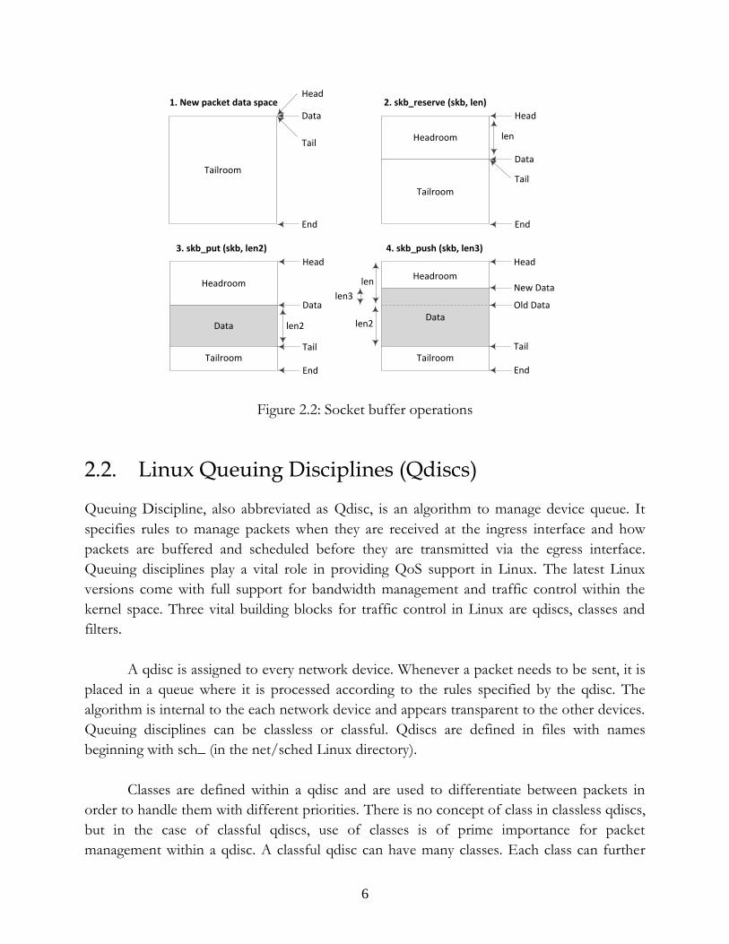
6
Tailroom
Head
Data
Tail
End
Tailroom
Data
Head
Tail
End
len2
Old Data
Tail
End
HeadroomHeadroom
New Datalen
len2
len3
1. New packet data space
3. skb_put (skb, len2) 4. skb_push (skb, len3)
Tailroom
DataData
Head
Tailroom
Headroom
Head
Tail
End
len
2. skb_reserve (skb, len)
Data
Figure 2.2: Socket buffer operations
2.2. Linux Queuing Disciplines (Qdiscs) Queuing Discipline, also abbreviated as Qdisc, is an algorithm to manage device queue. It
specifies rules to manage packets when they are received at the ingress interface and how
packets are buffered and scheduled before they are transmitted via the egress interface.
Queuing disciplines play a vital role in providing QoS support in Linux. The latest Linux
versions come with full support for bandwidth management and traffic control within the
kernel space. Three vital building blocks for traffic control in Linux are qdiscs, classes and
filters.
A qdisc is assigned to every network device. Whenever a packet needs to be sent, it is
placed in a queue where it is processed according to the rules specified by the qdisc. The
algorithm is internal to the each network device and appears transparent to the other devices.
Queuing disciplines can be classless or classful. Qdiscs are defined in files with names
beginning with sch_ (in the net/sched Linux directory).
Classes are defined within a qdisc and are used to differentiate between packets in
order to handle them with different priorities. There is no concept of class in classless qdiscs,
but in the case of classful qdiscs, use of classes is of prime importance for packet
management within a qdisc. A classful qdisc can have many classes. Each class can further

7
have classes, making a parent-child hierarchy that enhances the functionality of a qdisc.
Whenever a class is created, a FIFO qdisc is attached to it by default and when a child class is
added, this qdisc is removed. A class with no child class is called leaf class. Classes are also
defined in files with name beginning with sch_.
Filters are used to allocate outgoing packets to classes within a queuing discipline.
Filters can be applied to qdiscs as well as classes. They classify packets on the bases of
various parameters that are specified when the filter is created. Filters are defined in files with
names beginning with cls_ (in the net/sched Linux directory) [6].
The following figure shows the three basic blocks i.e. qdisc, class and filter for QoS
management in the Linux kernel:-
Class Qdisc
Root Qdisc
Class Qdisc
Filter
Filter
Filter
Figure 2.3: Basic building blocks (qdisc, class & filter) for QoS management [7]
2.2.1. Classless Queuing Disciplines A queuing discipline that accepts packets and only reschedules delays or drops the packets is
considered classless. With classless qdiscs, a simple approach for treatment of packets can be
achieved. If the intent is to lay down a more detailed and complex approach to deal with
packets, Classful qdiscs must be used.
Linux kernel supports different classless qdiscs which are briefly discussed in the
following sections.
8
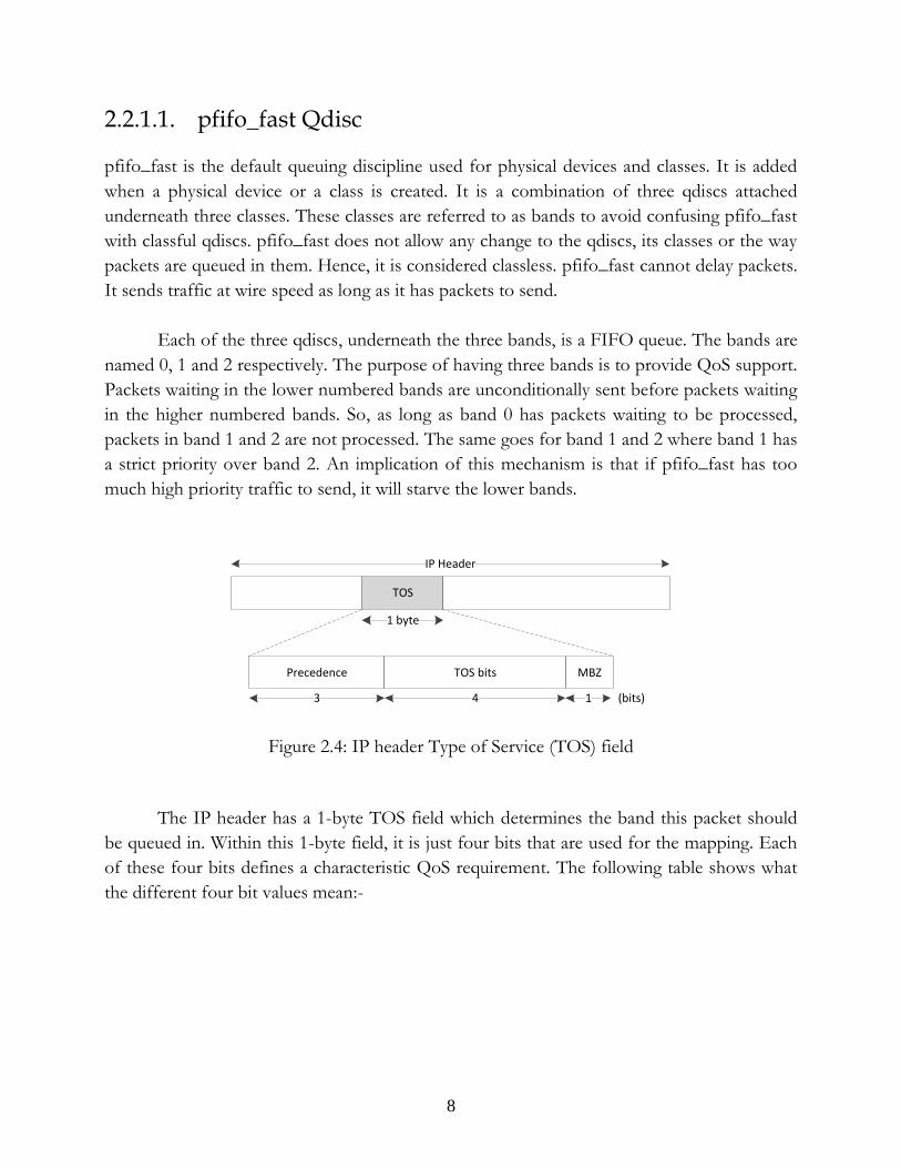
2.2.1.1. pfifo_fast Qdisc pfifo_fast is the default queuing discipline used for physical devices and classes. It is added
when a physical device or a class is created. It is a combination of three qdiscs attached
underneath three classes. These classes are referred to as bands to avoid confusing pfifo_fast
with classful qdiscs. pfifo_fast does not allow any change to the qdiscs, its classes or the way
packets are queued in them. Hence, it is considered classless. pfifo_fast cannot delay packets.
It sends traffic at wire speed as long as it has packets to send.
Each of the three qdiscs, underneath the three bands, is a FIFO queue. The bands are
named 0, 1 and 2 respectively. The purpose of having three bands is to provide QoS support.
Packets waiting in the lower numbered bands are unconditionally sent before packets waiting
in the higher numbered bands. So, as long as band 0 has packets waiting to be processed,
packets in band 1 and 2 are not processed. The same goes for band 1 and 2 where band 1 has
a strict priority over band 2. An implication of this mechanism is that if pfifo_fast has too
much high priority traffic to send, it will starve the lower bands.
TOS
1 byte
IP Header
Precedence MBZTOS bits
3 4 1 (bits)
Figure 2.4: IP header Type of Service (TOS) field
The IP header has a 1-byte TOS field which determines the band this packet should
be queued in. Within this 1-byte field, it is just four bits that are used for the mapping. Each
of these four bits defines a characteristic QoS requirement. The following table shows what
the different four bit values mean:-

9
TOS bits QoS requirement
1000 Minimize delay
0100 Maximize throughput
0010 Maximize reliability
0001 Minimize monetary cost
0000 Normal service
Table 2.1: QoS requirement for TOS bits
The following figure illustrates how packets arriving at the root Qdisc are classified
and enqueued in the different bands, and subsequently dequeued.
Root Qdisc
Class 1 Class 2 Class 3
PFI
FO 0
PFI
FO 1
PFI
FO 2
Packets queued into bands based on ToS bits
Packets always dequeued from band 0 first, then band 1 and lastly band 2
Figure 2.5: Working of pfifo_fast qdisc [10]

10
2.2.1.2. Token Bucket Filter (TBF) Qdisc TBF is a classless queueing discipline for traffic control. It can be used for traffic shaping as
well as controlling the rate of traffic flow.
As the name suggests, it is based on the classical token bucket concept. It consists of
a bucket that is constantly filled by virtual pieces of information, called tokens, at a specified
rate. Each arriving token collects one incoming data packet from the data queue and is then
deleted from the bucket. Packets are queued in a FIFO qdisc and are only sent if the bucket
has tokens available. Each token corresponds to a byte of information. The bucket has a
specified size i.e. the maximum number of tokens it can hold at any instance. This defines the
amount of traffic that can be sent in one go. Tokens arrive at a fixed rate until the bucket is
full [11].
TBF can be tuned to one’s requirements by controlling various knobs e.g. the rate at
which tokens arrive, peak rate which defines the maximum rate at which the bucket gets
emptied, buffer size which defines the amount of data that the qdisc can hold waiting for
tokens to arrive etc. Depending upon the arrival rate of tokens and data packets, the
following scenarios are possible:-
Data arrival rate is equal to the token rate. Each packet gets a token and is sent
without any delay.
Data arrival rate is smaller than the token rate. Each packet gets a token and is sent
without any delay. Unused tokens can be used to send data above the defined token
rate which can cause short data bursts.
Data arrival rate is higher than the token rate. In this case there will be a shortage of
tokens and the qdisc holding packets will get overloaded. Once the qdisc reaches its
maximum holding capacity, incoming packets will be dropped [8].
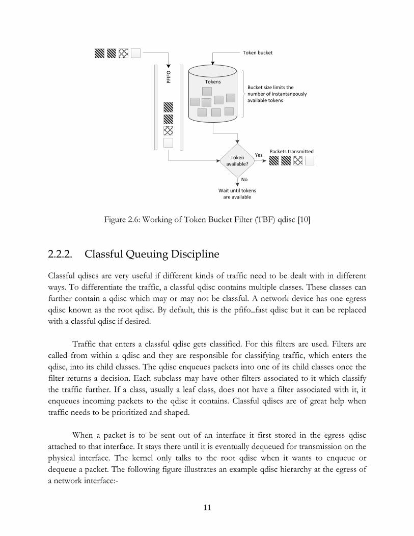
11
TokensPFI
FO
Token available?
Yes
No
Wait until tokens are available
Token bucket
Packets transmitted
Bucket size limits the number of instantaneously available tokens
Figure 2.6: Working of Token Bucket Filter (TBF) qdisc [10]
2.2.2. Classful Queuing Discipline Classful qdiscs are very useful if different kinds of traffic need to be dealt with in different
ways. To differentiate the traffic, a classful qdisc contains multiple classes. These classes can
further contain a qdisc which may or may not be classful. A network device has one egress
qdisc known as the root qdisc. By default, this is the pfifo_fast qdisc but it can be replaced
with a classful qdisc if desired.
Traffic that enters a classful qdisc gets classified. For this filters are used. Filters are
called from within a qdisc and they are responsible for classifying traffic, which enters the
qdisc, into its child classes. The qdisc enqueues packets into one of its child classes once the
filter returns a decision. Each subclass may have other filters associated to it which classify
the traffic further. If a class, usually a leaf class, does not have a filter associated with it, it
enqueues incoming packets to the qdisc it contains. Classful qdiscs are of great help when
traffic needs to be prioritized and shaped.
When a packet is to be sent out of an interface it first stored in the egress qdisc
attached to that interface. It stays there until it is eventually dequeued for transmission on the
physical interface. The kernel only talks to the root qdisc when it wants to enqueue or
dequeue a packet. The following figure illustrates an example qdisc hierarchy at the egress of
a network interface:-
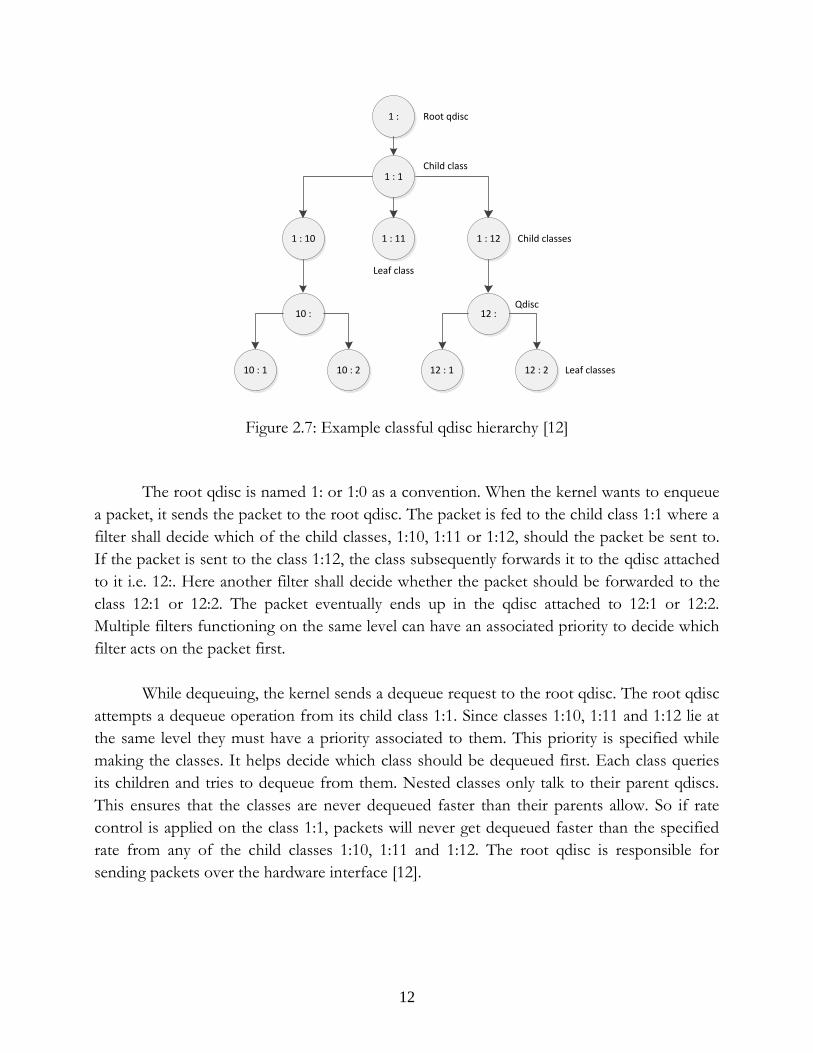
12
1 : Root qdisc
Child class
Child classes
10 : 12 :
Leaf class
Qdisc
Leaf classes
1 : 10 1 : 11 1 : 12
1 : 1
10 : 1 10 : 2 12 : 1 12 : 2
Figure 2.7: Example classful qdisc hierarchy [12]
The root qdisc is named 1: or 1:0 as a convention. When the kernel wants to enqueue
a packet, it sends the packet to the root qdisc. The packet is fed to the child class 1:1 where a
filter shall decide which of the child classes, 1:10, 1:11 or 1:12, should the packet be sent to.
If the packet is sent to the class 1:12, the class subsequently forwards it to the qdisc attached
to it i.e. 12:. Here another filter shall decide whether the packet should be forwarded to the
class 12:1 or 12:2. The packet eventually ends up in the qdisc attached to 12:1 or 12:2.
Multiple filters functioning on the same level can have an associated priority to decide which
filter acts on the packet first.
While dequeuing, the kernel sends a dequeue request to the root qdisc. The root qdisc
attempts a dequeue operation from its child class 1:1. Since classes 1:10, 1:11 and 1:12 lie at
the same level they must have a priority associated to them. This priority is specified while
making the classes. It helps decide which class should be dequeued first. Each class queries
its children and tries to dequeue from them. Nested classes only talk to their parent qdiscs.
This ensures that the classes are never dequeued faster than their parents allow. So if rate
control is applied on the class 1:1, packets will never get dequeued faster than the specified
rate from any of the child classes 1:10, 1:11 and 1:12. The root qdisc is responsible for
sending packets over the hardware interface [12].

13
2.2.2.1. PRIO Qdisc
A PRIO qdisc operates on the same principle as pfifo_fast. But unlike pfifo_fast, it is
classful. It can contain an arbitrary number of classes each having a different priority. When a
PRIO qdisc is created, three classes are automatically created underneath it just like
pfifo_fast. Each of these three classes has its own pfifo qdisc attached to it by default.
Filter
Filter
Filter
Class :1 PFIFO
Class :2 PFIFO
Class :3 PFIFO
PRIO qdisc
Figure 2.8: PRIO qdisc architecture [13]
Like pfifo_fast, PRIO follows the same precedence level in case of the three classes
i.e. a packet is always dequeued from class :1 first. Higher classes are only accessed if the
lower bands do not contain any packet. This qdisc is very useful if packets should be
prioritized not just on the basis of their TOS flags, but also on other factors. Unlike
pfifo_fast, which cannot be modified and has to be used as is, in a PRIO qdisc more siblings
can be added to the three classes available by default. Also, the qdiscs attached to these
classes can be changed from pfifo to other qdiscs [13].
2.2.2.2. Hierarchical Token Bucket (HTB) Qdisc
HTB is a classful shaping qdisc. The underlying principle of its operation relies on a token
bucket just like TBF. Since it is classful, it achieves traffic classification through the use of
filters. Each of the traffic classes can be shaped and scheduled differently. HTB is very
flexible and allows for complex and granular control over traffic through its several knobs.
These knobs allow control of traffic priority, rate of traffic flow, peak rate of traffic flow and

14
size of traffic bursts. It is much simpler to use compared to its predecessor, the CBQ (Class
Based Queueing) qdisc.
Shaping occurs in leaf classes while the inner or root classes only determine how the
available tokens should be distributed amongst the child classes.
Tokens are lent to the child class
HTB qdisc
HTB class
Inner class
Inner class
Leaf class
Leaf class
Leaf class
Rate specified
Figure 2.9: HTB qdisc hierarchy with rate control [14]
Children classes borrow tokens from their parents once they have exceeded their
specified rate and they will do so until the specified peak rate or maximum burst is reached.
At this point incoming packets start getting buffered. The rate defined for the HTB parent
class defines how much practical amount of bandwidth is available [14].
2.3. MPLS Transport Profile (MPLS-TP)
Before MPLS, carrier networks employed an overlay model with SDH/SONET at layer 1
while ATM at layer 2. With the advent of MPLS, it became very popular with service
providers due to the flexibility and attractive features it offers. MPLS is a connection-
oriented packet transport networking technology which provides features like sophisticated
traffic engineering options, scalable IP VPNs, layer 2 transport, QoS support and efficient
bandwidth utilization through bandwidth reservation and borrowing. But MPLS lacked
15
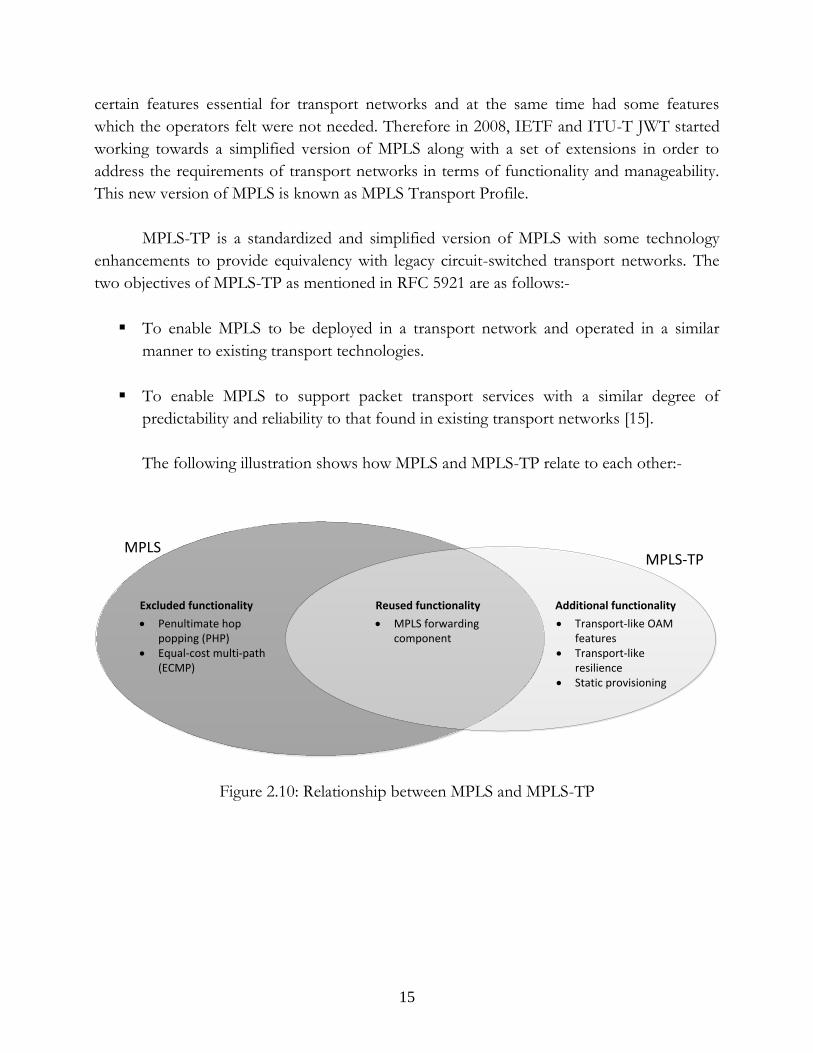
certain features essential for transport networks and at the same time had some features
which the operators felt were not needed. Therefore in 2008, IETF and ITU-T JWT started
working towards a simplified version of MPLS along with a set of extensions in order to
address the requirements of transport networks in terms of functionality and manageability.
This new version of MPLS is known as MPLS Transport Profile.
MPLS-TP is a standardized and simplified version of MPLS with some technology
enhancements to provide equivalency with legacy circuit-switched transport networks. The
two objectives of MPLS-TP as mentioned in RFC 5921 are as follows:-
To enable MPLS to be deployed in a transport network and operated in a similar
manner to existing transport technologies.
To enable MPLS to support packet transport services with a similar degree of
predictability and reliability to that found in existing transport networks [15].
The following illustration shows how MPLS and MPLS-TP relate to each other:-
MPLSMPLS-TP
Additional functionalityReused functionalityExcluded functionality
· MPLS forwarding component
· Penultimate hop popping (PHP)
· Equal-cost multi-path (ECMP)
· Transport-like OAM features
· Transport-like resilience
· Static provisioning
Figure 2.10: Relationship between MPLS and MPLS-TP
16
MPLS-TP inherits the MPLS forwarding plane i.e. packets are label switched just as in
MPLS. It also offers additional functionality to specifically address the requirements of
transport networks. This added functionality includes:-
Transport-like OAM functions
Transport-like operations
Transport-like resilience mechanisms
Legacy transport networks use numerous tools to monitor and manage the network
so that they conform to the SLAs. Providing OAM functions that enable monitoring and
managing the network was a key objective with MPLS-TP. MPLS-TP provides various OAM
functions that include the ability to send in-band OAM messages, performance monitoring
(e.g. delay measurement and loss measurement) and fault detection.
OAM messages use in-band control channels i.e. the OAM messages to monitor an
LSP travel along with the traffic packets through the same LSP. To differentiate OAM
packets from other packets, an additional header called the Generic Ach (G-ACh) header is
used. This header tells the receiving end node of an LSP that the packet should be handled
by an OAM packet handler function. A G-Ach PDU is encapsulated in an MPLS header
where the label value used is 13. This value was assigned by IANA and is reserved for G-
ACh label [16].
MPLS-TP offers rapid fault detection OAM functions through extended Bidirectional
Forwarding Detection (BFD). For this BFD Continuity Check (CC) messages are used.
With MPLS, control plane mechanisms can be used to establish LSPs across the
MPLS network. MPLS uses protocols such as OSPF-TE, RSVP-TE, LDP and BGP for
control plane signaling. Transport networks, however, usually employ a static control plane.
Communication paths are provisioned manually through a NMS. Therefore static
provisioning was the main focus with MPLS-TP. NMS-driven control plane allows operators
to configure and manage their networks in the same way as the legacy circuit-switched
networks were managed. It is important to note here that MPLS-TP also allows for
provisioning through a dynamic control plane. This can have its own advantages especially in
terms of scaling. If an operator wants to employ a dynamic control plane, it can use GMPLS
to setup LSPs to operate with MPLS-TP.
One of the two main objectives of MPLS-TP was to provide resilience mechanisms
similar to that of legacy transport networks. Though MPLS provides a rich set of protection

17
mechanisms like MPLS Fast Reroute, MPLS Global Path Restoration and MPLS Global Path
Protection, MPLS-TP further enhances the resiliency mechanisms of MPLS by adding
support for sub-50 ms OAM-triggered protection. This is the key to the solution that this
thesis provides because OAM-triggered protection allows switching an LSP to its secondary
path. MPLS Fast Reroute offers protection in ring topologies but in an inefficient way as
secondary paths are not optimal. MPLS-TP offers ring protection mechanisms with
optimizations such as wrapping and steering to ensure that the secondary paths are optimal.
MPLS-TP also offers linear protection mechanisms which provide a solution to the load
balancing ambition of this thesis [15].
Some the features of MPLS have been turned off in MPLS-TP. Turning off some
features helps in reducing network operational complexity and at the same time adding OAM
enhancements and functionality provides better network performance monitoring, fault
management and protection switching capabilities [17].
2.3.1. MPLS-TP Linear Protection
Linear protection is a recovery mechanism in MPLS-TP that offers simple and rapid
protection switching. It provides an alternate data path between any pair of nodes in a mesh
network. With MPLS-TP linear protection, an LSP or a group of LSPs traversing a specified
set of links between two nodes can be protected end-to-end by another link diverse LSP or a
group of LSPs between the same nodes. Resources for the protection LSPs, which primarily
include bandwidth, are allocated beforehand.
If a link or node on the working path fails, end nodes are notified and traffic is
immediately switched to the protection LSPs. With MPLS-TP linear protection the switching
time is within 50 ms. The end points can be configured to work in revertive mode so that the
traffic flow is shifted back to the working path once it is up and running. MPLS-TP linear
protection offers different protection architectures such as 1+1, 1:1 and 1:n. The protection
architectures are briefly described as follows:-
1+1 protection: Traffic is sent on both the working and protection path at the source.
At the sink, a selector is used to receive traffic either from the working path or the
protection path.

18
Intermediate Node
Local End Far End
Working path
Protection path
Selector
Traffic is sent on working & protection paths simultaneously
Figure 2.11: MPLS-TP linear protection 1+1 architecture
1:N protection: N working paths are protected using one protection path. Under
normal circumstances traffic is sent on the working paths. The protection path is used
to send traffic only if a working path fails.
1:1 protection: It is a special case of 1:N protection where one working path can be
protected using a protection path [18].
Intermediate Node
Local End Far End
Working path
Protection path
Selector
Traffic is sent on either working or protection path
Figure 2.12: MPLS-TP linear protection 1:1 architecture
If there is a fault on a physical link/node on the working path or if one of the many
LSPs traversing the working path fails, traffic is switched to the corresponding protection
LSP. The switching process happens in two phases mentioned as follows:-
Detecting failure on the working path
Switching traffic to the protection path

19
Each of the two phases is achieved using different protocols. A fault is detected using
Connectivity Check (CC) messages of the Bidirectional Forwarding Detection (BFD)
protocol. Once the fault is detected, a protocol called Protection State Coordination (PSC) is
used to switch traffic to the protection path.
2.3.1.1. Bidirectional Forwarding Detection (BFD) Protocol
Being able to rapidly detect communication failures between two systems is very important
for carrier networks since they carry huge amounts of data on which several customers rely.
The faster a fault on a communication path is detected, the faster an alternative path can be
established. Fault detection mechanisms offered by some link layer protocols e.g. SONET
are very rapid. But there are other protocols, like Ethernet, which do not offer such signaling.
With such protocols, networks use “Hello” mechanisms, often provided by routing
protocols, to detect failures. The fault detection times of these “Hello” mechanisms,
however, are no better than a second which is far too long for networks carrying data at
gigabit rates.
Bidirectional Forwarding Detection enables low-overhead short-duration failure
detection between two forwarding engines. BFD sessions are configured between a pair of
nodes through which both the nodes exchange BFD messages periodically to monitor the
communication path which can be a physical path, virtual circuit, tunnel or an MPLS LSP.
With BFD the failure detection time is in the order of tens of milliseconds. BFD sessions are
point-to-point and unicast. So, for a bidirectional communication path e.g. a bidirectional
LSP, two BFD sessions must be configured, one in each direction. BFD can operate over
any media, at any protocol layer.
As mentioned earlier, MPLS-TP employs in-band OAM messages to monitor an LSP.
To realize a control channel associated to an MPLS LSP, a G-ACh header is used. The OAM
messages are encapsulated in a G-ACh header to differentiate them from other packets. The
existence of a G-ACh header is agreed upon during control plane signaling to establish the
LSP. When static provisioning is used, there must be a way to know that the data is
encapsulated in a G-ACh header. In order to identify the presence of a G-ACh header, a G-
ACh label (GAL) is used. It informs an LSR that a packet it receives on an LSP belongs to an
associated control channel (ACh). GAL is an MPLS reserved label with value 13. Every G-
ACh PDU is encapsulated in an MPLS header with label value 13. GAL must always be at
the bottom of the label stack, so the Bottom of Stack bit (S bit) of the MPLS header is always
20
1. A receiving LSR must not forward a G-ACh packet to another node based on the GAL
label [16].
MPLS-TP LSPs, emulating traditional transport circuits, need to provide a Continuity
Check function to detect the Loss of Continuity (LOC) defect between two nodes. This is
achieved through a BFD extension for Continuity Check (CC) messages. GAL/G-ACh
encapsulation is used for these BFD messages [19].
Continuity Check (CC) messages are used to check the liveliness of a communication
path or an LSP. These are periodic messages exchanged between two end nodes which help
both the nodes monitor the state of the link. If at any point, one of the two nodes stops
receiving CC messages, it infers that the link has broken down. It is important to note here
that these BFD CC messages are sent as in-band OAM messages in an LSP. Hence, these CC
messages allow monitoring a Label Switched Path independently.
When a BFD session is configured, a number of parameters are defined. Two of these
parameters are:-
1. Transmit interval: Defines the time interval after which successive CC messages are
sent.
2. Detect multiplier: Number of consecutive drops of CC messages before the receiving
end node infers that the LSP is broken.
Values for these parameters are carried in the BFD control packet. Based on these
two values, the fault detection time is:-
Fault detection time = Remote TX interval × Detect multiplier
2.3.1.2. Protection State Coordination (PSC) Protocol
PSC is a protocol that is used to help coordinate between both ends of a protection domain
in selecting the proper traffic flow. In the 1:1 MPLS-TP linear protection architecture, a
protection LSP is dedicated to a working LSP. Traffic is transmitted on either the working or
the protection path by using a selector at the source of the protection domain. Similarly, at
the sink of the protection domain a selector is used to select the path that carries normal
traffic. Since the source and sink need to be coordinated to ensure that the selector at both
ends selects the same path, the 1:1 architecture employs the PSC protocol. Coordination is
even more important when employing bidirectional co-routed LSPs since there is a need to

21
verify that traffic continues to be transported on the path that both end nodes deem
functional.
Both ends of a protection domain use PSC to determine when traffic needs to be
shifted to or from the working or protection path. Protection switching can be triggered on
the basis of updates received from either the far end LER or generated at the local node.
Both ends of a protection domain run the Protection State Control logic. The Protection
State Control logic is illustrated in the following figure:-
Local Request Logic
OAM indication
Server indication
Control plane indication
Operator command
PSC Control Logic
Highest local request
Remote PSC request
Message Generator Output PSC message
WTR timerWTR expires
Start/Stop
Action
Figure 2.13: Protection State Control Logic
Protection State Control logic processes inputs generated locally as well as inputs
received from the far-end LER. Based on these inputs, the LER performs certain actions e.g.
switching the selector to transmit on the working or protection path, switching the selector
to receive on the working or protection path, transmit different protocol messages etc. The
local request logic takes inputs from the OAM layer, server layer, control plane and operator
commands. Every local request has an associated priority. The local request logic selects the
highest priority local request and passes it on to the PSC control logic which cross-checks it
with the information received from the far-end LER. Based on these two inputs the PSC
control logic determines the actions that need to be taken. These actions include actions
taken locally, messages sent to the far-end LER and updating the state of the protection
domain.

22
Local request logic receives input from different sources which are briefly discussed
as follows:-
OAM gears like BFD (CC, CV, and RDI) messages are used to detect failures or
service degradation on the working path. Any update triggered is fed to the local
request logic.
Server layer of the network detects failure conditions at the underlying layer and may
issue an indication to the MPLS-TP layer. The server layer can have its own
protection mechanism, and therefore, this input may be controlled by a hold-off
timer.
Control plane indications in the network, like signaling or routing, can also trigger
protection switching. Updates triggered by control plane are fed to the local request
logic. MPLS-TP control plane is either static or dynamic. Static control plane is based
on NMS provisioning while dynamic control plane for MPLS-TP LSPs is based on
GMPLS.
Operator commands can be issued manually in order to trigger protection switching.
These commands may include clear command, forced switch-over, manual switch-
over or lockout of protection.
Wait to Restore (WTR) time is the time it takes to recover back to the working path
from the protection path when the fault is restored. The WTR timer generates a
request when its period expires. WTR works in revertive mode of protection.
The PSC Control Logic processes the following three inputs:-
1. Current local request output from the local request logic.
2. Remote request message from the remote end.
3. The current state of PSC control logic (maintained internally).
Based on these three inputs, the PSC control logic determines the new state of the
protection domain, the actions that need to be taken and any messages that should be
generated for delivery to the remote end. These actions include switching traffic to or from
the working or protection path. Both the end nodes are informed before switching over
traffic to the working or protection path through PSC messages.
23
PSC is a single phased protocol meaning that each end node notifies its pairing node
before protection switching and switches over the traffic without receiving any
acknowledgement. PSC control packets are always sent over the protection path. This is so
that in case of a failure on the working path, PSC messages are not affected.
Whenever the protection state changes because of a local or a remote request, three
PSC messages are sent immediately in order to perform rapid protection switching. Three
messages are sent to ensure that at least one of them is received in case of packet loss. These
three messages are sent within 3.3 ms to have fast protection switching (within 50 ms). After
these three messages, PSC messages are sent periodically at intervals of 5 seconds and are
used to check the liveliness of the PSC session. If no valid PSC message is received during
several continual message time intervals, the last valid PSC message is pertinent [18].
2.4. Related Work
ITU-T Recommendation G.808.1 (Generic Protection Switching – Linear Trail and
Subnetwork Protection) defines functional models and characteristics of various linear
protection schemes for circuit-switched connection-oriented networks such as SDH and
ATM networks. It discusses two protection schemes namely Trail Protection and
Subnetwork Connection Protection. The two protection schemes are briefly described in the
following subsections.
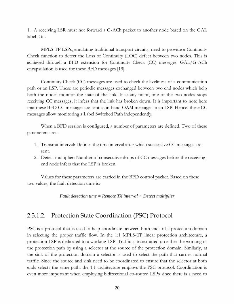
2.4.1. Trail Protection
This protection scheme provides protection for an entire trail across an operator’s network
or multiple operators’ networks. In other words, it provides dedicated end-to-end protection
in different network architectures such as mesh and ring networks. The path along which it
provides protection can have several network elements. In fact, theoretically there is no limit
on the number of network elements in the protected trail.
24
Protectionswitchingfunction
Networkelements
Working transport entity
Protection transport entity
Figure 2.14: Trail Protection [23]
MPLS-TP linear protection is based on the trail protection concept. Protected trails
are monitored using signals like the CC messages. If a fault occurs on the working transport
entity, an Alarm Signal Indication (AIS) is raised. The protection switching functions at both
ends then wait for a defined period of time before switching. If a CC message is received in
this period, the AIS defect condition is cleared.
Trail protection has two functional models namely Individual Trail Protection i.e. 1:1 or
1+1 protection and Group Trail Protection i.e. 1:n protection [23].
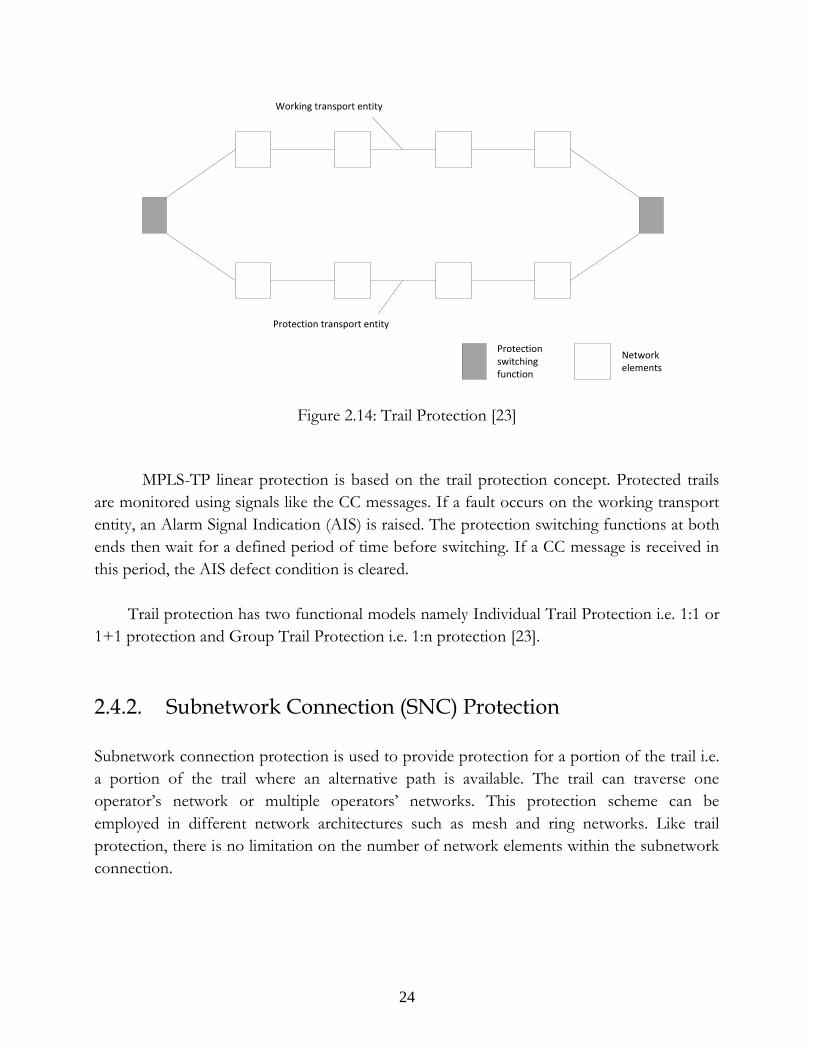
2.4.2. Subnetwork Connection (SNC) Protection
Subnetwork connection protection is used to provide protection for a portion of the trail i.e.
a portion of the trail where an alternative path is available. The trail can traverse one
operator’s network or multiple operators’ networks. This protection scheme can be
employed in different network architectures such as mesh and ring networks. Like trail
protection, there is no limitation on the number of network elements within the subnetwork
connection.

25
SNC protection can support network architectures that make use of cascaded
protected subnetworks. A subnetwork can therefore restore faults without affecting other
subnetworks. This makes the system more robust compared to trail protection.
Protectionswitchingfunction
Networkelements
Protected domain 1 Protected domain 2
Working transport entities
Protection transport entities
Figure 2.15: Cascaded SNC Protection [23]
Like trail protection, SNC protection also has the individual and group functional
models. SNC should not be confused with MPLS FRR. SNC can provide protection over
multiple links and nodes within one subnetwork whereas MPLS FRR provides protection
strictly for one link or node [23].
2.4.3. Service protection in Dynamic Bandwidth Networks (DBNs)
Amendment 2 to ITU-T recommendation G.808.1 adds appendix VII (Solution for service
protection in DBN) to the recommendation. It proposes a solution for service protection
switching in DBNs. Bandwidth of the links in DBNs is dynamic in the sense that network
elements adjust the transmission rate in real time to suit the current propagation conditions.
When a link suffers from bandwidth degradation, so that the available bandwidth is less than
that under normal conditions, some services associated with that link could no longer be
supported. Therefore, these services can be switched to alternate communication paths. This
solution facilitates service-level load sharing in DBNs, ensuring protection for high priority
services while maintaining high network utilization.

26
Service A Service A
X Y
Service B Service B
Link XY
Protected domain
Protectionswitchingfunction
Networkelements
Figure 2.16: Service protection in DBNs [24]
In figure 2.16 network elements X and Y implement a dynamic bandwidth link XY.
The transmission rate on this link is adapted to the propagation conditions. This functionality
is taken care of at layer 1. Therefore, network elements X and Y have access to the current
dynamic bandwidth for link XY. How this information is generated is not in the scope of this
recommendation.
Each service is associated with a Committed Information Rate (CIR). The CIR for
service A and B will be referred to as CIR A and CIR B. Protection actions are triggered
based on Signal Degrade (SD) messages which are generated when network elements X and
Y detect bandwidth degradation on link XY.
Events that occur starting from signal degradation to protection action are based on
whether network elements X and Y have knowledge of service bandwidths CIR A and CIR
B. In the case where they have this knowledge, if the aggregated CIR (CIR A + CIR B) is less
than the current link bandwidth of XY no signal is generated by network elements X and Y.
If the link bandwidth is degraded to the extent that only the higher priority service can be

27
sustained, an SD message is sent to the lower priority service protection switching function.
If the current bandwidth degrades to the extent that the CIR of the higher priority service
cannot be met, SD messages are sent to the protection switching functions of both service A
and service B.
In the case where network elements X and Y have no knowledge of service
bandwidths CIR A and CIR B, SD messages which carry current bandwidth information are
signaled to the head-ends. The head-ends will subsequently update their distribution policy
based on the received bandwidth information. If multiple degradations occur and the head-
ends receive multiple bandwidth values, the lowest value is selected. The head-end will
perform protection switching based on the updated distribution policy [24].

28
Chapter 3
Design
This chapter discusses the proposed solution to the problem described in Section 1.2. It also
describes in detail how the solution was implemented to form a complete system as a proof
of concept.
3.1. Load Balancing Mechanism
The idea that this thesis presents to load balance traffic in a microwave network is based on
having disjoint predesignated primary and secondary communication paths in the network.
Traffic will be switched to the secondary path if a microwave link on the primary path
experiences bandwidth degradation due to unfavorable weather conditions. When switching
traffic, only enough traffic must be switched to the secondary path that the troubled
microwave link is able to handle the remaining traffic. To do this, a granular control of traffic
on the working path is needed.
The following figure shows a typical ring topology which is commonly used in
transport networks of service providers:-
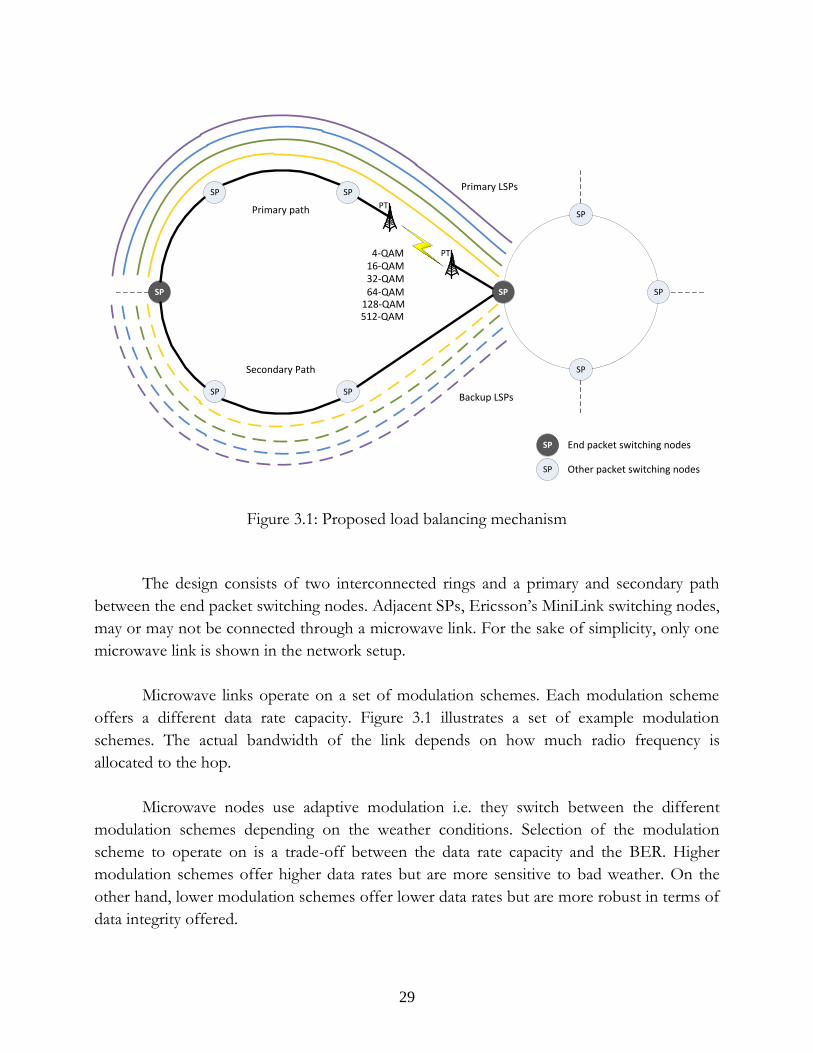
29
SP
SP
SP SP
SP
SP
SP
SP
SP
PT
PT
Primary LSPs
Backup LSPs
4-QAM16-QAM32-QAM64-QAM
128-QAM512-QAM
SP
SP
End packet switching nodes
Other packet switching nodes
Primary path
Secondary Path
Figure 3.1: Proposed load balancing mechanism
The design consists of two interconnected rings and a primary and secondary path
between the end packet switching nodes. Adjacent SPs, Ericsson’s MiniLink switching nodes,
may or may not be connected through a microwave link. For the sake of simplicity, only one
microwave link is shown in the network setup.
Microwave links operate on a set of modulation schemes. Each modulation scheme
offers a different data rate capacity. Figure 3.1 illustrates a set of example modulation
schemes. The actual bandwidth of the link depends on how much radio frequency is
allocated to the hop.
Microwave nodes use adaptive modulation i.e. they switch between the different
modulation schemes depending on the weather conditions. Selection of the modulation
scheme to operate on is a trade-off between the data rate capacity and the BER. Higher
modulation schemes offer higher data rates but are more sensitive to bad weather. On the
other hand, lower modulation schemes offer lower data rates but are more robust in terms of
data integrity offered.

30
The entire load balancing process is a series of two steps mentioned as follows:-
1. Rate limiting traffic at the SP, which precedes the microwave link, to prevent
congestion on the microwave link.
2. Switching traffic from the primary path to the secondary path.
3.1.1. Rate Limiting Traffic at the SP
To avoid congestion on a troubled microwave link, a reactive approach is employed. This
involves the use of a radio condition signaling mechanism implemented as part of the driver
of the Ericsson proprietary network interfaces that connect the SP and the PT. When the
microwave link experiences service degradation, there is a need to inform the sending packet
switching node about the current link condition so that it can rate limit traffic. As soon as the
microwave link adapts to a lower modulation scheme, the PT informs the SP about the
current radio conditions and the SP limits the transmission rate accordingly. This does not
eliminate the problem completely because traffic may still be incident at the SP from the
backbone network at a higher rate. Therefore, some or all of the traffic should be switched to
the secondary path.
3.1.2. Switching Traffic
The load balancing idea, presented in this thesis, is based on having multiple virtual paths
established on the primary communication path and corresponding backup virtual paths
established on the secondary communication path. Figure 3.1 illustrates four pairs of working
and backup LSPs established along the primary and secondary path respectively. The key lies
in having independent control of each virtual path and having the ability to switch traffic on
a virtual path to its backup virtual path on the secondary communication path. To do this
MPLS-TP linear protection is employed.
MPLS-TP offers the facility of sending in-band OAM messages through the
established Label-Switched Paths (LSPs) to monitor them. The OAM messages, used to
check the liveliness of an LSP, are the BFD Continuity Check (CC) messages. To switch
traffic from an LSP to its backup LSP, the BFD CC messages of that LSP are discontinued.
Consequently, the end SPs coordinate with each other using the PSC protocol and switch
traffic to the backup LSP. If later, the microwave link conditions improve and the transmit
rate of the SP is increased, the discontinued CC messages can be allowed to pass again. This

31
will cause the end SPs to synchronize using PSC messages and switch traffic from the backup
LSP to the primary LSP.
The decision to switch traffic from the primary path to the secondary path must be
made at some point. This decision is made by monitoring the state of the transmit buffer at
the SP i.e. the transmit buffer of the EPI. If the queue length of the transmit buffer starts
increasing, the SP infers that there is a need to switch traffic to the protection path.
Subsequently, it terminates an LSP by discontinuing the CC messages. If that is not enough,
another LSP is terminated. The SP keeps terminating LSPs on the primary path until the
queue length of its transmit buffer stops increasing. The state of the buffer must be
correlated to the state of the microwave link i.e. it should be ensured that the buffer build up
is due to a recent decrease in bandwidth.
3.1.3. Load Balancing Scenario
The following series of figures illustrates a scenario where different radio condition control
messages are generated when the weather varies. As a result, LSPs are switched to and from
the primary and secondary path to load balance traffic.
SP
SP
SP SP
SP
SP
SP
SP
SP
PT
PT
Primary LSPs
512-QAM
1
Figure 3.2: Load balancing scenario (a) - Good weather conditions, microwave link operates
at 512-QAM. The traffic of all four LSPs is supported on the primary path.

32
SP
SP
SP SP
SP
SP
SP
SP
SP
PT
PT
Primary LSPs
128-QAM
Drop BFDpackets
Radio condition control frame
Backup LSPs
2
Figure 3.3: Load balancing scenario (b) - Weather conditions deteriorate, microwave link
adapts to 128-QAM. A radio condition control packet is generated. The traffic of four LSPs cannot be supported on the primary path now. BFD CC packets of one LSP are
discontinued and it switches to the secondary path.
SP
SP
SP SP
SP
SP
SP
SP
SP
PT
PT
Primary LSPs
64-QAM
Drop BFDpackets
Radio condition control frame
Backup LSPs
3
Figure 3.4: Load balancing scenario (c) - Weather conditions deteriorate further, microwave link adapts to 64-QAM. A radio condition control packet is generated. The traffic of three LSPs cannot be supported on the primary path now. So, another LSP is switched to the
secondary path.

33
SP
SP
SP SP
SP
SP
SP
SP
SP
PT
PT
Primary LSPs
512-QAM
Radio condition control frame
4
Figure 3.5: Load balancing scenario (d) - Weather conditions go back to normal, microwave
link adapts to 512-QAM once again. A radio condition control packet is generated. All terminated BFD sessions are restored. All four LSPs are supported on the primary path
again.
3.2. Realizing the Ericsson Proprietary Interface (EPI)
To implement and demonstrate the load balancing idea proposed in this thesis, a prerequisite
was to code the driver of an EPI. This interface connects Ericsson’s MiniLink PT node, a
microwave node, and any network forwarding device such as Ericsson’s MiniLink SP node.
The driver implements an Ericsson proprietary protocol which rides over the Ethernet layer.
As part of the thesis project, the specifications for this protocol were studied and
implemented. These specifications primarily define how data should be handled and
encapsulated.
The protocol internals also include a radio condition signaling mechanism which is of
prime importance with regard to the goal of this project. This mechanism was implemented
as part of the driver for the EPI. The driver is installed at the PT as well as the SP. The
mechanism is used by the PT to inform the SP of the microwave link condition. Radio
condition control frames are generated by the PT towards the SP whenever there is a change
in the state of a microwave link. Through the control frames it is possible to deduce how
much traffic can be accommodated over the air interface. This helps prevent congestion and
hence data loss on the microwave link.

34
The following figure illustrates how the Ericsson proprietary interface (EPI) was realized:-
Driver1 code
SP
ZebOS Routing Stack
Driver1 code
SP
ZebOS Routing Stack
PT
Driver1 code
PT
Driver1 code
Microwave Link
eth0 eth0
eth1 eth1
Virtual Interface
Virtual Interface
Packet buffer Packet buffer
Tx buffer Tx buffer
1 – Driver for the Ericsson proprietary interface
Figure 3.6: Realizing the Ericsson proprietary interface (EPI)
To develop the SP and PT with the EPI driver and the load balancing functionality,
Linux-based servers were used. The load balancing idea proposed in this thesis involves the
use of MPLS-TP LSPs. Data is passed in LSPs established along the primary and secondary
communication paths. To provide the MPLS label switching functionality, the ZebOS
routing stack was used. The MPLS kernel module provided by ZebOS was patched into the
Linux kernel. The patched Linux kernel was then compiled and installed on the servers that
represent the SP. The routing stack was then configured using ZebOS user space daemons to
define the label operations and the ingress/egress labels.
Data is received by the SP on its eth0 interface from its preceding node. This data
contains MPLS packets. The ZebOS routing stack looks up its MPLS forwarding table and
determines the outgoing label and interface of the packet. The outgoing interface is a virtual
interface which represents the EPI. This virtual interface is created in the Linux kernel and is
a customized version of the Ethernet interface. This is because the EPI rides on the Ethernet
layer. It is important to notice that the ZebOS routing stacks deployed in the SPs see each
other directly through the virtual interface or the EPI. What happens in between is not
known to them. This means that the Ethernet header of packets queued by the ZebOS
routing stack in the EPI, contains the destination MAC address of the EPI of the following
SP.
Packets queued in to the transmit buffer of the EPI are dequeued when the kernel is
ready to transmit them. They are subsequently handled by the hard_start_xmit function

35
implemented in the driver of the EPI. The hard_start_xmit function makes the necessary
changes before queuing the packet into the transmit buffer of the eth1 interface using the
dev_queue_xmit() function. These changes accommodate the standards defined in the
specifications of the EPI. The Ethernet header of packets, queued for transmission in the
eth1 transmit buffer, contain the destination MAC address of the following PT.
The following figure illustrates how a frame looks like on the wire that connects an SP
and a PT:-
Ethernet header
Ericsson proprietary
interface header
Ethernet header
Payload
Belongs to eth1Added by the Ericsson
proprietary interface driverBelongs to the
virtual interface
Figure 3.7: Frame format on the wire that connects the SP and PT
When received at the PT, the handler function for the EPI is called. This function is
defined for the Ethertype of the Ericsson proprietary protocol using the function
dev_add_pack() and the struct packet_type. dev_add_pack() is used to add a protocol
handler to the networking stack. The struct packet_type defines the Ethertype of a protocol
and the handler function for packets belonging to that Ethertype.
The PT performs header de-encapsulations on the received frames and transmits the
packet on the microwave link as the standards dictate.
3.3. MPLS-TP Linear Protection vs. MPLS-TE Protection Mechanisms
Service providers all over the world have switched over from legacy technologies like
ATM/SDH/SONET to IP/MPLS in order to provide data transport services. MPLS uses
routing functionality of underlying layer 3 routing protocols to set up label switched paths
(LSPs). It is a highly scalable; protocol agnostic, data carrying mechanism. IP/MPLS layer
does not have visibility of the entire network layout by default. It relies on the underlying
36
IGP protocol for best path selection and network visibility. IGP operates using LSAs to
update the state of nodes in a network.
IP routing protocols typically have convergence times of the order of a few seconds.
It can be improved up to one or two seconds using certain enhancements like fast SPF and
LSA propagation triggering, priority flooding, fast fault detection etc. It may be sufficient for
some traffic but there are many services that are critically delay dependent like voice traffic
where delays cannot exceed 50 ms. Therefore, other mechanisms are needed to improve
convergence time and achieve rapid switching for delay dependent traffic.
MPLS has an important feature of Traffic Engineering (TE) which is useful in
optimizing the allocation of network resources and steering the traffic flow in a network.
This results in efficient resource utilization and CAPEX/OPEX savings as compared to
legacy technologies. Besides routing and improved QoS, protection/restoration mechanisms
are of key importance for a service provider as networks are prone to faults and service
degradation. IP/MPLS has robust mechanisms to provide resiliency and network availability.
In case of a failure on a link or node in a protected LSP, the fault is detected and traffic is
switched to an alternate path.
Mechanisms used for network resiliency are categorized into protection mechanisms
or restoration mechanisms. Protection and restoration are defined as follows:-
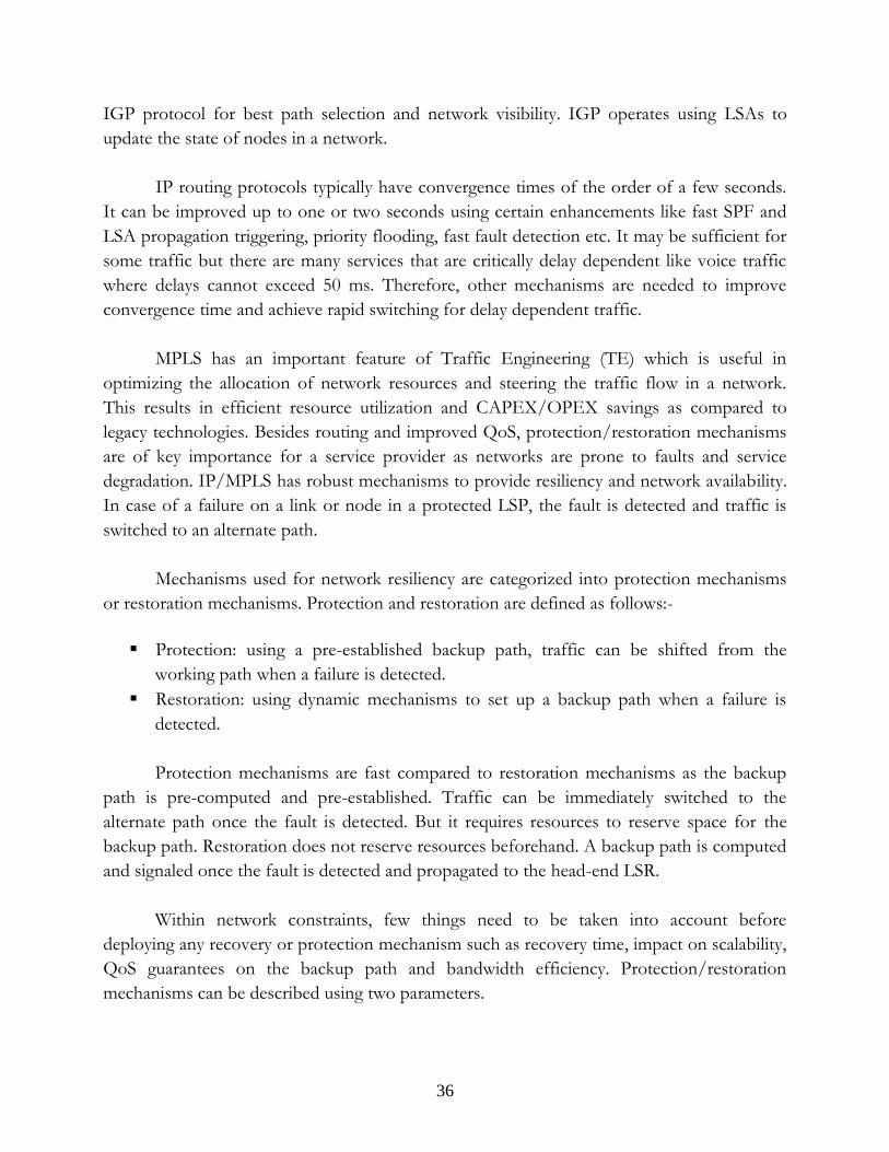
Protection: using a pre-established backup path, traffic can be shifted from the
working path when a failure is detected.
Restoration: using dynamic mechanisms to set up a backup path when a failure is
detected.
Protection mechanisms are fast compared to restoration mechanisms as the backup
path is pre-computed and pre-established. Traffic can be immediately switched to the
alternate path once the fault is detected. But it requires resources to reserve space for the
backup path. Restoration does not reserve resources beforehand. A backup path is computed
and signaled once the fault is detected and propagated to the head-end LSR.
Within network constraints, few things need to be taken into account before
deploying any recovery or protection mechanism such as recovery time, impact on scalability,
QoS guarantees on the backup path and bandwidth efficiency. Protection/restoration
mechanisms can be described using two parameters.

37
Fault detection time
Protection switching time
Fault detection time is the time it takes to detect a fault and inform the upstream
head-end LSR about it. This time is important because in order to minimize the outage time,
the head-end LSR should be informed if a fault has occurred on the working path as soon as
possible. Based on the information received, the head-end LSR triggers protection switching.
Protection schemes in IP/MPLS can be broadly categorized as follows:-
MPLS-TE Global Path Restoration
MPLS-TE Global Path Protection
MPLS-TE Local Protection (Fast Reroute)
These mechanisms differ based on signaling aspects with regard to fault detection and
backup path computation. All the above mentioned schemes can be employed based on the
service requirements and limitations in a network.
MPLS transport profile (MPLS-TP) is an extension of IP/MPLS with additional
OAM features and resiliency mechanisms for transport networks. It has an important feature
called MPLS-TP linear protection. MPLS-TP linear protection and the
protection/restoration mechanisms provided by IP/MPLS are discussed and compared in
the following sections. The discussion will revolve around the fault detection time and the
mechanism to trigger traffic switching.
3.3.1. MPLS-TE Global Path Restoration
Recovery, after a fault occurs, involves coordination and potential synchronization between
network elements. Recovery time is the time between fault occurrence and recovery. MPLS-
TE global restoration is the default resiliency mechanism provided by MPLS-TE. When a
failure is detected along a LSP, it is propagated to the upstream head-end LSR using a FIS
message. The failure is detected through either the underlying layer 2 protocol or IGP hello
messages that are sent periodically to monitor the state of the link. The FIS message is either
an IGP LSA update informing the head-end LSR of a topology change, or it is an RSVP Path
Error (PathErr) message. The time it takes for an FIS to reach the head-end LSR largely
depends on IGP tuning.

38
The failure is propagated using LSAs and can take considerable time as all nodes need
to synchronize and update their forwarding table when LSAs are received. Once the FIS is
received at the head-end LSR, it computes a new path, on the fly, and signals a TE LSP along
that path. MPLS-TE uses Constrained Shortest Path Forwarding (CSPF) which is an
extension of the Shortest Path Forwarding (SPF) protocol for recalculating the path
dynamically based on the available resources. CSPF uses classic shortest path algorithms
using link state updates. The restoration time can be of the order of a few seconds.
Global path restoration is the slowest recovery mechanism compared to other MPLS-
TE protection mechanisms. This is because it requires an FIS to be propagated to the head-
end LSR, dynamic path computation (which grows with the network complexity) and TE
LSP signaling. Global path restoration cannot provide recovery times on the order of tens of
milliseconds [21].
3.3.2. MPLS-TE Global Path Protection
MPLS-TE global path protection is a repair mechanism where a diversely routed backup TE
LSP is computed and signaled for each primary TE LSP before any failure. When a failure is
detected, an FIS message is sent to the head-end LSR and traffic is immediately switched
onto the backup LSP. No backup path computation or signaling of the new LSP is required.
In this way the recovery time is minimized. Global path protection triggers protection
switching faster than global path restoration.
Like global path restoration, global path protection also requires an FIS to be
propagated to the head-end LSR. But traffic switching in global path protection is faster
since the backup path is pre-established. MPLS-TE global path protection cannot in most
cases provide tens of milliseconds of recovery time which might be an issue for delay
sensitive traffic like voice and for large carrier networks carrying data at gigabit rates [21].
3.3.3. MPLS-TE Local Protection (Fast Reroute) MPLS-TE Fast Reroute (FRR) is a local fault recovery mechanism. It can be used to provide
protection for a node or a link on the path locally. MPLS-TE FRR offers local restoration as
well as local protection. The local protection mechanism it offers is known as Local Repair.
With local repair, very fast fault recovery can be guaranteed. When a fault occurs, traffic is

39
immediately shifted to a pre-allocated backup path. The backup path is specific to a link or
node.
MPLS-TE FRR can provide recovery time equivalent to SONET/SDH protection
mechanisms i.e. within 50 ms. Unlike the global protection mechanisms offered by MPLS-
TE, FRR does not require any FIS message to be sent because it offers local protection for a
link/node. If a fault occurs at a link or node, the nearest upstream node, also called Point of
Local Repair (PLR), detects it and switches the traffic to the backup path.
A drawback of MPLS FRR is that the path the traffic takes after switching may not be
optimal. In order to optimize path selection and achieve fast protection switching, fast
reroute is employed in a transient phase while traffic is eventually switched to a more
permanent path computed in global path restoration or preallocated in global path protection
[21].
3.3.4. MPLS-TP Linear Protection
MPLS-TP linear protection is similar to MPLS-TE global path protection in the sense that
they both have preallocated backup LSPs to which traffic is immediately shifted when a fault
is detected on the working path. But unlike MPLS-TE that relies on IGP updates for fault
detection, MPLS-TP linear protection uses BFD CC messages to check the liveliness of a
link. When the head-end LSR stops receiving the BFD CC messages, it infers that the path is
broken. The protected path is signaled beforehand, so there is no need to compute an
alternate path if a fault occurs on the working path.
Fault detection at the head-end LSR using CC messages is pretty fast because there is
no need to transmit an FIS message all the way up to the head-end LSR. This process can
take as less as approximately 10 ms. MPLS-TP linear protection guarantees a recovery time
less than 50 ms.
3.3.5. Comparison
Compared to MPLS-TE protection/restoration mechanisms, MPLS-TP linear protection is
the only recovery mechanism that can possibly be used to load balance traffic in a network.
On top of that, it offers very fast recovery with which load balancing decisions can be made
within 50 ms. The key feature that distinguishes MPLS-TP linear protection from other

40
recovery mechanisms as a solution to the load balancing problem is the granularity of fault
detection.
The granularity of fault detection with all the MPLS-TE protection mechanisms is
limited to a physical link or node. This means that if a fault occurs on a link/node, all LSPs
traversing that link/node are shifted to the secondary path. This does not help achieve the
load balancing idea as traffic can either flow on the primary communication path or the
secondary communication path. With MPLS-TP linear protection, faults can be detected to
the granularity of LSPs. Each LSP is independently monitored. If an LSP encounters a fault,
only that LSP is shifted to the secondary path while other LSPs remain unaffected. This is
key to the load balancing concept. A deliberate creation of fault in a subset of LSPs
traversing the working path can in effect achieve load balancing. The granularity offered,
however, comes with a cost i.e. the management burden. Separate BFD sessions need to be
configured for each LSP in order to monitor it. This can be particularly cumbersome when
tens of LSPs are configured.
The illustrations below compare the granularity of fault detection in MPLS-TE global
path protection and MPLS-TP linear protection:-
Intermediate NodeHead end LSR
Working path
Protection path
LSPs
x
Figure 3.8: Granularity of fault detection in MPLS-TE global path protection
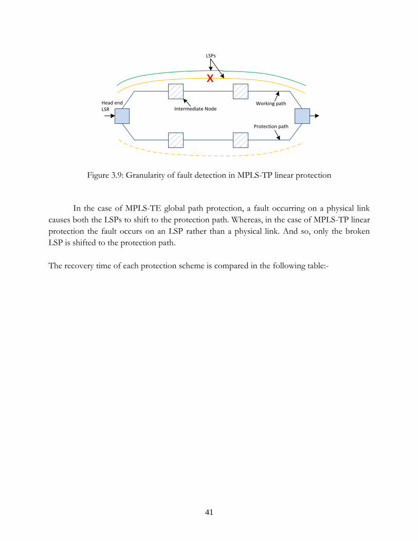
41
Intermediate NodeWorking path
Protection path
LSPs
x
Head end LSR
Figure 3.9: Granularity of fault detection in MPLS-TP linear protection
In the case of MPLS-TE global path protection, a fault occurring on a physical link
causes both the LSPs to shift to the protection path. Whereas, in the case of MPLS-TP linear
protection the fault occurs on an LSP rather than a physical link. And so, only the broken
LSP is shifted to the protection path.
The recovery time of each protection scheme is compared in the following table:-
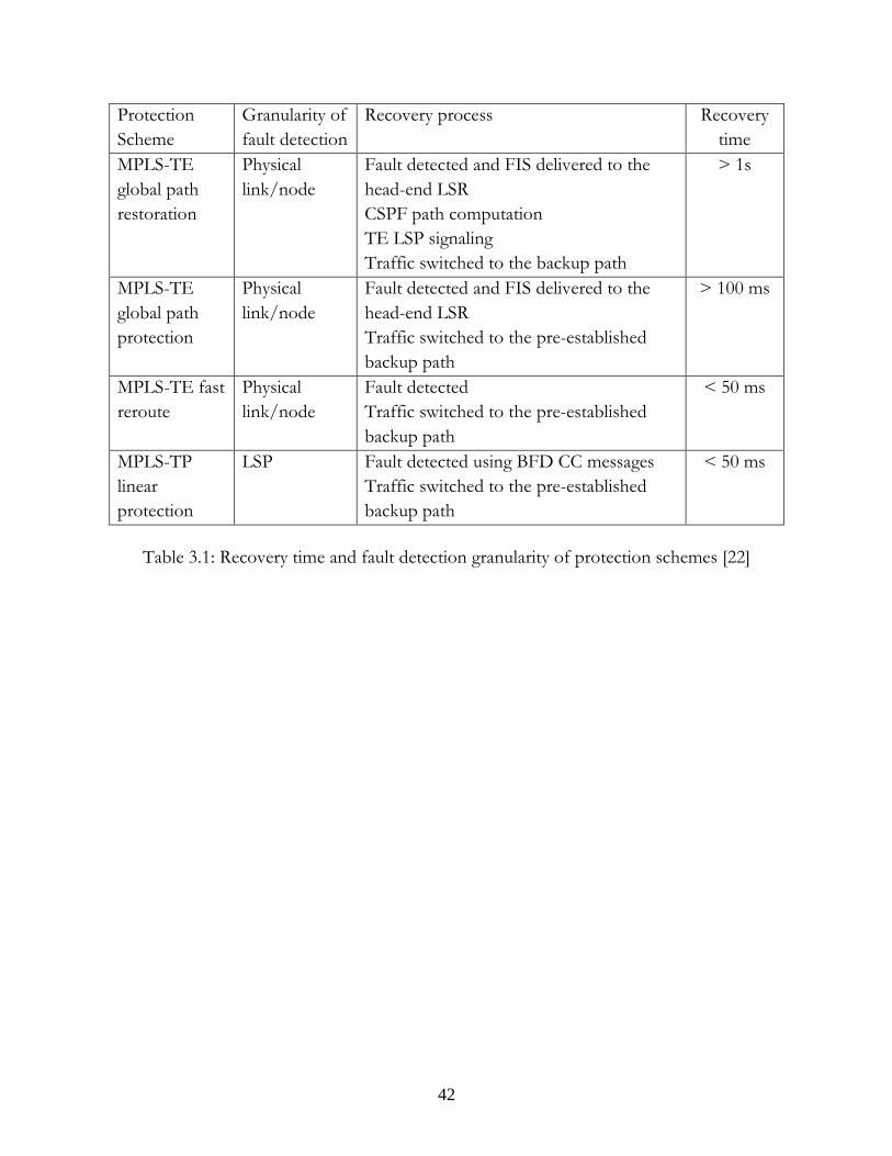
42
Protection
Scheme
Granularity of
fault detection
Recovery process Recovery
time
MPLS-TE
global path
restoration
Physical
link/node
Fault detected and FIS delivered to the
head-end LSR
CSPF path computation
TE LSP signaling
Traffic switched to the backup path
> 1s
MPLS-TE
global path
protection
Physical
link/node
Fault detected and FIS delivered to the
head-end LSR
Traffic switched to the pre-established
backup path
> 100 ms
MPLS-TE fast
reroute
Physical
link/node
Fault detected
Traffic switched to the pre-established
backup path
< 50 ms
MPLS-TP
linear
protection
LSP Fault detected using BFD CC messages
Traffic switched to the pre-established
backup path
< 50 ms
Table 3.1: Recovery time and fault detection granularity of protection schemes [22]

43
Chapter 4
Implementation
4.1. Simulating the PT Radio Condition Signaling Mechanism
For easy prototyping, the Radio Condition Control mechanism of a PT was simulated using
C code. The driver written for Ericsson’s proprietary interface that facilitates communication
between Ericsson’s MiniLink PT device and a network forwarding device is installed on both
the devices. At the PT, some additional code is installed which allows generating control
packets indicating different radio conditions after different time intervals. The rate values and
time intervals can be hardcoded into the C code as desired. Hence, allowing different test
scenarios to be simulated and the behavior of the entire system analyzed. This is intended to
simulate the real behavior of a PT which is supposed to generate radio condition control
messages periodically and whenever there is a change in the modulation scheme on the
microwave link.
For the code to simulate PT’s radio condition signaling mechanism, kernel timers and
workqueues were used. Linux offers the facility that allows the driver to put a process into
sleep state for a defined amount of time. When the timer expires, a predefined function is
called that performs a specific task and can reset the timer so that the task is performed again
later.
Time is referenced in the kernel in Jiffies. This is an unsigned long global kernel
variable used by the kernel scheduler. It is initialized to zero when the system boots up and is
incremented at every clock tick. The clock tick frequency is a configuration option defined in
the config file in the /boot/ directory. The parameter name in this file which defines the tick

44
frequency is CONFIG_HZ. The default value of CONFIG_HZ on a Linux server is 250
which means that there would be 250 clock ticks every second.
Workequeues in Linux allow tasks to be queued for processing at a later time. The
queued jobs are executed by dedicated kernel threads. Since work is done in process context,
the queued jobs can be scheduled for execution later or put into sleep state. Workqueues are
used in many places in the kernel code.
The struct in the Linux kernel which holds all the queued jobs is named
workqueue_struct. Jobs that may need deferred processing are defined using the kernel struct
delayed_work. The macro used to associate a job to its action-function is of the form:-
DECLARE_DELAYED_WORK (struct delayed_work work, work_func_t func)
where work_func_t is a function pointer to the action function. The action function is
responsible for constructing the radio condition control message and transmitting it from the
PT to the network forwarding device. Consequently the transmission rate is limited at the
forwarding device.
The prototype of the function that is used to queue a job in workqueue_struct is:-
int queue_delayed_work (struct workqueue_struct *queue, struct
delayed_work *work, unsigned long delay)
where the delay is specified in jiffies.
4.2. Traffic Rate Control & Buffer Monitoring
On receiving radio condition control frames, the SP modifies its data transmit rate according to the rate value parsed from the frames. This requires modifying the HTB class in the qdisc architecture implemented in the kernel as shown in figure 4.1. The steps to modify the rate at which an htb qdisc dequeues packets for transmission are as follows:-
1. Accessing the root qdisc
struct Qdisc *rootQdisc = netdevice_name->_tx->qdisc;

45
2. Accessing the htb class
#define HTB_CLASSID 65537
unsigned long clptr = rootQdisc->ops->cl_ops->get(rootQdisc,
HTB_CLASSID)
struct htb_class *htbClass = (struct htb_class *)clptr;
3. Modifying the rate
htbClass->rate->rate.rate = rateBps;
This is not enough to actually modify the transmission rate. Once the rate value is set in step 5, the function tc_calc_rtable() implemented in the tc utlity is used to change the rate. The function definition can be found in the file /tc/tc_core.c. In order to switch traffic from the working path to the protection path, the transmit
buffer of the EPI is monitored. To do this, the following steps are carried out:-
1. Accessing the PRIO qdisc
struct Qdisc *prioQdisc = htbClass->un.leaf.q;
2. Accessing the leaf FIFO qdiscs
#define PRIO1_CLASSID 1114113
#define PRIO2_CLASSID 1114114
#define PRIO3_CLASSID 1114115
unsigned long band1id = prioQdisc->ops->cl_ops->get(prioQdisc,
PRIO1_CLASSID);
unsigned long band2id = prioQdisc->ops->cl_ops->get(prioQdisc,
PRIO2_CLASSID);
unsigned long band3id = prioQdisc->ops->cl_ops->get(prioQdisc,
PRIO3_CLASSID);
prio1Qdisc = prioQdisc->ops->cl_ops->leaf(prioQdisc, band1id);
prio2Qdisc = prioQdisc->ops->cl_ops->leaf(prioQdisc, band2id);
prio3Qdisc = prioQdisc->ops->cl_ops->leaf(prioQdisc, band3id);
3. Retrieving the queue length
unsigned int qLen = skb_queue_len (&(prio3Qdisc->q));
Note that the qdisc attached to the third band is monitored because that’s where the traffic packets will be queued.

46
4.3. Qdisc Architecture
Linux kernel uses Queuing Disciplines (Qdiscs) to manage network device queues. The qdisc
architecture employed and the set of rules associated with it determine how packets should
be buffered and scheduled for transmission via an egress network interface. The qdisc
architecture used, as part of the implementation, serves a two-fold purpose:-
1. Providing the ability to rate limit traffic at the SP to proactively prevent congestion on
the microwave link.
2. Prioritizing BFD CC frames over traffic frames along the established LSPs.
As already discussed, radio condition control messages generated by the PT would be
parsed at the SP to deduce the bandwidth available at the microwave link. The qdisc
architecture provides the ability to rate limit traffic at the egress interface.
The qdisc architecture also offers QoS support so that BFD CC messages are strictly
prioritized over traffic packets at every egress interface of the nodes that an LSP traverses.
This is very important since the continuity of BFD CC messages should only be influenced
by a deliberate decision to switch traffic and not due to congestion caused by very high
traffic influx or rate limiting traffic at the SP.
The following figure illustrates the Qdisc architecture used at all the egress interfaces
traversed by the established LSPs:-

47
1:HTB Root Qdisc
HTB Class
PRIO Qdisc
PRIO Classes
1:1
11:
11:1 11:2 11:3
Rate Control
Leaf FIFO Qdisc Leaf FIFO Qdisc
(BFD CC frames queued here)
Leaf FIFO Qdisc
(Traffic frames queued here)
Figure 4.1: Qdisc architecture
The root qdisc is an HTB qdisc with a child HTB class. The HTB class allows
controlling the rate at which packets are dequeued and transmitted. This is followed by a
PRIO qdisc which provides QoS support so that BFD CC frames are prioritized over traffic
frames. It is worth mentioning that the PRIO qdisc also helps achieve the default QoS
behavior of a Linux interface because every Linux interface has a pfifo_fast qdisc by default.
A PRIO qdisc is exactly the same as a pfifo_fast qdisc if not modified.
By default, MPLS frames are queued in the second band i.e. 11:2. To prioritize BFD
CC frames over traffic frames, traffic frames are made to queue up in the third band using a
filter. The filter is applied on the PRIO qdisc. Another approach to achieve the same
behavior could be to queue the BFD CC packets in the first band.
Qdiscs, classes and filters are configured in Linux using the tc utility. The commands
that were used to configure the stated qdisc architecture are mentioned as follows:-

48
# tc qdisc add dev epi0 root handle 1: htb default 1
# tc class add dev epi0 parent 1: classid 1:1 htb rate 792Mbit ceil
792Mbit
# tc qdisc add dev epi0 parent 1:1 handle 11: prio
# tc filter add dev epi0 parent 11: protocol all prio 10 u32
classid 11:3 match u32 0x00000000 0x00000e00 at 0
4.4. Traffic Switching Trigger
The transmission of packets from the SP to the PT will be rate limited if the weather
conditions worsen and the microwave link adopts a modulation scheme that offers a lower
bit rate. This, however, is independent of the amount of traffic that flows into the SP from
its ingress interface. Therefore, a situation can arise where traffic is incident to the SP at a
higher rate compared to the traffic that leaves the SP. As a result, the buffer at the egress
interface of the SP will start filling up.
In a situation where the microwave link is not capable of supporting all the traffic, the
SP should make a decision that it needs to switch part of the traffic to an alternate path. This
decision is very critical and must be made within tens of milliseconds since traffic might be
flowing at gigabit rates. Even the slightest delay can cause a lot of traffic to be lost.
eth1 epi0
SP
Driver1 code
PT
epi0
Driver1 code
3. Buffer build up
4. Ticks
6. Terminate an LSP
5. Checks buffer build up
1. Higher incoming traffic rate 2. Lower outgoing traffic rate
– Driver for the Ericsson proprietary interface – Ericsson proprietary interface
1epi0
Figure 4.2: Traffic switching trigger

49
The approach adopted, as part of the implementation to trigger traffic switching,
relies on a mechanism that generates very rapid periodic ticks. The ticks are generated at
intervals of 3-4 milliseconds. On every tick, the SP checks the state of the buffer at the egress
interface. If the buffer fill-level increases for a defined number of ticks consecutively, the SP
concludes that some traffic needs to be switched to the alternate path. It therefore,
terminates an LSP by dropping the CC packets of its BFD session. Since the configured
LSPs are bidirectional, each LSP corresponds to two BFD sessions. Any one of the two BFD
sessions can be terminated to trigger protection switching.
The number of consecutive ticks, for which the SP waits for the buffer to build up
before it triggers protection switching, must only be big enough so that a congestion
condition is correctly diagnosed. It should ideally be as less as possible so that the overall
process of load balancing is rapid.
The total time it takes from the instance a congestion situation arises to the point
where the end nodes have switched traffic to an alternate path is a sum of two parameters:-
1. Time it takes for the SP to realize that a congestion condition has occurred.
2. Duration of MPLS-TP linear protection switching.
Radio condition control messages are triggered from the PT periodically. They are
also generated whenever there is a change in the modulation scheme on which the
microwave link operates. If the modulation scheme jumps to a higher level e.g. if the weather
conditions get better, the microwave link is able to support a higher data rate. At this time
the SP should shift back some traffic from the secondary path to the primary path. This was
achieved in the code by resuming all terminated BFD sessions whenever a radio condition
control message, with a higher rate value than that at which the SP is already transmitting, is
received. Consequently, the end nodes will synchronize their states using PSC messages and
come to know that the working LSPs are functional again. Once the wait-to-restore time
expires, the end nodes will switch the traffic back to the primary LSPs.
4.5. Timing Parameters
This section discusses in more detail the different timing parameters involved in the load balancing process. The total time involved in the load balancing process is represented by the following equation:-
Timelb = Timediag + Timeswitch

50
Where:-
Timelb represents the total time taken by the load balancing process.
Timediag represents the time taken to diagnose a congestion condition.
Timeswitch represents the time taken by MPLS-TP linear protection switching. It is important to note that Timelb should be less than 50 ms in order to achieve the
goal of rapid protection switching. Therefore, Timediag and Timeswitch must be calibrated to achieve the set goal without affecting system validity and performance.
As mentioned in Section 4.3, Timediag depends on two values. The following equation
shows how Timediag relates to those two values:-
Timediag = Timetick × Tickconsec
Where:-
Timetick represents the tick interval.
Tickconsec represents the number of consecutive ticks it takes for the buffer to build up before traffic is switched to the secondary path. Timetick should neither be too low, as that will burden the processor, nor should it be
too high since that will increase the time taken to detect a congestion condition. Having a high value set for Timetick also constraints the ability to instantaneously respond on frequently fluctuating microwave link conditions. In the thesis implementation this value was set to 3.33 ms.
The value of Tickconsec is again a trade-off between reliability of congestion diagnosis and the time taken to detect the congestion condition. The higher it is, the more reliable is the diagnosis of a congestion condition and the longer it takes to detect the congestion condition and vice versa. It is important to realize here that node processors are usually not the bottleneck in the process of data flow along a communication path. It’s rather the bandwidth offered at the physical layer that is the bottleneck. Therefore, it is safe to assume that packets can be forwarded as rapidly as they are received by the SP if the transmission rate is not limited. The transmit buffer of the SP will only start to fill up once the transmit rate is limited such that it is lower than the rate at which traffic is received. In the thesis implementation the value set for Tickconsec is 6 which is big enough to correctly diagnose a congestion condition. Hence, Timediag is approximately 20 ms.

51
Timeswitch is also comprised of two values. The following equation shows how Timeswitch relates to those two values:-
Timeswitch = Timedetect + Timepsc
Where:-
Timedetect represents the time taken by the receiving end node of the discontinued BFD session to detect that a fault has occurred.
Timepsc represents the PSC convergence time i.e. the time taken by both the end nodes to coordinate their PSC states and start transmitting on the secondary path. As mentioned in Section 2.4.1.1, Timedetect is a product of two values i.e. remote
transmit interval and detect multiplier. This is shown by the following equation:-
Timedetect = Remote TX interval × Detect Multiplier
The minimum values of the transmit interval and detect multiplier that the Ericsson
SP210 device allows for are 3.33 ms and 3 respectively. Same values were used in the implementation for this thesis. That gives a Timedetect of approximately 10 ms.
It could be argued that having very aggressive values set for the transmit interval and
the detect multiplier can cause undesired discontinuity in a BFD session as the intermediate nodes start getting burdened by the overwhelming flow of traffic and node processors are not able to keep up with the strict requirements. But as already discussed in Section 4.2, BFD packets are prioritized over other packets no matter what. So even if the intermediate nodes are burdened with a very high in flux of traffic, they will always let the BFD sessions run smoothly.
It is worth noticing that the even with the least value for the transmit interval a very
negligible amount of bandwidth is consumed. The maximum length of a BFD CC packet on wire is on the order of 100 bytes. A BFD session with a transmit interval of 3.33 ms will generate about 300 packets per second. This results in a bandwidth consumption of 30000 bytes/s or 234 kbps which is negligible compared to the humungous bandwidth offered by links in a service provider’s transport network [20].
Timepsc depends on how fast the end nodes are able to coordinate via the PSC
protocol which in turn depends on the distance between the end nodes or the latency on the path between them. The latency between the end nodes is a function of propagation delay and queuing and processing delays at the intermediate nodes. In the case of the core or transport network of a service provider, though the end nodes must be distant enough, the latency between them is supposed to be very less. And therefore, Timepsc will be much smaller compared to Timediag and Timedetect.

52
The Timelb achieved through the implementation for thesis is therefore:-
Timelb = Timediag + Timeswitch
Timelb = Timediag + Timedetect + Timepsc
Timelb = 20 ms +10 ms + Timepsc
Timelb ≃ 30 ms
So in effect, the goal of Timelb < 50 ms is achieved.
4.6. Lab Setup
The lab setup that was used to demonstrate the thesis idea and generate results is illustrated
in the following figure:-

53
Minilink SP210 Minilink SP210
LSP1 Protection LSP2 Protection
eth1 epi0
SP’
EPI TX Buffer
Driver1 code
epi0 eth1
PT’
Driver1 code
Traffic Generator
1a
2a
LSP1
LSP2
LSP1
LSP2
LSP1
LSP2
Linux servers
1a
2a
3a3a
Radio condition control frames
TX
RX1
Primary path
Backup path
LSP1 traffic rate = 50 Mbps
LSP2 traffic rate = 30 Mbps
4 3
2
– Driver for the Ericsson proprietary interface – Ericsson proprietary interface
1epi0
Figure 4.3: Lab setup

54
The figure above illustrates the lab setup employed in the thesis. The hardware
includes two Ericsson MiniLink SP210 switches, two Linux servers, a traffic generator and
various interconnections between the devices. Ericsson’s MiniLink SP210 switch offers the
MPLS-TP linear protection feature which is the crux of the load balancing solution that is
proposed in this thesis. One Linux server is realized as an SP (labeled SP´), while another
Linux server is realized as a PT (labeled PT´). Both these devices have the driver installed for
Ericsson’s proprietary interface that connects them together. A primary path initiates from
the 1a interface of the first MiniLink SP210 to the 1a interface of the other MiniLink SP210.
This path passes through SP´ and PT´. A backup path is also provided via a direct
connection between the 2a interfaces of both the MiniLink SP210s. Two primary LSPs are
established along the primary path and two corresponding backup LSPs are established along
the backup path. SP´ and PT´ employ the ZebOS routing stack to provide the MPLS label
switching functionality.
A traffic generator is used to generate traffic for both the LSPs independently. This is
achieved by encapsulating packets originating from the traffic generator with 802.1Q VLAN
headers. Different VLAN tags are used for traffic belonging to LSP1 and LSP2. At the
MiniLink SP210s two pseudowires are configured, each passing through either LSP1 or
LSP2. A mapping is created between traffic VLAN tags and the pseudowires in VFI of the
MiniLink SP210s. Using this mapping, the MiniLink SP210 receiving traffic from the traffic
generator knows which LSP a packet should be sent on. For the sake of demonstration,
traffic is generated at different rates for LSP1 and LSP2. For LSP1 traffic is generated at 50
Mbps whereas for LSP2 traffic is generated at 30 Mbps.
PT´ generates radio condition control messages as the test scenario hardcoded in its
driver code dictates. SP´ receives these radio condition control messages, parses the received
rate value and adjusts its transmission rate towards PT´. At SP´, the transmission buffer of
the EPI is monitored to decide when traffic must be switched to the backup path.
The traffic generator generates four graphs from its four connections as illustrated in
the figure. These graphs can be analyzed to see how traffic switches between the primary and
backup path.

55
Chapter 5
Results & Discussion
This chapter describes how the implemented system was used to generate results which
justify the validity of the load balancing concept. The results advocate the correctness of the
system’s functionality, system performance and robustness. This chapter also includes a
discussion section which specifically discusses certain aspects in the graphical results
presented and system stability under varying network conditions.
5.1. Results
To demonstrate the results a test scenario was hardcoded in PT´. The test scenario was
designed to demonstrate the load balancing concept and to show how traffic is switched to
and from the working and protection paths when different radio condition control messages
are generated by PT´.
In the test scenario coded at PT´, three different radio condition control messages are
generated at different instances. A radio condition control message can contain a rate value
of 140 Mbps, 70 Mbps or 30 Mbps. As mentioned earlier, the traffic rate of LSP1 is 50 Mbps
while the traffic rate of LSP2 is 30 Mbps. The sequence of radio condition control messages
and their timings were hardcoded in the test scenario such that four different behavioral
patterns could be demonstrated. The four different behavioral patterns are mentioned as
follows:-

56
1. One LSP is switched to the protection path upon receipt of a radio condition control
message.
2. Both the LSPs are switched to the protection path together upon receipt of a radio
condition control message.
3. Both the LSPs are switched to the protection path, one at a time, as two successive
radio condition control messages are received.
4. One or both the LSPs are switched from the protection path to the working path
after a radio condition control message is received and the Wait-to-Restore time
elapses.
The traffic generator generates four different graphs. The following table shows what
each graph signifies, line color of the graph, and the corresponding interface (indicated by an
interface number figure 4.3) on the traffic generator for each graph:-
Interface Line color Graph
1 Total traffic TX rate
2 Total traffic RX rate
3 Rate of traffic passing on the primary path
4 Rate of traffic passing on the backup path
Table 5.1: Traffic generator graphs
The following figure illustrates a timeline which shows the exact sequence and timings
of the different radio condition control messages generated from PT´ through the hardcoded
test scenario. It also points out the radio condition control messages responsible for
demonstrating the four different behavioral patterns listed above. The figures that follow the
next figure show the graphs that were generated by the traffic generator when the test
scenario was run.

57
WTR (5 mins)LSP1 à PLSP2 à P
LSP1 à WLSP2 à W
LSP1 à WLSP2 à P
WTR (5 mins)LSP1 à WLSP2 à P
LSP1 à WLSP2 à W
LSP1 à PLSP2 à P
WTR (5 mins)LSP1 à PLSP2 à P
LSP1 à WLSP2 à W
LSP1 à WLSP2 à P
LSP1 à PLSP2 à P
00:00 22:00
01:00 02:00 03:00 04:00 05:00 06:00 07:00 08:00 09:00 10:00 11:00 12:00 13:00 14:00 15:00 16:00 17:00 18:00 19:00 20:00 21:00
Flow control messageRate = 140 Mbps
Flow control messageRate = 70 Mbps
Flow control messageRate = 140 Mbps
Flow control messageRate = 30 Mbps
Flow control messageRate = 140 Mbps
Flow control messageRate = 70 Mbps
Flow control messageRate = 30 Mbps
Time (mins)
LEGEND
WTR – Wait to RestoreW – Working pathP – Protection path
Behavioral Pattern 1 Behavioral Pattern 4 Behavioral Pattern 2 Behavioral Pattern 3
Data Rates
LSP1 – 50 MbpsLSP2 – 30 MbpsTotal – 80 Mbps
Behavioral Pattern 1 à LSP2 switches to the protection path with SP´ TX rate set to 70 Mbps.
Behavioral Pattern 2 à Both LSPs switch to the protection path with SP´ TX rate set to 30 Mbps.
Behavioral Pattern 3 à First LSP2 switches to the protection path when SP´ TX rate is set to 70 Mbps, then LSP1 also switches to the protection path when SP´ TX rate is set to 30 Mbps.
Behavioral Pattern 4 à Any LSP on the protection path switches to the working path after SP´ TX rate is set to 140 Mbps and WTR elapses.
Figure 5.1: Timeline for the test scenario simulated at PT´

58
Figure 5.2: Results (TX rate graphs)

59
(b) (c)
(a)
Figure 5.3: Results (RX rate graphs – First Half)

60
(b) (c) (d) (e) (f)
(a)
Figure 5.4: Results (RX rate graphs – Second Half)

61
The traffic generator generates a TX graph, which shows the rate at which data is
transmitted from its four interfaces, and an RX graph, which shows the rate at which data is
received on its four interfaces. Data generated by the traffic generator is sent out of interface
1. So interface 1 only transmits data whereas interface 2, 3 and 4 only receive data. This is
evident from the TX graph, in figure 5.2, which shows data being sent out of interface 1 at
80 Mbps i.e. sum of data being sent on LSP1 and LSP2. Data is constantly transmitted at a
fixed rate from the traffic generator hence the TX graph is constant. This, however, is not
the case with the RX graphs. The RX graphs show frequent variations which are the result of
traffic being shifted to and from the working and protection paths.
The RX graph, in figure 5.3 and 5.4, remains constant for two ports. For interface 1,
the graph stays constant on zero since data is only transmitted from interface 1 and not
received. For interface 2, the graph mostly stays constant on 80 Mbps. This is as desired
because the system should be able to successfully transport any data generated by the traffic
generator at all times, regardless the traffic switching events between the primary and the
secondary path.
More important variations occur in graphs generated at interface 3 and 4 which
represent the data received on the primary and secondary path respectively. Before the driver
for the EPI is installed on SP´ and PT´, all data flows on the backup path. As soon as the
driver code is installed on SP´ and PT´, the working path is established. A WTR time of five
minutes was configured on the Ericsson MiniLink SP210 devices. Therefore, after the
working path is established data of both the LSPs keeps flowing through the backup path for
the next five minutes. This is evident from figure 5.3 where, for the first 300 seconds, the
graph representing the data flowing on the secondary path is constant on a little more than
110 Mbps while the graph representing the data flowing on the primary path is constant on
zero. It is important to note here that data flows on the backup path at 110 Mbps although
the traffic generator generates the data at a total rate of 80 Mbps. This is because of the
MPLS header encapsulation plus the header appended by the EPI driver.
After the WTR time elapses, both the LSPs are switched to the working path. This is
illustrated in figure 5.3 (b). At t = 6 mins, a radio condition control message with rate value
70 Mbps is generated. Now only LSP1 can be supported on the primary path and LSP2
should be shifted to the backup path. This is evident from figure 5.3 (c) where both the
working and protection path start transporting data. Note that this corresponds to behavioral
pattern 1 as described in figure 5.1.

62
At t = 7 mins, a radio condition control message with rate value 140 Mbps is
generated. Now both the LSPs can be supported on the working path. At this point the
WTR timer starts again. At t = 12 mins, LSP2 switches back to the primary path. This is
illustrated in figure 5.4 (b). Note that this corresponds to behavioral pattern 4 as described in
figure 5.1.
At t = 13 mins a radio condition control message, with rate value 30 Mbps, is
generated. With a transmission rate of 30 Mbps, LSP2 can be supported on the primary path.
But the implementation terminates the LSPs in a predetermined fashion where LSP2 is
terminated first and LSP1 follows. So at this point, both the LSPs are switched to the
protection path which is evident from figure 5.4 (c). Note that this corresponds to behavioral
pattern 2 as described in figure 5.1.
At t = 20 mins, a radio condition control message, with rate value 70 Mbps, is
generated. As a result LSP2 switches to the protection path which is illustrated in figure 5.4
(e). At t = 21 mins, another radio condition control message with rate value 30 Mbps is
generated. As a result, LSP1 also switches to the protection path. This is illustrated in figure
5.4 (f). Note that this corresponds to behavioral pattern 3 as described in figure 5.1.
5.2. Discussion
From the graphs generated by the traffic generator, it can be seen that data is received at
interface 2 of the traffic generator at 80 Mbps. This is as expected if there were to be no data
loss, since the total data is sent at 80 Mbps at all times. However, the data rates indicated by
graphs of interface 3 and 4 sum up to approximately 110 Mbps. This increase in data is due
to MPLS header encapsulation plus the header appended by the EPI driver.
Figure 5.4 (c) clearly illustrates a dip in data received at interface 2. This indicates data
loss which is caused during traffic switching from primary to secondary path. Packet loss
occurs because the transmit buffer of SP´ will have some packets at the time of switching.
Once switching completes, the receiving node will discard any packets sent from the transmit
buffer of SP´ on the working path. The motive behind achieving rapid traffic switching i.e. in
the order of tens of milliseconds is to minimize this data loss as much as possible.
The load balancing idea presented in this thesis involves traffic switching to and from
the primary and secondary path depending on the bandwidth conditions of the affected
microwave link. This means that traffic should be shifted back from the secondary path to

63
the primary path as soon as the bandwidth conditions on the microwave link improve.
However, this behavior has certain implications. Flickering radio link conditions can cause
the offered bandwidth to change several times during a couple of seconds or in other words
can cause system oscillation. Switching traffic so rapidly in the system has several downsides
that include data loss, processing load and overall system instability. This should be handled
by avoiding traffic switching if the microwave link flickers. Traffic should only be switched
to alternate paths if it is triggered by more permanent changes in weather.
Ericsson MiniLink SP210 nodes offer a minimum WTR time of 5 minutes. Therefore
as part of system testing, analyzing the system behavior with very frequently generated radio
condition control messages was not possible. Though this thesis functionally verifies the idea
of load balancing traffic using MPLS-TP linear protection, further optimizations are
necessary to achieve full system stability.

64
Chapter 6
Conclusion
Though MPLS-TP linear protection was invented as part of the inherent protection
mechanisms of MPLS-TP, it can very elegantly be used to load balance traffic in packet
switched networks. Legacy transport network technologies like SDH/SONET offer
protection mechanisms which allow traffic switching to occur in as less as few tens of
milliseconds. However, the granularity of fault detection is limited to a physical link or node.
MPLS-TP, on the other hand, allows in-band OAM messages to be sent through the
configured LSPs. OAM sessions of an LSP are independent of the OAM sessions of other
LSPs. This enables monitoring each LSP independently, hence allowing fault detection at the
granularity of an LSP.
The ability to detect faults at the granularity of a virtual path rather than a physical
path leads to another intelligent application i.e. load balancing traffic. With a set of primary
and secondary LSPs established on link/node diverse physical paths, a deliberate attempt to
create a fault in a subset of the working LSPs can enable traffic to be partially shifted to the
secondary physical path. With a bigger picture of a real world carrier network, this
application particularly suits to communication paths which comprise microwave links.
Microwave links suffer from varying weather conditions and hence varying bandwidth
capacity which can lead to traffic congestion.
Carrier networks carry a huge amount of data. Any protection or load balancing
mechanisms employed must be very rapid so as to minimize data loss. MPLS-TP linear
protection relies on BFD CC messages to monitor the liveliness of an LSP. Unlike the
“Hello” mechanisms provided by routing protocols, the BFD protocol offers a failure
detection time in the order of tens of milliseconds.

65
6.1. Summary of Work
This Master’s thesis work shows how MPLS-TP linear protection can be used to balance
traffic load in a network comprising microwave nodes. As part of the tasks accomplished in
this Master’s thesis, a driver for an Ericsson proprietary digital network interface was
developed in Linux kernel space. This interface facilitates communication between Ericsson’s
MiniLink PT microwave node and any network forwarding device like Ericsson’s MiniLink
SP node.
A radio condition signaling mechanism was implemented in the driver. This
mechanism is used by the PT to inform the SP of the microwave link state. The radio
condition signaling mechanism is imperative in accomplishing the load balancing goal. Radio
condition control packet generation was simulated at the PT. At the SP, a Qdisc architecture
was deployed which enabled modifying the transmission rate of the SP to align with the rate
value received in the radio condition control messages. The Qdisc architecture also provides
QoS support to strictly prioritize BFD CC messages over traffic packets.
A load balancing module was also implemented at the SP. The load balancing module
monitors the transmit buffer of the EPI at all times and triggers traffic switching if the buffer
starts building up due to a difference in the incoming and outgoing traffic rate.
To conclude the work, a demonstration was carried out with two MiniLink SP210s,
two Linux servers realized as SP and PT and a traffic generator. Two pairs of working and
protection LSPs were established. A test scenario was hardcoded in the PT to demonstrate
different behavioral patterns of traffic flow. The traffic generator was used to generate traffic
and produce graphs indicating the traffic rate on the primary and secondary paths.
6.2. Future Work
The idea of using MPLS-TP linear protection as a means to load balance traffic in microwave
networks is ingenious. The implementation carried out in this thesis provides the foundation
for a realistic solution. But to realize the load balancing concept in a real world network, a
number of other factors need to be considered such as:-
Bandwidth conditions on alternate communication paths: The thesis presents the idea
of switching traffic to alternate paths in a network if there is service degradation
somewhere along the primary path. But the alternate paths may be the preferred paths

66
for certain traffic streams. Switching traffic to these paths without considering the
available bandwidth conditions on them could result in service degradation. There are
chances that the alternate paths may be experiencing worse bandwidth conditions
compared to the primary path. In that case, it is preferable not to switch any traffic.
Hence, there should be a mechanism through which all nodes along a path and its
backup path share their transmit buffer states. Before switching traffic, a node can
then compare the conditions on the primary and secondary path to determine if
switching traffic is ideal.
Switching traffic discriminately: Traffic exhibits different characteristics e.g. delay
tolerant/intolerant, loss tolerant/intolerant etc. When switching traffic, it is important
to analyze traffic nature and criticality. Interruptions in high priority traffic should be
avoided. Traffic streams can be mapped to distinct LSPs based on their
characteristics. On service degradation, LSPs carrying less critical traffic can be
switched to the secondary path first.
Section 3.5 presents the technique employed to determine when traffic should be
switched to a secondary path. It is worth emphasizing that the technique used is very critical.
It must not only be rapid, but it must also be able to correctly identify a congestion
condition. The technique used in this thesis involves checking the transmit buffer queue
length of the EPI at the SP iteratively. It the queue length increases consecutively for a
certain number of iterations, an LSP on the working path is terminated. Consequently, the
LSP is switched to the secondary path. LSPs are terminated in a predetermined order i.e.
LSP2 is terminated before LSP1.
This technique should be evaluated against other possible options so that the process
of traffic switching can be optimized in terms of its speed and correctness. A couple of other
options that can be proposed are as follows:-
The instantaneous traffic rate of individual LSPs can be determined by measuring the
amount of bytes received on each LSP in a short time interval. Hence, the total
incoming traffic rate can be determined and compared with the transmission rate set
to decide if traffic should be switched to the alternate path. This technique also offers
the flexibility of switching the LSP with the lowest traffic rate so that only enough
traffic is moved to the alternate path as required.
Another way could be to set a threshold for buffer build-up based on the transmit
rate set at the SP and terminate an LSP if the threshold is exceeded.

67
Bibliography [1] Wehrle, Klaus. "Managing Network Packets in the Kernel." The Linux Networking
Architecture: Design and Implementation of Network Protocols in the Linux Kernel. Upper
Saddle River, NJ: Pearson Prentice Hall, 2004. 55-66. Print.
[2] Chimata, Ashwin Kumar. "Path of a Packet in the Linux Kernel Stack." N.p., 11 July
2005. Web. 20 Oct. 2012.
<http://hsnlab.tmit.bme.hu/twiki/pub/Targyak/Mar11Cikkek/Network_stack.pdf>
[3] "Linux Networking Kernel." N.p., 12 Feb. 2003. Web.
<http://www.ecsl.cs.sunysb.edu/elibrary/linux/network/LinuxKernel.pdf>
[4] Kelly, Richard, and Joseph Gasparakis. (2010). Common Functionality in the 2.6
Linux Network Stack. [White paper]. Retrieved from
<http://download.intel.com/design/intarch/PAPERS/323704.pdf>.
[5] Vandecappelle, Arnout. "Kernel Flow." The Linux Foundation. N.p., 19 Nov. 2009.
Web. 20 Oct. 2012.
<http://www.linuxfoundation.org/collaborate/workgroups/networking/kernelflow
>.
[6] Wehrle, Klaus. "Using Traffic Control to Support Quality of Service (QoS)." The
Linux Networking Architecture: Design and Implementation of Network Protocols in the Linux
Kernel. Upper Saddle River, NJ: Pearson Prentice Hall, 2004. 367. Print.
[7] Balliache, Leonardo. "Linux Traffic Control." Differentiated Service on Linux HOWTO.
N.p., Aug. 2003. Web. 19 Oct. 2012. <http://opalsoft.net/qos/DS.htm>.

68
[8] Hubert, Bert. "Simple, Classless Queueing Disciplines." Linux Advanced Routing &
Traffic Control HOWTO. N.p., 22 July 2002. Web. 19 Oct. 2012.
<http://www.tldp.org/HOWTO/Adv-Routing-
HOWTO/lartc.qdisc.classless.html>.
[9] "The pfifo_fast Queuing Discipline." N.p., N.d. Retrieved from http://ace-
host.stuart.id.au/russell/files/tc/doc/sch_pfifo_fast.txt
[10] Brown, Martin A. "Classless Queuing Disciplines (qdiscs)." Traffic Control HOWTO.
N.p., Oct. 2006. Web. 19 Oct. 2012. <https://www.linux.com/learn/docs/ldp/783-
traffic-control-howto>.
[11] tc-tbf(8)-Linux man page. (n.d.). Retrieved from http://linux.die.net/man/8/tc-tbf
[12] Hubert, Bert, Gregory Maxwell, Remco Van Mook, Martijn Van Oosterhout, Paul B.
Schroeder, and Jasper Spaans. "Classful Queueing Disciplines." Linux Advanced Routing
& Traffic Control HOWTO. N.p., July 2002. Web. 20 Oct. 2012.
<http://www.tldp.org/HOWTO/Adv-Routing-HOWTO/lartc.qdisc.classful.html>.
[13] Balliache, Leonardo. "PRIO Queuing Discipline." Differentiated Service on Linux
HOWTO. N.p., Aug. 2003. Web. 20 Oct. 2012. <http://opalsoft.net/qos/DS.htm>.
[14] Brown, Martin A. "Classful Queuing Disciplines (qdiscs)." Traffic Control HOWTO.
N.p., Oct. 2006. Web. 19 Oct. 2012. <https://www.linux.com/learn/docs/ldp/783-
traffic-control-howto>.
[15] Lieven Levrau and Lou Berger, “A Framework for MPLS in Transport Networks,”
RFC 5921, July 2010. [Online]. Available: http://tools.ietf.org/html/rfc5921
[16] Matthew Bocci (ed.), Martin Vigoureux (ed.) and Stewart Bryant (ed.), “MPLS
Generic Associated Channel,” RFC 5586, June 2009. [Online]. Available:
https://tools.ietf.org/html/rfc5586
[17] Cisco System, Inc. (2009). Understanding MPLS-TP and its benefits [White paper].
Retrieved from
http://www.cisco.com/en/US/technologies/tk436/tk428/white_paper_c11-
562013.pdf

69
[18] Stewart Bryant, Eric Osborne and Nurit Sprecher, “MPLS Transport Profile (MPLS-
TP) Linear Protection,” RFC 6378, October 2011. [Online]. Available:
http://tools.ietf.org/html/rfc6378
[19] Annamaria Fulignoli, Sami Boutros, Martin Vigoureux, Siva Sivabalan, David Ward,
Robert Rennison, ” Proactive Connectivity Verification, Continuity Check, and
Remote Defect Indication for the MPLS Transport Profile,” RFC 6428, November
2011. [Online]. Available: http://tools.ietf.org/html/rfc6428
[20] Dave Katz and Dave Ward, “Bidirectional Forwarding Detection (BFD),” RFC 5880,
June 2010. [Online]. Available: http://tools.ietf.org/html/rfc5880
[21] Davie, Bruce S., and Adrian Farrel. "MPLS Traffic Engineering Recovery
Mechanisms." MPLS: Next Steps. San Francisco, CA: Elsevier/Morgan Kaufmann,
2008. 160-205. Print.
[22] Vasseur, JP, MPLS Deployment Forum, March 2002, London. Cisco Systems Inc.
n.p. Lecture.
[23] Recommendation ITU-T G.808.1 (2010), Generic protection switching – Linear trail and
subnetwork protection.
[24] Recommendation ITU-T G.808.1 Amendment 2 (2012), Generic protection switching –
Linear trail and subnetwork protection.