lncs 4170 - a sparse object category model for …vgg/publications/2006/fergus06/fergus06.pdf · j....

A Sparse Object Category Model for EfficientLearning and Complete Recognition

Rob Fergus1, Pietro Perona2, and Andrew Zisserman1

1 Dept. of Engineering ScienceUniversity of OxfordParks Road, Oxford

OX1 3PJ, U.K.{fergus,az}@robots.ox.ac.uk

2 Dept. of Electrical EngineeringCalifornia Institute of Technology

MC 136–93, PasadenaCA 91125, U.S.A.

[email protected]

Abstract. We present a “parts and structure” model for object cate-gory recognition that can be learnt efficiently and in a weakly-supervisedmanner: the model is learnt from example images containing category in-stances, without requiring segmentation from background clutter.

The model is a sparse representation of the object, and consists of astar topology configuration of parts modeling the output of a variety offeature detectors. The optimal choice of feature types (whose repertoireincludes interest points, curves and regions) is made automatically.

In recognition, the model may be applied efficiently in a completemanner, bypassing the need for feature detectors, to give the globallyoptimal match within a query image. The approach is demonstrated ona wide variety of categories, and delivers both successful classificationand localization of the object within the image.

1 Introduction

A variety of models and methods exist for representing, learning and recogniz-ing object categories in images. Many of these are variations on the “Parts andStructure” model introduced by Fischler and Elschlager [10], though the moderninstantiations use scale-invariant image fragments [1,2,3,12,15,20,21]. The con-stellation model [3,8,21] was the first to convincingly demonstrate that modelscould be learnt from weakly-supervised unsegmented training images (i.e. theonly supervision information was that the image contained an instance of theobject category, but not the location of the instance in the image). Various typesof categories could be modeled, including those specified by tight spatial config-urations (such as cars) and those specified by tight appearance exemplars (suchas spotted cats). The model was translation and scale invariant both in learningand in recognition.

J. Ponce et al. (Eds.): Toward Category-Level Object Recognition, LNCS 4170, pp. 443–461, 2006.c© Springer-Verlag Berlin Heidelberg 2006

444 R. Fergus, P. Perona, and A. Zisserman

However, the Constellation model of [8] has some serious short-comings,namely: (i) The joint nature of the shape model results in an exponential explo-sion in computational cost, limiting the number of parts and regions per imagethat can be handled. For N feature detections, and P model parts the complexityfor both learning and recognition is O(NP ); (ii) Since only 20-30 regions per im-age and 6 parts are permitted by this complexity, the model can only learn froman incredibly sparse representation of the image. Good performance is thereforehighly dependent on the consistent firing of the feature detector; (iii) Only onetype of feature detector (a region operator) was used, making the model verysensitive to the nature of the class. If the distinctive features of the categoryhappen, say, to be edge-based then relying on a region-based detector is likelyto give poor results (though this limitation was overcome in later work [9]); (iv)The model has many parameters resulting in over-fitting unless a large numberof training images (typically 200+) are used.

Other models and methods have since been developed which have achievedsuperior performance to the constellation model on at least a subset of the ob-ject categories modeled in [8]. These models range from bag-of-word models(where the words are vector quantized invariant descriptors) with no spatial or-ganization [5,18], through to fragment based models [2,15] with particular spatialconfigurations. The methods utilize a range of machine learning approaches EM,SVMs and Adaboost.

In this paper we propose a heterogeneous star model (HSM) which main-tains the simple training requirements of the constellation model, and also,like the constellation model, gives a localization for the recognized object. Themodel is translation and scale invariant both in learning and in recognition.There are three main areas of innovation: (i) both in learning and recognitionit has a lower complexity than the constellation model. This enables both thenumber of parts and the number of detected features to be increased substan-tially; (ii) it is heterogeneous and is able to make the optimum selection offeature types (here from a pool of three, including curves). This enables it tobetter model objects with significant intra-class variation in appearance, butless variation in outline (for example a guitar), or vice-versa; (iii) The recog-nition stage can use feature detectors or can be complete in the manner ofFelzenswalb and Huttenlocher [6]. In the latter case there is no actual detec-tion stage. Rather the model itself defines the areas of most relevance using amatched filter. This complete search overcomes many false negatives due to fea-ture drop out, and also poor localizations due to small feature displacement andscale errors.

2 Approach

We describe here the structure of the heterogeneous star model, how it is learntfrom training data, and how it is applied to test data for recognition.

A Sparse Object Category Model 445

2.1 Star Model

As in the constellation model of [8], our model has P parts and parametersθ. From each image i, we extract N features with locations Xi; scales Si anddescriptors Di. In learning, the aim is to find the value of θ that maximizes thelog-likelihood over all images:

∑i

log p(Xi,Di,Si|θ) (1)

Since N >> P , we introduce an assignment variable, h, to assign features toparts in the model. The log-likelihood is obtained by marginalizing over h.

∑i

log∑h

p(Xi,Di,Si,h|θ) (2)

In the constellation model, the joint density is factored as:

p(Xi,Di,Si,h|θ) = p(Di|h, θ)︸︷︷︸Appearance

p(Xi|Si,h, θ)︸︷︷︸Rel. Locations

p(Si|h, θ)︸︷︷︸Rel. Scale

p(h|θ)︸︷︷︸Occlusion

(3)

In [8], the appearance model for each part is assumed independent but the rel-ative location of the model parts is represented by a joint Gaussian density.While this provides the most thorough description, it makes the location of allparts dependent on one another. Consequently, the EM-based learning scheme,which entails marginalizing over p(h|Xi,Di,Si, θ), becomes an O(NP ) opera-tion. We propose here a simplified configuration model in which the location of

x1

x3

x4

x6

x5

x2

Fully connected model

x1

x3

x4

x6

x5

x2

Fully connected model

(a)

x1

x3

x4

x6

x5

x2

“Star” model

x1

x3

x4

x6

x5

x2

“Star” model

(b)

Fig. 1. (a) Fully-connected six part shape model. Each node is a model part whilethe edges represent the dependencies between parts. (b) A six part Star model. Theformer has complexity O(NP ) while the latter has complexity O(N2P ) which may befurther improved in recognition by the use of distance-transforms [6] to O(NP ).

the model part is conditioned on the location of a landmark part. Under thismodel the non-landmark parts are independent of one another given the land-mark. In graphical model terms, this is a tree of depth one, with the landmark


part being the root node. We call this the “star” model. A similar model, wherethe reference frame acts as a landmark is used by Lowe [16] and was studied in aprobabilistic framework by Moreels et al. [17]. Figure 1 illustrates the differencesbetween the full and star models. In the star model the joint probability of theconfiguration aspect of the model may be factored as:

p(X|S,h, θ) = p(xL|hL)∏j �=L

p(xj |xL, sL, hj , θj) (4)

where xj is the position of part j and L is the landmark part. We adopt aGaussian model for p(xj |xL, sL, hj , θj) which depends only on the relative posi-tion and scale between each part and the landmark. The reduced dependenciesof this model mean that the marginalization in Eqn. 2 is O(N2P ), in theoryallowing us to cope with a larger N and P in learning and recognition.

In practical terms, we can achieve translation invariance by subtracting thelocation of the landmark part from the non-landmark ones. Scale invarianceis achieved by dividing the location of the non-landmark parts by the locallymeasured scale of the landmark part.

It is useful to examine what has been lost in the star compared to the constel-lation model of [8]. In the star model any of the leaf (i.e. non-landmark) partscan be occluded, but (as discussed below) we impose the condition that the land-mark part must always be present. With small N this can lead to a model withartificially high variance, but as N increases this ceases to be a problem (sincethe landmark is increasingly likely to actually be detected). In the constellationmodel any or several parts can be occluded. This is a powerful feature: not onlydoes it make the model robust to the inadequacies of the feature detector but italso assists the convergence properties of the model by enabling a subset of theparts to be fitted rather than all simultaneously.

The star model does have other benefits though, in that it has less parametersso that the model can be trained on fewer images without over-fitting occurring.

2.2 Heterogeneous Features

By constraining the model to operate in both learning and recognition from thesparse outputs of a feature detector, good performance is highly dependent onthe detector finding parts of the object that are characteristic and distinctiveof the class. The majority of approaches using feature-based methods rely onregion detectors such as Kadir and Brady or multi-scale Harris [11,13] whichfavour interest points or circular regions. However, for certain classes such asbottles or mugs, the outline of the object is more informative than the texturedregions on the interior. Curves have been used to a limited extent in previousmodels for object categories, for example both Fergus et al. [9] and Jurie &Schmid [12] introduce curves as a feature type. However, in both cases the modelwas constrained to being homogeneous, i.e. consisting only of curves. Here themodels can utilize a combination of different features detectors, the optimalselection being made automatically. This makes the scheme far more tolerant tothe type of category to be learnt.


20 40 60 80 100 120 140 160 180 200 220

20

40

60

80

100

120

140

20 40 60 80 100 120 140 160 180 200 220

20

40

60

80

100

120

140

20 40 60 80 100 120 140 160 180 200 220

20

40

60

80

100

120

140

20 40 60 80 100 120 140 160 180 200 220

20

40

60

80

100

120

140

20 40 60 80 100 120 140 160 180 200 220

20

40

60

80

100

120

140

20 40 60 80 100 120 140 160 180 200 220

20

40

60

80

100

120

140

(a) (b) (c)

Fig. 2. Output of three different feature detectors on two airplane images. (a) Curves.(b) Kadir & Brady. (c) Multi-scale Harris.

In our scheme, we have a choice of three feature types: Kadir & Brady; multi-scale Harris and Curves. Figure 2 shows examples of these 3 operators on twosample airplane images. The detectors were chosen since they are somewhat com-plementary in their properties: Kadir & Brady favours circular regions; multi-scale Harris prefers interest points, and curves locate the outline of the object.

To be able to learn different combinations of features we use the same rep-resentation for all types. Inspired by the performance of PCA-SIFT in regionmatching [14], we utilize a gradient-based PCA approach in contrast to theintensity-based PCA approach of [8]. Both the region operators give a locationand scale for each feature. Each feature is cropped from the image (using a squaremask); rescaled to a k×k patch; has its gradient computed and then normalizedto remove intensity differences. Note that we do not perform any orientationnormalization as in [14]. The outcome is a vector of length 2k2, with the first kelements representing the x derivative, and the second k the y derivatives. Thederivatives are computed by symmetric finite difference (cropping to avoid edgeeffects).

The normalized gradient-patch is then projected into a fixed PCA basis1 ofd dimensions. Two additional measurements are made for each gradient-patch:its unnormalized energy and the reconstruction error between the point in thePCA basis and the original gradient-patch. Each region is thus represented by avector of length d + 2.

Curve features are extracted in the same manner as [9]: a Canny edge detectoris run over the image; the edgels are grouped into chains; each chain is then

1 The fixed basis was computed from patches extracted using all Kadir and Bradyregions found on all the training images of Motorbikes; Faces; Airplanes; Cars (Rear);Leopards and Caltech background.


broken at its bitangent points to give a curve. Since the chain may have multiplebitangent points, each chain may result in multiple curves (which may overlapin portions). Curves which are very straight tend to be uninformative and arediscarded.

The curves are then represented in the same way as the regions. Each curve’slocation is taken as its centroid with the scale being its length. The region aroundthe curve is then cropped from the image and processed in the manner describedabove. We use the curve as an feature detector, modeling the textured regionaround the curve, rather than the curve itself. Modeling the actual shape of thecurve, as was done in [9], proved to be uninformative, in part due to the difficultyof extracting the contours consistently enough.

2.3 Learning the Model

Learning a heterogeneous star model (HSM) can be approached in several ways.One method is to learn a fully connected constellation model using EM [8] andthen reduce the learnt spatial model to a star by completely trying out each ofthe parts as a landmark, and picking the one which gives the highest likelihoodon the training data. The limitation of this approach is that the fully connectedmodel can only handle a small number of parts and detections in learning. Thesecond method, which we adopt, is to learn the HSM directly using EM as in[8,21], starting from randomly-chosen initial conditions, enabling the learning ofmany more parts and with more detections/image.

Due to the more flexible nature of the HSM, successful learning depends ona number of factors: To avoid combinatorics inherent in parameter space andto ensure the good convergence properties of the model, an ordering constraintis imposed on the locations of the model parts (e.g. the x-coordinates mustbe increasing). However, to enable the landmark part to select the most stablefeature on the object (recall that we force it to always be present), the land-mark is not subject to this constraint. Additionally, each part is only allowedto pick features of a pre-defined type and the ordering constraint only applieswithin parts of the same type. This avoids over-constraining the shape model.Imposing these constraints prevents exact marginalization in O(N2P ), howeverby using efficient search methods, an approximation can be computed using allhypotheses within a threshold δ of the best hypothesis that obeys the constraint(δ = e−10 in our experiments). In Figure 3, the mean time per iteration perframe in learning is shown as N and P are varied. In Figure 3(a) P is fixed at 6and N varied from 20 up to 200 while recording the mean time per image overall EM iterations in learning. The curve has a quadratic shape with the time perimage still respectable even for N = 200. It should be noted that a full modelcannot be learnt with N > 25 due to memory requirements. In Figure 3(b) N isfixed at 20 and P varied from 2 to 13 with the mean time per image plotted on alog-scale y-axis. The curve for the full model is a straight line as expected fromthe O(NP ) complexity, stopping at P = 7 owing to the memory overhead. The


20 40 60 80 100 120 140 160 180 2000

0.05

0.1

0.15

0.2

0.25

0.3

0.35

Me

an

tim

e /

ite

ratio

n /

im

ag

e (

se

cs)

Number of Detections

(a)

2 4 6 8 10 12 14−2.5

−2

−1.5

−1

−0.5

0

0.5

1

Lo

g1

0 m

ea

n t

ime

/ ite

ratio

n /

im

ag

e (

se

cs)

Number of Parts

Star modelFull model

(b)

Fig. 3. Plots showing the learning time for a star model with different numbers ofparts (P ) and detections per image (N). (a) P fixed to 6 and N varied from 20 to200. The curve has a quadratic shape, with a reasonable time even for N = 200. (b)N fixed to 20 and P varied from 2 to 13, with a logarithmic time axis. The full modelis shown with a dashed line and the star model with a solid line. While both showroughly exponential behavior (i.e. linear in the log-domain), the star model’s curve ismuch flatter than the full model.

star model’s curve, while also roughly linear, has a much flatter gradient: a 12part star model taking the same time to learn as a 6 part full model.

The optimal choice of feature types is made using a validation set. For eachdataset, given a pre-defined number of parts, seven models each with differ-ent combinations of types are learnt: Kadir & Brady (KB); multi-Scale Harris(MSH); Curves (C); KB + MSH; KB + C; MSH + C; KB + MSH + C. Ineach case, the parts are split evenly between types. In cases where the datasetis small and the validation set would be too small to give an accurate estimateof the error, the performance on the training set was used to select the bestcombination.

Learning is fairly robust, except when a completely inappropriate choice offeature type was made in which case the model occasionally failed to converge,despite multiple re-runs. A major advantage of the HSM is the speed of learning.For a 6 part model with 20 detections/feature-type/image the HSM typicallytakes 10 minutes to converge, as opposed to the 24 hours of the fully connectedmodel – roughly the same time as a 12 part, 100 detections/feature-type/imagewould with the HSM. Timings are for a 2Ghz Pentium 4.

2.4 Recognition Using Features

For the HSM, as with the fully connected Constellation Model of [8], recogni-tion proceeds in a similar manner to the learning process. For a query image,regions/curves are first found using a feature detector. The learnt model is thenapplied to the regions/curves and the likelihood of the best hypothesis com-puted using the learnt model. This likelihood is then compared to a threshold


to determine if the object is present or not in the image. Note that as no order-ing constraint is needed (since no parameters are updated), this is an O(N2P )operation.

Good performance is dependent on the features firing consistently across dif-ferent object instances and varying transformations. To ensure this, one approachis to use a very large number of regions, however the problem remains that eachfeature will still be perturbed slightly in location and scale from its optimal posi-tion so degrading the quality of the match obtainable by the model. We addressthese issues in the next section.

2.5 Complete Recognition Without Features

Relying on unbiased, crude feature detectors in learning is a necessary evil ifwe wish to learn without supervision: we have no prior knowledge of what mayor may not be informative in the image but we need a sparse representation toreduce the complexity of the image sufficiently for the model learning to pick outconsistent structure. However in recognition, the situation is different. Havinglearnt a model, the appearance densities model the regions of the image wewish to find. Our complete approach relies on these densities having distinctivemean and a sufficiently tight variance so that they can be used for soft templatematching.

The scheme, based on Feltzenswalb and Huttenlocher [6], proceeds in twophases: first, the appearance densities are run completely over the entire image(and at different scales). At each location and scale, we compute the likelihoodratio for each part. Second, we take advantage of the Star model for locationand employ the efficient matching scheme proposed by [6], which enables theglobal maximum of both appearance and location to be found within the image.The global match found is clearly superior to the maximum over a sparse set ofregions. Additionally, it allows us to precisely localize the object (and its parts)within the image. See figure 4 for an example.

In more detail, each PCA basis vector is convolved with the image (employingappropriate normalizations), so projecting every patch in the image into the PCAbasis. While this is expensive (O(k2N), where N is now the number of pixels inthe image and k is the patch size) this only needs to be performed once regardlessof the number of category models that will evaluate the image. For a given model,the likelihood ratio of each part’s appearance density to the background densityis then computed at every location, giving a likelihood-ratio map over the entireimage for that part. The cost is O(dN), where the dimension of the PCA space,d is much less than k2.

We then introduce the shape model, which by the use of distance transforms[6], reduces the cost of finding the optimal match from O(N2P ) to O(NP ). Notethat we cannot use this trick in learning since we need to marginalize out overall possible matches, not just the optimal. Additionally, the efficient matchingscheme requires that the location model be a tree. No ordering constraint isapplied to the part locations hence the approximations necessary in learning arenot needed.


200 400 600 800 1000 1200 1400 1600 1800

200

400

600

800

1000

1200

(a)

−1 −0.8 −0.6 −0.4 −0.2 0 0.2 0.4 0.6 0.8 10

5Descriptor: 1

−1 −0.8 −0.6 −0.4 −0.2 0 0.2 0.4 0.6 0.8 10

5Descriptor: 2

−1 −0.8 −0.6 −0.4 −0.2 0 0.2 0.4 0.6 0.8 10

5Descriptor: 3

−1 −0.8 −0.6 −0.4 −0.2 0 0.2 0.4 0.6 0.8 10

5Descriptor: 4

−1 −0.8 −0.6 −0.4 −0.2 0 0.2 0.4 0.6 0.8 10

5Descriptor: 5

(b)

1

23

4

5

200 400 600 800 1000 1200 1400 1600 1800

200

400

600

800

1000

1200−4

−3

−2

−1

0

1

2

3

4

(c)800 850 900 950 1000 1050

500

550

600

650

700

(d)

Fig. 4. An example of the complete recognition operation on a query image. (a) Amosaic query image. (b) First five descriptor densities of a 5 part face model (blackis background density). (c) Overall matching probability (red is higher). The globaloptimum indicated by the white circle, while the magenta +’s show the maximum ofeach part’s response. Note they are not in the same location, illustrating the effect ofthe shape term. (d) Close-up of optimal fit with shape model superimposed. Crossesindicates matched location of each part, with the squares showing their scale. Theellipses show the variance of the shape model at 1 standard deviation.

3 Experiments

We investigate the performance of the HSM in a number of ways: (i) we compareto the fully connected model; (ii) the effect of increasing the number of partsand detections/image; (iii) the difference between feature-based and completerecognition.

3.1 Datasets

Our experiments use a variety of datasets. Evaluation of the HSM using feature-based detection is done using nine widely varying, unnormalized, datasets


summarized in Table 1. While some are relatively consistent in nature (Mo-torbikes, Faces) others were collected from Google’s image search and are notnormalized in any way so are highly variable (Camels, Bottles). Guitars andHouses are two diverse datasets, the latter of which is highly variable in nature.The negative test set consists of a variety of scenes around Caltech. All datasetsare available from our website [7]. In recognition, the test is a simple objectpresent/absent with the performance evaluated by comparing the equal errorrates (p(Detection)=1-p(False Alarm)). To test the difference between feature-

Table 1. A comparison between the star model and the fully connected model across9 datasets, comparing test equal error rate. All models used 6 parts, 20 Kadir & Bradydetections/image. In general, the drop in performance is a few percent when using thesimpler star model. The high error rate for some classes is due to the inappropriatechoice of feature type.

Total size Full model Star modelDataset of dataset test error (%) test error (%)

Airplanes 800 6.4 6.8Bottles 247 23.6 27.5Camels 350 23.0 25.7

Cars (Rear) 900 15.8 12.3Faces 435 9.7 11.9

Guitars 800 7.6 8.3Houses 800 19.0 21.1

Leopards 200 12.0 15.0Motorbikes 900 2.7 4.0

based and complete recognition where localization performance is important, theUIUC Cars (Side) dataset [1] is used. In this case the evaluation in recognitioninvolves localizing multiple instances of the object.

3.2 Comparison of HSM and Full Model

We compare the HSM directly with the fully connected model [8], seeing howthe recognition performance drops when the configuration representation is sim-plified. The results are shown in Table 1. It is pleasing to see that the drop inperformance is relatively small, only a few percent at most. The performanceeven increases slightly in cases where the shape model is unimportant. Figures6-9 show star models for guitars, bottles and houses.

3.3 Heterogeneous Part Experiments

Here we fixed all models to use 6 parts and have 40 detections/feature-type/frame.Table 2 shows the different combinations of features which were tried, along withthe best one picked by means of the training/validation set. We see a dramatic


difference in performance between different feature types. It is interesting to notethat several of the classes perform best with all three feature types present. Figure6 shows a heterogenous star model for Cars (Rear).

Table 2. The effect of using a combination of feature types on test equal error rate.Key: KB = Kadir & Brady; MSH = Multi-scale Harris; C = Curves. All models had6 parts and 40 detection/feature-type/image. Figure in bold is combination automati-cally chosen by training/validation set.

Dataset KB MSH C KB,MSH KB,C MSH,C KB,MSH,CAirplanes 6.3 22.5 27.5 11.3 13.5 18.3 12.5Bottles 24.2 23.3 17.5 24.2 20.8 15.0 17.5Camel 25.7 20.6 26.9 24.6 24.0 22.9 24.6

Cars (Rear) 11.8 6.0 5.0 2.8 4.0 5.3 2.3Faces 10.6 16.6 17.1 12.0 13.8 12.9 10.6

Guitars 6.3 12.8 26.0 8.5 9.3 18.8 12.0Houses 17.0 22.5 36.5 20.8 23.8 26.3 20.5

Leopards 14.0 18.0 45.0 13.0 23.0 23.0 18.0Motorbikes 3.3 3.8 8.8 3.0 3.3 3.8 3.5

3.4 Number of Parts and Detections

Taking advantage of the efficient nature of the star model, we now investigatehow the performance alters as the number of parts and the number of detections/feature-type/frame is varied. The choice of features-types for each dataset is fixedfor these experiments, using the optimal combination, as chosen in Table 2.

6 7 8 9 10 11 120

5

10

15

20

25

Number of parts

Test

err

or

%

MotorbikesAirplanesCars Rear

FacesLeopardsCamels

HousesGuitarsBottles

(a)

0 20 40 60 80 100 1200

5

10

15

20

25

30

Number of detections/image

Test

err

or

%

MotorbikesAirplanesCars Rear

FacesLeopardsCamels

HousesGuitarsBottles

(b)

Fig. 5. (a) Test equal error rate versus number of parts, P , in the star model for40 detections/feature-type/image. (b) Test equal error rate versus the number ofdetections/feature-type/image, N , for 8 part star models. In both cases the combi-nations of feature-types used was picked for each dataset from the results in Table 2and fixed.


Part 2 − Det: 2x10-28

Part 3 − Det: 8x10-29

Part 4 − Det: 5x10-29

Part 5 − Det: 7x10-31

Part 6 − Det: 5x10-27

Part 7 − Det: 3x10-30

Part 8 − Det: 3x10-30

Part 1 − Det: 2x10-27

C

K

H

H

C

H

K

K

Fig. 6. An 8 part heterogeneous star model for Cars (Rear), using all three featuretypes (Kadir & Brady (K); multi-Scale Harris (H); Curves (C)) Top left: Detection ina test image with the spatial configuration model overlaid. The coloured dots indicatethe centers of regions (K or H) chosen by the hypothesis with the highest likelihood.The thick curve in red is the curve selected by one of the curve parts – the other curvepart being unassigned in this example. The magenta dots and thin magenta curves arethe centers of regions and curves assigned to the background model. The ellipses ofthe spatial model show the variance in location of each part. The landmark detectionis the top left red one. Top right: 7 patches closest to the mean of the appearancedensity for each part, along with the determinant of the variance matrix, so as to givean idea of the relative tightness of each distribution. The colour of the text correspondsto the colour of the dots in the other panels. The letter by each row indicates the typeof each part. Bottom panel: More detection examples. Same as top left, but withoutthe spatial model overlaid. The size of the coloured circles and diamonds indicate thescale of regions in the best hypothesis. The test error for this model is 4.5%.


Part 1 − Det: 6x10−29

Part 2 − Det: 1x10−30

Part 3 − Det: 4x10−29

Part 4 − Det: 6x10−31

Part 5 − Det: 2x10−30

Part 6 − Det: 4x10−30

Part 7 − Det: 6x10−29

Part 8 − Det: 1x10−28

K

K

K

K

K

K

K

K

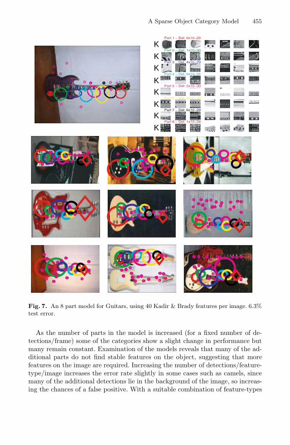
Fig. 7. An 8 part model for Guitars, using 40 Kadir & Brady features per image. 6.3%test error.

As the number of parts in the model is increased (for a fixed number of de-tections/frame) some of the categories show a slight change in performance butmany remain constant. Examination of the models reveals that many of the ad-ditional parts do not find stable features on the object, suggesting that morefeatures on the image are required. Increasing the number of detections/feature-type/image increases the error rate slightly in some cases such as camels, sincemany of the additional detections lie in the background of the image, so increas-ing the chances of a false positive. With a suitable combination of feature-types


Part 2 − Det: 3x10-30

Part 3 − Det: 1x10-30

Part 4 − Det: 2x10-30

Part 5 − Det: 7x10-30

Part 6 − Det: 3x10-32

Part 1 − Det: 3x10-30

C

H

C

C

H

H

Fig. 8. A 6 part model for Bottles, using a maximum of 20 Harris regions and 20Curves per image. 14.2% test error.

however, the increased number of parts and detections can give a more completecoverage of the object, improving performance (e.g. Cars (Rear) where the errordrops from 4.5% at 8 parts to 1.8% with 12 parts, using 40 detections/image ofall 3 feature types).

3.5 Complete Search Experiments

We now investigate the performance of feature-based recognition versus the com-plete approach. Taking the 8-part Cars (Rear) model shown in Figure 6, we applyit completely to the same test set resulting in the equal error rate dropping from


Fig. 9. A 10 part model for Houses, using 40 Kadir & Brady features per image. 16.5%test error.

4.5% to 1.8%. Detection examples for the complete approach are shown in Figure11, with the ROC curves for the two approaches shown in Figure 11(b).

The localization ability of the complete approach is tested on the Cars (Side)dataset, shown in Figure 10. A fully connected model (Figures 10 (a) & (b))was learnt and then decomposed into a star model and run completely overthe test set. An error rate of 7.8% was achieved – a decrease from the 11.5%obtained with a fully connected model using feature-based detection in [8]. Theperformance gain shows the benefits of using the complete approach despite theuse of a weaker shape model. Examples of the complete star model localizingmultiple object instances can be seen in Figure 10(c).


(a)

Part 1 − Det: 7x10−27

Part 2 − Det: 3x10−35

Part 3 − Det: 5x10−29

Part 4 − Det: 3x10−28

Part 5 − Det: 6x10−29

Part 6 − Det: 3x10−35

K

K

K

K

K

K

(b)

(c)

(d)

Fig. 10. (a) & (b) A 6 part model Cars (Side), learnt using Kadir & Brady features.(c) Examples of the model localizing multiple object instances by complete search.(d) Comparison between feature-based and complete localization for Cars (Side). Thesolid recall-precision curve is [1]; the dashed line is the fully connected shape modelwith feature-based detection [8] and the dotted line is the complete-search approachwith star model, using the model shown in (a) & (b). The equal error rate of 11.5%from [8] drops to 7.8% when using the complete search with the star model.


(a)

0 0.05 0.1 0.15 0.2 0.25 0.3 0.35 0.4 0.45 0.50.5

0.55

0.6

0.65

0.7

0.75

0.8

0.85

0.9

0.95

1

p(False Alarm)

p(D

ete

ctio

n)

(b)

Fig. 11. (a) Detection examples of the 8 part Cars (Rear) model from Figure 6 be-ing used completely. (b) ROC curves comparing feature-based (dashed) and completedetection (solid) for the 8 part Cars (Rear) model in Figure 6. Equal error improvesfrom 4.5% for feature-based to 1.8% for complete.

4 Summary and Conclusions

We have presented a heterogeneous star model. This model retains the impor-tant capabilities of the constellation model [8,21], namely that it is able to learnfrom unsegmented and unnormalized training data; and in recognition on unseenimages it is able to localize the detected model instance. The HSM outperforms


the constellation model on almost all of the six datasets presented in [8]. It isalso faster to learn, and faster to recognize (having O(NP ) complexity in recog-nition rather than the O(NP ) of the constellation model). We have also demon-strated the model on many other object categories varying over compactnessand shape. Note that while other models and methods have achieved superiorperformance to [8], for example [5,15,18,19], they are unable to both learn in aweakly-supervised manner and localize in recognition.

There are several aspects of the model that we wish to improve and investi-gate. Although we have restricted the model to a star topology, the approach isapplicable to a trees and k-fans [4], and it will be interesting to determine whichtopologies are best suited to which type of object category.

Acknowledgments

We are very grateful for suggestions from and discussions with Michael Isard,Dan Huttenlocher and Alex Holub. Financial support was provided by: ECProject CogViSys; EC PASCAL Network of Excellence, IST-2002-506778; UKEPSRC; Caltech CNSE and the NSF.

References

1. S. Agarwal and D. Roth. Learning a sparse representation for object detection.In Proceedings of the European Conference on Computer Vision, pages 113–130,2002.

2. E. Borenstein and S. Ullman. Class-specific, top-down segmentation. In Proceedingsof the European Conference on Computer Vision, pages 109–124, 2002.

3. M. Burl, T. Leung, and P. Perona. Face localization via shape statistics. In Int.Workshop on Automatic Face and Gesture Recognition, 1995.

4. D. Crandall, P. Felzenszwalb, and D. Huttenlocher. Spatial priors for part-basedrecognition using statistical models. In Proceedings of the IEEE Conference onComputer Vision and Pattern Recognition, San Diego, volume 1, pages 10–17,2005.

5. G. Csurka, C. Bray, C. Dance, and L. Fan. Visual categorization with bags ofkeypoints. In Workshop on Statistical Learning in Computer Vision, ECCV, pages1–22, 2004.

6. P. Feltzenswalb and D. Huttenlocher. Pictorial structures for object recognition.International Journal of Computer Vision, 61:55–79, January 2005.

7. R. Fergus and P. Perona. Caltech Object Category datasets.http://www.vision.caltech.edu/html-files/archive.html , 2003.

8. R. Fergus, P. Perona, and A. Zisserman. Object class recognition by unsupervisedscale-invariant learning. In Proceedings of the IEEE Conference on Computer Vi-sion and Pattern Recognition, June 2003.

9. R. Fergus, P. Perona, and A. Zisserman. A visual category filter for Google images.In Proceedings of the 8th European Conference on Computer Vision, Prague, CzechRepublic. Springer-Verlag, May 2004.

10. M. Fischler and R. Elschlager. The representation and matching of pictorial struc-tures. IEEE Transactions on Computer, 22(1):67–92, Jan. 1973.


11. C. J. Harris and M. Stephens. A combined corner and edge detector. In Proceedingsof the 4th Alvey Vision Conference, Manchester, pages 147–151, 1988.

12. F. Jurie and C. Schmid. Scale-invariant shape features for recognition of objectcategories. In Proceedings of the IEEE Conference on Computer Vision and PatternRecognition, Washington, DC, pages 90–96, 2004.

13. T. Kadir and M. Brady. Scale, saliency and image description. InternationalJournal of Computer Vision, 45(2):83–105, 2001.

14. Y. Ke and R. Sukthankar. PCA–SIFT: A more distinctive representation for localimage descriptors. In Proceedings of the IEEE Conference on Computer Visionand Pattern Recognition, Washington, DC, June 2004.

15. B. Leibe, A. Leonardis, and B. Schiele. Combined object categorization and seg-mentation with an implicit shape model. In Workshop on Statistical Learning inComputer Vision, ECCV, 2004.

16. D. Lowe. Local feature view clustering for 3D object recognition. In Proceedings ofthe IEEE Conference on Computer Vision and Pattern Recognition, Kauai, Hawaii,pages 682–688. Springer, December 2001.

17. P. Moreels, M. Maire, and P. Perona. Recognition by probabilistic hypothesisconstruction. In Proceedings of the 8th European Conference on Computer Vision,Prague, Czech Republic, pages 55–68, 2004.

18. A. Opelt, A. Fussenegger, and P. Auer. Weak hypotheses and boosting for genericobject detection and recognition. In Proceedings of the 8th European Conferenceon Computer Vision, Prague, Czech Republic, 2004.

19. J. Thureson and S. Carlsson. Appearance based qualitative image descriptionfor object class recognition. In Proceedings of the 8th European Conference onComputer Vision, Prague, Czech Republic, pages 518–529, 2004.

20. A. Torralba, K. P. Murphy, and W. T. Freeman. Sharing features: efficient boostingprocedures for multiclass object detection. In Proceedings of the IEEE Conferenceon Computer Vision and Pattern Recognition, Washington, DC, pages 762–769,2004.

21. M. Weber, M. Welling, and P. Perona. Unsupervised learning of models for recogni-tion. In Proceedings of the European Conference on Computer Vision, pages 18–32,2000.

lncs 4170 - a sparse object category model for …vgg/publications/2006/fergus06/fergus06.pdf · j....

Documents