lncs 3872 - document logical structure analysis …document logical structure analysis based on...

Document Logical Structure Analysis Basedon Perceptive Cycles

Yves Rangoni and Abdel Belaıd

Loria Research Center - Read Group, Vandœuvre-les-Nancy, France{rangoni, abelaid}@loria.fr

http://www.loria.fr/∼rangoni/http://www.loria.fr/∼abelaid/

Abstract. This paper describes a Neural Network (NN) approach forlogical document structure extraction. In this NN architecture, calledTransparent Neural Network (TNN), the document structure is stretchedalong the layers, allowing an interpretation decomposition from physi-cal (NN input) to logical (NN output) level. The intermediate layersrepresent successive interpretation steps. Each neuron is apparent andassociated to a logical element. The recognition proceeds by repetitiveperceptive cycles propagating the information through the layers. In caseof low recognition rate, an enhancement is achieved by error backpropa-gation leading to correct or pick up a more adapted input feature subset.Several feature subsets are created using a modified filter method. Thefirst experiments performed on scientific documents are encouraging.

1 Introduction

This paper tackles the problem of document logical structure extraction basedon physical feature observations within document images. Although this problemhas known many solutions, it still remains very challenging for noisy and variabledocuments.

The literature abounds of structure analysis approaches for different docu-ment classes. A survey of the most important approaches can be found in [1].Most of them are based on formal grammars describing the connection betweenlogical elements. However, these methods have drawbacks because the rules aregiven by the user and could be not sufficient to handle complex and noisy doc-uments. It is difficult to remove ambiguities and many thresholds must be fixedto process the matching between the physical and the logical structure.

Consequently, a learning-based method seems to be a more adapted solution.Artificial neural network (ANN) approaches allow such a training (rules arelearnt) and are known to be more robust to noise and deformation. However,ANN like the classical Multi Layer Perceptron (MLP) is considered as a blackbox and does not explicit the relationships between the neurons. In the sametime, domain-specific knowledge appears essential for document interpretationas mentioned in [2] and it seems useful to keep a part of knowledge in a DocumentImage Analysis (DIA) system.

H. Bunke and A.L. Spitz (Eds.): DAS 2006, LNCS 3872, pp. 117–128, 2006.c© Springer-Verlag Berlin Heidelberg 2006

118 Y. Rangoni and A. Belaıd

In order to take into account theses two aspects (knowledge and learning), wepropose a new ANN approach that use a Transparent Neural Network (TNN)architecture. This method has the same MLP capacities and can act, in the sametime, on the reasoning by introducing knowledge. The recognition task is doneprogressively by propagation of the inputs (local vision) towards the outputs(global vision). Back-propagation movements, during recognition step, are usedfor an input correction process as the human perception acts. These successive“perceptive cycles” (vision-interpretation) bring a context return which is veryhelpful for the input improvement.

This paper is organized as follows. In the first section, the TNN architectureis described. The second section details an input feature clustering method tospeed up the perceptive cycles. Finally, in the last section experimental resultsand discussions are reported.

2 The TNN Architecture Description

The proposed TNN architecture is described in Fig. 1. The first layer receivesphysical features where each element corresponds to a neuron. The followinglayers represent the logical structure at three different levels, from fine to coarse(see Fig.8 for the whole input and output names).

All the layers are fully connected and all the neurons carry interpretableconcepts. This modeling integrates common knowledge on “general” document

SemanticFeatures

Numerical/TextIndent

KeywordEnumeration

…

GeographicalFeatures

LineImageText

PositionSize

Spacing…

Logicalstructure

Main titleAuthor

AbstractDivision

…CopyrightAlgorithmSummary

Logicalelements

TitleCaption

FootNoteParagraph

ListEnumeration

TableBibliography

Float

Structural

PictureSchemaFormula

TextLineBox

Row of cellsColumn of cells

Physical level Logical level

Second layer(21 neurons) Third layer Fourth layer

Input layer(56 neurons)

MorphologicalFeatures

Font sizeBoldItalic

UnderlineColor…

Fig. 1. Neuron semantic for document analysis

Document Logical Structure Analysis Based on Perceptive Cycles 119

structure. It can be more precise if a DTD (Document Type Definition) is givenas the DTD organizes the logical element in hierarchy. The real TNN output isthe first logical level (the second layer) while the last layers represent the globalcontext (third and fourth layers). They are used to precise the context which isneeded for logical structure identification during the perceptive cycles.

This system can be considered as a hybrid method set between a model-driven (DTD integration) and a data-driven approach (training phase). As for aclassical MLP, a database is used to train the links between physical and finallogical structures. The list of input and output elements is given in Fig. 8.

As the model is transparent and errors can be known for each output layers,the training of the whole network is achieved locally for each consecutive layerpairs. The weight modifications are carried out by an error correction principle.The first stage consists in initializing the weights with random values, thenfor each couple (Input, Output) of the training database, a predicted value iscomputed by propagation. The error between the computed output P and thedesired output O is then determined. The second stage back-propagates thiserror in the previous layers. If the activation function is a sigmoid, the value toadd to a weight wi,j is α(Oj − Pi)Pi(1 − Pj)Ii.

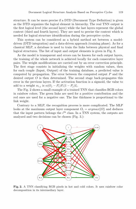
The Fig. 2 shows a small example of a trained TNN that classifies RGB colorsin rainbow colors. The green links are used for a positive contribution and thered ones are used for a negative one. The line thickness is proportional to thelink weight.

Contrary to a MLP, the recognition process is more complicated. The MLPlooks at the maximum output layer component Oi = argmax{O} and deducesthat the input pattern belongs the ith class. In a TNN system, the outputs areanalyzed and two decisions can be chosen (Fig. 3.):

Fig. 2. A TNN classifying RGB pixels in hot and cold colors. It uses rainbow colordecomposition in its intermediary layer.


Xn

X2

X1

An

A2

A1

Inputs Outputs

Context

Ambiguity?

Initialpattern

database

« Mean » Selection

E1 E2 E3 E4

Representative samples by classes

Pattern is recognized

No

Correct inputs

• Context information• Input pattern expected• Re-tune algorithm

Input sample

Yes

Documentimage

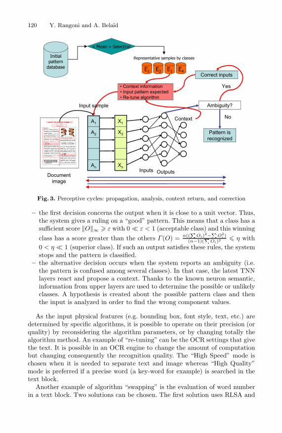
Fig. 3. Perceptive cycles: propagation, analysis, context return, and correction

– the first decision concerns the output when it is close to a unit vector. Thus,the system gives a ruling on a “good” pattern. This means that a class has asufficient score ‖O‖∞ � ε with 0 � ε < 1 (acceptable class) and this winningclass has a score greater than the others Γ (O) = n((

�Oi)2−

�O2

i )(n−1)(

�Oi)2

� η with0 < η � 1 (superior class). If such an output satisfies these rules, the systemstops and the pattern is classified.

– the alternative decision occurs when the system reports an ambiguity (i.e.the pattern is confused among several classes). In that case, the latest TNNlayers react and propose a context. Thanks to the known neuron semantic,information from upper layers are used to determine the possible or unlikelyclasses. A hypothesis is created about the possible pattern class and thenthe input is analyzed in order to find the wrong component values.

As the input physical features (e.g. bounding box, font style, text, etc.) aredetermined by specific algorithms, it is possible to operate on their precision (orquality) by reconsidering the algorithm parameters, or by changing totally thealgorithm method. An example of “re-tuning” can be the OCR settings that givethe text. It is possible in an OCR engine to change the amount of computationbut changing consequently the recognition quality. The “High Speed” mode ischosen when it is needed to separate text and image whereas “High Quality”mode is preferred if a precise word (a key-word for example) is searched in thetext block.

Another example of algorithm “swapping” is the evaluation of word numberin a text block. Two solutions can be chosen. The first solution uses RLSA and


(a)

(b)

(c) (d)

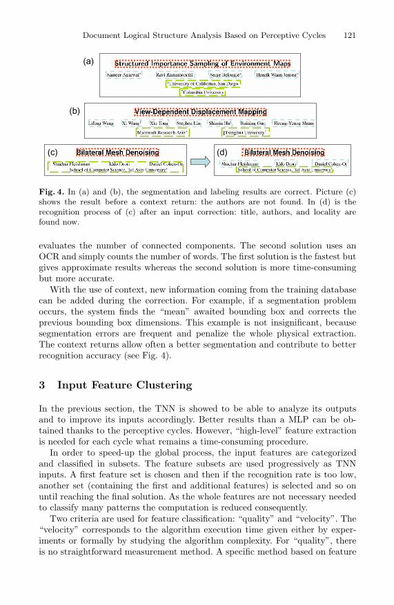
Fig. 4. In (a) and (b), the segmentation and labeling results are correct. Picture (c)shows the result before a context return: the authors are not found. In (d) is therecognition process of (c) after an input correction: title, authors, and locality arefound now.

evaluates the number of connected components. The second solution uses anOCR and simply counts the number of words. The first solution is the fastest butgives approximate results whereas the second solution is more time-consumingbut more accurate.

With the use of context, new information coming from the training databasecan be added during the correction. For example, if a segmentation problemoccurs, the system finds the “mean” awaited bounding box and corrects theprevious bounding box dimensions. This example is not insignificant, becausesegmentation errors are frequent and penalize the whole physical extraction.The context returns allow often a better segmentation and contribute to betterrecognition accuracy (see Fig. 4).

3 Input Feature Clustering

In the previous section, the TNN is showed to be able to analyze its outputsand to improve its inputs accordingly. Better results than a MLP can be ob-tained thanks to the perceptive cycles. However, “high-level” feature extractionis needed for each cycle what remains a time-consuming procedure.

In order to speed-up the global process, the input features are categorizedand classified in subsets. The feature subsets are used progressively as TNNinputs. A first feature set is chosen and then if the recognition rate is too low,another set (containing the first and additional features) is selected and so onuntil reaching the final solution. As the whole features are not necessary neededto classify many patterns the computation is reduced consequently.

Two criteria are used for feature classification: “quality” and “velocity”. The“velocity” corresponds to the algorithm execution time given either by exper-iments or formally by studying the algorithm complexity. For “quality”, thereis no straightforward measurement method. A specific method based on feature


nm

m

m

n x

x

x

x

x

x

2

1

1

21

11

m vectors Xi in Rn

nnn

n

rr

r

rrr

1

21

11211

Correlation matrix CRMat

n000

00

00

000

2

1

nnn vv

v

vv

1

21

1211

nnn vv

v

vv

1

21

1211

=

T

ViVi Vi

ViVi

Vi

Vi Vi

Clusterize Vi

13 2

Chosethe best

xi

Chose the secondbest xi

…

EigenvectorMatrix

EigenvectorMatrix

EigenvalueMatrix

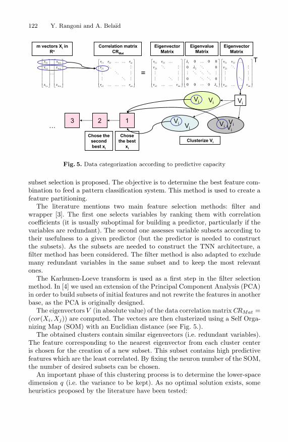
Fig. 5. Data categorization according to predictive capacity

subset selection is proposed. The objective is to determine the best feature com-bination to feed a pattern classification system. This method is used to create afeature partitioning.

The literature mentions two main feature selection methods: filter andwrapper [3]. The first one selects variables by ranking them with correlationcoefficients (it is usually suboptimal for building a predictor, particularly if thevariables are redundant). The second one assesses variable subsets according totheir usefulness to a given predictor (but the predictor is needed to constructthe subsets). As the subsets are needed to construct the TNN architecture, afilter method has been considered. The filter method is also adapted to excludemany redundant variables in the same subset and to keep the most relevantones.

The Karhunen-Loeve transform is used as a first step in the filter selectionmethod. In [4] we used an extension of the Principal Component Analysis (PCA)in order to build subsets of initial features and not rewrite the features in anotherbase, as the PCA is originally designed.

The eigenvectors V (in absolute value) of the data correlation matrix CRMat =(cor(Xi, Xj)) are computed. The vectors are then clusterized using a Self Orga-nizing Map (SOM) with an Euclidian distance (see Fig. 5.).

The obtained clusters contain similar eigenvectors (i.e. redundant variables).The feature corresponding to the nearest eigenvector from each cluster centeris chosen for the creation of a new subset. This subset contains high predictivefeatures which are the least correlated. By fixing the neuron number of the SOM,the number of desired subsets can be chosen.

An important phase of this clustering process is to determine the lower-spacedimension q (i.e. the variance to be kept). As no optimal solution exists, someheuristics proposed by the literature have been tested:


– fixed number q: this is a straightforward method where cutting level is im-posed by the user.

– fixed percentage: similarly to the previous case, but here the user choosesthe first p% of the eigenvalues.

– cumulated percentage: the number q is determined when the sum of the firstvariance (eigenvalue) is greater than a given fixed percentage.

These three methods are usual but their choice assumes that the user over-comes its application and can appreciate the dimension to use. These methodsare often used in social sciences because it is easier to interpret the data. Twoother methods, which are more general and more robust, are based on the shapeof the eigenvalue sequence:

– Kaiser method: the average of all the variances is calculated. The spacedimension q is determined when the sum of the first variance is greater thanthis average. Of a wide spread employment, it can be put at fault.

– Cattell method: [5] suggests to find the place where the smooth decrease ofeigenvalues appears to level off to the right of the plot (the scree-test). Thisheuristic is often considered as the most powerful [6]

4 Experimental Results and Discussion

Before introducing results on document image analysis, experiments about “low-level” and highly correlated features are presented.

A first experimentation procedure is employed to illustrate the variable subsetcreation method. For this purpose, the MNIST database [7] is used. A MultiLayerPerceptron is used to evaluate the group validity. This classifier has the samesettings along all the experiments (topology, initial random weights, etc.). Twoexperiments have been made on this database. The first uses the whole initialpixels of each image (digits are 28×28 pixel images). The second experiment usesresampled images (in a 7×7 format). Thus, we have for the first experiment 784variables are considered in the first experiment and 49 for the second one.

The MLP is trained with different variable subsets and the recognition rate ischosen as a quality measurement. The subsets are compared to randomly createdones. One thousand of random subsets have been generated and evaluated bythe MLP. Then the best one is retained for the comparison. This procedure willbe the same for the following experiments about document analysis.

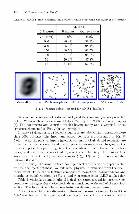
Table 1 shows normalized comparison results between the subset obtained byour method and the best of the random subsets for the initial MNIST database.The Fig. 6 shows the position of the selected pixels in the image. The first picturerepresents the “mean” digit coming from the whole database ( 1

n

∑ni=1 Ii) and in

the next three pictures, chosen pixels can be seen. The Table 2 is similar to theTable 1 but here 7×7 pixel images are used for test.

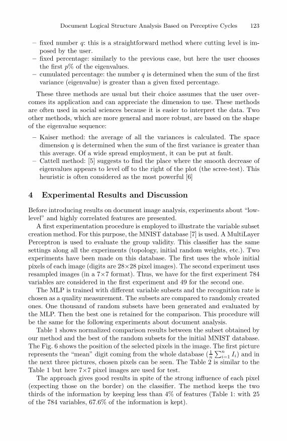
The approach gives good results in spite of the strong influence of each pixel(expecting those on the border) on the classifier. The method keeps the twothirds of the information by keeping less than 4% of features (Table 1: with 25of the 784 variables, 67.6% of the information is kept).


Table 1. MNIST digit classification accuracy while decreasing the number of features

Method# features Random Our selection

784(max) 100% 100%500 98.4% 99.2%300 95.9% 98.4%150 90.5% 96.5%100 84.2% 94.2%50 70.9% 87.8%25 47.1% 67.6%

Mean digit image 25 chosen pixels 50 chosen pixels 100 chosen pixels

Fig. 6. Feature subsets created for MNIST database

Experiments concerning the document logical structure analysis are presentedbelow. We have chosen as a main database 74 Siggraph 2003 conference papers[8]. The documents are scientific articles having many and diversified logicalstructure elements (see Fig. 7 for two examples).

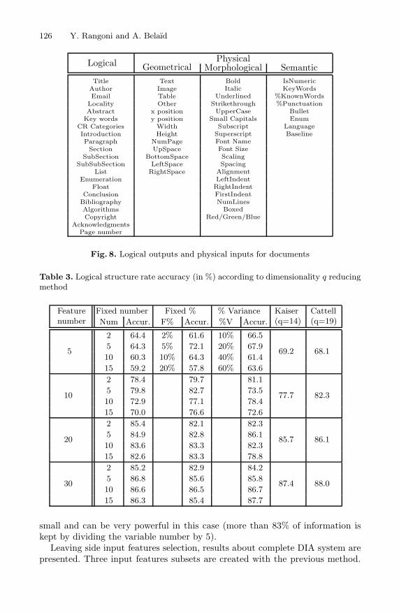
In these 74 documents, 21 logical structures are labeled that represents morethan 2000 patterns. The input and output features are presented in Fig. 8.Note that all the physical inputs (geometrical, morphological, and semantic) arenumerical values between 0 and 1 after possibly normalization. In general, thenumber represents a percentage (e.g. the percentage of bold characters in a textblock) and for other features that represent a number (e.g. the number k ofkeywords in a text block) we use the series

∑kn=1 1/(n + 1) to have a number

between 0 and 1.As previously, the same protocol for input feature selection is experimented

on this document database. We extracted physical information from the docu-ment layout. There are 56 features composed of geometrical, typographical, andmorphological information (see Fig. 8) and we use once again a MLP as classifier.

Table 3 synthesizes some results of logical structures recognition accuracy ac-cording to the eigenvalue choice methods as mentioned at the end of the previoussection. The five methods have been tested on different subset sizes.

The choice of the space dimension influences the results quality. Even if theMLP is a classifier able to give good results with few features, choosing too low


Table 2. Resampled MNIST digit classification accuracy while decreasing the numberof features


49(max) 100% 100%35 94.2% 99.3%25 81.2% 88.6%15 56.2% 70.5%10 43.9% 55.2%

Permission to make digital/hard copy of part of all of this work for personal orclassroom use is granted without fee provided that the copies are not made ordistributed for profit or commercial advantage, the copyright notice, the title of thepublication, and its date appear, and notice is given that copying is by permissionof ACM, Inc. To copy otherwise, to republish, to post on servers, or to redistributeto lists, requires prior specific permission and/or a fee.© 2003 ACM 0730-0301/03/0700-0651 $5.00

Interactive Boolean Operations on Surfel-Bounded Solids

Bart Adams∗ Philip Dutre∗

Department of Computer ScienceKatholieke Universiteit Leuven

Abstract

In this paper we present an algorithm to perform interactive booleanoperations on free-form solids bounded by surfels. We introducea fast inside-outside test to check whether surfels lie within thebounds of another surfel-bounded solid. This enables us to add,subtract and intersect complex solids at interactive rates. Our algo-rithm is fast both in displaying and constructing the new geometryresulting from the boolean operation.We present a resampling operator to solve problems resulting

from sharp edges in the resulting solid. The operator resamples thesurfels intersecting with the surface of the other solid. This enablesus to represent the sharp edges with great detail.We believe our algorithm to be an ideal tool for interactive edit-

ing of free-form solids.

CR Categories: I.3.5 [Computer Graphics]: ComputationalGeometry and Object Modeling—Curve, surface, solid, and ob-ject representations; I.3.6 [Computer Graphics]: Methodology andTechniques—Graphics data structures and data types I.3.4 [Com-puter Graphics]: Graphics Utilities—Graphics editors

Keywords: free-form modeling, boolean operations, surfels,point-based geometry

1 Introduction

Constructive solid geometry (CSG) has been a useful tool in com-puter graphics for many years. Usually, CSG is applied to primitiveobjects (spheres, cylinders, cubes) to construct objects with a morecomplex geometric shape. However, boolean operations are also aversatile tool for editing free-form solids. Adding, subtracting andintersecting solids enables us to create more complex models. Inthis paper we present boolean operations as an intuitive and inter-active editing tool for free-form solids bounded by surfels. Surfels,represented as oriented points in 3D space, approximate the localorientation of the surface they represent. Each surfel can be con-sidered to represent a small area of this surface. As a consequence,when performing boolean operations on two solids A and B, mostof the surfels of the surface of solid A are completely inside or out-side solid B and vice versa. Only a small number of surfels intersectwith the surface of the other solid.Our algorithm works in two steps: in a first step we classify the

surfels of both solids as inside, outside or intersecting with the sur-

∗email:{barta,phil}@cs.kuleuven.ac.be

Figure 1: Two free-form surfel-bounded solids constructed usingCSG (inspired by ”Bond of Union” by M.C. Escher).

face of the other solid. In a second step we resample the surfelsintersecting with the surface of the other solid. Our method is fast,both in displaying the boolean operations as in calculating the newgeometry of the resulting solid. An example of a free-form surfel-bounded solid constructed with our algorithm is shown in figure 1.This paper addresses the following important questions:

• How to test efficiently whether a surfel of one surfel-boundedsolid lies inside or outside another surfel-bounded solid?

• How to represent the sharp edges typically resulting from per-forming boolean operations on solids, using surfels?

We start by giving a brief overview of related work in section 2.Section 3 introduces the concepts related to surfel-bounded solids.In section 4 we present a fast inside-outside test that enables usto classify the surfels of solid A as inside, outside or intersectingwith the surface of solid B. In section 5 we consider the surfelsintersecting with the surface of the other solid and propose the fastresampling operator. Section 6 gives implementation details andillustrates that we are able to perform boolean operations on com-plex solids at interactive rates. We conclude and give some topicsof future research possibilities in section 7.

2 Related Work

Point-Based Geometry

The interest in using points as a display primitive in com-puter graphics has grown tremendously in recent years. Pfisteret al. [2000] introduced the concept of surfels inspired by thework of Levoy and Whitted [1985], and more recently the workof Grossman and Dally [1998]. Significant research has beenperformed on efficient high quality rendering of point-basedgeometry. QSplat [Rusinkiewicz and Levoy 2000] uses a hierarchyof bounding spheres for progressive rendering of large models.Zwicker et al. [2001] introduce surface splatting which makesthe benefits of the Elliptical Weighted Average (EWA) filteravailable to point-based rendering. Alexa et al. [2001] presentpoint set surfaces and use down-sampling and up-sampling tomeet the required display quality. Kalaiah and Varshney [2001]

651

(a) (b) (c) (d) (e)

Figure 3: Density in plane space. (a) Scene with face f and its three vertices highlighted. (b) Set of planes going through each vertex.represented in plane space. The plane of f corresponds to the intersection of the three sheets. (c) Validity domain of each vertex. (d)Discretized validity domain of f . (e) Coverage for the whole house. We clearly see 6 maxima (labelled) corresponding to the 4 side faces andthe 2 sides of the roof. Note in addition the degenerate maximum that spans a whole row for φ � π � 2. All values of θ match the same plane:the plane of the ground.

}

j

}

i

}

k

Figure 4: Rasterization in plane space.

Greedy (input model, threshold ε)set of faces F =input modelbillboard cloud BC = /0while F �� /0

Pick bin B with highest densityCompute validF

ε � B �Pi = RefineBin (B , validF

ε � B � )UpdateDensity(validF

ε � Pi � )F = F � validF

ε � Pi �BC = BC � Pi

Compute textures(BC )

Figure 5: Pseudocode of the greedy selection of planes.

3 Greedy optimization

Now that we have defined and computed a density over plane space,we present our greedy optimization approach to select a set ofplanes that approximate the input model. We iteratively pick thebin with the highest density. We then search for a plane in the binthat can collapse the corresponding set of valid faces. This may re-quire an adaptive refinement of the bin in plane space as explainedbelow. Once a plane is found, we update the density to remove thecontribution and penalty due to the collapsed faces, and proceed tothe next highest-density bin. Once all the faces have been collapsed,we compute the corresponding textures on each plane.

3.1 Adaptive refinement in plane space

Our grid only stores the simple density d�B of each bin, and for

memory usage reasons, we do not store the corresponding set offaces validε

�B . We iterate on the faces that have not yet been col-

lapsed to compute those that are valid for B. Further computationsfor the plane refinement are performed using only this subset of themodel. We note quantities such as density or validity set restrictedto such a subset of faces F with the superscript F .

Recall that the density stored in our plane-space grid uses thesimple validity, and that the faces that are simply valid for a bin arenot necessarily valid for all its planes. We therefore need to refineour selection of a bin to find the densest plane. We subdivide bins

RefineBin (bin B , set of faces F )plane P = center of Bif (validF

ε � P � � � validFε � B � )

return Pbin Bmax=NULLfor each of the 27 neighbors Bi of B

Subdivide Bi into 8 sub-bins Bi j

for each Bi j // there is a total of 8*27 such Bi j

Compute dF � Bi j �if (dF � Bi j � � dF � Bmax � )

Bmax� Bi j

return RefineBin (Bmax , validFε � Bmax � )

Figure 6: Pseudo-code of recursive adaptive refinement in planespace.

adaptively until the plane at the center of a sub-bin is valid for theentire validity set of the sub-bin (Fig. 6).

We allow the refinement process to explore the neighbors of thebin as well. Indeed, because we use simple validity, the densestplane can be slightly outside the bin we initially picked, as illus-trated by figure 7. We use a simple strategy: We subdivide the binand its 26 neighbors, and pick among these 27 8 sub-bins, the onewith highest simple density.

valid(f2)valid(f2)

valid(f3)

B1 B2P

Figure 7: Simple density in plane space. Although bin B1 has max-imum simple density, the densest plane is P , which is in bin B2.

Bins are then updated to remove the contributions and penaltiesof the collapsed faces. We iterate over the faces collapsed on thenew plane and use the same procedure described in Section 2.4,except that contributions and penalties are removed. The algorithmthen proceeds until all faces of the model are collapsed on planes.

3.2 Computing textures

Each plane Pi is assigned a set of collapsed faces validFε

�Pi during

the greedy phase. We first find the minimum bounding rectangle ofthe projection of these faces in the texture plane (using the CGALlibrary[CGA n. d.]), then we shoot a texture by rendering the faces

692

Fig. 7. Two scientific document database samples

or too high eigenvector dimension can be bad for the input feature clusteringand consequently for the classifier.

It seems here (and for other tests that have be done on MNIST) that theCattell method (that set q = 19) is most of the time better than Kaiser (withq = 14). The two methods, which automatically find the number q, give the sameor better results than the classical ones where the user must fix this number. Wewill retain for the following tests the Cattell method that seems to be the mostrobust on many experimentations.

As expected and confirmed in Table 4, these “high-level” features lends wellto this selection.

In this case, the choice of a small set of features is more difficult. The featureclustering method seems to be appropriate when the number of features is rather


Logical PhysicalGeometrical Morphological Semantic

Title Text Bold IsNumericAuthor Image Italic KeyWordsEmail Table Underlined %KnownWords

Locality Other Strikethrough %PunctuationAbstract x position UpperCase Bullet

Key words y position Small Capitals EnumCR Categories Width Subscript LanguageIntroduction Height Superscript BaselineParagraph NumPage Font Name

Section UpSpace Font SizeSubSection BottomSpace Scaling

SubSubSection LeftSpace SpacingList RightSpace Alignment

Enumeration LeftIndentFloat RightIndent

Conclusion FirstIndentBibliography NumLinesAlgorithms BoxedCopyright Red/Green/Blue

AcknowledgmentsPage number

Fig. 8. Logical outputs and physical inputs for documents

Table 3. Logical structure rate accuracy (in %) according to dimensionality q reducingmethod

Featurenumber

Fixed number Fixed % % Variance Kaiser(q=14)

Cattell(q=19)Num Accur. F% Accur. %V Accur.

5

2 64.4 2% 61.6 10% 66.5

69.2 68.15 64.3 5% 72.1 20% 67.910 60.3 10% 64.3 40% 61.415 59.2 20% 57.8 60% 63.6

10

2 78.4 79.7 81.1

77.7 82.35 79.8 82.7 73.510 72.9 77.1 78.415 70.0 76.6 72.6

20

2 85.4 82.1 82.3

85.7 86.15 84.9 82.8 86.110 83.6 83.3 82.315 82.6 83.3 78.8

30

2 85.2 82.9 84.2

87.4 88.05 86.8 85.6 85.810 86.6 86.5 86.715 86.3 85.4 87.7

small and can be very powerful in this case (more than 83% of information iskept by dividing the variable number by 5).

Leaving side input features selection, results about complete DIA system arepresented. Three input features subsets are created with the previous method.


Table 4. Logical elements classification accuracy while decreasing the number of fea-tures


56(max) 100% 100%35 86.9% 99.3%25 65.0% 79.6%15 51.8% 80.1%10 35.1% 83.8%5 17.9% 44.9%

Table 5. Logical classification by MLP and TNN with perceptive cycles

Recognition TNNrates MLP C1 C2 C3 C4

All elements 81.6% 45.2 78.9 90.2 91.7%Best class 86.9% 66.7 85.3 85.3 99.3%

Worst class 0.0% 0.0 0.0 4.0 28.6%

Recognition time(MLP as reference)

100% 70% 145% 185% 240%

Extraction tools, which can be configured, are used to extract the physical layout.During the recognition phase, the system can choose between the feature subsetsand act on extraction tools as mentioned in Section 3. The training stage uses44 documents and 30 for the test. Test results between a MLP and the TNN atthe end of four perceptive cycles are presented in Fig.5.

The perceptive cycles increase the recognition rates. After 4 cycles, the clas-sifier reaches 91.7%. A TNN without perceptive cycles is worse than a MLP(45.2% instead of 81.6%) because TNN does not have many constraints in itsintermediate layers. With perceptive cycles, the context returns make it possibleto gain in precision while the algorithm complexity increases with a 2.5 factor.

5 Conclusion

We presented in this article a neural network architecture for document logicalstructure analysis. The method uses a Transparent Neural Network that makes itpossible to introduce knowledge in each neuron and to organize in hierarchy theneurons in order to create a “vision” decomposition. The topology can simulatea decomposition hierarchy from fine (the patterns to recognized) to coarse (theglobal context).


Thanks to this system, we can adapt the computation time according tothe pattern granularity and complexity. These“perceptive cycles” as named incognitive psychology allow simulating in the same system a recognition pro-cess that uses automatic and fixed knowledge rules, a hierarchical view, and aninterpretation-correction process thanks to hypothesis creation. An input featureclustering was done to speed-up the perceptive cycles.

The TNN gives encouraging results. Although some improvements are inhand, tests are already better than a simple MLP, without adding too heavycomputation. In our future works, we will propose a genetic-method to chooserepresentative samples in the database during the context return. Another workwill be done to improve the feature subset creation and a method to deal withthe final cases of rejected patterns will be presented.

References

1. Mao, S., Rosenfelda, A., Kanungo, T.: Document structure analysis algorithms: Aliterature survey. SPIE Electronic Imaging (2003)

2. Nagy, G.: Twenty years of document image analysis in pami. PAMI (2000)3. Guyon, I., Elisseeff, A.: An introduction to variable and feature extraction. Journal

of Machine Learning Research (2003)4. Rangoni, Y., Belaıd, A.: Data categorization for a context return applied to logical

document structure recognition. ICDAR (2005)5. Cattell, R.: The scree test for the number of factors. Multivariate Behavioral

Research (1966)6. Zwick, W.R., Velicer, W.F.: Comparison of five rules for determining the number

of components to retain. Psychological Bulletin (1986)7. LeCun, Y.: (http://yann.lecun.com/exdb/mnist/)8. Siggraph: http://www.siggraph.org/s2003/. (2003)

lncs 3872 - document logical structure analysis …document logical structure analysis based on...

Documents