lm10 system manual - university of minnesota · analysis system & nta 1.5 ... except as limited...
TRANSCRIPT

Doc No 001010151a 1
NanoSight LM10 Nanoparticle Analysis System & NTA 1.5
Analytical Software
Operating Manual
© 2008 NanoSight Ltd. 2 Centre One, Lysander Way, Old Sarum Business Park Salisbury SP4 6BU UK
Tel: 01722 349439 Fax: 01722 329640 email [email protected] Web site www.nanosight.co.uk
The information in this Operating Manual correct Feb 2008. Our instruments are continually being developed.
Consequently, we reserve the right to alter the information without prior notice. Ver 1.51a (Feb 2008)

© 2007 NanoSight Ltd. 2 Centre One, Lysander Way, Old Sarum Business Park Salisbury SP4 6BU UK Tel: 01722 349439, Fax: 01722 329640, email [email protected], web www.nanosight.co.uk
Page 2 of 68
Contents
1. IMPORTANT NOTES ................................................................................................................... 4
A. USAGE ........................................................................................................................................... 4
B. SAFETY.......................................................................................................................................... 4
SERVICING............................................................................................................................................. 5
C. HANDLING ..................................................................................................................................... 5
D. WARRANTY ................................................................................................................................... 5
E. TECHNICAL SPECIFICATION OF LM VIEWING UNIT......................................................................... 5
F. UNPACKING AND INITIAL INSPECTION ........................................................................................... 6
G. RETURNING EQUIPMENT ............................................................................................................... 6
H. MAINTENANCE .............................................................................................................................. 6
I. DEVICE LAYOUT ............................................................................................................................ 7
J. SCHEMATIC AND PARTS LIST ........................................................................................................ 8
2. BASIC INTRODUCTION TO TECHNIQUE ............................................................................. 9
3. SAMPLE PREPARATION AND DISPERSION ...................................................................... 11
A. INTRODUCTION ............................................................................................................................ 11
B. SUSPENDING SOLVENT ................................................................................................................ 11
C. PARTICLE SIZE RANGE APPLICABLE ............................................................................................ 11
D. PARTICLE CONCENTRATION ......................................................................................................... 12
E. DILUTION .................................................................................................................................... 12
F. PHYSICAL REMOVAL OF LARGE PARTICLES ................................................................................. 12
Filtration ........................................................................................................................................ 12
Centrifugation................................................................................................................................. 12
Settling ............................................................................................................................................ 12
G. DISPERSION AND DEAGGLOMERATION ........................................................................................ 13
Typical Examples of Dispersants .................................................................................................... 13
4. MICROSCOPE SET-UP ............................................................................................................. 15
A. MICROSCOPE ............................................................................................................................... 15
B. TRINOCULAR HEAD LEVERS ......................................................................................................... 16
C. MICROSCOPE USAGE .................................................................................................................... 16
5. LM10 USAGE ............................................................................................................................... 17
A. ASSEMBLING THE LM SAMPLE UNIT ........................................................................................... 17
B. INJECTION INTO THE LM UNIT .................................................................................................... 17
C. ADJUSTING THE MICROSCOPE ..................................................................................................... 18
D. VIEW OR CAPTURE IMAGES ......................................................................................................... 18
E. LOADING A NEW SAMPLE ............................................................................................................ 18
F. CLEANING ................................................................................................................................... 18
G. STORAGE ..................................................................................................................................... 19
6. NTA SOFTWARE USAGE ......................................................................................................... 20
A. AIM ............................................................................................................................................. 20
B. SYSTEM REQUIREMENTS ............................................................................................................. 20
C. START-UP.................................................................................................................................... 20
D. IMAGE CAPTURE ......................................................................................................................... 20
E. IMAGE PROCESSING ..................................................................................................................... 24
F. BATCH CAPTURE AND PROCESS .................................................................................................. 31
Batch Capture ................................................................................................................................. 32
Batch Process ................................................................................................................................. 32
G. OUTPUT PARAMETERS ................................................................................................................. 34
Screen display ................................................................................................................................. 34
Graphical Output Scales ................................................................................................................ 34
Cumulative Undersize and Oversize ............................................................................................... 35
Report ............................................................................................................................................. 35
Screenshot ...................................................................................................................................... 36

© 2007 NanoSight Ltd. 2 Centre One, Lysander Way, Old Sarum Business Park Salisbury SP4 6BU UK Tel: 01722 349439, Fax: 01722 329640, email [email protected], web www.nanosight.co.uk
Page 3 of 68
Export Data .................................................................................................................................... 36
7. WORKED EXAMPLES .............................................................................................................. 41
200 nm Reference Latex Spheres .................................................................................................... 41
100 nm Reference Latex Spheres .................................................................................................... 47
300 nm Reference Latex Spheres .................................................................................................... 50
400 nm Reference Latex Spheres .................................................................................................... 53
30 nm Gold Colloid ........................................................................................................................ 55
Poly-Dispersed Sample of 100 nm and 200 nm Polystyrene Reference Spheres ............................ 58
H. RECOMMENDED CAPTURE AND ANALYSIS SETTINGS ................................................................... 61
8. FREQUENTLY ASKED QUESTIONS...................................................................................... 62
A. FUNDAMENTAL QUESTIONS ......................................................................................................... 62
How much light is scattered by a particle? .................................................................................... 62
How long is a sample stable for? Will the nanoparticles aggregate? ............................................ 62
The particles are only being imaged in two dimensions, but they must be moving in three
dimensions. Is this a problem? ....................................................................................................... 63
How does a larger particle (such as an advanced agglomerate or contaminant) affect the
measurement? ................................................................................................................................. 63
Can I use different solvents in your device? ................................................................................... 63
What is the upper size limit of particles that can be sized by your system?.................................... 63
What is the smallest particle that can be analysed? ....................................................................... 63
Why do my particles twinkle and appear to diffuse asymmetrically? ............................................. 64
What is the best particle concentration to use? .............................................................................. 64
B. VALIDITY OF METHOD ................................................................................................................. 64
How accurately can particle size be determined? .......................................................................... 64
Are there enough particles in my analysis? .................................................................................... 64
Why do you not use an increased frame rate to obtain more data? ............................................... 65
How well can different sizes be resolved from each other in a mixture? ....................................... 65
How reproducible is the result? ..................................................................................................... 65
Can you use NanoSight system to obtain concentration measurement? ......................................... 65
Small particles are not tracked as long as large particles. Is this a problem? ............................... 65
C. USER QUESTIONS ......................................................................................................................... 66
How wide a range of particle sizes can be analysed at the same time? ......................................... 66
How do I calibrate my system? ....................................................................................................... 66
How long does the sample temperature take to equilibrate?.......................................................... 66
I am still seeing a significant flow of particles, but have waited longer than 30s. Why is this? ..... 66
Small particles are not as bright as large particles and I find it hard to track both at the same
time, what should I do?................................................................................................................... 67
I want to put my movies in a presentation but they are very large. Can I compress these? ........... 67
Is it possible I could have blocked the inlet outlet ports with particles? ........................................ 67
D. SPECIFICATION QUESTIONS .......................................................................................................... 67
What are the space requirements of the system? ............................................................................ 67
What are the dimensions of the sample chamber?.......................................................................... 67
How long is the lifetime of laser source in LM10 unit? .................................................................. 67
How long can I leave a sample in the cell? .................................................................................... 67
Is the system safe? .......................................................................................................................... 67
What is the unit made of? ............................................................................................................... 68
Do I need an anti-vibration table for the system? .......................................................................... 68
9. TROUBLESHOOTING AND FAULT FINDING ..................................................................... 68

© 2007 NanoSight Ltd. 2 Centre One, Lysander Way, Old Sarum Business Park Salisbury SP4 6BU UK Tel: 01722 349439, Fax: 01722 329640, email [email protected], web www.nanosight.co.uk
Page 4 of 68
1. Important Notes a. Usage
The NanoSight LM10 device has been designed to be used only in conjunction with and mounted on the optical microscope supplied.
b. Safety While the NanoSight LM10 device is classified (to BS EN 60825-1 (2001)) as a Class1 laser device, it is very important that the following instructions are adhered to.
! CAUTION – USE OF CONTROLS OR ADJUSTMENTS OR PERFORMANCE OF
PROCEDURES OTHER THAN THOSE SPECIFIED HEREIN MAY RESULT IN HAZARDOUS RADIATION EXPOSURE
• The instrument contains a Class 3B laser source which must never be removed from the main instrument housing.
• The laser aperture is located in the recess in the LM12 where the glass flat sits (see page 7).
• The device should never be switched on without the optical element and top plate being secured in position.
• The torque screws supplied to hold the top plate in place must be in position and tightened prior to turning on the laser power.
• Laser power must be turned off prior to removing the top-plate torque screws with the adapter on the power supply that is supplied.
• ! On loading the LM10 unit with sample via a syringe, it is occasionally possible to
inadvertently introduce bubbles into the path of the laser beam resulting in a degree of specular reflection. The introduction or formation of bubbles can be minimised by careful introduction of sample in which the liquid is introduced as slowly as possible while the unit is tilted to allow bubbles to escape from the outlet port. If bubbles are present, they can be visually recognised as bright light scattering centres in the beam path when the unit is being loaded. It is very important that such bubble be removed, by flushing with further sample, before the beam is viewed via the microscope oculars.
• Similarly, certain samples may generate bubbles through out-gassing of dissolved gases over extended periods. In both cases, the image collected by the CCD camera supplied will show a high intensity region (or may be completely saturated) indicative of the presence of such bubbles. Before viewing the beam via the microscope oculars, such bubbles must be removed by carefully withdrawing the sample and slowly reintroducing it to allow the bubbles to disperse. If samples repeatedly show evidence of bubble formation, it is advisable to de-gas the sample before analysis.
• The instrument must not be used in hazardous areas.
• It is the responsibility of the operator to determine the requisite protection for each application.
• Use only the accessories supplied with the instrument.
• Do not use a power adapter other than that supplied with the instrument.
• Laser labels located at optical head and on the side of the device.
• The LM10 system contains no user serviceable part. It should not be modified in any way. Any modification will void the warrantee and could make the device unsafe.

© 2007 NanoSight Ltd. 2 Centre One, Lysander Way, Old Sarum Business Park Salisbury SP4 6BU UK Tel: 01722 349439, Fax: 01722 329640, email [email protected], web www.nanosight.co.uk
Page 5 of 68
Servicing
• The LM series of instruments must only be serviced by qualified NanoSight personnel, or approved agents.
• The main body of the LM10 contains no user-serviceable parts.
• Opening the casing of the LM10 voids all warranties and could expose hazardous Class 3B laser radiation and must not be attempted by any user.
c. Handling The NanoSight LM10 incorporates a rugged housing in a sealed case designed to protect the integrity of the instrument. However, it is a sensitive scientific instrument and should be treated as such. The unit contains a static-sensitive laser diode and should never be used in circumstances when a static discharge may damage the diode. When cleaning it is important to ensure that the inside of the LM10 does not get wet as the unit is not waterproof.
d. Warranty NanoSight warrants that the LM10 system as supplied with its accessories is free from defects in materials and workmanship for a period of one year from shipping to the customer. During this warranty period, NanoSight will, at its discretion, repair or replace detective products. Any liability under this warranty extends only to the replacement value of the equipment. This warranty is void if:
• The LM10 or its accessories have been partly or completely disassembled, modified or repaired by persons not authorised by NanoSight Ltd.
• The instrument or instrument system is installed or operated other than in accordance with these operating instructions.
No other warranty is expressed or implied. NanoSight is not liable for consequential damages except as limited by English law.
e. Technical specification of LM viewing unit
Electrical
Power supply: 220/110V 50Hz auto adjusting
Physical
Size: 92mm x 66mm x 47mm Weight: 360g Operating temperature: 5-40
oC
Humidity: 5-95% non condensing Casing: Anodised Aluminium Alloy Wetted Parts 303 Stainless Steel, optical glass and acetal Seal Fluorocarbon Elastomer (Viton
TM)
Laser Classification
Laser Classification Class 1 to BS EN 60825-1 (2001)
Radiation output max power <100µW Embedded laser 635nm CW, max power < 40mW

© 2007 NanoSight Ltd. 2 Centre One, Lysander Way, Old Sarum Business Park Salisbury SP4 6BU UK Tel: 01722 349439, Fax: 01722 329640, email [email protected], web www.nanosight.co.uk
Page 6 of 68
f. Unpacking and Initial Inspection The standard instrument is supplied with the following accessories: • mains power adapter • fluid injection and removal syringe • carrying case • Instruction manual • Microscope • Spare ‘o’ rings • LM12 laser module including power supply, top plate, optical flat, set of calibration
particles (100nm, 200nm, 400nm), spare screws, ‘o’ rings all in black case. • Marlin camera with attached optical adapter, Firewire lead, CD containing manuals and
software installation all in black case. Inspect the shipping container when the LM10 is received. Carefully check the contents for completeness and condition. Notify NanoSight Ltd if the contents are incomplete, or if the instrument or accessories appear to be damaged in any way. Keep all packaging, materials and goods for inspection by the carrier.
g. Returning Equipment In the unlikely event you experience a problem with the LM10 unit, the device must be returned to NanoSight for repair following contact with us. Prior to returning any equipment to NanoSight, call to obtain a Material Return Number for inclusion on all correspondence. All equipment should be packed securely in the original packaging, or sufficient to prevent damage. The following information is to be included with any return.
• Sender's name and address
• Sender's contact telephone number and email address.
• Complete list of equipment being returned including serial numbers
• A detailed description of the problem or reason why the equipment is being returned
• The Material Return Number
h. Maintenance
• The LM10 system contains no user serviceable part. It should not be modified in any. Any modification will void the warrantee and could make the device unsafe.
• Your instrument has been functionally tested prior to shipping. In order to maintain it in perfect working order, we recommend that it is returned to NanoSight Ltd for routine servicing every twelve months.
• The instrument should not be left for extended periods of time in strong sunlight as this may damage the components inside.
• The casing should be kept clean with the use of a damp cloth in a safe area. To maintain best functionality and to protect against cross contamination during and following use, the flow cell should be cleaned as described in the manual.
If, for any reason, you experience problems with your instrument, contact NanoSight Ltd ([email protected]).

© 2007 NanoSight Ltd. 2 Centre One, Lysander Way, Old Sarum Business Park Salisbury SP4 6BU UK Tel: 01722 349439, Fax: 01722 329640, email [email protected], web www.nanosight.co.uk
Page 7 of 68
i. Device layout Top plate securing nuts Sample inlet and outlet ports (Luer fitting) Caution - Laser aperture located under top plate at this point On-Off switch Power socket (Use only 6V power source supplied with equipment) Laser on warning light Laser Warning label

© 2007 NanoSight Ltd. 2 Centre One, Lysander Way, Old Sarum Business Park Salisbury SP4 6BU UK Tel: 01722 349439, Fax: 01722 329640, email [email protected], web www.nanosight.co.uk
Page 8 of 68
j. Schematic and Parts List

© 2007 NanoSight Ltd. 2 Centre One, Lysander Way, Old Sarum Business Park Salisbury SP4 6BU UK Tel: 01722 349439, Fax: 01722 329640, email [email protected], web www.nanosight.co.uk
Page 9 of 68
2. Basic Introduction to Technique The Class 1 laser device (LM10) comprises a small Al metal housing (92x66x47mm) containing a solid-state, single-mode laser diode (<40mW, 635nm) configured to launch a
finely focussed beam through the 300µl sample chamber. An upper optical window mounted in a detachable stainless steel top-plate through which the sample is viewed down the microscope defines the chamber. The base of the chamber comprises a specially designed metallised or opaque optical flat above which the beam is caused to propagate in close proximity to the surface. Particles in the liquid sample which pass through the beam path are seen down the microscope as small points of light moving rapidly under Brownian motion. A sample (suitably diluted if necessary) is simply introduced into the chamber by syringe via the Luer fittings and allowed to equilibrate to unit temperature for a few moments. For samples containing a high concentration of very large contaminants/aggregates, some pre-filtering may be employed. The light scattered by the particles could be conventionally modelled by Mie theory (Kerker,1969; Bohren and Huffman, 1983) though the determination of particle size by light scattering intensities using this device would require significant a priori knowledge of the optical properties of the particle, solvent, collection optics and camera sensitivity and performance. A more attractive alternative, given the ability of the NanoSight LM10 system to visualise nano-scale particles in real time and in liquids, is to dynamically analyse the paths the particles take under Brownian motion over a suitable period of time (e.g. 10’s seconds). Despite the rapidity with which particles move (in the sub-100nm size range in particular), such motion can be readily tracked using conventional CCD cameras. Supported on a C mount on the microscope and operating at 30 frames per second (fps), such cameras can be
used to capture video clips of particle suspensions when present in the approximately 80µm wide laser beam within the device. It should be appreciated, however, that the particles are not being imaged. For the nano-scale particle range to which the Halo system is best suited, the particles act as point scatterers whose dimensions are far below the Rayleigh or Abbé limit, only above which can structural information and shape be resolved. Such videos can then be analysed using a specially designed analytical software programme and from which the size of each particle can be separately determined and accurate particle size distribution profiles derived accordingly. The video images of the particle’s movement under Brownian motion are analysed by a single particle tracking programme (Nanoparticle Tracking Analysis [NTA] 1.5 software). The video can be either captured directly from the camera through the programme or imported as a separate *.avi file. The first frame of the 8 bit video sequence can be user-adjusted in terms of image smoothing, background subtraction, setting of thresholds, removal of blurring etc. to allow particles of interest to be tracked without interference from stray flare or diffraction patterns which can occasionally occur with non-optimum sample types. Having selected suitable image adjustment settings, the remainder of the video is similarly treated allowing particles to be identified and located on a frame-by-frame basis. Through use of specific selection criteria, movement of individual particles can be followed through the video sequence and the mean squared displacement determined for each particle for as long as it is visible. The user can further select for trajectories whose lifetimes are sufficiently long to ensure statistically accurate results, ignoring those which are so short (e.g. below 5 or 10 frames) that the estimation of diffusion coefficient is statistically inaccurate. Similarly, the occurrence of trajectory cross-over can be accounted for thereby minimising error. From these values, the diffusion coefficient (Dt) and hence sphere-equivalent, hydrodynamic radius (rh) can be determined using the Stokes-Einstein equation:
Dt = KBT (1)
6ππππηηηηrh
where KB is Boltzmann’s constant, T is temperature and η is viscosity.

© 2007 NanoSight Ltd. 2 Centre One, Lysander Way, Old Sarum Business Park Salisbury SP4 6BU UK Tel: 01722 349439, Fax: 01722 329640, email [email protected], web www.nanosight.co.uk
Page 10 of 68
Given that each and every visible particle is separately tracked, it is possible to generate particle size distribution profiles that reflect the actual number of particles thus seen and which is a significant advance on those distributions that are obtained by other dynamic light scattering techniques such as Photon Correlation Spectroscopy (PCS) in which a large ensemble of particles are collectively analysed and from which only a z-average particle mean is obtained as well as a polydispersity quotient indicating the width of the particle size distribution (Pecora, 1985). As all particles are measured simultaneously in PCS, it is frequently the case that a relatively small number of highly scattering larger particles (e.g. contaminants or aggregates) can effectively obscure the presence of the bulk of the smaller particles that may be present (hence the limitation to an intensity weighted, z-average). It is possible, however, through the application of various de-convolution algorithms, to extract particle size distribution structure (e.g. a bimodal distribution) from the results obtained but this approach is reliable only if the two populations are not too polydisperse themselves or too close together in size.
The light scattered by the particles follows conventional light scattering Mie theory, though at the smaller particle dimensions accessed by the device (<100nm), the particles act as Raleigh scatterers in which light is scattered isotropically i.e. they act as point scatterers with no variation is scattered intensity with angle. Similarly, no image of particle structure can be obtained at these dimensions. Of course, if the sample contains larger 250nm+ particles, conventional Mie scattering principles apply and some evidence of interference effects within the light scattered from a particle will be seen.
© 2007 NanoSight Ltd. 2 Centre One, Lysander Way, Old Sarum Business Park Salisbury SP4 6BU UK Tel: 01722 349439, Fax: 01722 329640, email [email protected], web www.nanosight.co.uk
Page 11 of 68
3. Sample Preparation and Dispersion a. Introduction
As a particle sizing system based on the scattering of light, the NanoSight device measures all particles visible in the sample and each separate light scattering centre is seen as an individual particle, whether or not it is made up of a number of small particles, i.e. is an aggregate or agglomerate of primary particles. Should the user be interested in the detection and analysis of such aggregates, sample preparation is restricted simply to effecting a suitable dilution for analysis. Similarly, should the number of aggregates be low (compared to the number of primary particles within the sample population) the unique capability of the NanoSight technique to simultaneously analyse each and every particle on an individual basis means the presence of low numbers of aggregates will not interfere with the analysis of the bulk of primary particles. If, however, the presence of aggregates (or agglomerates or flocs) is undesirable in so far as they are present at such a high number that they interfere with or dominate the analysis and result, steps should be taken to remove or disperse them to allow the primary particle population to be sized more accurately. Aggregates can be dispersed in a number of ways using physical processes such as ultrasonication or the application of high shear forces (see later).
b. Suspending solvent
The standard LM viewing unit is configured to operate optimally in aqueous-based samples. For routine analysis of samples in which particles are suspended in non-aqueous solvents, it may be necessary for the manufacturer to adjust the device to accommodate solvents of refractive indices outside the range 1.30 – 1.36. While the device can be used to visualise particles in any solvent type, the suspending medium must be sufficiently non-absorbing, non-index matching and gas free
a) Transparent Solvent For the particles to be visible, it is necessary for the solvent in which they are present to be sufficiently transparent to the illumination beam.
b) Non index matching Similarly, the refractive index (Ri) of the solvent must be sufficiently different from that of the particles otherwise they will be effectively index matched and therefore invisible. The light scattered by the particle (Is) varies as a function of the square of
the refractive index ratio (d) between the solvent and the particle (Is α d2). It is clear
therefore, that high refractive index particles (inorganics, metals etc.) present in low Ri
solvents will be more visible (i.e. detectable at smaller sizes) than weakly scattering systems such as low molecular weight biological macromolecules.
c) Formation of bubbles The device contains a high-powered laser and can get warm over extended periods of use. This may cause any dissolved gasses in a sample to produce bubbles which may degrade image quality. In such cases it is recommended that the sample be de-gassed prior to use.
c. Particle Size Range Applicable The NanoSight system allows particles as small as 10-20nm to be visualised (depending on particle and solvent type) and will allow particles as large as a micron to be sized. However,
large particles (>1µm) will scatter significant amounts of light and may mask the presence of smaller particles if present at too high a concentration. Similarly, very large particle

© 2007 NanoSight Ltd. 2 Centre One, Lysander Way, Old Sarum Business Park Salisbury SP4 6BU UK Tel: 01722 349439, Fax: 01722 329640, email [email protected], web www.nanosight.co.uk
Page 12 of 68
aggregates (>10µm) may affect image quality or might block the sample inlet/outlet ports and should be removed by filtration or centrifugation before the sample is analysed.
d. Particle concentration For particles to be resolved on an individual basis, it is necessary for the sample to be diluted to a particle number concentration of <10
9 per ml though this limit will vary with sample type. It
is best to adjust sample concentration until a clear image is obtained of a population of at least 100 particles in the scattering volume. The laser beam is focussed, on manufacture, to
generate a beam waist of approx 100µm width of which a length of beam of between 100µm is observed.
e. Dilution The sample must be diluted to a number concentration of between 10
6 and 10
9 particles per
millilitre (depending on particle type) and not contain particles larger than 10 µm diameter. Such particles will degrade image quality and may sediment in the sample chamber necessitating frequent cleaning of the optical surfaces. The choice of diluent is important and should not adversely affect particle dispersion, conformation, or sample stability i.e. it should not induce unwanted flocculation, aggregation or disassembly. Should the sample require dispersion before analysis, gentle agitation can be used, although the introduction of bubbles into the sample will degrade image quality (bubbles are very effective light scattering centres). Small quantities of dispersant, or a suitable detergent, may be employed, but formation of foam should be avoided. Higher energy dispersion methods such as sonication may be employed. Note however that such vigorous methods frequently cause aggregation if carried out for too long, or at too high an energy input.
f. Physical Removal of large particles Physical removal of large particles can be effected simply by filtration or centrifugation of the sample or allowing the sample to settle over a suitable time period.
Filtration If filtration is selected, care must be taken to ensure the sample does not adhere to the filter to an unacceptable level. It should also be borne in mind that removal of large numbers of such particles will result in significant loss of material. The limited number of available filter cut-off values can restrict the resolution with which the sample can be fractionated.
Centrifugation Centrifugation is an alternative to filtration in which samples can be separated according to size and density on a potentially finer separation resolution. This is achieved by varying the centrifugation speed or centrifugal (g) force to which the sample is subjected. Note, however, that a particle’s buoyant density is an important parameter and can, on occasion, severely limit the ability to remove one class of particles from another. Furthermore, centrifugation can, for sub-micron particles, be a time consuming process.
Settling It is often advantageous to allow the sample to settle over a suitable time period, during which larger particles are allowed to settle under gravity. Allowing the sample to stand undisturbed for a period of a few hours or, for instance, overnight can often result in larger, potentially interfering particles settling to the bottom of the sample chamber, allowing the user to extract an aliquot for analysis from the upper layer of the sample container. While any particle which settles out rapidly (e.g. within an hour) represents a particle size which is probably too large for the NanoSight technique to analyse with accuracy and should be allowed to clear the sample, it should be borne in mind that, over extended periods of
© 2007 NanoSight Ltd. 2 Centre One, Lysander Way, Old Sarum Business Park Salisbury SP4 6BU UK Tel: 01722 349439, Fax: 01722 329640, email [email protected], web www.nanosight.co.uk
Page 13 of 68
settling, increasingly smaller particles will settle and the region from which a sample aliquot is extracted from the sample container will reflect such changes in particle population. It is advisable that the user determines, through experience, which of the above methods are optimal for the sample under analysis.
g. Dispersion and Deagglomeration The optimum method of dispersion will depend strongly on the nature of the primary particle, the mechanism by which the aggregate formed and the nature of the solvent in which the aggregate is suspended. Clearly, choosing the correct dispersing agent is central to the formation of a stable dispersion, and the identification and selection of a suitable dispersant requires a significant understanding of the sample and its interaction with its suspending solvent. The agent should not interfere with the measurement itself (i.e. for an optical/light scattering technique it should not optically absorb or index match the sample particle), it should be able to contact (wet) the primary particle without causing it to dissolve and it should (perhaps through the addition of a secondary/additional stabilising agent) prevent re-aggregation of the primary particle. It is frequently the case that, in the absence of an established dispersion protocol for any given sample type, empirical methods are the only way by which optimum dispersion protocols can be arrived at. By way of example, the following table shows the kind of initial choices available to the user wanting to develop a dispersion protocol for their sample:
Typical Examples of Dispersants For non-aqueous (oil or solvent-based systems), the following dispersants may be considered:
Phosphate ester Block copolymers (acid/base) EO/PO polymers (pluronics) Phospholipids - fats, oils Polyhydroxy stearic acid Hydrogenated polyisobutene Silicone phosphates
For aqueous (water-based systems):
(poly)phosphates (oxides in general) e.g. ZnO-NaHMP, Ti02-TSPP (poly)silicates for silica, quartz, clays Polyacrylates, polysaccharides
Similarly, the series water → organic acids → alcohols → simple alkanes → long chain alkanes/alkenes represent solvents with decreasing polarity, a major factor in choosing the correct solvent in which to attempt dispersion. For further guidance on the development of a suitable dispersion protocol we would recommend the user obtain a copy of ISO 14887:2000 entitled “Sample preparation -- Dispersing procedures for powders in liquids” (see www.iso.org or your own national equivalent for details). This International Standard was developed to help particle size analysts make good dispersions from powder/liquid combinations with which they are not experienced. It provides procedures for:
• wetting a powder into a liquid;
• deglomerating the wetted clumps;
• determining if solution composition can be adjusted to prevent reagglomeration;
• selecting dispersing agents to prevent reagglomeration;
• evaluating the stability of the dispersion against reagglomeration.

© 2007 NanoSight Ltd. 2 Centre One, Lysander Way, Old Sarum Business Park Salisbury SP4 6BU UK Tel: 01722 349439, Fax: 01722 329640, email [email protected], web www.nanosight.co.uk
Page 14 of 68
This International Standard is applicable to particles ranging in size from approximately 0.05 to 100 µm. It provides a series of questions on the nature of the powder and liquid involved. The answers are used with charts that guide the user to generic dispersing agents that are likely to be suitable for dispersing the powder in the liquid. This International Standard applies only to the preparation of simple, dilute dispersions (less than 1 % by volume solids) for particle size analysis. It does not deal with the formulation of complex and commercial mixtures highly loaded with solids, such as paints, inks, pharmaceuticals, herbicides and composite plastics.
© 2007 NanoSight Ltd. 2 Centre One, Lysander Way, Old Sarum Business Park Salisbury SP4 6BU UK Tel: 01722 349439, Fax: 01722 329640, email [email protected], web www.nanosight.co.uk
Page 15 of 68
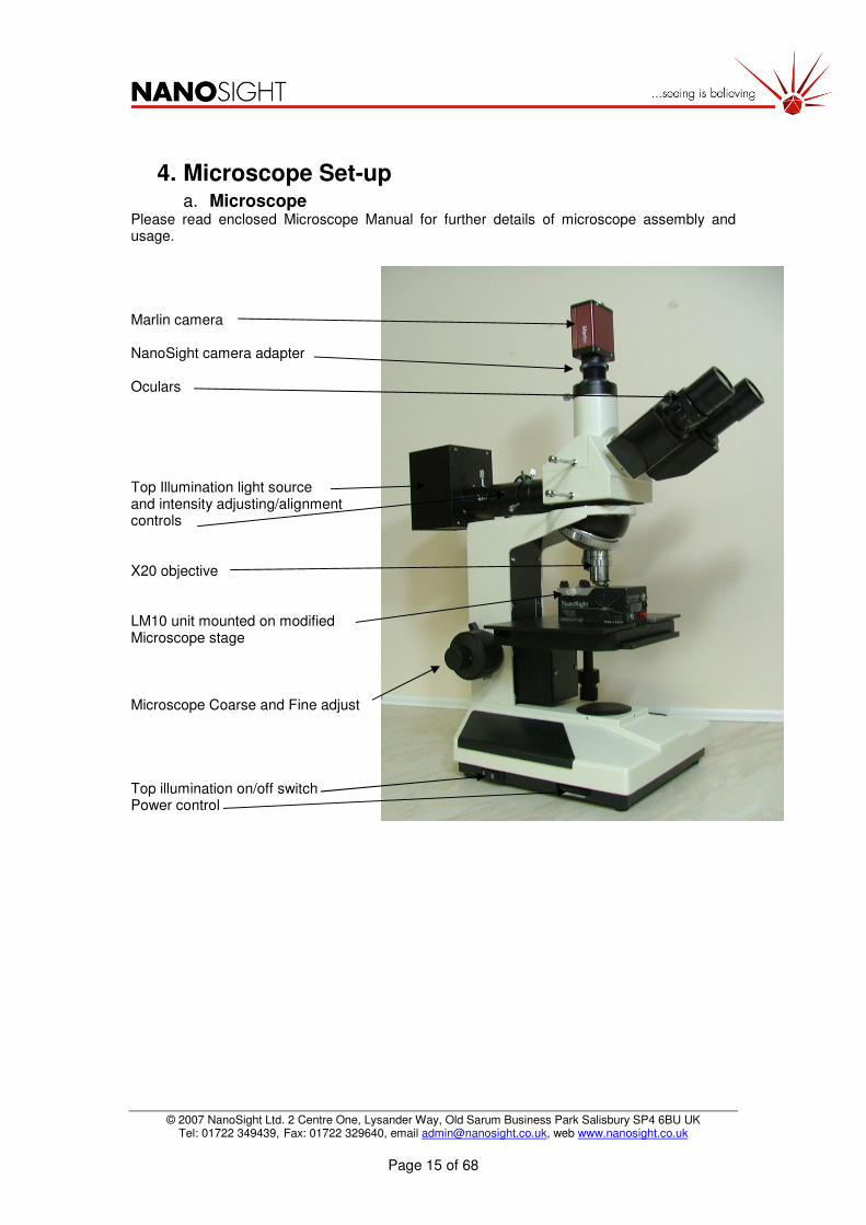
4. Microscope Set-up a. Microscope
Please read enclosed Microscope Manual for further details of microscope assembly and usage. Marlin camera NanoSight camera adapter Oculars Top Illumination light source and intensity adjusting/alignment controls X20 objective LM10 unit mounted on modified Microscope stage Microscope Coarse and Fine adjust Top illumination on/off switch Power control
© 2007 NanoSight Ltd. 2 Centre One, Lysander Way, Old Sarum Business Park Salisbury SP4 6BU UK Tel: 01722 349439, Fax: 01722 329640, email [email protected], web www.nanosight.co.uk
Page 16 of 68
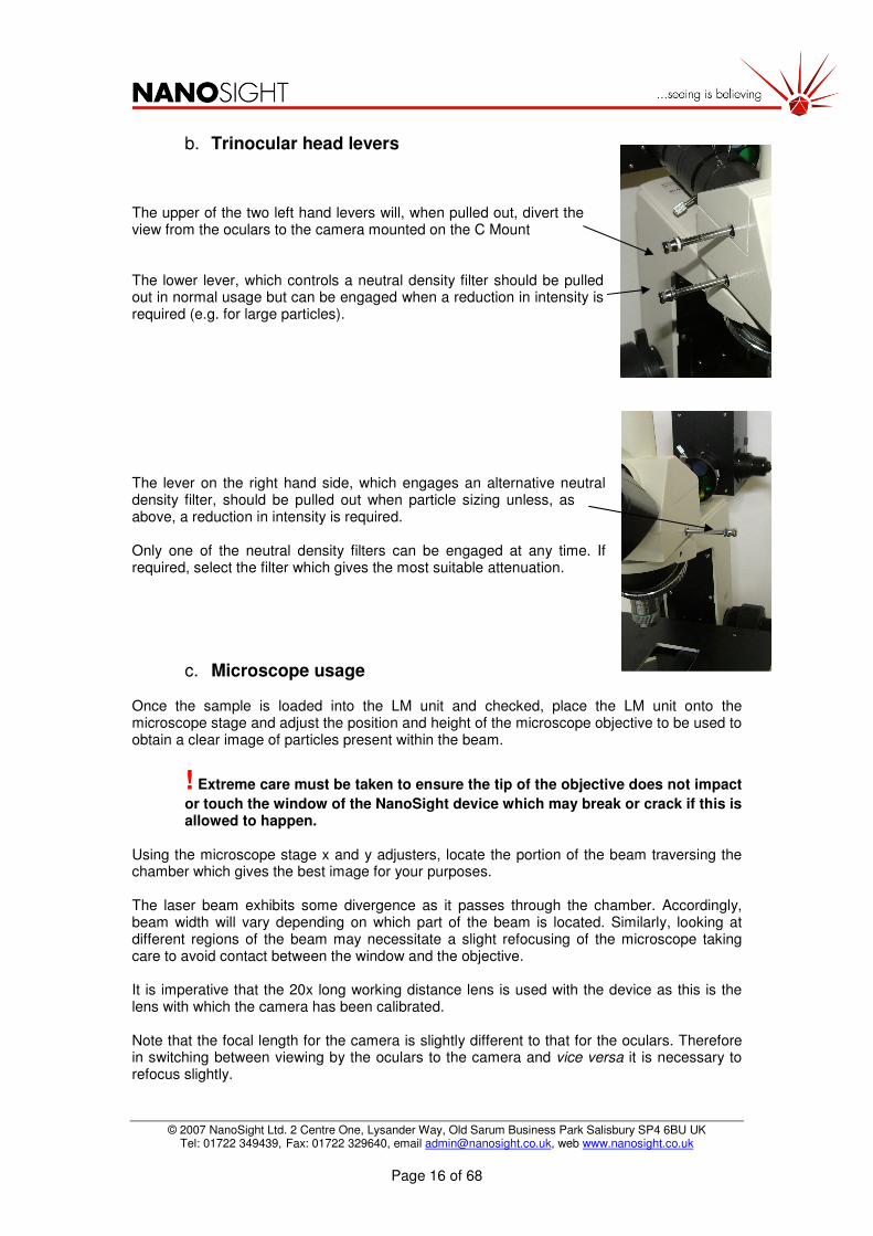
b. Trinocular head levers The upper of the two left hand levers will, when pulled out, divert the view from the oculars to the camera mounted on the C Mount The lower lever, which controls a neutral density filter should be pulled out in normal usage but can be engaged when a reduction in intensity is required (e.g. for large particles). The lever on the right hand side, which engages an alternative neutral density filter, should be pulled out when particle sizing unless, as above, a reduction in intensity is required. Only one of the neutral density filters can be engaged at any time. If required, select the filter which gives the most suitable attenuation.
c. Microscope usage Once the sample is loaded into the LM unit and checked, place the LM unit onto the microscope stage and adjust the position and height of the microscope objective to be used to obtain a clear image of particles present within the beam.
! Extreme care must be taken to ensure the tip of the objective does not impact
or touch the window of the NanoSight device which may break or crack if this is allowed to happen.
Using the microscope stage x and y adjusters, locate the portion of the beam traversing the chamber which gives the best image for your purposes. The laser beam exhibits some divergence as it passes through the chamber. Accordingly, beam width will vary depending on which part of the beam is located. Similarly, looking at different regions of the beam may necessitate a slight refocusing of the microscope taking care to avoid contact between the window and the objective. It is imperative that the 20x long working distance lens is used with the device as this is the lens with which the camera has been calibrated. Note that the focal length for the camera is slightly different to that for the oculars. Therefore in switching between viewing by the oculars to the camera and vice versa it is necessary to refocus slightly.

© 2007 NanoSight Ltd. 2 Centre One, Lysander Way, Old Sarum Business Park Salisbury SP4 6BU UK Tel: 01722 349439, Fax: 01722 329640, email [email protected], web www.nanosight.co.uk
Page 17 of 68
5. LM10 Usage a. Assembling the LM Sample Unit
The LM sample unit can be assembled as follows:
1) Switch off unit and remove power lead. 2) Clean all necessary parts (see below). 3) Lay cleaned glass element into unit. 4) Ensure the ‘O’-ring is bedded correctly in its channel in the top plate of the device. 5) Lay top plate on glass element and adjust gently until plate locates. 6) Drop in four screws and finger tighten loosely alternately in opposite diagonal pairs.
The LM10 unit is now ready to inject a sample.
b. Injection into the LM Unit Load the sample into the sample chamber using a syringe (without needle). The Luer fittings are designed to accept standard syringe bodies of all sizes. Note that high pressures can inadvertently be generated when narrow bore (e.g. 1-2 ml) syringe bodies are used. To avoid generating pressures which might result in the sample bypassing the seals in the sample chamber or damaging the window, care must be taken to introduce the sample slowly.
Similarly, care should be taken to avoid the introduction of bubbles at this stage. The LM sample unit should be tilted such that the syringe is injecting vertically upwards, allowing the chamber is filled slowly against gravity.
The LM laser module has an aperture positioned in the recess where the optical flat sits to allow the laser beam to exit. Therefore it is critical that liquid does not leak under the ‘o’ ring and down this hole as it could cause irreparable damage to the laser inside. The chamber should only hold 0.5ml of liquid; therefore if you have injected this volume and have not filled the chamber, there is a leak. In this case you should remove the sample with the syringe, remove the top plate and flat and look for evidence of liquid outside of the sample chamber. This can be an indication of one of the following:
a) The sample was injected too rapidly. b) The ‘o’ ring was not seated suitably. c) The top plate was not screwed down sufficiently. d) The wrong ‘o’ ring for the solvent being injected was used (see ‘o’ ring solvent
selection guide at end of manual). e) The flat is physically damaged, meaning the ‘o’ ring cannot seal properly. f) The solvent is so thin that sealing is very hard – extra cleaning and slightly more
torque may be needed when tightening screws than normal. So long as a vast excess of liquid has not been injected it is unlikely to cause any damage and simply drying all surface (including the aperture) should bring the unit back to normal operation.
! Occasionally a bubble may be present in the chamber and in the path of the laser beam. This might cause some degree of specular reflection of the laser beam off the bubble surface. The bubble must be removed before viewing through the microscope. A properly prepared and loaded sample will appear as a clear sample through which the laser beam can be seen as a thin line passing through the sample chamber. If the beam appears very bright and appears to ‘bloom’ within the sample, the sample is too concentrated and must be further diluted before viewing via the microscope.

© 2007 NanoSight Ltd. 2 Centre One, Lysander Way, Old Sarum Business Park Salisbury SP4 6BU UK Tel: 01722 349439, Fax: 01722 329640, email [email protected], web www.nanosight.co.uk
Page 18 of 68
c. Adjusting the Microscope
Once the sample is loaded and checked as above, place the LM unit onto the microscope stage and adjust the position and height of the microscope objective to be used to obtain a clear image of particles present within the beam. ! Extreme care must be taken to ensure the tip of the objective does not impact or touch the window of the NanoSight device which may break or crack if this is allowed to happen. Using the microscope stage x and y adjusters, locate the portion of the beam traversing the chamber which gives the best image for your purposes. The laser beam exhibits some divergence as it passes through the chamber. Accordingly, beam width will vary depending on which part of the beam is located. Similarly, looking at different regions of the beam may necessitate a slight refocusing of the microscope taking care to avoid contact between the window and the objective. It is imperative that the 20x long working distance lens is used with the device as this is the lens with which the camera has been calibrated. Please contact NanoSight to discuss if necessary. Note that the focal length for the camera is slightly different to that for the oculars. Therefore in switching between viewing by the oculars to the camera and vice versa it is necessary to refocus slightly.
d. View or Capture Images Once an image can be seen either by viewing via the oculars or by the camera, a movie can be recorded using suitable camera settings as discussed in Section 3 below.
e. Loading a New Sample To remove a sample, simply extract using a syringe. The chamber can be rinsed/cleaned by flushing through the chamber using fresh particle-free water or solvent prior to loading with a different sample. In this instance it is recommended that a tissue be held lightly at the output port to soak up the excess solvent from flushing. Between samples which differ significantly in terms of solvent, particle type or particle loading, it is advisable to dissemble the top plate and rinse and dry thoroughly the optical element and top plate as described below.
f. Cleaning Depending on sample type and length of use, it may prove necessary to clean the chamber and optical surface of the LM sample unit.
Flare spot where laser beam emerges
Particles seen most clearly here
Window

© 2007 NanoSight Ltd. 2 Centre One, Lysander Way, Old Sarum Business Park Salisbury SP4 6BU UK Tel: 01722 349439, Fax: 01722 329640, email [email protected], web www.nanosight.co.uk
Page 19 of 68
! Before cleaning the system, the laser MUST be switched off and the power disconnected. Failure to take these precautionary steps may expose the user to direct Class 3B radiation. Once the power has been disconnected, the unit may be cleaned as follows:
1. Empty the sample chamber by extracting all residual fluid by syringe via the Luer ports.
2. Unscrew the nuts securing the top plate (housing the viewing window) and lift off the top plate.
3. Clean the inside of the window by gently wiping it with a tissue wet with either ethanol, acetone or other solvent required to remove all traces of the sample being analysed.
4. Rinse with deionised water.
5. Dry surfaces of the window with optical grade lens cleaning tissue.
6. An air stream (e.g. from a can of compressed air) should be used to blow any residual liquid from the input and output channels (luer ports) through which the sample is introduced into the chamber. Redry the surfaces with a tissue if necessary.
7. Carefully remove the glass optical flat seated in the upper surface of the main device housing. This can usually be achieved by inverting the unit so the optical flat drops out (ensuring it is caught on a soft surface from a small height e.g. onto hand). Never use a sharp instrument to prise the flat out of its seating or irreparable damage may occur.
8. Carefully wipe all surfaces of the optical flat taking special care with the upper surface of the optical element onto which the top plate is located and the bevelled edge through which the laser beam is launched into the system. This can be done as before with a lens tissue or cotton bud damped with solvent.
9. When all optical surfaces have been cleaned and are dry, reassemble (taking care to ensure the Viton gasket (‘O’-ring) on the underside of the top plate is correctly located in its channel), using only finger-tight pressure to clamp down the top plate using the metal screws and tighten with the tool on the LM unit power supply.
10. DO NOT OVERTIGHTEN.
! Under no circumstances must liquid be allowed to enter the housing of the LM unit at any time. This will cause irreparable damage to the laser mounted within the unit. Take care not to abrade or scratch the optical flat surface, or introduce particulates or contaminants onto the surface. If necessary, other cleaning agents may be employed such as dilute mild detergents, or even dilute acid washes prior to a final solvent cleaning step. The NanoSight device is normally supplied with NanoSorb B optical flats which are relatively robust. However, treat all optical surfaces with the same care as would be employed with equivalent surfaces on your microscope. The optical flats are an integral part of the instrument and may need replacing if scratched or damaged. Replacement NanoSorb B optical flats can be supplied by NanoSight (pricing on request). If in doubt about the choice of solvent and its compatibility with any part of the NanoSight device, please contact us for further information.
g. Storage Between uses of the NanoSight LM unit, or for longer term storage, the unit must be cleaned as described above and stored with no fluids in the chamber.

© 2007 NanoSight Ltd. 2 Centre One, Lysander Way, Old Sarum Business Park Salisbury SP4 6BU UK Tel: 01722 349439, Fax: 01722 329640, email [email protected], web www.nanosight.co.uk
Page 20 of 68
6. NTA Software Usage a. Aim
The aim of this Section is to take the user step-by-step through the NTA (Nanoparticle-Tracking Analysis) software from image capture to the production of a particle size distribution chart. The system allows for a degree of user interaction in the analysis and hence this document will allow the user to make appropriate decisions and gain consistent results. See section 5 for description of how to locate the correct position to view the particles.
b. System Requirements The software is designed for optimal use with a system operating on Windows XP Professional. It is recommended that the system used to run the software should have at least 1GB of RAM, 80GB of free hard disc space (for video storage) and the equivalent of a 3GHz Pentium processor or higher. It is not possible to test the software with the full range of computers on the market. Therefore NanoSight strongly recommends the use of the PC that they specify directly and is included with your order. The software requires a blue security dongle which should be inserted into the USB port on the computer and installed prior to using the software. Information regarding installation of the software and the dongle can be found in the installation document.
c. Start-Up The software comes preinstalled on NanoSight supplied computers and can be loaded either from the desktop (NTA 1.5) or from the start menu (under All Programs � NanoSight� NTA1.5).
d. Image Capture This function can be initiated using the ‘Capture’ button on the main interface.
Figure 1: Video capture interface.

© 2007 NanoSight Ltd. 2 Centre One, Lysander Way, Old Sarum Business Park Salisbury SP4 6BU UK Tel: 01722 349439, Fax: 01722 329640, email [email protected], web www.nanosight.co.uk
Page 21 of 68
Step 1: Auto Settings: When switched on this feature allows the software to select appropriate shutter and gain settings (based on the brightness of the particle present) for the sample being interrogated. This feature should be used only for mono-dispersed samples. The green lines on the shutter and gain sliders indicate current best setting. Text below the Stop button show the detection threshold that is currently being used, the number of particles identified and trackable (red crosses on the image) and the total number of centres found (including the centres that are rejected, indicated by blue crosses). For poly-dispersed samples this feature should be turned off and the user should select appropriate camera settings (see steps 2,3+4). Step 2: Shutter – Determines the length of time the shutter is open for and therefore how much light is captured from the particles. Dim particles (associated with small particles or particles with a low refractive index) need to be captured with a longer shutter opening time. To avoid over exposure, bright particles (larger or high refractive index particles) should be captured with a shorter exposure time. Whilst the shutter is open, the particles will move and hence produce a degree of image smudging or blurring. This may adversely affect the centering of the particles and hence the estimated particle distribution profile. Therefore, to increase the accuracy of the system, the images should be captured using the lowest shutter speed compatible with visualising the particles. In practice a shutter of less than 1000 should be used. The software will not allow the user to select a shutter value of more than 1500 (shutter bar will turn red) as this shutter duration causes the camera to reduce its frame rate i.e. the shutter duration is longer than frame duration. Figure 2 below shows the order in which you should reduce the shutter and gain.
Figure 2: Schematic showing order of changes to shutter and gain,����indicates decrease parameter if too bright.
Step 3: Gain – Acts to multiply the intensity reading from each pixel in the array. The gain should generally be set high to allow the shutter to be reduced to a minimum in order to reduce particle blurring. Step 4: Brightness – The camera used to capture the image has a dynamic range of 256 gray scale increments. Altering the brightness shifts the intensity of this 256 greyscale range. Setting the brightness so as to detect very dim particles, may result in bright particles in the same image having an intensity which may exceed the maximum of the 256 greyscale (saturation). By varying the brightness of the 256 greyscale values to allow for bright particles, dim particles may now be below the detection threshold of the system. Generally the brightness should be left as zero (the default value). The brightness, gain and shutter should be used in combination to produce an optimal image for the analysis suite. Particle centering is performed by finding the centroid of the intensity profile for each particle. If all of the pixels within the footprint for a particular particle are over-exposed, then the software has no intensity profile from which it can find the particle centre and a simple geometric centering is performed. Therefore to achieve accurate particle sizing, the camera settings should be manipulated to produce images which have an intensity profile with few/none of the pixels saturated. Also, as mentioned previously, the shutter should be kept to a minimum to avoid particle blurring during the exposure period.
Shutter 4000 Gain 680
Shutter �300 Gain 680
Shutter �0 Gain 0
Shutter 300 Gain �0

© 2007 NanoSight Ltd. 2 Centre One, Lysander Way, Old Sarum Business Park Salisbury SP4 6BU UK Tel: 01722 349439, Fax: 01722 329640, email [email protected], web www.nanosight.co.uk
Page 22 of 68
Figure 3: Example of an optimal image to allow accurate particle centering.
Figure 4: Example of poor image for analysis suite.
Figures 3 + 4 show the same sample but captured under different capture settings. As can be seen from Figure 4, the particles appear as over-exposed bright white discs. Each pixel within the footprint of the particle will have a saturated intensity of 255, and hence it is very difficult to centre the particle. In addition, the camera settings are such that the image suffers from increased background noise. By decreasing the shutter and the gain the diffraction patterns from the periphery of the particles can be reduced as well as reducing the over exposed particles. Step 5: Alternate Gamma – This function alters the relationship between the intensity recorded on the camera CCD array and that which is displayed by the computer monitor. Without gamma correction the relationship is that of straight line graph (linear). With the correction switched on, the camera preferentially amplifies the signal from the dim pixels whilst maintaining a straight line relationship for brighter pixels. This allows both small and

© 2007 NanoSight Ltd. 2 Centre One, Lysander Way, Old Sarum Business Park Salisbury SP4 6BU UK Tel: 01722 349439, Fax: 01722 329640, email [email protected], web www.nanosight.co.uk
Page 23 of 68
larger particles to be visualised in the same image without the brighter particles dominating the image. Use this option when very small particles are present and with polydisperse systems. Step 6: Set Capture Duration – This determines the length of video which is captured. Longer videos allow more accurate particle distributions to be produced. Adequate capture duration is largely dependent on the size of the particles present in the sample and their concentration. Small particles have a more exaggerated Brownian motion, hence the rate of particle refreshment is increased and sufficient numbers of particles can be included in the particle size distribution. The minimum time for capture for a relatively high concentration of monodisperse, small (<200nm) particles is 30 seconds. With low concentrations of larger particles, longer capture durations (e.g.166 seconds) should be used to allow a sufficient number of particles to be included in the particle size distribution. The camera operates at 30 frames per second (fps); therefore a 20 sec clip comprises 600 frames. Step 7: Record – Starts the video capture. The video can be stopped at any time by using the ‘Stop’ button. Figure 1 shows the camera capture interface. As can be seen at the top of the image, the software informs the user if any frames are dropped from the camera upon capture. Dropped frames are usually associated with a slow processor speed, hard discs which are nearly full, or with high computer activity. It is important to record a video clip with no dropped frames as this will affect the calculated particle sizes. If the computer drops (skips) frames whilst the video is capturing, the preview screen can be switched off in order to help reduce the computer workload. This option is located in the ‘Camera’ section of the toolbar under ‘Display Video During Capture.’ There is also a buffer to help preserve data integrity, here ‘file lag’ written next to the skips should for the majority of the time be less than 10 and greater than 500 may indicate a problem. At the end of the video capture the user is prompted to choose the destination where the file is saved. Step 8: Temperature Display - For LM20 systems the instrument will automatically feed the temperature of the laser unit into the software and record this for the analysis phase, the temperature will be displayed in the lower left hand region of the capture screen. Step 9: Temperature Control – For LM20 systems sold with a temperature control top plate the temperature of the unit can be controlled from the video capture page. This feature can be found at the bottom right of the camera control settings. By increasing the value displayed, the temperature control unit will actively increase or decrease the temperature of the unit to match the selected value.
© 2007 NanoSight Ltd. 2 Centre One, Lysander Way, Old Sarum Business Park Salisbury SP4 6BU UK Tel: 01722 349439, Fax: 01722 329640, email [email protected], web www.nanosight.co.uk
Page 24 of 68
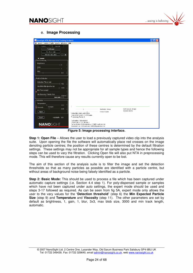
e. Image Processing
Figure 5: Image processing interface.
Step 1: Open File – Allows the user to load a previously captured video clip into the analysis suite. Upon opening the file the software will automatically place red crosses on the image denoting particle centres; the position of these centres is determined by the default filtration settings. These settings may not be appropriate for all sample types and hence the following steps can be used to vary the filtration. Clicking Open file will also put NTA in preprocessing mode. This will therefore cause any results currently open to be lost. The aim of this section of the analysis suite is to filter the image and set the detection thresholds so that as many particles as possible are identified with a particle centre, but without areas of background noise being falsely identified as a particle. Step 2: Basic Mode: This should be used to process a file which has been captured under automatic capture settings (i.e. Section 4.4 step 1). For poly-dispersed sample or samples which have not been captured under auto settings, the expert mode should be used and steps 3-17 followed as required. As can be seen from fig 5A, expert mode only allows the user to the vary values for the ‘Detection threshold’ (step 6) the Min Expected Particle Size (step 9) and Temperature and Viscosity (step 11). The other parameters are set by default as brightness, 1, gain, 1, blur, 3x3, max blob size, 3000 and min track length, automatic.

© 2007 NanoSight Ltd. 2 Centre One, Lysander Way, Old Sarum Business Park Salisbury SP4 6BU UK Tel: 01722 349439, Fax: 01722 329640, email [email protected], web www.nanosight.co.uk
Page 25 of 68
Figure 5A. Processing interface with Basic Mode enabled.
The aim of steps 3 – 7 is to set image filtration settings to cause the software to place a red cross in the centre of the particles on the screen that the user can distinguish as particles without highlighting any areas of background noise. The worked examples (section 4.8) will help contextualise the parameters explained in the following paragraphs. Step 3: Gain – Again, the same function as in the camera capture section. The gain can be used to multiply the intensity value for each pixel, bringing dim particles above the minimum value that the software accepts as a particle (see Detection threshold – Step 5). High gain values will also increase background noise to a level at which it may also be falsely deemed a particle. Generally, gain and brightness are used antagonistically. Gain can be used to increase the numerical difference between the particle intensity and that of the noise. The brightness can now be used to drop the intensity of the background noise below the detection threshold. Step 4: Brightness – This varies the captured image brightness. It should be increased to remove background scatter (i.e. scatter not directly from particles). Step 5: Blur – The blur function allows the user to smooth the intensity profile for each particle. This allows accurate centering of the particles and also for the user to remove false centres from the analysis. Particles may appear to have a ring structure around the particle (due to diffraction). These may have false centres located on them. Blurring can be used to merge the rings into the main region of the particle and hence create a footprint with one centre and no false centres. Blurring can also aide removal of false centres located in regions of noise. Note, that ‘false’ centres are frequently very transitory and short lived. As such no such centre is likely to survive for more than a low number of frames and therefore is unlikely to be included in the analysis given an adequate ‘minimum track length’ setting described below. Minimum of 3x3 is recommended and normally 5x5 is suitable. Step 6: Detection Threshold: This value determines the minimum intensity required for an area of light intensity to be determined as a particle. In practice, the user should aim to adjust this setting such that all clearly recognisable particles have been centred with a red cross and there are few, if any, false centres marked by red crosses where there are no clearly recognisable particles. Step 7: Maximum Blob Size – This determines the maximum size (in terms of number of pixels) of a particle for it to be deemed a particle. This feature can be used to remove bright

© 2007 NanoSight Ltd. 2 Centre One, Lysander Way, Old Sarum Business Park Salisbury SP4 6BU UK Tel: 01722 349439, Fax: 01722 329640, email [email protected], web www.nanosight.co.uk
Page 26 of 68
particles from an analysis. Large, high refractive index particles will scatter large amounts of light and hence will appear to have a larger footprint than a dimmer particle. In a mono-dispersed sample this feature can be used to discount contaminant particles. Alternatively this feature can be used in a poly-dispersed sample to discount the larger population of particles. This allows a two-step approach of sample analysis allowing accurate, independent measurement of two particle populations within the same video clip. Step 8 Minimum Track Length - This is the minimum number of frames a particle must be tracked for to be accepted as a valid particle. Brownian motion is a random process whereby a particle may move a large or small distance over a certain time period (e.g. within the 33msec between frames). On average however, a particle of a specific size will move a fixed and reproducible distance if enough individual movements are averaged. Therefore the minimum lifetime can be used to ensure enough particle steps are taken for an adequately accurate average of the particle movement to be produced. Increasing this value will increase the confidence in the results, but will decrease the number of particles analysed. Larger particles can be analysed using a longer minimum lifetime than smaller particles because larger particles have a more limited Brownian motion than smaller particles and will remain in the detection volume for longer. As particle movement becomes more restricted the accuracy with which the size can be determined by Brownian motion is reduced; this can be offset by only allowing particles in the analysis which the software has tracked for extended periods of time. Smaller particles should be analysed using a shorter minimum lifetime as these particles may only exist within the field of view for short periods of time, due to their increased speed of Brownian motion and correspondingly greater distances travelled. By clicking the check box as shown in the diagram below this function is automated by the software and removes the need to select different minimum track lengths for different sized particles. By checking this box, the software automatically relates the calculated to particle size, to the length of time the particle should have been tracked for to get an accurate average of particle size. Hence within the same video clip, particles which are sized at 100nm will need to be tracked for 15 frames whilst particles which are sized at 400nm will need to be tracked for 60 frames. The length of time the particles are tracked for is calculated by the software on a particle by particle basis and the length of time is related to a confidence level in the particle size estimation for differently sized particles. The value selected for the minimum track length is also related the viscosity of the solvent selected. Hence a 100nm particle in water (viscosity of 1 cp) will only be required to be tracked for 15 frames whilst a 100nm particle suspended in a solvent of 2cp will be required to be tracked for 15x2 = 30 frames.
Step 9 Minimum Expected Particle Size: The value the user selects here determines the maximum distance (pixels) from its position in frame 1 that the software will look for a particle in frame 2. It also establishes an exclusion zone around a particle. If another particle enters this exclusion zone then the software excludes the information from both particles. This prevents the software erroneously joining the tracks from two different particles. By setting this value too large, larger exclusion zones are created around a particle and a lot of valid information is lost through a reduction in number of tracks analysed. By setting it too small, the particle may jump out of the zone and its movement will not be picked up by the software. In order to accurately determine the maximum distance a particle jumps in the sample, the ‘Max Jump Toggle’ button should be used. This feature zooms in on a point where a particle can be seen by left clicking with the mouse on the particle; the software toggles between two successive frames (see Fig 5.1 + 5.2). This allows the user to estimate

© 2007 NanoSight Ltd. 2 Centre One, Lysander Way, Old Sarum Business Park Salisbury SP4 6BU UK Tel: 01722 349439, Fax: 01722 329640, email [email protected], web www.nanosight.co.uk
Page 27 of 68
the distance each particle jumps (in pixels); the crosshair can be used as an aide to estimate the jump distance in pixels. The size of the crosshair alters as the user changes the ‘Min Expected Particle Size’ slider. The user should sequentially zoom in on several particles to estimate the maximum distance jumped by the particles and 1 or 2 extra pixels should be added to the value to allow a margin for particles which may uncharacteristically jump slightly larger distances.
Figure 6: Image 1 of a zoomed-in image showing the position of a particle in two successive frames.
Figure 7: Image 2 of a zoomed-in image showing the position of a particle in two successive frames.
Alternatively if the user has prior knowledge of the particle sizes contained within the sample, the above process can be by-passed by simply using the slider bar to select a particle size which correlates to the minimum particle size that is expected in the sample.

© 2007 NanoSight Ltd. 2 Centre One, Lysander Way, Old Sarum Business Park Salisbury SP4 6BU UK Tel: 01722 349439, Fax: 01722 329640, email [email protected], web www.nanosight.co.uk
Page 28 of 68
Step 10 Pre-Process – This button will take the user back to the interface showing the first frame of the video allowing the user to alter the image settings further. Step 11 Temperature and Viscosity – The Brownian motion of a particle is influenced by the temperature and the viscosity of the fluid in which they are suspended. These values therefore need to be input by the user for accurate calculation of the particle sizes. By clicking the tick box next to the temperature slider bar, the temperature and viscosity are linked. If the box is red, the temperature will automatically be linked to the viscosity of water. When the user changes the temperature, the viscosity changes automatically for samples dispersed in water. For samples not dispersed in water, un-tick the box (it will appear white) and enter the viscosity value for the solution at the indicated temperature.
Figure 8: Diagram to show linked values of temperature and viscosity for water.
Step 12 Bin width adjustment and X Axis Scaling and off-setting– These two slider bars allow the user to determine the plotting parameters of the particle distribution graph. The bin width allows the user to vary the size of the histogram bin in nm. The X Axis slider allows the user to vary the maximum particle size in nm of the particle distribution. The X axis can also be ‘picked up’ (by clicking on it with the mouse) and shifted or offset from side to side. Step 13 Process Sequence – Starts the analysis. The analysis can be paused, restarted and stopped at any point. When paused, the analysis can be incremented one frame at a time by pressing the forward arrow on the keyboard. This can be useful for following the analysis of any given particle in more detail. Note, however, the analysis cannot be run backwards using the back arrow. Step 14 Select Start/Stop position of video. Below the image there is a time line. Clicking on this with the left mouse button will change the image of the video that is displayed. Clicking with the right mouse button will move the green/red line indicating the start/stop position that the analysis will analyse. To toggle between the start/stop selection click the left mouse button on the timeline. Step 15 Excluding An Area From The Analysis: During video capture, unwanted light scattered from a static object, such as dirt on the optical flat or chamber window, may be included in an analysis. The field of view can be modified to exclude these static or very slow moving regions of scatter by clicking using the mouse on the field of view and dragging an exclude box over the region to be excluded. Multiple areas can excluded. By right-clicking on the mouse all the exclusion areas are removed from the analysis.

© 2007 NanoSight Ltd. 2 Centre One, Lysander Way, Old Sarum Business Park Salisbury SP4 6BU UK Tel: 01722 349439, Fax: 01722 329640, email [email protected], web www.nanosight.co.uk
Page 29 of 68
Figure 9: Diagram to show how the field of view can be restricted to remove areas of static scatter.
Step 16 Background Extraction: This function can be used to remove constant background noise from the analysis. Some solvents such as toluene scatter light even when there are no particles present in the sample chamber. The light scattered from the toluene can be removed using the background subtraction so that only light scattered form the particles is included in the analysis. This feature can be found in the ‘Advanced’ drop-down menu. Step 17 Varying the Experimental Parameters during analysis– During the analysis the Bin width and X axis value can be altered at any point without affecting the final analysis. All other filtration values can be altered as the analysis proceeds but the changes will only effect the remaining frames i.e. changing the viscosity half way through the analysis will not influence the calculated values in the first half of the analysis. By pressing the ‘Replot’ button at the end of the analysis, mid-analysis changes in Temperature and Viscosity can be recalculated over all frames. Changes in Brightness, Gain, Blur, Detection Threshold, Max Blob Size, Max Particle Jump cannot be corrected for using the ‘Replot’ function. Whilst these values can be changed mid-analysis, their effects are only seen in subsequent frames. If necessary the analysis should be restarted using the new parameters. Step 18 Drift Correction Drift is generally associated with heating of the fluid and resulting convection currents; it manifests as a tendency for all the particles to move with a common vector. There are two components to the drift indicator. The WHITE box indicates the instantaneous drift measured in any specific frame whilst the RED box indicates the overall drift averaged out over all the frames analysed to that point.
Figure 10: Enlarged image of drift correction.
Drift within a system will result in the particles appearing to be smaller than they actually are. Drift correction can be automatically removed by clicking the ‘Auto Drift correction’ in the ‘Advanced’ drop down menu on the tool bar. The drift correction will remove any over propensity for the particles to move in a specific vector and will recalculate particle sizes taking into account its removal.

© 2007 NanoSight Ltd. 2 Centre One, Lysander Way, Old Sarum Business Park Salisbury SP4 6BU UK Tel: 01722 349439, Fax: 01722 329640, email [email protected], web www.nanosight.co.uk
Page 30 of 68
Step 19: Changing the Display By clicking on the buttons in the bottom-right corner of the interface (zoomed in above, Figure 11) the user can alter the image displayed on the software. The software defaults with the particle distribution overlaid on the captured image.
Figure 11: Enlarged image to show how user can change display from video clip to particle distribution.
Clicking the left button will display the video of the particles only (Figure 12 (a)). Clicking on the right screen will bring up the particle distribution again (Figure 12 (b)) and then clicking on the right screen for a second time will bring up the particle distribution only (Figure 13) . (a) (b)
Figure 12: (a) Video only (b) Video and data graph.
Figure 13: Data graph only.

© 2007 NanoSight Ltd. 2 Centre One, Lysander Way, Old Sarum Business Park Salisbury SP4 6BU UK Tel: 01722 349439, Fax: 01722 329640, email [email protected], web www.nanosight.co.uk
Page 31 of 68
Figure 14: Typical particle distribution produced by the software.
As can be seen the software will automatically build the particle distribution over the video clip as the analysis proceeds. The software draws the path the particle has taken during its lifetime and calculates the average step jump distance it has taken along this path, from this average the hydrodynamic radius of each particle within the field of view is calculated. As can be seen in Error! Reference source not found., the software produces a mode value for the distribution (in this example 104nm), the user can click on any point in the graph to produce a user line for comparison to the modal value. Each particle is labelled with two numbers (see Error! Reference source not found.4). The top number represents the calculated particle size at that instant and the bottom number represents the number of frames the particle has been tracked for and on which the instantaneous size estimation is based. These values can be switched on and off at any point through the ‘Display’ section of the toolbar.
Figure 15: Particle labels.
f. Batch Capture and Process

© 2007 NanoSight Ltd. 2 Centre One, Lysander Way, Old Sarum Business Park Salisbury SP4 6BU UK Tel: 01722 349439, Fax: 01722 329640, email [email protected], web www.nanosight.co.uk
Page 32 of 68
The software can be configured so that it will automatically capture and analyse a sequence of video clips. This feature may be important when the user wishes to characterise an aggregation or dissolution process.
Batch Capture The batch capture facility can be found under the ‘Advanced’ section of the toolbar. The image on the following page shows the interface used to set the batch capture process:
Figure 15: Interface used to control the batch capture process.
The duration of video capture can be determined (Duration of each Sequence), the time between the start of each capture (Frequency of Capture) and the number of cycles to be captured (Number of Captured Sequences). For each cycle the video is captured at the start of the cycle and then written to disc. For long video clips i.e. 60 seconds, the software can take 60 seconds to write the information to disc. Hence for a 60 second video clip the frequency of capture should not be set to less than 120 seconds to avoid the computer trying to capture video whilst writing the previous information to disc. In such cases many frames would likely be dropped as the computer struggles to keep up with the demand. The sequence captured can be processed using common software filtration parameters. The sequence can be loaded using the interface as is shown below i.e. found under the ‘Advanced’ toolbar.
Batch Process Any sequence of files captured, either as part of a batch capture run (as described in the section above) or individually, can be processed using common software processing parameters. The sequence can be loaded using the interface as is shown below i.e. found under the ‘Advanced’ toolbar. Either locate and load the separate files individually or click the ‘Find Sequence’ button and locate the first movie of a batch. This will load in all files in the sequence for analysis. When the user clicks ‘go’ the movies will be processed in sequences using the parameters that are stored in the process text file (see export files, below) for the first movie. Therefore it is necessary to analyse the first movie by the normal method in order to set the parameters that should be used for the rest of the analyses.

© 2007 NanoSight Ltd. 2 Centre One, Lysander Way, Old Sarum Business Park Salisbury SP4 6BU UK Tel: 01722 349439, Fax: 01722 329640, email [email protected], web www.nanosight.co.uk
Page 33 of 68
Figure 16: Interface to load video clips into the Batch Process facility.
Figure 17: Typical image produced from batch capture process.
As can be seen from Figure 17 the software will automatically overlay distributions produced from the batch capture process. Each line can be added or removed by clicking on the coloured button for that line. To view which line represents which graph it is possible to right click on the coloured button, the file name of that coloured line will then be displayed near the top of the screen.

© 2007 NanoSight Ltd. 2 Centre One, Lysander Way, Old Sarum Business Park Salisbury SP4 6BU UK Tel: 01722 349439, Fax: 01722 329640, email [email protected], web www.nanosight.co.uk
Page 34 of 68
g. Output Parameters
Screen display Some of the most important parameters are displayed on the screen. These are outlined below:
Modal size The modal size of the particle is displayed in the blue line along the top of the screen.
User lines
To identify secondary peaks or to measure concentration between two lines (see below) two user lines are available to the user. These can be accessed by clicking the left/right mouse button on the bar graph display. The x-axis value at which the user line is positioned is displayed in the text at the bottom of the screen.
Mean Size
The average of all particle sizes is listed at the bottom of the screen. Concentration
The software will out put an estimation of the particle concentration in the sample based on the number of particles identified and the known volume of the sample interrogated. The information is displayed at the bottom of the interface as is shown below showing the average number of particles seen per frame and the corresponding particle concentration. By left clicking on the distribution and then right clicking on a second part of the distribution the user can select a region of the distribution over which the software will calculate a concentration. This allows the user to break up the size distribution and determine the concentration of specific sub-populations within the distribution. The concentration of the selected area is also displayed below.
Graphical Output Scales The particle sizing data output can be displayed as either a number plot or a concentration plot (under the ‘Graph’ section of the toolbar). For a number plot, the graph plots the particle size against the number count of particles tracked. However, since smaller particles move faster under Brownian motion, they will diffuse in and out of the field of view faster than larger particles, leading to more small particles being counted and over-estimating the number of small particles present compared to larger ones. The concentration plot weights the data to ensure that a true reflection of the size distribution is presented based on the concentration of particles of different sizes (this is the default setting). Other options that are available are:
Surface area and Volume. Here the frequency is simply multiplied by the square/cube of the radius respectively to give relative proportions of surface area or volume contributed by each size range.
Diffusion coefficient Plots the diffusion coefficient of particles instead of size on the x-axis.
Draw Bars Toggles the standard bar-chart.

© 2007 NanoSight Ltd. 2 Centre One, Lysander Way, Old Sarum Business Park Salisbury SP4 6BU UK Tel: 01722 349439, Fax: 01722 329640, email [email protected], web www.nanosight.co.uk
Page 35 of 68
Draw Multigraphs Toggles the lines from batch process.
Log scale Rescales the x-axis on logarithmic scale.
Cumulative Undersize and Oversize
Figure 16: Distribution showing cumulative undersize for analysis.
As can be seen from above the D10, D50 and D90 values can be calculated for the sample by using the cumulative undersize function. This function can be found in the ‘Graphs’ dropdown on the toolbar. The D70 value shown is user settable with the slide scale below. D10 is the diameter (in nanometres) of the particle that is the 10
th percentile; this means the
particle 10 percent along the list of individual results, when ranked from the smallest to largest
Report The software can be used to produce a standardised sample report sheet. This feature is found under the ‘Export’ section of the toolbar. By clicking on ‘Set Report Details’ a report template appears into which the user can fill in the relevant details. The user can select which graphs and images they would like to appear on the report. Four different images can be selected to appear on the report. The user can select which images appear on the report in the ‘Export’ section of the toolbar. By clicking ‘Use current Display as Fig 3 or 4’ the user can select which images will be displayed on the report print out, which can be directly printed from the software. Figures 1 and 2 are automatically set. Figure 2 (top right) is automatically the image of the selected frame. Figure 1 (top left) is concentration graph with cumulative undersize overlayed as shown below in figure 16.

© 2007 NanoSight Ltd. 2 Centre One, Lysander Way, Old Sarum Business Park Salisbury SP4 6BU UK Tel: 01722 349439, Fax: 01722 329640, email [email protected], web www.nanosight.co.uk
Page 36 of 68
Figure 17: Preview of Report Diagrams.
Screenshot A bitmap file can be formed from the screen within the area that the image is normally displayed. This is created by pressing F12 button on the keyboard.
Export Data The data which forms the histogram is automatically exported at the end of the analysis and saved in the same folder in which the video file exists. The data is saved as (.csv) file which is automatically recognised by Microsoft Excel. If the user changes any of the parameters and changes the histogram, the new data can be exported by clicking the export button at the bottom left of the interface. The software will export the new data with a new suffix to distinguish form the original data which is outputted. Summary File The following comma separated values (.csv) file is generated via the Export File facility within the programme and is named “xxxx-001-summary.csv”. It is saved to the same location in which the video file (xxxx.avi) is saved (user-selectable) and has the same name (e.g. xxxx as the video. Note that multiple analyses of the same video will be saved separately with an auto-incrementing number to distinguish the different analyses, e.g. usertest-001-summary.csz, usertest-002-summary.csv, etc.. These files can be loaded to/by Excel for further manipulation.

© 2007 NanoSight Ltd. 2 Centre One, Lysander Way, Old Sarum Business Park Salisbury SP4 6BU UK Tel: 01722 349439, Fax: 01722 329640, email [email protected], web www.nanosight.co.uk
Page 37 of 68
[ResultsSummary]
Operator=
SampleDescription=
Diluent=
Concentration=
PreTreatment=
Comments=
TotalFrames=1800
ProcessedFrames=1799
CompletedTracks=776
OverallDrift=228.489557
X-Drift=55.969406
Y-Drift=-221.528560
Calibration=166
Mode=98
Mean=112
UserLine=0
PercentileUndersize size
1 67
2 72
3 73
4 74
5 76
96 174
97 184
98 191
99 233
100 382
BinCentre Count
5 0
15 0
25 0
35 0
45 0
55 0
65 8
75 38
85 87
95 161 105 151
1975 0
1985 0
1995 0
Total no of frames in video
Number of frames used in analysis
Number of particles sized
Drift automatically compensated for unless option deactivated Fixed
Value (size in nm) of highest bin [weighted by values of adjacent bins]
Sum of particle size values for all particles ÷ number pf particles
Percentile undersize values at 1% resolution
Values at centre of each bin (including zero values) at user selected bin width (in this case, 10nm)
Sample description as entered by the user in the Report page

© 2007 NanoSight Ltd. 2 Centre One, Lysander Way, Old Sarum Business Park Salisbury SP4 6BU UK Tel: 01722 349439, Fax: 01722 329640, email [email protected], web www.nanosight.co.uk
Page 38 of 68
Result file The following comma separated value (.csv) file is generated via the Export File facility within the programme and is named “xxxx-001-result.csv”. It is saved to the same location as the video file (xxxx.avi) is saved (user-selectable) and has the same name (xxxx…) as the video. Note that multiple analyses of the same video will be saved separately with an auto-incrementing number to distinguish the different analyses, e.g. usertest-001-result.csv, usertest-002-result.csv, etc.. These files can be loaded to/by Excel for further manipulation.
Values for each bin containing a non-zero value, i.e. empty bins are not displayed. Note that the raw data stored in this table at a 1nm resolution while the particle size distribution graph displayed on the screen or in the report will depend on the bin width selected by the user.
Size (nm) Count
60 1
63 1
64 1
66 3
67 1
69 1
218 1
223 1
235 1
238 1
256 2
268 1
282 1
303 1
382 1
848 1

© 2007 NanoSight Ltd. 2 Centre One, Lysander Way, Old Sarum Business Park Salisbury SP4 6BU UK Tel: 01722 349439, Fax: 01722 329640, email [email protected], web www.nanosight.co.uk
Page 39 of 68
Analysis File The following comma separated values (.csv) file is generated via the Export File facility within the programme and is named “xxxx-001-analysis.csv”. It is saved to the same location in which the video file (xxxx.avi) is saved (user-selectable) and has the same name as the video. Note that multiple analyses of the same video will be saved separately with an auto-incrementing number to distinguish the different analyses, e.g. usertest-001-analysis.csv, usertest-002-analysis.csv, etc.. These files can be loaded to/by Excel for further manipulation.
Parameters set for processing video (also printed out in report)
[Settings]
Pulldown=3
Gain=4
Blur=2
DetectThresh=39
MaxBlob=250
MinTrackLength=20
MaxParticleJump=10
Temperature=19.0
Viscosity=1.0227
BinWidth=10

© 2007 NanoSight Ltd. 2 Centre One, Lysander Way, Old Sarum Business Park Salisbury SP4 6BU UK Tel: 01722 349439, Fax: 01722 329640, email [email protected], web www.nanosight.co.uk
Page 40 of 68
All-tracks File The following comma separated values (.csv) file is generated via the Export File facility within the programme and is named “xxxx-001-alltracks.csv”. It is saved to the same location in which the video file (xxxx.avi) is saved (user-selectable) and has the same name as the video. Note that multiple analyses of the same video will be saved separately with an auto-incrementing number to distinguish the different analyses, e.g. usertest-001-alltracks.csv, usertest-002-alltracks.csv, etc.. These files can be loaded to/by Excel for further manipulation. Particle ID
Track Step X1 Y1 X2 Y2
Diffusion Co
Particle Size
1 2 100.4584 3.868786 95.32211 3.192722 361.9166 117.0273
1 3 95.32211 3.192722 98.14208 2.710382 361.9166 117.0273
2 2 160.4091 2.396104 164.0134 2.3125 172.6027 232.7189
2 3 164.0134 2.3125 165.9162 2.021739 172.6027 232.7189
4 2 99.38546 16.35463 101.3246 22.68264 517.314 78.79213
4 3 101.3246 22.68264 103.5821 23.76014 517.314 78.79213
7 2 450.9534 100.4378 455.8448 99.74518 453.3191 92.52557
7 3 455.8448 99.74518 458.1433 101.3496 453.3191 92.52557
7 4 458.1433 101.3496 454.4592 101.8439 453.3191 92.52557
7 5 454.4592 101.8439 454.0251 100.6831 453.3191 92.52557
7 6 454.0251 100.6831 454.7009 105.0745 453.3191 92.52557
7 7 454.7009 105.0745 457.2028 104.3766 453.3191 92.52557
7 8 457.2028 104.3766 457.1436 107.8561 453.3191 92.52557
7 9 457.1436 107.8561 456.2762 104.8696 453.3191 92.52557
7 10 456.2762 104.8696 456.6437 103.0476 453.3191 92.52557
7 11 456.6437 103.0476 459.4194 101.2233 453.3191 92.52557
7 12 459.4194 101.2233 458.6222 106.3778 453.3191 92.52557
7 13 458.6222 106.3778 454.9494 109.9508 453.3191 92.52557
7 14 454.9494 109.9508 454.9501 104.5261 453.3191 92.52557
7 15 454.9501 104.5261 451.5 96.5 453.3191 92.52557
7 16 451.5 96.5 452.7451 97.71292 453.3191 92.52557
7 17 452.7451 97.71292 451.9704 95.22328 453.3191 92.52557 The data which forms the basis of the particle distribution can be exported in a ‘.csv’ file which can then be imported into an Excel spreadsheet. This is exported automatically at the end of each process. This function is found at the bottom left of the main screen. The data is exported to a file located in the same folder as the original video clip with the suffix displayed added to the file name.
Identity given to each particle analysed
Consecutive steps taken by particle
Estimated diffusion coefficient at end of track
Estimated particle size at end of track
x and y position at current frame
x and y position at next frame

© 2007 NanoSight Ltd. 2 Centre One, Lysander Way, Old Sarum Business Park Salisbury SP4 6BU UK Tel: 01722 349439, Fax: 01722 329640, email [email protected], web www.nanosight.co.uk
Page 41 of 68
7. Worked Examples
200 nm Reference Latex Spheres
Figure 18.1: Diagram showing the ideal camera settings to capture a video of 200 nm
diameter latex particles. The above diagram shows an ideal image of 200 nm latex reference spheres. Notice the shutter speed is very low, combined with a low gain. The shutter is kept low to avoid particle blurring as explained previously. The gain is kept low in order that the particles retain their grey scale image and thus allowing accurate centering of particles. Note the alternate gamma is not used as this option is generally used for very small particles and poly-dispersed systems. For very accurate reading a 60 second analysis will produce a stable particle distribution. The sample contains an ideal concentration of particles.
• Shutter: 92
• Gain: 20
• Brightness : 1
• Alternate Gamma: No
• Time of Capture: 60-90 Seconds.

© 2007 NanoSight Ltd. 2 Centre One, Lysander Way, Old Sarum Business Park Salisbury SP4 6BU UK Tel: 01722 349439, Fax: 01722 329640, email [email protected], web www.nanosight.co.uk
Page 42 of 68
Figure 19.2: Diagram showing the same sample as in Fig 17.1 but captured under auto
capture settings As the sample is mono-dispersed the software can be used to automatically set the capture parameters.
Figure 20.1: Shows the settings used to analyse 200 nm latex reference particles.

© 2007 NanoSight Ltd. 2 Centre One, Lysander Way, Old Sarum Business Park Salisbury SP4 6BU UK Tel: 01722 349439, Fax: 01722 329640, email [email protected], web www.nanosight.co.uk
Page 43 of 68
The below settings shows the ideal values to analyse the 200 nm latex particles. The aim of the parameters are to allow the user to indentify known particles with red crosses. In reality the software is relatively robust to changes in these values and the user should not spend too long on trying to get every particle with a red cross in its centre.
• Brightness: -3 to remove any background noise.
• Gain: 3 makes the dimmest particles visible.
• Blur: 5x5 removes any false centres located between 2 particles which are close together or on the diffraction patterns around the brighter particles.
• Detection Threshold: 19 This allows the dimmest particles to be included in the analysis.
• Max Blob size: 3000
• Min Track Length: Set to automatic by clicking the red box.
• Min Expected Particle Size: 200nm – as these particles are mono-dispersed it would be expected that no particles are significantly smaller than 200nm and hence a value of 200nm and a corresponding Max Jump of 8.6 pixels can be selected.
Figure 21.2: Shows the settings the analysis run in with auto-settings.
A video clip which is captured through the automatic settings can be subsequently analysed using the automatic parameters in the software. As can be seen for mono-dispersed samples the distribution produced is identical to that produced in expert mode under ideal conditions. For bimodal or poly-dispersed sample the automatic setting should not be engaged as the distribution will be weighted towards the larger brighter particles in the sample.
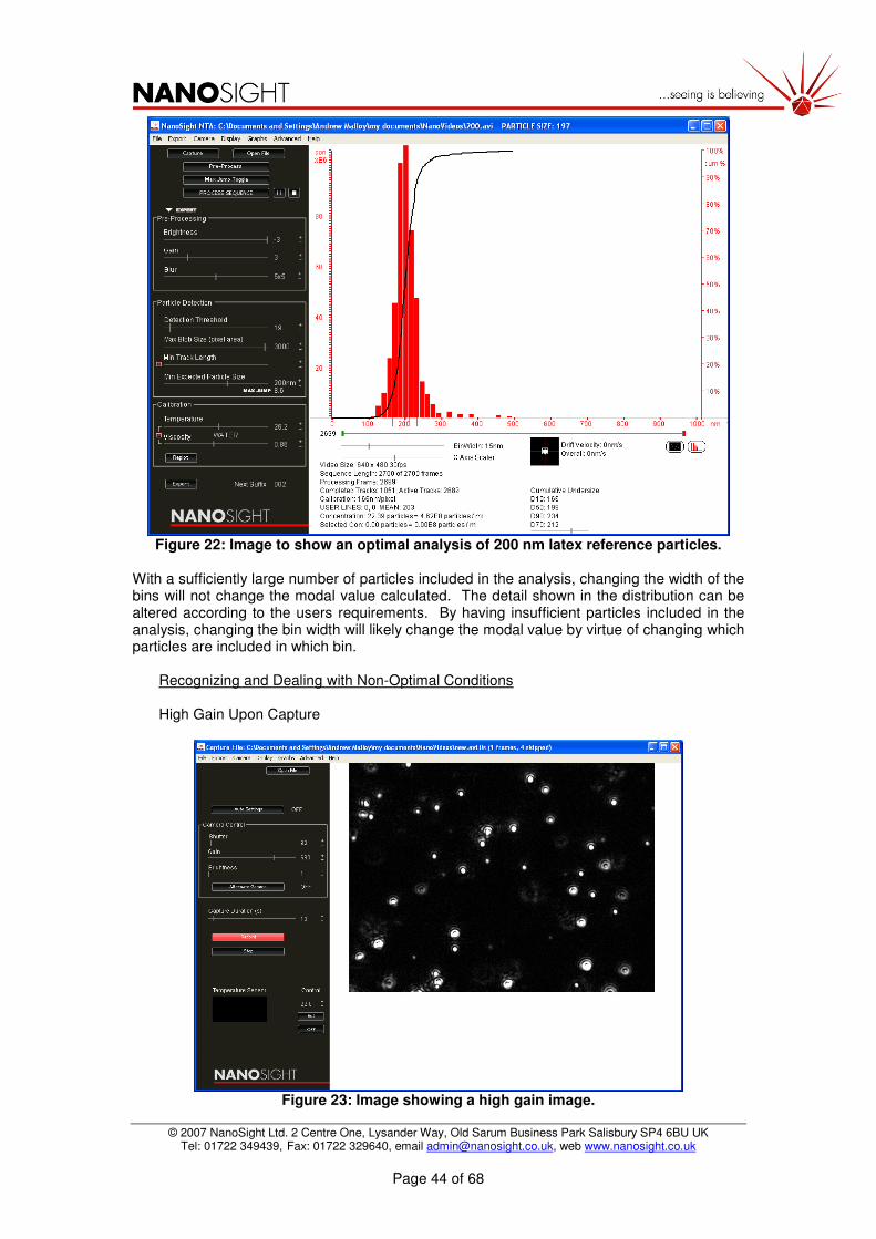
© 2007 NanoSight Ltd. 2 Centre One, Lysander Way, Old Sarum Business Park Salisbury SP4 6BU UK Tel: 01722 349439, Fax: 01722 329640, email [email protected], web www.nanosight.co.uk
Page 44 of 68
Figure 22: Image to show an optimal analysis of 200 nm latex reference particles.
With a sufficiently large number of particles included in the analysis, changing the width of the bins will not change the modal value calculated. The detail shown in the distribution can be altered according to the users requirements. By having insufficient particles included in the analysis, changing the bin width will likely change the modal value by virtue of changing which particles are included in which bin.
Recognizing and Dealing with Non-Optimal Conditions
High Gain Upon Capture
Figure 23: Image showing a high gain image.

© 2007 NanoSight Ltd. 2 Centre One, Lysander Way, Old Sarum Business Park Salisbury SP4 6BU UK Tel: 01722 349439, Fax: 01722 329640, email [email protected], web www.nanosight.co.uk
Page 45 of 68
As can be seen from fig 20. a high gain image can suffer from a large amount of background noise and the diffraction patterns can clearly be seen around a number of particles. Although the original image is noisy, the software filters in the analysis phase can be used to deal with the image.
Figure 24: Image showing the software filters necessary to deal with a high gain image.
High Shutter Upon Capture
Figure 22: Image showing high shutter image of 200 nm latex reference spheres.
Brightness: -70. The brightness can be used to counteract the high gain used to capture the image. Gain: 1. As the image was captured at a high gain no further gain is required in processing. Blur 7x7 Used to blur rings as a result of increased gain at capture. Blob size is set high to include larger footprint particles resulting from high gain

© 2007 NanoSight Ltd. 2 Centre One, Lysander Way, Old Sarum Business Park Salisbury SP4 6BU UK Tel: 01722 349439, Fax: 01722 329640, email [email protected], web www.nanosight.co.uk
Page 46 of 68
As can be seen from Fig 22, an image captured from a high shutter image produces a blurry image. As is explained in Step 1, long shutter times can result in problems with particle centering due to blurred particles. Although a high gain image vs a high shutter image do not look dissimilar, high shutter images will result in accuracies in particle sizing whereas the high gain images will not. In practice the user should not select shutter values in excess of 1000.
Figure 23: Particle distribution produced by a high shutter capture.
As can be seen from Fig.23 the modal value calculated by the analysis is too high due to the excessive shutter used to capture the image. As a general rule, the shutter should be kept to the minimum value to allow visualisation of the particles but minimising particle blurring.
Incorrect Sample Concentrations
Figure 24: (a) Too high concentration of particles (b) Too low concentration of particles. As can be seen from Fig.24, the system has certain requirements regarding sample concentration. Ideally the sample should contain between 10
6 and 10
8 particles per ml
dependant upon the size of the particles. Fig.24(a) represents an over concentrated image and represents a sample concentration of around 10
10 particles per ml. Such images
(a) (b)

© 2007 NanoSight Ltd. 2 Centre One, Lysander Way, Old Sarum Business Park Salisbury SP4 6BU UK Tel: 01722 349439, Fax: 01722 329640, email [email protected], web www.nanosight.co.uk
Page 47 of 68
represent a problem in that the rate at which the particles cross over is unacceptable, hence there is a possibility that the software will erroneously join tracks from adjacent particles. Fig.25(a) shows the resulting distribution from an over concentrated sample. As can be seen the modal value produced is slightly lower than should be expected – due to the increased cross over rate of the particles. Fig.24(b) shows a sample with too few particles are represents a sample concentration in the order of 10
6 particles per ml. Fig.25(b) shows the resulting analysis from such a sample. As
can be seen, insufficient particles were analysed to produce a stable distribution of particle sizes. If possible, such a sample should be increased in concentration or the analysis run for an extended period of time in order to increase the data set.
Figure 25: Particle size distribution of 200 nm Latex spheres (a) too concentrated sample (b) too dilute sample.
100 nm Reference Latex Spheres
Figure 26: Ideal image of 100 nm Latex Reference Particles.
(b) (a)

© 2007 NanoSight Ltd. 2 Centre One, Lysander Way, Old Sarum Business Park Salisbury SP4 6BU UK Tel: 01722 349439, Fax: 01722 329640, email [email protected], web www.nanosight.co.uk
Page 48 of 68
Figure 27: Ideal setting used to analyse 100 nm latex reference spheres.
The software filters should be altered in the order in which they are listed going down the screen. The brightness should be reduced to a point so as any background noise is removed from the image. Following this, the gain should be used to increase the brightness of the very dimmest particles. Next the blur should be applied in order that the false centres which are located around the brightest particles are removed. At the start of the analysis the detection threshold should be increased to maximum to remove all centres from the particles. This allows the user to better determine the effect of the software filters as they are changed without interference form the red centres. Having varied the brightness, gain and blur, the detection threshold can be reduced down to a level where the dimmest particles are included in the analysis and not the background noise. The max blob size should then be increased to a level so that all of the largest particles are included in the analysis. If the auto-capture settings have been used then the automatic processing settings can also be employed to produce an ideal distribution for mono-dispersed 100nm particles.
Brightness: -13. The brightness can be used to counteract the gain used brighten image. Gain: 3. Used to increase difference between dim particle and noise Blur 3x3. Few rings therefore little blur needed Min Particle Size – Set to 100nm with corresponding Max jump of 12.1

© 2007 NanoSight Ltd. 2 Centre One, Lysander Way, Old Sarum Business Park Salisbury SP4 6BU UK Tel: 01722 349439, Fax: 01722 329640, email [email protected], web www.nanosight.co.uk
Page 49 of 68
Figure 28: Particle size distribution produced from ideal image of 100 nm reference
spheres.
Effect of Time of Capture on 100 nm Particles
Figure 29: Images to show how length of capture influences the calculated size for 100
nm latex spheres. As can be seen from Fig.29, the length of capture can influence the particle size distribution should not enough particles be analysed. As can be seen the difference between the 60
60 Seconds
10 Seconds
30 Seconds
5 Seconds
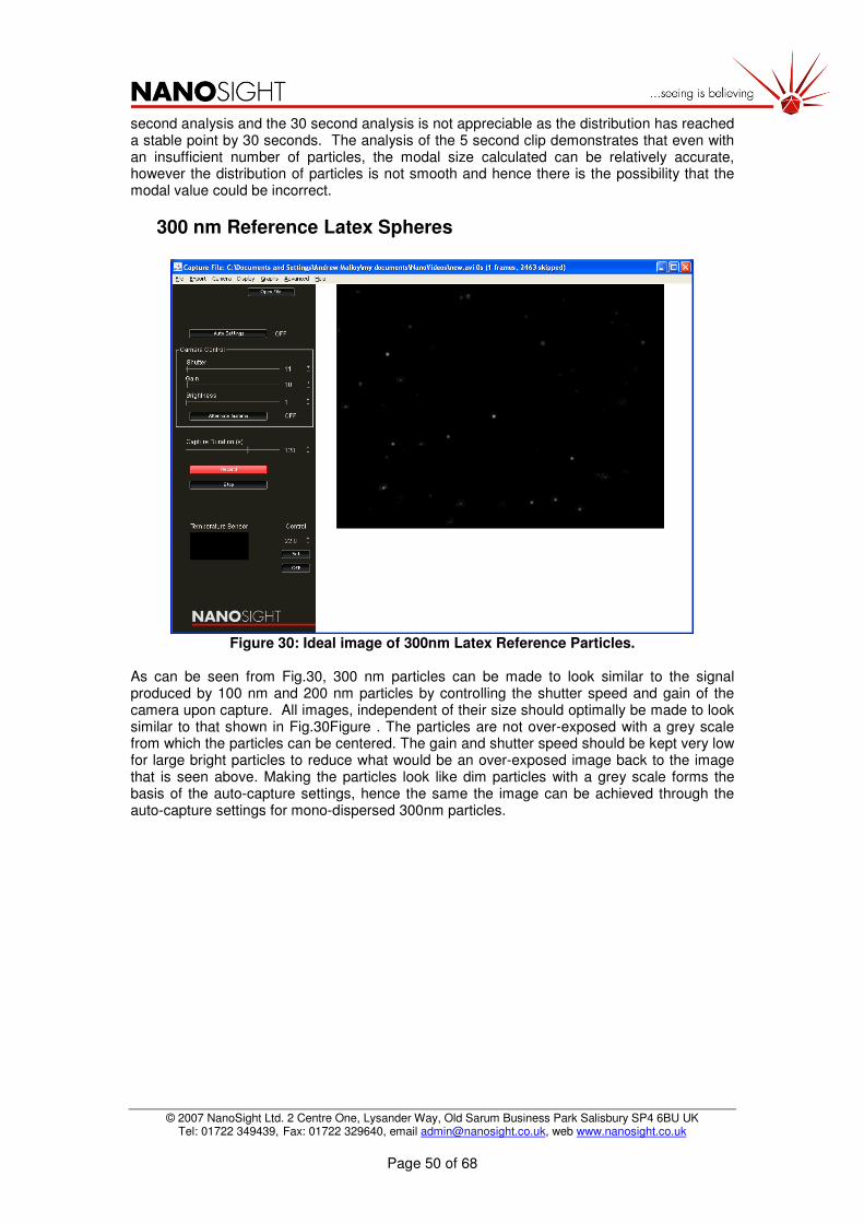
© 2007 NanoSight Ltd. 2 Centre One, Lysander Way, Old Sarum Business Park Salisbury SP4 6BU UK Tel: 01722 349439, Fax: 01722 329640, email [email protected], web www.nanosight.co.uk
Page 50 of 68
second analysis and the 30 second analysis is not appreciable as the distribution has reached a stable point by 30 seconds. The analysis of the 5 second clip demonstrates that even with an insufficient number of particles, the modal size calculated can be relatively accurate, however the distribution of particles is not smooth and hence there is the possibility that the modal value could be incorrect.
300 nm Reference Latex Spheres
Figure 30: Ideal image of 300nm Latex Reference Particles.
As can be seen from Fig.30, 300 nm particles can be made to look similar to the signal produced by 100 nm and 200 nm particles by controlling the shutter speed and gain of the camera upon capture. All images, independent of their size should optimally be made to look similar to that shown in Fig.30Figure . The particles are not over-exposed with a grey scale from which the particles can be centered. The gain and shutter speed should be kept very low for large bright particles to reduce what would be an over-exposed image back to the image that is seen above. Making the particles look like dim particles with a grey scale forms the basis of the auto-capture settings, hence the same the image can be achieved through the auto-capture settings for mono-dispersed 300nm particles.

© 2007 NanoSight Ltd. 2 Centre One, Lysander Way, Old Sarum Business Park Salisbury SP4 6BU UK Tel: 01722 349439, Fax: 01722 329640, email [email protected], web www.nanosight.co.uk
Page 51 of 68
Figure 31: Image showing the ideal software setting used to analyse 300 nm particles. As can be seen from Fig.31 the settings used to analyse the image produced by the 300 nm particles are largely similar to those used to analyse the 200 nm particles. This is largely due to the fact that the camera controls are used to produce, similar, optimal images across the range of particle sizes.
Figure 32: Particle size distribution produced from ideal image of 300 nm reference
spheres.
Min Track length – Auto setting (red box clicked) Min Particle Size Expected – 300 with corresponding Max Jump of 6.5 pixels. Max Blob Size 3000 – to include larger footprint particles. Blur 5x5 to blur any rings around brighter particles.
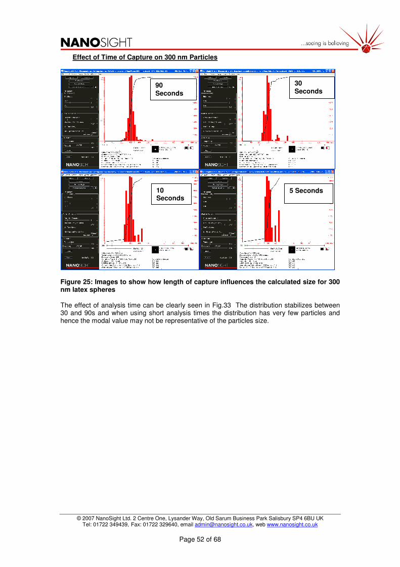
© 2007 NanoSight Ltd. 2 Centre One, Lysander Way, Old Sarum Business Park Salisbury SP4 6BU UK Tel: 01722 349439, Fax: 01722 329640, email [email protected], web www.nanosight.co.uk
Page 52 of 68
Effect of Time of Capture on 300 nm Particles
Figure 25: Images to show how length of capture influences the calculated size for 300 nm latex spheres The effect of analysis time can be clearly seen in Fig.33 The distribution stabilizes between 30 and 90s and when using short analysis times the distribution has very few particles and hence the modal value may not be representative of the particles size.
90
Seconds
10 Seconds
5 Seconds
30 Seconds

© 2007 NanoSight Ltd. 2 Centre One, Lysander Way, Old Sarum Business Park Salisbury SP4 6BU UK Tel: 01722 349439, Fax: 01722 329640, email [email protected], web www.nanosight.co.uk
Page 53 of 68
400 nm Reference Latex Spheres
Figure 34: Ideal image of 400 nm Latex Reference Particles.
By using the camera settings the particles can be reduced to small points of light which can be centered very easily. The shutter speed and gain is set extremely low and a long analysis time is used. By using a long analysis time we are ensuring that the distribution produced is stable and accurate for slow moving 400 nm particles.
Figure 35: Image showing the ideal software setting used to analyse 400 nm particles.
Min Particle Size – 400nm and corresponding Max Jump of 5.7 pixels.
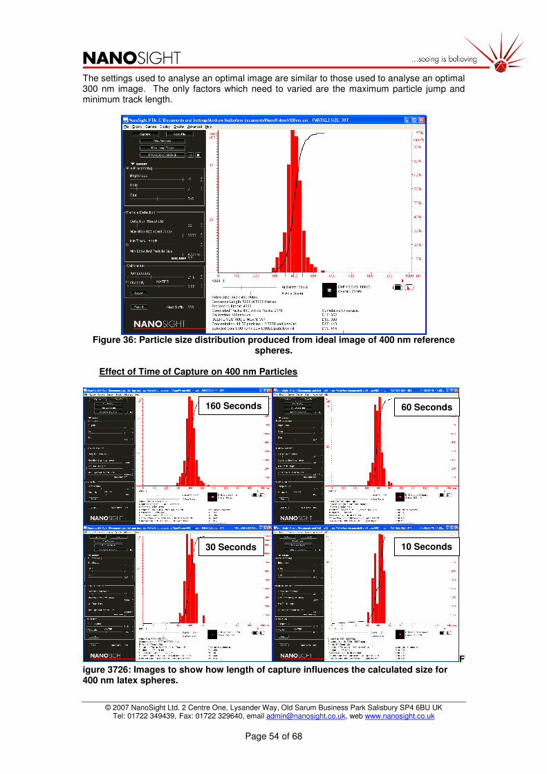
© 2007 NanoSight Ltd. 2 Centre One, Lysander Way, Old Sarum Business Park Salisbury SP4 6BU UK Tel: 01722 349439, Fax: 01722 329640, email [email protected], web www.nanosight.co.uk
Page 54 of 68
The settings used to analyse an optimal image are similar to those used to analyse an optimal 300 nm image. The only factors which need to varied are the maximum particle jump and minimum track length.
Figure 36: Particle size distribution produced from ideal image of 400 nm reference
spheres.
Effect of Time of Capture on 400 nm Particles
Figure 3726: Images to show how length of capture influences the calculated size for 400 nm latex spheres.
160 Seconds 60 Seconds
30 Seconds 10 Seconds

© 2007 NanoSight Ltd. 2 Centre One, Lysander Way, Old Sarum Business Park Salisbury SP4 6BU UK Tel: 01722 349439, Fax: 01722 329640, email [email protected], web www.nanosight.co.uk
Page 55 of 68
30 nm Gold Colloid
Figure38: Typical image that would be seen when analysing 30 nm gold colloid.
As can be seen from the above image particles in the order of 30nm scatter light very poorly and as a result the image produced is very dim. Gold is an effective scatter of light and hence gold particles will appear brighter than a similarly sized particle of a low refractive index. Using the camera controls the particles can be made to appear brighter than in the image above, however the accuracy of the results may suffer. The above image has been captured at maximum Gain (680) and a moderate Shutter speed (480). By increasing the shutter to maximum the particles could be made to appear brighter however particle blurring would occur and the result would suffer. The image should therefore be captured such that the particles appear fairly dim, as above, and then the image can be gained in the image processing part of the analysis.

© 2007 NanoSight Ltd. 2 Centre One, Lysander Way, Old Sarum Business Park Salisbury SP4 6BU UK Tel: 01722 349439, Fax: 01722 329640, email [email protected], web www.nanosight.co.uk
Page 56 of 68
Figure39: Optimum settings to analyse 30 nm gold colloids.
A Gain of 6 has been used to allow better visualisation of the dimmest particles. As a result of gaining the image, the background noise will also be gained. Reducing the Brightness to -13 will remove the background noise form the analysis. The Detection Threshold should be reduced (26) to include the dimmest particles in the analysis and the Maximum Blob Size increased (3000) to include the largest particles in the analysis.

© 2007 NanoSight Ltd. 2 Centre One, Lysander Way, Old Sarum Business Park Salisbury SP4 6BU UK Tel: 01722 349439, Fax: 01722 329640, email [email protected], web www.nanosight.co.uk
Page 57 of 68
As the particles have very rapid movement under Brownian motion they will not exist in the field of view for extended periods of time. As a result if a long Minimum Track Length is set, no particles will be included in the analysis. By using the auto setting for Minimum track length the software will automatically set a short tracking duration for these fast moving 30nm particles. Again the software should be told that the sample contains 30nm particles by selecting this value in the Min Expected Particle Size.
Figure 40: Particle size distribution for 30 nm Gold Colloid

© 2007 NanoSight Ltd. 2 Centre One, Lysander Way, Old Sarum Business Park Salisbury SP4 6BU UK Tel: 01722 349439, Fax: 01722 329640, email [email protected], web www.nanosight.co.uk
Page 58 of 68
Poly-Dispersed Sample of 100 nm and 200 nm Polystyrene Reference Spheres
Figure 41: Ideal image of 100 nm and 200 nm poly-dispersed sample.
As can be seen from Fig. 41, the sample has been treated as if it where a 100 nm sample. The camera controls have been used to reduce the 100 nm particles to dim discs as in Worked Example 2. As a result the 200 nm particles appear much brighter in the image and hence have been captured in non-optimal conditions. The limitations of the technique (when analysing poly-dispersed samples) depends largely upon the scattering efficiencies of the two particle populations. If the two populations of particles have vastly different scattering characteristics, i.e. 100 nm and 600 nm, then the user will not be able to capture both particle populations at optimal settings. If the camera settings are used to optimally capture the 600 nm particles then the 100 nm particles will not be visible, conversely, if the camera controls are used to optimally capture the 100 nm particles then the image produced by the 600 nm particles will be oversaturated and difficult to centre. In situations such as these, two-step analyses will produce the most accurate results. The system should be used to optimally capture an image from the 600 nm particles and an analysis performed. The sample should then be physically filtered to remove the large particles and a second analysis performed on the small particle population. Poly-dispersed systems which have particle populations that are closely matched in size present a different problem. Now the broadness of the distribution is the limiting factor when trying to resolve particle peaks. The distribution produced by this technique is slightly broader than a distribution produced by techniques such as PCS. Since Brownian motion is a random process, the software tracks the particles over a number of frames and calculates the average distance it has moved over that time period. If the particles were tracked to infinity, the average distance moved by a particle would be accurately related to its size. The particles tracked in this technique however are tracked for a finite time and hence there is the possibility that the particle size produced for a single particle may be slightly larger or smaller than its actual size had it been tracked to infinity, and hence the distribution produced is broadened. As a ‘rule of thumb’, particles which are no larger than 4 times the size of another population of particles can be resolved (limited by the quality of the image produced) and particles no smaller than 1.5 times the size of another population of particle can be resolved (limited by the broadness of the distribution).

© 2007 NanoSight Ltd. 2 Centre One, Lysander Way, Old Sarum Business Park Salisbury SP4 6BU UK Tel: 01722 349439, Fax: 01722 329640, email [email protected], web www.nanosight.co.uk
Page 59 of 68
Figure 42: Ideal settings used to analyse 100 nm + 200 nm mixed sample.
• Gain 2: Makes the dimmest 100nm particles more visible – depending upon the image this may not be necessary as it also gains the larger particles.
• Brightness: -9 – Removes any background noise and flare around the particles.
• Blur: 5x5 Allows the centres of the largest particles to be accurately found.
• Detection Threshold: 28 – To pick up the dimmest particles.
• Max Blob Size: 3000 Increased to include the largest particles in the analysis
• Min Track Length: Auto-settings.
• Min Expected Size - 100nm.

© 2007 NanoSight Ltd. 2 Centre One, Lysander Way, Old Sarum Business Park Salisbury SP4 6BU UK Tel: 01722 349439, Fax: 01722 329640, email [email protected], web www.nanosight.co.uk
Page 60 of 68
Figure 43: Particle size distribution produced for sample of 100 nm and 200 nm
particles.

© 2007 NanoSight Ltd. 2 Centre One, Lysander Way, Old Sarum Business Park Salisbury SP4 6BU UK Tel: 01722 349439, Fax: 01722 329640, email [email protected], web www.nanosight.co.uk
Page 61 of 68
h. Recommended capture and analysis settings Ideal camera settings for optimal image acquisition*:
Particle Size Shutter Gain Brightness Alternate Gamma
Capture Duration
30nm 500 680 1 Possibly 20-30s
100nm 300 580 1 No 30-40s
200nm 110 0 1 No 60-90s
300nm 10 0 1 No 90-120s
400nm 10 0 1 No 120-150s
100+200nm 300 50 1 Possibly 90s
*Note that the values (especially for shutter and gain) indicated below are very approximate and should be analysed on a case-by-case basis. Once an optimal image has been acquired using the above settings (or similar to) the following settings can be used to produce an optimal analyses*.
Particle Size
Brightness Gain Blur Detection Threshold
Max Blob Size
Min Track
Length
Min Size Expected
30nm Gold -13 6 3x3 25 3000 Auto 30
100nm -10 3 3x3 20 3000 Auto 100
200nm -13 3 5x5 20 3000 Auto 200
300nm -7 3 5x5 30 3000 Auto 300
400nm -7 2 5x5 30 3000 Auto 400
100+200nm -9 2 5x5 25 3000 Auto 100
*Note that the values (especially for brightness and detection threshold) indicated below are very approximate and should be analysed on a case-by-case basis.

© 2007 NanoSight Ltd. 2 Centre One, Lysander Way, Old Sarum Business Park Salisbury SP4 6BU UK Tel: 01722 349439, Fax: 01722 329640, email [email protected], web www.nanosight.co.uk
Page 62 of 68
8. Frequently Asked Questions a. Fundamental questions
How much light is scattered by a particle? The particles that we size are generally in the Rayleigh or Rayleigh-Debye-Gans scattering regime. As an approximation, the Rayleigh regime will be briefly discussed. In this case the efficiency of light scattering is given by:
Therefore the factors affecting the amount of light scattered are:
• d is the particle diameter. If you double the particle size you increase the power of light scattered by a factor of 64.
• λ is the wavelength of light. If you half the wavelength of light you increase the scattering by a factor of 16.
• n is the ratio of the particle refractive index to the solvent refractive index. For
example for latex particles (ref. ind. 1.59) in water (ref. ind. 1.33), n is 1.195 and the factor is 0.0157.
However for the case of gold (ref. ind. 0.14-3.7i) in water n is 0.1053 + 2.7820i and
is 2.3, a factor of 147 greater than for the latex particles. The amount of light scattered is also directly proportional to the intensity of incident illumination.
How long is a sample stable for? Will the nanoparticles aggregate? The science behind dispersion chemistry is not simple and we do not claim that we can stop your particles aggregating. We often use a little ultrasound but usually look to the customer to provide a protocol to disperse and stabilize the system. We also refer to ISO 14887 Sample Preparation – Dispersing procedures for powders and liquids. However if the sample is at suitable viewing concentration then the injection and time to the start of the measurement can be less than 30 seconds and a measurement can take as little as 10 seconds. Therefore our system can be used to monitor aggregation if the process is sufficiently slow (e.g. takes longer than 5 minutes). Note also that if a sample settles to a significant degree over an hour or two, this strongly
indicates that it containes particles in the µm range and which are therefore not true colloidal nanoparticles and therefore may be at the extreme of our analytical capability.

© 2007 NanoSight Ltd. 2 Centre One, Lysander Way, Old Sarum Business Park Salisbury SP4 6BU UK Tel: 01722 349439, Fax: 01722 329640, email [email protected], web www.nanosight.co.uk
Page 63 of 68
The particles are only being imaged in two dimensions, but they must be moving in three dimensions. Is this a problem? No. The Stokes-Einstein theory that is used to calculate the particles size from the particle motion can take into account whether two or three dimensions are tracked (see equations below).
How does a larger particle (such as an advanced agglomerate or contaminant) affect the measurement? Unlike other light scattering techniques we are not strongly affected by large contaminants. This is because we visualise individual particles. Whilst an unusually large particle will scatter far more than the primary particles, its scattered light will be confined to and tracked only in a discrete region of the image.
Can I use different solvents in your device? Yes. Whilst the system is typically optimised for water as the solvent we have got good results from other solvents. As an indication solvents with a refractive index up to a value of approximately 1.45 can be analysed. For solvents with a higher refractive index please consult NanoSight. Water is 1.33 and a water-optimised LM unit will work up to about Rf of 1.4. Above this, a unit optimised from 1.40 should work up to 1.52, but best way is to try this.
What is the upper size limit of particles that can be sized by your system? The upper size limit of 500nm that we suggest is an approximation and dependent on particle type. The NanoSight NTA technique analyses the movement of a particle undergoing Brownian motion by tracking in time the spot of light it scatters. For large particles:
1. The diffusion of the particle becomes increasing limited making the accurate determination of its mean displacement progressively less accurate.
2. For dense (metal or metal oxide) particles, sedimentation rates begin to exceed the limited Brownian motion.
3. The spot of light becomes so large and its edges so variable between frames, that identifying its centre becomes increasingly difficult leading to centring errors which are as large as the particle’s movement.
4. the numbers of particles that can be viewed at any one time decreases (because of the amount of light they scatter
These effects get progressively larger as particle size increases so there is no specific limit to our upper size range. This upper limit will depend on the nature of the system. In practice, for low density and low Ri particles such as polystyrene microspheres their buoyancy and weaker scattering allow them to remain Brownian movers with easily identifiable centres and the upper size limit is 600-800nm or above. For dense, high Ri particles such as gold, their rapid sedimentation rate and excessive scattering restricts the upper size at which they can be analysed to approx <200nm.
What is the smallest particle that can be analysed? The minimum size of particle that is detectable depends on the scattering being sufficiently strong. To understand this question better see ‘How much light does a particle scatter?’. As a general guide:
• Low Ri (e.g. biological/polymer) will be detectable down to approximately 30-40nm.
• Higher refractive particles (e.g. ceramics, metal oxides) will be detectable down to approximately 15-25nm.
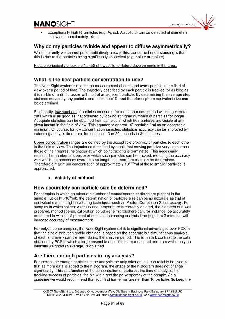
© 2007 NanoSight Ltd. 2 Centre One, Lysander Way, Old Sarum Business Park Salisbury SP4 6BU UK Tel: 01722 349439, Fax: 01722 329640, email [email protected], web www.nanosight.co.uk
Page 64 of 68
• Exceptionally high Ri particles (e.g. Ag sol, Au colloid) can be detected at diameters as low as approximately 10nm.
Why do my particles twinkle and appear to diffuse asymmetrically? Whilst currently we can not put quantitatively answer this, our current understanding is that this is due to the particles being significantly aspherical (e.g. oblate or prolate) Please periodically check the NanoSight website for future developments in the area..
What is the best particle concentration to use? The NanoSight system relies on the measurement of each and every particle in the field of view over a period of time. The trajectory described by each particle is tracked for as long as it is visible or until it crosses with that of an adjacent particle. By determining the average step distance moved by any particle, and estimate of Dt and therefore sphere equivalent size can be determined. Statistically, low numbers of particles measured for too short a time period will not generate data which is as good as that obtained by looking at higher numbers of particles for longer. Adequate statistics can be obtained from samples in which 50+ particles are visible at any given instant in the field of view. This equates to approx 10
6 particles / ml as an acceptable
minimum. Of course, for low concentration samples, statistical accuracy can be improved by extending analysis time from, for instance, 10 or 20 seconds to 3-4 minutes. Upper concentration ranges are defined by the acceptable proximity of particles to each other in the field of view. The trajectories described by small, fast moving particles very soon cross those of their nearest neighbour at which point tracking is terminated. This necessarily restricts the number of steps over which such particles can be tracked, reducing the accuracy with which the necessary average step length and therefore size can be determined. Therefore a maximum concentration of approximately 10
9-10/ml of these smaller particles is
approached.
b. Validity of method
How accurately can particle size be determined? For samples in which an adequate number of monodisperse particles are present in the sample (typically >10
9/ml), the determination of particles size can be as accurate as that of
equivalent dynamic light scattering techniques such as Photon Correlation Spectroscopy. For samples in which solvent viscosity and temperature is correctly entered, the diameter of a well prepared, monodisperse, calibration polystyrene microsphere can, for instance, be accurately measured to within 1-2 percent of nominal. Increasing analysis time (e.g. 1 to 2 minutes) will increase accuracy of measurement. For polydisperse samples, the NanoSight system exhibits significant advantages over PCS in that the size distribution profile obtained is based on the separate but simultaneous analysis of each and every particle seen during the analysis period. This is in stark contrast to the data obtained by PCS in which a large ensemble of particles are measured and from which only an intensity weighted (z-average) is obtained.
Are there enough particles in my analysis? For there to be enough particles in the analysis the only criterion that can reliably be used is that as more data is added to the histogram, the shape of the histogram does not change significantly. This is a function of the concentration of particles, the time of analysis, the tracking success of particles, the bin width and the polydispersity of the sample. As a guideline we would recommend that your first frame has greater than 10 particles (to keep the

© 2007 NanoSight Ltd. 2 Centre One, Lysander Way, Old Sarum Business Park Salisbury SP4 6BU UK Tel: 01722 349439, Fax: 01722 329640, email [email protected], web www.nanosight.co.uk
Page 65 of 68
experimental time required to a reasonable length) and less than 100 (otherwise there is a significant risk of particle tracks being discarded due to ambiguity about their origin). As a rough guideline a 30s movie clip of monodisperse 100nm particles will have sufficient number of tracks with a bin width of 20nm. Another guideline value to use is that the peak bin should have a frequency greater than 50.
Why do you not use an increased frame rate to obtain more data? Whilst an increased frame rate (for example 60fps) would give more data, it also means that the exposure time for the camera is necessarily shorter which means weaker scattering particles may not be observed. Similarly, shorter sampling rates results in shorter distances being measured with a resulting loss in accuracy of estimation of motion. We have found that our current 30fps system is adequate for all particles visible in our system.
How well can different sizes be resolved from each other in a mixture? Under ideal conditions (two very monodisperse populations of similar type and of similar number density, we have achieved resolutions of less than a factor of 1.25. Should either of these populations exhibit any significant breadth of distribution, their diffusion coefficients become too similar to differentiate easily and the size ratios at which they can be resolved will also increase accordingly. In practice, for all but the most well prepared of calibration particles, resolution of mixtures of particles within a 1.5 diameter ratio can rarely be achieved with a high degree of confidence. This, however, represents a significant improvement on the resolutions routinely achievable with PCS which, in practice cannot resolve systems by greater than a factor of 2.
How reproducible is the result? Given the statistical nature of analysis of a population of particles, reproducibility is a function of the numbers of particles measured over a given period of analysis. For optimum concentrations of monodisperse samples containing no contaminating aggregates, results reproducible to within approx 2-3% can be achieved in a comparatively short time (e.g. 10-20seconds). Clearly, for low concentrations of particles exhibiting a range of particle sizes, extended analysis periods will be required to obtain reproducibility of results. Note that analysis times need to be increased for larger particle diameters to achieve similar reproducibilities.
Can you use NanoSight system to obtain concentration measurement? Whilst the NTA software suite does produce a number distribution, this is not an absolute function of the sample concentration. There are a number of reasons for this which are addressed in a number of the following questions.
Small particles are not tracked as long as large particles. Is this a problem? The LM10/LM20 systems will size the particles that can be centred for a sufficient number of consecutive frames (min track length). Therefore if the particles are tracked for fewer frames than this they will not be counted. The minimum track length should be set sufficiently low to track the smallest particles. The minimum track length is therefore set by the smallest particles in the sample. We suggest the following rough guidelines be followed; however this setting is also dependent on the particle type, concentration and analysis time being sufficient to obtain reasonable numbers.
Minimum particle size in sample (nm)
Minimum track length setting
<50 5
100 10

© 2007 NanoSight Ltd. 2 Centre One, Lysander Way, Old Sarum Business Park Salisbury SP4 6BU UK Tel: 01722 349439, Fax: 01722 329640, email [email protected], web www.nanosight.co.uk
Page 66 of 68
200 15
300 20
400+ 25
c. User questions
How wide a range of particle sizes can be analysed at the same time? When the range of particle sizes (and/or refractive indices or indeed relative number concentration) becomes too wide, no single choice of camera and software settings (gain, shutter speed, threshold, etc.) will allow all particles present to be analysed with equal accuracy. While a high number of small particles may be measured even when a certain number of larger particles (aggregates or contaminants) are present, when the number of such large particles becomes excessive, their high population and large light scattering footprints can begin to obscure the presence of the smaller population. Of course, the point at which the results become non-representative depends strongly on the relative numbers of each population and the size differential between them. For instance, in selecting a low camera gain setting which is optimal for the larger sized fraction, such settings may be inappropriate for the smaller size which accordingly, will be missed in the analysis. Similarly, a setting at which small particles can be visualised may well result in excessive signal from the larger population. In practice, for polystyrene microspheres, a mixture of 100nm and 400nm particles can be analysed if the numbers of each size are approximately 2:1. Conversely, 100nm particles will be increasingly difficult to analyse if 400nm particles are present at number ratios in excess of 1:2. Visual inspection of the sample by the microscope can often allow the user to see the presence of lower numbers of smaller particles in a sample but at which exist at concentrations which become too low for the analytical programme to measure them accurately. This ability is, however, a significant advantage over other particle sizing techniques (such as photon correlation spectroscopy) in which the user is effectively working blind and frequently may be unaware of the presence of smaller particles. At this stage, physical removal of the larger sized fraction by either filtration or centrifugation is appropriate and will allow the smaller population to be reanalysed with far higher accuracy.
How do I calibrate my system? Our method of particle tracking is absolute as it is based on dynamic measurements in the time domain. The only paramters that need to be known are the solvent temperature and the viscosity of the solvent at that temperature. Therefore there is no calibration required other than ensuring the field of view of the camera is correct. In all systems we supply this is factory set and not user adjustable. For estimation of paricle number concentration, however, it is advisable that the user use another technique to determine the number concentration of a sample, using this value to calibrate the NanoSight system for counting purposes only
How long does the sample temperature take to equilibrate? The sample volume, at approx 500 ul, is smaller than is typically used in other light scattering measurements. Therefore the time taken for the liquid temperature to equalise with that of the metal housing is relatively small. 30s should be adequate time for temperature equilibration.
I am still seeing a significant flow of particles, but have waited longer than 30s. Why is this? There are three possibilities why this may be so and these are listed below in increasing likelihood:
1) Sample leakage. When setting up, it is imperative that the optical flat surface is correctly seated in the viewing unit, the sealing ‘O’ ring is correctly seated in the top plate and that the top plate has been brought into contact with the optical flat surface horizontally. Refer to the manual for a description of these processes.

© 2007 NanoSight Ltd. 2 Centre One, Lysander Way, Old Sarum Business Park Salisbury SP4 6BU UK Tel: 01722 349439, Fax: 01722 329640, email [email protected], web www.nanosight.co.uk
Page 67 of 68
2) The beam has become incorrectly aligned and light is being absorbed by the optical flat surface. If this is the case check that the flat was seated correctly in the
3) The particles are very large and very absorbing causing heating in the cell 4) The solvent you are using is very absorbing, which is causing convective currents.
Small particles are not as bright as large particles and I find it hard to track both at the same time, what should I do? If after using the optimum capture settings, the processing settings can either not be adjusted such that the smallest particles can be seen or they can be seen but can not be successfully centred on, it may be necessary to carry out a two-pass experiment. This would involve first sizing the large particles then subsequently filtering the sample and recording a movie of the smaller particles. As a guideline, if the smallest particles are a factor of three smaller (in terms of diameter) than the largest particles these may be difficult to analyse if present in equal numbers.
I want to put my movies in a presentation but they are very large. Can I compress these? Yes, the easiest way we have found to do this is using the Windows Movie Maker software that comes with, for example, Windows XP. The settings we use are all the default ones and this we find perfectly sufficient. Note, you will not be able to re-analyse video clips following compression
Is it possible I could have blocked the inlet outlet ports with particles? Particles over 100 microns may block the inlet ports.
d. Specification questions
What are the space requirements of the system? The system requires room for a desktop PC and (in addition) approximately 0.4 x 0.4m of bench space
What are the dimensions of the sample chamber? Cell volume: Approximately 0.25 ml. Cell depth: 0.9mm
How long is the lifetime of laser source in LM10 unit? 10,000 hours specified by manufacturer
How long can I leave a sample in the cell? Providing that the system that you are looking at is suitably stable, the water will not evaporate over a period of many days. Note however, that some particle types will ‘plate out’ on the internal surfaces of the sample chamber (through, for instance, electrostatic interactions) and may increasingly contribute to noise within the system. Also, on re-analysis, there may be a significant reduction in particle number.
Is the system safe? Yes. The system is a Class I Laser product if used correctly according to the manufacturer’s instructions as it has a fail-safe mechanism.

© 2007 NanoSight Ltd. 2 Centre One, Lysander Way, Old Sarum Business Park Salisbury SP4 6BU UK Tel: 01722 349439, Fax: 01722 329640, email [email protected], web www.nanosight.co.uk
Page 68 of 68
What is the unit made of? The parts of the LM10 unit in contact with the sample are made of glass, stainless steel and the plastic of the inlet/outlet ports. The seal is Viton.
Do I need an anti-vibration table for the system? No. Any solid and heavy surface that is suitable for conventional microscopy will suffice though extended analyses will be affected by significant and continuous vibration.
9. Troubleshooting and Fault finding
Symptom Cause Remedial Action
No Optical beam visible
Power not connected No sample in cell Sample too dilute Laser beam misaligned Laser not working
Check and Connect Switch on. Fill cell Increase sample concentration Re-alignment required. Refer to manufacturer Replacement laser required. Refer to Manufacturer
Presence or formation of air/gas bubbles
Incorrect sample introduction Dissolved gas in (cold) sample Dirty window or optical element
Introduce sample slowly while tilting device De-gas sample before analysis Clean as instructed above
Scratched metal surface on optical flat
Incorrect cleaning Inspect and Replace
Unable to detect or resolve particles
Sample too concentrated Sample too dilute Focus incorrect Mis-aligned microscope Particles too small
Dilute and re-analyse Use higher concentration sample Adjust accordingly Ensure beam is central to microscope field of view Discuss with NanoSight
Large light scattering centres present
Bubble formation Contaminant particles in sample
De-gas sample Filter or Centrifuge sample
High background
Optical surfaces contaminated Dissemble and clean as instructed