Auctions with Bid Credits and Resale∗

Simon Loertscher† Leslie M. Marx‡

June 2, 2016

Abstract

Bid credits favoring subsets of bidders are routinely imposed on auctions and procurement

auctions. These bid credits result in inefficient auction outcomes, which create pressure for

post-auction resale or, in a procurement context, for subcontracting. We show that the

presence of resale, in turn, affects bidding strategies in such a way that auction outcomes

are more likely to be inefficient and less informative, making it harder for resale to correct

inefficiencies. The negative effects of bid credits and resale can be mitigated through direct

restrictions on resale, tight caps on credits, reserve prices, anonymous bidding, and enhanced

competition.

Keywords: designated entities, spectrum license auctions

JEL Classification: C72, D44, L13

∗We thank Jonathan Levy, Eliot Maenner, Ilya Segal, Martha Stancill and and seminar participants at DukeUniversity, the Econometric Society Australasian Meeting 2014 in Hobart, and the ESEI/UTS Conference inHonor of John Ledyard for valuable comments and suggestions. We thank Federico Mini and Hoel Wiesner forvaluable research assistance.

†Department of Economics, Level 4, FBE Building, 111 Barry Street, University of Melbourne, Victoria 3010,Australia. Email: simonl@unimelb.edu.au.

‡The Fuqua School of Business, Duke University, 100 Fuqua Drive, Durham, NC 27708, USA: Email:marx@duke.edu.

1 Introduction

Percentage bid preferences are widely imposed on auction designers. The “Buy American Act”

provides for a 6% bid preference for domestic bidders and 12% for domestic small business

bidders.1 A survey of U.S. state procurement laws, regulations, and policies finds that twenty-five

states provide bid preferences or set-asides for in-state bidders or products, and the preference

is mandatory in seventeen of the states.2 The U.S. Federal Communications Commission (FCC)

addresses the legislative requirement that its spectrum license auctions “disseminat[e] licenses

among a wide variety of applicants”3 by offering percentage bid credits for small businesses.4

The dollar amount of commerce involved in auctions and procurements with bid credits and/or

other preferences is large.5 Percentage bid preferences have been used in Canada, Australia, and

New Zealand.6 Preferences for small businesses in the form of set-asides are also widely used,

including in the United States, Canada, Europe, and Japan (Athey, Coey, and Levin, 2013;

Argitis and Pellegrini, 2014; and Pai and Vohra, 2012). Typically, bid credits are hard-wired

into legislation whereas the specifics of the auction format, the precise rules of the auction, and

the possibility of resale or subcontracting are not.

Bid credits for preferred bidders have recently received increased attention. Dish Network

Corporation’s partnership with two bidders that received 25% bid credits amounting to $3.3

billion in discounts at an FCC auction ending in early 2015 has been the subject of much con-

troversy.7 The debate largely focuses on concerns related to the promotion of opportunities for

1U.S. Federal Acquisition Regulation, FAR 25.105(b). In a procurement setting, percentage bid preferencesare typically implemented by specifying that the preferred bidder wins and is paid its bid as long as its bid iswithin a specified percentage of the lowest bid.

2National Association of State Procurement Officials, 2012, pp.11–13. Bid preferences in the range of 5%–15%appear common (Virginia Department of General Services, 2010). For example, the California Department ofTransportation gives a 5% bid credit to small businesses in auctions for road construction contracts Marion (2007).

3Telecommunications Act of 1996, Pub. LA. No. 104-104, 110 Stat. 56 (1996), Section 309(j)(3), available athttp://transition.fcc.gov/Reports/1934new.pdf.

4The FCC’s program for “designated entities” has typically offered bid credits for small businesses and verysmall businesses (defined in term of previous years’ gross revenues) of 15% and 25%, respectively. See, e.g., FCCAuction 73 Procedures Public Notice, p.22, available at http://hraunfoss.fcc.gov/edocs public/attachmatch/DA-07-4171A1.pdf.

5According to Marion (2007, p.1592), “Through various preference programs, the U.S. federal governmentin 2001 awarded $21.3 billion of procurement contracts to small firms, minority and women owned businesses,companies located in economically disadvantaged areas, and veteran-owned businesses. This represents nearly 10percent of the $216 billion federal procurement market.”

6Preferences for domestic content include 10% in Canada, 20% in Australia, and 10% in New Zealand (McAfeeand McMillan, 1989).

7“FCC Poised to Reject Dish Partners’ Spectrum Discounts,” Wall Street Journal, July 16, 2015.

1

small and rural businesses together with a desire to avoid the “unjust enrichment” of unde-

serving parties. Recent rule changes triggered by this debate include the relaxation of revenue

thresholds to qualify for bid credits, the introduction of a new 15% bid credit for eligible rural

service providers, and the imposition of a cap on the dollar amount of bid credits.8

By construction, bid credits favor some bidders over others. Thus, bid credits induce inef-

ficient auction outcomes some of the time. These inefficiencies open the scope for gains from

trade between the favored winner and the disfavored runner-up. Because pressure from these

parties to execute mutually beneficial trades can be hard to resist, auctions with bid credits

are almost inevitably associated with resale or, in a procurement context, subcontracting. The

interplay between bid credits and resale is what we study in this paper. Although resale may

naturally and intuitively be thought of as correcting inefficiencies due to the strategic effects of

bid credits, we show that if resale is anticipated by bidders, the option of resale may exacerbate

rather than mitigate these inefficiencies. This insight is relevant for auction designers whose

policies and procedures affect the ease with which resale transactions are possible.9 Although

restrictions on resale limit the ability of later market transactions to correct inefficiencies in the

auction outcome, they may be essential to the ability of the seller to achieve his objectives.10

We study both ascending-price auctions and second-price auctions. We show that bid cred-

its provide incentives for preferred bidders to bid above their values in both. By overbidding,

preferred bidders trade off the risk of negative surplus from the purchase against the possibility

of positive surplus from resale. Overbidding leads to inefficient auction outcomes with positive

probability, which creates the possibility for gains from post-auction resale or, in a procurement

context, from subcontracting. It is tempting for an auctioneer subject to bid credits, such as a

government agency procuring goods and services or selling government owned assets, to try to

8The FCC revised its bid credits in July 2015 (Report and Order in the Matter of “Updating Part 1 Compet-itive Bidding Rules” http://transition.fcc.gov/Daily Releases/Daily Business/2015/db0721/FCC-15-80A1.pdf).No changes were made related to the five year unjust enrichment period and associated bid credit repaymentschedule.

9Resale can be hindered by, for example, holding requirements or uncertainty regarding whether subsequenttransactions would be approved. The FCC restricts the ability of bidders receiving bid credits to lease or resellspectrum licenses that they win at auction (see Section 1.2110(b)(3)(iv) of the FCC’s rules). In a procurement con-text, there may be restrictions on subcontracting. See Marion (2007) on subcontracting restrictions in Californiahighway auctions.

10As noted by Wilson (1993, p.11), excluding or limiting resale is essential to the effectiveness of nonlinearpricing.

2

eliminate these inefficiencies by facilitating post-auction resale and subcontracting. However, fa-

cilitating resale is not necessarily a useful reaction because it may in fact exacerbate inefficiencies

as explained next.

The presence of resale causes preferred bidders to bid higher in anticipation of possibly profit-

ing from resale if they win, which we refer to as speculative bidding. Speculative bidding induces

nonpreferred bidders to bid lower in counterspeculative anticipation of possible gains from pur-

chasing the object on the resale market if they lose.11 An important effect of counterspeculative

bid shading is that the nonpreferred bidders’ bid strategy partly or completely obfuscates the

nonpreferred bidders’ value. Because resale markets are subject to private information problems

similar to the primary auction market, such obfuscation makes it more difficult for the resale

market to correct the inefficiencies arising from the auction. Complete obfuscation occurs when

the nonpreferred bidder essentially abstains from the auction, preferring his chances of obtaining

the asset in the resale market to any serious bid in the auction against the aggressive bidding

by the preferred bidder, whose bid is inflated both because of the bid credit and because of

the expected gains from resale. The prospect of resale, which leads to speculative and counter-

speculative bidding, makes resale more desirable to correct inefficient auction outcomes but less

effective at doing so because of the resulting obfuscation.

A consequence of the three effects of resale on bidding—speculative bidding by preferred

bidders, counterspeculative bidding by nonpreferred bidders, and the resulting obfuscation—is

that the overall effect of facilitating resale on expected social surplus is far from obvious. We

show that for any level of bid credits, if resale frictions are sufficiently severe, marginal improve-

ments in the resale market decrease expected social surplus. However, if the resale market is

sufficiently efficient, then additional increases in the efficiency of the resale market improve wel-

fare on the margin. Numerical calculations based on a specification with uniformly distributed

values show that from the perspective of maximizing social welfare, counterintuitively, higher

bid credits should be combined with fewer restrictions on resale, whereas smaller bid credits

should accompanied with more restrictions on resale.12

We discuss possible remedies for the distortions that arise in auctions with bid credits as a

11Pagnozzi (2010) analyzes similar effects in multi-object auctions.12If the goal is to prevent the unjust enrichment of preferred bidders, then the conclusions might be different.

3

result of the possibility of resale. We show that distortions can be reduced by imposing reserve

prices and using anonymous bidding, which renders the identities of active and exited bidders

unobservable for the remaining bidders. We show that caps on the dollar amount of credit that

a preferred bidder can receive need not eliminate equilibria with extreme distortions such as

those with complete obfuscation. Although caps can be effective at improving outcomes if they

are chosen tightly enough, a cap that is effective absent resale need not be so with resale.

The quantitative effects of bidder preferences have been assessed by several recent papers.

Athey, Coey, and Levin (2013) examine set-asides for preferred bidders in U.S. Forest Service

auctions,13 estimating that set-asides reduced revenue by 5% and reduced auction efficiency by

17%. This is largely in line with Brannman and Froeb (2000), who estimate based on a different

data set that eliminating the Forest Service set-aside program would have increased auction

revenues by 15%. Both papers conclude that a program of bid credits for preferred bidders

would mitigate some of the distortions that arise from set-asides.14 Krasnokutskaya and Seim

(2011) provide a theoretical model of bidding at a first-price auction with bid credits and no

resale and estimate the effect of bid credits on California’s highway procurement costs. Taking

into account effects of bid credits on participation, they estimate the increase in procurement

cost due to bid credits to be on the order of 7% to 8%.15

To our knowledge, this is the first paper to examine the effects of resale on auctions with

bid credits. Two of the most closely related papers are Hafalir and Krishna (2008) and Lebrun

(2010b), which analyze auctions with resale. We adapt Lebrun’s (2010b) representation of

the resale game of Hafalir and Krishna (2008), in which the winner makes a take-it-or-leave-it

offer to the loser with some probability and the loser makes the offer with the complementary

probability. Hafalir and Krishna (2008) focus on the revenue comparison between second-price

and first-price auctions with a strong and a weak bidder and with resale. Although bid credits

can be interpreted as making the preferred bidder an endogenously strong bidder, the analogy

13In an auction with set-asides, a subset of the items being auctioned are reserved for targeted bidders. Forexample, in the United States, federal procurement contracts below a threshold dollar amount are typicallyreserved for small businesses. The governmentwide goals for promoting small businesses are set out in 15 USC644(g)(1).

14In contrast, Pai and Vohra (2012) provide a theoretical environment in which a set-aside may be better thana flat or percentage subsidy.

15On estimating the cost of bid credits, see also Denes (1997) and Marion (2007, 2009).

4

between our setup and Hafalir and Krishna’s (2008) does not carry over to second-price and

ascending auctions because asymmetries in distributions do not affect bidding behavior in these

formats, whereas bid credits do.

Gupta and Lebrun (1999) also consider resale following a first-price auction with asymmetric

bidders. However, they assume that all values are revealed after the auction, so auction outcomes

do not affect beliefs in the resale game and the ultimate outcome is efficient. With commonly

known values and wealth constraints, Pagnozzi (2007) shows that bidders may prefer losing in

the auction in order to benefit from post-auction resale opportunities. Xu, Levin, and Ye (2013)

show that selection based on participation costs can lead high-valuing (and high-cost) bidders

not to participate in an auction.

Auction inefficiencies and scope for resale arise in Haile (2003) because bidders do not know

their values until after the auction and in Garratt and Troger (2006) because one bidder is known

to have value zero.16 We focus on the independent private values framework as do Garratt and

Troger (2006), who find that resale may lead the bidder with value zero to bid a positive amount

and other bidders with low values to pool at a bid of zero. In our model, resale may lead a

preferred bidder with value zero to bid a positive amount and nonpreferred bidders to pool at

zero for all values.17 As in Lebrun (2010a) and Lebrun (2012), the ratchet effect implies that

there is no strictly increasing pure strategy equilibrium bid function for the nonpreferred bidder.

The above mentioned papers and our paper analyze setups in which resale affects auction

outcomes. There is also a strand of literature on auctions and mechanism design with resale

that shows that resale need not reduce the designer’s ability to achieve his objective. For

example, Zheng (2002), Ausubel and Cramton (2004), and Zhang and Wang (2013) show that

the designer’s ability to achieve Myerson’s (1981) optimal auction outcomes or the property that

bidders have dominant strategies to bid truthfully in the auction need not be affected by the

possibility of resale.

The remainder of this paper is organized as follows. In Section 2, we present the model.

16On the effects of resale on efficiency, Hafalir and Krishna (2009) show that in a first-price auction withasymmetric bidders, resale may reduce final efficiency. Experimental papers by Pagnozzi and Saral (forthcoming,2016) show that resale may reduce final efficiency in multi-object auctions.

17Pooling occurs only in the ascending auction of Garratt and Troger (2006). In their first-price auction, thereis no pooling and the bidder with zero value randomizes. Our focus is on noncooperative bidding as is Garrattand Troger’s. For effects of resale with collusive bidding, see Garratt, Troger, and Zheng (2009).

5

In Section 3, we characterize equilibrium bidding in an ascending auction with bid credits and

resale. In Section 4, we examine auction outcomes, including welfare, in the presence of bid

credits and resale. In Section 5, we discuss potential remedies for the negative effects of resale

on auctions with bid credits. In Section 6, we discuss other auction formats. In Section 7, we

conclude.

2 Model

Our baseline model assumes an ascending auction for a single object with bid credits and the

potential for post-auction resale.

Setup

There is at least one preferred bidder and at least one nonpreferred bidder. We refer to the

preferred bidder as she and the nonpreferred bidder as he. Each preferred bidder draws her

value from Fp, and each nonpreferred bidder draws his value from Fn, where the distributions

have common support [0, v] and positive densities on [0, v].18 We begin by analyzing the model

for the case with one preferred and one nonpreferred bidder. We relax this in Section 5.

The ascending auction model is similar to the “button auction” of Milgrom and Weber

(1982). The price of the object rises continuously from zero and each bidder remains active

until he or she exits. A bidder who has exited cannot reenter. When only one bidder remains

active, the price stops if the price is greater than or equal to the reserve r ≥ 0, and otherwise

the price continues to rise until the final bidder exits or the reserve is reached and then stops.

If the final price is greater than or equal to the reserve, then the object is awarded to the final

active bidder at the final price (either the price at which the second-to-last bidder exited or the

reserve), with preferred bidders receiving a bid credit c ∈ [0, 1) so that they pay only 1− c times

the final price. Consequently, the “willingness to bid” of a preferred bidder with value v given

a bid credit c is v/(1 − c).

18We can extend the model to allow each nonpreferred and each preferred bidder to draw his or her value from adifferent distribution, all with the same support, but the notation is greatly simplified by assuming that preferredbidders are symmetric with each other and that nonpreferred bidders are symmetric with each other, so we adoptthat assumption.

6

We denote the preferred bidder’s bid function by ρ : [0, v] → [0, v1−c

] and the nonpreferred

bidder’s bid function by η : [0, v] → [0, v] (where ρ looks like “p” for preferred and η looks

like “n” for nonpreferred). Specifically, the preferred bidder with value v remains active if and

only if the current auction price is less than ρ(v), and the nonpreferred bidder with value v

remains active if and only if the current auction price is less than η(v). Absent resale, the

weakly dominant strategy for a nonpreferred bidder with value v is to remain active until the

price reaches η(v) ≡ v, whereas the weakly dominant strategy for a preferred bidder with value

v is to remain active until the price reaches her willingness to pay ρ(v) ≡ v1−c

.

Ties between a preferred and nonpreferred bidder are broken in favor of the preferred bidder,

and in the general model with multiple bidders of each kind, ties between agents of the same

kind are broken randomly. We assume that the seller and bidders observe the exit points of all

bidders other than the winner, except in Section 5, where we consider anonymous bidding.

Resale

Overbidding by the preferred bidder creates the possibility that the preferred bidder wins when

her value is less than that of the losing nonpreferred bidder. When the preferred bidder wins,

we assume that with probability γ ∈ [0, 1] a resale game is played between the two bidders.

When the preferred bidder wins, the bidding reveals a lower bound for the preferred bidder’s

value and a point or interval for the nonpreferred bidder’s value depending on the nature of his

bid function and the bid at which he exited. Let Rp(v, v, ℓ, h) denote the expected net benefit

from resale for the winning preferred bidder with value v when her value is revealed to be at

least v, conditional the nonpreferred bidder’s value being in [ℓ, h]. Let Rn(v, v, ℓ, h) denote the

expected net benefit from resale for the nonpreferred bidder when his value is v and is revealed

to be in [ℓ, h], conditional on the preferred bidder’s value being at least v.

We assume that Rp and Rn are consistent with a resale game that involves randomized

take-it-or-leave-it offers, in which with probability λ ∈ (0, 1) the preferred bidder makes a

take-it-or-leave-it offer to the nonpreferred bidder and with probability 1 − λ the nonpreferred

bidder makes a take-it-or-leave-it offer to the preferred bidder. If the offer is accepted, then the

bidders transact at the offered price. If the offer is rejected, then there is no transaction. We

7

describe this model of resale in more detail in Appendix A. An implication is that Rp(v, v, ℓ, h)

is nonincreasing in v and v, and nondecreasing in ℓ and h, and Rn(v, v, ℓ, h) is nondecreasing in

v, and nonincreasing in v, ℓ, and h. In addition, if v < ℓ ≤ h, then Rp(v, v, ℓ, h) > 0, which says

that a preferred bidder with value v has positive expected payoff from resale when she faces a

nonpreferred bidder whose value that lies in a range above her value.

3 Equilibrium bidding

In this section, we provide intuition for the effects of resale on an auction with bid credits and

derive equilibrium bid functions for the case with a reserve price of zero. Positive reserves are

discussed in Section 5.

As noted above, when there is no resale, i.e., γ = 0, the preferred bidder with value v will

bid up to v1−c

, simply inflating her bid to account for the discount in her payment due to the

bid credit. Thus, when γ = 0, ρ(v) = v1−c

. Similarly, in the absence of resale, the nonpreferred

bidder has no incentive to distort his bid away from truthful bidding, so when γ = 0, η(v) = v.

We depict these bid functions in Figure 1 for a twenty percent bid credit.

0.0 0.2 0.4 0.6 0.8 1.0v0.0

0.2

0.4

0.6

0.8

1.0

1.2

Γ = 0, c = 0.2

ΡHvL=v�H1-cL

ΗHvL=v

Figure 1: Bid functions for the case of no resale and a 20% bid credit.

Figure 1 illustrates that in equilibrium with no resale, it is possible for the preferred bidder

to win when her value is less than that of the nonpreferred bidder. Denoting the nonpreferred

and preferred bidders’ values by vn and vp, respectively, this occurs when the preferred bidder’s

value is less than vn but greater than (1− c)vn. In this case, there are positive gains from trade

8

from resale. However, when the nonpreferred bidder wins, there are no gains from trade from

resale because η(vn) ≥ ρ(vp) implies vn > vp.

Consider the effects on the bid functions in Figure 1 from allowing a small positive probability

that the resale market will operate. Focusing on a preferred bidder with value less than v, the

introduction of resale increases the benefit to a preferred bidder from winning the auction because

the preferred bidder could gain from resale. Because resale increases the value to the preferred

bidder from winning and does not change her value from losing, it provides an incentive for

higher bids. We refer to this as the incentive for speculative bidding by the preferred bidder.

For a preferred bidder with value v, the introduction of resale does not increase her benefit from

winning because there is no possibility of mutually beneficial resale in that case.

For the nonpreferred bidder, the introduction of resale increases the value from losing the

auction because he may realize a positive payoff if he purchases the object at a price below his

value in the resale market. In contrast, there are no such gains for the nonpreferred bidder from

winning the auction. Thus, for a nonpreferred bidder with a positive value, resale increases the

value from losing the auction but does not change his payoff from winning the auction. This

means that the nonpreferred bidder has an incentive to bid lower than he would absent resale.

We refer to this as the incentive for counterspeculative bidding. A nonpreferred bidder with

value zero bids zero regardless of resale.

Taken together, these arguments show that relative to the case with no resale, i.e., γ = 0,

when instead γ > 0, the preferred bid function is weakly greater, i.e., ρ(v) ≥ v1−c

, but anchored

at the upper endpoint, ρ(v) = v1−c

. The nonpreferred bid function is weakly lower, η(v) ≤ v,

but anchored at the origin, η(0) = 0.

It may seem natural to conjecture continuous increasing bid functions satisfying these con-

ditions. However, there cannot be any such equilibrium as we show next. Specifically, we show

that there can be no strictly increasing portions of the nonpreferred bidder’s bid function.

To see this, note that given such a conjectured equilibrium, the change in the expected payoff

of a nonpreferred bidder with value v from increasing his bid marginally above η(v) comes from

the value associated with the increased probability of winning, which has two components:

the value from winning, v − η(v), and the lost expected resale payoff, Rn(v, ρ−1(η(v)), v, v),

9

because there is no resale when the nonpreferred bidder wins. We can write the change in the

nonpreferred bidder’s expected payoff from a marginal increase in his bid as

[

v − η(v)− γRn(v, ρ−1(η(v)), v, v)

]

ρ−1′(η(v))fp(ρ−1(η(v)))). (1)

Now consider a deviation in the other direction. The change in the expected payoff of a

nonpreferred bidder with value v from decreasing his bid marginally below η(v) is the negation

of the terms above minus an additional term that reflects the change in expected resale payoff

associated with his being revealed to be a marginally lower type. Letting d−

dxdenote the derivative

from the left, we can write the change in the nonpreferred bidder’s expected payoff from a

marginal decrease in his bid below η(v) as

−[

v − η(v)− γRn(v, ρ−1(η(v)), v, v)

]

ρ−1′(η(v))fp(ρ−1(η(v)))) (2)

−γd−Rn(v, ρ

−1(x), η−1(x), η−1(x))

dx

∣

∣

∣

∣

x=η(v)

(1− Fp(ρ−1(η(v)))).

The first term reflects the decreased probability of winning and the second term reflects the

increase in the nonpreferred bidder’s expected payoff from resale when he loses as a result of

revealing himself to be a worse type (d−Rn

dx< 0).

This “ratchet effect” whereby the nonpreferred bidder’s bid provides a signal of his type

means upward and downward deviations cannot simultaneously be deterred.19 As one can see

from a comparison of (1) and (2), it is not possible for both to simultaneously be equal to zero.

If (1) is zero, then (2) is positive, which implies that the nonpreferred bidder has an incentive

to deviate downward. Conversely, if (2) is zero, then (1) is positive, which implies that the

nonpreferred bidder has an incentive to deviate upward. Thus, we have the following result.

Proposition 1 When there is a positive probability of resale, there is no equilibrium in which

the nonpreferred bidder’s bid function is fully revealing over an open set of types.

Given the backdrop of Proposition 1, we focus on equilibria in which there is pooling by

19For more on the ratchet effect due to resale after auctions, see Lebrun (2010a) and Lebrun (2012), whichconsider, respectively, first-price and second-price auctions. Both Lebrun (2010a) and Lebrun (2012) deal withthe ratchet effect by allowing mixed strategies.

10

intervals of types of the nonpreferred bidder. In the extreme, it may be that all types of the

nonpreferred bidder submit the same bid. In that case, given that η(0) = 0 as argued above, it

must be that all types bid zero. Call pooling by the types of nonpreferred bidder obfuscation

and equilibria in which all except possibly the highest type of nonpreferred bidder bid zero as

equilibria with complete obfuscation. Proposition 1 has the following corollary:

Corollary 1 When there is a positive probability of resale, all equilibria involve obfuscation by

the nonpreferred bidder.

3.1 Complete obfuscation

We define an equilibrium with complete obfuscation to be an equilibrium in which all types of

the nonpreferred bidder, except possibly the highest type, bid zero. To define an equilibrium

with complete obfuscation, one needs to define the preferred bidder’s beliefs should she observe

an off-equilibrium bid. We assume that in such an event the preferred bidder places probability

one on the nonpreferred bidder having value v, which implies that the preferred bidder’s best

response is

ρ (v) =1

1− c(v + γRp(v, v, v, v)) .

This says that the preferred bidder remains active until her payment upon winning, (1− c)ρ(v),

is equal to her expected gross payoff from winning at a bid of ρ(v) given that the nonpreferred

bidder’s value is v, which is v+γRp(v, v, v, v). Because Rp(0, 0, v, v) > 0, when there is a positive

probability of resale, even a nonpreferred bidder with value equal to zero has a positive expected

payoff from resale and so is willing to pay a positive amount for the object.

Such an equilibrium with complete obfuscation exists if and only if the nonpreferred bidder

with type v weakly prefers to bid zero and lose with probability one rather than bid any positive

amount. Define π(b; ρ) to be the expected payoff of a nonpreferred bidder with value v if he bids

b and the preferred bidder bids according to ρ:

π(b; ρ) ≡ Ev|Fp

[

v − ρ(v) | v ≤ ρ−1(b)]

Prv|Fp(v < ρ−1(b))

+γRn(v, ρ−1(b), v, v) Prv|Fp

(v ≥ ρ−1(b)),

(3)

11

where the first term on the right is the expected payoff when the nonpreferred bidder wins, times

the probability of winning, and the second term on the right is the expected payoff from resale

when the nonpreferred bidder loses, times the probability of losing.

An equilibrium with complete obfuscation that has an off-equilibrium belief placing all prob-

ability on v exists if and only if

supb∈[0,v]

π(b; ρ) ≤ γRn(v, 0, 0, v), (4)

where the right side is the nonpreferred bidder’s expected payoff from resale after he exits at a

bid of zero.

Relative to bidding zero, the nonpreferred bidder is strictly worse off if he bids above zero

but less than or equal to ρ(0) because then he reveals himself to have the highest value but

still wins with probability zero. For bids greater than ρ(0), the nonpreferred bidder wins with

positive probability and so may have a higher expected payoff than bidding zero, despite revealing

himself to have value v. Thus, the maximizer of π(b; ρ), if it is positive, is a bid b > ρ(0). The

nonpreferred bidder’s optimal bid is b ∈ (ρ0(0), v) such that dπ(b;ρ)db

∣

∣

∣

b=b= 0. More generally,

when γ > 0, the lowest positive bid for the nonpreferred bidder must be larger than ρ(0) in any

equilibrium.

In Figure 2, we show that the equilibrium with complete obfuscation that arises when γ = 0.6,

types are drawn from the uniform distribution on [0, 1], and the resale game is 50-50 randomized

take-it-or-leave-it offers. We have drawn the nonpreferred bid function with a vertical segment

at v extending to the bid of 0.85, which is the bid that maximizes π. Thus, the equilibrium

condition is that a nonpreferred bidder with value v weakly prefers a bid of zero to the bid

associated with the top of the vertical segment of the nonpreferred bidder’s bid function.

The condition for the existence of an equilibrium with complete obfuscation, (4), holds for

γ sufficiently large. (See Appendix B for the threshold value of γ in the case of uniformly

distributed values.) Resale is then sufficiently valuable that the nonpreferred bidder with value

v has a higher expected payoff from obfuscation (whereby he loses with probability one but, to

his advantage in resale, maximally obscures his value), than from any positive bid, given that a

12

Figure 2: Bid functions for the case of a 60% chance of resale and a 20% bid credit (assumesvalues are drawn from the uniform distribution on [0, 1] and 50-50 randomized take-it-or-leave-itoffers in resale).

positive bid would cause the preferred bidder to believe him to be of type v.

It is straightforward to determine whether an equilibrium with complete obfuscation exists

and if so what the bid functions are. The preferred bid function ρ0 depends only on primitives,

which allows the calculation of π(b; ρ) and the verification of the necessary and sufficient condi-

tion for complete obfuscation (4). The nonpreferred bid function is given by η(v) = 0 for v < v

and η(v) = b.

We have shown that in an equilibrium with complete obfuscation, ρ(0) > 0. That the

preferred bidder bids a positive amount when her type is zero holds more generally. When

γ > 0, by Proposition 1 and the observation that η(0) = 0, in any equilibrium there will exist

v > 0 such that nonpreferred types in [0, v) bid zero. This implies that the expected resale

payoff for a preferred bidder with value zero from winning at a bid of zero is γRp(0, 0, 0, v) > 0.

Thus, a preferred bidder with value zero is willing to bid a positive amount. This gives us the

following result.

Proposition 2 When there is a positive probability of resale, all equilibria involve speculation

by the preferred bidder.

13

3.2 Incomplete obfuscation

When the probability of resale is too small to support an equilibrium with complete obfuscation,

then in any equilibrium a high valuing nonpreferred bidder must bid a positive amount. However,

by Proposition 1, bidding must continue to involve pooling at every bid on the equilibrium

path of play. Thus, the equilibrium involves a series of steps for the nonpreferred bidder and

corresponding jumps in the bids of the preferred bidder.

The “steps” in the nonpreferred bidder’s bid function satisfy an indifference condition. The

nonpreferred bidder trades off a lower probability of winning coupled with a higher expected

resale payoff associated with a lower bid against a higher probability of winning coupled with

a lower expected resale payoff associated with a higher bid. This is reminiscent of the tradeoff

defining the indifference condition for the incumbent in the limit-pricing model of Harrington

(1986). In the two-period version of the model in that paper, an incumbent firm faces the

tradeoff between a higher first-period payoff that does not deter entry, and thereby reduces the

second-period payoff, and a lower first-period payoff that deters entry and hence increases the

second-period payoff.

One-step equilibrium

We establish conditions under which there exists an equilibrium with one positive pooling region

for the nonpreferred bidder. The equilibrium is defined by the nonpreferred bidder’s cutoff value

v1, pooling bid η1, and maximum bid η0, and by the components of the preferred bidder’s bid

function ρ0 and ρ1. In the one-step equilibrium, a nonpreferred bidder bids zero if his value is

less than v1, bids η1 if his value is in [v1, v), and bids η0 if his value is v. A preferred bidder

best responds, bidding according to ρ1(v) =1

1−c(v + γRp(v, v, 0, v1)) for v such that ρ1(v) ≤ η1

and according to ρ0(v) =1

1−c(v + γRp(v, v, v, v)) for higher values. The requirement that η0 be

a best response for the nonpreferred bidder with value v pins down η0 = argmaxb∈[0,v] π(b; ρ0).

To complete the definition of the equilibrium, we assume that following an off-equilibrium bid

by the nonpreferred bidder between zero and η1, he is believed by the preferred bidder to have

value distributed according to Fn constrained to the interval [v1, v). Following an off-equilibrium

bid by the nonpreferred bidder greater than η1, he is believed by the preferred bidder to have

14

value v. These beliefs make deviations by the nonpreferred bidder unprofitable because upward

deviations to off-equilibrium bids induce disadvantageous resale offers by the preferred bidder,

while downward deviations to off-equilibrium bids reduce the probability of winning without

improving resale offers relative to the next higher equilibrium bid.

In the case of off-equilibrium bids by the preferred bidder, the equilibrium outcome is not sen-

sitive to the assumption on beliefs. If a win by the nonpreferred bidder reveals an off-equilibrium

bid by the preferred bidder (either between zero and ρ1(0) or in the range of the discontinuity

at ρ−11 (η1), i.e., bids between η1 and ρ0(ρ

−11 (η1))), then beliefs affect the nonpreferred bidder’s

resale offer to the preferred bidder. However, regardless of those beliefs, the winning nonpre-

ferred bidder’s resale offer will be at least as large as his value. If the preferred bidder’s value

is less than that of the winning nonpreferred bidder, then there are no gains from resale. If the

preferred bidder has value greater than that of the winning nonpreferred bidder, then she has a

higher expected payoff from her equilibrium bid because the bid credit and counterspeculative

bidding by the nonpreferred bidder allow her to win the object with a payment that is less than

the nonpreferred bidder’s value. Thus, a deviation to an off-equilibrium bid is not profitable for

the preferred bidder, regardless of the nonpreferred bidder’s beliefs in that case.

Equilibrium requires that two indifference conditions be satisfied, corresponding to the two

points of discontinuity in the nonpreferred bidder’s bid function (the vertical portions of η as

drawn in the figure). The first point of discontinuity occurs at value v1 and the second at value

v. A nonpreferred bidder with value v1 must be indifferent between bidding zero and η1, and a

nonpreferred bidder with value v must be indifferent between bidding η1 and η0.

Thus, the one-step equilibrium requires v1 ∈ (0, v) and η1 such that: (i) a nonpreferred

bidder with value v is indifferent between bidding η1, and thereby pooling with nonpreferred

bidders with values in [v1, v), and bidding η0; and (ii) a nonpreferred bidder with value v1 is

indifferent between bidding η1, and thereby pooling with nonpreferred bidders with values in

[v1, v), and bidding zero, and thereby pooling with nonpreferred bidders with values in [0, v1).

The first indifference condition can be written as

γRn(v, ρ−11 (η1), v1, v) = η0, (5)

15

where the left side is the expected payoff from bidding η1, given that the bidding has reached

η1, and the right side is the maximized expected payoff from bidding in such a way that reveals

a type of v.

The second indifference condition can be written as

γRn(v1, 0, 0, v1) = Ev|Fp

[

v1 − ρ1(v) | v ≤ ρ−11 (η1)

]

Prv|Fp(v ≤ ρ−1

1 (η1))

+γRn(v1, ρ−11 (η1), v1, v) Prv|Fp

(v > ρ−11 (η1)),

(6)

where the left side is the expected payoff to a nonpreferred bidder with value v1 from bidding zero

and revealing his value to be in [0, v1) and the right side is the expected payoff to a nonpreferred

bidder with value v1 from bidding η1 and revealing his value to be in [v1, v).

To see that equations (5) and (6) define v1 and η1 when a one-step equilibrium exists, notice

that the one-step equilibrium can be calculated as follows. First, conjecture η1 > ρ0(0) and

calculate v1 such that (6) is satisfied. Then for the pair (v1, η1) satisfying (6), calculate the

left and right sides of (5), iterating until equality is satisfied. The equilibrium is not necessarily

unique because one could satisfy (5) with a strict inequality (with the left side being larger) and

still have an equilibrium.

For example, Figure 3 shows two equilibria for the uniform case with γ = 0.55 and γ = 0.5.

In both cases, there is an equilibrium in which the nonpreferred bid function has only one step.

(a) γ = 0.55 (b) γ = 0.5

Figure 3: Bid functions for different values of the probability of resale, γ, and a 20% bid credit(assumes values are drawn from the uniform distribution on [0, 1] and 50-50 randomized take-it-or-leave-it offers in resale).

16

As shown in Figure 3, when the probability of resale decreases from 0.55 to 0.5 (moving from

panel (a) to panel (b)), a bid of zero, which only generates a positive payoff when resale occurs,

becomes increasingly unattractive to a nonpreferred bidder with a high value. Moving from

panel (a) to panel (b), a larger range of nonpreferred bidders with high types prefer to pool at

a positive bid rather than at a bid of zero. As the set of pooling types increases, pooling occurs

at a lower positive bid so that the indifference conditions continue to be satisfied. Specifically,

the pooling interval and bid must be such that a nonpreferred bidder with the highest type is

indifferent between revealing himself to have the highest type and revealing himself to have a

type associated with the positive pooling bid. As the size of the pooling interval grows, so does

the expected resale payoff to nonpreferred bidder because resale offers from the preferred bidder

decrease. To maintain indifference, the pooling bid and associated probability of winning must

decrease.

Multiple-step equilibrium

Generalizing to multiple-step equilibria, for γ > 0, we focus on equilibria that can be described

by the number k ∈ {0, 1, ...} of positive pooling bids for the nonpreferred bidder, the value

cutoffs for the pooling regions for the nonpreferred bidder v ≡ v0 > v1 > ... > vk > 0, and

the associated bids for the nonpreferred bidder η0 > η1 > ... > ηk > 0. Figure 4 illustrates an

equilibruim for the case of γ = 0.45 that has k = 2 and an equilibrium for the case of γ = 0.35

that has k = 8.

Given parameters (η,v), where η = (η0, ..., ηk) and v = (v0, ..., vk), the nonpreferred bidder’s

bid function is

η(v;v,η) =

0, if 0 ≤ v < vk

ηk, if vk ≤ v < vk−1

... ...

η1, if v1 ≤ v < v0

η0, if v = v0.

Bids by the nonpreferred bidder that are between the equilibrium bids of 0, ηk, ..., η1 or

greater than η1 are off the equilibrium path. We assume that when the preferred bidder observes

17

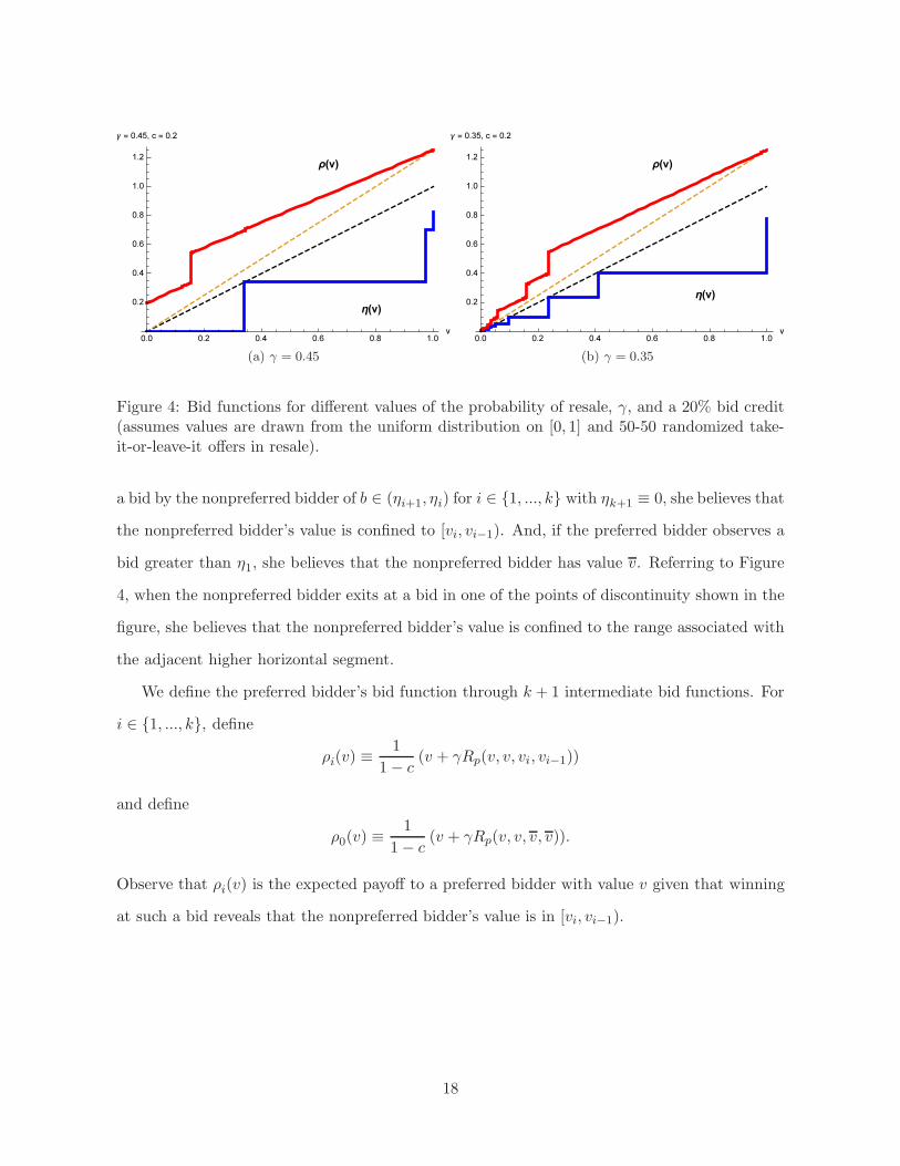
(a) γ = 0.45 (b) γ = 0.35

Figure 4: Bid functions for different values of the probability of resale, γ, and a 20% bid credit(assumes values are drawn from the uniform distribution on [0, 1] and 50-50 randomized take-it-or-leave-it offers in resale).

a bid by the nonpreferred bidder of b ∈ (ηi+1, ηi) for i ∈ {1, ..., k} with ηk+1 ≡ 0, she believes that

the nonpreferred bidder’s value is confined to [vi, vi−1). And, if the preferred bidder observes a

bid greater than η1, she believes that the nonpreferred bidder has value v. Referring to Figure

4, when the nonpreferred bidder exits at a bid in one of the points of discontinuity shown in the

figure, she believes that the nonpreferred bidder’s value is confined to the range associated with

the adjacent higher horizontal segment.

We define the preferred bidder’s bid function through k + 1 intermediate bid functions. For

i ∈ {1, ..., k}, define

ρi(v) ≡1

1− c(v + γRp(v, v, vi, vi−1))

and define

ρ0(v) ≡1

1− c(v + γRp(v, v, v, v)).

Observe that ρi(v) is the expected payoff to a preferred bidder with value v given that winning

at such a bid reveals that the nonpreferred bidder’s value is in [vi, vi−1).

18

The preferred bidder’s bid function is then

ρ(v;v,η) =

ρk(v), if ρk(v) ≤ ηk

ρk−1(v), if ρk(v) > ηk and ρk−1(v) ≤ ηk−1

... ...

ρi−1(v) if ρk(v) > ηk, ..., ρi(v) > ηi, and ρi−1(v) ≤ ηi−1

... ...

ρ0(v), if ρk(v) > ηk, ..., ρ1(v) > η1.

When there is a positive probability of resale, the preferred bidder’s bid function satisfies

ρ(0;v,η) = ρk(0) > 0 and has discontinuities at values v satisfying ρi(v) = ηi for i ∈ {1, ..., k}.

Thus, bids between zero and ρk(0) and between ηi and ρi−1(ρ−1i (ηi)) are off the equilibrium

path, but as described for the case of a one-step equilibrium, regardless of the beliefs held by the

nonpreferred bidder, deviations by the preferred bidder to off-equilibrium bids are not profitable.

A k-step equilibrium exists if there exist v1, ..., vk with 0 < vk < ... < v1 < v and η1, ..., ηk

with 0 < ηk < ... < η1 < argmaxb∈[0,v] π(b; ρ0), which define intermediate bid functions ρ1, ..., ρk,

such that: (i) a nonpreferred bidder with value v is indifferent between bidding η1, and thereby

pooling with nonpreferred bidders with values in [v1, v), and bidding so as to maximize his

expected payoff given that his value is revealed to be v and the preferred bidder bids according

to ρ0; (ii) for any i ∈ {1, ..., k}, a nonpreferred bidder with value vi is indifferent between bidding

ηi, and thereby pooling with nonpreferred bidders with values in [vi, vi−1), and bidding ηi+1,

and thereby pooling with nonpreferred bidders with values in [vi+1, vi).

The equilibrium is defined by 2k parameters, but there are only k+1 equilibrium conditions.

Thus, there are multiple equilibria. We focus on equilibrium with the least number of steps

given the probability of resale.

4 Evaluation of equilibrium outcomes

In order to analyze the effects of resale on welfare in equilibrium, we now consider the specifi-

cation of the resale game with randomized take-it-or-leave-it offers where the preferred bidder

19

makes the offer with probability λ ∈ (0, 1).

The optimal offers in the resale market can be described in terms of the players’ virtual

values and virtual costs. Let Φ(v; b) ≡ v − Fn(b)−Fn(v)fn(v)

be the virtual value of the nonpreferred

bidder whose value v is distributed according to Fn on the support [0, b], with b ∈ [0, v]. Then

the optimal resale offer by the preferred bidder when her value is vp and the bidding has revealed

the nonpreferred bidder’s value to be bounded above by b is t such that Φ(t; b) = vp, which we

denote by Φ−1(vp; b). Similarly, let Γ(v; a) ≡ v +Fp(v)−Fp(a)

fp(v)be the virtual cost of the preferred

bidder whose value is v is distributed according to Fp on the support [a, v], with a ∈ [0, v]. Then

the optimal resale offer by the nonpreferred bidder when his value is vn and the bidding has

revealed the preferred bidder’s value to be bounded below by a is t such that Γ(t; a) = vn, which

we denote by Γ−1(vn; a).20

Social surplus

The auction outcome is ex post efficient when vn ≤ vp because the preferred bidder—who has

the higher value—always wins in those cases. The auction outcome is also ex post efficient when

ρ(vp) < η(vn) because then the nonpreferred bidder has the higher value and the higher bid. In

these cases, there is no scope or need for post-auction transactions. However, when vn > vp and

ρ(vp) ≥ η(vn), the auction outcome is not ex post efficient.

Figure 5 illustrates this for the case of uniformly distributed values and complete obfuscation.

In area A, the preferred bidder has the higher value and wins the auction, giving an efficient

outcome. In area F, the object remains inefficiently with the preferred bidder regardless of

who makes the resale offer. In areas B and C, the preferred bidder has the lower value but

still wins the auction. In area B, the nonpreferred bidder purchases the object in resale with

probability γλ, i.e., only when resale occurs and the preferred bidder makes the offer—when

the nonpreferred bidder makes the offer, he makes an offer below the preferred bidder’s value,

so the offer is rejected. In area C, the nonpreferred bidder purchases the object in resale with

probability γ, i.e., when resale occurs, regardless of who makes the offer. In area E, where

20The virtual value has the interpretation of marginal revenue and that virtual cost that of marginal cost, asfirst observed by Bulow and Roberts (1989), with the probability of trade being interpreted as quantity. Here thevirtual type functions, due to Myerson (1981), are generalized to account for endogenous truncations.

20

vn ≥ Φ−1(vp; v) and vp ≤ Γ−1(vn; 0), the object changes hands in resale only if the nonpreferred

bidder makes the offer, i.e., with probability γ(1− λ).

Figure 5: Welfare with complete obfuscation. Area A: efficient auction outcome; B: efficientoutcome with probability γλ; C: efficient outcome with probability γ; E: efficient outcome withprobability γ(1 − λ); F: inefficient outcome. Curves drawn for the case of c = 0.2 and γ = 0.7,with values drawn from the uniform distribution on [0,1] and 50-50 take-it-or-leave-it offers inresale.

Writing out the expressions for welfare associated with Figure 5, in the case of complete

obfuscation, the expected welfare generated by the auction plus resale conditional on the non-

preferred and preferred bidders’ values is

w(vn, vp) =

vp, if (vn, vp) ∈ A ∪ F

vp + γλ(vn − vp), if (vn, vp) ∈ B

vp + γ(vn − vp), if (vn, vp) ∈ C

vp + γ(1− λ)(vn − vp), if (vn, vp) ∈ E.

When obfuscation is not complete, there is an additional region corresponding to high values

for the nonpreferred bidder and low values for the preferred bidder in which the nonpreferred

bidder efficiently wins the object and there is no resale, generating welfare of vn.

To obtain results on the expected efficiency of outcomes, define W (c, γ) ≡ E [w(vn, vp)].

The direct effect of resale on welfare, which consists of the derivative of W (c, γ) with respect

to γ, not taking into account the effects on η and ρ and how these affect the five regions, is

21

positive. The total effect of resale on welfare also accounts for the effects on η and ρ. However,

in an equilibrium with complete obfuscation the probability of resale does not affect the bidding

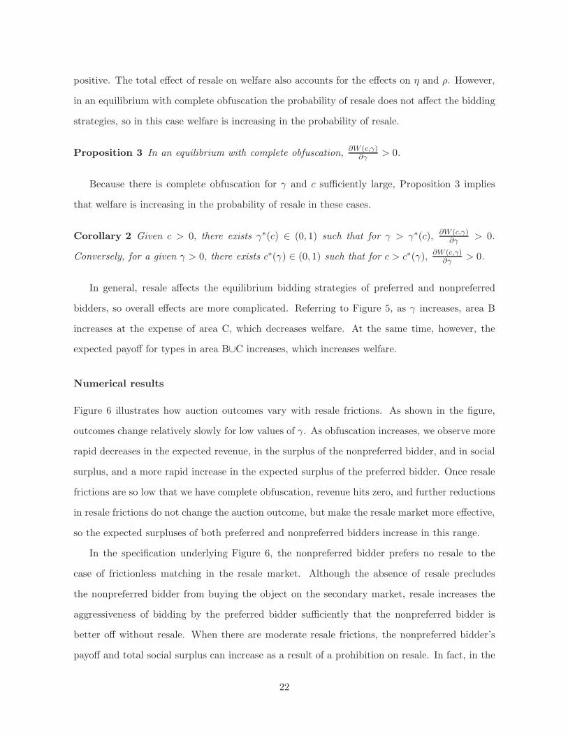
strategies, so in this case welfare is increasing in the probability of resale.

Proposition 3 In an equilibrium with complete obfuscation,∂W (c,γ)

∂γ> 0.

Because there is complete obfuscation for γ and c sufficiently large, Proposition 3 implies

that welfare is increasing in the probability of resale in these cases.

Corollary 2 Given c > 0, there exists γ∗(c) ∈ (0, 1) such that for γ > γ∗(c), ∂W (c,γ)∂γ

> 0.

Conversely, for a given γ > 0, there exists c∗(γ) ∈ (0, 1) such that for c > c∗(γ), ∂W (c,γ)∂γ

> 0.

In general, resale affects the equilibrium bidding strategies of preferred and nonpreferred

bidders, so overall effects are more complicated. Referring to Figure 5, as γ increases, area B

increases at the expense of area C, which decreases welfare. At the same time, however, the

expected payoff for types in area B∪C increases, which increases welfare.

Numerical results

Figure 6 illustrates how auction outcomes vary with resale frictions. As shown in the figure,

outcomes change relatively slowly for low values of γ. As obfuscation increases, we observe more

rapid decreases in the expected revenue, in the surplus of the nonpreferred bidder, and in social

surplus, and a more rapid increase in the expected surplus of the preferred bidder. Once resale

frictions are so low that we have complete obfuscation, revenue hits zero, and further reductions

in resale frictions do not change the auction outcome, but make the resale market more effective,

so the expected surpluses of both preferred and nonpreferred bidders increase in this range.

In the specification underlying Figure 6, the nonpreferred bidder prefers no resale to the

case of frictionless matching in the resale market. Although the absence of resale precludes

the nonpreferred bidder from buying the object on the secondary market, resale increases the

aggressiveness of bidding by the preferred bidder sufficiently that the nonpreferred bidder is

better off without resale. When there are moderate resale frictions, the nonpreferred bidder’s

payoff and total social surplus can increase as a result of a prohibition on resale. In fact, in the

22

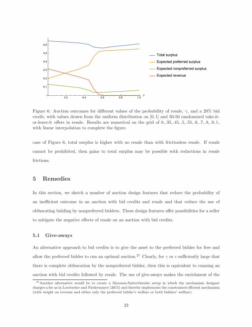
Figure 6: Auction outcomes for different values of the probability of resale, γ, and a 20% bidcredit, with values drawn from the uniform distribution on [0, 1] and 50-50 randomized take-it-or-leave-it offers in resale. Results are numerical on the grid of 0, .35, .45, .5, .55, .6, .7, .8, .9, 1,with linear interpolation to complete the figure.

case of Figure 6, total surplus is higher with no resale than with frictionless resale. If resale

cannot be prohibited, then gains to total surplus may be possible with reductions in resale

frictions.

5 Remedies

In this section, we sketch a number of auction design features that reduce the probability of

an inefficient outcome in an auction with bid credits and resale and that reduce the use of

obfuscating bidding by nonpreferred bidders. These design features offer possibilities for a seller

to mitigate the negative effects of resale on an auction with bid credits.

5.1 Give-aways

An alternative approach to bid credits is to give the asset to the preferred bidder for free and

allow the preferred bidder to run an optimal auction.21 Clearly, for γ or c sufficiently large that

there is complete obfuscation by the nonpreferred bidder, then this is equivalent to running an

auction with bid credits followed by resale. The use of give-aways makes the enrichment of the

21Another alternative would be to create a Myerson-Satterthwaite setup in which the mechanism designercharges a fee as in Loertscher and Niedermayer (2015) and thereby implements the constrained efficient mechanism(with weight on revenue and either only the preferred bidder’s welfare or both bidders’ welfare).

23

preferred bidder painstakingly clear, whereas auctions with bid credits give the appearance of

a more even playing field even though they fail on that dimension when bid credits are large

enough and resale easy enough.

5.2 Reserve prices

The equilibrium bid functions derived above can be adjusted to accommodate a positive reserve.

With a positive reserve, the preferred bidder’s incentive for speculative bidding is reduced be-

cause the preferred bidder needs a sufficiently high value in order to be willing to bid above the

reserve. When the reserve is positive, a nonpreferred bidder with value greater than the reserve

has a reduced incentive for obfuscating bidding because that could result in the object not being

sold at all. Instead the nonpreferred bidder may prefer to pool at a bid equal to the reserve

rather than at a bid of zero.

In the auction with a positive reserve, we assume that the price increases from zero but, even

if only one active bidder remains, does not stop until it reaches the reserve. This is consistent

with the use of reserves in, for example, FCC auctions, where the minimum opening bid is

frequently less than the reserve.

Considering the case with complete obfuscation, the adjustment for a positive reserve involves

defining two cutoff values, vrp for the preferred bidder and vrn for the nonpreferred bidder. With

a positive reserve, the preferred bidder bids below the reserve for values less than vrp, but bids

according to ρ for values greater than vrp. The nonpreferred bidder bids zero for values less than

vrn and bids the reserve for values between vrn and v.

Proposition 4 When there is one preferred bidder and one nonpreferred bidder and there is

complete obfuscation in the absence of a reserve, then the imposition of a reserve r results in an

equilibrium characterized by

ρ(v) =

v, if v < vrp

ρ(v), otherwise,and η(v) =

0, if v < vrn

r, if vrn ≤ v < v

η(v), otherwise,

24

where ρ and η are the equilibrium bid functions in the absence of a reserve and where vrp ∈

[ρ−1(r), (1− c)r] and vrn ≥ 0 are defined by

0 = Ev|Fn

[

vrp − r(1− c) + γRp(vrp, 0, 0, v

rn) | v < vrn

]

(7)

+Ev|Fn

[

vrp − r(1− c) + γRp(vrp, v

rp, v

rn, v) | v

rn ≤ v < v

]

and

γRn(vrn, 0, 0, v

rn) = Ev|Fp

[

vrn − r | v ≤ vrp]

+ γEv|Fp

[

Rn(vrn, v

rp, v

rn, v) | v

rp < v

]

. (8)

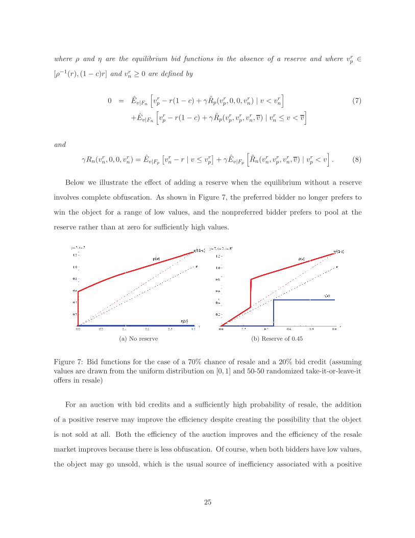
Below we illustrate the effect of adding a reserve when the equilibrium without a reserve

involves complete obfuscation. As shown in Figure 7, the preferred bidder no longer prefers to

win the object for a range of low values, and the nonpreferred bidder prefers to pool at the

reserve rather than at zero for sufficiently high values.

(a) No reserve (b) Reserve of 0.45

Figure 7: Bid functions for the case of a 70% chance of resale and a 20% bid credit (assumingvalues are drawn from the uniform distribution on [0, 1] and 50-50 randomized take-it-or-leave-itoffers in resale)

For an auction with bid credits and a sufficiently high probability of resale, the addition

of a positive reserve may improve the efficiency despite creating the possibility that the object

is not sold at all. Both the efficiency of the auction improves and the efficiency of the resale

market improves because there is less obfuscation. Of course, when both bidders have low values,

the object may go unsold, which is the usual source of inefficiency associated with a positive

25

reserve.22

5.3 Credit caps

Another possibility to limit the effects of bid credits is to impose a cap on the absolute value of

the credit that a bidder may get. For example, the FCC has most recently established a $150

million cap for the dollar value of the credit that a winning preferred bidder can receive.23 Our

model extends easily to allow for such credit caps. Obviously a low cap mitigates or eliminates

the adverse effects of bid credits—in the extreme, a cap of $0 eliminates all effects of bid credits—

but as shown next, large caps do not qualitatively affect our results. In particular, complete

obfuscation can occur in equilibrium when there is resale, rendering credit caps ineffective, even

when the cap is tight enough to improve outcomes without resale. The analysis thus shows that

credit caps may be an effective instrument to limit the adverse effects of bid credits, but it also

emphasizes the importance of accounting for resale markets in the context of auctions with bid

credits.

Consider a cap κ on bid credits, so that the credit received by a preferred bidder who wins

at price b is min{cb, κ}. In the absence of resale, a preferred bidder’s bid function with a cap

is ρ(v) = min{v/(1 − c), v + κ}, so that ρ(v) = v1−c

for v ≤ κ1−cc

and ρ(v) = v + κ otherwise.

Thus, the cap, when it binds, reduces the extent to which the preferred bidder is willing to bid

above her value. A tight cap can reduce overbidding by preferred bidders and underbidding

by nonpreferred bidders, relative to their values, and may prevent complete obfuscation. In

this case, the imposition of the cap increases expected revenue and expected total welfare. It

decreases the expected surplus of the preferred bidder and increases that of the nonpreferred

bidder.

However, a cap that binds in the absence of resale need not have any moderating effect when

resale is possible. For example, consider parameters such that, in the absence of a cap, resale

results in complete obfuscation. If the cap satisfies κ < c1−c

v, then the cap binds in the absence

22For an example in which a positive reserve increases efficiency, for the case of a 20% bid credit and resaleprobability γ = 0.7 (assuming uniform distributions and 50-50 randomized take-it-or-leave-it offers in the resalemarket), an auction with no reserve achieves 89% of maximum welfare, whereas an auction with a reserve ofr = 0.45 does slightly better, achieving 90% of maximum welfare.

23See Section II.B.3 of the FCC’s “Competitive Bidding” Report and Order cited in footnote 8.

26

Figure 8: Bid functions without a cap (ρ and η) and with a cap of κ = 0.1 (ρ and η). The caseshown is for complete obfuscation (γ = 1), where the preferred bidder’s bid function with thecap but with no resale is shown as a thin, solid line. Assumes a 20% bid credit, values that aredrawn from the uniform distribution on [0, 1], and 50-50 randomized take-it-or-leave-it offers inresale.

of resale (which is illustrated as the thin, unbroken line in Figure 8), but the equilibrium with the

cap continues to have complete obfuscation. In the case of complete obfuscation, a nonpreferred

bidder with value v is indifferent between bidding η(v) and zero, and a nonpreferred bidder with

value less than v strictly prefer to bid zero.

For example, as illustrated in Figure 8, for γ sufficiently close to 1, a cap does not affect

the fact that the nonpreferred bidder bids zero whatever his value and that the preferred bidder

bids a positive amount, even when her value is zero, although her maximum bid is altered to

be min{

v1−c

, v + κ}

. Thus, the imposition of such a cap does not change the fact that there is

complete obfuscation in equilibrium. Consequently, the credit cap is ineffective in the presence

of resale even though it improves social surplus (and designer’s revenue) absent resale.

5.4 Anonymous bidding with multiple bidders

We now show how the results of Section 3 adapt to a setting with multiple preferred or non-

preferred bidders. In this setting, a difference arises depending on whether bidders can observe

the exit points of their rivals, so we also discuss the impact of observable versus anonymous

bidding.24

24For example, in the current FCC spectrum license auction format, bidders observe how many other biddersare active, but they do not observe their identities until after the auction is complete, at which time the full

27

To analyze the case of multiple bidders of each kind with observable bidding, we assume

that bidders can exit immediately after one another, so that if one bidder is observed to exit

at a bid of b, then other bidders observing that can also exit at a bid of b, but with the the

order of exits being observable. In the resale game, we assume that a winning preferred bidder

negotiates with the last remaining nonpreferred bidder.

First consider the case of one preferred bidder and multiple nonpreferred bidders. In the

observable bidding case, the nonpreferred bidders remain active up to their values as long as

another nonpreferred bidder is active because exiting when another nonpreferred bidder is active

guarantees a payoff of zero, whereas winning at a bid that is below a bidder’s value generates a

positive payoff.25 If the second-to-last nonpreferred bidder exits at b, then the final nonpreferred

bidder with value v also exits if η(v) < b, and otherwise remains active up to η(v). Thus, there

is pooling by a range of types for the highest-valuing nonpreferred bidder at the value of the

second-highest-valuing nonpreferred bidder. The preferred bidder bids more conservatively than

when facing only one nonpreferred bidder, i.e., according to some ρ(v) ∈(

v1−c

, ρ(v))

, until only

one nonpreferred bidder remains, and then bids up to ρ(v). The more aggressive bidding by the

nonpreferred bidders when multiple nonpreferred bidders are active reduces the expected resale

payoff of the preferred bidder in the event that she wins.

In the case of one nonpreferred bidder and multiple preferred bidders, preferred bidders bid

according to ρ until the last nonpreferred bidder exits. At this point, assuming ρ is a k-step bid

function, the expected resale payoff for a preferred bidder that has value v and wins at a bid of

b such that for some i ∈ {1, ..., k}, η(vi) < b ≤ η(vi−1), is R(v, ρ−1(b), vi−1, vi−2), with v−1 ≡ v.

Thus, following the exit of the last nonpreferred bidder at a bid revealing his value to be in

[vi−1, vi−2), the preferred bidders remain active up to b such that b = v+γR(v,ρ−1(b),vi−1,vi−2)1−c

.

The nonpreferred bidder bids closer to truthfully than he does facing only one preferred bidder,

i.e., according to some η(v) ∈ (η(v), v), until only one preferred bidder remains and then bids

according to η(v). This occurs because the expected payoff to a nonpreferred bidder from resale

history of bids is made public.25In Hu, Kagel, Xu, and Ye (2013), it is also the case that bidding strategies depend on whether another bidder

of the same type remains active. In the model of that paper, two incumbents and a potential entrant competeat an auction, but there is an externality imposed on both incumbents if the entrant wins. In equilibrium, anincumbent has an incentive to exit earlier when the other incumbent is active, free riding on the other incumbent’sincentive to bid so as to exclude the entrant.

28

is lower if multiple preferred bidders remain active.

Anonymous bidding

We assume that under anonymous bidding bidders observe nothing during the auction except

the price. As long as the price continues to increase, active bidders can thus infer that at least

one other bidder is active as well. At the conclusion of the auction, the exit points of all of the

bidders are made public. This means that in the resale game a winning preferred bidder can

identify the highest-bidding nonpreferred bidder.

Given the assumptions just stated, with one preferred and one nonpreferred bidder, equilib-

rium behavior is the same whether bidding is anonymous or not. With one preferred and two

or more nonpreferred bidders, the first-order condition for payoff maximization for the preferred

bidder is the structurally the same (although with a different distribution) as when there is

only one nonpreferred bidder. However, for the nonpreferred bidders, the first-order condition is

different because a nonpreferred bidder must take into account the need to beat the other non-

preferred bidders in order to benefit from resale. This implies that anonymous bidding is closer

to “truthful” in the sense that the preferred bid function is closer to v1−c

and the nonpreferred

bid function is closer to v.

Similarly, anonymous bidding mutes incentives for speculative and counterspeculative bid-

ding when there are multiple bidders of each type. The intuition is that a bidder’s beliefs about

the remaining active bidders will, for certain bid ranges, place positive weight on there being

other bidders of his or her own kind. For example, with multiple preferred bidders, as the bid

increases, there is increasing probability that the bid has increased beyond the exit point of the

last nonpreferred bidder, in which case the expected gains from resale by the winning preferred

bidder decrease. This reduces incentives for speculation. To the extent that anonymity in the

auction reduces the expected value to bidders from resale, this leads to bid functions that are

closer to the bid functions without resale, which increases the expected efficiency of the auction

outcome.26

26Marx (2006) discusses other reasons why anonymous bidding may improve the efficiency of auction outcomesin the context of multiple object auctions.

29

6 Alternative auction formats

The preceding analysis has focused on ascending auctions. In this section, we discuss bid credits

and resale in the context of first and second-price sealed-bid auctions and in the context of

procurement auctions.

6.1 Second-price auctions

The results of Sections 3 and 4 apply equally to second-price sealed bid auctions. However, when

there are multiple preferred and nonpreferred bidders, then the observation of exit by competing

bidders in the open format can be informative about the types of the remaining bidders, and

so differences arise between open ascending and sealed-bid formats. In this case, the second-

price sealed-bid auction corresponds to the case of anonymous bidding in an ascending auction

described in Section 5.

6.2 First-price auctions

In a first-price sealed-bid auction with one preferred and one nonpreferred bidder, letting ρI and

ηI denote preferred and nonpreferred bidders’ first-price bid functions, the preferred bidder’s

problem is

maxb

(v − b(1− c))Prv′|Fn

(

b ≥ ηI(v′))

= maxb

(v − b(1− c))Fn(η−1I (b)).

The first-order condition evaluated at v = ρ−1I (b) is

η−1′I (b) =

(1− c)Fn(η−1I (b))

(ρ−1I (b)− b(1− c))fn(η

−1I (b))

.

The nonpreferred bidder’s problem is

maxb

(v − b)Prv′|Fp

(

b ≥ ρI(v′))

= maxb

(v − b)Fp(ρ−1I (b)),

30

This first-order condition evaluated at v = η−1I (b) is

ρ−1′I (b) =

Fρ(ρ−1I (b))

(η−1I (b)− b)fp(ρ

−1I (b))

.

We can redefine the preferred bidder’s value as v = v1−c

, where v is drawn from the distribution

Fp(v) = Fp(v(1− c)) with support [0, v1−c

]. Then we have bid functions defined by

η−1′(b) =Fn(η

−1(b))

(ρ−1(b)− b)fn(η−1(b))

and ρ−1′(b) =Fp(ρ

−1(b))

(η−1(b)− b)fp(ρ−1(b))

,

which is equivalent to an asymmetric first-price auction problem with no bid credit and bidders

drawing from Fn and Fp as analyzed by Hafalir and Krishna (2008).

The expected revenue in a first-price auction with bid credit c is equal to the expected

revenue from the transformed auction, where the preferred bidder draws from Fp, with no bid

credit, minus the additional term c∫ v

0

∫ v

ρ−1

I(ηI(vn))

ρ(vp)dFp(vp)dFn(vn).

6.3 Procurement auctions

Bid credits are widely used in procurement auctions. In this subsection, we briefly explain how

the results from the preceding analysis carry over to this important setup, with minimal and

obvious adjustments.

Descending procurement auctions

The results of Section 3 can be restated for the case of a procurement organized as a descending

auction. If a bid credit takes the form of a percentage increase in the payment made to a preferred

bidder who has the lowest bid, and if subcontracting is possible, then preferred bidders have

an incentive to shade their bids downward and nonpreferred bidders have an incentive to shade

their bids upward.

Thus, when subcontracting is possible, bid credits lead to inefficiencies whereby a preferred

bidder may win the procurement auction even though she does not have the lowest cost. The

winning preferred bidder has an incentive to subcontract to a lower cost bidder, profiting from

the markup to the procurer. To the extent that the procurer values having production performed

31

by a preferred bidder, the incentive to take advantage of the bid credit and then subcontract

can reduce the benefits of a bid credit program.

First-price sealed-bid procurement auctions

Similar results apply to first-price sealed-bid procurement auctions. In that case, assuming one

preferred and one nonpreferred bidder with costs drawn from Fp and Fn, respectively, expected

profit for a preferred bidder with cost v when the preferred bidder bids bp and the nonpreferred

bidder bids bn is πp(v) = (bp − v) Prbn (bp ≤ (1 + c)bn). Her first-order condition is thus

η−1′ (b) =1− Fn

(

η−1 (b))

(b(1 + c)− ρ−1((1 + c)b)) fn (η−1 (b))(1 + c).

The nonpreferred bidder with cost v has expected profit πn(v) = (bn−v) Prbp (bp ≥ (1 + c)bn).Consequently,

his first-order condition is

ρ−1′(b) =1− Fp

(

ρ−1(b))

fp (ρ−1(b))(

b1+c

− η−1( b1+c

))

1

1 + c.

Given initial conditions, one can then define the equilibrium bid functions.27

7 Conclusion

Bid credits are widely used in auctions and procurements. Favouring some bidders over others,

bid credits induce inefficient auction outcomes with positive probability, which creates scope

and pressure for post-auction resale or, in the procurement context, for subcontracting. Al-

though such post-auction transactions unambiguously improve social outcomes if they are not

anticipated by bidders in the auction, our equilibrium analysis shows that when post-auction

transactions are anticipated by bidders, auction outcomes are made unambiguously less efficient.

Because the prospect of post-auction transactions increases the value of winning for the

27For initial conditions, assume a preferred bidder with the highest possible cost v bids b to maximize

(b − v)(

1− Fn

(

b1+c

))

, which implies 1

b−v=

fn

(

b

1+c

)

11+c

1−Fn

(

b

1+c

) . A nonpreferred bidder cost v ∈ [ b1+c

, v] has a zero

probability of winning and, therefore, bids his cost. There exists a bid level b such that ρ(v) = b. For thenonpreferred bidder with lowest possible cost v, η(v) = b/(1 + c).

32

preferred bidder and the value of losing for the nonpreferred bidder, the possibility of resale

or subcontracting induces speculative and counterspeculative bidding by the preferred and the

nonpreferred bidder. This makes the auction less efficient and means that the prospect of

post-auction transactions reinforces the desirability of such transactions. Moreover, because the

counterspeculative bid shading by the nonpreferred bidder is more likely to obfuscate his value

the higher is the probability that the resale market operates, an increase in the probability that

the resale market operates can decrease of the total surplus that is generated from the auction

and the resale market. Thus, the prospect of post-auction transactions makes such transactions

more desirable to correct inefficient auction outcomes but less effective at doing so because of

obfuscation.

We analyze a number of remedies that may mitigate the inefficiencies associated with bid

credits and resale or subcontracting. One possible remedy is the imposition of caps on the

absolute dollar amount a preferred bidder may be credited for. As a case in point, such caps

have recently been introduced by the FCC. Our analysis reveals that such caps unambiguously

improve outcomes without resale or subcontracting, provided they bind some of the time. If

chosen tight enough, they also do so with resale and subcontracting. However, even if a cap

improves outcomes without the possibility of post-auction transactions, the same cap may be

completely ineffective with resale or subcontracting if it is not tight enough to overcome complete

obfuscation.

Throughout the paper, we have maintained the view that bid credits are exogenously im-

posed, hindering the socially efficient allocation of resources. This is arguably an appropriate

perspective in some instances and circumstances. However, it is also plausible and possible that

bid credits are imposed to achieve desirable social goals such as inducing a competitive market

structure downstream. When viewed from this angle, our paper provides the first step toward an

integrated analysis of optimal bid credits by analyzing the subgame that ensues after bid credits

have been determined. Analyzing the full game, for which our paper delivers the equilibrium

analysis for the second stage, seems an excellent avenue for future research.

33

A Appendix: Resale with randomized take-it-or-leave-it offers

In this appendix, we formulate resale payoffs assuming randomized take-it-or-leave-it offers.

Bidders in our model with one preferred and one nonpreferred bidder update their beliefs about

the value of other bidder based on the observed bidding. Thus, we define the optimal resale

offers given updated beliefs. When resale is possible and the preferred bidder wins, we assume

that the preferred bidder makes the offer with probability λ and the nonpreferred bidder makes

the offer with probability 1− λ.

Define virtual value Φ and virtual cost Γ as in Section 4. If a preferred bidder with value

v makes an offer to sell the object to a nonpreferred bidder when the nonpreferred bidder is

believed to have a value in [a, b], then the optimal resale offer is

op(v, a, b) ≡

max{v, a,Φ−1(v; b)}, if a < b

b, if a = b and v < a

v, if a = b and v ≥ a.

Similarly, the optimal purchase offer by a nonpreferred bidder with value v to a preferred bidder,

conditional on the preferred bidder’s value being in [a, b], is

on(v, a, b) ≡

min{

v, b,Γ−1(v; a)}

, if a < b

a, if a = b and v < a

0, if a = b and v ≥ a.

The net benefit to the preferred bidder with value v from resale to a nonpreferred bidder

when the bidding indicates the lower bound on the preferred bidder’s value is v, conditional on

the nonpreferred bidder’s value being in [ℓ, h] , is

Rp(v, v, ℓ, h) = λmax {0, op(v, ℓ, h) − v}1

Prv′|Fn(v′ ∈ [ℓ, h])

+(1− λ)Ev′|Fn

[

max{

0, on(v′, v, v)− v

}

| v′ ∈ [ℓ, h]]

.

The net benefit to a nonpreferred bidder with value v from a resale purchase from a preferred

34

bidder when the bidding indicates that the nonpreferred bidder’s value is in [ℓ, h] , conditional

on the preferred bidder’s value being greater than v, is

Rn(v, v, ℓ, h) = λEv′|Fp

[

max{0, v − op(v′, ℓ, h)} | v < v′

]

+(1− λ)max {0, vn − on (v, v, v)}Prv′|Fp

(

v′ < on (v, v, v) | v < v′)

.

B Appendix: Uniformly distributed values

In this appendix, for the case in which values are drawn from the uniform distribution on [0, 1],

we provide expressions for preferred and nonpreferred expected resale payoffs, the optimal bid of

a nonpreferred bidder with value v, and the threshold resale probability for complete obfuscation.

Resale payoffs

In the uniform case, we can write the resale payoffs when resale takes the form of randomized

take-it-or-leave-it offers, as defined in Appendix A, as follows. For v > v and ℓ ≤ h,

Rn(v, v, ℓ, h) = λ1

1− v

∫ v

v

max

{

0, v −max

{

ℓ,vp + h

2

}}

dvp + (1− λ)

(

v − v

2

)2 1

1− v,

for v < h and ℓ < h,

Rp(v, v, ℓ, h) = λ

(

max

{

ℓ,v + h

2

}

− v

)

h−max{

ℓ, v+h2

}

h− ℓ+(1−λ)

1

h− ℓ

∫ h

ℓ

max

{

0,vn + v

2− v

}

dvn,

and v < h,

Rp(v, v, h, h) = λ (h− v) + (1− λ)max

{

0,h+ v

2− v

}

.

It follows that

Rn(v, ρ−1(b), v, v) = (1− λ)

(

v − ρ−1(b)

2

)21

1− ρ−1(b). (9)

35

Optimal bid of a nonpreferred bidder with value v

For the uniform case, we can write (3) as:

π(b; ρ) =

∫ ρ−1(b)

0(v − ρ(vp))dvp + γ(1− ρ−1(b))Rn(v, ρ

−1(b), v, v),

with v = 1. Using (9) and taking the derivative,

dπ(b; ρ)

db= ρ−1′(b)(v − b)− γ(1− λ)

v − ρ−1(b)

2ρ−1′(b),

so the first-order condition for the optimal bid, dπ(b;ρ)db

∣

∣

∣

b=b= 0, implies v− b = γ(1−λ)v−ρ−1(b)

2 .

Substituting in for ρ−1(b), we have b = v 1−γ

1−γ(1+λ)−γ(1−λ) 12(1−c)

.

Threshold resale probability for complete obfuscation

For the uniform case, the expected payoff from complete obfuscation given by the right side of

(4) is

γRn(v, 0, 0, v) = γλ

∫ v

0

(

v −vp + v

2

)

dvp + γ(1− λ)v2

4= γ

v2

4.

Thus, the requirement condition for existence of an equilibrium with complete obfuscation is

γ ≥4∫ ρ−1(b)0 (v − ρ(vp))dvp

λv2 + (1− λ)2vρ−1(b)− (1− λ)ρ−1(b)2,

where b maximizes π0n. The cutoff value of γ is approximately 0.6.

C Appendix: Proofs

Proof of Proposition 4. Taking as given the strategy of the nonpreferred bidder, the expected

payoff to a preferred bidder with value vp from bidding ρ(vp) > r is given by the right side of (7).

As shown in that expression, the preferred bidder wins and pays r(1−c) if vn < η−1(r), where vn

is the nonpreferred bidder’s value, and otherwise wins when η(vn) < ρ(vp) and pays η(vn)(1−c).

The bidding reveals whether vn is in [0, vrn), [vrn, η

−1(r)), or reveals vn for vn > η−1(r). Equation

(7) says that a preferred bidder with value vrp is indifferent between bidding vrp/(1− c), which is

36

less than r and loses with probability one, and bidding ρ(vrp), which is greater than r.

Taking as given the strategy of the preferred bidder, the expected payoff from a nonpreferred

bidder with value vrn from bidding zero is Rn(vrn, 0, 0, v

rn) because the bidder learns nothing about

the preferred bidder’s value and reveals that his value is bounded above by vrn. The expected

payoff of a nonpreferred bidder with value vrn from bidding r is given by the right side of (8),

where the first term occurs because the nonpreferred bidder wins at a price of r if vp < vrp, and

the second term reflects the nonpreferred bidder’s expected payoff from resale when the preferred

bidder wins, i.e., vp > vrp, with the bidding revealing that vp > vrp and that the nonpreferred

bidder’s value is less than η−1(r). Thus, equation (8) says that a nonpreferred bidder with value

vrn is indifferent between bidding zero and bidding r. One can show that equations (7) an (8)

define vrp ∈ [ρ−1(r), (1− c)r] and vrn ∈ [0, v].

The result that it is a best response for a nonpreferred bidder with value v greater than

η−1(r) to bid η(v) follows from η being a best response in an environment with no reserve.

Q.E.D.

37

References

Argitis, T., and C. Pellegrini (2014): “Canada Sets Aside More Spectrum for Small Wire-

less Firms,” Bloomberg News, July 7, 2014.

Athey, S., D. Coey, and J. Levin (2013): “Set-Asides and Subsidies in Auctions,” American

Economic Journal: Microeconomics, 5(1), 1–27.

Ausubel, L., and P. Cramton (2004): “Auctioning Many Divisible Goods,” Journal of the

European Economic Association, 2(2-3), 480–493.

Brannman, L., and L. M. Froeb (2000): “Mergers, Cartels, Set-Asides, and Bidding Prefer-

ences in Asymmetric Oral Auctions,” Review of Economics and Statistics, 82(2), 283–290.

Bulow, J., and J. Roberts (1989): “The Simple Economics of Optimal Auctions,” Journal

of Political Economics, 97(5), 1060–90.

Denes, T. A. (1997): “Do Small Business Set-Asides Increase the Cost of Government Con-

tracting?,” Public Administration Review, 57(5), 441–444.

Garratt, R., and T. Troger (2006): “Speculation in Standard Auctions with Resale,”

Econometrica, 74(3), 753–769.

Garratt, R. J., T. Troger, and C. Z. Zheng (2009): “Collusion via Resale,” Econometrica,

77(4), 1095–1136.

Gupta, M., and B. Lebrun (1999): “First Price Auctions with Resale,” Economics Letters,

64(2), 181–185.

Hafalir, I., and V. Krishna (2008): “Asymmetric Auctions with Resale,” American Eco-

nomic Review, 98(1), 87–112.

Hafalir, I., and V. Krishna (2009): “Revenue and Efficiency Effects of Resale in First-Price

Auctions,” Journal of Mathematical Economics, 45, 589–602.

Haile, P. A. (2003): “Auctions with Private Uncertainty and Resale Opportunities,” Journal

of Economic Theory, 108(1), 72–110.

38

Harrington, Joseph E., J. (1986): “Limit Pricing when the Potential Entrant is Uncertain

of its Cost Function,” Econometrica, 54(2), 429–437.

Hu, Y., J. Kagel, X. Xu, and L. Ye (2013): “Optimal Nonparametric Estimation of First-

Price Auctions,” Theoretical and Experimental Analysis of Auctions with Negative Externali-

ties, 82, 269–291.

Krasnokutskaya, E., and K. Seim (2011): “Bid Preference Programs and Participation in

Highway Procurement Auctions,” American Economic Review, 101(6), 2653–2686.

Lebrun, B. (2010a): “First-Price Auctions with Resale and with Outcomes Robust to Bid

Disclosure,” RAND Journal of Economics, 41(1), 165–178.

(2010b): “Revenue Ranking of First-Price Auctions with Resale,” Journal of Economic

Theory, 145, 2037–2043.

(2012): “Optimality and the English and Second-Price Auctions with Resale,” Games

and Economic Behavior,, 75(2), 731–751.

Loertscher, S., and A. Niedermayer (2015): “Percentage Fees in Thin Markets: An Opti-

mal Pricing Perspective,” Mimeo, University of Mannheim and University of Melbourne.

Marion, J. (2007): “Are Bid Preferences Benign? The Effect of Sbusiness Subsidies in Highway

Procurement Auctions,” Journal of Public Economics, 91(7–8), 1591–1624.

(2009): “How Costly Is Affirmative Action? Government Contracting and California’s

Proposition 209,” Review of Economics and Statistics, 91(3), 503–522.

Marx, L. M. (2006): “Economics at the Federal Communications Commission,” Review of

Industrial Organization, 29, 349–368.

McAfee, R. P., J. McMillan, and P. J. Reny (1989): “Extracting the Surplus in the

Common-Value Auction.,” Econometrica, 57(6), 1451–1459.

Milgrom, P., and R. Weber (1982): “A Theory of Auctions and Competitive Bidding,”

Econometrica, 50, 1089–1122.

39

Myerson, R. B. (1981): “Optimal Auction Design,” Mathematical Operations Research, 6(1),

58–73.

National Association of State Procurement Officials (2012): “2011-2012

NASPO Survey of State Procurement Practices Summary Report,” available at

http://naspo.org/survey/Documents/ Zip/FINAL SummaryReport 2011-2012 Survey 6-28-

12.pdf, accessed October 27, 2014.

Pagnozzi, M. (2007): “Bidding to Lose? Auctions with Resale,” RAND Journal of Economics,

38(4), 1090–1112.

(2010): “Are Speculators Unwelcome in Multi-Object Auctions?,” American Economic

Journal: Microeconomics, 2(2), 97–131.

Pagnozzi, M., and K. J. Saral (2016): “Entry by Successful Speculators in Auctions with

Resale,” Working Paper, University of Naples Federico II.

(forthcoming): “Demand Reduction in Multi-Object Auctions with Resale: An Exper-

imental Analysis,,” Economic Journal.

Pai, M. M., and R. Vohra (2012): “Auction Design with Fairness Concerns: Subsidies vs. Set-

Asides,” Discussion Paper, Center for Mathematical Studies in Economics and Management

Science, Northwestern University.

Virginia Department of General Services – Division of Purchases and Sup-

ply (2010): “Listing of States’ Absolute and Percentage Preferences,” available at

http://www.ilsr.org/wp-content/uploads/2008/12/listing-states-preferences.pdf, accessed Oc-

tober 27, 2014.

Wilson, R. (1993): Nonlinear Pricing. Oxford University Press.

Xu, X., D. Levin, and L. Ye (2013): “Auctions with Entry and Resale,” Games and Economic

Behavior, 72, 92–105.

Zhang, J., and R. Wang (2013): “Optimal Mechanism Design with Resale Via Bargaining,”

Journal of Economic Theory, 148, 2096–2123.

40

Zheng, C. Z. (2002): “Optimal Auction with Resale,” Econometrica, 70(6), 2197–2224.

41