lm · 2019-04-05 · 1/13/19 6 google n-gram release •serve as the incoming 92 •serve as the...

1/13/19

1

CS 6120/CS 4120: Natural Language Processing

Instructor: Prof. Lu WangCollege of Computer and Information Science

Northeastern UniversityWebpage: www.ccs.neu.edu/home/luwang

Updated Office Hours

• Prof. Lu Wang, Fridays 3pm - 4pm, or by appointment, Rm 911, 177 Huntington Ave.• TA Ruiyang Xu (email: [email protected]), Mondays 4pm-5pm, or by

appointment, 132H Nightingale• TA Nikhil Badugu (email: [email protected]), Wednesdays 3:30pm-

4:30pm, or by appointment, 132H Nightingale• TA Parmeet Singh Saluja (email: [email protected]), Thursdays 5pm-6pm,

or by appointment, 132H Nightingale

• Course Website:• http://www.ccs.neu.edu/home/luwang/courses/cs6120_sp2019/cs6120_sp2019.

html

Outline

• Probabilistic language model and n-grams

• Estimating n-gram probabilities• Language model evaluation and perplexity

• Generalization and zeros• Smoothing: add-one

• Interpolation, backoff, and web-scale LMs• Smoothing: Kneser-Ney Smoothing

[Modified from Dan Jurafsky’s slides]

Probabilistic Language Models

•Assign a probability to a sentence•Machine Translation:• P(high winds tonight) > P(large winds tonight)

•Spell Correction• The office is about fifteen minuets from my house• P(about fifteen minutes from) > P(about fifteen minuets from)

•Speech Recognition• P(I saw a van) >> P(eyes awe of an)

•Text Generation in general: • Summarization, question-answering …

Probabilistic Language Modeling

• Goal: compute the probability of a sentence or sequence of words:P(W) = P(w1,w2,w3,w4,w5…wn)

• Related task: probability of an upcoming word:P(w5|w1,w2,w3,w4)

• A model that computes either of these:P(W) or P(wn|w1,w2…wn-1) is called a language model.

• Better: the grammar • But language model (or LM) is standard

How to compute P(W)

• How to compute this joint probability:

•P(its, water, is, so, transparent, that)

http://www.ccs.neu.edu/home/luwang

http://www.ccs.neu.edu/home/luwang/courses/cs6120_sp2019/cs6120_sp2019.html

1/13/19

2

How to compute P(W)

• How to compute this joint probability:

•P(its, water, is, so, transparent, that)

• Intuition: let’s rely on the Chain Rule of Probability

Quick Review: Probability

• Recall the definition of conditional probabilities

p(B|A) = P(A,B)/P(A) Rewriting: P(A,B) = P(A)P(B|A)

• More variables:

P(A,B,C,D) = P(A)P(B|A)P(C|A,B)P(D|A,B,C)

• The Chain Rule in General

P(x1,x2,x3,…,xn) = P(x1)P(x2|x1)P(x3|x1,x2)…P(xn|x1,…,xn-1)

The Chain Rule applied to compute joint probability of words in sentence

€

P(w1w2…wn ) = P(wi |w1w2…wi−1)i∏

The Chain Rule applied to compute joint probability of words in sentence

P(“its water is so transparent”) =P(its) × P(water|its) × P(is|its water)

× P(so|its water is) × P(transparent|its water is so)

€

P(w1w2…wn ) = P(wi |w1w2…wi−1)i∏

How to estimate these probabilities

• Could we just count and divide?

€

P(the | its water is so transparent that) =

Count(its water is so transparent that the)Count(its water is so transparent that)

How to estimate these probabilities

• Could we just count and divide?

• No! Too many possible sentences!•We’ll never see enough data for estimating these

€

P(the | its water is so transparent that) =

Count(its water is so transparent that the)Count(its water is so transparent that)

1/13/19

3

Markov Assumption

•Simplifying assumption:

•Or maybe

€

P(the | its water is so transparent that) ≈ P(the | that)

€

P(the | its water is so transparent that) ≈ P(the | transparent that)

Markov Assumption

•In other words, we approximate each component in the product

€

P(w1w2…wn ) ≈ P(wi |wi−k…wi−1)i∏

€

P(wi |w1w2…wi−1) ≈ P(wi |wi−k…wi−1)

Simplest case: Unigram model

fifth, an, of, futures, the, an, incorporated, a, a, the, inflation, most, dollars, quarter, in, is, mass

thrift, did, eighty, said, hard, 'm, july, bullish

that, or, limited, the

Some automatically generated sentences from a unigram model

€

P(w1w2…wn ) ≈ P(wi)i∏ Condition on the previous word:

Bigram model

texaco, rose, one, in, this, issue, is, pursuing, growth, in, a, boiler, house, said, mr., gurria, mexico, 's, motion, control, proposal, without, permission, from, five, hundred, fifty, five, yen

outside, new, car, parking, lot, of, the, agreement, reached

this, would, be, a, record, november

€

P(wi |w1w2…wi−1) ≈ P(wi |wi−1)

N-gram models

•We can extend to trigrams, 4-grams, 5-grams

N-gram models

•We can extend to trigrams, 4-grams, 5-grams• In general this is an insufficient model of language• because language has long-distance dependencies:

“The computer(s) which I had just put into the machine room on the fifth floor is (are) crashing.”

•But we can often get away with N-gram models

1/13/19

4

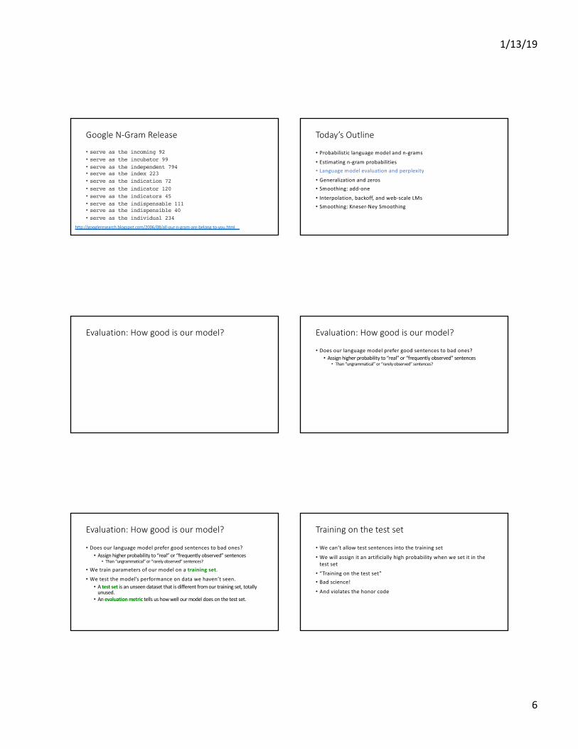
Today’s Outline

• Probabilistic language model and n-grams• Estimating n-gram probabilities• Language model evaluation and perplexity• Generalization and zeros• Smoothing: add-one• Interpolation, backoff, and web-scale LMs• Smoothing: Kneser-Ney Smoothing

Estimating bigram probabilities

• The Maximum Likelihood Estimate for bigram probability

€

P(wi |wi−1) =count(wi−1,wi)count(wi−1)

€

P(wi |wi−1) =c(wi−1,wi)c(wi−1)

An example

<s> I am Sam </s><s> Sam I am </s><s> I do not like green eggs and ham </s>

€


An example

<s> I am Sam </s><s> Sam I am </s><s> I do not like green eggs and ham </s>

€


More examples: Berkeley Restaurant Project sentences

• can you tell me about any good cantonese restaurants close by•mid priced thai food is what i’m looking for• tell me about chez panisse• can you give me a listing of the kinds of food that are available• i’m looking for a good place to eat breakfast•when is caffe venezia open during the day

Raw bigram counts

• Out of 9222 sentences

1/13/19

5

Raw bigram probabilities

• Normalize by unigrams:

• Result:

Bigram estimates of sentence probabilities

P(<s> I want english food </s>) =P(I|<s>) × P(want|I) × P(english|want) × P(food|english) × P(</s>|food)

= .000031

Knowledge

•P(english|want) = .0011•P(chinese|want) = .0065•P(to|want) = .66•P(eat | to) = .28•P(food | to) = 0•P(want | spend) = 0•P (i | <s>) = .25

Practical Issues

•We do everything in log space•Avoid underflow•(also adding is faster than multiplying)

log(p1 × p2 × p3 × p4 ) = log p1 + log p2 + log p3 + log p4

Language Modeling Toolkits

•SRILM•http://www.speech.sri.com/projects/srilm/

Google N-Gram Release, August 2006

…

http://www.speech.sri.com/projects/srilm/

1/13/19

6

Google N-Gram Release

• serve as the incoming 92• serve as the incubator 99• serve as the independent 794• serve as the index 223• serve as the indication 72• serve as the indicator 120• serve as the indicators 45• serve as the indispensable 111• serve as the indispensible 40• serve as the individual 234

http://googleresearch.blogspot.com/2006/08/all-our-n-gram-are-belong-to-you.html

Today’s Outline


Evaluation: How good is our model? Evaluation: How good is our model?

• Does our language model prefer good sentences to bad ones?• Assign higher probability to “real” or “frequently observed” sentences

• Than “ungrammatical” or “rarely observed” sentences?

Evaluation: How good is our model?

• Does our language model prefer good sentences to bad ones?• Assign higher probability to “real” or “frequently observed” sentences

• Than “ungrammatical” or “rarely observed” sentences?

• We train parameters of our model on a training set.• We test the model’s performance on data we haven’t seen.• A test set is an unseen dataset that is different from our training set, totally

unused.• An evaluation metric tells us how well our model does on the test set.

Training on the test set

• We can’t allow test sentences into the training set• We will assign it an artificially high probability when we set it in the

test set• “Training on the test set”• Bad science!• And violates the honor code

http://googleresearch.blogspot.com/2006/08/all-our-n-gram-are-belong-to-you.html

1/13/19

7

Extrinsic evaluation of N-gram models

•Best evaluation for comparing models A and B• Put each model in a task• spelling corrector, speech recognizer, MT system

• Run the task, get an accuracy for A and for B• How many misspelled words corrected properly• How many words translated correctly

• Compare accuracy for A and B

Difficulty of extrinsic evaluation of N-gram models•Extrinsic evaluation• Time-consuming; can take days or weeks

•So• Sometimes use intrinsic evaluation: perplexity

Difficulty of extrinsic evaluation of N-gram models•Extrinsic evaluation• Time-consuming; can take days or weeks

•So• Sometimes use intrinsic evaluation: perplexity• Bad approximation • unless the test data looks just like the training data• So generally only useful in pilot experiments

• But is helpful to think about.

Intuition of Perplexity

• The Shannon Game:• How well can we predict the next word?

• Unigrams are terrible at this game. (Why?)• A better model of a text• is one which assigns a higher probability to the word that actually occurs

I always order pizza with cheese and ____

The 33rd President of the US was ____

I saw a ____

Intuition of Perplexity

• The Shannon Game:• How well can we predict the next word?

• Unigrams are terrible at this game. (Why?)• A better model of a text

• is one which assigns a higher probability to the word that actually occurs

I always order pizza with cheese and ____

The 33rd President of the US was ____I saw a ____

mushrooms 0.1

pepperoni 0.1

anchovies 0.01

….

fried rice 0.0001

….

and 1e-100

Perplexity

Perplexity is the inverse probability of the test set, normalized by the number of words:

The best language model is one that best predicts an unseen test set• Gives the highest P(sentence)

PP(W ) = P(w1w2...wN )−

1N

=1

P(w1w2...wN )N

1/13/19

8

Perplexity


Chain rule:

For bigrams:


PP(W ) = P(w1w2...wN )−

1N

=1

P(w1w2...wN )N

Perplexity


Chain rule:

For bigrams:

Minimizing perplexity is the same as maximizing probability


PP(W ) = P(w1w2...wN )−

1N

=1

P(w1w2...wN )N

Perplexity as branching factor

• Let’s suppose a sentence consisting of random digits• What is the perplexity of this sentence according to a model that

assign P=1/10 to each digit?

Perplexity as branching factor

• Let’s suppose a sentence consisting of random digits• What is the perplexity of this sentence according to a model that

assign P=1/10 to each digit?

Lower perplexity = better model

•Training 38 million words, test 1.5 million words, WSJ

N-gram Order

Unigram Bigram Trigram

Perplexity 962 170 109

Today’s Outline


1/13/19

9

The perils of overfitting

•N-grams only work well for word prediction if the test corpus looks like the training corpus• In real life, it often doesn’t•We need to train robust models that generalize!

The perils of overfitting

•N-grams only work well for word prediction if the test corpus looks like the training corpus• In real life, it often doesn’t•We need to train robust models that generalize!•One kind of generalization: Zeros!•Things that don’t ever occur in the training set•But occur in the test set

Zeros

In training set, we see… denied the allegations… denied the reports… denied the claims… denied the request

P(“offer” | denied the) = 0

But in test set,… denied the offer… denied the loan

Zero probability bigrams

• Bigrams with zero probability• mean that we will assign 0 probability to the test set!

• And hence we cannot compute perplexity (can’t divide by 0)!

Today’s Outline


The intuition of smoothing (from Dan Klein)

• When we have sparse statistics:

• Steal probability mass to generalize better

P(w | denied the)3 allegations2 reports1 claims1 request7 total

P(w | denied the)2.5 allegations1.5 reports0.5 claims0.5 request2 other7 total

alle

gatio

ns

repo

rts

clai

ms

atta

ck

requ

est

man

outc

ome

…

alle

gatio

ns

atta

ck

man

outc

ome

…alle

gatio

ns

repo

rts

claim

s

requ

est

1/13/19

10

Add-one estimation

•Also called Laplace smoothing• Pretend we saw each word one more time than we did• Just add one to all the counts! (Instead of taking away

counts)

•MLE estimate:

•Add-1 estimate:

PMLE (wi |wi−1) =c(wi−1,wi )c(wi−1)

PAdd−1(wi |wi−1) =c(wi−1,wi )+1c(wi−1)+V

V is the size of vocabulary

Add-one estimation

•Also called Laplace smoothing• Pretend we saw each word one more time than we did• Just add one to all the counts! (Instead of taking away

counts)

•MLE estimate:

•Add-1 estimate:

PMLE (wi |wi−1) =c(wi−1,wi )c(wi−1)

PAdd−1(wi |wi−1) =c(wi−1,wi )+1c(wi−1)+V Why add V?

Berkeley Restaurant Corpus: Laplace smoothed bigram counts

Laplace-smoothed bigrams

Add-1 estimation is a blunt instrument

• So add-1 isn’t used for N-grams: • We’ll see better methods • (nowadays, neural LM becomes popular, will discuss later)

• But add-1 is used to smooth other NLP models• For text classification (coming soon!) • In domains where the number of zeros isn’t so huge.

• Add-1 can be extended to add-k (k can be any positive real number)

Today’s Outline


1/13/19

11

Backoff and Interpolation• Sometimes it helps to use less context• Condition on less context for contexts you haven’t learned much about

• Backoff: • use trigram if you have good evidence• otherwise bigram• otherwise unigram

• Interpolation: • mix unigram, bigram, trigram

• In general, interpolation works better

Linear Interpolation

•Simple interpolation

4.4 • SMOOTHING 15

The sharp change in counts and probabilities occurs because too much probabil-ity mass is moved to all the zeros.

4.4.2 Add-k smoothing

One alternative to add-one smoothing is to move a bit less of the probability massfrom the seen to the unseen events. Instead of adding 1 to each count, we add a frac-tional count k (.5? .05? .01?). This algorithm is therefore called add-k smoothing.add-k

P⇤Add-k(wn|wn�1) =

C(wn�1wn)+ kC(wn�1)+ kV

(4.23)

Add-k smoothing requires that we have a method for choosing k; this can bedone, for example, by optimizing on a devset. Although add-k is is useful for sometasks (including text classification), it turns out that it still doesn’t work well forlanguage modeling, generating counts with poor variances and often inappropriatediscounts (Gale and Church, 1994).

4.4.3 Backoff and Interpolation

The discounting we have been discussing so far can help solve the problem of zerofrequency N-grams. But there is an additional source of knowledge we can drawon. If we are trying to compute P(wn|wn�2wn�1) but we have no examples of aparticular trigram wn�2wn�1wn, we can instead estimate its probability by usingthe bigram probability P(wn|wn�1). Similarly, if we don’t have counts to computeP(wn|wn�1), we can look to the unigram P(wn).

In other words, sometimes using less context is a good thing, helping to general-ize more for contexts that the model hasn’t learned much about. There are two waysto use this N-gram “hierarchy”. In backoff, we use the trigram if the evidence isbackoff

sufficient, otherwise we use the bigram, otherwise the unigram. In other words, weonly “back off” to a lower-order N-gram if we have zero evidence for a higher-orderN-gram. By contrast, in interpolation, we always mix the probability estimatesinterpolation

from all the N-gram estimators, weighing and combining the trigram, bigram, andunigram counts.

In simple linear interpolation, we combine different order N-grams by linearlyinterpolating all the models. Thus, we estimate the trigram probability P(wn|wn�2wn�1)by mixing together the unigram, bigram, and trigram probabilities, each weightedby a l :

P̂(wn|wn�2wn�1) = l1P(wn|wn�2wn�1)

+l2P(wn|wn�1)

+l3P(wn) (4.24)

such that the l s sum to 1: X

i

li = 1 (4.25)

In a slightly more sophisticated version of linear interpolation, each l weight iscomputed in a more sophisticated way, by conditioning on the context. This way,if we have particularly accurate counts for a particular bigram, we assume that thecounts of the trigrams based on this bigram will be more trustworthy, so we canmake the l s for those trigrams higher and thus give that trigram more weight in







(4.23)









+l2P(wn|wn�1)

+l3P(wn) (4.24)


i

li = 1 (4.25)


How to set the lambdas?

• Use a held-out corpus

• Choose λs to maximize the probability of held-out data:• Fix the N-gram probabilities (on the training data)• Then search for λs that give largest probability to held-out set:

Training Data Held-Out Data

Test Data

logP(w1...wn |M (λ1...λk )) = logPM (λ1...λk ) (wi |wi−1)i∑

A Common Method – Grid Search

• Take a list of possible values, e.g. [0.1, 0.2, … ,0.9]• Try all combinations



•Lambdas conditional on context:







(4.23)









+l2P(wn|wn�1)

+l3P(wn) (4.24)


i

li = 1 (4.25)








(4.23)









+l2P(wn|wn�1)

+l3P(wn) (4.24)


i

li = 1 (4.25)




•Lambdas conditional on context:







(4.23)









+l2P(wn|wn�1)

+l3P(wn) (4.24)


i

li = 1 (4.25)








(4.23)









+l2P(wn|wn�1)

+l3P(wn) (4.24)


i

li = 1 (4.25)


How to estimate?

1/13/19

12

Unknown words: Open versus closed vocabulary tasks

• If we know all the words in advanced• Vocabulary V is fixed• Closed vocabulary task

• Often we don’t know this• Out Of Vocabulary = OOV words• Open vocabulary task

Unknown words: Open versus closed vocabulary tasks

• If we know all the words in advanced

• Vocabulary V is fixed

• Closed vocabulary task

• Often we don’t know this

• Out Of Vocabulary = OOV words

• Open vocabulary task

• Instead: create an unknown word token <UNK>

• Training of <UNK> probabilities

• Create a fixed lexicon L of size V (e.g. selecting high frequency words)

• At text normalization phase, any training word not in L changed to <UNK>

• Now we train its probabilities like a normal word

• At test time

• If text input: Use UNK probabilities for any word not in training

Smoothing for Web-scale N-grams

•“Stupid backoff” (Brants et al. 2007)•No discounting, just use relative frequencies

S(wi |wi−k+1i−1 ) =

count(wi−k+1i )

count(wi−k+1i−1 )

if count(wi−k+1i )> 0

0.4S(wi |wi−k+2i−1 ) otherwise

"

#$$

%$$

S(wi ) =count(wi )

NUntil unigram probability

Today’s Outline


Absolute discounting: just subtract a little from each count• Suppose we wanted to subtract a little from a

count of 4 to save probability mass for the

zeros

• How much to subtract ?

• Church and Gale (1991)’s clever idea

• Divide up 22 million words of AP Newswire

• Training and held-out set

• for each bigram in the training set

• see the actual count in the held-out set!

• It sure looks like c* = (c - .75)

Bigram count

in training

Bigram count in

heldout set

0 .0000270

1 0.448

2 1.25

3 2.24

4 3.23

5 4.21

6 5.23

7 6.21

8 7.21

9 8.26

Absolute Discounting Interpolation• Save ourselves some time and just subtract 0.75 (or some d)!

•But should we really just use the regular unigram P(w)?

PAbsoluteDiscounting (wi |wi−1) =c(wi−1,wi )− d

c(wi−1)+λ(wi−1)P(w)

discounted bigram

unigram

Interpolation weight

i

1/13/19

13

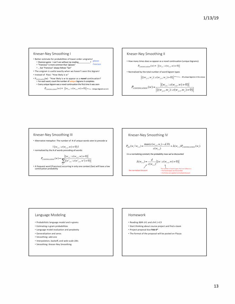
• Better estimate for probabilities of lower-order unigrams!• Shannon game: I can’t see without my reading___________?• “Francisco” is more common than “glasses”• … but “Francisco” always follows “San”

• The unigram is useful exactly when we haven’t seen this bigram!• Instead of P(w): “How likely is w”

• Pcontinuation(w): “How likely is w to appear as a novel continuation?• For each word, count the number of unique bigrams it completes• Every unique bigram was a novel continuation the first time it was seen

Francisco

Kneser-Ney Smoothing I

glasses

PCONTINUATION (w)∝ {wi−1 : c(wi−1,w)> 0} Unique bigrams w is in

Kneser-Ney Smoothing II

• How many times does w appear as a novel continuation (unique bigrams):

• Normalized by the total number of word bigram types

PCONTINUATION (w) ={wi−1 : c(wi−1,w)> 0}

{(wj−1,wj ) : c(wj−1,wj )> 0}

PCONTINUATION (w)∝ {wi−1 : c(wi−1,w)> 0}

{(wj−1,wj ) : c(wj−1,wj )> 0} All unique bigrams in the corpus

Kneser-Ney Smoothing III• Alternative metaphor: The number of # of unique words seen to precede w

• normalized by the # of words preceding all words:

• A frequent word (Francisco) occurring in only one context (San) will have a low continuation probability

PCONTINUATION (w) ={wi−1 : c(wi−1,w)> 0}{w 'i−1 : c(w 'i−1,w ')> 0}

w '∑

| {wi−1 : c(wi−1,w)> 0} |

Kneser-Ney Smoothing IV

PKN (wi |wi−1) =max(c(wi−1,wi )− d, 0)

c(wi−1)+λ(wi−1)PCONTINUATION (wi )

λ(wi−1) =d

c(wi−1){w : c(wi−1,w)> 0}

λ is a normalizing constant; the probability mass we’ve discounted

the normalized discountThe number of word types that can follow wi-1

= # of word types we discounted= # of times we applied normalized discount

Language Modeling


Homework

• Reading J&M ch1 and ch4.1-4.9• Start thinking about course project and find a team• Project proposal due Feb 6st

• The format of the proposal will be posted on Piazza

lm · 2019-04-05 · 1/13/19 6 google n-gram release •serve as the incoming 92 •serve as the...

Documents