ljoel harbour, cdr, usn
TRANSCRIPT
Analyzing the Effects of Component Reliability onNaval Integrated Power System Quality of Service
by
Benjamin F. HawbakerB.S., Naval Architecture
U.S. Naval Academy, 2003
Submitted to the Department of Mechanical Engineering and the System Design andManagement Fellows Program in Partial Fulfillment of the Requirements for the Degrees of
Naval Engineerand
Master of Science in Engineering and Managementat the
MASSACHUSETTS INSTITUTE OF TECHNOLOGYJune 2008
02008 B.F. Hawbaker. All rights reserved.The author hereby grants to MIT and the US Government permission to reproduce and todistribute publicly paper and electronic copies of this thesis document in whole or i pa.
Signature of Author ........................ ....... ...Department of Mechanical Engineering and
System Design and ManagementJ-May 9, A08
Certified by ......................................... -. -....lJoel Harbour, CDR, USN
Associate Professor of the Practice of Naval Construction and EngineeringThesis Supervis,
Accepted by........................................ .............. .. ~k a --
Director, System Design and Management Fellows ProgramAngineering Systems Division
Accepted by ............................... .. ......Lallit Anand
Chairman, Committee on Graduate Students-•pnartmpnt nf Mpthaninr l EPn ineerin
OF TEOHNOLOGY
JUL 2 9 2008
LIBRARIES--

AbstractThe Integrated Power System (IPS) is a key enabling technology for future naval vessels
and their advanced weapon systems. While conventional warship designs utilize separate powersystems for propulsion and shipboard electrical service, the IPS combines these functions. Thisallows greater optimization of engineering plant design and operations and leads to significantpotential lifecycle cost savings through reduced fuel consumption and maintenance.Traditionally the focus of power system design has been survivability, with the assumption thatservice continuity was inherently provided. A new probabilistic metric, Quality of Service(QOS), now allows the power continuity and quality delivered to loads to be addressed explicitlyduring the design of IPS vessels. This metric is based both on the reliability of the power systemcomponents and the system architecture employed.
This thesis describes and implements a method for modeling and evaluating the effects ofcomponent reliability on the QOS performance delivered by a current generation IPSarchitecture. First a representative "ship" is created, based largely on the U.S. Navy'sZUMWALT class destroyer (DDG-1000), including electrical loads, an operating profile, andIntegrated Fight Through Power system architecture. This simulated ship is then run through areliability analysis model employing Monte Carlo Simulation techniques to evaluate the QOSperformance of the power system. By treating the reliability of power system components as avariable, the model gives insight into the role component reliability plays within the givensystem architecture. A method is then proposed for extending this analysis to comparativestudies between future IPS architectures or components, with the ultimate goal of allowingresearch and development efforts to better focus precious funding and resources on areas withthe greatest potential for high-value improvement.

AcknowledgementsThe author would like to acknowledge the following individuals for their contributions and
assistance. Without them his thesis would not have been possible.
* CDR Joe Harbour, USN, Thesis Supervisor
* Pat Hale, Thesis Supervisor
* Dr. Tim McCoy, Thesis support and inspiration
* CAPT Norbert Doerry, USN
* David Clayton
* Dr. John Amy
* CAPT Pat Keenan, USN
* Anna and Sophia Hawbaker, for their unwavering support

Biographical NoteLT Benjamin Hawbaker, USN, graduated from the U.S. Naval Academy with a B.S. in Naval
Architecture in 2003. He is currently a member of the U.S. Navy Engineering Duty Officer
community enrolled in the MIT Naval Construction and Engineering Program and is also a
System Design and Management Fellow. Prior to becoming an Engineering Duty Officer, he
served as Anti-Submarine Warfare Officer on USS Oscar Austin (DDG-79). LT Hawbaker is a
member of the Society of Naval Architects and Marine Engineers and the U.S. Naval Institute.

Table of ContentsAbstract ........................................................................................................................................... 2
A cknow ledgem ents................................................................................................... ........... 3
Biographical N ote .................................................................................................... ........... 4
Table of Contents ....................................................................................................... ......... 5
List of Figures ........................................................................................................... .......... 7
List of Tables ................................................... 8
Chapter 1 - Introduction.......................................................................................................... 9
M otivation............................................................................................................. ........... 9
Background and Prior W ork ............................................. .................................................. 10
Objectives .................................................. 11
Thesis Outline .. ........................................................................................................ 12
Chapter 2 - Concepts & Theory .................................................................. ............................ 14
Integrated Pow er System s......................................................................................................... 14
Architecture of Integrated Pow er System s ..................................... .................. 16
Pow er Conversion M odules ................................................................. ........................... 19
Zonal Electrical Distribution and Integrated Fight Through Power .................................. 20
Quality of Service ..................................................................................................................... 24
Q O S Load Categories ................................................. .................................................... 25
Load Shedding ...................................................................................................................... 26
Basic Q O S Calculation ................................................ ................................................... 27
Reliability.................................................................................................................................. 29
Failure and Failure Rates .................................................................. .............................. 29
Probability D istributions .............................................. ................................................... 31
A vailability ........................................................................................................................... 33
Chapter 3 - M odeling & Sim ulation........................................ ............................................... 34
Approach.......................................... 34
M odel Ship D esign ................................................................................................................... 35
IPS System D esign.................................................................................................................... 41
Com puter Sim ulation M odel .................................................................. ............................ 43
D esign of Experim ents.............................................................................................................. 53
Chapter 4 - Results & A nalysis .................................................................. ............................ 55
Experim ental Results & A nalysis ........................................................................ ...... . 55

Chapter 5 - Evaluation & Conclusions................................................................................... 61
M odel Evaluation...................................................................................................................... 61
Applications of the Model .................................................................................................. 63
In Conclusion........................................ 65
R eferences ....................................................................... ............................ ............................ 66
Appendix I- Ship Service Electrical Loads ........................................................................ 69
Appendix II - Simulation Model Code......................................................................................... 71
Mission Array Creation Module: missionmod ......................................... ........... 71
Power Load Array Creation Module: loadmod ......................................... .......... 72
Power Generation Capacity Array Creation Module: pgmmod .................................... . 74
Power System Availability Array Creation Module: relymod ..................................... . 75
Power System Operational Evaluation Module: pwrsysmod ..................................... . 76
Quality of Service Failure Evaluation Module: qosmod ..................................... ... 78
Master Simulation Module: MonteXX ..................................... ...... ............... 79
Appendix III - Simulation Output Data........................................................................................ 81
List of FiguresFigure 1 - US Navy Destroyers Installed Electric Generating Capacity (Amy, 2002, p. 331)..... 15
Figure 2 - AC Radial Distribution (Hegner & Desai, 2002, p. 336).................................. 21
Figure 3 - AC ZED (Hegner & Desai, 2002, p. 337).................................. ............. 21
Figure 4 - Current Generation IFTP System (Doerry, 2007, p. 25)................................... 22
Figure 5 - Proposed Next Generation IFTP Zonal Architecture (Doerry, 2007, p. 27)................ 23
Figure 6 - The Bathtub Curve (Wilkins, 2002)............................... ..... ................. 30
Figure 7 - Typical Bathtub Curve for Electronic Components.......................... ......... 31
Figure 8 - Exponential Distribution: PDF, Reliability, and Failure Rate vs. Time .................. 32
Figure 9 - Converteam Advanced Induction Motor (Converteam, 2006) ................................ 36
Figure 10 - Shipwide IPS Architectures ...................................................... 41
Figure 11 - Zonal IPS Architecture....................................... ................................................. 42
Figure 12 - Simulation Model Architecture...................................................................... 46
Figure 13 - JMP Profiler Output for PGM and Power Conversion Component Types as Variables
....................................................................................................................................................... 5 7
Figure 14 - JMP Profiler Output for PDM Component Types as Variables........................... 58
List of TablesTable 1 - Operating Conditions..................................................................................................... 39
Table 2 - Speed-Derived PM M Loads .......................................................... ........................ 40
Table 3 - PMM Loads by Operating Condition .................................... .... .............. 40
Table 4 - Zonal SSCM / SSIM Requirements .................................... .............. 43
Table 5 - Load N odes.................................................................................................................... 48
Table 6 - Experiment Design Array (MTBF in 103 hours)................................ ......... 54
Table 7 - Collected Experimental Response Data ........................................ ............ 56

1
Chapter 1 - Introduction
Motivation
For much of the history of the modem warship, the archetypal design has consisted of a
set of engines dedicated exclusively to propulsion and an additional set of engines dedicated to
function as generators to supply electrical power to the vessel. This approach made sense
initially, when electric loads required only a tiny fraction of the power necessary to propel the
ship. The increasing role of electronics, computers, and power-intensive weapon systems has led
to a steadily growing demand for electrical power on warships, to the extent that a new model
has emerged and is rapidly gaining acceptance. The integrated power system (IPS) takes the two
ultimate destinations for power generated on a vessel and allows power from all the vessel's
engines to be used for either purpose. The basic principles of this concept are now well
understood, but constant advances in the technology utilized by IPS systems (as well as
traditional shipboard electrical systems) present new challenges for designers. Additional
complications arise from the increasingly finicky nature of the sophisticated computer systems
that make up more and more of the electric loads. These systems require high quality power, and
have little or no ability to tolerate interruptions in this power. Survivability has been the driving
factor in nearly all previous electrical system designs, but can no longer be the sole focus for
designers of future warships. While survivability obviously remains crucial for any future
system, increasing importance must be placed on what can be called electrical system quality of
service (QOS). The motivation for this study is to examine several of the factors which
influence this quality of service in IPS ship designs and assess their roles and relative importance

in order to aid designers in focusing future design efforts and research initiatives on the areas in
which they can be most effective.
Background and Prior Work
Traditionally, the primary focus of naval electrical system design has been on
survivability during battle or other damage scenarios. The continuity and quality of the power
delivered during normal operations was seldom considered explicitly. Instead designers relied
on basic rules of thumb and simplistic redundancy rules to ensure the day-to-day power system
operating characteristics would be acceptable. For a long time, this approach was perfectly
acceptable, as electrical systems were only a small portion of the overall ship, were limited in
scope to command and control or combat systems roles, and were generally designed from the
ground up for their specific platform and function. Over the past few decades, however, the role
and nature of shipboard electronics have undergone drastic changes. Warships have come to rely
increasingly on computers and other electronics in nearly all ship systems. Additionally, to
reduce development and procurement costs, more and more systems are being adapted for naval
use from non-military designs - commonly referred to as commercial-off-the-shelf (COTS)
systems. These new systems are considerably less rugged and much more demanding in terms of
the quantity and quality of power they require. At the same time their near ubiquity means that
for a new ship to function effectively, its power system must be designed to meet the increased
demands of its electrical loads, not vice versa. The situation is further complicated when
considered within the framework of an integrated power system. The propulsion motors demand
large quantities of electrical power in an inconsistent and highly unpredictable manner, and can
also create significant harmonic distortions and other impacts to power quality if not properly
addressed in the system design. Clearly the traditional way of doing business is no longer
adequate.
While the ultimate purpose is not new, the idea of service quality as a design variable was
not broached until 2005, when CAPT Norbert Doerry and Mr David Clayton, both of the Naval
Sea Systems Command addressed "the practical design issues associated with providing
continuity of service under other than combat damage conditions and [proposed] a Quality of

Service (QOS) metric to aid in the design, design certification and operation of shipboard power
systems" and further defined the metric as "based on the probability that the power system will
provide the continuity of power that each load needs to support the ship's missions" (2005, p. 1).
This paper, presented at the IEEE Electric Ship Technologies Symposium, represented a first
step in addressing the issues created by the evolution of naval power systems. Since its
publication, although the authors have continued to refine the concept of QOS in several papers,
little attention has been paid to the subject in other published work. The need for additional
work to examine the role of QOS, and the factors that influence it, is clear. Doerry lists several
of these factors, stating "the reliability of power system equipment, the systems architecture of
the power system, and the power system concept of operation are the primary drivers for QOS
provided by the power system" (2007, p. 29). The first two of these factors will be the focus of
this study, in an effort to explore the nature of QOS and recommend ways to use and improve
this new metric in future ship design efforts.
Objectives
Since it is a new concept that has not been included in previous design efforts, there are no
tools available to the author to model QOS effects specifically. Therefore, the first goal of this
project is to develop a basic modeling approach to simulate power system operation and QOS
effects in an IPS ship. The model must replicate the major components of the power system, as
they pertain to QOS, including the power system architecture, component characteristics,
propulsion and ship's service loads, and operating profile. While it is important to generate a
fairly representative model of the ship, it is not necessary to model any particular ship or to
reproduce any system exactly. This is in fact impossible in an academic setting due to the
classified and/or proprietary nature of much of the information required for such detail. The key
is instead to develop a model that includes representative system elements and is scalable,
providing a building block for future work, where access to exact system and component
specifications may not be an issue. The model also does not need to extend beyond the realm of
QOS. It should be used to simulate QOS performance, but other unrelated power system
evaluations would be left for different programs. This model is envisioned as simply a QOS
module within a broader power system design and evaluation tool.
Once a functional model has been developed, the next objective will be to study the role of
component reliability throughout the power system. As hard reliability data is difficult to obtain,
and what is available is often suspect due to the varying methods and assumptions used in its
estimation, reliability will be treated as a variable. One goal of this portion of the study will be
to locate critical component levels where reliability is very important. In other words, to
determine the system elements whose individual reliability level impacts QOS the most. In the
same way, the study will attempt to locate component levels whose reliability has a markedly
small impact on system QOS. The purpose of both these efforts will be to find areas of high-
value reliability, where small local improvements can lead to greater global system benefits, or
conversely where small global QOS sacrifices could yield great costs savings through reduced
component reliability. These areas would then be recommended as focal points for future
reliability research in order to improve QOS and cost performance.
The third objective will be to propose methods and applications for evaluating the influence
of changes in component characteristics or the IPS system architecture on QOS performance
using the developed model. This will include the effects of changes in redundancy, such as
shifting from an N+I approach to another method. It will also involve investigating the impacts
of proposed technologies, particularly new power conversion elements, on the IPS architecture
and QOS. Possibly the most significant impact would be the switch from medium voltage AC to
medium voltage DC or high-frequency AC as the primary source power. Again the goal is to
develop a method for finding high-value aspects of IPS system architecture that can be
recommended for future efforts to improve QOS and cost performance.
Thesis Outline1. Review relevant theory and concepts
a. IPS Concepts
b. QOS Concepts
c. Reliability
2. Modeling and Simulation
a. Ship Model Design

b. IPS System Design
c. Computer Simulation Model
d. DOE simulation plan
3. Simulation Results and Analysis
4. Evaluation and Conclusions
a. Model Evaluation
b. Applications for the Model
c. Conclusion

2
Chapter 2 - Concepts & Theory
Integrated Power Systems
From the first introduction of electric systems onboard a naval warship, the USS Trenton
and its electric lighting installed in 1883, the dominant design paradigm has consisted of large
main engines providing propulsion power and separate, usually much smaller engines generating
electrical power for the use of other ship systems. Even on ships with a common power source
such as steam, separate turbines or other systems are used to power propulsors and electric loads,
resulting in limits on each. For a long period of time, this dichotomy presented few problems.
The relative amount of power necessary to propel a ship through the water has not changed that
significantly since the late 19th Century. The same cannot be said, however, of electrical power.
Shipboard electrical systems evolved gradually at first from lighting to radio communications, to
radar and sonar and other early electric systems. As the computer age dawned this growth began
to accelerate rapidly. Figure 1 illustrates the rapid increase in generation capacity, which
corresponds with electric loads, over the past few decades. On a modem warship, the electric
loads can be expected to make up easily ten percent or more of the total power produced by a
ship's engines (propulsion and ship's service combined).
As the demand for electrical power continues to grow, the separation of the propulsion
and ship's service power functions creates increasing inefficiency. Both electrical service and
propulsion loads tend to be highly variable in warships, depending greatly on the type of
operations being conducted, specific systems involved, and the maneuvers required. Both types

of power system must be sized for worst case scenarios, resulting in a ship that has far more
power generation capacity than it needs at nearly any time. This leads initially to higher
acquisition cost for more or larger engines, and ultimately to higher operating costs due to more
engine hours and frequent operation at suboptimal loading points. There is no reason to believe
electrical load demands will stop growing at anytime in the foreseeable future. Thus continued
adherence to the traditional design paradigm will lead these inefficiencies to climb well beyond
acceptable levels.
wJJ
Ipam
, wo
IiZ
#oti
ao
I0
Year of aItroductlon
Figure 1 - US Navy Destroyers Installed Electric Generating Capacity (Amy, 2002, p. 331)
As the impending problems with current power system design became apparent, a
solution to the inefficiencies of dual systems emerged in the form of the integrated power system
(IPS), which began to garner widespread support starting in the 1990s. While the idea of electric
propulsion is not new, recent advances in power electronics were necessary to make it a feasible
option for large, high speed vessels. Although it goes by several different names, including
Integrated Electric Propulsion (IEP), Integrated Full Electric Propulsion (IFEP) and Integrated
Electric Drive (IED), the basic IPS concept is the same. Several prime movers (engines),
potentially of different types and sizes, are used to generate electrical power, which is then sent
via a common distribution system to both the propulsors (now electric, not mechanically driven)
and the ship's service loads. This arrangement allows tremendous operational flexibility and

great potential gains in operating efficiency over traditional separated systems. The concept has
already gained commercial acceptance in several areas, including cruise ships, ferries, and many
other vessel types. Now several navies, including the US, UK, France, and the Netherlands, all
have programs exploring (and building) IPS warships.
There are several key benefits to the IPS architecture. The first advantage comes from
the improvements in operational efficiency and lifecycle cost. By operating the lowest number
of prime movers necessary, engine hours are cut for all engines, thus reducing wear and
maintenance. The engines in operation can also be run at higher loading levels, maximizing their
fuel efficiency. Additionally, due to the more efficient operation, with proper planning the total
number of installed prime movers can be reduced. This can result in considerable savings of
volume and complexity, as well as to both acquisition and lifecycle costs. Another advantage is
the ease of reversing the direction of shaft rotation using power electronics. This eliminates the
need for the complex, fragile, less efficient controllable-pitch propeller (CPP) common in
modem warship designs. Although electric transmission is less efficient than mechanical
transmission at full power (89% vs. 93% for a CPP ship), this is mitigated by improved low
speed efficiency that can match or even exceed CPP transmission (Hodge & Mattick, The
Electric Warship, 1996). A final advantage comes in the form of design flexibility. With
electric transmission, there is no need for long, heavy shafts between engine and propeller.
Besides allowing engine placement for operational and survivability considerations, this also
saves considerable weight and volume, while reducing design and construction costs. The
primary disadvantages of an IPS warship involve the size and cost of currently existing
propulsion motors and power conversion equipment. Presently these downsides effectively
cancel out a fair portion of the gains from IPS. However efforts are underway to overcome these
obstacles, and the ever-advancing state of power electronics technology bodes well for success in
the near future.
Architecture of Integrated Power SystemsThe current US Navy IPS architecture consists of several functional modules that perform
the various roles within the power system. These modules were defined by CAPT Norbert
Doerry, USN of the US Naval Sea Systems Command in establishing a program known as the
Next Generation Integrated Power System (NGIPS). In two reports, "Establishing The Next

Generation Integrated Power System Baseline Architecture" (2007) and "Next Generation
Integrated Power System Technology Roadmap" (2007), Doerry laid out and then refined the
functional modules that make up a notional IPS system.
The first module is the power generation module (PGM). The function of the PGM is
fairly self-explanatory; it converts fuel into electrical power. The PGM would typically consist
of a prime mover and a generator set, as well as the necessary power rectification, auxiliary
support, and control equipment. While gas turbine or diesel engines are the most common
concept for the prime mover, hydrogen fuel cells and nuclear power represent other realistic
options for future PGM use.
The next module is the propulsion motor module (PMM). Its function, naturally, is to
convert electrical power into rotational motion to drive the vessel's propulsor. It generally
consists of a motor drive and an electric motor. The current state of the art is known as the
Advanced Induction Motor (AIM), but future IPS systems may use more advanced motors using
permanent magnets or high-temperature superconductors. The goal of these new technologies is
to increase power density, a necessity for employing IPS in smaller, high-speed warships.
While the PMMs are the destination for much of the generated power, the power load
module (PLM) represents the remaining loads, and will continue to grow in size relative to the
PMM portion of the overall demand. More of a function placeholder than a specific system, the
loads that make up the PLM are designed for their role within the ship's mission, with little
regard for their place within the overall power system. The key task within the PLM therefore is
not design but organization. The ship loads must be classified in terms of several different
schemes, including power type, mission priority, and QOS. The various categories each PLM
load falls into are then used for sizing generation and distribution equipment as well as load
shedding in the event of failure or damage. Classifying loads within the PLM will be
complicated even further as new sensor and weapon technologies are developed and fielded.
The immense power requirements and unique load profiles of the advanced radar systems, rail
guns, and directed-energy weapons envisioned for future warships will cause them to interact
with the IPS system in ways unlike any current PLM loads. It is likely that a new Special Loads
Module will be necessary to account for these exceptional loads within the IPS framework.

Power is transferred between various modules by elements of the Power Distribution
Module (PDM). The PDM function is carried out by the cables, switchgear, and fault protection
equipment necessary for each type of power encountered through the system. Because the PDM
encompasses all power at all transfer points, there is considerable variation in the requirements it
must meet. It consists of everything from simple cables to complex load centers.
For power to be distributed and used effectively, it must assume different forms. The
power conversion module (PCM) is where power is converted from one such form into another.
PCMs are connected to other modules and each other by PDMs. Generally PCMs consist of
either transformers or solid state conversion elements. Where conversion is necessary as part of
another module's basic function, such as power generation or motors, it is included within that
module, and not considered to be a separate PCM.
A crucial aspect of any integrated power system is system control. The module
responsible for coordinating the actions and responses by and between other functional modules
is the power control module (PCON). Unlike the other modules, the PCON is not necessarily a
physical entity, but instead is comprised of the software needed to control and monitor the
remainder of the system. Portions of the PCON module may lie within the physical domain of
other modules, or they may reside in a separate hardware system (such as a central control
console). Some portions of the PCON may be automatic, while others will involve a human
interface. The functions defined for PCON within the NGIPS framework include: remote
monitoring and control of other modules, mobility control, resource planning, system
configuration, fault detection and isolation, load shedding (based on mission priority or QOS),
supporting maintenance and tag-out efforts, and training.
The final functional module is the energy storage module (ESM), which is responsible for
storing excess power to be used later or to accumulate large quantities for special purpose loads.
Although not part of any currently planned IPS system, ESMs are expected to play a crucial role
in fielding many new technologies aboard IPS vessels, including fuel cell PGMs and high power
directed energy or electromagnetic weapon systems. There are numerous forms that an ESM
could take, including a simple battery bank, a flywheel, or a large capacitor. Future IPS systems
may employ ESMs only for special loads or use them as system-wide sources of standby power.

Power Conversion ModulesWithin the context of this paper, the only functional module necessary to discuss in detail
is the power conversion module. There are currently three main types of PCM used within the
IFTP framework, delineated by number, PCM-1, PCM-2, and PCM-4; and their proposed
follow-on PCMs, PCM-1A and PCM-2A, and PCM-4A. An excellent description of each PCM
is found in the "NGIPS Technology Development Roadmap":
PCM-4: Transformer Rectifier to convert MVAC power to 1000 VDC power. The ratingof the PCM-4 must be greater than '/2 of the maximum margined electrical load andgreater than the total un-interruptible load. Under normal operation, two PCM-4s will beoperational, each supplying power to one of the port / starboard longitudinal busses.
PCM-1: Converts 1000 VDC Power from PCM-4 to 800 VDC power, 650 VDC Power,or another user-needed DC voltage. Also segregates and protects the Port and Starboard1000 VDC Busses from in-zone faults. 650 VDC Power used to supply power to motorcontrollers for large motors and for large resistive heating applications PCM-1 contains anumber of modular Ship Service Converter Modules (SSCM) that can be paralleled toprovide redundancy and the requisite power rating. Each SSCM currently has a rating of300 kW and uses a proprietary interface with the PCM-1 cabinet. SSCMs can providepower to segregated outputs. For each segregated output, with one SSCM out of service,the remaining SSCMs shall be able to supply the greater of 50% of the maximummargined load or 100% of the maximum margined un-interruptible load serviced by thatsegregated output. (The 2nd PCM-1 in the zone will supply the other 50% of the load)
PCM-2: Converts 800 VDC power from PCM-1 into 450 VAC Power at 60 Hz. or 400Hz. Although a zone may have multiple PCM-2s, cost savings can be realized bylimiting the number of PCM-2s necessary to achieve survivability requirements. PCM-2contains a number of modular Ship Service Inverter Modules (SSIM) that can beparalleled to provide redundancy and the requisite power rating. Each SSIM currently hasa rating of 300 kW and uses a proprietary interface with the PCM-2 cabinet. SSIMs canprovide power to segregated outputs. For each segregated output, with one SSIM out ofservice, the remaining SSIMs shall be able to supply the maximum margined loadserviced by that segregated output.
PCM-4(A): Transformer Rectifier to convert MVAC/HFAC/MVDC power to 1000 VDCpower. The functionality of the PCM-4 may be incorporated into PCM-lA.
PCM-1A: A PCM-lA converts 1000 VDC Power from PCM-4 or power fromMVAC/HFAC/MVDC to 750-800 VDC power, 650 VDC Power, another user-neededDC voltage, or 450 volt 60 Hz AC Power. Also segregates and protects the Port andStarboard busses from in-zone faults. 650 VDC Power is used to supply power to motorcontrollers for large motors and for large resistive heating applications For DC loads,PCM-lA contains a number of modular Ship Service Converter Modules (SSCM) thatcan be paralleled to provide redundancy and the requisite power rating. Similarly, for AC

loads (short-term and long term interrupt 60 Hz loads) PCM-1A contains a number ofmodular Ship Service Inverter Modules (SSIM) that can be paralleled to provideredundancy and the requisite power rating.
PCM-2A: Converts 750-800 VDC power from PCM-1 into 450 VAC Power at 60 Hz,400 Hz, or variable frequencies and voltages to drive variable speed motors. PCM-2Awould be used to service un-interruptible AC loads as well as loads with special powerrequirements. One notable difference from the current PCM-2 is that the PCM-2A wouldincorporate the features of a load center - individual loads, or sets of small loads, wouldhave individual power converters. To enhance survivability, a zone could have multiplePCM-2As collocated with the serviced loads. In general, the number of loads serviced byPCM-2A should be minimized due to:
1. The efficiency of the current generation air-cooled input and output modulesfor the PCM-2A is considerably less (-85%) than the efficiency of the watercooled PCM-1A (- 97%)2. Since each of the output modules of the PCM-2A directly drives a load, N+Iredundancy is not provided. The reliability of the output modules of the PCM-2Awill directly impact the QOS provided to loads.3. The cost of providing power to loads from PCM-lA will be less than the costof providing power from PCM-2A via PCM-1A. (Doerry, 2007, pp. 24-26)
Zonal Electrical Distribution and Integrated Fight Through PowerA key enabling concept for the integrated power system is zonal electrical distribution
(ZED). Shipboard electrical distribution traditionally involved a radial system wherein AC
power generation units fed power through switchboards and then directly out to load centers
throughout the ship. This approach involved considerable complexity as well as large quantities
of cable and other distribution equipment to ensure sufficient survivability and service continuity
(Hegner & Desai, 2002). Figure 2 shows a typical radial AC power distribution system.
A considerable improvement over radial distribution was introduced aboard USS OSCAR
AUSTIN (DDG-79), launched in 1998, in the form of the AC ZED. This system supplies power
to several electrical zones via longitudinal busses. Load centers within each zone then distribute
the power to loads inside the zone. This architecture results in a much simpler system due to the
much shorter and more direct cable runs within the zones, saving weight and also construction
cost since cables can be run within zones before they are joined together. Figure 3 shows a
typical AC ZED system with four zones.

NAUMLIARYI Dnrfll I MAC~iH~M
AUEILIARYLMACHIAY
Figure 2 - AC Radial Distribution (Hegner & Desai, 2002, p. 336)
AN EECTRICALZONE
AN" ~CAL
Figure 3 - AC ZED (Hegner & Desai, 2002, p. 337)
From the AC ZED came the inspiration for the latest distribution scheme, a DC ZED
system known as Integrated Fight Through Power (IFTP). In IFTP power from the generation
modules is converted from medium voltage AC (MVAC) power, usually either 4.16kV or
13.8kV, into 1000 VDC power by PCM-4s, one for each of the two longitudinal DC busses.
Within each zone, the tie in to each bus is a PCM-1, which converts the power to lower voltage
DC using modular SSCMs and also isolates the bus from in-zone disturbances. From the PCM-
1, power is either distributed to DC loads or transferred to the PCM-2. The PCM-2 converts 800
VDC power from the PCM-1 into 450 VAC at 60Hz or 400Hz using modular SSIMs. From the
PCM-2 power is distributed via a load center to the AC loads within the zone. Within each zone,
vflw" 11
AN RECTRICAL,"Mons

the PCM-2 and any DC loads requiring multiple power sources are connected to both PCM-1s
and receive power via auctioneering diodes. A three zone IFTP system is shown in Figure 4.
MVAC
Figure 4 - Current Generation IFTP System (Doerry, 2007, p. 25)
IFTP provides several advantages over AC ZED systems. The first results from cost
savings from removing the large electromechanical switchgear needed for AC distribution and
instead using power electronics to perform fault protection. The "fight through" capability
comes from the zonal isolation afforded by the PCM-ls connecting each zone to the longitudinal
DC busses. Additional savings are realized by eliminating the need to generate and distribute
high quality AC power to the entire ship. This means that the generator operating frequency is
less constrained, allowing the use of smaller, less expensive rectification equipment. By
converting to the necessary power type within zones, power quality delivered to the loads is also
higher than when converted at the source as in either AC distribution scheme. Another benefit is
in the simplicity and speed of the auctioneering diodes used to transfer power between port and
starboard buses (via PCM-1s), which are smaller, cheaper, and faster than the bus transfer

switches utilized in AC ZED. A final, and perhaps the most significant, benefit of IFTP is its
potential to take advantage of the rapid advances in power semiconductor technology to improve
both capacity and performance (Hegner & Desai, 2002, pp. 337-338).
While the present IFTP system possesses a number of significant advantages over
previous AC distribution schemes, the proposed next generation IFTP architecture, utilizing
PCM-1A, PCM-2A, and possibly PCM-4A, will offer even greater benefits. If PCM-4A is not
used but instead incorporated within PCM-1A, only the high power bus (as opposed to both high
power and 1000 VDC busses in the current IFTP) will need to cross zonal boundaries, reducing
cabling and improving survivability. It will also result in lower total required transformer
rectification capacity between the PCM-1As than the PCM-4 (since each PCM-4/4A must be
sized for 50% of the maximum margined ship's service load). In addition to potentially
eliminating many types of special purpose load conversion equipment, savings are realized by
reducing the total number of SSCMs required in the PCM-1A, since SSCMs are no longer
required to power all SSIMs downstream in the PCM-2A (Doerry, 2007, p. 27). Figure 5 shows
the nominal in-zone architecture of this system.
MVACHFACHVDC
or1000 VIDvia PCM
MVACHFACHVDC
or000 VDCia PCM-4
Laud
Figure 5 - Proposed Next Generation IFTP Zonal Architecture (Doerry, 2007, p. 27)

Quality of ServiceDoerry and Clayton (2005) define Quality of Service as a metric to evaluate the
continuity of service provided by the power system. It is based on the probability that each load
will be provided with the level of continuity it needs to effectively fill its role within the ship's
mission. The major factors involved with QOS include the capacity rating, reliability, and
failure mode of the PGMs, PCMs, and PDMs, and their respective submodules, as well as the
overall system architecture and the current operational configuration of the power system.
This definition of quality is in contrast to the concept of power quality from a terrestrial
power grid perspective. In this sense, power quality refers to variations in the characteristics of
the actual voltage delivered from the ideal prescribed voltage (generally a perfect sine wave at
60Hz). These variations can include electrical noise, momentary interruptions, momentary sags
or surges, transients ("spikes"), and harmonic distortion (Salem & Simmons, 2000). These
characteristics of the voltage delivered are of great importance for terrestrial power supplies
which must generate and transmit large quantities of power over long distances to many users.
They are still important considerations in shipboard systems, but are less critical for engineers,
particularly in an IFTP system where the needed power is created (or, more properly, converted)
in close proximity to the load and in relative isolation.
At its simplest, Quality of Service can be viewed as a failure rate of the power system
from the perspective of its loads. A failure would consist of any power interruption or departure
from the required power quality (in the terrestrial sense) that causes the load to be unable to
perform its required function. The causes of such failures might include equipment failure in any
of the IPS modules or submodules or transient conditions resulting from normal system
operations. While these conditions might occur to some degree with relative frequency, they will
not necessarily result in a QOS failure as defined above. If the system is able to maintain the
required level of service through another path or temporarily shedding loads, no failure will have
occurred. Likewise if the load's mission does not require urgent restoration of power, manual
corrective actions or even repairs could bring the system back online before a QOS failure
occurs. This might be the case for temperature control loads, such as heaters, air conditioners, or
refrigeration, where significant time periods can elapse before the temperature in their
compartments changes appreciably (Doerry & Clayton, 2005).

QOS Load CategoriesTo account for these variations in tolerance, Doerry and Clayton (2005) proposed a set of
load categories based primarily on the time before a QOS failure can be considered to have
occurred.
A. Uninterruptible Load
Uninterruptible (UI) Loads are electrical loads which cannot tolerate a power
interruption lasting 2 seconds. These loads generally require a source of standby power,
whether through an uninterruptible power supply (UPS) or some sort of alternate path
control by fast automatic switches like auctioneering diodes. These loads should be
capable of withstanding interruptions on the order of 10 ms while switching to the
standby power supply.
B. Short-Term Interrupt Load
Short-Term Interrupt (STI) Loads are loads capable of tolerating a 2 second
service interruption, but incapable of tolerating interruptions longer than 5 minutes in
duration. These loads are generally provided with standby power through slower
electromechanical switchgear, which imposes the minimum 2 second requirement. This
allows switching, fault clearing, and load shedding of Long-Term Interrupt Loads before
power is guaranteed to the STI Loads. The 5 minute limit is considered to be the nominal
startup time for a standby generator to be brought online.
C. Long-Term Interrupt Load
Long-Term Interrupt (LTI) Loads are loads which are capable of tolerating
interruptions longer than 5 minutes. They may be provided with a source of standby
power, but not necessarily. LTI loads are the first loads to be shed in order to maintain
service to STI and UI loads. While bringing a standby generator online will often result
in power being restored to all loads in less than 5 minutes, the LTI loads may be subject
to additional load shedding if necessary due to continued limits on the power, for instance
if the standby generator is smaller than needed.

D. Exempt Load
Exempt Loads are not quite the same as the three previous load categories.
Exempt loads can be considered a second class of LTI load, and only exist for the
purpose of generator sizing. While ship's service loads must fall into one of the three
standard QOS load categories, propulsion loads may not. A certain quantity of
propulsion power might be designated as STI, perhaps to maintain steerage or some
minimum speed. The rest would be considered LTI or exempt. The portion of this
remaining propulsion load that cannot be delivered with the largest generation module
out of service would be categorized as the exempt load.
Load SheddingIn the event of a failure within the power system, the available power may be less than
the power required by the online loads. In order to provide power to the most important online
loads, it may be necessary to deny power to certain loads in a process called load shedding.
Doerry and Clayton (2005) define two types of load shedding that may be conducted by an
integrated power system.
A. Quality of Service Load Shedding
QOS load shedding is based on the QOS load categories defined above. When a
power interruption first occurs within the system, affected UI loads receive power from
their UPS or fast-switching standby immediately. The system then conducts load
shedding of LTI loads in order to provide sufficient power to the STI loads online.
During this period repairs can be made or additional generation capacity can be brought
online, with the goal of restoring sufficient power to all loads within the 5 minute Long-
Term Interrupt limit. If this process occurs without further mishap, there is a high
likelihood that a QOS failure will be avoided.
B. Mission Priority Load Shedding
In the event that sufficient power capacity cannot be delivered to all required
loads within the 5 minute LTI time limit, the power system shifts its load shedding focus
from QOS to Mission Priority load shedding. Mission priority load shedding ensures that

the most important load systems, as dictated by the ship's current mission, are given
power first, regardless of QOS category. This means that power may be restored to
certain LTI loads, while UI or STI loads are shed. The need for Mission Priority load
shedding may also arise within the LTI time limit if the available power is insufficient for
the online STI and UI loads. In this situation STI loads would first be shed according to
Mission Priority, followed by UI loads. By definition, all situations requiring a shift to
Mission Priority load shedding also involve a QOS failure (including situations where
operators may force a shift to Mission Priority load shedding for tactical reasons).
Basic QOS CalculationGiven the complex nature of any integrated power system, calculating a value of QOS,
which can be equated to a mean time between unacceptable service interruptions, from any
perspective is certainly a nontrivial exercise. In "Designing Electrical Power Systems for
Survivability and Quality of Service," Doerry (2007) suggests a basic method for calculating
what he refers to as a Mission System Quality of Service. This model relies on simple
summations and several simplifying assumptions, including a known, fixed mean time between
failures (MTBF), a small mean time to repair (MTTR) relative to MTBF, and treats component
failure as the only source of QOS failure. The goal of this project is to improve upon this basic
method, applying stochastic simulation methods and avoiding these simplifying assumptions if
possible. The method for accomplishing this will be discussed in detail later in the paper. The
basic Mission System QOS model proposed by Doerry is shown below.
a. Ship Concept of Operations in the form of percent underway time the ship will be indifferent operational modes. The fraction of time in an operational mode i is given byfom(i)
b. Mission System Quality of Service model for each operational mode. This model willprovide a "1" if a QOS failure has occurred for a given set of power interruptions ofspecified durations to one or more mission system loads (otherwise provides a "0"). TheMission System Quality of Service model is represented by qom(i,pi[k]) where i is theoperational mode, andpi[k] is a vector of power interruptions for the k mission loads.
c. Power System Concept of Operations that determines which power system componentsare online and in what configuration for each ship operational mode. pom(ij) returns thefraction of time that power componentj in operational mode i is online.

d. Power system Reliability Model that provides the MTBF rj for each power componentj where time is measured in hours that the component is on (operational time).e. Power System Fault Effects Analysis that determines for each failure of a powersystem elementj, the vector of power interruptions for each of the k mission loads: pij[k].
The fraction of time that a QOS failure will occur in response to the failure of powersystem componentj is given by
f qoi) X fo,,),Pom,, )qom(,.,, iRD
The fraction of time that componentj is on is given by
f, =I fonP)oM, J)i=
The MTBF of component j based on calendar time instead of operational time is given by
rc() -
Since the reciprocal of MTBF is the failure rate, then the QOS failure rate due to eachpower system component is given by
1 fqscj)
QOSJ r,( )
Thus the QOS provided to the mission system due to the failures of all power systemcomponents (measured as a [mean time between service interruptions]) is given by
1 f mf
os-=OS j.= rc(,)
(QOS
2
j-' rcU) (pp. 29-30)

Reliability
Failure and Failure RatesCentral to the quality of service delivered by an integrated power system is its reliability, which
is determined by both the architecture of the system and the reliability of the individual
components that make up the system. This section will concern itself primarily with the theory
necessary to investigate component reliability. A fairly standard definition for reliability in
engineering is provided by O'Connor (1991) who defines it as, "the probability that an item will
perform a required function without failure under stated conditions for a stated period of time"
(p. 3). Given this definition, it becomes necessary to further explore the nature of failure and its
expected behavior over time.
When discussing failure, it is often important to distinguish between repairable and non-
repairable items. For non-repairable items, the item will only fail once within its lifetime. For
such items, the instantaneous probability of this failure occurring is known as the hazard rate.
For repairable items, upon failure the item can be restored to functioning condition, and thus may
suffer multiple failures through its lifetime. Repairable items are subject to an instantaneous
failure probability known as the failure rate, sometimes also termed the rate of occurrence of
failures (ROCOF). The difficulty lies in determining what a repairable item is. This is often
based on the system level one wishes to examine. Drilling down far enough one will always find
a non-repairable item. In practice what we generally consider as the smallest elements of a
system are still in reality subsystems made up of even smaller elements. This is particularly true
for electronic systems. For the purposes of this study, all components will be treated as
repairable. While many elements may simply be replaced within the system following a failure,
there is a high likelihood they will be repaired and returned to the system when a similar
component fails. The existence of the US Navy 2M/ATE program for conducting electronics
repair onboard the ship (as opposed to at maintenance depots ashore) supports this assumption,
as does the increasing focus on employing hot-swappable components (e.g. the SSCMs within a
PCM-1A) which are replaced immediately and subsequently repaired outside the system to
minimize overall system downtime.

Regardless of their reparability, nearly all items exhibit a similar failure pattern over their
lifetime. This pattern is known as the bathtub curve, and is made up of three distinct parts, as
seen in Figure 6. The first portion of the bathtub is a period of decreasing failure rate known as
the infant mortality or wear-in period. During this time, early failure of defective members of
the item population is the dominant effect. This period is followed by a period (usually the
longest) of low, often near-constant failure rate known as the useful life. During this period
failures are primarily caused by external factors or extreme conditions and occur randomly with
roughly constant frequency. The final period is one of increasing failure rate known as the aging
or wear-out period. During this period failures due to cyclic loading and other time-dependent
stresses dominate.
The Bathtub CurveHypothetical Failure Rate versus TimetI
Wear-O utAilure Rate
Time
I.P0
M-i
Figure 6 - The Bathtub Curve (Wilkins, 2002)
While most items display the bathtub pattern, the actual shape of the various bathtubs can
differ dramatically. In the case of the electronic components being discussed here - and
particularly so for the components normally employed in naval power systems-, the typical
bathtub curve demonstrates very brief wear-in and wear-out periods separated by a long useful
life, as seen in Figure 7. The brief wear-in is mostly attributable to using mature designs and

good manufacturing practices, including bum-in, where defective components are revealed
before shipment to end users. The eventual wear-out is due primarily to heat effects on the
materials of surviving population members. The vast majority of failures for electronic items
surviving wear-in occur during the useful life period. These failures may be caused by extreme
loading or other external factors or they may be due to slight defects that manifest themselves
over time. Regardless of the exact source, they tend to occur randomly throughout the period
and at a constant rate (Lewis, 1996). This fact has important implications for the choice of
distribution used to model IPS component failure behavior.
Time
Figure 7 - Typical Bathtub Curve for Electronic Components
Probability DistributionsBy assuming that system elements are only present in the IPS system after they have
entered their useful life (i.e. inspection and bum-in have weeded out early wear-in failures) andalso assuming that Navy maintenance practices will result in replacement before age effectsdominate, we can thus reasonably assume a constant failure rate for all components consideredwithin the power system. This implies that the components exhibit memoryless behavior, or inother words the likelihood of failure during some future time period is independent of the itemsage. Furthermore, since the ship requires the use of its power system at all times, it can beconsidered to be continuously in operation.
The standard continuous probability distribution used to model constant failure ratebehavior is the single-parameter exponential distribution (hereafter simply the exponential

distribution). The exponential distribution is characterized by the constant parameter X, which isthe failure rate. The probability density function (PDF) for the time to failure is given by
f(t) = Ae-At
The cumulative density function (CDF), which represents the probability that failure hasoccurred by time t, is then calculated
F(t) = ft Ae-Atdl = 1 - e - At
The reliability, or the probability that the item has not failed by time t, is then calculated
R(t) = 1 - F(t) = e- At .
The expected value, commonly referred to as the mean time between failures (MTBF), or meantime to failure (MTTF) for non-repairable items, is calculated
MTBF = f R(t)dt = .
1 1The variance and standard deviation can then be calculated as T2 and - respectively. When
plotted versus time, the PDF and reliability for the exponential distribution take on the formsshown in Figure 8, while the failure rate plots as a horizontal line.
..... f(t)
......... R(t)
-" -- (t)
2/k 3/k
Figure 8 - Exponential Distribution: PDF, Reliability, and Failure Rate vs. Time
Another common distribution in reliability studies is the Weibull distribution. The
Weibull distribution, in either its two or three-parameter forms, is widely used due to its

versatility. By carefully choosing the parameters, the Weibull distribution can be used to model
the failure rates seen during wear-in or wear-out, and can also produce the constant failure rate
exponential distribution as a special case. It can also be used in situations where a threshold time
exists during which failure cannot occur. While the Weibull distribution is more versatile, the
exponential distribution is sufficient for this study, and so the more complicated Weibull will not
be discussed further.
AvailabilityA companion concept to reliability is availability, the probability that an item will be
available (i.e. able to operate) when required. Availability is normally applied only to repairable
systems, and in addition to the failure rate involves a repair (or replacement) rate for the item as
well. While generally a gross simplification, it is common to assume a constant repair rate, gt,
which is also modeled using the exponential distribution. The expected value of [t is known as
the mean time to repair (MTTR) and the two are inversely related, just as MTBF and X.
Instantaneous availability, the probability the item will be available at time t, can be calculated
using the expression
A(t) = + e-(A+11-)
which, as t becomes large, simplifies to the steady state availability
A(oo) = MTBFA+ MTBF+MTTR
Since availability is generally a very high number or percentage, it is often most instructive to
look at the unavailability, or downtime, of a system instead, which is simply 1-A. One common
problem when modeling availability is the fact that maintenance can take many forms and is not
as well studied or understood as failure. Attempting to model maintenance as other than a
simple MTTR, or including preventative maintenance or training can greatly increase the
complexity of the model. To avoid these complications, availability will only be examined in
this study in its simplest form.

3
Chapter 3 - Modeling & Simulation
Approach
In order to model the quality of service characteristics of an integrated power system, the
first step is naturally to select or create a power system to model. Due to the security issues
involved with using a current naval power system, it was clearly infeasible to model an existing
power system. The best and most expedient alternative was instead to develop a power system
based on current naval IPS design work and preliminary concept designs available in the public
domain. In addition to modeling the power system itself, a simulated "ship" with set equipment
and electrical and propulsion loads dictated by a mission profile was also necessary. Once the
required elements were created, a simulation model was developed, using a modular approach to
simplify coding, testing, and debugging. This simulation model was then used to run Monte
Carlo simulations of normal power system operations, using stochastic methods to examine
behavior patterns over a large number of similar, but randomly arranged events. The key input
variables to be examined through the model were component reliability levels. Even limiting the
model's focus to high-level components still resulted in too many components to evaluate all
combinations without excessive computing costs, and so Design of Experiments principles were
used to develop an experimental plan to evaluate the effects of component reliability. Once the
simulation runs were conducted for each individual trial of the experiment, the data could be
collected and analyzed to determine the importance of the reliability of each of the various
components on overall system QOS performance.

Model Ship Design
Worldwide the two primary IPS warship programs currently underway are the U.S.
Navy's DDG-1000 Zumwalt class, which is currently undergoing detail design, and the Royal
Navy's Type 45 Daring class, currently under construction and scheduled to commission in
2009. While the specifics of both ships' IPS systems are classified, sufficient publicly releasable
information is available that a representative power system could be designed based on either of
these vessels. The ready availability of DDG-1000 information and the author's status as a U.S.
Navy Engineering Duty Officer led naturally to its selection as the primary model for designing
the power system to be used within this study.
..One excellent source of data was a software program developed by the U.S. Naval Sea
Systems Command's (NAVSEA) Naval Surface Warfare Center, Carderock Division known as
the Advanced Surface Ship and Submarine Evaluation Tool (ASSET). ASSET is the Navy's
primary software tool for early stage ship concept design and alternatives analysis. In addition to
facilitating parametric-based ship design from a blank slate, the program also contains data on
current ships and ship concepts, including the DD(X), which was an earlier name used for the
ship program that later became DDG-1000. While the available DD(X) data from ASSET was
neither complete nor necessarily representative of the ultimate DDG-1000 design, it proved more
than sufficient as a starting point for the simulated system design. An additional benefit to
ASSET is the unclassified nature of the software and the ship database (in the form distributed to
MIT).
The first step in designing the model ship was to design the power generation and
propulsion motor modules, which have the largest impacts on other system elements. The PMM
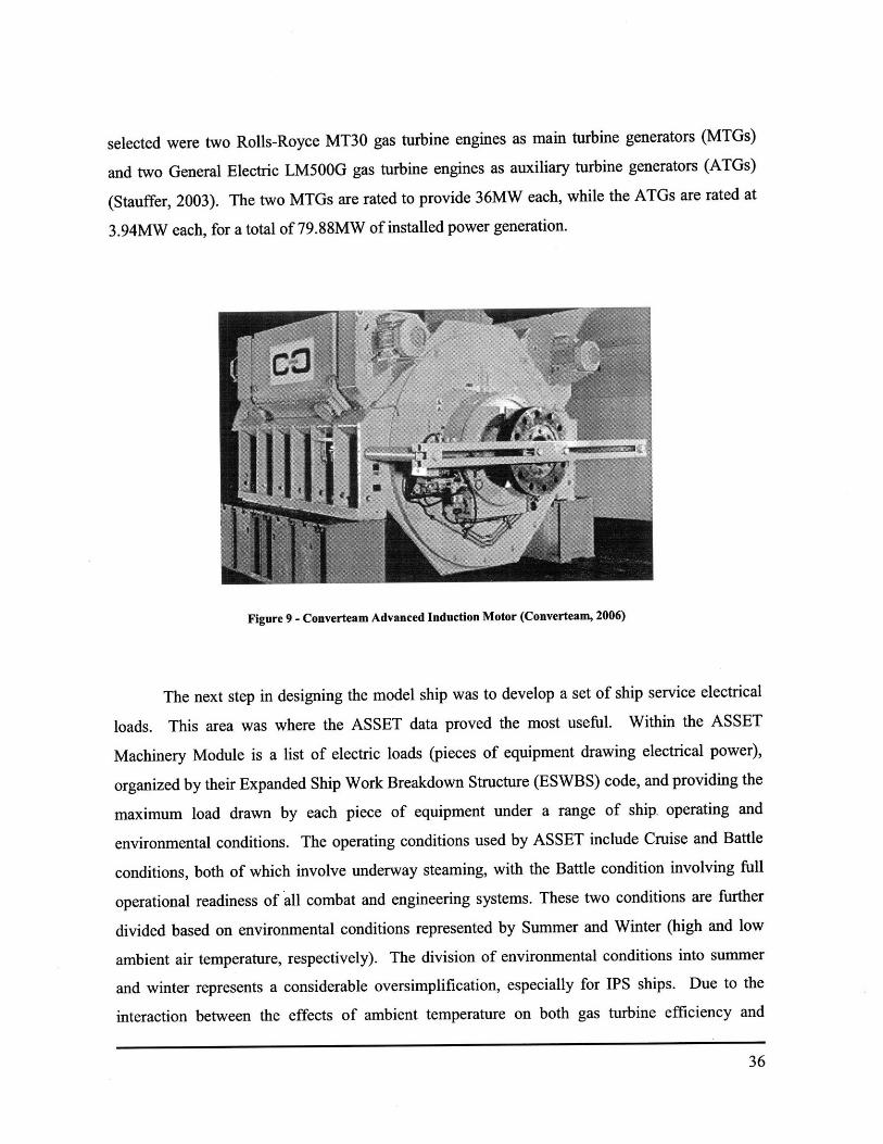
selection was simplified by the fact that the Navy had already chosen and announced the
Converteam (formerly Alstom) Advanced Induction Motor (AIM), shown in Figure 9, as the
propulsion motor for DDG-1000. Initially a more advanced permanent magnet motor solution
had been envisioned, but technology risk led to the choice of the AIM, which is also being used
on the Daring class destroyers. The DDG-1000 AIMs will be rated at 34.6MW each. The PGM
design, which at the level of detail required by this study consisted mainly of selecting the prime
movers to be used, was also relatively simple. Based both on the engines detailed within ASSET
and also on the equipment in use at the IPS Land Based Engineering Site (LBES), the PGMs
35
selected were two Rolls-Royce MT30 gas turbine engines as main turbine generators (MTGs)
and two General Electric LM500G gas turbine engines as auxiliary turbine generators (ATGs)
(Stauffer, 2003). The two MTGs are rated to provide 36MW each, while the ATGs are rated at
3.94MW each, for a total of 79.88MW of installed power generation.
Figure 9 - Converteam Advanced Induction Motor (Converteam, 2006)
The next step in designing the model ship was to develop a set of ship service electrical
loads. This area was where the ASSET data proved the most useful. Within the ASSET
Machinery Module is a list of electric loads (pieces of equipment drawing electrical power),
organized by their Expanded Ship Work Breakdown Structure (ESWBS) code, and providing the
maximum load drawn by each piece of equipment under a range of ship. operating and
environmental conditions. The operating conditions used by ASSET include Cruise and Battle
conditions, both of which involve underway steaming, with the Battle condition involving full
operational readiness of all combat and engineering systems. These two conditions are further
divided based on environmental conditions represented by Summer and Winter (high and low
ambient air temperature, respectively). The division of environmental conditions into summer
and winter represents a considerable oversimplification, especially for IPS ships. Due to the
interaction between the effects of ambient temperature on both gas turbine efficiency and
electrical loads (for heating and cooling), the difference between conditions is not as
straightforward as standard mechanical transmission ships, which experience only engine
efficiency effects due to ambient temperature (Fireman & Doerry, 2007). Despite the flaws in
the ASSET conditions, the presence of detailed load data was too valuable to pass up. Creating
new conditions and attempting to translate the load data between them would have added another
dimension of complexity to the design process with little added value for the study. In addition
to the four conditions already mentioned, ASSET provides load data for two further conditions,
Anchor and Emergency. Anchor could stand either for a vessel literally at anchor or a vessel
inport steaming, for instance when the shore-based power supply is incompatible or inadequate.
Emergency represents a minimal power consumption condition, and could be considered to
represent a damage situation (or damage drills during normal operations).
The load data from ASSET was transferred to a spreadsheet, where the various ESWBS
load groups were evaluated for completeness. Additional loads were added within the groups to
account for equipment not included in the ASSET report, such as electric fire pumps, or to divide
systems into multiple components for placement within different electrical zones. Each load was
also assigned to one of three power types: 450 VAC, 60Hz power, the most common type of
power used in the U.S.; 450 VAC, 400Hz power, used in special applications such as radar,
helicopter support, and missile systems; and 650 VDC power, which is only one of several DC
voltages used aboard ships, but was chosen to represent all of them for simplicity. Various types
of DC motors and resistive heating units use DC power, represented in this model by 650 VDC.
Load values were based primarily on the ASSET data where possible, with other values based on
engineering judgment and the author's experience onboard a U.S. Navy destroyer. The exact
values and descriptions of the loads were not critical for this study. Instead it was desired to
have a sufficiently large number of loads, requiring multiple types of power, and distributed
evenly throughout the ship.
Once the load list was created, the loads were then placed into six zones within the ship.
This number of zones was chosen both as representative of a likely IPS design and also based on
conversion gear capacities, which will be discussed later. Originally a three zone configuration
was considered for simplicity, but capacity issues, a desire for realism, and the minimal impact
of zone quantity on simulation complexity and processing time led to the increase.

Consideration was given to logical zonal placement of equipment, based on likely location
within the ship, collocation for related systems, and survivability for distributed systems.
In addition to zonally dividing the loads, further additions were necessary to the load list.
The ASSET loads provided were the maximum load for each piece of equipment for each
condition, and were intended to be used for power system design and component sizing. Toward
this end, the maximum load for all conditions for each piece of equipment was determined and
compiled for use in designing the power system. The resulting maximum margined ship service
load was 13.76 MW. While the maximum loads are useful for design, these values are of limited
use in modeling operations, where loads may only draw a fraction of their maximum load or may
only operate a portion of the time. To address this, an operational load factor was assigned to
each load. This factor was a value between 0 and 1 (the actual maximum was 0.99) and
represented the portion of time that each load would draw its conditional load. While this factor
does not completely represent a variable load over variable periods of time, it was adequate for
the purpose of this study. Another crucial area not addressed by the ASSET data was QOS.
Each load was assigned to one of the three QOS load categories (UI, STI, LTI), based primarily
on engineering judgment and also the need to have a reasonable number and distribution of each
of the categories throughout the ship. The final load list of 193 ship service loads, including the
load nodes discussed later in this chapter, can be found in Appendix I - Ship Service Electrical
Loads.
The final step in designing the ship was to create a simulated mission profile for the
model. It was deemed undesirable to fix the duration of the mission at this stage in the model
development, so the profile was developed using percentages of operating time. The profile
consisted of two primary factors, the operating condition and the propulsion motor module
loading, as derived from vessel speed. The operating conditions chosen were those used by
ASSET, discussed above. Within the constraints of the ASSET operating conditions, the total
time was allotted as shown in Table 1, with roughly two-thirds of underway time spent in the
cruise condition, divided equally between summer and winter, while summer and winter battle
conditions accounted for one-third of underway time. Time at anchor and inport was allotted
one-tenth of the total mission time, which translates to 18 days for a typical six-month
deployment. This was considered a reasonable amount for several portcalls as well as refueling

and replenishment stops. This mission profile was meant to address a single continuous
deployment, as opposed to a longer period of normal vessel operations including time spent in its
homeport. This could be included in future versions the model, but was not done in this study to
avoid the added complications of modeling shore power and the impacts on vessel operations of
timing within the inter-deployment training cycle.
Table 1 - Operating Conditions
In addition to allotting time to each operating condition, the mission profile also includes
PMM loads. These loads are dependent primarily on the ordered speed of the vessel, although
other factors due come into play. The efficiency of the PMM varies based on loading. For the
Converteam AIM, efficiency of roughly 97% is achievable above 80% loading, decreasing to as
low as 80% efficiency at 20% loading and below (Hodge & Mattick, 2000). Additionally there
is the option to use only a single shaft at lower speeds. This is commonly done on mechanical
drive ships to conserve fuel, but this benefit does not translate directly to IPS. There are reasons
for single shaft IPS operation, however, including running one PMM at a higher loading (and
thus greater efficiency than two PMMs) or the need to conduct maintenance on one shaft.
To calculate the required PMM loads, it was first necessary to determine the speeds to be
examined. The potential speeds of the vessel were grouped into seven bins based roughly on the
concept of engine bells. Each bell group was then given a representative speed, which was
compared to the DD(X) speed-power curve data generated by ASSET. Based on this data, a
spreadsheet program was used to calculate the PMM loading necessary for each speed,
accounting for variations in efficiency based on loading and number of shafts. The PMM loads
calculated in this manner are given in Table 2.
Operating Condition Time FractionSunmer Cruise 30%Winter Cruise 30%Sunmer Battle 14%Winter Battle 14%Anchor 10%Emergency 2%

Table 2 - Speed-Derived PMM Loads
Within the time allotted to each operating condition, it was also necessary to assign each
of the speed-derived PMM loadings a percentage of time. Since the ship does not use propulsion
loads at Anchor, and ambient temperature has no discernable effect on propulsor or PMM
efficiency, only three different conditions, Cruise, Battle, and Emergency needed to be
considered. Based to some extent on the work of Surko and Osborne (2005) as well as the
author's destroyer experience and engineering judgment, the time factors for each speed were
determined for each operating condition, and are given in Table 3.
Total PMM Load [KW]Condition Bell No. % of time 2 PMM I PMM
2 5% 0 03 40% 1730 1903
Cruise 4 20% 2595 28555 25% 6055 66616 10% 13840 130962 5% 03 25% 17304 20% 2595Battle5 20% 60556 15% 138407 15% 677731 20% 0 02 15% 0 03 30% 1730 19034 15% 2595 28555 5% 6055 66616 15% 13840 13096
Table 3 - PMM Loads by Operating Condition
'40
Bell No. Speed %ofMax Both PMM Single PMM[Ikt] PMM Load PMMI [KW] PMM2 [KW] [KWJ
Off 1 0 % 0 0 0All Stop 2 0 0% 0 0 01/3 3 5 2% 865 865 19032/3 4 10 3% 1298 1298 2855Standard 5 15 7% 3028 3028 6661Ful 6 20 16% 6920 6920 13096Flank 7 30 95% 33887 33887 NIA
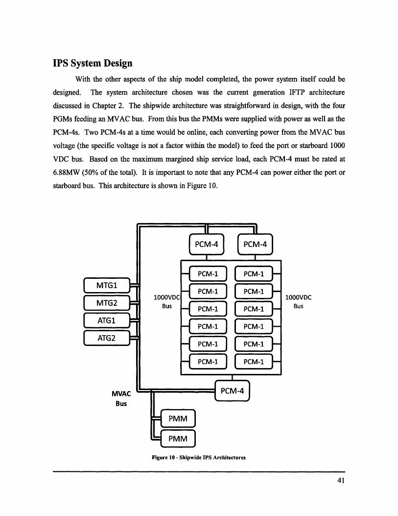
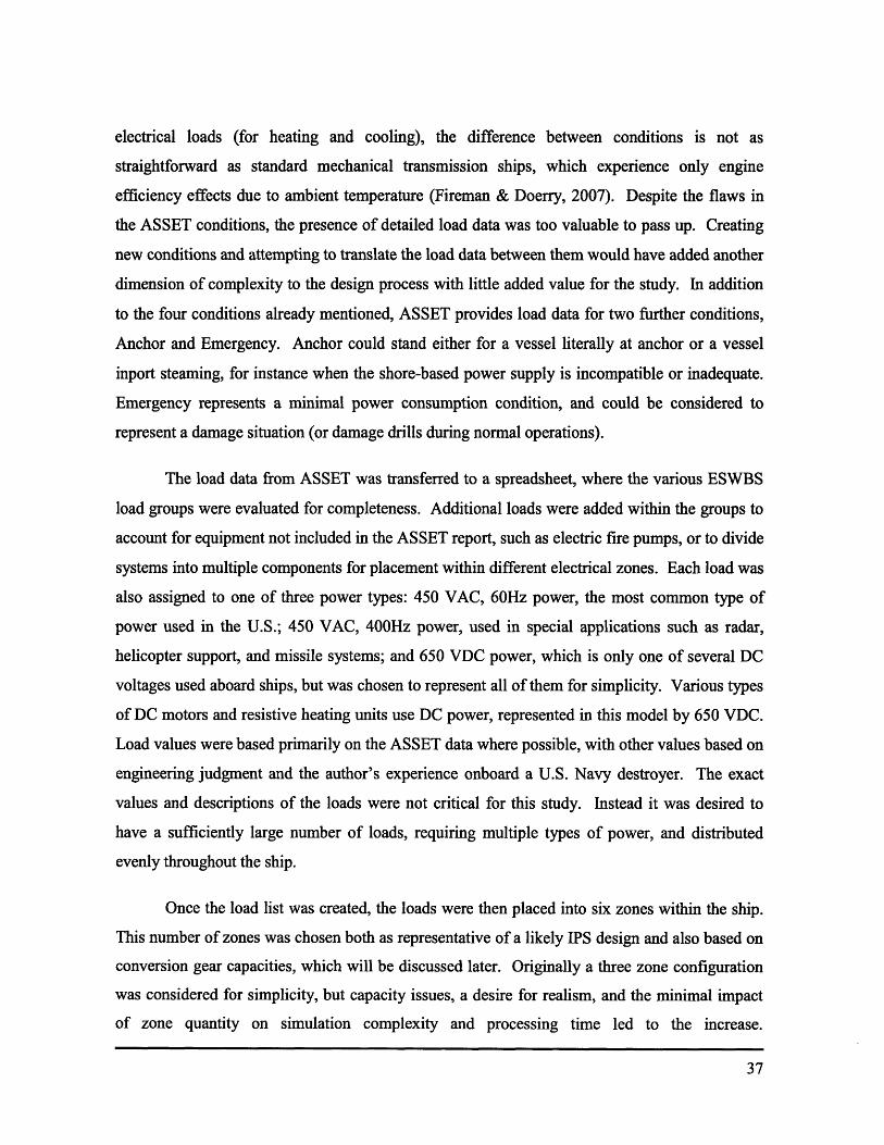
IPS System DesignWith the other aspects of the ship model completed, the power system itself could be
designed. The system architecture chosen was the current generation IFTP architecture
discussed in Chapter 2. The shipwide architecture was straightforward in design, with the four
PGMs feeding an MVAC bus. From this bus the PMMs were supplied with power as well as the
PCM-4s. Two PCM-4s at a time would be online, each converting power from the MVAC bus
voltage (the specific voltage is not a factor within the model) to feed the port or starboard 1000
VDC bus. Based on the maximum margined ship service load, each PCM-4 must be rated at
6.88MW (50% of the total). It is important to note that any PCM-4 can power either the port or
starboard bus. This architecture is shown in Figure 10.
1000VDCBus
Figure 10 - Shipwide IPS Architectures
The in-zone architecture of the system is shown in Figure 11, and this is where most of
the power system design work was required, as the number and type of converters required
differed from zone to zone. Again following the IFTP architecture, with each zone there are two
PCM-ls, one per 1000 VDC bus. The PCM-ls each contain a number of SSCMs, converting
power to either 650 VDC (the generic DC voltage used by DC loads within the model) or 800
VDC. From the PCM-1, the 650 VDC power goes directly to its PDM, with a cross-connect
(most likely auctioneering diodes) joining the SSCMs from the two PCM-ls. The 800 VDC
power from each PCM-1 is then routed, again via auctioneering diodes to the single PCM-2
within the zone. The PCM-2 contains a number of SSIMs to convert the 800 VDC power to 450
VAC, at either 60Hz or 400Hz. The 400Hz and 60Hz AC power is then fed to its respective
PDM, which represents the necessary switches and load centers required for distribution.
Figure 11 - Zonal IPS Architecture
Within each zone the number of conversion or inversion modules required was dictated
by the quantity of each load type present in the zone. Each SSCM or SSIM was considered to
have a capacity of 300KW, with a maximum of 10 modules per PCM-1 or PCM-2 (Hiller, 2003).
The zonal loads were tabulated and sorted to determine the total load for each type of power and
then for each QOS category within the types. These load totals were then increased by a 30%
margin factor. To ensure adequate supply in the event of a SSCM/SSIM failure, an N+1
redundancy scheme was employed. Using this approach, the total capacity required for each
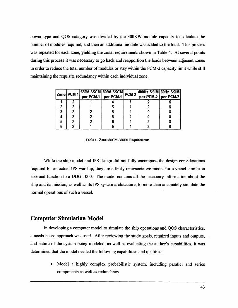
power type and QOS category was divided by the 300KW module capacity to calculate the
number of modules required, and then an additional module was added to the total. This process
was repeated for each zone, yielding the zonal requirements shown in Table 4. At several points
during this process it was necessary to go back and reapportion the loads between adjacent zones
in order to reduce the total number of modules or stay within the PCM-2 capacity limit while still
maintaining the requisite redundancy within each individual zone.
Table 4 - Zonal SSCM / SSIM Requirements
While the ship model and IPS design did not fully encompass the design considerations
required for an actual IPS warship, they are a fairly representative model for a vessel similar in
size and function to a DDG-1000. The model contains all the necessary information about the
ship and its mission, as well as its IPS system architecture, to more than adequately simulate the
normal operations of such a vessel.
Computer Simulation Model
In developing a computer model to simulate the ship operations and QOS characteristics,
a needs-based approach was used. After reviewing the study goals, required inputs and outputs,
and nature of the system being modeled, as well as evaluating the author's capabilities, it was
determined that the model needed the following capabilities and qualities:
Model a highly complex probabilistic system, including parallel and series
components as well as redundancy
Z650V SSCM 800V SSCM 400Hz SSIM 60Hz SSIMZone PCM-1 PCM-2eper PCM-1 per PCM-1 per PCM-2 per PCM-21 2 1 4 1 2 62 2 1 5 1 2 83 2 2 5 1 0 84 2 2 5 1 0 85 2 2 6 1 2 86 2 1 5 1 2 8

* Model multiple random failures with cascading system impacts
* Model the system behavior over small increments for very long periods of time
* Accept a large number of input variables
* Run in an accessible, user-friendly environment
* Facilitate early and frequent code testing and debugging
The first feature to be determined was the modeling technique to be applied. The first
two needs presented a problem for most traditional analytic reliability modeling techniques. The
complexity of the power system and random nature of the failures pointed to Monte Carlo
Simulation as an obvious solution. Monte Carlo Simulation takes its name from the casino
district in Monaco, and is characterized by repeated evaluation of a system model using random
values of the system parameters according to a desired probability distribution. The primary
benefit of Monte Carlo Simulation is that it avoids complex mathematical analysis of the system.
Provided the model adequately simulates the system's behavior, Monte Carlo Simulation can,
over a sufficiently large number of runs, reveal important behavioral trends that would be
prohibitively difficult to determine through traditional analytic methods. The primary drawback
to this technique is its costly use of computer processing time, due to the large number of runs
required to effectively discern system trends (O'Connor, 1991, pp. 142-143).
The next feature to be addressed was the software environment. Based first on
accessibility, three main options presented themselves, Microsoft Excel, MATLAB, and
MathCAD. MathCAD was eliminated quickly due to unfamiliarity with its Monte Carlo
capabilities and previous difficulties writing and debugging complex programs within the
software. Excel was the most familiar program, with well documented Monte Carlo Simulation
capabilities, but a spreadsheet approach was considered too tedious for modeling the extreme
complexity of the potential system interactions. This left MATLAB, which was less familiar
than Excel, but possessed the most documentation and was considered to be the simplest method
for implementing the complex IPS system. In the end MATLAB was selected, but used in
tandem with Excel. Any manipulation that could be accomplished outside of the MATLAB code
helped to simplify the model, and Excel was used extensively for this purpose. This dual
environment approach also facilitated the input of large numbers of variables.

The remaining needs had to be addressed by the architecture of the simulation model
itself. In order to facilitate testing and debugging early and often, a modular approach was
decided upon. The code would be built in pieces as separate m-files (MATLAB code files) that
would be called as functions by a master module. Each piece would accomplish a specific
function within the model and the information passed between modules would be minimized and
standardized as much as possible. The standardization was accomplished together with the need
for analysis of small increments over a large time period. By establishing the simulation
timeframe and desired increment upfront, all information passed between modules could be set
to a standard array size (the total number of increments), which would help to eliminate data
mismatch issues and simplify validation of individual modules. It also ensured that the model
was optimized to function over a large time period. If a module functioned poorly (i.e. slowly)
for the desired number of increments, it could be evaluated and measures taken to enhance its
performance. This ultimately proved to be a major factor in the time required to build the model,
but at the same time was essential for its successful function.
Within the overall program, the code was broken into modules according to its function.
Early in the program design, the need for certain functional modules became apparent. A
module to generate randomly sequenced ship missions of a given duration and according to the
mission profile was clearly needed, and would provide the basic inputs for most of the other
modules. A module to generate the actual loads for each time increment was also needed. A
module to generate and evaluate the impacts of power system failures was another necessity. As
program development progressed, the need for additional functional modules arose. These
included a new module for addressing only PGM loads and splitting the power system evaluation
module into two, one to generate the failures and another to evaluate their impact on the power
system. In addition to addressing the functional modules, it was necessary to minimize the
impact of loading inputs and compiling the ultimate output data on the model's performance.
This was accomplished through a master module, which called the submodules as functions
within its routine, while taking care of loading a few large input arrays and compiling and saving
the output data separately from the system evaluation performed by the submodules. The final
program architecture for the functional modules is shown in Figure 12, and is followed by
descriptions of the individual modules as well as the master module. Information passed
between modules is indicated in brackets and located along the path it travels, while inputs and
45
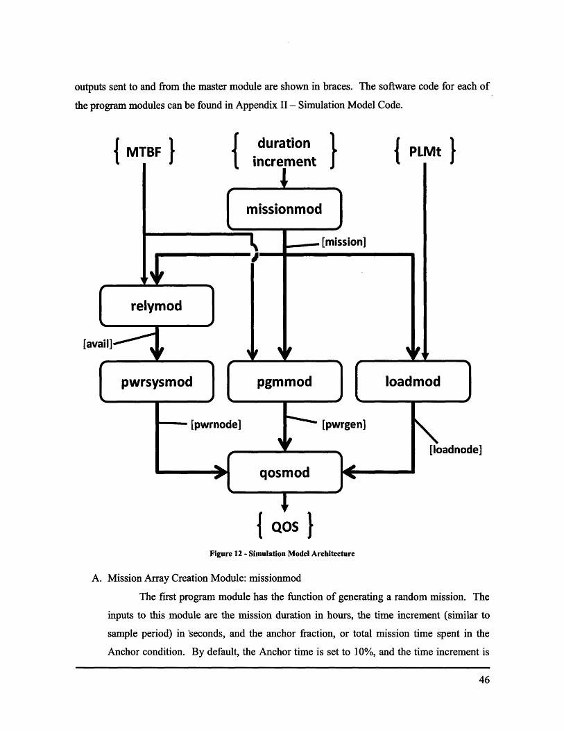
outputs sent to and from the master module are shown in braces. The software code for each of
the program modules can be found in Appendix II - Simulation Model Code.
jMTBFI I U'duration PLMtMTBF PLMtI?
J
Figure 12 - Simulation Model Architecture
A. Mission Array Creation Module: missionmod
The first program module has the function of generating a random mission. The
inputs to this module are the mission duration in hours, the time increment (similar to
sample period) in 'seconds, and the anchor fraction, or total mission time spent in the
Anchor condition. By default, the Anchor time is set to 10%, and the time increment is

set to 300s (5 minutes). After reviewing the input variables and default values, the
module generates a random sequence of operating conditions, each lasting for one hour of
the mission duration. The conditions are numbered one through six, corresponding to the
ASSET operating conditions as listed in Table 1, and are governed by the time fractions
given in the table as well. However, condition five, representing Anchor, is not included
at this point. This is addressed in the next program process, which randomly inserts full
24 hour blocks of time in the anchor condition (1 day is assumed to be the smallest unit
of time the ship will spend in this condition), up to a maximum number of days governed
by the anchor fraction described above. The next process enforces the constraint that the
ship will not switch directly between summer or winter temperature conditions, although
it can switch between cruise and battle conditions within the same temperature condition.
Up to this point the function has been operating on loops or vectors of length = duration.
The next process expands the existing operating condition vector to its full length and
final form, a column vector of length = the total number of time increments in the
mission, which is named opcon.
Once the operating conditions have been established, the second half of the
mission module generates random PMM loads at each time increment according to the
assigned operating condition and governed by the time fractions and loads given in Table
3 for each condition. The final process collects the incremental load data into a column
vector named pmm. The opcon and pmm vectors are then merged into the module's
single output variable, a two column array of length = total increments named mission. It
is important to note that efforts were made to utilize only standard MATLAB built-n
functions, such as rand.m, which generates a uniformly distributed random number.
This applies to all modules of the simulation model. One notable exception is the use of
the randint.m function in the anchor insertion process. This function resulted in a slight
time savings per run which is then magnified by the large number of runs required for
Monte Carlo Simulation.
B. Power Load Array Creation Module: loadmod
The second program module has the function of generating the individual PLM
loads required for each increment of the mission. It takes as inputs the mission array
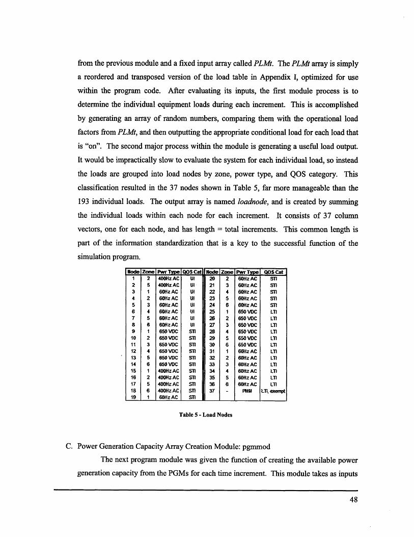
from the previous module and a fixed input array called PLMt. The PLMt array is simply
a reordered and transposed version of the load table in Appendix I, optimized for use
within the program code. After evaluating its inputs, the first module process is to
determine the individual equipment loads during each increment. This is accomplished
by generating an array of random numbers, comparing them with the operational load
factors from PLMt, and then outputting the appropriate conditional load for each load that
is "on". The second major process within the module is generating a useful load output.
It would be impractically slow to evaluate the system for each individual load, so instead
the loads are grouped into load nodes by zone, power type, and QOS category. This
classification resulted in the 37 nodes shown in Table 5, far more manageable than the
193 individual loads. The output array is named loadnode, and is created by summing
the individual loads within each node for each increment. It consists of 37 column
vectors, one for each node, and has length = total increments. This common length is
part of the information standardization that is a key to the successful function of the
simulation program.
Node Zone Pwr Type QOS Cat Node Zone Pwr Type QOS Cat1 2 400Hz AC Ut 20 2 60Hz AC ST12 5 400Hz AC U] 21 3 601iz AC Snl3 1 60Hz AC U1 22 4 6O1z AC STI4 2 60iz AC UI 23 5 60Hz AC STI5 3 60Hz AC UI 24 6 60Hz AC STI6 4 60Hz AC Ut 25 1 650 VDC LTI7 5 60HIzAC UI 26 2 650 VDC LTi8 6 60Hz AC WL 27 3 650 VDC LTI9 1 650 VDC STi 28 4 650 VDC LTI10 2 650 VDC STI 29 5 650 VDC LTI11 3 650 VDC 1sn 30 6 650 VDC LTI12 4 650 VDC ST1 31 1 60Hz AC LTI13 5 650 VDC ST 32 2 60z AC LTI14 6 650 VDC T51 33 3 601HzAC LTi15 1 400Hz AC ST 34 4 6Oiz AC LTI16 2 400Hz AC ST 35 5 60flz AC LTI17 5 400Hz AC STI 36 6 60Hz AC LTI18 6 400Hz AC ST 37 - PMM LTI, exempt19 1 601HzAC ST ,
Table 5 - Load Nodes
C. Power Generation Capacity Array Creation Module: pgmmod
The next program module was given the function of creating the available power
generation capacity from the PGMs for each time increment. This module takes as inputs

the mission array from the first module and the array MTBF, generated by the master
module. After evaluating its inputs, the first process is to set the PGM availability
constants MTBF and MTTR. The MTBF is a variable from the input MTBF, while the
MTTR was set within the module to a default value of 5 hours. The next process is to set
an operating array for the PGMs. This array is based on the incremental condition, and
consists of binary column vectors specifying whether each of the four prime movers is
operating for each increment. A notable simplification at this step is the lack of
distinction between the individual PGMs. While the code allocates a number of each
type of engine based on the operating condition, it does not specify which specific engine
is operating (MTG1 vs. MTG2, for instance). Given the complex issues involved with
choosing which engine is online, addressing this decision would have involved
considerable additional coding time and potential increases in processing time for little
added value to the model.
Once the array of PGM operation has been created, the next process is to generate
the random engine failure and repair times. This is done by generating arrays of random
numbers, limited in length to a reasonable maximum number of failures per engine (10 in
this case, which statistically should almost never occur within a six month duration). The
failure and repair times are both exponentially distributed, using the means generated
earlier, and are then combined to insert engine downtimes (binary zeros) into the PGM
operation array. The next process involves detecting these random downtimes and
bringing the appropriate standby PGMs online by the next increment (5 minutes is a
reasonable timeframe to bring a standby turbine generator online). Once the standby
generator operations have been inserted, the binary matrix is multiplied by the PGM
ratings and then summed for each increment. This results in the output array pwrgen,
which is a column vector of the standard length containing the total power generation
capacity available for each increment.
D. Power System Availability Array Creation Module: relymod
This program module has the function of randomly generating the availability of
each element of the power system for each time increment. It takes the inputs mission
and MTBF. From MTBF it creates an array of failure times, one for each system element.

Two notable simplifications take place at this phase. First, each element has only one
failure time during the mission. This was done to save processing time due to the low
likelihood of multiple failures per element during the mission. While a certain number of
elements would certainly fail multiple times during a mission, the element MTBFs being
examined were all an order of magnitude greater than the mission duration, and it was
determined that the added complexity was of limited value for this study. This does not
hold true for the PGM failures (based on their considerably lower MTBF), and explains
why separate modules were used to evaluate the PGMs and the remaining power system
failures. The second simplification is a fixed repair time, set at 5 increments in this case.
Again, this simplification was used to reduce processing time, by assuming all repairs
take exactly the MTTR to conduct, instead of using the MTTR to model repairs
probabilistically. Once the failure times are generated, they are combined with the fixed
repair downtime and inserted into an binary array of ones having the standard length and
containing a column for each system element (171 columns). This array is the module
output avail.
E. Power System Operational Evaluation Module: pwrsysmod
This program module has the function of evaluating the effects of element failures
on the available power delivered to the loads by the power system. The input to this
module is the avail array from the previous module. After evaluating the input, the first
process is to account for PCM-4 failures and their impact on the system (through the loss
of the port or starboard bus). These bus failures are then inserted into a column vector
which gives the total bus power available for each increment and is stored in the last
column of the module output array pwrnode. This array has standard length and contains
a column for each load node fed by the power system plus the bus power column
mentioned above.
The remainder of the module evaluates the power system within each zone. First
the available total capacity is determined for each type of SSCM within each of the zonal
PCM-ls, based on SSCM and bus failures. From the available 800 VDC SSCM capacity,
the available SSIM capacity is determined. The power available at each node within the
zone is then determined by multiplying the availability of the respective node PDM with

the appropriate available SSCM/SSIM capacity and storing this value for each increment
in the appropriate nodal column of pwrnode. This process is then repeated for the
remaining electrical zones. This module simplifies the power system by limiting the
evaluation to high level components only and ignoring switching failures. The decision
to ignore these elements was made again for complexity and processing time
considerations, as this module already involves over 80% of the overall processing time
required by the simulation model.
F. Quality of Service Failure Evaluation Module: qosmod
The final program module has the function of evaluating the performance of the
power system and determining when and where QOS failures occurred during the
simulated mission. The module takes the arrays loadnode, pwrnode, and pwrgen as
inputs from the modules preceding it. The first process is to manipulate the input arrays
to create two arrays for comparison. The nodal loads are summed for each increment and
subtracted from the available PGM capacity to give the available power at the PMM node
and inserted into the final column of pwrnode, while the QOS exempt portion of the
PMM load in the final column of loadnode is removed. These actions result in two
arrays of identical dimension which represent the power delivered to the nodes and the
power required from the nodes, respectively. The module then simply compares these
values to determine if a QOS failure has occurred. Due to the 5 min increment time, UI
and STI nodes are considered QOS failures at any increment where power required is
greater than power available, while LTI loads require 2 subsequent increments to cause a
QOS failure. The output of this module is the array QOS, where the first column is the
increment and the second the node for each QOS failure. Because the number of failures
is not fixed, QOS has variable length.
G. Master Simulation Module: Monte XX
The master module performs all operations required for a single Monte Carlo
Simulation trial (the specific trial within an experimental set is indicated by the number
XX). Its first process is to call the static input files PLMt and MTBF XX, and store them
in its workspace to act as inputs for the function modules. The number of simulation runs

to be conducted is also determined at this point. The number of runs selected for Monte
Carlo Simulation is a prime determinant of the simulation's accuracy, however this is a
square relationship, and thus the return on more runs is diminishing. An experiment was
conducted to evaluate the number of runs required by running the model for 10, 50, 100,
500, and 1000 runs and then evaluating the standard error of the results. While the results
improved as runs increased, the improvement diminished considerably when compared to
the great increase in run time. For this reason the number of runs was capped at 1000 to
maintain a reasonable amount of processing time per trial while still gaining acceptable
accuracy. The only remaining input necessary for the module was the mission duration.
For this study the duration was selected as 4,380 hours, which equals six months, the
length of a nominal overseas deployment. This duration also represented a reasonable
timeframe to examine from the standpoint of failure data and processing time, resulting in
52,560 total increments to examine given a five minute increment length. While Doerry
and Clayton (2005, p. 4) propose 30,000 hours (3.4 years) as a reasonable target QOS
value (although they are referring to individual load QOS), due to the processing time
required and the fact that this study does not examine shorepower or homeport
conditions, a six month deployment was selected as the duration.
The central process of the master module is to call the functional modules in a
loop for the desired number of simulation runs. In addition to calling these six functions,
it also collects necessary data from each run within the loop. This includes collecting the
QOS output array as well as calculating the increment of the first failure and the total
number of failures for each run, and repeating these calculations while excluding QOS
failures at the PMM node. Once the looped runs are complete, the module then computes
the mean values of these failure characteristics for the entire trial. It also calculates the
number of failures for each node and the percent of the total failures that occurred at that
node during the entire trial. The final process is saving these trial output values in a file
named Data_XX so that they can be compared between different experimental trials.
Design of ExperimentsWith the simulation model complete, the remaining item to address was the treatment of
component reliability as a variable. In order to examine the effects of changes in individual
component reliability on the overall system, the reliability (in the form of component MTBF)
would have to be varied for each component and an individual Monte Carlo trial (1000 runs)
conducted. In examining the power system, no fewer than 13 different types of components
existed, and each should be considered over a range of MTBF values. Assuming simply a high
and a low value were considered for each, 213, or 8,192 trials would need to be conducted. For
three MTBF levels per component the number of trials increases to 1.6 million! At over 1 hour
of processing time per trial, this sort of analysis was not possible. Clearly an experimentation
plan was needed to reduce the number of trials while still capturing the effects of changes in
reliability on QOS performance.
This sort of difficulty is common in engineering problems and is addressed by a concept
called Design of Experiments (DOE). The basic purpose of DOE is to determine the relationship
between the factors affecting a system or process and its output, while minimizing the number of
experiments necessary to effectively determine these relationships. There are numerous
techniques that fall within the realm of DOE, including fractional factorial design, response
surface methodology, Taguchi methods, robust parameter design, and many others (Wu &
Hamada, 2000). It was not the goal of this study to examine their individual merits, however,
and so for the experimental design the JMP statistical software program was employed. Using
the JMP DOE platform, the 13 component types were entered as factors and given three nominal
levels of reliability. Based on the inputs given to the program an experimental trial plan was
recommended. This plan was an array giving the level to be used for each of the 13 components
in each trial. The final array selected was based on a Taguchi L27 orthogonal array, but with the
addition of 2 extra trials to add a center point and opposite corner point to the experiment. The
final experimental design consisted of 29 total trials (L27 is named for the number of trials)
shown in Table 6. As the MTBF values were not known, all electrical components were given
three basic levels, 10,000, 20,000, and 30,000 hours, while the PGMs were assumed to have
much lower MTBFs with the levels 1,000, 3,000, and 5,000 hours. These values were chosen
primarily to ensure a measureable number of failures occurred within the mission duration, and
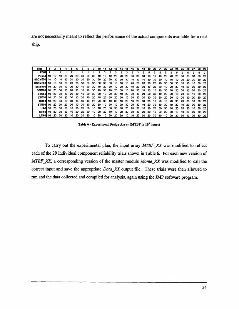
are not necessarily meant to reflect the performance of the actual components available for a real
ship.
Trial 1 2 3 4 5 6 7 8 9 10 11 12 13 14 15 16 17 18 19 20 21 22 23 24 25 26 27 28 29PGM 1 1 1 1 1 1 1 1 1 3 3 3 3 3 3 3 3 3 5 5 5 5 5 5 5 5 5 5 3
PCM-4 10 10 10 20 20 20 30 30 30 10 10 10 20 20 20 30 30 30 10 10 10 20 20 20 30 30 30 30 20SSCM650 10 10 10 20 20 20 30 30 30 20 20 20 30 30 30 10 10 10 30 30 30 10 10 10 20 20 20 30 20SSCM800 10 10 10 20 20 20 30 30 30 30 30 30 10 10 10 20 20 20 20 20 20 30 30 30 10 10 10 30 20SSIM400 10 20 30 10 20 30 10 20 30 10 20 30 10 20 30 10 20 30 10 20 30 10 20 30 10 20 30 30 20SSIM60 10 20 30 10 20 30 10 20 30 20 30 10 20 30 10 20 30 10 30 10 20 30 10 20 30 10 20 30 20STI650 10 20 30 10 20 30 10 20 30 30 10 20 30 10 20 30 10 20 20 30 10 20 30 10 20 30 10 30 20LTI650 10 20 30 20 30 10 30 10 20 10 20 30 20 30 10 30 10 20 10 20 30 20 30 10 30 10 20 30 20UI400 10 20 30 20 30 10 30 10 20 20 30 10 30 10 20 10 20 30 30 10 20 10 20 30 20 30 10 30 20
STI400 10 20 30 20 30 10 30 10 20 30 10 20 10 20 30 20 30 10 20 30 10 30 10 20 10 20 30 30 20UI60 10 20 30 30 10 20 20 30 10 10 20 30 30 10 20 20 30 10 10 20 30 30 10 20 20 30 10 30 20
STI60 10 20 30 30 10 20 20 30 10 20 30 10 10 20 30 30 10 20 30 10 20 20 30 10 10 20 30 30 20
LTI60 10 20 30 30 10 20 20 30 10 30 10 20 20 30 10 10 20 30 20 30 10 10 20 30 30 10 20 30 20
Table 6 - Experiment Design Array (MTBF in 103 hours)
To carry out the experimental plan, the input array MTBFXX was modified to reflect
each of the 29 individual component reliability trials shown in Table 6. For each new version of
MTBF X, a corresponding version of the master module Monte_XX was modified to call the
correct input and save the appropriate Data_XX output file. These trials were then allowed to
run and the data collected and compiled for analysis, again using the JMP software program.

4
Chapter 4 - Results & Analysis
Experimental Results & Analysis
Once the experimental trials were complete, the output data from each individual output
file was compiled into a spreadsheet for analysis. The response data was collected in Table 7,
and included the following items for each trial [brackets indicate JMP response label], for the
load nodes described in Chapter 3:
1. Mean increment of first failure [FirstFail]
2. Mean increment of non-PMM failure [FirstFail noPMM]
3. Mean number of failures per mission [NumFail]
4. Mean number of non-PMM failures per mission [NumFail_noPMM]
5. Non-PMM node with highest number of failures [Mode]
6. Percent of the non-PMM failures occurring at the Mode [ModePct]
7. Percent of total failures occurring at the PMM node [PctPMM]
Because there were so many factors used and their values were set based on the experimental
array, it is nearly impossible to discern any meaningful insight from Table 7 alone. The only
item that potentially stands out is the repeated presence of several nodes as the most frequent
failure site. This can be slightly misleading, however, as in these cases a closer look at the raw
data shows that there were generally other nodes responsible for almost as many failures. This
issue will be revisited later in the discussion. Complete simulation output data can be found in
Appendix III - Simulation Output Data.

Table 7 - Collected Experimental Response Data
The most effective way to examine the experimental output was to use statistical software, for
this study JMP was chosen again, to help separate the impacts of each component reliability
factor on the system responses. After transferring the data into JMP, a model fit was conducted
for all responses and all reliability factors. The most directly useful outputs from this operation
are the JMP profiler diagrams, which are produced individually for each combination of factor
and. response. Each diagram displays the response on the vertical axis and the factor on the
horizontal. The factors consist of the component types whose MTBF values were the input
variables, while the responses are those given above. Within each diagram, the range of
response values is represented by a vertical band located at each of the three factor levels (low,
medium, and high, using the values given in Table 6). The means of each response range are
then connected by a solid line to indicate roughly the effect (or lack thereof) on the response
Trial FrstFail FirsttFai noPMM NuWmFa I umFail noPMM Made iodePct Pet PMM1 883.03 7320.27 133.60 30.03 5 4.24% 77.53%2 843.19 7160.09 13425 29.84 4 4.11% 77.77%3 904.53 10936.56 124.57 20.32 4 4.42% 83.68%4 831.64 8134.90 129.78 25.98 12 6.52% 79.98%5 836.03 5093.83 146.80 43.22 24 5.07% 70.56%6 825.92 5977.31 138.88 34.27 1 5.83% 75.29%7 839.08 7373.09 1:33.97 30.33 12 5.77% 77.36%8 878.14 6522.85 132.80 29.23 2 6.83% 77.99%9 785.99 4849.63 148.43 44.02 4 5.26% 70.34%10 853.24 6292.44 133.64 33.18 8 6.58% 75.17%It 862.93 5680.41 137.77 36.15 1 5.44% 73.76%12 814.67 6070.78 136.74 35.14 22 6.31% 74.30%13 887.56 6729.45 135,33 33.71 22 6.82% 75.09%14 870.34 5590.40 137.55 37.15 5 5.67% 72.99%15 872.58 5891.52 134.17 33.76 31 5.47% 74.84%16 850.58 6599.05 133.82 32.43 33 5.72% 75176%17 833.52 5498.64 137.41 36.95 23 6.38% 73.11%:18 878.42 6482.92 136.32 34.70 8 6.44% 74.54%19 814.75 5864.34 136.19 35.12 8 6.32% 7421%20 893.21 6335.82 133.42 33.55 24 6.53% 74.85%21 849.15 5534.28 137.23 36.39 1 5.49% 73.48%22 881.80 61468.81 133.52 33.65 31 5.49% 74.80%23 854.88 6535.33 133.68 32.83 4 7.05% 75.44%24 836.32 5556.29 136.98 37.12 23 6.35% 72.90%25 884.01 6474-54 136.08 34,98 22 6,57% 74.30%26 829.20 6099.68 134.39 33.32 32 5.63% 75.21%27 851.25 5521.93 138.54 37.07 5 5.76% 7324%28 906.07 11473.76 119.90 20.04 5 4.43% 83.29%29 889.02 7525.98 131.40 29.78 22 4.49% 77.33%
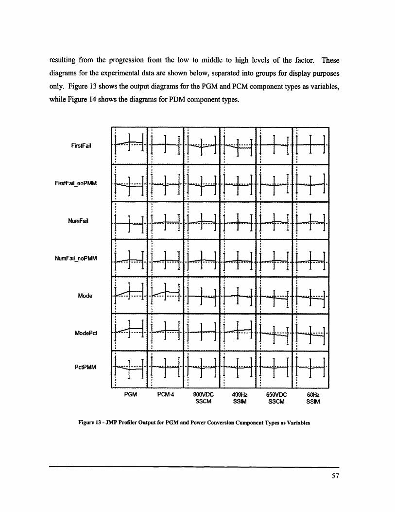
resulting from the progression from the low to middle to high levels of the factor. These
diagrams for the experimental data are shown below, separated into groups for display purposes
only. Figure 13 shows the output diagrams for the PGM and PCM component types as variables,
while Figure 14 shows the diagrams for PDM component types.
FirstFail
FirstFail noPMM
,NumFai#
NumFail noPMM
Mode
ModePct
PctPMM
4 NI alL r iE
H HtttLF~ HarF---tlt* NI Nr N I tN * i • i
F#4.. i-HiFHH i-4lHiI+i N J J :· ' c1 II ', I; I
... . I _ L _ __r1
* IN
d• 21II Ii I,
I- I( I 1a l
* Nr NL Nt Ir N
• s I• |.. ....... .. .... S . .N .I4 N S NI I-
I Nr Nr NI""I }Jitc]Lj.I at r Nr ii Na a
4 LF·l+-rr I~~JI_9~IC~ N N N 4 Ni
h·~*44+ h1H+AdF, dN Nt NI N 4N Nr N, Nr N
PGM PCM-4 800VDCSSCM
400HzSSIM
65OVDCSSCM
60HzSSIM
Figure 13 - JMP Profiler Output for PGM and Power Conversion Component Types as Variables

SNumFai noPMM
M dePct t Iit"4 i-f- FMI H-H
400 4 60Hz 654VDC 400H 4 6 4k VDC 604 I At a 4Looking first at the initial failure responses FirstFail and FirstFailnoPMM, it is clearly
less likely to be direct failure sources. In looking at the PDM components' diagrams (Figure 14),
however, a strong correlation is evident. A clear trend is shown by the consistently positive
slope of the mean connecting lines for each component. This result could also be anticipated,4·- 4 44
Lokn is a h nta faiur repns Frstai and Firsi noM ,iticlayimosil t iscrn corltiosfo thfomr Whil th PMM falrs ofun nreainsis inh Firtaldarmwe thes failue are reovd iispsbleoseiany corlain are prset Ther dontapa ob n togcreaion iheSCsSSI~s or PC-4 Thsi nupiig ie htterdnacnteeiesmkste
less ikel to b dirct filuresoures. I looing t thePDM omponnts'diagams (igur 14)howevri nPap strong creaionis evidet.Acla trend is shw ytecnisetypstv
slpeofthma conetin lie fo eac copnn.Ti resl col als be aniiptd

given that these components as modeled by the simulation are single points of failure within each
zone. Higher reliability should extend the average time before they fail, and since they are
guaranteed to cause a failure, the first instance of PDM failure will frequently be the first non-
PMM failure. The one slightly surprising result from within these first two rows of response
diagrams is the lack of a clear correlation with PGM reliability. As these items possess
significantly lower MTBFs than the electronic components, they fail much earlier and more
frequently on average. This result is useful, however, in that it could indicate that the
redundancy provided by the standby generators is adequate to prevent QOS failures arising
solely from PGM failure.
In examining the next two rows of diagrams, for the total number of failures, there is
much less of an issue with PMM failures concealing relationships. In fact the response profile
for NumFail vs. PGM component reliability actually requires the PMM failures to display a
correlation. In this case, the PGM reliability appears to have no clear impact on the total number
of power system failures shown in PGM vs. NumFail_noPMM (Figure 13), but when PMM
failures (which account for roughly 75% of failures on average according to the experimental
data) are included in the diagram immediately above, there is a clear decline in total failures as
PGM reliability improves. This indicates that most PGM failures result only in PMM QOS
failures, and their impact on the electrical system QOS is less severe. Again no clear trend
emerges from the diagrams for the power conversion components, owing most likely to
redundancy. The most interesting area is once again the single point of failure PDMs. There is a
very clear correlation between reliability and total failures, with and without PMM failures for
three components, the 60Hz STI and LTI PDMs and the 650 VDC LTI PDM. This correlation is
not surprising, as these PDMs serve the most loads, and are thus most likely to cause unmet
demands (QOS failure) when they fail. Similar, though much less pronounced effects can be
seen in the 400Hz UI and STI PDM component diagrams. What is intriguing is that there is not
a lack of correlation for the remaining components, but instead a fairly clear zero correlation.
This could indicate that these components result in such a small number of failures that
improving their reliability has almost no effect on the total number of QOS failures in the overall
system. Based on these results, if the goal is to reduce the total number of failures, clearly the
60Hz and 650 VDC PDMs should be targeted for reliability improvement.

In examining the Mode and Mode Percentage responses, there appear to be few, if any,
correlations. This is not surprising, as numerically (as opposed to qualitatively) the most
frequently occurring failure node has little significance aside from the QOS category of the node.
The mode percentage considered numerically by itself can only offer a clue to the prominence of
the most common failure node types (based on QOS and power type), since nearly all trials
displayed a consistent behavior pattern wherein similar types of nodes accounted for similar
percentages of the total QOS failures. There are two potential correlations, however, and both
exist within the redundant power conversion components. The first is a negative correlation
between the 60Hz SSIM and 650 VDC SSCM and the Mode Percentage. While this may be a
false correlation, a possible explanation is that increasing reliability in these components causes
the source of QOS failures to be more random and therefore less concentrated in nodes
downstream from these components. The other possible correlation exists between the same two
components and the mode. This result is even more difficult to interpret and may also be false,
but a possible explanation could be that increasing reliability to these components, which serve
all of the LTI and most of the STI loads could shift more failures to numerically lower nodes,
which serve STI and UI loads. One fact that disputes this explanation is that these conversion
modules also serve a majority of the UI and STI loads, indicating this relationship may not exist,
or may require a more detailed examination.
Looking at the diagrams for the percentage of failures occurring at the PMM node, there
are no apparent relationships with the reliability of the PGMs or any of the conversion module
components. This is unsurprising for the redundant conversion modules which cause few
failures, but slightly unexpected for the PGM. As discussed above, it appears as if most PGM
failures lead to PMM QOS failures, so one would expect a lower percentage of total failures to
be PMM failures if PGM reliability improves. Clear correlations do exist, however, between the
percentage of failures occurring at the PMMs and the reliability of the PDMs. As before these
relationships are less pronounced for the PDMs that are less prevalent (and therefore result in
fewer total failures), while the improving reliability for the PDMs which cause the most failures
greatly increases the percentage of total failures occurring at the PMMs. This result helps to
confirm the earlier indications that improving the reliability of the highly loaded PDMs first
would have a more significant positive effect on system QOS.

5
Chapter 5 - Evaluation & Conclusions
Model Evaluation
The results from this study demonstrate the potential benefits of this approach to
modeling IPS systems and QOS. While certainly not conclusive, this analysis indicated or
validated several key correlations between reliability and QOS performance that may not have
been anticipated without the use of modeling. The model effectively performed its purpose of
simulating the QOS performance of a given system architecture over the length of a mission. It
allowed the examination of a key unknown, reliability, to be conducted for a range of
components and displayed the influence of these variables on the overall system. Most
importantly, the model accomplished these tasks in a straightforward and relatively expedient
manner, a necessity for any early stage design tool.
While the simulation model generally fulfilled its objectives, it has several weaknesses
and limitations. Many simplifications were required to reduce the complexity of the program
code and minimize the processing time required. The current model only includes the highest-
level elements of the power system, and even many of these were left out or assumed away. This
resulted in a model that, while sufficient for a study of this narrow scope, would require
considerable modification and improvement to be a truly useful IPS design tool. A more realistic
model would need to include considerably more components and model their interdependencies
in a much more sophisticated manner. It would also most likely be expected to model the
individual PGMs and PMMs and their components, instead of treating them as identical,

monolithic entities that function as "black boxes".. The manner in which component failures and
repair are treated would also require considerable improvement. Instead of single failures and
fixed repair times, the power system components should be modeled in a manner similar to the
PGM availability module, where both failure and repair are modeled as random events that can
occur multiple times. It would also be better to get away from the constant failure and repair rate
assumptions, and instead model the failure and repair behaviors using more advanced probability
techniques, such as the multi-parameter Weibull distribution. In the extreme, preventative
maintenance and less-than-perfect repairs could also be modeled. A final area for improvement
would be the experimental design and data analysis. These areas were not the main focus of this
study, and were handled rather simplistically. To be of real benefit, the Design of Experiments
would have to be conducted in a much more thorough manner. The data analysis also requires
improvement, primarily in terms of the chosen response variables. While these responses
seemed to be reasonable measures of system QOS performance, most were interconnected or
difficult to evaluate numerically. These complications limit the confidence one can place in any
conclusions drawn from the data analysis. Any of these changes would have a significant impact
on the complexity and performance of the model, but most of them are necessary to make it a
useful tool for examining future IPS designs.
Despite these limitations, the simulation model has many positive attributes that argue for
its continued use in future applications. The most important of these is its modular architecture.
This allows different facets of the program to be improved or expanded independently as the
program is tailored to the specific needs of the user, and also facilitates testing and debugging.
The standard inter-module array length is also a benefit for improvement and testing of the
model. Another important asset is the ability to run within the MATLAB environment. This
software is among the most commonly available numerical tools, and a significant proportion of
design engineers possess at least a basic familiarity with its use and programming techniques.
This feature represents considerable value, in that the module is essentially an open-source,
open-architecture application, which can be used by nearly anyone and freely and readily
adapted for each user's specific needs.
The capabilities of individual users or user groups also significantly impact the model's
effectiveness. Access to more powerful computing resources would allow the number of runs to

be increased sufficiently to realize noticeable benefits in the variance of the output data. This
could greatly reduce the uncertainty involved in the data analysis and allow detection of smaller
effects that might otherwise go unnoticed. Greater processing power would also allow more
complex models to be examined, and possibly over longer periods of time, again increasing the
model's usefulness. The level of access to system and component data is also a major
determinant of the model's utility. If the system architecture and operating characteristics are
known accurately, then many simplifying assumptions can be avoided; and likewise if the
components are more thoroughly known. Any data that is known for certain allows the user to
examine and evaluate the unknowns with much higher granularity. This can result in more
valuable insights into the power system and its constituents.
Applications of the Model
The approach taken in this study is merely one application for this IPS simulation model.
In this case, the ship characteristics and system architecture were created based on the best
available information, experience, and engineering judgment. Even less was known about the
components that made up the integrated power system. A model that is still useful under these
conditions has great potential for use in applications involving less uncertainty.
One such application would be to conduct a more focused version of a reliability
improvement study. For a known ship and system architecture, component reliability could
again be treated as a variable. Assuming, however, that the current system components and their
reliability characteristics were known, the study could be used to target areas for improvement.
First the system in its current configuration would be modeled and repeatedly simulated to
establish a solid baseline. Design of Experiments principles would then be used to develop a test
plan for systematically evaluating improvements in individual components to determine which
components or combinations of components produced the greatest improvement in QOS
performance. These components could then be upgraded (if better components exist) or
development work could be commenced to improve them. Conversely, a cost reduction study
could be conducted along the same lines, but instead looking for the components that had the

smallest influence on system QOS. These components could then be swapped for less reliable
(and presumably less expensive) versions.
Another application for this type of model would be an analysis of alternative system
architectures. Assuming a fixed set of available components with known reliability
characteristics (although due to the model's flexibility the fixed requirement is not a necessity),
the model could be used to simulate the performance of various modifications to the power
system architecture and analyze their influence on QOS performance. Similarly, the effect and
importance of component redundancy within a system architecture could be explored by
evaluating QOS for different levels of redundancy or alternative redundancy schemes. These
studies could again be targeted either at improving performance or maintaining a minimum
performance threshold while reducing costs.
A third possible application could involve modifying the model to examine a different
concept of Quality of Service. By modifying the node assignment scheme and changing aspects
of the QOS evaluation module, the model could be used to simulate a ship's performance in
terms of mission system QOS, where loads are grouped by their function within the overall ship
mission (e.g. air defense mission loads) and QOS is defined not by the delivery of power to
individual loads, but instead by the continued ability of the ship to complete its individual
missions. Once again the objective could be either performance or cost-centric. This type of
analysis could be especially useful in further developing the concept of a "high-low mix" of
warships possessing varying levels of capability and survivability for similarly differing levels of
cost. Other potential QOS concepts could include an increased focus on the traditional definition
of power quality, which is essentially avoided in the current model. This type of approach would
most likely require significant modification to most of the modules, or perhaps even the addition
of one or more modules to account for the new factors involved.
A final application (although there are certainly others) for the model could be
employment as a submodule within a larger IPS modeling continuum. Whether a self-contained
piece of software or simply a series of interconnected steps, each handing off to the other, such a
program could be very useful for IPS ship concept design studies and alternatives analysis. This
QOS submodule could receive a power system architecture and list of components and their

characteristics and then proceed to model system reliability and quality of service. As more
refined information, such as mission profiles and equipment loads, is fed into it, the model would
produce results with increasing confidence levels. It could be used either for the purpose of
validating design work conducted in other sections of the main program, or alternatively for
specifying requirements for components, redundancy, or system architecture to meet a stated
QOS threshold. Whatever its purpose, the model would certainly add considerable value to any
IPS design framework.
In Conclusion
The objectives of this study included the development of a basic simulation model for
integrated power system Quality of Service, the evaluation of that model through a component
reliability analysis, and the exploration of additional applications for the model. Each of these
objectives was met, with the ultimate result being a flexible, open-architecture model that can be
effectively employed in the examination of a multitude of different reliability and system
architecture issues for IPS vessels. Quality of Service is a metric whose importance will
continue to grow as warship design continues to evolve and incorporate new technologies. The
model created in this study is a stepping stone toward the goal of fully understanding and
predicting the factors that influence this metric and the successful operation of integrated power
systems in warships.

ReferencesAmy, J. V. (2002). Considerations in the Design of Naval Electric Power Systems. Power
Engineering Society Summer Meeting, 2002 (pp. 331-335). Chicago: IEEE.
Amy, J. V. (2005). Modem, High-Converter-Populations Argue for Changing How To Design
Naval Electric Power Systems. Electric Ship Technologies Symposium (pp. 280-283).
Philadelphia: IEEE.
Blischke, W. R., & Murthy, D. N. (2000). Reliability Modeling, Prediction, and Optimization.
New York: Wiley.
Converteam. (2006). Solutions for Naval Vessels. Retrieved October 20, 2007, from Converteam:
http://www.converteam.com/converteam/1/doc/Markets/Navy/Final_NAVAL.pdf
Doerry, N. (2007). Designing Electrical Power Systems for Survivability and Quality of Service.
Naval Engineer's Journal, Vol. 119 No 2, 25-34.
Doerry, N. (2007). Establishing The Next Generation Integrated Power System Baseline
Architecture. Washington, DC: Naval Sea Systems Command.
Doerry, N. (2007). Next Generation Integrated Power System [NGIPS] Technology Development
Roadmap. Washington, DC: Naval Sea Systems Command.
Doerry, N., & Clayton, D. (2005). Shipboard Electrical Power Quality of Service. Electric Ship
Technologies Symposium. Philadelphia: IEEE.
Fireman, H., & Doerry, N. (2007). Designing All Electric Naval Surface Ships. Naval Platform
Technology Seminar 2007. Singapore: Republic of Singapore Navy.
Hambley, A. R. (2002). Electrical Engineering Principles and Applications (2nd ed.). Upper
Saddle River: Prentice Hall.
Hegner, H., & Desai, B. (2002). Integrated Fight Through Power. Power Engineering Society
Summer Meeting (pp. 336-339). Chicago: IEEE.

Hiller, N. (2003, December 30). Testing Underway on Integrated Fight Through Power Test Site.
Retrieved January 28, 2008, from NSWCCD Wavelengths Online:
http://www.dt.navy.mil/wavelengths/archives/000027.html
Hodge, C. G., & Mattick, D. J. (1996). The Electric Warship. Trans IMarE, 108, Part 2, 109-
125.
Hodge, C. G., & Mattick, D. J. (2000). The Electric Warship VI (Pre-print). IMarE.
Kossiakoff, A., & Sweet, W. N. (2003). Systems Engineering Principles and Practice. Hoboken:
Wiley.
Lewis, E. E. (1996). Introduction to Reliability Engineering (2nd ed.). New York: Wiley.
Martinez, W., & Martinez, A. (2008). Computational Statistics Handbook with MATLAB. Boca
Raton: Chapman & Hall.
McCoy, T. J. (2002). Trends in Ship Electric Propulsion. Power Engineering Society Summer
Meeting, 2002 (pp. 343-346). Chicago: IEEE.
O'Connor, P. D. (1991). Practical Reliability Engineering (3rd ed.). Chichester: Wiley.
Robinson, M. C., Wallace, S. E., Woodward, D. C., & Engstrom, G. (2006). US Navy Power
Transformer Sizing Requirements Using Probabilistic Analysis. Journal of Ship Production
212-218.
Salem, F., & Simmons, R. (2000). Power Quality from a Utility Perspective. Ninth International
Conference on Harmonics and Quality ofPower. Vol. 3, pp. 874-881. Orlando: IEEE.
Schuddebeurs, J., Booth, C., Burt, G., & McDonald, J. (2007). Impact of Marine Power System
Architectures on IFEP Vessel Availability and Survivability. Electric Ship Technologies
Symposium (pp. 14-21). Arlington: IEEE.
Stauffer, M. (2003, December 30). Ship Systems Engineering Station to Perform Critical Test for
DD(X). Retrieved November 5, 2007, from NSWCCD Wavelengths Online:
http://www.dt.navy.mil/wavelengths/archives/000028.html

Surko, S., & Osborne, M. (2005, Summer). Operating Speed Profiles and the Ship Design Cycle.
Naval Engineers Journal, 79-85.
Vining, G., & Kowalski, S. M. (2006). Statistical Methods for Engineers (2nd ed.). Belmont:
Thomson.
Wilkins, D. J. (2002, November). The Bathtub Curve and Product Failure Behavior. Retrieved
April 18, 2008, from Weibull.com, On-Line Reliability Engineering Resources:
http://www.weibull.com/hotwire/issue21/hottopics21.htm
Wilson, A., Limnios, N., Keller-McNulty, S., & Yvonne, A. (Eds.). (2005). Modern Statistical
and Mathematical Methods in Reliability. Hackensack: World Scientific.
Woud, H., & Stapersma, D. (2002). Design of Propulsion and Electric Power Generation
Systems. London: IMarEST.
Wu, C. F., & Hamada, M. (2000). Experiments: Planning, Analysis, and Parameter Design
Optimization. New York: Wiley.
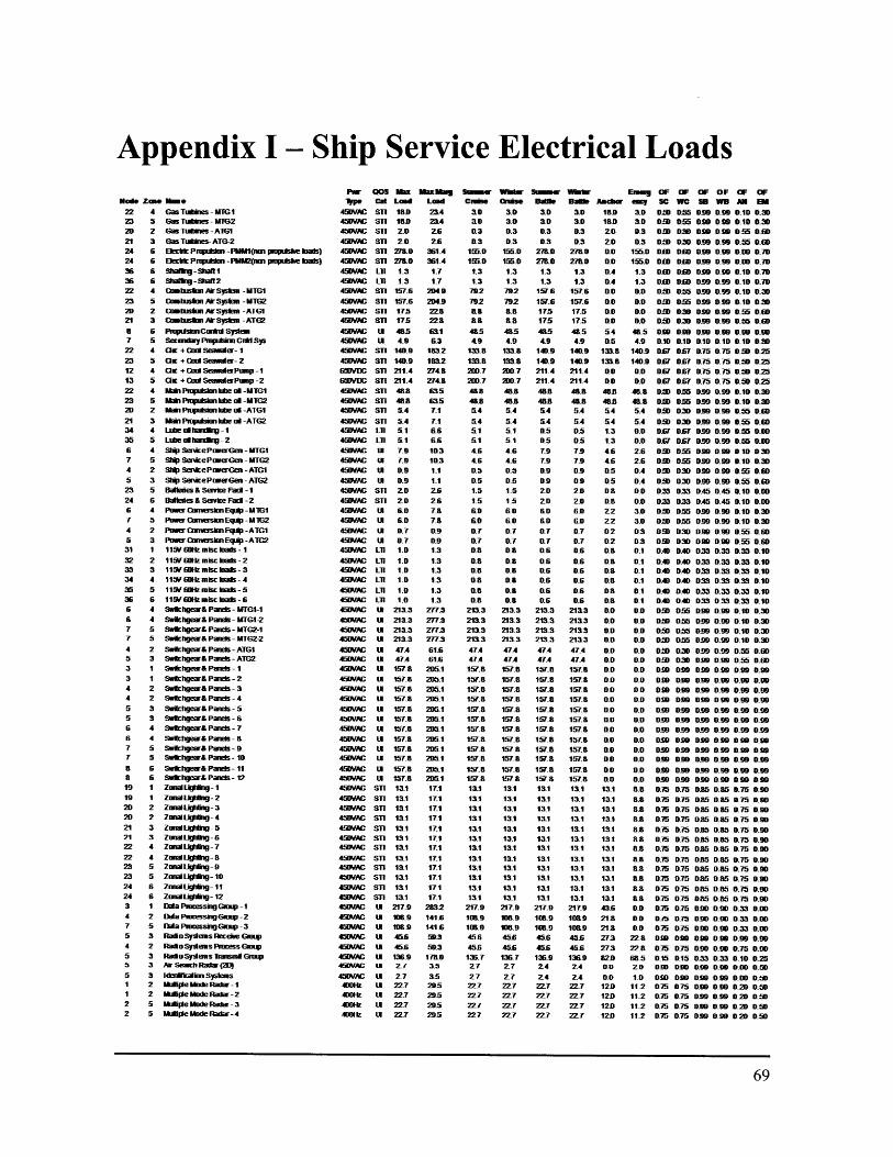
N
0
"-N
wW
WN
W
-M
O. -
N
MM
MM
W
N
-' ii
iii
&
i f
Ns -
WN.
oils
ER
11[11M
pl~~itr31
p+ +
; r g~i
-o
saw
~ R~
R~ n
I~
t I% Hi
Ril.
i-4
M
9,9
A
,0
8
KI BC
in
o 1050
~IVI
WN
'1IZ
rr r
HO
cn
uwh~
- ,-$i
B
HI ýr Ct
CA
CD
9 r 0
Ng;
;g
ggg;
ii
N '
iiN
N4
4 04
0 a
oC)C
a RI.......
(O--
---
wuw
uC~
b'sb
bb
*i~~
99ru
N
8~
9 7
-
NN
4
pt.
ýU
lm
Qu
ip
WO
W W
-4
p""
-------------
w w
v.
NU
U14
pp p
op
Opp
M
mý,
-p
pf~
k ppp
A&
-
p $
$ P
00)
C
MwM-4
-4 000iwu
vmm-bP
0t
00W
0
cc
iiriW00iM
ii,,,
i-i
i tii
to~
~w
ww
uWuw
i0
0U
U0
0W
hb~
iDjji
~p
~L~(
WO
Og
8wY
..
~~~~,,,
, UcUoUc
Oc
coc
soo
Co
ocM
IM
OOOOC4C-N
ag
t
0 via
POOinaMOO
--
wo
I 0w
w
w
c A
A
;-4
--4
-&
-
Go
0 A
b dNoa
0a
0
L
~b cc
a
.....
.cc
coo c
oo
c o
coo COCOON N
w
ONNNNMPOOMM w
w a-
& bo
be c
PPPO
OPP
PPPP
P9
p999
99
PPPp
PPP
a aa
@m
~sa
ssss
s
005
9P
P
PP8
als
p0P
0000
0000
8383
00000000000
P999
9PPP
PPa8
8888
8888
8PP
PPPP
PP
gsas3
asg
g.g
00000500000.o
31
31
33
33
33
31
3
lli 199
3888 q999 ssee
gig
0il
050
tat
000
888 "pp Iss
PPq
3S3
000000000050
pp
pp
pp
pp
pp
~p
O
fl85aus 38831
coo
pppo
pppo
ppp
ppoo
oooo
oooa
ooss
assa
us
00055000
obiu
illi
basso
ossPP
PPPP
PPta
maaa~
a00000555
1311
33
sis
pp
pp
pp
pp
881S
8888
aaa gig
tat
13fl
"pp 16
66Co
oso
$
so@
0000500
oot3
at
0000500
$ui3
liin
illi3
PP
00P
P05
am
a
33Se
0000
000
8113
sea6
818
PPPP
PP0
tUn
ue 88
.oo
ooo
.oio
I I p a
111.
omM
1111
1 EM
5~
EM~
Z~
~Z
~E
PM
Mg
~b
b~
b~
~b
oo
ob
~b
bb
bb
bb
89
9X
Xg
g~
bb
orpP
ooPp
pp~a
oooo
ooo
oooo
oooo
o w
woo
~O
P
r~bb
b~io
~bbg
bbbo
bbbb
~

ll8888!!3
!3emcee cecce
8885555(e
mce
e ccc
ee
M9
88
2
33
dddddddd
ddddcdddd
RRRRRRRAd
dd
dd
dd
!B2222RR2
oooaaems
258528
dlddilli
imeecc e
solese
ce
ae
22222
ceeceo
2*2
*8
88888
88888
emcee
l l
21112moo
ccmCCOcES
cc eeeem
emd
58888
8
2;dddddodd
dd!$B
llin955
~88588885852;
cc eacecceem
eq
illill
9dc
oW8 28
aes
min
d
i .
R"2
d d r
3sess3es
ddedddd
dddd9d
c99d5
ccc
ccc
macac
3s3
98
8cde
888
ccc
HE
38dd
eec
888
8aseed
888
db
d
ddddcdc
AmA222
3838883f888l N
33E
8888
eededdcdddcdddddddcdd
93
99
98
83
33
33
93
s3
93
83
sdcddddddddcdddddedddd
5~
~~
88588855885888W
lddileeccelcceec
ccc
illlll588888855855888
aecceeccecee
acel
eemj
Ro
ecceceec
dddccd
ld
dd dd
id R4 0o
0
p- 4t qt
qt qt It
it lql
urý q!
m
r.- Pý
0 am
a a a 0
9090 O
3 3 5 SEE ~
~
W
8~~~~
ww
ww
P00qd'"S
ijj ;;;6b6B
b ;; ·
i r!-~
5S
S
e
3d~
8i2
2
iacecaw
i;;;e
m8
i
2a
99
e
nu
co
s
ccscs
hg
---
~
m
ee
eq
m
fleemP
cc apeinehco
jt N
ooa -w
m
n
aasol e
c
c c
P m
-------------eccace
ecceecc~c~so
*Na--
-flfle0cww
99P0c
3 qN
N
NNc
N
""" ·
~ ceNcccieaSmnna
5
~5 55555~
~55~
~5555555555 s55,5
5~
~
R"" R R R
RH 01111 M
RUH RR-ý Rlýý UN RH -ýRR RRR 1R
ý ýR-ý -ý*
BQ
9bQ
~b
Nflt.~
NI
nhfi IIBFB
%%
I I!!ivIiiiiP
I"1111111111
111~ F8 rr.
-
I88iHHHH8ui mn!!!!!I ja
nq'nw
IT
II?
ul tI U
9 69.
,7 ? -N m
-ý ?I
Q
VU
W
1
Ij 1¾.NflU
Nf
1r. 1 ~br
.i g &
g -, -
-i .7
i1iýilar r
&
7 11N
183 A
in 3g
111
1 7 jIIII'itiii
-oo
l NL
Ir Iralll'
88888
s 8eeB
e
mcee
lee
vd d 6
coo
cc
3s3
dd
da
i d
d8118
cco
ee
oa
~~~~~AR
~AA
~B18~W
W~B
~~~W~~~~~~~a~=
P~~~f~~
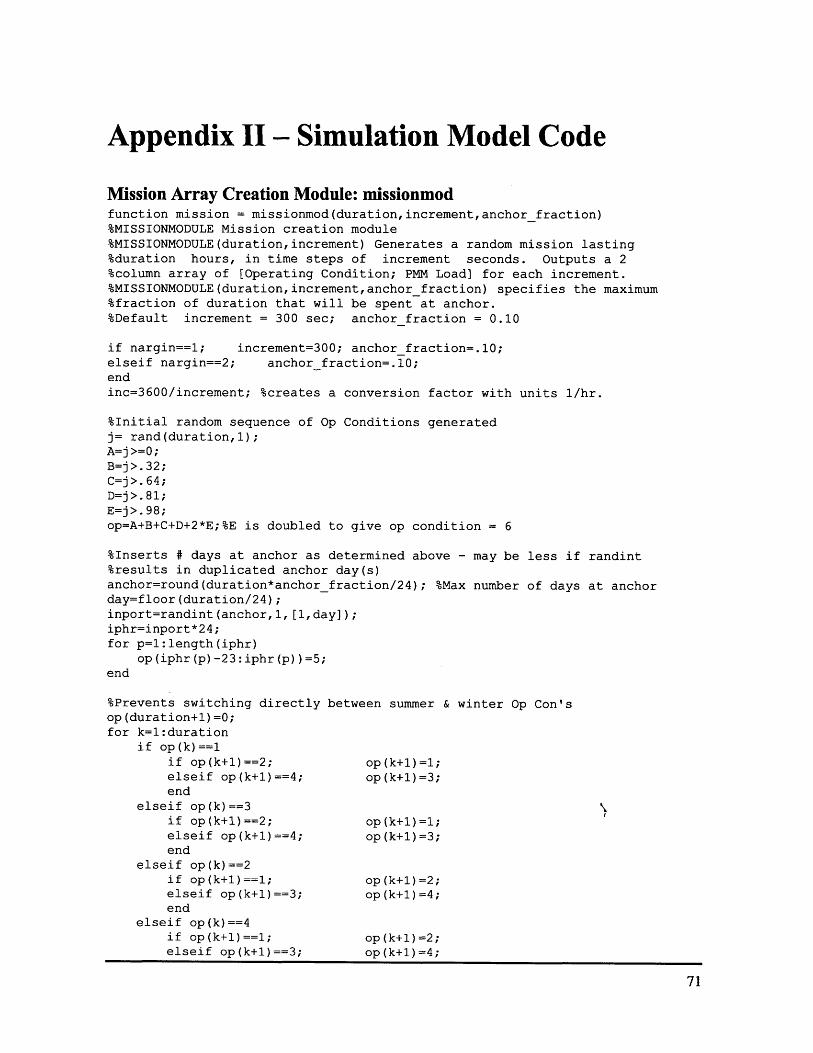
Appendix II- Simulation Model Code
Mission Array Creation Module: missionmodfunction mission = missionmod(duration,increment,anchorfraction)%MISSIONMODULE Mission creation module%MISSIONMODULE(duration,increment) Generates a random mission lasting%duration hours, in time steps of increment seconds. Outputs a 2%column array of [Operating Condition; PMM Load] for each increment.%MISSIONMODULE(duration,increment,anchor fraction) specifies the maximum%fraction of duration that will be spent at anchor.%Default increment = 300 sec; anchor fraction = 0.10
if nargin==l; increment=300; anchor fraction=.10;elseif nargin==2; anchor fraction=.10;endinc=3600/increment; %creates a conversion factor with units 1/hr.
%Initial random sequence of Op Conditions generatedj= rand(duration, );A=j>=0;B=j>.32;C=j>.64;D=j>.81;E=j>.98;op=A+B+C+D+2*E;%E is doubled to give op condition = 6
%Inserts # days at anchor as determined above - may be less if randint%results in duplicated anchor day(s)anchor=round(duration*anchor_fraction/24); %Max number of days at anchorday=floor(duration/24);inport=randint(anchor, ,[, day]);iphr=inport*24;for p=l :length(iphr)
op(iphr(p)-23:iphr(p)) =5;end
%Prevents switching directly between summer & winter Op Con'sop(duration+l)=0;for k=l:duration
if op(k)==1if op(k+l)==2; op(k+l)=1;elseif op(k+l)==4; op(k+l)=3;end
elseif op(k)==3 \if op(k+l)==2; op(k+l)=l;elseif op(k+l)==4; op(k+l)=3;end
elseif op(k)==2if op(k+l)==1; op(k+l)=2;elseif op(k+l)==3; op(k+l)=4;end
elseif op(k)==4if op(k+l)==1; op(k+l)=2;elseif op(k+l)==3; op(k+l)=4;

endend
endop=op (:duration);
%Expands op from hours to chosen increment, now called "opcon"op=op';opcon=op(ones(l,inc),:);%replaces function: opcon=repmat(op,inc,1);opcon=opcon (:);
%Randomly generates propulsion loads at each incrementy=rand(length(opcon),1);F=opcon<3; %cruise conditionsG=(opcon>2 & opcon <5); %battle conditionsH=opcon>5; %emergency conditionI=(F==l & y>=.05 & y<.25); I=I*1730;J=(F==l & y>=.25 & y<.45); J=J*1903;K=(F==l & y>=.45 & y<.55); K=K*2595;L=(F==1 & y>=.55 & y<.65); L=L*2855;M=(F==1 & y>=.65 & y<.775); M=M*6055;N=(F==1 & y>=.775 & y<.9); N=N*6667;P=(F==1 & y>=.9 & y<.95); P=P*13840;Q=(F==1 & y>=.95); Q=Q*13096;R=(G==1 & y>=.05 & y<.3); R=R*1730;S=(G==1 & y>=.3 & y<.7); S=S*6055;T=(G==1 & y>=.7 & y<.85); T=T*13840;U=(G==1 & y>=.85); U=U*67773;V=(H==1 & y>=.35 & y<.5); V=V*1730;W=(H==l & y>=.5 & y<.65); W=W*1903;X=(H==1 & y>=.65 & y<.725); X=X*2595;Y=(H==1 & y>=.725 & y<.8); Y=Y*2855;Z=(H==1 & y>=.8 & y<.825); Z=Z*6055;AA=(H==l & y>=.825 & y<.85); AA=AA*6667;BB=(H==1 & y>=.85 & y<.925); BB=BB*13840;CC=(H==l & y>=. 92 5); CC=CC*13096;%sum above to get pmm load vectorpmm = I+J+K+L+M+N+P+Q+R+S+T+U+V+W+X+Y+Z+AA+BB+CC;
%output operating condition and pmm load at each incrementmission=[opcon pmm];
Power Load Array Creation Module: loadmodfunction loadnode = loadmod(mission,PLMt)%LOADMOD Load generator module%LOADMOD(mission) takes the inputs from mission [opcon pmm] and outputs the%load required at each load node for each increment as the%(increments x nodes) array loadnode containing the node and required load%for each increment.
opcon = mission(:,l);pmm=mission(:,2);inc=length(opcon);A=rand(inc,193);%random array to compare with OFs to see if loads on or off%Run loop to get individual loads by increment
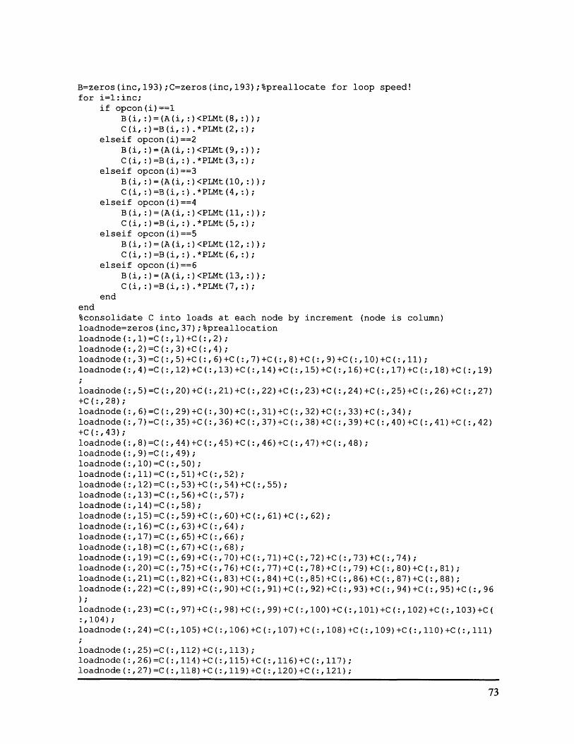
B=zeros(inc,193);C=zeros(inc,193);%preallocate for loop speed!for i=l:inc;
if opcon(i)==1B(i,:)=(A(i,:)<PLMt(8,:));C(i, :)=B(i, :) .*PLMt (2,:);
elseif opcon(i)==2B(i,:)=(A(i,:)<PLMt(9,:));C(i, :)=B(i, :) .*PLMt(3,:);
elseif opcon(i)==3B(i,:)=(A(i,:)<PLMt(10,:));C(i,:)=B(i,:).*PLMt(4,:);
elseif opcon(i)==4B(i,:)=(A(i,:)<PLMt(11,:));C(i,:)=B(i,:).*PLMt(5,:);
elseif opcon(i)==5B(i,:)=(A(i,:)<PLMt(12,:));C(i, :)=B(i, :) .*PLMt(6,:);
elseif opcon(i)==6B(i,:)=(A(i, : ) <PLMt(13,:));C(i, :)=B(i, :).*PLMt (7,:)
endend%consolidate C into loads at each node by increment (node is column)loadnode=zeros(inc,37);%preallocationloadnode(:,1)=C(:,1)+C(:,2);loadnode(:,2)=C(:,3)+C(:,4);loadnode(:,3)=C(:,5)+C(:,6)+C(:,7)+C(:,8)+C(:,9)+C(:,10)+C(:,11);loadnode(:,4)=C(:,12)+C(:,13)+C(:,14)+C(:,15)+C(:,16)+C(:,17)+C(:,18)+C(:,19)
loadnode(:,5)=C(:,20)+C (:,21)+C(:,22)+C(:,23)+C(:,24)+C(:,25)+C(:,26)+C(:,27)+C(:,28);loadnode(:,6)=C(:,29)+C(:,30)+C(:,31)+C(:,32)+C(:,33)+C(:,34);loadnode(:,7)=C(:,35)+C(:,36)+C(:,37) +C(:,38)+C(:,39)+C(:,40)+C(:,41)+C(:,42)+C(:,43);loadnode(:,8)=C(:,44)+C(:,45)+C(:,46)+C(:,47)+C(:,48);loadnode(:, 9)=C(:,49);loadnode ( :,10) =C (:, 50);loadnode(:,11)=C(:,51)+C(:,52);loadnode(:,12)=C(:,53)+C(:,54)+C(:,55);loadnode(:,13)=C(:,56)+C(:,57);loadnode(:,14)=C(:,58);loadnode(:,15)=C(:,59)+C(:,60)+C(:,61)+C(:,62);loadnode(:,16)=C(:,63)+C(:,64);loadnode(:,17)=C(:,65)+C(:,66);loadnode(:,18)=C(:,67)+C(:,68);loadnode(:,19)=C(:,69)+C(:,70)+C(:,71)+C(:,72)+C(:,73)+C(:,74);loadnode(:,20)=C(:,75)+C(:,76) +C(:,77) +C(:,78)+C (:,79)+C (:,80)+C (:,81);loadnode(:,21)=C(:,82)+C(:,83)+C(:,84)+C(:,85)+C(:,86)+C(:,87)+C(:,88);loadnode(:,22)=C(:,89)+C(:,90)+C(:,91)+C(:,92)+C(:,93)+C(:,94)+C(:,95)+C(:,96
loadnode(:,23)=C(:,97)+C(:,98)+C(:,99)+C(:,100)+C(:,101)+C(:,102)+C(:,103)+C(:,104);loadnode(:,24)=C(:,105)+C(:,106)+C(:,107)+C(:,108)+C(:,109)+C(:,110)+C(:,111)
loadnode(:,25)=C(:,112)+C(:,113);loadnode(:,26)=C(:,114)+C(:,115)+C(:,116)+C(:,117);loadnode(:,27)=C(:,118)+C(:,119)+C(:,120)+C(:,121);

loadnode(:,28)=C(:,122)+C(:,123)+C(:,124);loadnode(:,29)=C(:,125)+C(:,126)+C(:,127);loadnode(:,30)=C(:,128)+C(:,129);loadnode(:,31)=C(:,130)+C(:,131)+C(:,132)+C(:,133)+C(:,134)+C(:,135)+C(:,136)+C(:,137)+C(:,138)+C(:,139)+C(:,140);loadnode(:,32)=C(:,141)+C(:,142)+C(:,143)+C(:,144)+C(:,145)+C(:,146)+C(:,147)+C(:,148)+C(:,149)+C(:,150)+C(:,151)+C(:,152)+C(:,153)+C(:,154);loadnode(:,33)=C(:,155)+C(:,156)+C(:,157)+C(:,158)+C(:,159)+C(:,160)+C(:,161)+C (:,162) +C (:,163);loadnode(:,34)=C(:,164)+C(:,165)+C(:,166)+C(:,167)+C(:,168)+C(:,169)+C(:,170)
loadnode(:,35)=C(:,171)+C(:,172)+C(:,173)+C(:,174)+C(:,175)+C(:,176)+C(:,177)+C (:,178) +C (:,179);loadnode (:,36)=C(:,180)+C(:,181)+C(:,182)+C(:,183)+C(:,184)+C(:,185)+C ( :, 186)+C(:,187)+C(:,188) +C((:,1190)+C(:,191)+C(:,192)+C(:,193);loadnode (:,37)=pmm;
Power Generation Capacity Array Creation Module: pgmmodfunction pwrgen = pgmmod(mission,MTBF)%PGMMOD Power generation simulation module%PGMMOD(mission) takes the inputs from mission [opcon pmm] and%available power produced by the pgm for each increment as the
outputs thecolumn
%vector pwrgen. Module includes PGM availability based on ship operating%condition, PGM faults, repairs, and standby PGM.
opcon = mission(:,l);inc=length(opcon);%Set PGM Reliability and Maintenance meansmtbf=MTBF(1)*12*ones(10,4);%Default MTBF per PGM is 1000 hrs, 5 minincrementsmttr=5*12*ones(10,4);%Default MTTR per PGM is 5 hrs
%Set engines ON array pgm: 1 MTG for Cruise, 2 MTG for Battle, 2 ATG for%Anchor, 1 ATG for Emergencypgm=zeros(inc,4); %preallocate 4 columns for engines [MTG MTG ATG ATG]for i=l:inc;
if opcon(i)==1 11 opcon(i)== 2pgm(i,1)= (1);
elseif opcon(i)==3 II opcon(i)== 4pgm(i,1:2)= (1);
elseif opcon(i)== 5pgm(i,3:4)= (1);
elseif opcon(i)== 6pgm(i,3)= (1);
endend
%Create Random Engine Failures & Repairs (exponential distribution)lambda=l./mtbf;mu=l./mttr;u=rand(10,4);TF=ceil(-log(u)./lambda);u=rand(10,4);TR=ceil(-log(u)./mu);TA=TR;
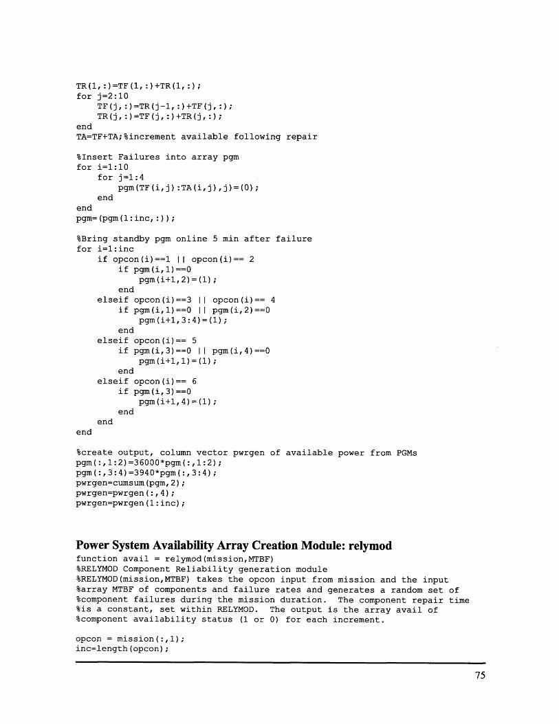
TR(, :)=TF(1,:)+TR(1,:);for j=2:10
TF(j,:)=TR(j-1,:)+TF(j,:);TR(j, :)=TF(j, :)+TR(j,:) ;
endTA=TF+TA;%increment available following repair
%Insert Failures into array pgmfor i=1:10
for j=1:4pgm(TF(i,j):TA(i,j),j)=(O);
endendpgm=(pgm(l:inc,:));
%Bring standby pgm online 5 min after failurefor i=1l:inc
if opcon(i)==l I opcon(i)== 2if pgm(i,l)==0
pgm(i+1, 2) =(1);end
elseif opcon(i)==3 II opcon(i)== 4if pgm(i,l)==0 I pgm(i,2)==0
pgm(i+1,3:4)=(1);end
elseif opcon(i)== 5if pgm(i,3)==0 II pgm(i,4)==0
pgm(i+l,l)=(l);end
elseif opcon(i)== 6if pgm(i,3)==0
pgm(i+1,4)=(1);end
endend
%create output, column vector pwrgen of available power from PGMspgm(:,1:2)=36000*pgm(:,1:2);pgm(:,3:4)=3940*pgm(:,3:4);pwrgen=cumsum(pgm,2);pwrgen=pwrgen(:,4);pwrgen=pwrgen (:inc);
Power System Availability Array Creation Module: relymodfunction avail = relymod(mission,MTBF)%RELYMOD Component Reliability generation module%RELYMOD(mission,MTBF) takes the opcon input from mission and the input%array MTBF of components and failure rates and generates a random set of%component failures during the mission duration. The component repair time%is a constant, set within RELYMOD. The output is the array avail of%component availability status (1 or 0) for each increment.
opcon = mission(:,l);inc=length(opcon);

MTBF=MTBF(2:172);RT=5;%number of increments to repair component (total downtime is RT+1)
%Generate random time to failure for each component using exponential distlambda=1./(MTBF*12);%12 expands to 5 min incrementsu=rand(length(MTBF),1);TF=ceil(-log(u)./lambda);TF=min(TF,inc+l);%makes inc+l1 the upper bound for TF, will cut off later
%Insert failures intoavail=ones(inc+l,171);avail(TF(1),1)=0;avail(TF(2),2)=0;avail (TF(3), 3)=0;for i=4:171
avail(TF(i) :TF(i)+RT,i)=0;endavail(inc+l :inc+l+RT,:)=[];
Power System Operational Evaluation Module: pwrsysmodfunction pwrnode = pwrsysmod(avail)%PWRSYSMOD Power System Evaluation Module%PWRSYSMOD(avail) evaluates the power system%for the supplied component availability, and outputs the array pwrnode%containing the available power at each node for each increment.
opcon = avail(:,l);inc=length(opcon);pwrnode=zeros(inc,37);%for output column 37 is for total bus power below
%but will be changed to pmm pwr available in qosmod
%PCM-4 failures accounted for and impact on Port/Stbd bussesport=ones(inc, );stbd=ones(inc, );for i=l:inc
if avail(i,l)==l && avail(i,2)==l && avail(i,3)==lelseif avail(i,1)==0 11 avail(i,3)==0port(i)=0;elseif avail(i,2)==0stbd(i)=0;end
endpwrnode(:,37)=6880*(port+stbd);%6880KW capacity per PCM-4, 1 PCM-4 per buscap=300*avail;%300KW capacity per SSCM/SSIM
%Zone 1%available sscm capacity per incrementsscm650p_1=port.*sum(cap(:,4),2);%can remove sum if only 1 columnsscm650s l1=stbd.*sum(cap(:,9),2);sscm800p_l=port.*sum(cap(:,5:8),2);sscm800s 1=stbd.*sum(cap(:,10:13),2);%available ssim capacity per incrementssim400 1=sum(cap(:,14:15),2);ssim60 1=min(sum(cap(:,16:21),2),sscm800p_l+sscm800s 1-ssim400 1);
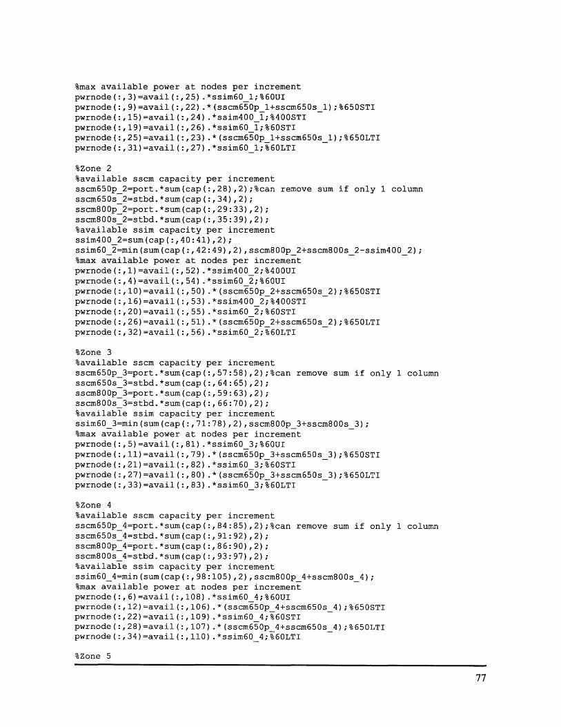
%max available power at nodes per incrementpwrnode(:,3)=avail(:,25).*ssim60_1;%60UIpwrnode(:,9)=avail(:,22).*(sscm650p_l+sscm650s_1);%650STIpwrnode(:,15)=avail(:,24).*ssim400_ ;%400STIpwrnode(:,19)=avail(:,26).*ssim60 _1;%60STIpwrnode(:,25)=avail(:,23) .*(sscm650p_l+sscm650s 1) ;%650LTIpwrnode(:,31)=avail(:,27).*ssim60O1;%60LTI
%Zone 2%available sscm capacity per incrementsscm650p_2=port.*sum(cap(:,28),2);%can remove sum if only 1 columnsscm650s 2=stbd.*sum(cap(:,34),2);sscm800p 2=port.*sum(cap(:,29:33),2);sscm800s 2=stbd.*sum(cap(:,35:39),2);%available ssim capacity per incrementssim400 2=sum(cap(:,40:41),2);ssim60_2=min(sum(cap(:,42:49),2),sscm800p 2+sscm800s_2-ssim400_2);%max available power at nodes per incrementpwrnode(:,1)=avail(:,52).*ssim400_2;%400UIpwrnode(:,4)=avail(:,54).*ssim60 2;%60UIpwrnode(:,10)=avail(:,50).*(sscm650p 2+sscm650s 2);%650STIpwrnode(:,16)=avail(:,53).*ssim400 2;%400STIpwrnode(:,20)=avail(:,55).*ssim60 2;%60STIpwrnode(:,26)=avail(:,51).*(sscm650p 2+sscm650s 2);%650LTIpwrnode(:,32)=avail(:,56).*ssim60 2;%60LTI
%Zone 3%available sscm capacity per incrementsscm650p_3=port.*sum(cap(:,57:58),2);%can remove sum if only 1 columnsscm650s_3=stbd.*sum(cap(:,64:65),2);sscm800p 3=port.*sum(cap(:,59:63),2);sscm800s 3=stbd.*sum(cap(:,66:70),2);%available ssim capacity per incrementssim60_3=min(sum(cap(:,71:78),2),ssm800p3+sscm800s 3);%max available power at nodes per incrementpwrnode(:,5)=avail(:,81).*ssim60 3;%60UIpwrnode(:,11)=avail(:,79).*(sscm650p_3+sscm650s_3);%650STIpwrnode(:,21)=avail(:,82).*ssim60 3;%60STIpwrnode(:,27)=avail(:,80).*(sscm650p_3+sscm650s 3);%650LTIpwrnode(:,33)=avail(:,83).*ssim60 3;%60LTI
%Zone 4%available sscm capacity per incrementsscm650p_4=port.*sum(cap(:,84:85),2);%can remove sum if only 1 columnsscm650s 4=stbd.*sum(cap(:,91:92),2);sscm800p_4=port.*sum(cap(:,86:90),2);sscm800s_4=stbd.*sum(cap(:,93:97),2);%available ssim capacity per incrementssim60 4=min(sum(cap(:,98:105),2),sscm800p 4+sscm800s_4);%max available power at nodes per incrementpwrnode(:,6)=avail(:,108).*ssim60 4;%60UIpwrnode(:,12)=avail(:,106).*(sscm650p_4+sscm650s_4);%650STIpwrnode(:,22)=avail(:,109).*ssim60 4;%60STIpwrnode(:,28)=avail(:,107).*(sscm650p 4+sscm650s 4);%650LTIpwrnode(:,34)=avail(:,110).*ssim60 4;%60LTI
%Zone 5

%available sscm capacity per incrementsscm650p 5=port.*sum(cap(:,ll1:112),2);%can remove sum if only 1 columnsscm650s 5=stbd.*sum(cap(:,119:120),2);sscm800p 5=port.*sum(cap(:,113:118),2);sscm800s 5=stbd.*sum(cap(:,121:126),2);%available ssim capacity per incrementssim400 5=sum(cap(:,127:128),2);ssim60 5=min(sum(cap(:,129:136),2),sscm800p 5+sscm800s 5-ssim400 5);%max available power at nodes per incrementpwrnode(:,2)=avail(:,139).*ssim400 5;%400UIpwrnode(:,7)=avail(:,141).*ssim60 5;%60UIpwrnode(:,13)=avail(:,137).*(sscm650p 5+sscm650s 5);%650STIpwrnode(:,17)=avail(:,140).*ssim400 5;%400STIpwrnode(:,23)=avail(:,142).*ssim60 5;%60STIpwrnode(:,29)=avail(:,138).*(sscm650p 5+sscm650s_5);%650LTIpwrnode(:,35)=avail(:,143).*ssim60 5;%60LTI
%Zone 6%available sscm capacity per incrementsscm650p_6=port.*sum(cap(:,144),2);%can remove sum if only 1 columnsscm650s 6=stbd.*sum(cap(:,150),2);sscm800p 6=port.*sum(cap(:,145:149),2);sscm800s 6=stbd.*sum(cap(:,151:155),2);%available ssim capacity per incrementssim400 6=sum(cap(:,156:157),2);ssim60 6=min(sum(cap(:,158:165),2),sscm800p 6+sscm800s 6-ssim400 6);%max available power at nodes per incrementpwrnode(:,8)=avail(:,169).*ssim60 6;%60UIpwrnode(:,14)=avail(:,166).*(sscm650p 6+sscm650s 6);%650STIpwrnode(:,18)=avail(:,168).*ssim400 6;%400STIpwrnode(:,24)=avail(:,170).*ssim60 6;%60STIpwrnode(:,30)=avail(:,167).*(sscm650p 6+sscm650s 6);%650LTIpwrnode(:,36)=avail(:,171).*ssim60 6;%60LTI
Quality of Service Failure Evaluation Module: qosmodfunction QOS = qosmod(loadnode,pwrnode,pwrgen)%QOSMOD Quality of Service Evaluation module%QOSMOD(loadnode,pwrnode) Compares the input arrays and determines (1)if a%QOS failure has occurred, (2)when it occurred, and (3)at which node.%Outputs an array of nodes and increments that experience a QOS failure.
inc=length(pwrgen);%bustotal=pwrnode(:,37);%total pwr from port & stbd bussesssreq=sum(loadnode(:,1:36),2);%total pwr req for ship service usepwrnode(:,37)=pwrgen-ssreq;%pwr available for pmm use%busfail=max(ssreq-bustotal,0);%amount to shed due to bus loss (PCM-4 fail)loadnode(:,37)=min(loadnode(:,37),43880);%cut off qos "exempt" pmm load
A=loadnode > pwrnode;%B=A(2:inc,25:37);B(inc,l:13)=zeros(l,13);A(:,25:37)=(A(:,25:37) & B);[I,JJ=find(A);
QOS=[I J];

Master Simulation Module: Monte XX%Monte XX%Performs the Monte Carlo Simulation and gathers relevant statistical data%for the MCS for experiment number XX. **Must change input MAT-file%MTBF XX below and also SAVE filename Monte XX at bottom for each trial XX.%Note:uses function randint.m from Communications Toolbox
clear all; clcload PLMt;load MTBF XX;runs=1000;%# of simulation runs
%loop to conduct desired number of runs through IPS sim modelincfail=zeros(500,runs);%preallocatenodefail=zeros(500,runs);numfail=zeros (, runs);firstfail=zeros(l,runs);pmnumfail=zeros (, runs);pmfirstfail=zeros (, runs);for i=l:runs
mission = missionmod(4380);
pwrgen=pgmmod(mission,MTBF);
loadnode=loadmod(mission,PLMt);
avail = relymod(mission,MTBF);
pwrnode = pwrsysmod(avail);
QOS=qosmod(loadnode,pwrnode,pwrgen);
incfail(l:length(QOS),i)=QOS(:,l);%increments of failure for runnodefail(l:length(QOS),i)=QOS(:,2);%nodes of failure for runnumfail(i)=length(QOS);%number of failures for runfirstfail(i)=min(QOS(:,l));%increment of first failure for run%now exclude pmm failurespmcanx=(QOS(:,2) =37);pmqos=QOS(:, ).*pmcanx;pmqos(pmqos==0)=[];pmnumfail(i)=length(pmqos);if -isempty(pmqos)
pmfirstfail(i)=(min(pmqos));else
pmfirstfail(i)=length(pwrgen);end
end
%compile data for all QOS failuresifail=incfail(:);ifail(ifail==0)=[];nfail=nodefail(:);nfail(nfail==0)=[];fail(:,l)=ifail(:);fail(:,2)=nfail(:) ;%compile data excluding pmm QOS failures

pmcanx= (nfail-~=37);ifail=ifail.*pmcanx;ifail(ifail==0)=[];nfail=nfail.*pmcanx;nfail(nfail==0)=[];pmfail(:,) =ifail(:);pmfail(:,2)=nfail(:);
%Calculate and save relevant statistical data%mean first failureFirstFail=mean(firstfail);%mean first failure excluding PMM failuresFirstFail noPMM=mean(pmfirstfail);%mean # failuresNumFail=mean(numfail);%mean # failures excluding PMM failuresNumFail noPMM=mean(pmnumfail);%percent of failures at each noden=histc(fail(:,2),1:37);NodePct=100*n/length(fail);NodeMaxModePct=[find(n==max(n)) max(n) max(NodePct)];%percent of failures at each node excluding PMM failuresnpm=histc(pmfail(:,2),1:36);NodePct noPMM=100*npm/length (pmfail);NodeMaxModePct noPMM=[find(npm==max(npm)) max(npm) max(NodePct noPMM)];
%Save a MAT-file of the simulation statistical results (* includes noPMM)save('DataXX', 'FirstFail*', 'NumFail*', 'n', 'npm', 'Node*', 'fail','pmfail');
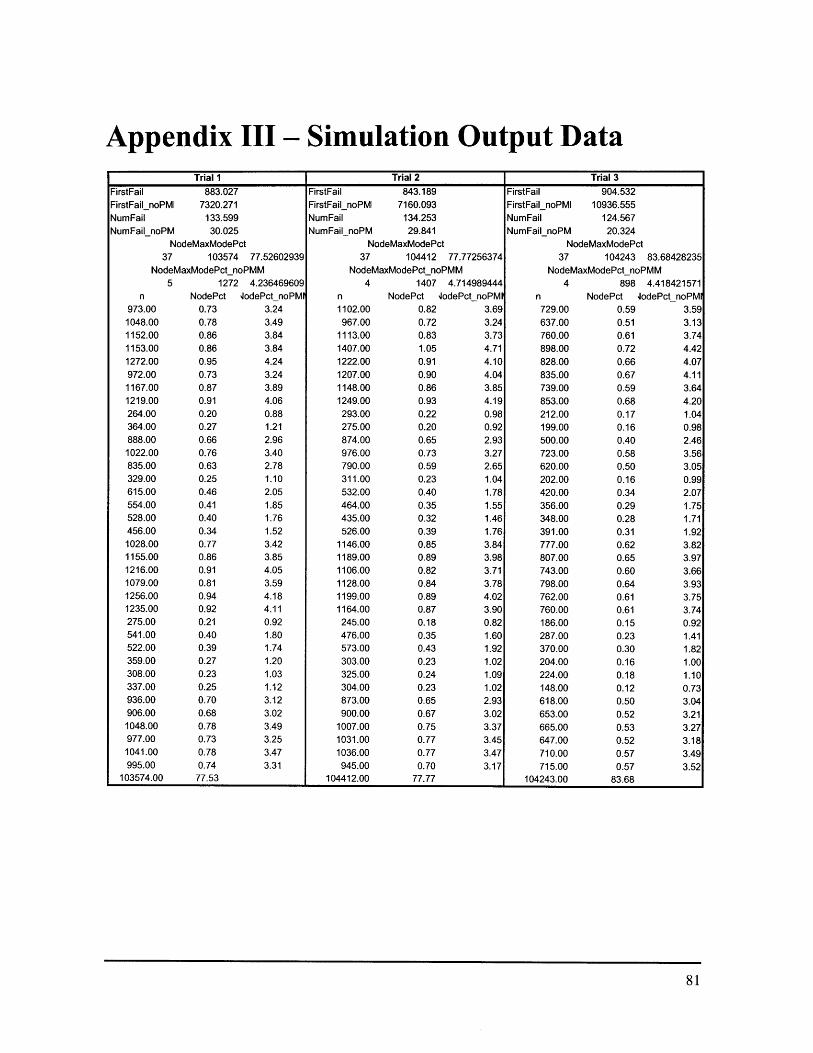
Appendix III - Simulation Output DataTrial 1
FirstFail 883.027FirstFail noPMI 7320.271NumFail 133.599NumFail noPM 30.025
NodeMaxModePct37 103574 77.52602939
NodeMaxModePctnoPMM
n973.001048.001152.001153.001272.00972.001167.001219.00264.00364.00888.001022.00835.00329.00615.00554.00528.00456.001028.001155.001216.001079.001256.001235.00275.00541.00522.00359.00308.00337.00936.00906.00
1048.00977.00
1041.00995.00
103574.00
1272NodePct
0.730.780.860.860.950.730.870.910.200.270.660.760.630.250.460.410.400.340.770.860.910.810.940.920.210.400.390.270.230.250.700.680.780.730.780.7477.53
4.2364696094odePct noPMI
3.243.493.843.844.243.243.894.060.881.212.963.402.781.102.051.851.761.523.423.854.053.594.184.110.921.801.741.201.031.123.123.023.493.253.473.31
Trial 2FirstFail 843.189FirstFail noPMI 7160.093NumFail 134.253NumFail noPM 29.841
NodeMaxModePct37 104412 77.77256374
NodeMaxModePct noPMM4
n1102.00
967.001113.001407.001222.001207.001148.001249.00293.00275.00874.00976.00790.00311.00532.00464.00435.00526.00
1146.001189.001106.001128.001199.001164.00245.00476.00573.00303.00325.00304.00873.00900.00
1007.001031.001036.00945.00
104412.00
1407 4.714989444NodePct 4odePct noPMI
0.820.720.831.050.910.900.860.930.220.200.650.730.590.230.400.350.320.390.850.890.820.840.890.870.180.350.430.230.240.230.650.670.750.770.770.70
77.77
Trial 3FirstFail 904.532FirstFail noPMI 10936.555NumFail 124.567NumFail noPM 20.324
NodeMaxModePct37 104243 83.68428235
NodeMaxModePct noPMM
n729.00637.00760.00898.00828.00835.00739.00853.00212.00199.00500.00723.00620.00202.00420.00356.00348.00391.00777.00807.00743.00798.00762.00760.00186.00287.00370.00204.00224.00148.00618.00653.00665.00647.00710.00715.00
104243.00
898 4.418421571NodePct 4odePct noPMI
0.59 3.590.51 3.130.61 3.740.72 4.420.66 4.070.67 4.110.59 3.640.68 4.200.17 1.040.16 0.980.40 2.460.58 3.560.50 3.050.16 0.990.34 2.070.29 1.750.28 1.710.31 1.920.62 3.820.65 3.970.60 3.660.64 3.930.61 3.750.61 3.740.15 0.920.23 1.410.30 1.820.16 1.000.18 1.100.12 0.730.50 3.040.52 3.210.53 3.270.52 3.180.57 3.490.57 3.52
83.68
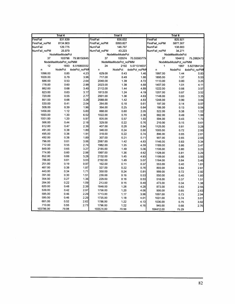
Trial 4FirstFail 831.639FirstFail noPMI 8134.903NumFail 129.775NumFail noPM 25.979
NodeMaxModePct37 103796 79.98150645
NodeMaxModePctnoPMM12 1693 6.516802032
n NodePct IodePctnoPMI1098.001028.00686.00778.00882.00823.00720.00851.00530.00508.00
1456.001693.001551.00
566.00612.00491.00495.00492.00796.00712.00849.00774.00852.00786.00251.00487.00443.00391.00354.00284.00620.00539.00595.00595.00681.00710.00
103796.00
0.850.790.530.600.680.630.550.660.410.391.121.301.200.440.470.380.380.380.610.550.650.600.660.610.190.380.340.300.270.220.480.420.460.460.520.55
79.98
4.233.962.642.993.403.172.773.282.041.965.606.525.972.182.361.891.911.893.062.743.272.983.283.030.971.871.711.511.361.092.392.072.292.292.622.73
Trial 5FirstFail 836.032FirstFail noPMI 5093.827NumFail 146.797NumFail noPM 43.223
NodeMaxModePct37 103574 70.55593779
NodeMaxModePctnoPMM24 2192 5.071374037
n629.00717.00
2040.002023.002112.001813.002001.002088.00
264.00364.00888.00
1022.00835.00329.00407.00346.00318.00307.00
2087.001982.002185.001997.002132.002192.00
162.00327.00350.00230.00229.00213.00
1848.001756.001713.001735.001786.001796.00
103574.00
1.461.664.724.684.894.194.634.830.610.842.052.361.930.760.940.800.740.714.834.595.064.624.935.070.370.760.810.530.530.494.284.063.964.014.134.16
Trial 6FirstFail 825.921FirstFail noPMI 5977.307NumFail 138.683NumFailnoPM 34.271
NodeMaxModePct37 104412 75.2882472
NodeMaxModePctnoPMM
NodePct dodePctnoPMI
1 1997 5.827084124NodePct 4odePctnoPM
0 1.44 5.830 1.37 5.530 0.80 3.250 1.01 4.110 0.88 3.570 0.87 3.520 0.83 3.350 0.90 3.640 0.14 0.570 0.13 0.540 0.38 1.520 0.49 1.990 0.43 1.730 0.15 0.610 0.81 3.280 0.72 2.930 0.65 2.610 0.65 2.650 0.83 3.340 0.86 3.470 0.80 3.230 0.81 3.290 0.86 3.500 0.84 3.400 0.40 1.610 0.64 2.610 0.72 2.920 0.40 1.600 0.37 1.510 0.34 1.380 0.63 2.550 0.65 2.630 0.73 2.940 0.74 3.010 0.75 3.020 0.68 2.760 75.29
n1997.01895.01113.01407.01222.01207.01148.01248.0
197.0186.0522.0682.0'594.0210.0'1125.0'1005.0'896.0'907.0(
1146.0'1189.0(1106.0(1128.0(1199.0(1164.0(
553.0(893.0(999.0(550.04518.04473.04873.0(900.04
1007.041031.041036.0(945.04
104412.0C
0.430.491.391.381.441.241.361.420.180.250.600.700.570.220.280.240.220.211.421.351.491.361.451.490.110.220.240.160.160.151.261.201.171.181.221.22
70.56

Trial 7FirstFail 839.075FirstFail noPMI 7373.092NumFail 133.969NumFail noPM 30.329
NodeMaxModePct37 103640 77.36118057
NodeMaxModePct noPMM12 1751 5.773352237
n NodePct 4odePct noPMI793.00769.00
1023.001100.001254.001182.001106.001246.00532.00501.00
1416.001751.001614.00552.00403.00312.00321.00333.00
1167.001055.001212.001098.001278.001130.00185.00309.00306.00254.00250.00172.00999.00889.00869.00966.00934.00
1048.00103640.00
0.590.570.760.820.940.880.830.930.400.371.061.311.200.410.300.230.240.250.870.790.900.820.950.840.140.230.230.190.190.130.750.660.650.720.700.78
77.36
Trial 8FirstFail 878.144FirstFail noPMI 6522.853NumFail 132.8NumFail noPM 29.226
NodeMaxModePct37 103574 77.99246988
NodeMaxModePct noPMM
n1829.(1939.C714.C800.(924.C689.(884.(861.(264.(364.(888.(
1022.(835.(329.(
1107.(871.(834.C969.0696.C844.C838.C683.(875.(859.(547.C909.0955.C656.C562.C569.C652.C595.C686.C750.0727.C700.0
103574.0
2 1939 6.634503524NodePct 4odePct noPMI
00 1.38 6.2600 1.46 6.63)0 0.54 2.44)0 0.60 2.7400 0.70 3.16O0 0.52 2.36O0 0.67 3.02O0 0.65 2.95O0 0.20 0.90O0 0.27 1.25O0 0.67 3.04O0 0.77 3.50O0 0.63 2.86O0 0.25 1.13O0 0.83 3.79O0 0.66 2.98O0 0.63 2.85O0 0.73 3.32O0 0.52 2.38O0 0.64 2.89O0 0.63 2.87O0 0.51 2.340 0.66 2.99O0 0.65 2.94O0 0.41 1.870 0.68 3.110 0.72 3.270 0.49 2.240 0.42 1.920 0.43 1.950 0.49 2.2310 0.45 2.0410 0.52 2.35)0 0.56 2.5710 0.55 2.4910 0.53 2.4010 77.99
Trial 9FirstFail 785.987FirstFail noPMI 4849.625NumFail 148.43NumFail noPM 44.018
NodeMaxModePct37 104412 70.34427003
NodeMaxModePct noPMM
n1102.0
967.C1992.02314.C2124.(2058.C2056.C2090.0
197.(186.0522.0682.(594.(210.0532.C464.C435.C526.C
1960.C2010.02089.02008.02108.02038.0
245.0476.0573.0303.0325.0303.0
1650.01674.01854.01842.01781.01728.0
104412.0
4 2314 5.256940343NodePct 4odePct noPMI
O0 0.74 2.50O0 0.65 2.200 1.34 4.5310 1.56 5.2610 1.43 4.8310 1.39 4.6810 1.39 4.6710 1.41 4.7510 0.13 0.4500 0.13 0.420 0.35 1.1910 0.46 1.550 0.40 1.3510 0.14 0.4810 0.36 1.2110 0.31 1.0510 0.29 0.9910 0.35 1.1910 1.32 4.4510 1.35 4.5710 1.41 4.7510 1.35 4.5610 1.42 4.7910 1.37 4.6310 0.17 0.5610 0.32 1.0810 0.39 1.3010 0.20 0.6910 0.22 0.7410 0.20 0.690 1.11 3.75)0 1.13 3.800 1.25 4.210 1.24 4.180 1.20 4.050 1.16 3.930 70.34

Trial 10FirstFail 853.243FirstFail noPMI 6292.441NumFail 133.637NumFail noPM 33.178
NodeMaxModePct37 100459 75.17304339
NodeMaxModePct noPMM8 2183 6.579661221
n NodePct 4odePctnoPMI793.00769.00
1965.001977.002153.001980.002011.002183.00
224.00224.00494.00729.00672.00206.00590.00483.00506.00505.00
1167.001055.001212.001098.001278.001130.00
501.00955.00836.00614.00574.00544.00639.00544.00590.00595.00647.00735.00
100459.00
0.590.581.471.481.611.481.501.630.170.170.370.550.500.150.440.360.380.380.870.790.910.820.960.850.370.710.630.460.430.410.480.410.440.450.480.55
75.17
Trial 11FirstFailFirstFail noPMINumFailNumFail noPM
862.9335680.406
137.76636.149
NodeMaxModePct37 101617 73.76057953
NodeMaxModePct noPMM
n1968.01893.01108.01166.01056.01141.01052.01266.0
516.0540.0
1596.01842.01404.0
569.0374.0369.0413.0413.0717.0823.0945.0876.0773.0745.0339.0462.0579.0317.0299.0299.0
1713.01750.01629.01719.01718.01760.0
101617.0
1 1968 5.444134001NodePct lodePctnoPMr
0 1.43 5.44'0 1.37 5.240 0.80 3.07P0 0.85 3.230 0.77 2.920 0.83 3.160 0.76 2.910 0.92 3.500 0.37 1.430 0.39 1.490 1.16 4.420 1.34 5.100 1.02 3.880 0.41 1.570 0.27 1.030 0.27 1.020 0.30 1.140 0.30 1.140 0.52 1.980 0.60 2.280 0.69 2.610 0.64 2.420 0.56 2.140 0.54 2.060 0.25 0.940 0.34 1.280 0.42 1.60'0 0.23 0.880 0.22 0.830 0.22 0.830 1.24 4.74'0 1.27 4.84'0 1.18 4.51)0 1.25 4.76'0 1.25 4.75'0 1.28 4.87'0 73.76
Trial 12FirstFailFirstFail noPMINumFailNumFail noPM
N37
NodeM
n12091082
877809822750780840238310912
1042849306
1146917948901
213121292142221919342153
186378348218217180
1062998
1081996
1042988
101596
814.6676070.783
136.73635.14
odeMaxModePct101596 74.3008425
laxModePct noPMM22 2219
NodePct'.00 0.88.00 0.79.00 0.64.00 0.59.00 0.60).00 0.55.00 0.57).00 0.61'.00 0.17).00 0.23.00 0.67.00 0.76'.00 0.62'.00 0.22.00 0.84.00 0.67.00 0.69.00 0.66.00 1.56.00 1.56.00 1.57.00 1.62.00 1.41.00 1.57.00 0.14.00 0.28.00 0.25.00 0.16.00 0.16.00 0.13.00 0.78.00 0.73.00 0.79.00 0.73.00 0.76.00 0.72.00 74.30
6.3147410364odePctnoPMI
3.443.082.502.302.342.132.222.390.680.882.602.972.420.873.262.612.702.566.066.066.106.315.506.130.531.080.990.620.620.513.022.843.082.832.972.81
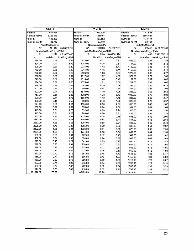
Trial 13FirstFail 887.556FirstFail noPMI 6729.449NumFail 135.329NumFail noPM 33.712
NodeMaxModePct37 101617 75.08885752
NodeMaxModePctnoPMM22 2298 6.816563835
n NodePct 4odePct noPMI1968.00 1.45 5.841894.00 1.40 5.62809.00 0.60 2.40782.00 0.58 2.32762.00 0.56 2.26798.00 0.59 2.37773.00 0.57 2.29894.00 0.66 2.65216.00 0.16 0.64201.00 0.15 0.60602.00 0.44 1.79753.00 0.56 2.23590.00 0.44 1.75199.00 0.15 0.59374.00 0.28 1.11369.00 0.27 1.09413.00 0.31 1.23413.00 0.31 1.23
1967.00 1.45 5.832183.00 1.61 6.482253.00 1.66 6.682298.00 1.70 6.822102.00 1.55 6.242064.00 1.53 6.12
339.00 0.25 1.01462.00 0.34 1.37579.00 0.43 1.72317.00 0.23 0.94299.00 0.22 0.89299.00 0.22 0.89942.00 0.70 2.79958.00 0.71 2.84930.00 0.69 2.76997.00 0.74 2.96969.00 0.72 2.87944.00 0.70 2.80
101617.00 75.09
Trial 14FirstFail 870.336FirstFail noPMI 5590.4NumFail 137.552NumFail noPM 37.149
NodeMaxModePct37 100403 72.9927591
NodeMaxModePctnoPMM5
n973.00
1043.002031.002011.002106.001817.002013.002075.00
542.00608.00
1510.001902.001553.00593.00
1104.00876.00832.00969.00
1034.001155.001204.001085.001256.001241.00
167.00324.00341.00228.00228.00213.00657.00595.00686.00745.00722.00710.00
100403.00
2106 5.669062424NodePct 4odePct noPMI
0.710.761.481.461.531.321.461.510.390.441.101.381.130.430.800.640.600.700.750.840.880.790.910.900.120.240.250.170.170.150.480.430.500.540.520.52
72.99
Trial 15FirstFail 872.58FirstFail noPMI 5891.521NumFail 134.174NumFail noPM 33.761
NodeMaxModePct37 100413 74.83789706
NodeMaxModePct noPMM
n629717
115211531272972
11671217264364888
1022835329615554528456696844838683875859547909955656562569
1848175617131735.17861796
100413.
31 1848 5.473771512NodePct 4odePct noPM
.00 0.47 1.86
.00 0.53 2.12
.00 0.86 3.41
.00 0.86 3.42
.00 0.95 3.77
.00 0.72 2.88
.00 0.87 3.46
.00 0.91 3.60
.00 0.20 0.76
.00 0.27 1.08
.00 0.66 2.63
.00 0.76 3.03
.00 0.62 2.47
.00 0.25 0.97
.00 0.46 1.82
.00 0.41 1.64
.00 0.39 1.56
.00 0.34 1.35
.00 0.52 2.06
.00 0.63 2.50
.00 0.62 2.48
.00 0.51 2.02
.00 0.65 2.59
.00 0.64 2.54
.00 0.41 1.62
.00 0.68 2.69
.00 0.71 2.83
.00 0.49 1.94
.00 0.42 1.66
.00 0.42 1.69
.00 1.38 5.47
.00 1.31 5.20
.00 1.28 5.07
.00 1.29 5.14
.00 1.33 5.29
.00 1.34 5.32
.00 74.84

Trial 16FirstFail 850.576FirstFail noPMI 6599.046NumFail 133.817NumFail noPM 32.431
NodeMaxModePct37 101386 75.76466368
NodeMaxModePctnoPMM33 1854 5.71675249
n NodePct lodePctnoPMI1102.00
967.001113.001407.001222.001207.001148.001248.00
197.00186.00522.00682.00594.00210.00
1125.001005.00
896.00907.00765.00879.00755.00792.00762.00748.00199.00299.00367.00220.00226.00152.00
1650.001674.001854.001842.001781.001728.00
101386.00
0.820.720.831.050.910.900.860.930.150.140.390.510.440.160.840.750.670.680.570.660.560.590.570.560.150.220.270.160.170.111.231.251.391.381.331.29
75.77
Trial 17FirstFail 833.52FirstFail noPMI 5498.642NumFail 137.41NumFail noPM 36.951
NodeMaxModePct37 100459 73.10894404
NodeMaxModePct noPMM23 2356
n NodePct793.00 0.58769.00 0.56640.00 0.47718.00 0.52888.00 0.65840.00 0.61752.00 0.55803.00 0.58532.00 0.39501.00 0.36
1416.00 1.031751.00 1.271614.00 1.17552.00 0.40590.00 0.43483.00 0.35506.00 0.37505.00 0.37
2060.00 1.501962.00 1.432012.00 1.462033.00 1.482356.00 1.712146.00 1.56
501.00 0.36955.00 0.70836.00 0.61614.00 0.45574.00 0.42544.00 0.40999.00 0.73889.00 0.65869.00 0.63966.00 0.70934.00 0.68
1048.00 0.76100459.00 73.11
6.376011475IodePctnoPMI
2.152.081.731.942.402.272.042.171.441.363.834.744.371.491.601.311.371.375.585.315.455.506.385.811.362.582.261.661.551.472.702.412.352.612.532.84
Trial 18FirstFail 878.424FirstFail noPMI 6482.922NumFail 136.32NumFail noPM 34.703
NodeMaxModePct37 101617 74.54298709
NodeMaxModePct noPMM
n1968.C1893.C1962.C2186.(2070.C1994.C2000.C2236.C
268.(308.(856.C
1110.0794.C306.C374.C369.C413.C413.(955.0
1190.C1314.C1337.C1127.C1014.C
339.C462.C579.C317.C299.C299.C695.C649.C608.C721.0658.(620.C
101617.0
8 2236NodePct
00 1.4400 1.3900 1.4400 1.6000 1.5200 1.4600 1.4700 1.64)0 0.2000 0.2300 0.6300 0.8100 0.5800 0.2200 0.2700 0.2700 0.3000 0.3000 0.700 0.8700 0.96D0 0.9800 0.83)0 0.740 0.2530 0.3430 0.4230 0.23O0 0.2230 0.2210 0.510 0.4830 0.4510 0.5330 0.4830 0.4530 74.54
6.443246982JodePctnoPMI
5.675.455.656.305.965.755.766.440.770.892.473.202.290.881.081.061.191.192.753.433.793.853.252.920.981.331.670.910.860.862.001.871.752.081.901.79
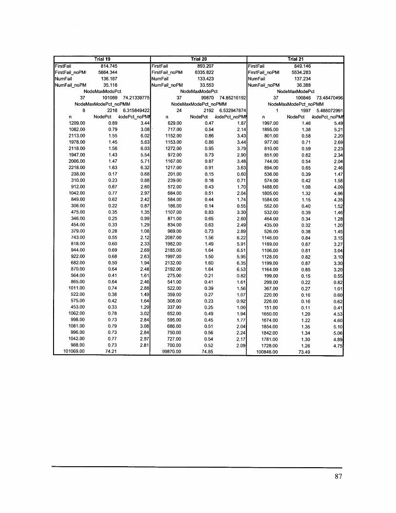
Trial 19FirstFail 814.745FirstFail noPMI 5864.344NumFail 136.187NumFail noPM 35.118
NodeMaxModePct37 101069 74.21339775
NodeMaxModePctnoPMM8 2218 6.315849422
n NodePct 4odePct noPM1209.001082.002113.001978.002118.001947.002006.002218.00
238.00310.00912.00
1042.00849.00306.00475.00346.00454.00379.00743.00818.00944.00922.00682.00870.00564.00865.00
1011.00522.00575.00453.00
1062.00998.00
1081.00996.00
1042.00988.00
101069.00
0.890.791.551.451.561.431.471.630.170.230.670.770.620.220.350.250.330.280.550.600.690.680.500.640.410.640.740.380.420.330.780.730.790.730.770.73
74.21
3.443.086.025.636.035.545.716.320.680.882.602.972.420.871.350.991.291.082.122.332.692.631.942.481.612.462.881.491.641.293.022.843.082.842.972.81
Trial 20FirstFail 893.207FirstFail noPMI 6335.822NumFail 133.423NumFail noPM 33.553
NodeMaxModePct37 99870 74.85216192
NodeMaxModePct_noPMM24 2192 6.532947874
NodePct GodePct noPMI
n629.00717.00
1152.001153.001272.00972.00
1167.001217.00201.00239.00572.00684.00584.00186.00
1107.00871.00834.00969.00
2087.001982.002185.001997.002132.002192.00
275.00541.00522.00359.00308.00337.00652.00595.00686.00750.00727.00700.00
99870.00
Trial 21FirstFail 849.146FirstFail noPMI 5534.283NumFail 137.234NumFail noPM 36.388
NodeMaxModePct37 100846 73.48470496
NodeMaxModePctnoPMM
n1997.C1895.(
801.C977.C810.C851.(744.C894.C536.C574.C
1488.01805.01584.0
552.0532.0464.0435.0526.0
1146.01189.01106.01128.01199.01164.0
199.0299.0367.0220.0226.0151.0
1650.01674.01854.01842.01781.01728.0
100846.0
1 1997 5.488072991NodePct IodePct noPMI
10 1.46 5.4910 1.38 5.2110 0.58 2.2010 0.71 2.6910 0.59 2.230 0.62 2.3410 0.54 2.0410 0.65 2.460 0.39 1.4710 0.42 1.5810 1.08 4.0910 1.32 4.9610 1.15 4.3510 0.40 1.5210 0.39 1.4610 0.34 1.2810 0.32 1.2010 0.38 1.450 0.84 3.150 0.87 3.27
)0 0.81 3.040 0.82 3.100 0.87 3.300 0.85 3.20
)0 0.15 0.550 0.22 0.820 0.27 1.010 0.16 0.600 0.16 0.620 0.11 0.410 1.20 4.530 1.22 4.60'0 1.35 5.100 1.34 5.060 1.30 4.89)0 1.26 4.70 73.49
0.470.540.860.860.950.730.870.910.150.180.430.510.440.140.830.650.630.731.561.491.641.501.601.640.210.410.390.270.230.250.490.450.510.560.540.52
74.85

Trial 22FirstFail 881.804FirstFailnoPMI 6146.805NumFail 133.516NumFail noPM 33.646
NodeMaxModePct37 99870 74.80002397
NodeMaxModePct noPMM31 1848 5.492480533
n NodePct 4odePct noPMI629.00717.00714.00800.00924.00689.00884.00861.00264.00364.00888.00
1022.00835.00329.00
1107.00871.00834.00969.00
1028.001155.001216.001079.001256.001235.00275.00541.00522.00359.00308.00337.00
1848.001756.001713.001735.001786.001796.00
99870.00
0.470.540.530.600.690.520.660.640.200.270.670.770.630.250.830.650.620.730.770.870.910.810.940.920.210.410.390.270.230.251.381.321.281.301.341.35
74.80
Trial 23FirstFail 854.883FirstFail noPMI 6535.33NumFail 133.677NumFail noPM 32.831
NodeMaxModePct37 100846 75.44005326
NodeMaxModePct noPMM
n1997.(1895.(1992.(2314.(2124.(2058.(2056.(2090.(
198.(186.(522.(682.(594.(210.(532.(464.(435.(526.(765.(879.(755.(792.(762.(748.(199.(299.(367.C220.C226.C152.C873.C900.C
1007.(1031.(1036.(
945.C100846.C
4 2314 7.048216625NodePct lodePct noPMI
00 1.49 6.0800 1.42 5.7700 1.49 6.0700 1.73 7.0500 1.59 6.4700 1.54 6.2700 1.54 6.2600 1.56 6.3700 0.15 0.6000 0.14 0.5700 0.39 1.5900 0.51 2.08)0 0.44 1.8100 0.16 0.6400 0.40 1.6200 0.35 1.4100 0.33 1.3300 0.39 1.6000 0.57 2.3300 0.66 2.6800 0.56 2.3000 0.59 2.4100 0.57 2.3200 0.56 2.2800 0.15 0.6100 0.22 0.9100 0.27 1.1200 0.16 0.67)0 0.17 0.6900 0.11 0.4600 0.65 2.6600 0.67 2.7400 0.75 3.0700 0.77 3.140 0.78 3.16
00 0.71 2.8800 75.44
Trial 24FirstFail 836.323FirstFailnoPMI 5556.292NumFail 136.98NumFail noPM 37.124
NodeMaxModePct37 99856 72.89823332
NodeMaxModePct noPMM23 2356 6.34629889
n NodePct 4odePct noPMI1077.00 0.79 2.901059.00 0.77 2.851023.00 0.75 2.761100.00 0.80 2.961253.00 0.91 3.381182.00 0.86 3.181106.00 0.81 2.981246.00 0.91 3.36
532.00 0.39 1.43501.00 0.37 1.35
1416.00 1.03 3.811751.00 1.28 4.721614.00 1.18 4.35552.00 0.40 1.49403.00 0.29 1.09312.00 0.23 0.84321.00 0.23 0.86333.00 0.24 0.90
2060.00 1.50 5.551962.00 1.43 5.292012.00 1.47 5.422033.00 1.48 5.482356.00 1.72 6.352146.00 1.57 5.78
501.00 0.37 1.35955.00 0.70 2.57836.00 0.61 2.25614.00 0.45 1.65574.00 0.42 1.55544.00 0.40 1.47639.00 0.47 1.72544.00 0.40 1.47590.00 0.43 1.59595.00 0.43 1.60647.00 0.47 1.74735.00 0.54 1.98
99856.00 72.90

Trial 25FirstFail 884.009FirstFailnoPMI 6474.539NumFail 136.079NumFail noPM 34.978
NodeMaxModePct37 101101 74.29581346
NodeMaxModePct noPMM22 2298 6.569843902
n NodePct 4odePct noPMI1968.001893.001108.001166.001056.001141.001052.001266.00268.00308.00856.00
1110.00794.00306.00571.00484.00536.00635.00
1967.002183.002253.002298.002102.002064.00234.00350.00385.00262.00214.00197.00695.00649.00608.00721.00658.00620.00
101101.00
1.451.390.810.860.780.840.770.930.200.230.630.820.580.220.420.360.390.471.451.601.661.691.541.520.170.260.280.190.160.140.510.480.450.530.480.46
74.30
Trial 26FirstFailFirstFail noPMINumFailNumFail noPM
829.2036099.675
134.38633.317
NodeMaxModePct37 101069 75.20798297
NodeMaxModePct noPMM
n12091082877809822750780840182193605721625217475346454379
1140.1195.1275.1235.1005.1267.564.865.1011.522.575.453.1844.1876.1758.1867.1740.1759.
101069.
32 1876 5.630759072NodePct 4odePct noPMI
.00 0.90 3.63
.00 0.81 3.25
.00 0.65 2.63
.00 0.60 2.43
.00 0.61 2.47
.00 0.56 2.25
.00 0.58 2.34
.00 0.63 2.52
.00 0.14 0.55
.00 0.14 0.58
.00 0.45 1.82
.00 0.54 2.16
.00 0.47 1.88
.00 0.16 0.65
.00 0.35 1.43
.00 0.26 1.04
.00 0.34 1.36
.00 0.28 1.14
.00 0.85 3.42
.00 0.89 3.59
.00 0.95 3.83
.00 0.92 3.71
.00 0.75 3.02
.00 0.94 3.8000 0.42 1.6900 0.64 2.6000 0.75 3.0300 0.39 1.5700 0.43 1.7300 0.34 1.3600 1.37 5.5300 1.40 5.6300 1.31 5.2800 1.39 5.6000 1.29 5.2200 1.31 5.2800 75.21
Trial 27FirstFailFirstFail noPMINumFailNumFail noPM
851.2535521.926
138.54137.073
NodeMaxModePct37 101468 73.24041259
NodeMaxModePctnoPMM
n718.(869.(1988.(2091.(2135.(1990.02012.(2056.(559.(608.C
1612.C1782.(1623.(521.(
1144.(873.(968.C941.(757.(770.(797.C707.C773.C834.C308.C504.0523.0306.0302.0275.0967.C1128.0910.0843.0969.0910.0
101468.0
5 2135 5.7589081NodePct lodePct noPM
00 0.52 1.9410 0.63 2.34O0 1.44 5.3610 1.51 5.6410 1.54 5.7610 1.44 5.3710 1.45 5.430 1.48 5.55
00 0.40 1.51O0 0.44 1.6410 1.16 4.3510 1.29 4.8110 1.17 4.3810 0.38 1.4110 0.83 3.0910 0.63 2.3510 0.70 2.6110 0.68 2.5410 0.55 2.040 0.56 2.080 0.58 2.1510 0.51 1.9110 0.56 2.0910 0.60 2.2510 0.22 0.8310 0.36 1.3610 0.38 1.4110 0.22 0.8310 0.22 0.8130 0.20 0.7410 0.70 2.61)0 0.81 3.0410 0.66 2.45)0 0.61 2.2710 0.70 2.6110 0.66 2.450 73.24

Trial 28FirstFail 906.069FirstFail_noPMI 11473.761NumFail 119.895NumFailnoPM 20.039
NodeMaxModePct37 99856 83.28620877
NodeMaxModePct noPMM5 888 4.43135885
n NodePct 4odePct noPMP793.00769.00640.00718.00888.00840.00752.00803.00224.00224.00494.00729.00672.00206.00403.00312.00321.00333.00813.00671.00801.00774.00834.00799.00185.00309.00306.00254.00250.00172.00639.00544.00590.00595.00647.00735.00
99856.00
0.660.640.530.600.740.700.630.670.190.190.410.610.560.170.340.260.270.280.680.560.670.650.700.670.150.260.260.210.210.140.530.450.490.500.540.61
83.29
3.963.843.193.584.434.193.754.011.121.122.473.643.351.032.011.561.601.664.063.354.003.864.163.990.921.541.531.271.250.8613.192.712.942.973.233.67
Trial 29FirstFail 889.02FirstFailnoPM 7525.982NumFail 131.399NumFail_noPM 29.782
NodeMaxModePct37 101617 77.33468291
NodeMaxModePctnoPMM
n1128.001025.001108.001166.001056.001141.001052.001266.00268.00308.00856.00
1110.00794.00306.00571.00484.00536.00635.00955.00
1190.001314.001337.001127.001014.00339.00462.00579.00317.00299.00299.00942.00958.00930.00997.00969.00944.00
101617.00
1337 4.489288832NodePct 4odePct noPMK
0.86 3.790.78 3.440.84 3.720.89 3.920.80 3.550.87 3.830.80 3.530.96 4.250.20 0.900.23 1.030.65 2.870.84 3.730.60 2.670.23 1.030.43 1.920.37 1.630.41 1.800.48 2.130.73 3.210.91 4.001.00 4.411.02 4.490.86 3.780.77 3.400.26 1.140.35 1.550.44 1.940.24 1.060.23 1.000.23 1.000.72 3.160.73 3.220.71 3.120.76 3.350.74 3.250.72 3.17
77.34I