livermore on model criteria for sampling, testing,...
TRANSCRIPT

LLNL‐TR‐669645
Recommendations on Model Criteria for Groundwater Sampling, Testing, and Monitoring of Oil and Gas Development in California
Bradley K. Esser1, Harry R. Beller2, Susan A. Carroll1, John A. Cherry3, Jan Gillespie4, Robert B. Jackson5, Preston D. Jordan2, Vic Madrid1, Joseph P. Morris1, Beth L. Parker3, William T. Stringfellow2, Charuleka Varadharajan2, and Avner Vengosh6
1Lawrence Livermore National Laboratory, Livermore, California 2Lawrence Berkeley National Laboratory, Berkeley, California 3University of Guelph, Guelph, Canada 4California State University, Bakersfield, California 5Stanford University, Stanford, California 6Duke University, Durham, North Carolina
June, 2015
Final Report California State Water Resources Control Board
State of California Contract 14‐050‐250; LLNL Work for Others Proposal L15606
LAWRENCE
N AT I O N A L
LABORATORY
LIVERMORE

Disclaimer This document was prepared as an account of work sponsored by an agency of the United States government. Neither the United States government nor Lawrence Livermore National Security, LLC, nor any of their employees makes any warranty, expressed or implied, or assumes any legal liability or responsibility for the accuracy, completeness, or usefulness of any information, apparatus, product, or process disclosed, or represents that its use would not infringe privately owned rights. Reference herein to any specific commercial product, process, or service by trade name, trademark, manufacturer, or otherwise does not necessarily constitute or imply its endorsement, recommendation, or favoring by the United States government or Lawrence Livermore National Security, LLC. The views and opinions of authors expressed herein do not necessarily state or reflect those of the United States government or Lawrence Livermore National Security, LLC, and shall not be used for advertising or product endorsement purposes.
Auspices Statement This work performed under the auspices of the U.S. Department of Energy by Lawrence Livermore National Laboratory under Contract DE‐AC52‐07NA27344.

Recommendations on Model Criteria for Groundwater Sampling, Testing, and Monitoring of Oil and Gas Development in California
Bradley K. Esser1, Harry R. Beller2, Susan A. Carroll1, John A. Cherry3, Janice M.
Gillespie4, Robert B. Jackson5, Preston D. Jordan2, Vic Madrid1, Joseph P. Morris1, Beth L. Parker3, William T. Stringfellow2, Charuleka Varadharajan2, and Avner
Vengosh6
1Lawrence Livermore National Laboratory, Livermore, California 2Lawrence Berkeley National Laboratory, Berkeley, California
3University of Guelph, Guelph, Canada 4California State University, Bakersfield, California
5Stanford University, Stanford, California 6Duke University, Durham, North Carolina
Prepared in cooperation with the California State Water Resources Control Board
LLNL‐TR‐669645
June 2015
LLNL‐TR‐669645 Esser et al. (2015)
2 Recommendations for Groundwater Monitoring Criteria under SB4
Suggested citation: Esser BK, Beller HR, Carroll SA, Cherry JA, Gillespie JM, Jackson RB, Jordan PD, Madrid V, Parker BL, Stringfellow WT, Varadharajan C, and Vengosh A, 2015, Recommendations on Model Criteria for Groundwater Sampling, Testing, and Monitoring of Oil and Gas Development in California, Lawrence Livermore National Laboratory LLNL‐TR‐669645

Esser et al. (2015) LLNL‐TR‐669645
Recommendations for Model Groundwater Monitoring Criteria under SB4 3
ContentsExecutive Summary ......................................................................................................................... 7
1 Introduction .......................................................................................................................... 16
1.1 Groundwater Monitoring Model Criteria ..................................................................... 16 1.2 Expert Advice in the Design of Model Criteria .............................................................. 17 1.3 Outline of Report .......................................................................................................... 17
2 Well Stimulation in California ............................................................................................... 19
2.1 Well Stimulation Practice in California ......................................................................... 19 2.2 Quantities of Flowback and Produced Water Generated in California and Their Current Management and Disposal Practices .......................................................................... 23 2.2.1 Introduction .............................................................................................................. 23 2.2.2 Quantities of Flowback and produced water generated in California ..................... 24 2.2.3 Management practices for flowback and produced water disposal in CA ............... 25
2.3 Contaminant release pathways resulting from well stimulation activities .................. 27 2.3.1 Normal pathways related to management and disposal of flowback/produced water (wastewater)............................................................................................................... 28 2.3.2 Potential subsurface leakage pathways ................................................................... 33 2.3.3 Surface spills and leaks ............................................................................................. 41
3 Protected Groundwater in California ................................................................................... 43
3.1 Definitions & regulatory framework ............................................................................. 43 3.2 Current state of knowledge of the distribution of 0‐3,000 mg/L and 3,000‐10,000 mg/L groundwater in California ................................................................................................ 47 3.3 Current Efforts to Map Groundwater Salinity in the San Joaquin Valley ..................... 49
4 Monitoring the Impact of Oil and Gas Development on Groundwater ............................... 54
4.1 Monitoring outside of California .................................................................................. 54 4.1.1 Review of groundwater quality sampling studies in the United States ................... 55 4.1.2 Detection of well stimulation fluids in groundwater ................................................ 57 4.1.3 Detection of direct contaminants from target formations in groundwater ............ 58 4.1.4 Stray gas contamination of groundwater ................................................................. 60
4.2 Baseline Monitoring ...................................................................................................... 62 4.2.1 Legacy issues ............................................................................................................. 62 4.2.2 Land use .................................................................................................................... 63
4.3 Well Integrity ................................................................................................................ 63 4.3.1 The Importance of Well Integrity.............................................................................. 63 4.3.2 Field observations of wellbore‐integrity failure ....................................................... 64 4.3.3 Risk of older wells to leakage .................................................................................... 65 4.3.4 Existing Well Integrity Standards in California .......................................................... 66
4.4 Site Conceptual Models ................................................................................................ 66 4.4.1 Site Conceptual Models at the Area Scale ................................................................ 70
LLNL‐TR‐669645 Esser et al. (2015)
4 Recommendations for Groundwater Monitoring Criteria under SB4
4.4.2 Site Conceptual Models at the Regional Scale ......................................................... 72 4.4.3 Conceptual Models Summary ................................................................................... 73
5 Analytes for Monitoring Groundwater ................................................................................. 75
5.1 Chemicals Used in Well Stimulation ............................................................................. 75 5.2 Chemical Use in Other Oil and Gas Development Activities ........................................ 81 5.3 Flowback and Produced Waters ................................................................................... 82 5.3.1 Characteristics of flowback fluids ............................................................................. 82 5.3.2 Characteristics of produced water............................................................................ 83
5.4 Intrinsic Tracers (Geochemical, Isotopic, and Gas Tracers) .......................................... 86 5.4.1 Hydrocarbons and noble gases ................................................................................. 86 5.4.2 Water Chemistry ....................................................................................................... 89
5.5 Introduced Tracers ........................................................................................................ 92 5.5.1 Desirable properties of added tracers for evaluating groundwater impacts of hydraulic fracturing ............................................................................................................... 92 5.5.2 Potential candidates for use as introduced tracers for evaluating groundwater impacts .................................................................................................................................. 93
5.6 Sampling Methods ........................................................................................................ 94 5.7 Detecting impact and establishing baseline ................................................................. 96
6 Recommendations for Area‐Specific Monitoring ................................................................. 99
6.1 Discussion of Recommendations for Area‐Specific Monitoring ................................... 99 6.1.1 Groundwater monitoring of well stimulation in California ...................................... 99 6.1.2 Protected groundwater .......................................................................................... 105 6.1.3 Risk‐based groundwater monitoring ...................................................................... 107 6.1.4 Groundwater monitoring design ............................................................................ 120 6.1.5 Periodic Review ....................................................................................................... 123
6.2 Summary of Recommendations for Area‐Specific Groundwater Monitoring Criteria 132 7 Recommendations for Regional Groundwater Monitoring Model Criteria ....................... 147
7.1 Goals of the Regional Groundwater Monitoring Program ......................................... 147 7.1.1 The primary goal of the Regional Groundwater Monitoring Program (RGMP) should be to be to monitor the impact of oil and gas activities on protected groundwater resources in the State. ........................................................................................................ 147 7.1.2 The RGMP should develop regional‐scale conceptual models for protected groundwaters within and adjacent to oil and gas fields. .................................................... 148 7.1.3 The RGMP should establish monitoring networks to detect transport of fluids from hydrocarbon producing zones to protected groundwater aquifers that is related to oil and gas development. ................................................................................................................ 148 7.1.4 The RGMP should characterize risks to and impacts on groundwater resources from discharge of oil and gas wastewater to surface ponds ...................................................... 149 7.1.5 The RGMP should assess the potential risk of well integrity failures and inadequate seals to protected groundwater quality statewide. ........................................................... 149
7.2 The Protected Groundwater Resource ....................................................................... 150
Esser et al. (2015) LLNL‐TR‐669645
Recommendations for Model Groundwater Monitoring Criteria under SB4 5
7.2.1 The RGMP should monitor groundwater with less than 10,000 mg/L total dissolved solids (TDS) in aquifers that contain a sufficient quantity of water for beneficial use and that are in groundwater basins containing oil and gas fields. ............................................ 150 7.2.2 The State should implement a program to systematically determine the spatial and vertical distribution of all fresh groundwater (< 3,000 mg/L TDS) and protected groundwater (< 10,000 mg/L) in basins containing oil & gas fields throughout the State. 150
7.3 Groundwater Monitoring Systems ............................................................................. 151 7.3.1 The RGMP should use or install dedicated monitoring wells to monitor protected groundwater ....................................................................................................................... 151 7.3.2 The RGMP should consider the use of idle or inactive oil and gas wells for monitoring deep protected groundwater. ......................................................................... 152 7.3.3 The RGMP should consider using existing water supply and monitoring wells for monitoring aquifers of beneficial use. ................................................................................ 152
7.4 Groundwater Quality Monitoring Constituents ......................................................... 152 7.4.1 The RGMP should monitor regulated chemical constituents, geochemical and isotopic tracers of source and transport, and anthropogenic constituents indicative of oil and gas development .......................................................................................................... 153 7.4.2 Water quality monitoring under the RGMP should be coordinated with other SB4 water quality monitoring efforts. ....................................................................................... 154 7.4.3 The RGMP should have access to injected fluid, produced water, and groundwater samples collected for chemical analysis as a part of SB4 or UIC monitoring programs ..... 155 7.4.4 All RGMP water quality data should be submitted to the Water Board in an electronic format that is compatible with the State Board’s GeoTracker GAMA database. 155
7.5 Identifying Impact of Oil and Gas Operations on Protected Groundwater Quality ... 155 7.5.1 The RGMP should use multiple lines of evidence to attribute changes in water quality to natural or anthropogenic processes ................................................................... 156 7.5.2 The RGMP should actively develop geochemical and isotopic methods to establish signatures that allow attribution of constituent sources and pathways. .......................... 156 7.5.3 The RGMP should assess the source and distribution of methane in protected groundwater aquifers ......................................................................................................... 157 7.5.4 The RGMP should assess the vulnerability of protected groundwater aquifers to potential impact by oil and gas development. ................................................................... 157
7.6 Pilot and Special Studies ............................................................................................. 157 7.6.1 The RGMP should conduct, facilitate and/or participate in focused field or pilot studies in collaboration with industry and with the assistance of a Technical Advisory Committee. ......................................................................................................................... 158 7.6.2 The RGMP should develop studies to close known data gaps; to improve monitoring of the impact of oil and gas operations on groundwater quality; and to develop better understanding of aquifer vulnerability and contaminant transport. ...................... 158
7.7 Prioritization of oil and gas fields for RGMP ............................................................... 161 7.7.1 The RGMP should prioritize monitoring groundwater within and adjacent to fields where well stimulation is currently practiced .................................................................... 161 7.7.2 The RGMP should prioritize monitoring based on vulnerability ............................ 161

LLNL‐TR‐669645 Esser et al. (2015)
6 Recommendations for Groundwater Monitoring Criteria under SB4
7.7.3 The RGMP should prioritize monitoring fresh water aquifers ............................... 162 7.7.4 The RGMP should consider existing infrastructure and knowledge in its prioritization ....................................................................................................................... 162
7.8 Regional Groundwater Monitoring Program Implementation ................................... 162 7.8.1 The RGMP should use a phased approach to the implementation of regional groundwater monitoring .................................................................................................... 162 7.8.2 The RGMP should compile existing information and develop an information management system for regional monitoring data and models ........................................ 163 7.8.3 The RGMP should periodically review and interpret RGMP data .......................... 163 7.8.4 The RGMP should establish a Technical Advisory Committee (TAC)...................... 164
8 Appendix: Experts Contributing to Recommendations ...................................................... 165
8.1 Lawrence Livermore National Laboratory .................................................................. 165 8.2 Lawrence Berkeley National Laboratory..................................................................... 167 8.3 California State University, Bakersfield ...................................................................... 169 8.4 Stanford University ..................................................................................................... 169 8.5 Duke University ........................................................................................................... 170 8.6 University of Guelph ................................................................................................... 170 8.7 Acknowledgements ..................................................................................................... 171
9 Appendix: Meetings Held .................................................................................................... 172
9.1 Public Stakeholder Meetings ...................................................................................... 172 9.2 Private Meetings ......................................................................................................... 172 9.3 Presentations at Conferences ..................................................................................... 173
10 Appendix: Current Efforts to Map Groundwater Salinity in San Joaquin Valley (Dr. Jan Gillespie) ..................................................................................................................................... 174
10.1 Chemical Analyses—Oil Wells ..................................................................................... 176 10.1.1 Quality Control .................................................................................................... 178 10.1.2 Incorporation into the GIS database .................................................................. 179
10.2 Results from DOGGR Geochemical Database Analysis ............................................... 181 10.2.1 Eastside SJV ......................................................................................................... 182 10.2.2 West Side SJV ...................................................................................................... 184 10.2.3 South SJV ............................................................................................................. 187
10.3 Geophysical Log Analysis ............................................................................................ 188 10.3.1 Resistivity Porosity (RP) Method ........................................................................ 189
10.4 Resistivity‐Porosity Method Results to Date .............................................................. 192 10.4.1 Sensitivity Analysis .............................................................................................. 193
11 Appendix: Overview of Depth‐Discrete Multilevel Groundwater Monitoring Technologies: Focus on Groundwater Monitoring in Areas of Oil and Gas Well stimulation in California ....... 197
12 References .......................................................................................................................... 278
Esser et al. (2015) LLNL‐TR‐669645
Recommendations for Model Groundwater Monitoring Criteria under SB4 7
Recommendations on Model Criteria for Groundwater Sampling, Testing, and Monitoring of Oil and Gas Development in California Bradley K. Esser, Harry Beller, Susan Carroll, John Cherry, Jan Gillespie, Rob Jackson, Preston D. Jordan, Vic Madrid, Joseph Morris, Beth Parker, William T. Stringfellow, Charu Varadharajan, and Avner Vengosh
EXECUTIVESUMMARY
California Senate Bill 4 (Pavley, 2013; hereafter referred to as “SB4”) was passed in response to public concerns about the environmental impacts of oil and gas well stimulation. A focus of these concerns was potential degradation of groundwater used as a supply for drinking water or agricultural irrigation by chemical additives injected into the subsurface during the hydrofracturing process and by chemicals associated with produced water generated by stimulated wells during oil production. SB4 was designed to address these concerns by mandating “strategic, scientifically based groundwater monitoring” of the state’s oil and gas fields.
To protect the State’s groundwater resources and to allay public concerns, the bill required that the State Water Resources Control Board (State Water Board or SWRCB) develop criteria for groundwater monitoring at scales from single well to regional. SB4 required that the criteria include guidance on the design of groundwater monitoring networks, on which water quality constituents to monitor, and on the frequency and duration of groundwater sampling. The bill also required that, in developing these model criteria, the state seek the advice of experts. This report provides expert recommendations from single wells (area‐specific) to regional groundwater monitoring model criteria.
Recommendations for Area‐Specific Groundwater Monitoring Model Criteria In this document, we use “area‐specific” monitoring to refer to both “well‐by‐well” monitoring and to monitoring of a closely spaced set of stimulated wells within a small area. The document recommends requirements for a groundwater monitoring plan for a stimulated well or for a tightly clustered set of stimulated wells. Chapter 6 contains both recommended area‐specific groundwater monitoring criteria and a discussion of these criteria. Groundwater monitoring of well stimulation in California: The challenges in designing a groundwater quality monitoring network for well stimulation in California on either an area‐specific or regional scale are enormous. Oil and gas well stimulation occurs at depths that are generally deeper than protected groundwater resources. While the stratigraphy of shallow fresh water zones and deeper oil and gas zones is often known, information relevant to contaminant transport in intervening zones is often unavailable. Oilfields are dynamic with temporally and spatially variable pressure gradients. In fields with long histories of

LLNL‐TR‐669645 Esser et al. (2015)
8 Recommendations for Groundwater Monitoring Criteria under SB4
development, legacy impacts from previous drilling, production and other operations on overlying protected groundwater resources may complicate detection of impact from current operations. These fields may also contain active, inactive or abandoned wells in close proximity to the stimulated well being monitored; and the integrity of these nearby wells may or may not be known. And to the extent that wells act as pathways for the migration of liquids and gases, all protected groundwater aquifers overlying hydrocarbon producing zones across depths of up to thousands of feet are potentially at risk. All of these factors and more combine to make designing a site‐specific and risk‐based groundwater monitoring network extremely difficult Adding to the challenge is that very few examples exist where purposeful groundwater monitoring networks have been created to assess impacts by well stimulation on the groundwater resource (e.g., Hammack et al., 2014), and no examples exist where such networks are required by a regulatory program. Several expert panel reports on the environmental impacts of shale gas development in the USA, Canada, Australia, and Europe have all have recommended groundwater monitoring, but none of the reports have indicated where and how such monitoring should be accomplished. Whatever information exists about the impacts of petroleum resource development comes from the sampling of household wells, farm wells, municipal wells, and springs. SB4 requires, however, that well‐by‐well groundwater monitoring be conducted for all new well stimulation projects. Beginning in July 2015, before a well stimulation can proceed, a groundwater monitoring plan must be submitted to and approved by the State Water Board. The challenge then is to develop a scientifically credible approach to this permit‐required monitoring in the absence of experience from similar regulatory programs elsewhere in the nation or world. Groundwater monitoring network design: The design of a groundwater monitoring network (where and how to place monitoring wells, how often to collect groundwater samples, and what to analyze) is contingent on the purpose of the groundwater monitoring. Several types of groundwater monitoring exist. A common type of groundwater monitoring for a process or source that has the potential to contaminate groundwater, but has not been demonstrated to be leaking, is termed “detection monitoring”. Landfills are often required to have detection monitoring networks in place to provide early detection of leakage. We do not recommend this type of monitoring for well stimulation in California. Such an approach requires knowledge of contaminant pathways and of local hydrology and hydrogeology in order to design a monitoring network and the installation of numerous monitoring locations to be effective. We currently don’t have such knowledge and the cost and expense of installing an early‐detection groundwater monitoring network on a well‐by‐well basis would be prohibitive. We do recognize a need for groundwater monitoring, however, and recommend monitoring and baseline characterization of protected groundwaters overlying and adjacent to stimulated well operations. The goal of this form of monitoring is not early detection of impact sufficient to identify leakage from an individual stimulation, but rather detection of current or legacy impacts related to well stimulations on a protected groundwater aquifer. Critical to

Esser et al. (2015) LLNL‐TR‐669645
Recommendations for Model Groundwater Monitoring Criteria under SB4 9
demonstrating impact is having adequate characterization of baseline water quality, including spatial and temporal variability. Establishing baseline and baseline variability is crucial for chemical constituents that occur naturally and for oil and gas related chemical constituents in areas with a long history of oil and gas development. The recent draft EPA Assessment of the Potential Impacts of Hydraulic Fracturing for Oil and Gas on Drinking Water Resources (USEPA, 2015b) states that “baseline data on local water quality is needed to quantify changes to drinking water resources and to provide insights into whether nearby hydraulic fracturing activities may have caused any detected changes” and states that a limitation of the assessment is “insufficient pre‐ and post‐hydraulic fracturing data on the quality of drinking water resources”. An additional benefit of area‐specific monitoring will be in characterizing the spatial distribution of groundwater resources with potential beneficial use. The occurrence, depth distribution, and vertical hydraulic communication of groundwaters with between 3,000 and 10,000 mg/L total dissolved solids (TDS), in particular, is poorly known. We also recommend sentry monitoring for existing water supply wells within one mile of the well stimulation through the installation of guard well(s) located between the stimulation well and the water supply well, as well as setting up to monitor the aquifers accessed by water supply wells. Protected groundwater: We recommend monitoring groundwater of less than 10,000 mg/L TDS in an aquifer that produces or could produce water in sufficient quantity for beneficial use and that is not excluded from groundwater monitoring by written concurrence from the State or Regional Water Board. California is in the midst of a historic drought and any water with the potential for beneficial use should be protected. The limit of 10,000 mg/L TDS aligns with federal regulations concerning Underground Injection Control and is technically and economically feasible to desalinate. We also recommend that area‐specific groundwater monitoring plans include information on the vertical profile of groundwater salinity in aquifers overlying the stimulated zone. Risk‐based groundwater monitoring: We recommend that monitoring of protected groundwater for impact from well stimulation consider three risk factors: the vertical separation between the base of protected groundwater and the stimulated zone, the presence of potential pathways (wells and transmissive geologic features) in close proximity to the stimulated well, and the density of previously stimulated wells in the immediate vicinity of the stimulated well (Table 6.1). We also recommend that monitoring be tiered on the basis of the quality of the groundwater being protected. We recommend monitoring higher quality water (groundwater with less than 3,000 mg/L TDS that qualifies for a municipal or domestic water supply beneficial use) more intensively than lower‐quality water (groundwater with between 3,000 and 10,000 mg/L TDS that qualifies as protected groundwater). We recommend that, for the purpose of identifying potential contaminant pathways and assessing vertical separation, a conservative estimate of the extent and orientation of fracturing

LLNL‐TR‐669645 Esser et al. (2015)
10 Recommendations for Groundwater Monitoring Criteria under SB4
during well stimulation be used, and we propose how to conservatively estimate stimulated volume (which we term the Axial Dimensional Stimulated Volume or ADSV) based on the operator‐submitted Axial Dimensional Stimulation Area (ADSA). We recommend using the conservatively defined ADSV to identify potential pathways (i.e., wells and geologic features) in close proximity to the stimulated well and to assess whether these vulnerabilities, including vertical separation, pose an unacceptable risk to protected groundwater resources. We recommend allowing the operator to propose a less conservative estimate of stimulated volume using field data relevant to stress orientation and fracture azimuth for the strata being stimulated, but reserving for the Water Board the final decision on which estimate of stimulated volume will be used. We believe that one of the more significant potential contaminant pathways is transmission through wells in close proximity to the stimulated well, especially wells that have not been adequately sealed or properly abandoned. We recommend that for wells within close proximity (2 x ADSV) to a stimulated well, the Board require cementing of the outer annular space along the entire length of casing from a regional seal or aquitard below the base of protected groundwater to the ground surface. Wells that do not meet this standard would be considered to be “likely” pathways. The density of previously stimulated wells in close proximity to the stimulated well being monitored is also a risk factor. Everything else being equal, risk to protected groundwater will scale with the density of stimulations, and the legacy stimulated well densities in California vary by orders of magnitude. Ground monitoring network configuration: In consideration of the risk factors, we recommend that all new well stimulation projects be required to monitor a low‐salinity (0‐3,000 mg/L TDS) aquifer with the highest quality water (i.e., lowest salinity), and that all new stimulation projects (with the exception of exploratory wells with no wells or geologic features in close proximity) also be required to monitor an aquifer near the base of the protected groundwater (3,000‐10,000 mg/L TDS) zone. For stimulated wells in higher density fields (i.e., wells with >50 previously stimulated wells within ½ mile), we recommend requiring monitoring of an additional third aquifer at the base of the freshwater (0‐3,000 mg/L TDS) zone. High‐quality freshwater aquifers are the most likely to be used for domestic, municipal, or agricultural water supply and are the most sensitive to degradation. Protected groundwater aquifers closest to the stimulated zone will likely be the first to be impacted by transport of injected fluids through transmissive geologic features or by upwelling or migration of formation fluids out of the hydrocarbon‐producing zone into shallower protected groundwater zones through a breach in caprock or confining layers. For proposed stimulated wells in close proximity to likely pathways, i.e., to geologic features known to be transmissive or to existing wells that cannot be demonstrated to be adequately sealed or abandoned, we recommend additional review of well integrity, site hydrogeology, and potential future use of the aquifers. Based on an assessment of risk, we recommend not

Esser et al. (2015) LLNL‐TR‐669645
Recommendations for Model Groundwater Monitoring Criteria under SB4 11
allowing well stimulation to proceed unless pre‐existing wells are adequately sealed or allowing well stimulation to proceed with monitoring of additional aquifers. For each aquifer monitored, we recommend requiring one upgradient and two downgradient locations. A single well or location rarely provides information sufficient for groundwater protection. We recommend that the locations be within ½ mile of stimulated wells with existing wells or geologic features in close proximity or within 1 mile of stimulated wells with no potential pathways in close proximity. For stimulated wells in high‐density fields (i.e., with more than 50 previously stimulated wells within ½ mile) with existing wells or geologic features in close proximity, we recommend requiring more than three monitor locations at the discretion of the Water Board. Legacy impacts in densely drilled fields may result in spatially variable water quality in protected groundwater aquifers and require more monitoring wells to adequately characterize the spatial variability. The recommendation to use one upgradient and two downgradient monitoring wells within ½ mile of the stimulated well is a minimum configuration. We recommend allowing operators to submit alternative groundwater monitoring plans when sufficient data are available to develop a credible site conceptual model. We recommend installation of either traditional monitoring wells with screens up to fifty feet in length or engineered multi‐level systems. We do not recommend the use of nested wells (multiple wells in a single borehole) because the integrity of seals between nested wells in such systems is difficult to construct and verify. Tiered Analysis of Chemical Constituents: We recommend a tiered approach to monitoring of analytes in which all groundwater samples are analyzed for a suite of chemical constituents (Tier 1 constituents) and, if statistically significant changes in water quality consistent with impact by well stimulation are observed, a second set (Tier 2) of chemical constituents are analyzed that are focused on site‐specific well stimulation chemical additives but are more analytically challenging than Tier 1 constituents. Tier 1 constituents include total dissolved solids; major and minor anions (e.g., Cl‐, Br‐, I‐, F‐) and cations (e.g., Na+, Ca2+, K+, NH4
+); trace elements (e.g., barium, boron, lithium, strontium); regulated metals and metalloids (e.g., arsenic, copper, chromium, selenium), organic compounds (e.g., benzene, toluene, ethylbenzene, xylenes, naphthalene), and radionuclides (e.g., Ra‐226, Ra‐228, uranium); methane, ethane, and propane; total petroleum hydrocarbons; the isotopic composition of carbon in methane and of hydrogen and oxygen in water; commonly measured field parameters; and indicator compounds. A key assumption is that impact by injected or produced fluids associated with well stimulations will have a detectable effect on more than one of the chemical constituents on this list. Table 6.2 discusses each class of compound and the rationale for inclusion on the Tier 1 list. The interim regulation in California required the analysis of a suitable chemical indicator of well stimulation treatment fluid but did not specify such indicators. We recommend analysis of guar gum sugars. Guar gum is commonly used in large quantity in gel‐based hydrofracture

LLNL‐TR‐669645 Esser et al. (2015)
12 Recommendations for Groundwater Monitoring Criteria under SB4
operations and analysis of guar gum sugars is simple and inexpensive. We also recommend the analysis of two additional compounds to be proposed by the operators with the concurrence of Water Board staff. One compound shall be chosen on the basis of high mass use in the stimulation well being monitored, and a second compound shall be chosen on the basis of high persistence during subsurface transport. Should chemical additives be detected or should changes in water quality consistent with impact from produced waters be observed, we recommend that samples be collected and analyzed for toxic well stimulation additives, such as biocides, alcohols and glycols, and surfactants. Additional analyses could also include other indicators of impact from well stimulation, such as the isotopic composition of carbon in dissolved inorganic carbon, the isotopic composition of dissolved lithium, boron, sulfur, and strontium; and the concentration and isotopic composition of dissolved noble gases. We recommend groundwater sampling of each monitoring well before the well stimulation and then semi‐annually for at least three years after the well stimulation. The Need for Database and a Georeferenced Repository: We recommend 1) the submission of groundwater quality data in a timely manner as Electronic Data Deliverables (EDD) and as spreadsheets to a State‐maintained database with the goal to provide transparency, and 2) that the data be easily accessible to the public and water resource community and that it support investigations, assessments and research relevant to oil and gas development impacts on groundwater quality. We also recommend the development of a publicly accessible georeferenced repository linked to the water quality data for all hydrogeologic, geologic, and geophysical data or other information gathered or submitted in area‐specific groundwater monitoring plans. The Need for Periodic Review: We recommend that the area‐specific groundwater modeling criteria be comprehensively reviewed five years after implementation. The review should consider changes in required monitoring (including the number of aquifers to be monitored; the number of monitoring locations in each aquifer; monitoring well or system construction; sampling protocols, frequency and duration; and chemical constituents to be analyzed) based on area‐specific program data and experience over the previous five years, data and results from the regional program, and field‐based pilot studies. We also recommend less comprehensive ongoing reviews to address difficulties in program implementation and unexpected results. The Need for Field‐Based Pilot Studies: Field‐focused pilot studies are required to advance the state of science sufficiently to allow more robust assessment of the risk that well stimulation poses to protected groundwater resources, to develop better metrics for assessing that risk, and to develop better approaches to monitoring impact. We strongly recommend that pilot studies be an integral component of the monitoring program and be used to inform development of the program over time.

Esser et al. (2015) LLNL‐TR‐669645
Recommendations for Model Groundwater Monitoring Criteria under SB4 13
Recommendations for Regional Groundwater Monitoring Model Criteria Goals of the Regional Groundwater Monitoring Program (RGMP) We recommend that the regional program not be restricted to monitoring the impact of well stimulation on protected groundwater resources, but should also characterize impacts from all oil and gas activities, including surface and subsurface disposal of produced wastewater.
The primary goal of the Regional Groundwater Monitoring Program (RGMP) should be to be to establish a current baseline and monitor the impact of all oil and gas activities on protected groundwater resources in the State.
The RGMP should develop regional‐scale conceptual models for protected groundwaters within and adjacent to oil and gas fields.
The RGMP should establish monitoring networks to detect transport of fluids from hydrocarbon producing zones to protected groundwater aquifers that is related to oil and gas development.
The RGMP should characterize risks to and impacts on groundwater resources from discharge of oil and gas wastewater to surface ponds
The RGMP should assess the potential risk of well integrity failures and inadequate seals to protected groundwater quality statewide.
The Protected Groundwater Resource We recommend that the regional program monitor groundwaters with less than 10,000 mg/L TDS and that the State should implement a program to systematically map this resource.
The RGMP should monitor groundwater with less than 10,000 mg/L total dissolved solids (TDS) in aquifers that contain a sufficient quantity of water for beneficial use and that are in groundwater basins containing oil and gas fields.
The State should implement a program to systematically determine the spatial and vertical distribution of all fresh groundwater (< 3,000 mg/L TDS) and protected groundwater (< 10,000 mg/L) in basins containing oil & gas fields throughout the State.
Groundwater Monitoring Systems We recommend that the regional program install or use dedicated groundwater monitoring systems and investigate the use of deep oil and gas wells for monitoring.
The RGMP should use or install dedicated wells to monitor protected groundwater, including those in other programs
The RGMP should consider the use of idle or inactive oil and gas wells as a cost‐effective tool for monitoring
The RGMP should consider using existing water supply wells for monitoring aquifers of beneficial use.
Groundwater Quality Monitoring Constituents We recommend that the constituents monitored by the regional program be coordinated with other SB4 programs, that water quality data be made available in a publicly accessible
LLNL‐TR‐669645 Esser et al. (2015)
14 Recommendations for Groundwater Monitoring Criteria under SB4
database, and that the regional program have access to produced and injected water. Characterization of the man‐made and naturally occurring chemicals in return fluids and produced water from oil and gas wells in different basins in California is essential to identifying impact in protected groundwater.
The RGMP should monitor regulated chemical constituents, geochemical and isotopic tracers of source and transport, and anthropogenic constituents indicative of oil and gas development
Water quality monitoring under the RGMP should be coordinated with other SB4 water quality monitoring efforts.
The RGMP should have access to injected fluid, produced water, and groundwater samples collected for chemical analysis as a part of SB4 or UIC monitoring programs
All RGMP water quality data should be submitted to the Water Board in an electronic format that is compatible with the State Board’s GeoTracker GAMA database.
Identifying Impact of Oil and Gas Operations on Protected Groundwater Quality We recommend using multiple lines of evidence for contaminant source attribution, assessing the current distribution of methane in protected groundwater, and assessing aquifer vulnerability through development of regional conceptual models and an improved understanding of well integrity risk factors.
The RGMP should use multiple lines of evidence to attribute changes in water quality to natural or anthropogenic processes
The RGMP should actively develop geochemical and isotopic methods to establish signatures that allow attribution of constituent sources and pathways.
The RGMP should assess the source and distribution of methane in protected groundwater aquifers
The RGMP should assess the vulnerability of protected groundwater aquifers to potential impact by oil and gas development.
Pilot and Special Studies We strongly recommend that pilot studies be an integral component of the RGMP. Significant gaps exist in our understanding of the impact of oil and gas development on groundwater resources in California and in how to monitor these impacts. Focused fields studies are absolutely vital to developing better approaches to monitoring; to assessing significant risk factors; and to developing effective mitigation strategies.
The RGMP should conduct, facilitate and/or participate in focused field or pilot studies in collaboration with industry and with the assistance of a Technical Advisory Committee.
The RGMP should develop studies to close known data gaps; to improve monitoring of the impact of oil and gas operations on groundwater quality; and to develop better understanding of aquifer vulnerability and contaminant transport. Recommended projects include
Investigating the use of inactive oil and gas production wells for groundwater monitoring.

Esser et al. (2015) LLNL‐TR‐669645
Recommendations for Model Groundwater Monitoring Criteria under SB4 15
Investigating the fate and transport of oil and gas development chemical additives and methane in groundwater
Investigating monitoring methods and defining potential impact pathways for stimulated wells.
Investigating risk from well integrity failures
Characterizing the role of aquitards in transport of water and contaminants
Prioritization of oil and gas fields for RGMP We recommend that the implementation of the RGMP be guided by a coherent and clearly stated set of priorities. California has over 500 active oil and gas fields. The recommendation to monitor the potential impact of all oil and gas operations on protected groundwaters will require substantial effort to design and implement. The criteria below are recommended for consideration in prioritizing initial efforts in the program.
The RGMP should prioritize monitoring groundwater within and adjacent to fields where well stimulation is currently practiced
The RGMP should prioritize monitoring based on vulnerability
The RGMP should prioritize monitoring fresh water aquifers
The RGMP should consider existing infrastructure and knowledge in its prioritization Regional Groundwater Monitoring Program Implementation We recommend that the RGMP use a phased approach to implement the program, compile information from all SB4 monitoring programs into an accessible database, and work closely with a scientific Technical Advisory Committee.
The RGMP should use a phased approach to the implementation of regional groundwater monitoring with due consideration to characterization and design of pathway‐specific monitoring before full implementation of ongoing monitoring.
The RGMP should compile existing information and develop an information management system for regional monitoring data and models
The RGMP should periodically review and interpret RGMP data
The RGMP should establish a Technical Advisory Committee (TAC)

LLNL‐TR‐669645 Esser et al. (2015)
16 Recommendations for Groundwater Monitoring Criteria under SB4
1 INTRODUCTION1.1 GroundwaterMonitoringModelCriteria In California Senate Bill 4 (Pavley, 2013; hereafter referred to as “SB4”), the California legislature found and declared that protecting the state’s groundwater for beneficial use, particularly sources and potential sources of drinking water, is of paramount concern. Access to safe drinking water is a major issue for California, especially to its disadvantaged communities. State policy is that every human being has the right to safe, clean, affordable, and accessible water adequate for human consumption, cooking, and sanitary purposes (Chapter 524, Statutes of 2012 (Assembly Bill 685, Eng)). SB4 further found and declared that strategic, scientifically based groundwater monitoring of the state’s oil and gas fields is critical to allaying the public’s concerns regarding well stimulation treatments of oil and gas wells.
To protect the State’s groundwater resources and to allay public concerns, the bill required that the State Water Resources Control Board (State Water Board or SWRCB) develop groundwater monitoring model criteria to assess the potential effects of well stimulation treatments and to be implemented across a range of spatial sampling scales from well‐by‐well to regional. The groundwater monitoring model criteria (referred to as “Model Criteria”) have been incorporated into California Water Code section 10783. SB4 required that the criteria include
(1) An assessment of the areas to conduct groundwater quality monitoring and their appropriate boundaries.
(2) A list of the constituents to measure and assess water quality. (3) The location, depth, and number of monitoring wells necessary to detect groundwater
contamination at spatial scales ranging from an individual oil and gas well to a regional groundwater basin including one or more oil and gas fields.
(4) The frequency and duration of the monitoring. (5) A threshold criterion indicating a transition from well‐by‐well monitoring to a regional
monitoring program. (6) Data collection and reporting protocols.
And the groundwater monitoring criteria were to consider the following factors:
(1) The existing quality and existing and potential use of all groundwater that is consistent with USEPA’s definition of an Underground Source of Drinking Water as containing less than 10,000 milligrams per liter total dissolved solids.
(2) Groundwater that is not a source of drinking water consistent as defined above. (3) Proximity to human population, public water service wells, and private groundwater
use, if known. (4) The presence of existing oil and gas production fields, including the distribution, physical
attributes, and operational status of oil and gas wells therein. (5) Events, including well stimulation treatments and oil and gas well failures, among
others, that have the potential to contaminate groundwater, appropriate monitoring to

Esser et al. (2015) LLNL‐TR‐669645
Recommendations for Model Groundwater Monitoring Criteria under SB4 17
evaluate whether groundwater contamination can be attributable to a particular event, and any monitoring changes necessary if groundwater contamination is observed.
The language of the bill makes it apparent that monitoring of groundwater that is or has the potential to be a source of drinking water is a priority but the monitoring should also consider the protection of water designated for any beneficial use. In practice, Model Criteria outline the methods to be used for sampling, analytical testing, and reporting of water quality associated with oil and gas well stimulation activities and address:
Groundwater monitoring to be conducted by oil and gas well operators;
Requirements for designated contractor sampling and testing; and
Methods for conducting a regional groundwater monitoring program to be implemented by the State Water Resources Control Board (State Water Board).
1.2 ExpertAdviceintheDesignofModelCriteria SB4 explicitly required that in the design of the Model Criteria the State Water Board seek the advice of experts. This document outlines expert recommendations for Model Criteria for groundwater monitoring in areas of oil and gas development, including in areas of oil and gas well stimulation. These recommendations cover both area‐specific groundwater monitoring to be conducted by oil and gas well operators and regional groundwater monitoring to be implemented by the State Water Board. In seeking expert advice, the State Water Board contracted with Lawrence Livermore National Laboratory (LLNL) to prepare recommendations for Model Criteria using both internal and external expertise. In developing recommendations, LLNL subcontracted with experts from academia (California State University, Bakersfield; Duke University; Stanford University; University of Guelph) and the national laboratories (Lawrence Livermore National Laboratory; Lawrence Berkeley National Laboratory), and sought input from various stakeholder groups. Short biographies and contact information for the experts consulted are in the Section 8 Appendix: Experts Contributing to Recommendations. In addition to weekly teleconferences involving only the experts, a number of meetings were held to solicit guidance from the State Water Board on the advice they were seeking as well as input from environmental and industry stakeholder groups. These meetings are listed in the Section 9 Appendix: Meetings Held.
1.3 OutlineofReport The report begins with relevant background discussions and ends with specific recommendations for area‐specific and regional monitoring. Chapter 2 – Well Stimulation in California. This chapter describes the practice of well stimulation in the State of California and potential contaminant release pathways that could

LLNL‐TR‐669645 Esser et al. (2015)
18 Recommendations for Groundwater Monitoring Criteria under SB4
affect groundwater quality, including surface spills and leaks, management and disposal of flowback and produced water, and subsurface pathways such a leakage through hydraulic fractures or through wellbores. Chapter 3 – Protected Groundwater in California. This chapter provides an overview on the current state of knowledge of the distribution of protected groundwater in California, with specific reference to waters between 0 and 3,000 mg/L total dissolved solids (TDS) and waters between 3,000 and 10,000 mg/L TDS. Chapter 4 – Monitoring the Impact of Oil and Gas Development on Groundwater. This chapter provides an overview of monitoring groundwater quality for impact from oil and gas development, and includes sections on monitoring efforts outside of California, the need for baseline monitoring, the importance of well integrity, and site conceptual models. Chapter 5 – Analytes for Monitoring Groundwater. This chapter provides an overview of chemicals used in well stimulation and in other oil and gas operations, the characteristics of produced waters, intrinsic and extrinsic tracers and statistical methods for detecting impact. Chapter 6 – Recommendations for Area‐Specific Monitoring. This chapter contains recommendations for operator‐required area‐specific monitoring, and includes a discussion of the recommendations. Chapter 7 – Recommendations for Regional Monitoring. This chapter contains recommendations for the regional groundwater monitoring program (RGMP). Each recommendation is followed by a short explanatory paragraph. Chapter 8 – Appendix: Experts Contributing to Recommendations. This appendix contains short biographies and contact information for internal and external experts who assisted LLNL in the development of these recommendations. Chapter 9 – Appendix: Meetings Held. This appendix lists public and private meetings held during the course of recommendation development. Chapter 10 ‐ Appendix: Current Efforts to Map Groundwater Salinity in San Joaquin Valley. This chapter is a technical appendix by Dr. Jan Gillespie and describes her research into defining the base of fresh water at 3,000 mg/L and of protected groundwater at 10,000 mg/L in the San Joaquin Valley. Chapter 11 – Appendix: Overview of Depth‐Discrete Multi‐level Groundwater Monitoring. This chapter is a technical appendix by Drs. John Cherry, Dr. Beth Parker and others and provides an updated review of multi‐level groundwater monitoring with special reference to groundwater monitoring of oil and gas operations in California.

Esser et al. (2015) LLNL‐TR‐669645
Recommendations for Model Groundwater Monitoring Criteria under SB4 19
2 WELLSTIMULATIONINCALIFORNIA
2.1 WellStimulationPracticeinCalifornia Well stimulation treatment (WST) is defined in California as “any treatment of a well designed to enhance oil and gas production or recovery by increasing the permeability of the formation” (Cal. Pub. Res. Code § 3157‐3158). WST includes hydraulic fracturing and acid well stimulation. Acid well stimulation includes matrix acidizing and acid fracturing. WST does not include routine use of acid for well maintenance. Hydraulic and acid fracturing involves injecting fluid into a well at a sufficiently high pressure to open a fracture in the geologic material around the well, referred to as “the formation” in the above definition. The pressure applied is higher than the stress pushing the geologic material together, such as due to its own weight combined with Poisson effects and tectonic strains, plus the strength of the material that holds it together in the absence of stress, such as due to cementing between grains in a sedimentary rock. After the injection pressure is stopped, fractures that have opened tend to close again due to the natural stresses pushing the geologic material together. As the goal of fracturing this material is to create transmissive features to increase the flow of oil and/or gas to the well, the fracturing fluids are designed to keep the fractures open to some extent after the injection stops. In hydraulic fracturing, this is accomplished by mixing a granular material, such as sand, into the injected fluid as the fracturing process proceeds. After the injection stops, the sand remains in the fracture preventing its complete closure. The fluid used in acid fracturing accomplishes this goal by etching (partially dissolving) the walls of the fracture. This process results in the physical configuration of the walls of the fracture no longer “mating” or matching when the fracture closes, resulting in portions of the fracture remaining open. Matrix acidizing involves the injection of acid at pressures lower than would result in the formation of a fracture. This approach increases the permeability of the formation by dissolving a portion of the geologic materials along the natural pores and fractures in the geologic material. Acid stimulation is most effective in carbonate rocks, such as limestone or dolomite. This is in part because the dissolution reaction in such rocks proceeds sufficiently rapidly to alter permeability during the amount of time over which it is feasible to conduct a WST. Acid stimulation can be applied in rocks consisting primarily of silicate minerals, such as quartz, feldspar, and clay minerals, but it is less effective because the dissolution of these rocks is slower. Figure 2,1 shows the number of notices approved by the California Division of Oil, Gas, and Geothermal Resources (DOGGR) by month received for the first fourteen months of during
LLNL‐TR‐669645 Esser et al. (2015)
20 Recommendations for Groundwater Monitoring Criteria under SB4
which notices were required. Hydraulic fracturing is the most commonly applied type of well stimulation. The number of notices submitted declined substantially after the first month due to adjustments by DOGGR in groundwater monitoring requirements for well stimulation. The number of notices subsequently increased as operators adjusted to these new requirements, reaching an average of about 150 per month from August through October 2014. CCST (Long et al., 2015) found that oil production from several reservoirs in California commenced in the late 1970s and early 1980s due to the application of hydraulic fracturing, and estimated the average number of operations per month ranged from 125 to 175 during the decade prior to Figure 2.1. However, Figure 2.1 shows the number of hydraulic fracturing notices declined after October, 2015, likely due to the large decline in the price of oil. Acid stimulation is used less frequently than hydraulic fracturing in California because the vast majority of WST target zones are not in carbonate rocks but rather in siliceous shales, including diatomite, porcellanite and chert, and tight sandstones. Matrix acidizing is applied less frequently, with approximately five notices per month submitted on average during the first fourteen months. Only two acid fracturing notices have been approved by the California Division of Oil, Gas, and Geothermal Resources (DOGGR). (Note that three hydraulic fracturing notices were submitted on December 31, 2013 with acid and no proppant, suggesting these were acid fracturing operations. The well stimulation completion reports available from DOGGR indicate these operations included proppant concentrations indicative of typical hydraulic fracturing operations, rather than acid fracturing.) Figure 2.2 shows the distribution of hydraulic fracturing notices by field approved by the DOGGR during the first fourteen months during which notices were required. All of the notices are for operations in onshore oil fields. Over 95% of the notices were for operations in four fields in the southwestern San Joaquin sedimentary basin: North and South Belridge, Lost Hills, and Elk Hills. To date, nearly all WSTs in California have targeted “migrated oil” in the complexly folded and faulted Miocene Monterey Formation or its stratigraphic equivalents, rather than flat‐lying, “source oil” typical of the Bakken Formation in the Williston Basin. The vast majority of California WSTs have been at depths less than 5,000 feet (Figure 2.3). Notices were approved in only two fields outside of the San Joaquin basin, both in the Ventura basin. The notices indicate 2% of the 1,532 wells planned for stimulation are horizontal, meaning the well interval from which oil is produced is nearly horizontal. Three quarters of these notices were for wells in the Rose field. Almost all the remaining wells to be stimulated are listed as directional. A review of a sampling of records for wells listed as directional indicates their producing intervals are almost always nearly vertical. The directional (off-vertical) portion of the well is between the ground surface and the producing interval. This allows the well to produce from a map location aside from where it is drilled, which offers flexibility with regard to the placement of the well pad on the ground surface.

Esser et al. (2015) LLNL‐TR‐669645
Recommendations for Model Groundwater Monitoring Criteria under SB4 21
Figure 2.1. (a) The number of well stimulation notices approved by DOGGR by month received and price of California oil at first sale from the Energy Information Administration. (b) The percentage and number of well stimulation notices approved by DOGGR by oil field.

LLNL‐TR‐669645 Esser et al. (2015)
22 Recommendations for Groundwater Monitoring Criteria under SB4
Figure 2.2. The percent of hydraulic fracturing notices approved by DOGGR that occur in each oil field. Table 2.1 provides the average water use per operation from the 731 well stimulation disclosure reports available from DOGGR on April 21, 2015. This is slightly less than half of the notices available on the same date. Water suitable for irrigation or domestic purposes was used for 90% of the stimulations. However, these operations only used 70% of the total water volume because they were smaller than the other operations. While only 2% of operations were in horizontal wells, 14% of water use occurred in these wells. This is in part because the treatment interval length in horizontal wells is five times longer than in other wells according to the completion reports (discounting reports that list the starting interval depth as 0 feet). Horizontal wells stimulate a significantly larger volume of rock compared with a typical vertical well. All 17 of the matrix acidizing operations used ammonium fluoride in combination with hydrochloric acid, which forms hydrofluoric acid when mixed. Hydrofluoric acid dissolves silicate minerals, such as are predominant in reservoirs with oil in California.
Esser et al. (2015) LLNL‐TR‐669645
Recommendations for Model Groundwater Monitoring Criteria under SB4 23
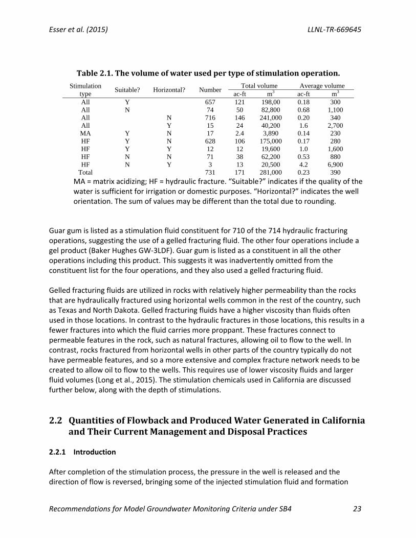
Table2.1.Thevolumeofwaterusedpertypeofstimulationoperation.
Stimulation type
Suitable? Horizontal? Number Total volume Average volume
ac-ft m3 ac-ft m3 All Y 657 121 198,00 0.18 300 All N 74 50 82,800 0.68 1,100 All N 716 146 241,000 0.20 340 All Y 15 24 40,200 1.6 2,700 MA Y N 17 2.4 3,890 0.14 230 HF Y N 628 106 175,000 0.17 280 HF Y Y 12 12 19,600 1.0 1,600 HF N N 71 38 62,200 0.53 880 HF N Y 3 13 20,500 4.2 6,900
Total 731 171 281,000 0.23 390 MA = matrix acidizing; HF = hydraulic fracture. “Suitable?” indicates if the quality of the water is sufficient for irrigation or domestic purposes. “Horizontal?” indicates the well orientation. The sum of values may be different than the total due to rounding.
Guar gum is listed as a stimulation fluid constituent for 710 of the 714 hydraulic fracturing operations, suggesting the use of a gelled fracturing fluid. The other four operations include a gel product (Baker Hughes GW‐3LDF). Guar gum is listed as a constituent in all the other operations including this product. This suggests it was inadvertently omitted from the constituent list for the four operations, and they also used a gelled fracturing fluid. Gelled fracturing fluids are utilized in rocks with relatively higher permeability than the rocks that are hydraulically fractured using horizontal wells common in the rest of the country, such as Texas and North Dakota. Gelled fracturing fluids have a higher viscosity than fluids often used in those locations. In contrast to the hydraulic fractures in those locations, this results in a fewer fractures into which the fluid carries more proppant. These fractures connect to permeable features in the rock, such as natural fractures, allowing oil to flow to the well. In contrast, rocks fractured from horizontal wells in other parts of the country typically do not have permeable features, and so a more extensive and complex fracture network needs to be created to allow oil to flow to the wells. This requires use of lower viscosity fluids and larger fluid volumes (Long et al., 2015). The stimulation chemicals used in California are discussed further below, along with the depth of stimulations.
2.2 QuantitiesofFlowbackandProducedWaterGeneratedinCaliforniaandTheirCurrentManagementandDisposalPractices
2.2.1 Introduction After completion of the stimulation process, the pressure in the well is released and the direction of flow is reversed, bringing some of the injected stimulation fluid and formation

LLNL‐TR‐669645 Esser et al. (2015)
24 Recommendations for Groundwater Monitoring Criteria under SB4
water to the surface. There are several definitions of the term “flowback” fluids (EPA, 2015). For this report, we use the operational definition of “flowback”, i.e. the initial flows in the period immediately after well stimulation but prior to production. The term “produced” water refers to long‐term flows associated with commercial hydrocarbon production. In California, the recent regulations from DOGGR introduce the term “recovered fluids”, which is defined as the water returned “following the well stimulation treatment that is not otherwise reported as produced water,” which is presumably flowback water (California DOGGR, 2013). According to one California operator, the recovered fluids can be a mixture of water from the formation, returned stimulation fluids, and well clean‐out fluids (pers. comm., Nick Besich, Aera Energy). Some data is starting to emerge about the volumes and compositions of the recovered fluids. In some cases, little to no recovered fluids are produced since the operators divert the returned flow directly into the production pipeline. Furthermore, the flowback and produced water are “commingled and co‐disposed, making separation of the stimulation fluids from the produced water impossible” (California DOGGR, 2013). Thus produced water from stimulation operations in California will likely contain some amount of returned stimulation fluid additives or their degradation products. The following sections describe the information known about the quantities of and management practices for flowback and produced waters in California. The composition of flowback and produced waters are discussed in a later chapter of this report (Section 5.3). 2.2.2 Quantities of Flowback and produced water generated in California As of 2014, operators have submitted data on the volumes of recovered fluids (i.e. flowback fluids) collected to DOGGR. Data on volumes of produced water generated are available in the DOGGR production database from 1977 onwards. The volume of recovered fluids that have been reported in 2014 were small, ranging from 0 to approximately 10,000 barrels (0 to 1,600 m3).The recovered fluid volumes were a small fraction of the injected fracturing fluid volumes (typically <5%) for hydraulic fracturing jobs, but were higher (~50‐60%) for matrix acidizing treatments (Stringfellow et al., 2015). The recovered fluids were also equivalent to a small fraction (typically <1%) of the produced water generated in the first month of operation. These results combined suggest that there is some fraction of stimulation fluids present in the produced water from fracturing jobs (Stringfellow et al., 2015). Large quantities of produced water are generated in California. For example, data from the DOGGR production database show that approximately 3 billion barrels (0.5 billion m3) of produced water was generated annually between 2011 and 2013. The data indicate that in general there are no substantive differences between the volumes of produced water generated from stimulated wells and non‐stimulated wells, although there is some variance in the data (Stringfellow et al., 2015).

Esser et al. (2015) LLNL‐TR‐669645
Recommendations for Model Groundwater Monitoring Criteria under SB4 25
2.2.3 Management practices for flowback and produced water disposal in CA Note: Material for the management practices section includes contributions from and data compiled by Heather Cooley and Matt Heberger (Pacific Institute) In California, flowback fluids (also known as recovered fluids) are typically stored in tanks or pits at the well site prior to disposal. However, according to a DOGGR whitepaper, “when well stimulation occurs, most of the fluid used in the stimulation is pumped to the surface along with the produced water, making separation of the stimulation fluids from the produced water impossible. The stimulation fluid is then co‐disposed with the produced water” (California DOGGR, 2013).
Figure 2.3. Comparison of produced water disposal methods for wells in predominantly hydraulically‐fractured and non‐fractured pools in California (Jan 1, 2011 ‐ Jun 30, 2014). Data sources: DOGGR Production Injection Database and Appendix N (Long et al., 2015). Note: Subsurface injection includes injection into Class II disposal wells as well as injection for beneficial use in oil production (water flooding or steam injection). Monthly data on disposal of produced water are available in the DOGGR Production database for most wells in California from 1977 to the present. The disposition of produced water from predominantly hydraulically‐fractured pools and predominantly non‐fractured pools are shown in Figure 2.3. Predominantly fractured pools are those for which more than half the wells

LLNL‐TR‐669645 Esser et al. (2015)
26 Recommendations for Groundwater Monitoring Criteria under SB4
starting production and injection from 2002 through late 2013 are estimated to be hydraulically fractured (Appendix N, Long et al., 2015). Typically, predominantly fractured pools were developed almost entirely using hydraulic fracturing, while predominantly non‐fractured pools had almost no fracturing operations reported (Long et al., 2015). Note: Subsurface injection includes injection into Class II disposal wells as well as injection for beneficial use in oil production (water flooding or steam injection). Notably, “evaporation‐percolation” is the most common disposal method for produced water from wells in pools that are predominantly hydraulically fractured; 39% of the produced water from these pools was disposed into pits between January 2011‐June 2014 (Figure 2.3, Stringfellow et al., 2015). Almost all of the disposal to pits is to unlined pits, which are intended to primarily percolate the disposed water. These pits are referred to as produced water disposal pits, disposal ponds, sumps or surface impoundments by various state agencies. Disposal by evaporation in lined sumps is not a common practice in California (it comprised 0.001% of produced water disposal in hydraulically fractured pools and 0.05% for other pools). Disposal of produced water from predominantly hydraulically fractured pools in percolation pits was limited to Kern County (Stringfellow et al., 2015). In fact, the difference in the disposal methods between the two pool categories can be attributed to the fact that most of the hydraulic fracturing takes place in Kern County where disposal into unlined pits is a common produced water disposition practice. Subsurface injection into Class II wells is the most commonly reported disposition method for wells in pools that are not predominantly hydraulically fractured (Figure 2.3). It is the second most common disposition method for produced water from predominantly hydraulically‐fractured pools. Class II wells include disposal wells, waterflood wells, enhanced oil recovery wells, and hydrocarbon storage wells (USEPA, 2014a). The first three categories are wells used in the disposition of produced water. Disposal wells are intended to inject into permeable zones that do not contain protected groundwater strictly for the purpose of disposing of produced water. Injection of produced water into an oil reservoir serves multiple purposes, including enhancing product recovery, preventing subsidence, and disposing of produced water generated during production. As shown in Figure 2.3, a small amount (2%) of produced water in the state is discharged into surface water bodies. A smaller amount (1%) of produced water is also disposed of in sewer systems. The disposition method for some of the produced water (22% in predominantly hydraulically‐fractured pools and 15% in other pools) is either not known or not reported. “Other” was a common disposition method reported by operators – accounting for 19% of the produced water from wells in predominantly hydraulically‐fractured pools. DOGGR staff state that some operators are using the “other” category to describe disposition that is, in fact, included in some of the other categories, e.g., subsurface injection, surface body of water, sewer disposal, etc. (Stringfellow et al., 2015). Some disposition methods, however, are not explicitly covered in these categories, such as reuse for well stimulation, irrigation or other non‐industrial beneficial purposes.

Esser et al. (2015) LLNL‐TR‐669645
Recommendations for Model Groundwater Monitoring Criteria under SB4 27
It should be noted that operators have suggested these data may not reflect current operating practice. Chevron, for example, states that the data it submitted to the DOGGR indicating disposal of produced water from its operations in the Lost Hills field into percolation pits were actually incorrectly coded records, and that it had ceased disposing produced water in this manner in 2008 (Stringfellow et al., 2015). Data collected pursuant to SB 1281 will facilitate the development of a more detailed understanding of the disposition of produced water statewide.
2.3 Contaminantreleasepathwaysresultingfromwellstimulationactivities
Material for the contaminant release pathways section is drawn from CCST (2014) and includes contributions from Heather Cooley (Pacific Institute) and Matt Reagan (LBNL). Recent assessments of impacts to water quality due to well stimulation identified several potential release mechanisms and transport pathways that could lead to potential contamination of groundwater (CCST et al., 2014; Stringfellow et al., 2015). The pathways were classified as:
Normal pathways (High priority) o Pathways, related to ongoing practices for the management and disposal of
flowback and produced water that are part of routine oil and gas operations. These pathways include seepage from disposal into percolation pits, injection through Class II wells into aquifers, reuse of inadequately treated produced water for beneficial purposes, and disposal of produced water into sewer systems draining to facilities that cannot sufficiently treat the water.
Accidental pathways (Medium priority unless indicated otherwise) o Potential subsurface leakage pathways – specifically hydraulic fractures, the
stimulated well itself, nearby existing oil or gas wells (production, disposal and old/abandoned wells), and natural subsurface features such as faults, fractures, or permeable overburden.
o Surface spills and leaks of fracturing fluids and flowback/produced water during transport, production and disposal
o Accidents resulting from operator error (Low priority)
Intentional pathways (Low priority) o Unauthorized or unpermitted releases that include illegal discharges
The following sections provide further detail on each of these pathways and, whenever possible, evidence of leakage via each pathway. It should be noted that leakage via subsurface pathways is difficult to detect because 1) the release mechanisms and transport pathways are not visible; 2) there are many sources of and pathways for contaminants present in

LLNL‐TR‐669645 Esser et al. (2015)
28 Recommendations for Groundwater Monitoring Criteria under SB4
groundwater, and definitively attributing potential impacts to well stimulation is difficult; and (3) the impacts on groundwater may not be detected on relatively short time scales. The detection of these impacts is especially difficult when baseline water quality data are absent, and when there is incomplete information about the full composition of stimulation fluids and standard analytical methods to detect the chemical additives and their degradation products. 2.3.1 Normal pathways related to management and disposal of flowback/produced water
(wastewater) In California, produced water and flowback water are managed together (Section 2.2). Produced water from well stimulation is typically managed or disposed by percolation in unlined surface impoundments or injection in Class II wells (for disposal or reuse in production). In some cases the produced water can be reused for non‐industrial beneficial uses (i.e. other than for oil and gas production), and in a few instances released into sewer systems. The contaminant release pathways associated with each of these management/disposal methods are listed below.
2.3.1.1 Disposal in unlined surface impoundments In California, wastewater from oil and gas operations can be disposed by percolation in unlined pits. According to data in the DOGGR production database, nearly 2 billion barrels (0.3 million m3) of the produced water from all oil and gas operations in California were disposed into evaporation‐percolation pits between January 2011 and June 2014. As discussed in section 2.2, almost all the pits were unlined, and hence are potential pathways for transport of produced water and its constituents, including returned stimulation fluids, into groundwater. Disposal pits in California are primarily regulated by the state’s nine Regional Water Quality Control Boards. Each Regional Board is required to formulate and adopt water quality control plans, or basin plans, for all areas within the region. Most of the disposal pits occur within the jurisdiction of the Central Valley Regional Water Quality Control Board, and the locations of these pits have been recently compiled by the Board (Holcomb, 2015). Nearly 1000 disposal pits are present in the region; approximately 60% of those pits are currently active, but 36% of the active pits have illegal discharges and are operating without appropriate permits (Stringfellow et al., 2015). Disposal of oil field wastewater in percolation pits overlying groundwater with existing and future beneficial uses has thus far been permitted if the electrical conductivity (EC) (represents salinity) of the wastewater is less than or equal to 1,000 micromhos per centimeter (µmhos/cm), and a maximum of 200 milligrams per liter (mg/L) chlorides, and 1 mg/L boron. There was previously no other testing required for, or limits on, other potential contaminants. Oil field wastewater that exceeds these specified salinity limits could have been discharged in

Esser et al. (2015) LLNL‐TR‐669645
Recommendations for Model Groundwater Monitoring Criteria under SB4 29
“unlined sumps, stream channels, or surface water if the discharger successfully demonstrates to the Regional Water Board in a public hearing that the proposed discharge will not substantially affect water quality nor cause a violation of water quality objectives (California CVRWQCB, 2004). The extent to which produced water exceeding these thresholds have been disposed in the unlined pits is unknown. The Central Valley Regional Water Quality Control Board implemented an order on April 1, 2015 requiring 77 operators to conduct a chemical analysis of wastewater disposed in active produced water disposal ponds in the Central Valley; however, the list of constituents to be analyzed does not include any indicators for stimulation fluid constituents (Appendix B, California CVRWQCB, 2015). There is evidence of groundwater contamination from percolation pits used for disposal of produced water in California. For example, the Central Valley Regional Water Quality Control Board determined that several percolation pits in Lost Hills and North and South Belridge had impacted groundwater and the pits were eventually closed (California CVRWQCB, 2013a; California CVRWQCB, 2013b). There is also evidence of groundwater contamination associated with disposal of produced water in earthen percolation pits in other parts of the United States. Kell (2011) reviewed incidents of groundwater contamination caused by oil field activities in Texas between 1993 and 2008 and in Ohio between 1983 and 2007. Of the 211 incidents in Texas over the 16‐year study period, more than 35% (or 75 incidents) were associated with wastewater management and disposal activities. Fifty‐seven of these incidents were associated with produced water disposal pits, which were no longer permitted for new locations beginning in 1969 and were closed by 1984. Of the 185 groundwater contamination incidents in Ohio over the 25‐year period, 5% (or 10 incidents) were associated with the failure of unlined pits. Like Texas, earthen pits are no longer in use in Ohio, and no incidents have been reported since the mid‐1980s. Kell (2011) further notes that while there are cases of groundwater contamination incidents associated with Class II injection operations, “documented groundwater contamination incidents dropped significantly after subsurface injection replaced earthen pit disposal as the primary method of produced water management.” While these studies and others linking unlined surface impoundments to groundwater contamination do not specify whether well stimulation fluids were the cause of the contamination, they are illustrative of the hazards of this disposal method. A case in Pavillion, WY, raises additional concerns about the use of percolation pits to contain flowback and produced water. The Pavillion gas field is located in central Wyoming in the Wind River Basin, the upper portion of which serves as the primary source of drinking water for the area. Oil and gas exploration began in the area in the 1950s and increased dramatically between 1997 and 2006. In 2008, domestic well owners began complaining about taste and odor problems, and residents believed these issues to be linked to nearby natural gas activities. In response to complaints from local residents, the US EPA initiated an investigation, collecting water samples from residential, stock, shallow monitoring, deep monitoring, and two municipal wells. According to the US EPA draft report, released in 2011, high concentrations of hydraulic fracturing chemicals found in shallow monitoring wells near surface pits “indicate that pits represent a source of shallow ground water contamination in the area” (DiGiulio et al., 2011). At least 33 surface pits were used to store/dispose of drilling muds, flowback, and produced

LLNL‐TR‐669645 Esser et al. (2015)
30 Recommendations for Groundwater Monitoring Criteria under SB4
water in the area. These findings were not contested by Encana Oil and Gas, the company responsible for the natural gas wells, or other the stakeholders (Folger et al., 2012).
2.3.1.2 Injection into Class II Wells for reuse in oil and gas production or disposal The majority of produced water from oil and gas operations in California is injected into Class II wells (Section 2.2). For example, a total of 6.7 billion barrels (1 million m3) of produced water from all oil and gas operations in California was injected into Class II wells between January 2011 and June 2014. Class II wells are used to inject brines and other fluids associated with oil and gas production, and include disposal wells, enhanced recovery wells (e.g., steam flooding), and hydrocarbon storage wells (USEPA, 2014a). Of the more than 30,000 Class II wells in California, about 95% are used for enhanced oil production and ~3% are used for disposal. More than 80% of Class II wells are located in District 4, representing Kern, Inyo, and Tulare Counties (Walker, 2011). Although injection into Class II wells has been recommended as a safer method of wastewater disposal elsewhere (Kell, 2011), in California, there has been recent controversy due to the injection of produced water into federally protected waters (waters with TDS<10,000 mg/L). As of March 2015, DOGGR is reviewing 176 Class II wells that were found to be injecting into zones containing water with TDS<3000 mg/L (California DOGGR, 2015). Twenty three of those wells (22 in Kern County and 1 in Tulare County) have been shut down as of March 2015, of which two have been authorized to resume operations. The State Water Board staff identified 108 water supply wells located within a one‐mile radius of 11 of the wells that were originally shut down in July 2014. Subsequent sampling found no sign of contamination from oil and gas operations (California SWRCB, 2014). The schedule for state review and aquifer exemption process are described in a document from the U.S. EPA to the state (Bohlen and Bishop, 2015). The shallow depth of many wastewater disposal wells in California suggests why some are currently under review for potential injection into protected groundwater. Figure 2.4 shows the distribution of measured depths for a subset of wastewater disposal wells for which DOGGR provides the measured depth. This subset represents approximately 20% of all active wastewater disposal wells. Figure 2.4 indicates the majority of these wells inject at depths shallower than 2,000 ft. Figure 2.4 also shows the shallowest injection perforations for wells with a measured depth >5,999 feet. These depths were collected from well records. A comparison of the two distributions (measured depth versus measured depth for shallower wells and shallowest perforation depths for deeper wells) indicates the depth distribution of the injection intervals is potentially considerable shallower than the measured depth distribution. For instance, one well with a measured depth of 8,557 feet has a shallowest injection perforation depth of 1,240 ft. A difference of this magnitude typically occurs when a production or exploration wells is recompleted as a wastewater disposal well.
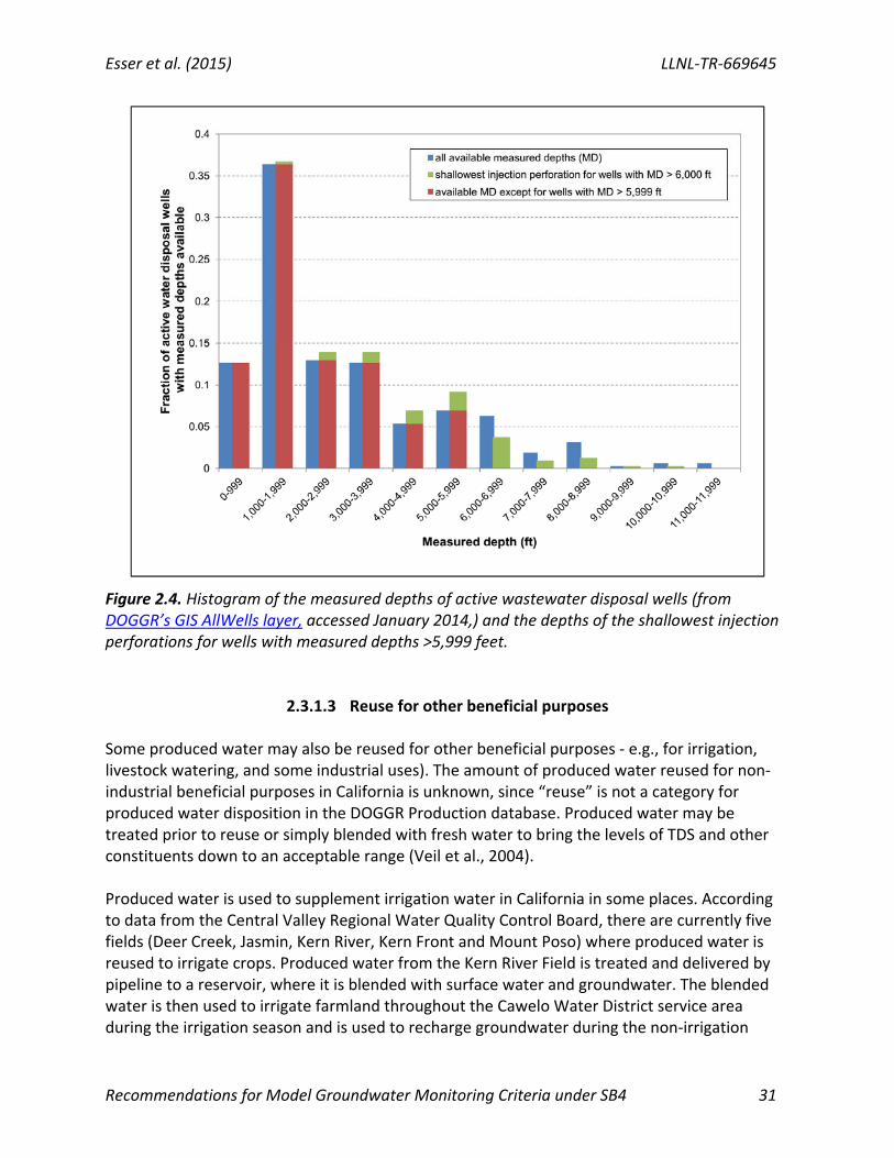
Esser et al. (2015) LLNL‐TR‐669645
Recommendations for Model Groundwater Monitoring Criteria under SB4 31
Figure 2.4. Histogram of the measured depths of active wastewater disposal wells (from DOGGR’s GIS AllWells layer, accessed January 2014,) and the depths of the shallowest injection perforations for wells with measured depths >5,999 feet.
2.3.1.3 Reuse for other beneficial purposes Some produced water may also be reused for other beneficial purposes ‐ e.g., for irrigation, livestock watering, and some industrial uses). The amount of produced water reused for non‐industrial beneficial purposes in California is unknown, since “reuse” is not a category for produced water disposition in the DOGGR Production database. Produced water may be treated prior to reuse or simply blended with fresh water to bring the levels of TDS and other constituents down to an acceptable range (Veil et al., 2004). Produced water is used to supplement irrigation water in California in some places. According to data from the Central Valley Regional Water Quality Control Board, there are currently five fields (Deer Creek, Jasmin, Kern River, Kern Front and Mount Poso) where produced water is reused to irrigate crops. Produced water from the Kern River Field is treated and delivered by pipeline to a reservoir, where it is blended with surface water and groundwater. The blended water is then used to irrigate farmland throughout the Cawelo Water District service area during the irrigation season and is used to recharge groundwater during the non‐irrigation

LLNL‐TR‐669645 Esser et al. (2015)
32 Recommendations for Groundwater Monitoring Criteria under SB4
season (California CVRWQCB, 2012). The Tulare Basin Plan notes that produced water “is used extensively to supplement agricultural irrigation supply in the Kern River sub‐basin” (California CVRWQCB, 2004), and has water quality requirements for the reused water. The use of produced water can potentially provide a new source of water supply, e.g., to farmers in San Joaquin Valley, where water resources are extremely constrained. The use of produced water comingled with flowback fluids, however, raises a set of unique concerns that are not yet well understood, especially when the mixture is not adequately treated prior to reuse. In particular, the toxicity, persistence, and mobility of stimulation chemicals, degradation products and natural constituents mobilized due to stimulation in the flowback/produced water have not yet been evaluated. An evaluation of the treatment technologies, and their capabilities for removing stimulation chemicals and their byproducts is presented in Stringfellow et al. (2015). The typical high levels of TDS and boron in produced water in California pose a limiting factor for the ability to use the produced water for irrigation and careful monitoring of the inorganic constituents in the fresh water‐produced water blend is needed to ensure that the use of produced water is indeed beneficial.
2.3.1.4 Sewer systems Data from the DOGGR production database indicates that a small amount (~1%) of produced waters from oil and gas operations in California are disposed in sanitary sewer systems (Figure 2.3). Between January 2011 and June 2014, most of the discharge into sewer systems occurred in Los Angeles county (106 million barrels or 17 million m3), but some discharge was also reported in Orange county (19 million barrels or 3 million m3) and Kern county (750,000 barrels or 120,000 m3). Operators have to obtain permits prior to discharging into the sewer system, but the pretreatment required is minimal (Stringfellow et al., 2015). In general, sewer systems are not typically equipped to handle high‐salinity produced water (including returned stimulation chemicals), potentially disrupting the treatment process and discharging salt and other contaminants into the environment. Problems with disposal of wastewaters recovered from well stimulation operations into commercial wastewater treatment plants have been noted in some regions. For example, in the early development of the Marcellus region (2008‐2009), flowback and produced waters were legally discharged into public wastewater treatment plants (WWTPs) that were not equipped to handle the high TDS content of these fluids, which resulted in increased loading of salts to Pennsylvania rivers (Kargbo et al., 2010; Vidic et al., 2013; Brantley et al., 2014). Bromide was also found to be a contaminant of concern due to the presence of carcinogenic disinfection byproducts in the WWTPs, formed from the reaction of elevated levels of bromine present in flowback/produced waters with organics (Warner, Christie, et al., 2013; Ferrar et al., 2013; Parker et al., 2014; Harkness et al., 2015). State regulators in Pennsylvania subsequently discouraged the practice

Esser et al. (2015) LLNL‐TR‐669645
Recommendations for Model Groundwater Monitoring Criteria under SB4 33
of discharging waters recovered from fracturing operations into WWTPs, due to the many concerns about water quality degradation. 2.3.2 Potential subsurface leakage pathways The discussion of potential subsurface contamination pathways is organized into four parts. The first part discusses the formation of high permeability pathways by hydraulic fracturing, including the extent and permeability of induced fractures and the possibility of connection to overlying aquifers. The second part addresses issues with active, idle, and abandoned wells that may be pathways for hydrocarbons or fracturing fluids to enter groundwater aquifers. The third part addresses natural features such as faults, fractures and permeable overburden that could lead to transport of potential contaminants into protected groundwater. The last part discusses transport processes that could occur within induced and natural permeable pathways, if they exist, and studies providing evidence of such driving forces. Data concerning these subsurface pathways are limited and the literature on this topic is almost exclusively based on numerical modeling (which is discussed below) without calibration or verification of the modeling.
2.3.2.1 Leakage through hydraulic fractures One possible concern regarding hydraulic fracturing operations is the degree to which induced fractures may extend beyond the target formation to overlying permeable aquifers, or to natural or man‐made pathways such as faults, natural fractures, or abandoned wells. The current state of understanding about the formation of such permeable pathways due to hydraulic fracturing is surrounded by some controversy, due to concerns about groundwater contamination above hydraulically fractured reservoirs. As of 2014, operators in California have been required to submit data on estimated fracture dimensions in well stimulation notices, and actual fracture dimensions in the completion reports. Analysis of the data submitted in 2014 indicate that in about half the operations fractures have been reported to extend up to or shallower than 300 m (1,000 ft) below the ground surface (Stringfellow et al., 2015), which is consistent with a previous finding that the top of the fracturing interval or total depth of the well that was fractured was less than 610 m (2,000 ft) in a majority of the operations (CCST et al., 2014). The analysis also found that the data submitted so far have significant problems with respect to data quality, and that verification of the data was not possible since operators are not required to submit the methods according to which they arrived at these estimates (Stringfellow et al., 2015). For example, all the completion reports indicate only one stage per well, which is inconsistent with data from well records that show the vast majority of operations consist of more than one stage. Thus it is likely that operators are misreporting the number of stages in the well, and that the reported dimensions represent the entire stimulation instead of each individual stage. Furthermore, the reported induced fracture dimensions in a majority of completion reports do not extend above the top of the treatment interval in the well, which seems unlikely. Thus, it is possible that the actual extent of fractures is even shallower than implied the stimulation completion reports.
LLNL‐TR‐669645 Esser et al. (2015)
34 Recommendations for Groundwater Monitoring Criteria under SB4
The vertical extent of induced fractures is especially important to determine because a recent assessment of water quality near oil and gas operations in California, based on the minimum TDS reported in the GAMA database for water supply wells, has found that groundwater with minimum TDS <500 mg/L has been reported in several fields where most of the hydraulic fracturing occurs in California (Stringfellow et al., 2015).The salinity of the water in the oil and gas wells can be much higher, as indicated by geochemical analysis and well logs (Chapter 3, Section 3.3). The vertical separation between protected groundwater with <10,000 mg/L and the top of fracturing intervals still needs to be investigated. The latest and most relevant published work on fracture formation, directly addressing concerns about possible leakage of gas and fracturing fluids, has occurred since 2011. Several recent modeling studies suggest that fracture propagation is inherently limited. Flewelling and Sharma (2014) capped potential vertical fracture propagation at 600 m (2,000 ft) or less and observed that shallow formations are more likely to fracture horizontally rather than vertically. An earlier study found the fracture directionality to have orientations dependent on the unique stress profiles and rock fabric of a given location in addition to depth of the reservoir (Walker et al., 2002). Fisher and Warpinski (2012) compared microseismic data on fracture extent for gas shales, finding that deep hydraulic fracturing operations should not bring the fractures in close contact with shallow aquifers, and that fractures in shallower formations (<1,200 m, or 3,900 ft) have a greater horizontal component. Likewise, Davies et al. (2012) find that the majority of induced fractures (with data focused on the Barnett Shale) range from less than 100 m (330 ft) to about 600 m (2,000 ft) in height, with approximately a 1% probability of a fracture exceeding 350 m (1,100 ft). This leads to a suggested minimum separation of 600 m (2,000 ft) between shale reservoirs and overlying groundwater resources for high‐volume fracturing operations (King, 2012a), although local geology must always be evaluated. Coupled flow‐geomechanical modeling (Kim and Moridis, 2012) also found inherent physical limitations to the extent of fracture propagation—for example, the presence of overlying confining formations may slow or stop fracture growth, thus containing fractures within the shale reservoir (Kim et al., 2014). In California, an industry study (Cardno ENTRIX, 2012) evaluated the effects of ten years of hydraulic fracturing and gas production from a Los Angeles Basin oil and gas field. Microseismic monitoring indicates that fractures were contained within the reservoir zone, extending to within no more than 2,350 m (7,700 ft) of the base of the freshwater (Cardno ENTRIX, 2012). The separation between some fracturing intervals in California and protected groundwater is probably less than the suggested 600 m separation inferred from the modeling studies, which would imply that the likelihood of propagation of fractures into groundwater aquifers may be higher in California. However, it is important to note that this depth‐separation suggestion was based on high‐volume hydraulic fracturing conducted in deep shale reservoirs, meaning the subsurface stress conditions as well as the hydraulic fracturing operations are quite different from the situation in California. For example, due to relatively smaller fracturing fluid volumes, the height distribution of fractures in California may be smaller than that used as the basis for the suggested 600 m depth‐separation. However, the type of hydraulic fracturing implemented in California seeks to focus that fluid into a single fracture propagating from the well in each

Esser et al. (2015) LLNL‐TR‐669645
Recommendations for Model Groundwater Monitoring Criteria under SB4 35
direction, in contrast to type of operation in other parts of the country that seek to create a network of fractures using a larger fluid volume (CCST et al., 2014) (CCST, 2014). Also, the different rock properties of the oil and gas production zones in California requires a careful examination on the magnitude and orientation of fractures propagation following hydraulic fracturing, in particular their close proximity to the overlying shallow aquifers. An important factor for the likelihood of induced fractures entering groundwater is their orientation, which in turn is a function of subsurface stress conditions and hydraulic fracturing operational choices. According to Townend and Zoback (2004), the maximum horizontal compressive stress orientation on the west side of the San Joaquin Valley is fairly uniform and oriented NNE‐SSW, near orthogonal to the San Andreas Fault. Measurements of fractures from shallow horizontal wells in California indicate that they are typically vertical, at least in the southwest San Joaquin Basin, where most shallow fracturing occurs in the state. Emanuele et al. (1998) measured the orientation of fractures resulting from tens of stages in three horizontal wells in the Lost Hills field at a depth of ~600 m (2,000 ft) using surface tiltmeter measurements for each along with subsurface tiltmeter measurements for a few. The orientation of all the fractures was within 10 degrees of vertical. Hejl et al. (2007) reported downhole tiltmeter results in the Lost Hills field indicating vertical to near vertical fracturing at depths as shallow as 425 m (1,400 ft) with NNE‐SSW azimuth exhibiting 5 to 17 degrees standard deviation for multiple induced fractures in the same well. Allan et al. (2010) reported on testing of longitudinal versus transverse fracturing in horizontal wells at a depth of approximately 300 m (1,000 ft) in the South Belridge field. The tests determined wells oriented to create longitudinal fractures were considerably more productive. If fractures propagated horizontally, it would not be possible to create transverse fractures from a horizontal well, and the well orientation would be less relevant to the volume of oil it produced. In addition, Allan et al. (2010) reported that the fractures were vertical, as indicated by surface and downhole tiltmeter measurements. Consequently, there are indications that fracturing at shallow depths in the San Joaquin Basin is predominantly vertical, which means fracturing is more likely to extend upward and encounter protected groundwater. Further investigation is needed to determine the probability that one of these fractures encountering protected groundwater.
2.3.2.2 Leakage through wells (abandoned or active) Oil and gas wells in the vicinity of the stimulated well provide a potential pathway for connections from hydraulic fractures to shallower layers in some locations, and care must be taken to avoid situations where hydraulic fractures intersect other wells. In particular, degraded or improperly plugged abandoned wells, as well as poorly constructed active and idle wells, can serve as contaminant transport pathways. For example, several studies have noted the presence of methane in shallow groundwater near hydraulic fracturing operations, and attribute the likely cause to poor well construction or degraded wells. Sampling studies in drinking water wells in the Marcellus by Osborn et al. (2011) and Jackson et al. (2013) noted that methane concentrations in drinking water wells increased with proximity to gas wells, and that the composition of the sampled gas was similar to the gas from nearby

LLNL‐TR‐669645 Esser et al. (2015)
36 Recommendations for Groundwater Monitoring Criteria under SB4
production wells. Davies (2011) and Schon (2011) suggested that leakage through well casings was a more plausible explanation for the methane than fracturing‐related processes. Further studies (Darrah, Vengosh, et al., 2014; Darrah et al., 2015) found that the gas compositions do not always match the Marcellus gas, suggesting that intermediate formations are in some cases providing the source for the methane, thus indicating that migration occurred through annulus leaking from poorly constructed wells and not from the target reservoir. Based on noble gas geochemistry, Darrah et al. (2014) were able to distinguish between the migration of naturally occurring methane and stray gas contamination from leaking wells. This study identified several locations in the Marcellus in Pennsylvania and the Barnett in Texas where annular migration through or around poorly constructed wells is considered as the most plausible mechanism for measured methane contamination of groundwater. The ability to delineate stray gas contamination in areas where methane is also naturally migrating from deep sources is the key for future monitoring programs and evaluating possible stray gas contamination (Darrah, Vengosh, et al., 2014; Darrah et al., 2015). The hazards of degraded wells and well failure are highlighted in a review paper by Chilingar and Endres (2005). They document multiple incidents in which oilfield gas reached the surface through wells, including some that were abandoned. The paper also highlights a 1985 incident where well casing corrosion at shallow depths led to casing failure of a producing well and the migration of gas via faults and other pathways, leading to gas accumulation in a permeable collecting zone below a populated area in Los Angeles. This zone was beneath a department store, and eventually over‐pressurization drove gas into the building’s basement, resulting in an explosion. While these incidents are not related directly to fracturing operations, they show that cement and casing impairments in modern wells and inadequately cemented abandoned wells may provide pathways for vertical migration of formation gas and fluids. In California, of a total of about 221,000 wells listed in the DOGGR GIS wells file, there are approximately 116,000 wells listed as plugged and abandoned according to state standards, approximately 1,800 older wells that have not been abandoned to standards and approximately 400 wells whose status is unknown (Stringfellow et al., 2015). The accuracy of the locations of the inactive wells listed in DOGGR’s database, and current condition of the abandoned wells is unknown. In addition, the DOGGR idle wells inventory lists, as of December 2014, a total of 21,347 idle wells, although this number differs from the number of idle wells reported in the GIS wells file (13,450 wells). The possibility of operating oil and gas wells (or of water supply wells) serving as leakage pathways for subsurface migration has been known for a long time. Harrison (1983; 1985) indicates that overpressured annuli are a likely mechanism for contamination of groundwater with produced gas or other formation fluids, even for wells using a surface casing to protect shallow aquifers, and particularly if the surface casing does not extend to a sufficient depth below the aquifer. Failures in well barriers (cement and casing strings) may allow intrusion of gas and fluids from producing formations below the casing shoe, or flow from shallower gas and fluid‐bearing formations intersected by the wellbore to lower‐pressure zone above, resulting in annular gas flow or sustained casing pressure (SCP) and a pathway for gas migration

Esser et al. (2015) LLNL‐TR‐669645
Recommendations for Model Groundwater Monitoring Criteria under SB4 37
to overlying aquifers or the surface (Brufatto et al., 2003; Watson and Bachu, 2009). Multiple factors over the operating life of a well may lead to barrier failure including 1) improper or inadequate cementing, 2) poor mud displacement, 3) fractures in the cement due to hydraulic and mechanic stresses during construction or associated with tectonic activity and subsidence events, 4) radial cracking of the cement due to thermal and pressure fluctuations in the casings during stimulation and production, and 5) general degradation of the well structure due to age (Dusseault et al., 2000; Brufatto et al., 2003; Watson and Bachu, 2009; Carey et al., 2013). Corrosive subsurface environments (e.g., H2S, CO2) also pose a threat to cement and casings throughout the life of a well and after abandonment/plugging, particularly if cement is already impaired (Brufatto et al., 2003; Chilingar and Endres, 2005). Even properly cemented wells may develop leaks over time because of cement deterioration in the high salinity fluids (Ingraffea et al., 2014). The long term deterioration of cement has been little studied and needs further research. However, the most important mechanism leading to gas and fluid migration, is poor well construction or exposed or uncemented casing (Watson and Bachu, 2009). Unconventional wells may be subject to greater stresses due to mechanical stresses induced in high pressure stimulation and lateral drilling practices used to create deviated well bores (Ingraffea et al., 2014). Watson and Bachu (2009) also noted that deviated wellbores, defined as “any well with total depth greater than true vertical depth”, have a higher frequency of sustained casing pressure and gas migration than vertical wells, likely due to centralization and cementing challenges increasing the likelihood of gaps, bonding problems, or thin regions in the cement. Creation of such annular permeable pathways may create connectivity to shallower formations. During hydraulic fracturing operations, there has been concern that the expansion and contraction of the steel casing during the multiple stages of high‐pressure injection may result in radial fracture and/or shear failure at the steel‐concrete or concrete‐rock interfaces (Carey et al., 2013). These processes could create gaps or channels that would serve as conduits between the various strata through which the well penetrates. For some operations, though, the fracturing fluid is pumped down a tubing string within the innermost casing, such that the casing and surrounding cement do not experience the high injection pressure associated with the fracturing operation. However, less complex stimulation treatments, such as some, and perhaps most, California operations, may instead inject the fracturing fluids through the production casing, which would expose the casing and seal beyond to mechanical stresses caused by the injection pressure. In a review of the regulatory record, Vidic et al. (2013) noted a 3.4% rate of cement and casing problems in Pennsylvania wells based on filed notices of violation. Pennsylvania inspection records, however, show a large number of wells with indications of cement/casing impairments for which violations were never noted suggesting the actual rate of occurrence could be higher than that reported by Vidic et al. (2013). In addition, several mechanisms such as surface subsidence, reservoir compaction or heaving, or even earthquakes can lead to well impairment due to casing shear (Dusseault et al., 2001).

LLNL‐TR‐669645 Esser et al. (2015)
38 Recommendations for Groundwater Monitoring Criteria under SB4
The diatomite formations in Kern County are highly porous and compressible, and hence are particularly susceptible to depletion‐induced compaction. For example, several wells failed in the 1980s in Belridge (at a peak rate of 160 wells per year) following years of active production enabled by stimulation, which led to reservoir depletion and subsidence (Fredrich et al., 1996; Dusseault et al., 2001) Waterflood programs were then initiated to counter the subsidence, which led to much lower rates of well failure in the late 1990s of around 2‐5% of active wells per year or approximately 20 wells per year (De Rouffignac et al., 1995; Fredrich et al., 1996; Dusseault et al., 2001). The current situation with groundwater overdraft in the southern San Joaquin valley may pose an added risk to wells in the region due to subsidence. Earthquakes can also lead to casing shear; for example hundreds of oil well casings were sheared in the Wilmington oil field in Los Angeles during five or six earthquakes of relatively low magnitude (M2 to M4) during a period of maximum subsidence in the 1950s (Dusseault et al., 2001). Human error during the well‐completion and hydraulic fracturing process must also be considered. A 2011 incident in Alberta, Canada involved inadvertent fracturing of an overlying formation and injection of fluids into water‐bearing strata below an aquifer (Energy Resources Conservation Board, ERCB, 2012). Misreading of well fluid pressures resulted in the perforation gun being fired at 136 m depth (446 ft) rather than the specified 1,486 m (4,875 ft), with subsequent pressurization creating a fractured interval above the base of protected groundwater. Immediate flowback of fracturing fluids recovered most of the injected volume, and monitoring wells were installed at the perforation depth and at 81 m (266 ft) in an overlying sandstone aquifer at a distance of 50 m (164 ft). A hydraulic connection between the fractured interval and the overlying aquifer was not observed, and a surface gas release nearby was not linked to the injected fluids. The ERCB finding states that the incident presented “insignificant” risk to drinking water resources, but criticized the onsite crew’s risk management, noting there were multiple opportunities to recognize abnormal well behavior before injection of fluids. Well integrity must also be evaluated for Class II deep injection wells, which have become the method of choice for the disposal of produced water. The longer injection duration and larger injection volume used in Class II injection wells increases the probability of compromised well integrity (Yuan et al., 2013). In California, a 2011 report studied the over‐24,000 active and 6,900 inactive injection wells in the state and found that, while procedures were in place to protect fresh‐water resources, other water resources (with higher levels of dissolved components, but still requiring protection as Underground Sources of Drinking Water (USDW)) may be at risk due to deficiencies in required well‐construction practices (USEPA, 2011b).The report also states that “zonal isolation of saline aquifers from USDWs by cement placement is not required and isolation from hydrocarbon bearing zones open to the uncemented wellbore is not assured without cement placement at the base of USDWs. That leaves those USDWs exposed to fluid movement due to Improperly plugged wells and/or lack of cement in the casing/wellbore annulus, notwithstanding the presence of drilling mud that may restrict fluid flow” (Walker, 2011). In addition, depending on the target formation, injection pressures must be monitored and maintained at or below levels appropriate for the geology. In addition, operators are required to perform mechanical integrity tests on Class II wells every five years.

Esser et al. (2015) LLNL‐TR‐669645
Recommendations for Model Groundwater Monitoring Criteria under SB4 39
A US Government Accountability Office report (USGAO, 1989) regarding Class II wells across the United States documented several cases of contamination of drinking water that were detected from 1970 to 1988. In one‐third of the cases, the contamination was caused by communication between injection wells and improperly plugged (abandoned) oil and gas wells nearby, causing injected brines to migrate vertically through the abandoned wellbores. Injection wells built and operating prior to 1976 are exempt from Underground Injection Control (UIC) program permitting requirements (40 CFR 144.31, 146.24), which mandate an area search for abandoned wells within the Area of Review around the proposed injection well. The GAO report notes that 70% of the injection wells studied were constructed and began operation prior to UIC requirements, and as such the presence of nearby degraded wells was discovered only after contamination had occurred. A recent follow‐up report (USGAO, 2014) recommended that EPA review emerging risks related to class II program safeguards and ensure that it can effectively oversee and efficiently enforce class II programs. The GAO also concluded that EPA should take actions to ensure it can enforce state class II regulations, as discussed in the report (USGAO, 2014) 2.3.2.3 Leakage through natural fractures, faults and other natural subsurface features
Several modeling studies have attempted to elucidate mechanisms of subsurface transport in fractured formations through numerical simulation, and are described in Stringfellow et al. (2015). Sampling and field studies have also sought evidence of migration, but the bulk of the peer‐reviewed work focuses on the Marcellus Shale, and no such studies have been conducted in California. A key conclusion from these studies is that pathways and mechanisms are difficult to characterize and the role of fracturing or transport through fractures has not been clearly established. Fault activation resulting in the formation of fluid pathways is an additional concern when stimulation operations occur in faulted geologies, such as in California (Stringfellow et al., 2015). Fault activation is a remote possibility for faults that can admit stimulation fluids during injection (Rutqvist et al., 2013)possibly increasing the permeability of previously sealed faults or creating new subsurface pathways analogous to induced fractures (possibly on a larger scale). Chilingar and Endres (2005) document a California incident, where the migration of gas via permeable faults (among other pathways) created a gas pocket below a populated area in Los Angeles and resulted in an explosion. While the incident was not related to stimulation operations, it shows how naturally faulted geologies can provide pathways for migration of gas and fluids. 2.3.2.4 Driving forces: Mechanisms of leakage via transport through subsurface pathways Although mechanisms for transport through fractures and faults have been proposed, few conclusions can yet be made about the conditions under which liquid or gas release can occur. Overburden thickness, formation permeabilities, production strategies (assuming no drilling or casing incidents), and other site‐specific factors may all regulate the probability of contaminant

LLNL‐TR‐669645 Esser et al. (2015)
40 Recommendations for Groundwater Monitoring Criteria under SB4
migration. A recent study by Kissinger et al. (2013) consisted of porous‐media modeling of liquid and gas migration through specific, previously characterized fractured systems. The study, although limited to one set of geological models (and thus to one set of subsurface geometries), does highlight factors that may increase or decrease the risk of contamination. Fluid migration resulting from a two‐week fracturing‐related overpressure is shown to drive fracturing fluids only a limited distance from the fractured reservoir, even when high‐permeability pathways are assumed. Long‐term tracer transport and transport of methane to overlying aquifers are shown to be a function of pathway porosity, permeability, and irreducible gas saturation, but only under the assumption of a continuous permeable pathway from the reservoir to the aquifer. Factors such as production strategy or ranges of overburden thickness are not evaluated, but Kissinger et al. (2013) suggest that transport of liquids, fracturing fluids, or gas is not an inevitable outcome of fracturing into connected pathways, and that further evaluation of a range of geological systems is warranted. Also liquid and gas transport do not necessarily occur together, and may occur at different rates and times. Geochemical evidence for natural migration of brines has been published by Warner et al. (2012a). The study indicated that elevated salinity levels in the region may predate shale gas production in the area, and that geochemical signatures matching that of the Marcellus fluids led to the conclusion that naturally permeable pathways may have already existed between the shale and overlying formations through geologic time. The possibility that naturally permeable pathways could create contamination hazards if oil and gas operations occur near the zones of enhanced connectivity was disputed by Engelder (2012), who notes that recent drilling data for hundreds of wells suggests the saturation of water in the pore space of the types of rocks targeted for fracturing is typically in the range of 13% to 33%, which is near or below the irreducible water saturation for the shale. Such low saturations would result in capillary binding of the water, restriction of brine migration, and the possible sequestration of fracturing fluids left in the formation, as the aqueous phase would be drawn into the pore space of the shale and rendered immobile. This capillary seal would be expected to trap both gas and liquids within the Marcellus, and this concept is supported by differences in the isotopic signature of Marcellus gas and gas that exists in the overlying formations (see also Molofsky et al., 2013a). The work by Flewelling et al. (2013) also addresses this issue of formation isolation, pointing out that the occurrence of permeable pathways overlying significant hydrocarbon accumulations is inherently contradictory. Therefore, their work finds that some mechanism that activates pre‐existing, but impermeable features or creates new pathways is necessary to allow liquid and gas migration, while noting the potential constraints to vertical fracture propagation mentioned in the previous section. A further response by Warner et al. (2012b) maintains that there are insufficient data to support the capillary binding hypothesis, and that recent production data counter the notion that the shale has little mobile brine—in fact, the opposite has been true for some production wells—but also concedes that mechanisms for rapid brine transport are neither indicated nor understood. These studies are likely not relevant to most hydraulic fracturing operations in California, which occur at shallower depths and more permeable rock. Water production from these wells is continuous, rather than tapering off with time as in most wells hydraulically fractured in other parts of the country.
Esser et al. (2015) LLNL‐TR‐669645
Recommendations for Model Groundwater Monitoring Criteria under SB4 41
While the debate on migration of deep brine has focused on water transport within the shale formation, geological formations overlying the shale formation with high permeability could also host formation water that could be mobilized to shallow aquifers upon changes in hydrological conditions. Attempts to perform mathematical risk assessments of contamination through all mechanisms have primarily highlighted the lack of knowledge (Rozell and Reaven, 2012) with envelopes of uncertainty spanning orders of magnitude. Although when risk is formally assessed, the consequences of wastewater disposal (i.e., potentially large spills) generate more concern than subsurface leakage and migration. Further field and modeling studies are needed to elucidate possible transport mechanisms. In this regard, additional studies are under way to identify tracer materials that could be useful for the monitoring of the migration of fracturing fluids in the subsurface, as well as fracturing fluid‐shale interactions. For instance, nanoparticles, which could be added as nonreactive tracers to fracturing fluids in the future, are currently being tested (Maguire‐Boyle and Barron, 2014). The analysis of strontium (Sr) isotope ratios has been proposed as a useful approach to evaluate fluid‐rock interactions (Chapman et al., 2012). Boron and lithium isotopes have been shown to have distinctive isotope ratios in flowback waters from hydraulic fracturing that are different from the boron and lithium isotope compositions in conventional oil and gas produced water (Warner et al., 2014). In either case, these tracers could provide relevant tools for elucidating open questions regarding potential contaminant pathways related to well stimulation applications in the future.
2.3.3 Surface spills and leaks Spills and leaks of additives used during operations or of flowback/produced water can potentially contaminate water resources due to run off into surface water bodies and/or seepage into groundwater aquifers. Surface spills and leaks can occur during chemical or fluid transport, pre‐stimulation mixing, during stimulation, and during wastewater handling after stimulation. In addition, onsite pits or containers used for storage or chemicals and wastewater can leak. Spills or leaks can also result from tank ruptures, piping failures, blowouts, equipment failures and defects, overfills, fires, vandalism, accidents, or improper operations (NYDEC, 2011)). For example, in September 2009, two pipe failures and a hose rupture in Pennsylvania released 8,000 gallons of a liquid gel mixture during the hydraulic fracturing process, polluting a local creek and wetland (Pennsylvania DEP, 2009b; Pennsylvania DEP, 2009a). Data on hazardous materials spills are maintained by the California Emergency Management Agency (CEMA). According to California law, any significant release or threatened release of hazardous substances must be reported to CEMA. Data on flowback/produced water spills associated with oil and gas operations in California are reported to the DOGGR. According to the California Code of Regulations Title 14 Section 1722, “significant” water leaks must be promptly reported to the appropriate DOGGR district office. The reporting requirements are vague. There is no definition of what constitutes a significant leak, and all spills are likely not reported.

LLNL‐TR‐669645 Esser et al. (2015)
42 Recommendations for Groundwater Monitoring Criteria under SB4
According to the available data, nearly 2.8 million gallons of flowback/produced water were released in 423 surface spills at oil and gas fields in California between January 2009 and February 2014, which is on average 6,500 gallons per incident (CCST et al., 2014). Corrosion and sensor failures that cause tanks to overflow are listed as the most common causes of these spills. Further analysis of spills data are presented in Stringfellow et al. (2014). Spills of chemicals typically used in well stimulation fluids, e.g., hydrochloric, hydrofluoric, and sulfuric acids, have also occurred at oil and gas operations in California. For example, in February 2012, a storage tank containing 5,500 gallons of hydrochloric acid exploded in the Midway‐Sunset Oil Field in Kern County, spreading the acid beyond a secondary containment wall. It is not possible, however, to discern whether stimulation was the intended purpose of this chemical, because acids are also used to dissolve drilling mud that has invaded the reservoir before the well is brought into production, and minerals that precipitate in the well over time during production, and so are not uniquely associated with well stimulation. Surface spills have the potential to intercept groundwater aquifers, although the lack of data on underlying groundwater quality before and after spills, lack of data on the chemical composition of the spills, and varying conditions across the state limit the ability to evaluate general potential impacts to groundwater in California. There is evidence from other states that surface spills of flowback/produced water can affect surface water bodies and groundwater aquifers. For example, in 2007, flowback fluids overflowed retention pits in Knox County, KY, releasing the fluid directly into Acorn Fork, killing, harming or displacing all fish, invertebrates, and other biota for months over a 2.7 km (1.7 miles) section of the creek (Papoulias and Velasco, 2013). In another analysis of surface spills between July 2010 and July 2011 in Weld County, CO, Gross et al. (2013) found that surface spills of produced water from the fracturing process or crude oil from fractured wells released BTEX to groundwater at levels that exceeded National Primary Drinking Water Maximum Contaminant Levels (MCLs) for each compound. In general, remediation efforts were sufficient to address these spills.

Esser et al. (2015) LLNL‐TR‐669645
Recommendations for Model Groundwater Monitoring Criteria under SB4 43
3 PROTECTEDGROUNDWATERINCALIFORNIA
3.1 Definitions®ulatoryframework In a typical basin, the salinity of groundwater increases with increasing depth in the subsurface (Figure 3.1). Deep groundwater salinity may be the result of a number of causes:
In marine sediments, a large percentage of the original seawater (often termed connate water) may have been trapped within the pore spaces after deposition.
In deep layers with little atmospheric contact and flushing by fresher meteoric waters, water‐rock interactions, including the dissolution of the aquifer minerals and other chemical reactions may increase the salinity of the pore fluids over time.
These chemical processes are amplified by the higher temperatures which normally exist at greater depths. The US EPA’s Underground Injection Control (UIC) Program is responsible for regulating the construction, operation, permitting, and closure of injection wells that place fluids underground for storage or disposal (http://water.epa.gov/type/groundwater/uic/index.cfm, accessed 12/29/2014). The UIC permitting process requires a listing of all Underground Sources of Drinking Water (USDW) that may be affected by injection operations (Figure 2.1). This may require evaluation of formations extending some distance from the site, especially in areas where pressures may be affected by injection activities for a significant lateral area from the injection well. This list must include the geologic name and the depth to the base of all USDWs that may be affected. The California Oil and Gas Well Stimulation Bill (SB4) passed on September 20, 2013. This bill amdended the California Public Resources Code and Water Code to require groundwater monitoring of well stimulation operations in the state. In order to define the scope of monitoring programs, an operational definition of groundwater requiring protection is needed. California protects beneficial use of water under the provisions of the Porter‐Cologne Water Quality Control Act. In general, all waters are considered to have potential for beneficial use unless exempted from such a designation. Under California SWRCB Resolution No. 88‐63 (1988), groundwaters are considered suitable as a source of municipal or domestic water supply (a beneficial use abbreviated as MUN) with the exception of waters where
The total dissolved solids (TDS) exceed 3,000 mg/L (5,000 uS/cm, electrical conductivity) and it is not reasonably expected by Regional Boards to supply a public water system, or
LLNL‐TR‐669645 Esser et al. (2015)
44 Recommendations for Groundwater Monitoring Criteria under SB4
There is contamination, either by natural processes or by human activity (unrelated to the specific pollution incident), that cannot reasonably be treated for domestic use using either Best Management Practices or best economically achievable treatment practices, or
The water source does not provide sufficient water to supply a single well capable of producing an average, sustained yield of 200 gallons per day, or
The aquifer is regulated as a geothermal energy producing source or has been exempted administratively pursuant to 40 Code of Federal Regulations, section 146.4 for the purpose of underground injection of fluids associated with the production of hydrocarbon or geothermal energy, provided that these fluids do not constitute a hazardous waste under 40 CFR, section 261.3.
The depth to which groundwaters containing less than 3,000 mg/L TDS extend is commonly referred to as the Base of Fresh Water (BFW). Other definitions of fresh water are in the literature and in regulation. Page (1973) defines fresh water as “water having a maximum specific conductance of 3,000 micromhos per centimeter, about 2,000 mg/l dissolved solids”. His rationale was that 3,000 micromhos/cm had been used for mapping the base of fresh water in the Sacramento Valley, and the Federal Water Pollution Control Administration considered 2000 mg/l to be a limiting dissolved solids content for the irrigation of most crops. California sets a Secondary Maximum Contaminant Level (SCML) for TDS in drinking water of 500 mg/L with an upper limit of 1,000 mg/L and a short‐term upper limit of 1,500 mg/L (Table 3.1). In this document we will refer to Fresh Water as water having less than 3,000 mg/L TDS and considered by the State to have the potential for beneficial use as a domestic or municipal water supply. Regional Boards have discretion to define exemption criteria for other beneficial uses of water. In the Tulare Lake Basin, in which most well stimulation in California occurs, The Central Valley RWQCB considers all of the above criteria with the exception of salinity in making exceptions to the beneficial use designation of agricultural supply (AGR) (California CVRWQCB, 2004). In making exceptions to the beneficial use designation of industrial supply (IND or PRO), the Central Valley RWQCB considers only pollution status and yield and does not consider salinity or energy production. Federal laws target the protection of groundwater resources for drinking water supplies and define these as resources containing less than 10,000 mg/l TDS (commonly referred to as Underground Sources of Drinking Water or USDW). The USEPA defines a USDW as “An aquifer or portion of an aquifer that supplies any public water system or that contains a sufficient quantity of ground water to supply a public water system, and currently supplies drinking water for human consumption, or that contains fewer than 10,000 mg/l total dissolved solids and is not an exempted aquifer.” (40 CFR § 146.3). This definition includes aquifers (and portions of aquifers) that do not currently supply water to a public water supply but are capable of producing that water.
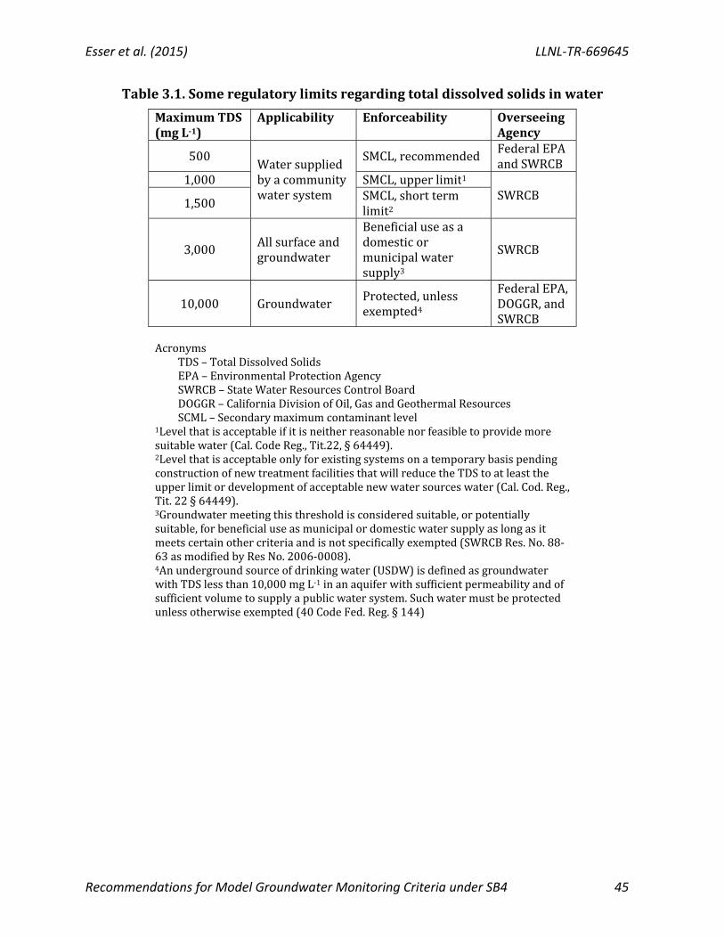
Esser et al. (2015) LLNL‐TR‐669645
Recommendations for Model Groundwater Monitoring Criteria under SB4 45
Table3.1.Someregulatorylimitsregardingtotaldissolvedsolidsinwater
MaximumTDS(mgL‐1)
Applicability Enforceability OverseeingAgency
500Watersuppliedbyacommunitywatersystem
SMCL,recommended FederalEPAandSWRCB
1,000 SMCL,upperlimit1SWRCB
1,500SMCL,shorttermlimit2
3,000 Allsurfaceandgroundwater
Beneficialuseasadomesticormunicipalwatersupply3
SWRCB
10,000 GroundwaterProtected,unlessexempted4
FederalEPA,DOGGR,andSWRCB
Acronyms
TDS–TotalDissolvedSolidsEPA–EnvironmentalProtectionAgencySWRCB–StateWaterResourcesControlBoardDOGGR–CaliforniaDivisionofOil,GasandGeothermalResourcesSCML–Secondarymaximumcontaminantlevel
1Levelthatisacceptableifitisneitherreasonablenorfeasibletoprovidemoresuitablewater(Cal.CodeReg.,Tit.22,§64449).2LevelthatisacceptableonlyforexistingsystemsonatemporarybasispendingconstructionofnewtreatmentfacilitiesthatwillreducetheTDStoatleasttheupperlimitordevelopmentofacceptablenewwatersourceswater(Cal.Cod.Reg.,Tit.22§64449).3Groundwatermeetingthisthresholdis consideredsuitable,orpotentiallysuitable,forbeneficialuseasmunicipalordomesticwatersupplyaslongasitmeetscertainothercriteriaandisnotspecificallyexempted(SWRCBRes.No.88‐63asmodifiedbyResNo.2006‐0008).4Anundergroundsourceofdrinkingwater(USDW)isdefinedasgroundwaterwithTDSlessthan10,000mgL‐1inanaquiferwithsufficientpermeabilityandofsufficientvolumetosupplyapublicwatersystem.Suchwatermustbeprotectedunlessotherwiseexempted(40CodeFed.Reg.§144)

LLNL‐TR‐669645 Esser et al. (2015)
46 Recommendations for Groundwater Monitoring Criteria under SB4
Figure 3.1. Salinity typically increases with depth in underground aquifers (USEPA, 2002). The State of California considers waters with less than 3,000 mg/L TDS as suitable or potentially suitable for the beneficial use of municipal or domestic water supply. Graphics by Sascha Madrid. An aquifer that meets the criteria for a USDW can be exempted from such a designation if it meets certain criteria. The designation of “exempted aquifer” allows for industrial waste, oil and gas, and mine related injection through the Underground Injection Control Program. Regulation 40 CFR § 146.4 requires certain criteria be met for an aquifer to be designated an “exempted aquifer”.
(a) The aquifer does not currently serve as a source of drinking water; and

Esser et al. (2015) LLNL‐TR‐669645
Recommendations for Model Groundwater Monitoring Criteria under SB4 47
(b) The aquifer cannot now and will not in the future serve as a source of drinking water because:
a. It is mineral, hydrocarbon or geothermal energy producing, or can be demonstrated by a permit applicant as part of a permit application for a Class II or III operation to contain minerals or hydrocarbons that considering their quantity and location are expected to be commercially producible.
b. It is situated at a depth or location, which makes recovery of water for drinking water purposes economically or technologically impractical;
c. It is so contaminated that it would be economically or technologically impractical to render that water fit for human consumption; or
d. It is located over a Class III well mining area subject to subsidence or catastrophic collapse; or
(c) The total dissolved solids content of the ground water is more than 3,000 and less than 10,000 mg/l and it is not reasonably expected to supply a public water system.
A fourth criterion extends the exemption from Class II wells used for enhanced oil recovery to Class VI wells for geologic storage of carbon dioxide. At issue for California is that the depths, salinities, and levels of contamination that render the beneficial use of water economically impractical will change under drought conditions and over time. Future demands for beneficial groundwater use are likely to grow in California as fresh water sources are diminished under drought conditions and treatment technologies will improve over time and become more economic. Under Porter‐Cologne, all groundwaters are protected from degradation unless specifically exempted. We recommend monitoring groundwaters containing up to 10,000 mg/L TDS, and when we refer to “protected groundwater”, we are referring to water with up to 10,000 mg/L TDS that is not exempt from groundwater monitoring. Choosing 10,000 mg/L as an upper limit of salinity for groundwaters to be monitored aligns WST groundwater monitoring with the federal definition of USDW and the Class II Underground Injection Control program (which is operative in several of the oil and gas fields and pools being stimulated). The choice of 10,000 mg/L also provides a useful target for assessment of and recommendation to improve the state of knowledge on the distribution of groundwater of various salinities in the State. In our recommendations, we will also distinguish between groundwaters containing less than 3,000 mg/L and groundwaters with between 3,000 and 10,000 mg/L, and recommend that groundwater containing less than 3,000 mg/ be monitored more intensively. 3.2 Currentstateofknowledgeofthedistributionof0‐3,000mg/Land
3,000‐10,000mg/LgroundwaterinCalifornia Information regarding the groundwater quality of California aquifers is available from a number of state and federal agencies. One source is the California and Nevada chapter of the Ground Water Atlas of the United States published by the US Geological Survey (Planert and Williams, 1995) (http://pubs.usgs.gov/ha/ha730/ch_b/index.html, accessed March 27, 2015). The atlas

LLNL‐TR‐669645 Esser et al. (2015)
48 Recommendations for Groundwater Monitoring Criteria under SB4
divides California into five major aquifer systems: the basin and range aquifers, the Central Valley aquifer, the coastal basins aquifers, the northern California basin fill aquifers and the northern California volcanic rock aquifers. The thickness of the aquifers containing waters with less than 1,000 mg/L TDS are mapped. The report also provides maps of areas with known water quality issues including seawater intrusion, selenium and pesticide impacts. Currently, there is no database or detailed map delineating the lateral and vertical extent and location of the aquifers containing waters with less than 3,000 and 10,000 mg/L TDS, although an effort is underway to fill this data gap (see Section below).
Water well chemical analysis data are available from monitoring wells operated by the USGS and the California State Board of Water Resources:
1) US Geological Survey (USGS) http://nwis.waterdata.usgs.gov/ca/nwis/qwdata, accessed 12/20/2014
2) California State Water Resources Control Board (SWRCB) http://geotracker.waterboards.ca.gov/, accessed 12/29/2014
These sites contain a variety of data including TDS values, approximate location, well depth and the concentration of various analytes. Not all of these data were available at a particular site, especially data regarding well completion intervals. Well completion data are available from the California Department of Water Resources (DWR) however state laws limits the disclosure of this information making it very difficult for the general public, private entities or even federal agencies or state universities to determine the depths at which waters of various salinities are found. There are other publications that deal with specific areas of California. In the case of the San Joaquin Valley in California, Page (1973) has constructed maps to the base of fresh water (2000 mg/l TDS). County agencies such as the Kern County Water Agency (KCWA) also publish annual maps of depth to groundwater and groundwater quality in Kern County (http://www.kcwa.com/, accessed 3/27/2015). The above sources of information are usually oriented to drinking water aquifers of low TDS content and the salinity is almost always less than 3000 mg/L, thus they are of limited assistance in locating the depth to deeper, more saline aquifers. DOGGR maintains a website containing scanned copies of chemical analyses of oilfield waters taken at various depths (ftp://ftp.consrv.ca.gov/pub/oil/D4%20Chemical%20Analysis/, accessed 12/30/2014). This database is invaluable in determining the water quality and extent of the deeper, more saline aquifers necessary to determine the 3000 mg/L and 10,000 mg/L boundaries in the subsurface. While direct sampling and chemical analyses found in the databases above are the best method for determination of TDS in any aquifer, in many cases (particularly in deep aquifers) these analyses are uncommon. However, in active petroleum‐producing basins, open‐hole geophysical logs are available in abundance. Of particular interest for determining water salinity
Esser et al. (2015) LLNL‐TR‐669645
Recommendations for Model Groundwater Monitoring Criteria under SB4 49
are the electrical logs (spontaneous potential (SP) and resistivity) because the ability of water to conduct an electrical current is determined by both the temperature and salinity of the formation water. The US EPA (2002; http://water.epa.gov/learn/training/dwatraining/upload/dwaUIC‐uicpermit.pdf, accessed 12/29/2014) discusses two different methods of determining salinity from geophysical logs. One of the methods for determining water salinity from open‐hole logs is the resistivity‐porosity (RP) method and requires data from a deep resistivity log and a porosity log (or core data). The other method is the Spontaneous Potential method (SP) and uses only the SP curve from the electric log. These methods are discussed in detail by Jorgensen (1989) and US EPA (2002). Neither method provides specific ion concentrations but either can be used to estimate salinity values.
3.3 CurrentEffortstoMapGroundwaterSalinityintheSanJoaquinValley
The southern San Joaquin Valley (SJV) in Kern County is the largest petroleum‐producing area in the state of California. The increased use of hydraulic fracturing in many parts of the country has raised concerns about its potential impacts on water quality in the petroleum‐producing areas of California. The largest number of permits for well stimulation via hydrofracture are issued for operations in the San Joaquin Valley. Page (1973) defined fresh water as water with less than 2000 mg/l TDS because it was a limiting dissolved solids content for the irrigation of most crops. Page (1973) used a resistivity log cutoff
of 3,000 mhos/cm to define the base of fresh water in the SJV. His maps of the base of fresh water (BFW) are currently used by most state officials to determine the location of groundwater which must be protected. In order to comply with the more stringent definition of USDW’s as defined by the US EPA, it is necessary to have accurate information regarding the location and depth of USDW’s within the basin. However, the base to the USDW has not been determined in the southern San Joaquin Valley making it difficult to know where the US EPA regulations are applicable. Analyses of water from wells used for various oil and gas production activities are available online for DOGGR District 4 (ftp://ftp.consrv.ca.gov/pub/oil/D4%20Chemical%20Analysis/, accessed 12/30/2014). Dr. Jan Gillespie at California State University, Bakersfield subjected the analyses for wells in the Kern County area to various quality control methods including charge balance for the analytes sampled and a comparison of the date of chemical testing to the date of initial production from or injection into the well. The most accurate samples come from zones that have produced several well volumes and have not yet experienced injection for wastewater disposal or EOR. The sampled wells were incorporated into a GIS database where the salinity and the depth of the sampled interval could be examined visually (Figures 3.2 and 3.3). In areas with numerous analyses, outliers (i.e. wells markedly more fresh or saline

LLNL‐TR‐669645 Esser et al. (2015)
50 Recommendations for Groundwater Monitoring Criteria under SB4
compared to nearby wells sampled at similar depth) were removed from the GIS database and highlighted as potential erroneous data points in the main database.
Figure 3.2. Map of western Kern County showing wells with geochemical analyses color coded to display the salinity of their formation waters. Dark blue wells have waters with less than 3000 ppm and light blue wells have salinities ranging from 3000 to 10,000 ppm. These waters are considered protected by US EPA guidelines if they are outside exempt aquifers. The resulting GIS map shows that most of the fresh water occurring in wells related to oil and gas production in the SJV is on the east side of the valley and continues as far west as the metropolitan core of Bakersfield. East of Bakersfield, USDW waters are commonly found all the way to basement. The greatest depth to USDW was found in the Mountain View oilfield where one sample tested 6675 ppm in the Chanac Formation at a depth of 6600 feet. West of Bakersfield, the orange and red dots indicate salinities near that of seawater, however most of these wells tap much deeper aquifers. Fresh water is still present in the shallow subsurface. The Tulare Formation is the zone most likely to contain waters classified as USDW, however the Potter sands at north Midway‐Sunset field also often contains USDW’s at depths of up to 1700 feet.

Esser et al. (2015) LLNL‐TR‐669645
Recommendations for Model Groundwater Monitoring Criteria under SB4 51
Figure 3.3. Three dimensional map of aquifer salinity shows the depths to the sampled intervals in oil and gas wells in the Kern County portion of the San Joaquin Valley. Oil fields are shown in tan, city limits in green, major highways in black. Log analysis was used to estimate the depth to the base of USDW’s in areas both with and without geochemical analyses. It is especially useful in those areas without samples near the base of USDW. Electric logs for most of the wells in DOGGR District 4 of the SJV are available from DOGGR (http://www.conservation.ca.gov/dog/Pages/Wellfinder.aspx, accessed 4/20/15). The resistivity‐porosity (RP) method provided consistently better results than the spontaneous potential (SP) method. Therefore, the RP method was used to estimate the depth to the base of USDW’s in various wells throughout the Kern County portion of the San Joaquin Valley (Figure 3.4). The estimated depths from log analysis were then compared to the chemical analysis data. A contour map to the base of USDW estimated from log analysis is shown in Figure 3.4. The RP method worked well in general. It predicts the depth to USDW with reasonable accuracy as noted by the chemical analyses in the majority of the area analyzed. Areas not analyzed include the eastern and westernmost margins of the basin. Along the eastern margin of the field in the Round Mountain, Mount Poso and eastern Edison fields, USDW’s persist to basement depths except for the Olcese sands. The base of USDW in part of this area often occurs within the thick shale zones of the Round Mountain and Freeman silts. In these areas, it was impossible to pick a precise depth for the base of USDW. On the west side of the valley (along and west of Highway 33) USDW (where present) occur within the oil sands and cannot be defined by standard log analysis methods. In the

LLNL‐TR‐669645 Esser et al. (2015)
52 Recommendations for Groundwater Monitoring Criteria under SB4
southernmost part of the basin near Tejon embayment, high resistivity sands persist at depths as great as 10,000 feet in some wells, however chemical analyses at Wheeler Ridge in this area indicate that the USDW only exist above approximately 3500 feet (Figure 3.5). The reason for this discrepancy is unclear however, there are few chemical analyses in this area and it is apparent that more analyses will be vitally important in determining the depth to the base of USDW in the southernmost part of the basin as well as along the far western margin.
Figure 3.4. Contour map (C.I. = 500 feet) to the base of USDW (10,000 ppm) estimated from log analysis by California State University, Bakersfield. Values are in measured depth below surface elevation. Only the area between the red dashed lines were used in the analysis. Wells to the east of the area have USDW to basement or within a thick shale zone. Wells to the west have USDW’s (where present) occurring within the oil zone. Log analysis incorrectly estimated the depth to the base of USDW in the southernmost part of the basin.

Esser et al. (2015) LLNL‐TR‐669645
Recommendations for Model Groundwater Monitoring Criteria under SB4 53
Figure 3.5. Three dimensional surface map of the base of USDW (10,000 ppm) estimated from log analysis. The values are in measured depth below log elevation (usually in reference to a Kelly Bushing 10 to 20 feet above ground surface) and are shown as negative values. Darker shades indicate deeper depths to the base of USDW. Only the area between the red dashed lines were used in the analysis. Depth to top of the perforated interval in wells with chemical analyses is also shown. A comparison of the chemical analysis results to the salinity estimated from log analysis show that the log analysis works well within the area between the red dashed lines except for the southernmost end of the valley. In this area, the logs give a deeper estimate of the base to USDW than indicated by the available chemical analyses.
Note: A more complete description of this study is included the appendix “Current Efforts to Map Groundwater Salinity in San Joaquin Valley” by Dr. Jan Gillespie.
LLNL‐TR‐669645 Esser et al. (2015)
54 Recommendations for Groundwater Monitoring Criteria under SB4
4 MONITORINGTHEIMPACTOFOILANDGASDEVELOPMENTONGROUNDWATER
4.1 MonitoringoutsideofCalifornia States use different approaches for monitoring drinking‐water aquifers near oil and gas wells. Their approaches range from no required baseline testing of water quality, mandatory pre‐ and post‐drilling testing of water quality, and a rebuttable presumption of liability to a specified distance from the oil or gas well. Texas, Louisiana, and Oklahoma for example require no pre‐drilling water testing surrounding oil and gas wells drilled in their states. Other states, such as Colorado and Wyoming, take a different approach. These states require companies to perform pre‐and post‐drilling testing in a limited number of water wells near the oil or gas operation. In Colorado, post‐drilling testing is required in four locations within half a mile of the oil or gas well. Companies operating in Colorado are also required to perform at least two rounds of water testing after drilling and stimulation. The chemical constituents mandated for testing in the state include cations and ions such as sodium, chloride, and fluoride, total dissolved solids, specific conductance, alkalinity, metals, including barium and arsenic, gasoline‐ and diesel‐range‐organics, BTEX (benzene, toluene, ethylbenzene, and xylene), poly‐aromatic hydrocarbons, and total petroleum hydrocarbons. A third category of water monitoring is generally more stringent. States such as Pennsylvania and West Virginia do not require post‐drilling water testing but instead employ a rebuttable liability presumption associated with all water wells in the area of the oil and gas operations. Such rules typically employ a distance of 2,500 feet from the oil and gas operation (often from the center of the well pad or the placement of an oil or gas well, depending on the state) to determine the area of rebuttable presumption. They also mandate a minimum period of time for the potential liability, typically at least 12 months after well drilling and completion. In states with a rebuttable presumption, a company is presumed liable for any and all poor water quality identified around an oil or gas well unless the company can show that their operation did not cause that poor quality. The means for showing this fact is usually pre‐drilling water testing. Companies pay for homeowners to obtain pre‐drilling water samples of all domestic water wells or other water sources within at least the 2,500‐ft radius. In practice, many companies sample to an even greater distance, often 4,000 ft, to document baseline conditions of water quality in the area. Presumptive liability arrangements have the dual benefit of protecting homeowners if their water quality is harmed by oil and gas operations and also protecting companies from being deemed liable for poor water quality that existed prior to their operations in the area. No jurisdiction has requirements for groundwater monitoring by sampling anything other than existing water supply wells, such as household, farm or municipal wells. In other words, there are no requirements anywhere for monitoring using wells or multilevel devices installed for the

Esser et al. (2015) LLNL‐TR‐669645
Recommendations for Model Groundwater Monitoring Criteria under SB4 55
specific purpose of observing effects of WSTs on groundwater. However, each of the various national expert panel reports on the environmental impacts of hydraulic fracturing has recommended, as summarized by the Canadian Council of Academies Report (CCA and Cherry, 2014) monitoring using purpose‐specific devices but without specifying what devices and how this should be done. Hence, the monitoring required by all jurisdictions focused only on domestic, farm and municipal wells with regard liability for damages. It is not aimed at determining when and where aquifers become contaminated so that the groundwater resources are assessed and protected. It is about determining responsibility for problems with water quality from wells, and subsequent compensation. That has little to do with groundwater resources or aquifer protection. However on a global scale, WSTs are banned or limited by moratoria in most provinces or countries and therefore the issue of how to monitor for groundwater impacts has not been widely addressed internationally. 4.1.1 Review of groundwater quality sampling studies in the United States Typically, monitoring studies sample the natural groundwater in wells in the vicinity of well stimulation operations and draw conclusions based on a comparison of pre‐drilling baseline data (if available) and post‐drilling monitoring. If pre‐drilling baseline data were not available, some studies collected groundwater samples at nearby background sites that had comparable geology and geochemistry, but were relatively unimpacted by well stimulation operations. The list of parameters measured in the groundwater quality studies varied according to the topic under investigation, and included subsets of the following:
• Acidity (pH), alkalinity
• Dissolved gases: Methane, ethane, propane, carbon dioxide, oxygen
• General water quality parameters: Total Dissolved Solids (TDS), Total Suspended
Solids (TSS), specific electrical conductance (EC), turbidity, Total Organic Carbon
(TOC), Dissolved Organic Carbon (DOC)
• Major cations: Sodium, potassium, magnesium, calcium, ammonium
• Major anions: Chloride, sulfate, bromide, nitrate, nitrite, phosphate, fluoride,
cyanide
• Trace metals: Ag (silver), Al (aluminum), As (arsenic), Ba (barium), Be (beryllium), B
(boron), Cd (cadmium), Cr (chromium), Co (cobalt), Cu (copper), Fe (iron), Li
(lithium), Mn (manganese), Hg (mercury), Mo (molybdenum), Ni (nickel), Pb (lead),
Se (selenium), Sb (antimony), Sn (tin), Sr (strontium), Ti (titanium), Th (thorium), U
(uranium), Zn (zinc).
• NORM (Naturally occurring radioactive material): Gross alpha, gross beta, Ra‐226,
Ra‐228, Radon, Uranium
• Organics: Oil and grease, Volatile organic compounds (VOCs), Semi‐volatile Organic
Compounds (SVOCs), pesticides, Polychlorinated Biphenyls (PCBs)

LLNL‐TR‐669645 Esser et al. (2015)
56 Recommendations for Groundwater Monitoring Criteria under SB4
• Stable isotopes: 13C‐DIC (carbon in dissolved inorganic carbon), 18O (oxygen), 2H (hydrogen), 11B (boron), 7Li (lithium), and strontium (87Sr/86Sr),
• Noble gas (e.g., He, Ne, Ar)
• Selected organic constituents of injection/fracturing fluids
A limited number of studies have investigated groundwater quality in the vicinity of hydraulic fracturing in several regions, including the Marcellus shale, PA (e.g. Boyer et al., 2011; Osborn et al., 2011; R. B. Jackson et al., 2013; Darrah, Jackson, et al., 2014; Brantley et al., 2014 and references therein), the Fayetteville shale, AK (Kresse et al., 2012; Warner, Kresse, et al., 2013a), the Barnett Shale, TX (Fontenot et al., 2013; Darrah, Vengosh, et al., 2014), and one study in California in the Inglewood oil field (Cardno ENTRIX, 2012). Some studies comparing baseline trends to post‐stimulation measurements did not determine any statistically significant changes in the water quality of nearby groundwater wells resulting from well stimulation operations, whereas some other studies did. It is worth noting that most of these studies have used samples from water supply wells and not from dedicated monitoring wells. In California, an industry study reviewed ten years of hydraulic fracturing and gas production from the Inglewood field, a Los Angeles Basin oil and gas field where numerous parameters were monitored before, during and after two hydraulic fracturing operations and two high‐rate gravel pack operations (a form of filter packing around the well involving fracturing) (Cardno ENTRIX, 2012). The Inglewood field is located in a populated area, and underlies a fresh‐water formation that, while not used for drinking water and while likely not connected to nearby drinking water resources, is still regulated and monitored for water quality. The 2011‐2012 study showed no impacts to groundwater quality, either through migration of fracturing fluids, formation fluids, or methane gas, even though the formation includes faults and fractures connecting shallow formations to deeper formations. No evidence was found of well‐casing failure, when wells have been constructed to industry standards, and thus no direct contamination occurred via stimulation or production activities. For Marcellus production in Pennsylvania, an extensive review by Brantley et al. (2014) assesses both the scientific literature and the regulatory record, in an attempt to establish a relationship between production activities, known production problems and violations, and the existence of subsurface migration pathways. The paper states up front that fracturing fluids have never been conclusively tied to a water‐contamination incident from deep underground, and that distinguishing common tracers is challenging, because background concentrations are spatially and temporally variable. Vengosh et al. (2014) have shown that surface spills are frequent in areas of shale gas development in Pennsylvania but there has been no evidence for subsurface contamination of groundwater directly from hydraulic fracturing fluids or produced waters. Yet the actual processes are clouded by lack of information about drilling and production incidents, unreleased water quality data, the sparseness of available data, and lack of knowledge of pre‐existing contaminants.
Esser et al. (2015) LLNL‐TR‐669645
Recommendations for Model Groundwater Monitoring Criteria under SB4 57
Another recent study conducted in the Bakken Shale sampled 30 domestic wells for major ions, nutrients, trace elements, 23 volatile organic compounds (VOCs); methane and ethane; and hydrocarbon‐gas chemical (C1–C6) and isotopic (δ2H and δ13C in methane) compositions in 2013 (McMahon et al., 2015). This study also concluded that there had been no discernable effects of energy‐development activities on groundwater quality, but also mentioned that the results had to be considered in the context of groundwater age and velocity. The groundwater age of the domestic wells ranged from <1,000 years to >30,000 years, based on 14C measurements, and thus it was suggested that domestic wells may not be as well suited for detecting contamination from recent surface spills compared to shallower wells screened near the water table. The horizontal groundwater velocities, also calculated from 14C measurements implied that the contaminants would only have travelled ~0.5 km (0.3 mi) from the source, and thus a more long‐term monitoring plan was suggested to truly assess the effects of energy development in the area. Overall, in spite of the lack of direct evidence for groundwater contamination directly from deep subsurface migration of hydraulic fracturing fluids or produced water, it is important to note that groundwater flow rates are typically on the time scale of years to decades for water to travel kilometers in an aquifer, whereas most of the studies thus far have investigated possible groundwater contamination over a much shorter time scale of a few years after large‐scale hydraulic fracturing. It is also difficult to detect groundwater contamination in situations where there has not been adequate baseline water quality data. In contrast, some other studies reported elevated levels of contaminants in groundwater situated near fracturing operations. However, none of the studies could directly link the elevated levels of measured contaminants to the use of well stimulation technologies. These cases are discussed below. 4.1.2 Detection of well stimulation fluids in groundwater Limited information is currently available in peer‐reviewed literature about the detection of fracturing‐fluid additives in groundwater. Three reported instances of potential groundwater contamination due to subsurface leakage of hydraulic fracturing fluid within the United States were identified (USEPA, 1987; DiGiulio et al., 2011; Vidic et al., 2013; Brantley et al., 2014; Llewellyn et al., 2015). The first study is a US EPA investigation in Pavillion, WY, where surface storage and disposal of flowback/produced waters was implicated in contamination of shallow surface water. Initial results published in a draft report (DiGiulio et al., 2011) suggested that groundwater wells had been contaminated with various fracturing‐fluid chemicals, as well as methane, via flow from the stimulated reservoir to groundwater. However, a follow‐up study by the USGS involving resampling of the wells could not confirm these findings (Wright et al., 2012). The US EPA is no longer working on this study, but the State of Wyoming is continuing to investigate these data. The second reported incident of contamination is based on a U.S. EPA study focusing on operations in Ripley, WA. In this case, a gel used as a constituent in fracturing fluids was reported to have contaminated a local water well located <330 m (1,000 ft) from a vertical gas

LLNL‐TR‐669645 Esser et al. (2015)
58 Recommendations for Groundwater Monitoring Criteria under SB4
well (USEPA, 1987). Contaminant transport could have either occurred through four abandoned wells located near the vertical gas well during the fracturing process, or by contamination from the flush fluid (not used in hydraulic fracturing) used to remove loose rock cuttings prior to cementing (Brantley et al., 2014). The third case recently reported on the occurrence (at nanogram‐per‐liter concentrations )of 2‐n‐butoxyethanol, a chemical used in hydraulic fracturing in one drinking water well in PA, where well waters were also observed to foam (Llewellyn et al., 2015). The authors used 2‐D gas chromatography coupled to time‐of‐flight mass spectrometry (GCxGC‐TOFMS) to identify an unresolved complex mixture of organic compounds in the aquifer that had similar signatures to flowback water from Marcellus shale‐gas wells. The organic compounds were not present in nearby wells that were outside of the affected area. One compound in particular, 2‐n‐butoxyethanol, which is not a natural constituent of water in the region, was identified in both the foaming waters and flowback water, although the study mentions that it could have also been used as a surfactant in drilling fluids. The authors conclude that, although they were not able to unambiguously prove a direct connection between shale gas operations and the detected organic chemicals in household waters, the timing and presence of similar compounds in flowback/produced waters suggest that the hydraulic fracture operations were a likely source. The contaminant release mechanisms suggested by the authors include surface spills or subsurface leakage and transport through shallow fractures. The study also suggests that the most likely release mechanism for the natural gas was leakage through wells due to excessive annular pressures and lack of proper annular cement. 4.1.3 Detection of direct contaminants from target formations in groundwater A number of studies have detected contaminants whose release may or may not be associated with well stimulation, including specific chemicals such as methane, ethane, TDS, heavy metals, and organics in groundwater near hydraulic fracturing operations (Osborn et al., 2011; Warner et al., 2012a; R. E. Jackson et al., 2013; Llewellyn et al., 2015). In many of these studies it has been difficult, if not impossible to attribute the release of contaminants directly to hydraulic fracturing, since the contaminants could have either been naturally present in the aquifers or have migrated along naturally occurring alternate pathways, unrelated to well stimulation, into the groundwater (e.g., high salinity water in northeastern PA; Warner et al., 2012a). Elevated methane in groundwater near hydraulic fracturing operations was a particular focus of many of the studies. The leakage of methane into aquifers used for water supply may have adverse consequences of three types: 1) the methane concentration may rise to a level creating a flammability threat; 2) the methane may participate in biogeochemical reactions that consume the methane but result in changes in the redox status of the water affecting the aesthetic quality of the water for household use, and 3) there may be a release of hazardous constituents from the geologic media to the groundwater such as arsenic or trace metals. As noted above, studies have found high concentrations of thermogenic methane in drinking‐water wells in Pennsylvania, particularly those within a 1‐km radius of hydraulic fracturing

Esser et al. (2015) LLNL‐TR‐669645
Recommendations for Model Groundwater Monitoring Criteria under SB4 59
operations (Osborn et al., 2011; R. B. Jackson et al., 2013). The source was identified as methane leaking from both deep shale formations and intermediate‐depth formations through degraded or poorly constructed shale gas wells. Regions where oil and gas production is feasible tend to have naturally high methane concentrations, and have been sites for previous natural gas extraction activities. For example, concentrations as high as 45 to 68.5 mg/L (ppm) have been observed in New York, West Virginia, and Pennsylvania groundwaters (Vidic et al., 2013). A survey of methane concentrations in Southern California, which was carried out following the Ross Department Store explosion, identified eight high‐risk areas where methane could pose a safety problem (Geoscience Analytical, 1986). These include the Salt Lake Oil field in Los Angeles, the Newport Oil field, the Santa Fe Springs Oil field; the Rideout Heights area of the Whittier Oil Field; the Los Angeles City Oil field; the Brea‐Olinda Oil field; the Summerland Oil field; and the Huntington Beach Oil field. Comprehensive baseline measurements collected before drilling can help determine whether high methane levels detected in wells, post‐production, are a result of well stimulation. Several studies also focused on measurements of dissolved salts in groundwater, particularly due to the high levels of TDS present in flowback and produced fluids. As noted above, a study in the Marcellus found that the high salinities detected in some shallow groundwater wells could have resulted from migration of brines from deeper formations through natural pathways that were unrelated to hydraulic fracturing (Warner et al., 2012a). Monitoring for TDS in the Inglewood oil field near Los Angeles (Cardno ENTRIX, 2012) found no significant differences in pre‐drilling and post‐stimulation TDS values; TDS values ranged from 510 to 2,500 mg/L in shallow wells and 1,400 to 3,900 mg/L in deep wells. Geochemical and isotopic characterization of naturally occurring saline water as compared to formation waters associated with oil and gas exploration is important for an adequate baseline evaluation. A study of 100 groundwater wells located in aquifers overlying the Barnett shale in Texas found that that TDS concentrations exceeded the US EPA Maximum Contaminant Level (MCL) of 500 mg/L in 50 out of 91 samples located within 3 km of gas wells, and that the maximum values of TDS near the wells were over three times higher than the maximum value from background reference wells unimpacted by fracturing. However, the study was conducted in aquifers that naturally have high levels of TDS. TDS concentrations in 7 out of 9 samples collected from the background wells also exceeded the MCL, and the average TDS values near the hydraulic fracturing sites were similar to historical data for the region (Fontenot et al., 2013). Fontenot et al. (2013) also reported that arsenic, barium, selenium, and strontium were found to be present at much higher levels in groundwater wells located < 3 km from production wells in the Barnett shale, when compared to background or historical concentrations. Although the trace elements of concern were known to be naturally present in the formation at low levels, the authors suggest further investigation to determine if the high concentrations detected in the groundwater were a result of fracturing operations. The study did not investigate the complex biogeochemistry that can lead to mobilization of trace elements such as arsenic, but suggested some possible mechanisms by which the development and stimulation of oil and gas wells could cause release of trace metals into the groundwater. These include lowering of the

LLNL‐TR‐669645 Esser et al. (2015)
60 Recommendations for Groundwater Monitoring Criteria under SB4
water table due to excessive water withdrawals, and mechanical disturbances due to drilling that could loosen iron oxides (potentially mobilizing arsenic and selenium) or sulfate/carbonate scales (potentially mobilizing barium and strontium) from the casings of private wells. The only study that has identified trace‐element concentrations in groundwaters near well stimulation operations in California was conducted in the Inglewood oil field (Cardno ENTRIX, 2012). Arsenic was the only trace element that exceeded drinking water standards in that study. However, arsenic is naturally present at high levels in Southern California, and concentrations were high in the monitoring wells even before drilling. High levels of some trace elements such as arsenic, boron, molybdenum, chromium, and selenium have been measured in shallow groundwaters in several regions in California (Schmitt et al., 2008; Schmitt et al., 2009). These data should be considered in future investigations that attempt to determine the impact of well stimulation on groundwater quality in California. A couple of studies have reported measuring some organic constituents in groundwaters near well stimulation operations. These include the US EPA investigation in Pavillion, WY, where glycols and alcohols were detected (DiGiulio et al., 2011) and a study in the Barnett shale, where methanol and ethanol were detected in 29% of samples in private drinking‐water wells (Fontenot et al., 2013). However, the presence of organics could not be linked to fracturing operations in either case. The potential impacts of well stimulation on surface water and groundwater quality are ultimately dependent on reliable and current baseline data describing water characteristics and geochemistry prior to drilling operations (or if not possible, for representative background sites), and on comprehensive monitoring conducted during and after well stimulation. Typically water quality data near well stimulation sites are sparse, and an absence of studies (or data) neither supports nor refutes evidence of problems. Proper pre‐drilling baseline and post‐stimulation monitoring data are essential to evaluating the impacts of well stimulation on nearby groundwater and in distinguishing those impacts from natural processes (Warner et al., 2012a). 4.1.4 Stray gas contamination of groundwater Stray gas is gas that migrates from its usual geological location into aquifers or the vadose zone within the shallow subsurface (GWPC, 2012). Research on the effects of shale gas exploration and hydraulic fracturing on the water quality of shallow aquifers in areas of shale gas exploration in the US has shown the impact of stray gas contamination but not contamination by dissolved salts or chemicals associated with hydraulic fracturing fluids or produced water (Osborn et al., 2011; Kresse et al., 2012; Warner et al., 2012a; Warner, Kresse, et al., 2013b; R. B. Jackson et al., 2013; Darrah, Vengosh, et al., 2014). The majority of shallow groundwater wells across the northeastern Appalachian Basin in PA, and central TX have detectable, naturally occurring methane with thermogenic stable‐isotope fingerprints (Osborn et al., 2011; Molofsky et al., 2013b; R. B. Jackson et al., 2013). Yet a subset of shallow drinking water wells located less than one kilometer from shale gas drilling sites consistently showed
Esser et al. (2015) LLNL‐TR‐669645
Recommendations for Model Groundwater Monitoring Criteria under SB4 61
elevated methane, ethane, and propane concentrations and relatively enriched thermogenic carbon isotope fingerprints coupled with isotopic reversals (Δ13C= δ13CH4 ‐ δ
13C2H6 > 0) (R. B. Jackson et al., 2013). In some wells the proportions of methane, ethane and propane were consistent with the composition of Marcellus production gases, while in others the natural gas composition was similar to production gases in conventional wells from the overlying Upper Devonian formations ; the same was true using an independent measure of the noble gas, He, specifically [4He]/[13CH4] (R. B. Jackson et al., 2013). Noble gas geochemistry can provide a particularly useful distinction between naturally occurring “background” methane and groundwater with stray gas contamination in wells located near (<1 km) shale gas drilling sites. “Background” gases typically had lower proportions of ethane and propane and elevated helium concentrations that reflect the history of natural gas migration from the Marcellus source rock to the Upper Devonian reservoir rocks throughout geological time. In contrast, stray gas contamination is associated with noble gas chemistry that reflects “free gas” composition without the fractionation associated with the differential solubility of noble gases dissolved in water. The combination of gas geochemical fingerprinting indicates that stray gas groundwater contamination could be sourced from either the target shale formations such as the Marcellus Formation or from intermediate layers such as Upper Devonian Formations (R. B. Jackson et al., 2013; Darrah, Vengosh, et al., 2014). Similar distinction between background methane in groundwater and direct stay gas contamination was observed in shallow drinking wells overlying the Barnett Shale in TX (Darrah, Vengosh, et al., 2014). Likewise, reports of stray gas contamination in areas of unconventional shale gas development in the Montney and Horn River Basins in Canada were associated with leaking oil and gas wells (Muehlenbachs, 2012). In contrast, groundwater overlying the Fayetteville Shale in north‐central Arkansas showed no evidence of methane contamination in groundwater (Kresse et al., 2012; Warner, Kresse, et al., 2013b). Further discussion on the debate for the origin of methane in shallow wells, in particular the distinction between naturally occurring methane flux and direct contamination is reported by Vengosh et al. (2014). To our knowledge, no studies have been conducted that have identified the extent, if any, of stray gas contamination in California.
In addition to the potential flammability or explosion hazard to homes with private domestic wells containing saturated level of methane in near‐surface groundwater ( ~28 mg/L), another possible groundwater quality degradation associated with stray gas contamination is oxidation of fugitive methane via bacterial sulfate reduction (Van Stempvoort et al., 2005; R. B. Jackson et al., 2013). Dissimilatory bacterial sulfate reduction of fugitive methane near conventional oil wells in Alberta, Canada was shown by the presence of H2S,
13C‐depleted bicarbonate, and low sulfate concentrations relative to the regional groundwater (Van Stempvoort et al., 2005). Depleted sulfate was also observed in methane‐rich groundwater with distinctive noble gas geochemistry associated with stray gas contamination in Texas (Darrah et al., 2014). Bacterial sulfate reduction reactions due to the presence of fugitive methane could trigger other processes such as reductive dissolution of oxides in the aquifer that would mobilize redox‐sensitive elements such as manganese, iron and arsenic from the aquifer matrix and further reduce groundwater quality.

LLNL‐TR‐669645 Esser et al. (2015)
62 Recommendations for Groundwater Monitoring Criteria under SB4
In addition, Vengosh et al. (2014) postulated that the presence of stray gas contamination together with saline groundwater with elevated halogens (Cl , Br, or I) could trigger the formation of toxic trihalomethanes (THMs) in the drinking water, although no systematic monitoring has tested or verified this potential risk. We recommend that aquifers near oil and gas development that are tapped for domestic use be examined to investigate co‐existing methane and halogens with special attention for monitoring THMs in disinfected drinking water where halogens in the water source exceed background levels.
4.2 BaselineMonitoring 4.2.1 Legacy issues In California, most hydraulic fracturing and other unconventional O&G development is conducted where previous, and in most cases, extensive conventional and/or simulated oil and gas exploration has already been conducted. Thus it is not expected that groundwater quality and flow regimes in these areas would reflect pristine or naturally occurring conditions of the local aquifers. Consequently, groundwater quality is likely to be affected by the legacy of all oil and gas operations, including activities such as surface spills and produced water disposal. While the SB4 monitoring mission aims to delineate the specific effects of hydraulic fracturing on the water quality, the overall oil and gas legacy activity might mask this ability. Consequently, we recommend that the monitoring program will be conducted to evaluate and delineate the overall oil and gas operation impact. Baseline evaluation should be conducted for both methane and dissolved constituents in groundwater. We recommend routine measurement of methane (C1) through propane (C3) dissolved gas concentration and methane carbon isotopic composition. In forensics investigations, we recommend further analysis of the stable isotopes of carbon and hydrogen in methane (C1), ethane (C2) and propane (C3). In addition to the measurement of the Tier One chemical parameters and hydrocarbon isotopes discussed below, the overall hydrogeology and geochemistry of the groundwater system in areas adjacent to oil and gas exploration should be evaluated. It is important to characterize the geochemical composition of the groundwater systems in the same aquifers upgradient and downgradient of oil and gas production sites. This overall geochemical evaluation is essential for understanding possible changes in water quality resulting directly or indirectly from oil and gas exploration relative to possible naturally occurring processes. In particular, much attention should be given to naturally occurring salinization phenomena and rising of underlying saline water to shallow aquifers (e.g., Warner et al., 2012a) as well as organic constitutes that may be naturally occurring. Special attention should be given to characterization of saline groundwater in areas of oil and gas exploration and possible distinction from the composition of oil and gas produced waters.
Esser et al. (2015) LLNL‐TR‐669645
Recommendations for Model Groundwater Monitoring Criteria under SB4 63
4.2.2 Land use In addition to the long‐term oil and gas legacy, many of the aquifers in Central Valley are affected by decades of intensive agriculture that has caused a modification and degradation of groundwater quality. These water quality changes constitute an additional factor that could mask the impacts from oil and gas operations. It is therefore critical that the monitoring program evaluates the water quality upgradient from the oil and gas fields and establish a list of geochemical indicators for agricultural return flows and other anthropogenic and naturally occurring factors that could affect the water quality. The adequate distinction between different contamination sources and correct identification of the differential impact of oil and gas contaminants are critical for a successful and meaningful monitoring program.
4.3 WellIntegrity Our discussion of well integrity summarizes information in three recent review articles accessing pathways, frequency, and consequence of well leakage in the oil and gas industry (Jackson et al., 2014; Jackson, 2014; Davies et al., 2014). More detailed discussion can be found in the review papers and cited references. 4.3.1 The Importance of Well Integrity Any well, from oil or gas to water, creates a potential pathway for liquids and gases trapped underground to reach the surface. Well integrity is especially relevant to developing monitoring protocols for groundwater because many O&G wells have been drilled and will be drilled in areas with highly productive aquifers (Davies et al., 2014). Normal well operations and the passage of time can both degrade well integrity. Perforations, hydraulic fracturing, and pressure‐integrity testing can cause thermal and pressure changes that damage the bond between cement and the adjacent steel casing or rock, or that fracture the cement or surrounding caprock. Chemical wear‐and‐tear and reactions with brines or other fluids that form corrosive acids in water (e.g., carbonic or sulfuric acids derived from CO2 or H2S) can also degrade cement and steel, reducing well integrity. In well leakage, fluids (liquids or gases) migrate through holes or defects in the steel casing, through joints between casing, and through defective mechanical seals or cement inside or outside the well (Bourgoyne Jr et al., 2000; Brufatto et al., 2003). In external leaks, fluids escape between the tubing and the rock wall where cement is absent or incompletely applied. The leaking fluids can then reach shallow groundwater or the atmosphere, recognizing that actual groundwater contamination occurs far less frequently than does the occurrence of sustained casing pressure (SCP). Sustained casing pressure is the buildup of pressure inside the well annulus and can force fluids out of the wellbore and into the environment.

LLNL‐TR‐669645 Esser et al. (2015)
64 Recommendations for Groundwater Monitoring Criteria under SB4
4.3.2 Field observations of wellbore‐integrity failure There are few definitive studies of the frequency, consequences, and severity of well integrity. One metric of well performance is the occurrence of sustained casing pressure (SCP), i.e. pressure in any well annulus that is measurable at the wellhead and rebuilds when released. In Alberta, companies reported that 3.9% of 316,000 wells showed evidence of SCP, with one region east of Edmonton having 15.3% SCP (Watson and Bachu, 2009). Davies et al. (2014) recently reviewed well integrity and SCP globally. For studies with >100 wells, SCP was found to occur in 3% to 43% of wells in Bahrain, Canada, China, Indonesia, the U.K., the U.S., and offshore Norway and the Gulf of Mexico; 12 of 19 studies showed SCP values for ≥10% of wells. Publicly available data for well failure rates are still relatively scarce. The occurrence of actual leakage in the soil around wellheads is more rare than the number of observed cases of SCP. Watson and Bachu (2009) examined industry‐reported data across Alberta that suggested lower occurrences of gas migration (0.6% of wells). In a test area east of Edmonton, however, where soil tests were mandated rather than being based on self‐reported data, 5.7% wells (1,187 out of 20,725) showed evidence of gas migration. Wells that were slanted or deviated from vertical were 3 to 4 more times more likely than purely vertical wells to show SCP and Gas Migration (GM) (>30% of 4,600 wells for each) (Watson and Bachu, 2009). Evidence of groundwater contamination from well leakage is also rare. Ohio acknowledged that only 0.1% of the wells resulted in groundwater contamination over a period of 25 years. A much smaller incident rate of 0.02% was reported in Texas over the same time period (Kell, 2011). Field‐scale investigations are also available from EPA’s regulatory data on mechanical well integrity violations. Combined with sustained casing pressure and groundwater incidents, these data provide an overview of rates at which barrier failures occur (generally 1‐10% of wells); however, some estimates of reported rates of groundwater contamination are lower (0.01‐0.1% of wells) (King and King, 2013). Such data from regulatory violations provide a lower bound for possible environmental problems because not all well failures are identified. We recommend systematic testing of potential groundwater contamination to complement self‐reported data in California. Recognition of failed well integrity is difficult and conventional methods have deficiencies. For example, methane leakage upward along the failed seal such that gas does not get to the wellhead due to leakage out into an aquifer, where is goes undetected. Monitoring groundwater near gas wells is rare and even if it were to be done, the evidence of such leakage may not be observed as methane. Microbial and geochemical processes would likely consume much or all of the methane resulting in a change in the groundwater chemistry difficult to attribute to the stay gas. Another possibility is that some of the leakage escapes at surface along pathways outside the well head and goes undetected. Sensitive methods have been developed to detect gas escaping through soil but have been only rarely applied in the assessment of well integrity.

Esser et al. (2015) LLNL‐TR‐669645
Recommendations for Model Groundwater Monitoring Criteria under SB4 65
4.3.3 Risk of older wells to leakage Generally speaking, older wells are expected to provide poorer isolation between the hydrocarbon reservoirs and protected groundwater due to 1) lower regulatory and industry standards for plugging and abandoning in the past, and 2) degradation of the steel casing and cement plugs and sheath over time (Dusseault et al., 2000). Available data and analysis suggests that well construction is as or more important than well age in controlling the potential for a well to leak (Watson and Bachu, 2009; Ingraffea et al., 2014).
Figure 4.1. Depth of the deepest well seal above the Vedder Formation for approximately 100 wells extending to this formation in the vicinity of the Kimberlina‐1 exploration well (02969449), and TDS and NaCl concentration distribution with depth in pools in nearby fields (California DOGGR, 1998). Preliminary investigations of well construction practices in California from 1935 to present suggest that the depth of the deepest seals steadily increased through time until the Safe Drinking Water Act took effect in 1975, after which the depth of the deepest seals may have increased significantly (Figure 4.1). Prior to this time, Figure 4.1 suggests the deepest seals in some wells were above the deepest groundwater with 1,500 mg/L TDS. After this time, the deepest well seals appear to have generally been below this groundwater, but some are shallower than the deepest groundwater with TDS less than 10,000 mg/L TDS. A review of well

LLNL‐TR‐669645 Esser et al. (2015)
66 Recommendations for Groundwater Monitoring Criteria under SB4
records, including DOGGR’s production database, indicates that about 20% of all wells involved in oil and gas production in California (approximately 40,000 wells) were plugged prior to the Safe Drinking Water Act took effect. Due to the lower industry and regulatory standards prior to 1975, these wells may represent an increased leakage risk if located in close proximity to a stimulated well. 4.3.4 Existing Well Integrity Standards in California California’s groundwater protection standards for well integrity include a number of casing, cementing, and testing requirements. In general, casing is required to be sufficiently cemented or anchored in place to control the well at all times (Cal. Code regs. tit. 14, § 1782.1 (2015)). In addition, the geological and hydrologic isolation of the oil and gas formation must be maintained during and after the well stimulation treatment (Cal. Code regs. tit. 14, § 1782.2 (2015)). More specific surface casing depths are set by field rules. In general, surface casing is to be at least 10% of the proposed total depth of the well for a minimum of 200 feet and maximum of 1500 feet of casing (Cal. Code regs. tit. 14, § 1722.3 (2015)). The standard also requires that surface casing be cemented to fill the annular space from the shoe to the surface, that intermediate and production casings be cemented to fill the annular space to at least 500 feet above oil and gas zones, and that the outer annular space be cemented from below the base of the freshwater zone to at least 100 feet above the base of the freshwater zone (Cal. Code regs. tit. 14, § 1722.4 (2015)). California requires pressure testing for all cemented casing strings and tubing strings (Cal. Code Regs. tit. 14, § 1784.1 (2015)). It also requires operators to run a cement evaluation to assess the well integrity and test the isolation of the target formation (Cal. Code Regs. tit. 14, § 1784.2 (2015)). Additional requirements can be found in the detailed state regulations. These standards are intended to enhance the mechanical integrity of the stimulated well but do not guarantee complete isolation, especially for methane and other gases. Given our current lack of knowledge regarding the vulnerability of protected groundwater to well integrity failures or annular cement seal degradation over time, we need improved methods for characterizing well integrity and monitoring long‐term annular seal performance.
4.4 SiteConceptualModels Site conceptual models (SCMs) of hydrogeologic environments are imperfect and incomplete and will always be a work‐in‐progress. These models are a compilation and integration of relevant spatial and temporal data needed to characterize and protect groundwater resources at both the Area‐ and Regional‐specific scales under SB4. Well integrity assessment, probable pathways for fluid migration, groundwater flow direction and velocity, and transit time for solute transport are all critical components of SCMs for SB4 groundwater monitoring. SCMs provide the spatial and temporal context to interpret groundwater data and recognize trends indicative of groundwater quality impacts related to well stimulation activities.

Esser et al. (2015) LLNL‐TR‐669645
Recommendations for Model Groundwater Monitoring Criteria under SB4 67
Although SCMs will always be somewhat imperfect and incomplete, they can be refined over time as multi‐disciplinary data are incorporated into the model. Hypotheses and assumptions are initially challenged and often refuted by data collected early in the development of the SCM. Subsequent analyses and hypothesis testing are performed and data gaps are filled in an iterative process that strengthens and validates the SCM. Multi‐disciplinary data integrated into the SCM include geology, geophysics, hydrogeology, microbiology and geochemistry. The expertise for each of these disciplines is distinct and generally requires involving a team comprised of professionals from each of these fields in the process of conceptual model development. The foundation of the SCM is the geologic model that defines the distribution of geologic materials, generally sedimentary strata, including their lithology, bulk hydraulic conductivity, lateral continuity, and geochemical properties. Structural features, such as faults and fracture corridors, are also critical components of the geologic model because they represent potential transmissive pathways for fluid migration. In addition to the well stimulation target zone, any geologic strata that contain methane, elevated salinity, or significant levels of naturally occurring radioactive material (NORM), are potential contaminant sources, and these zones can occur anywhere in the stratigraphic column. If present, a robust SCM will identify and characterize these zones and their location relative to well stimulation activities. A critical component of the SCM is the characterization of the hydrostratigraphy and the description of discrete hydrostratigraphic units, primarily aquifers and aquitards. The hydrostratigraphy is defined by mapping bulk hydraulic properties, such as hydraulic conductivity and hydraulic response, on to lithostratigraphic zones. For aquifers, the most important component of the hydraulic conductivity is the component that is generally conformable or parallel to the aquifer’s stratigraphic orientation, and for aquitards, it is primarily transverse or perpendicular to this orientation. Common hydraulic responses to stress conditions and seasonal recharge are the main criteria for defining a hydrostratigraphic unit. Natural tracers, such as the stable isotopic composition of water, tritium, carbon ‐14, and helium, also provide insight into hydraulic continuity, hydraulic response, groundwater age, and groundwater flow patterns along natural or anthropogenic pathways that may be conformable or transverse to the hydrostratigraphy. Fractures are nearly ubiquitous in indurated sedimentary sequences. Pervasive interconnected fracture corridors represent significant geologic pathways for fluid migration that can negatively impact protected groundwater quality. An important component of SCMs at the area and regional scales is the characterization of fracture inter‐connectivity and the degree to which fracture networks represent pathways for fluid migration. Where shale units do not contain interconnected fractures and inter‐granular permeability governs fluid flow, the potential pathways through these aquitards are generally insignificant and fluids can take thousands of years to travel across such non‐fractured units. However, some shales or aquitards are pervasively fractured due to tectonic or overburden stresses. The vertical interconnectivity of these fractures determines upward leakage rates for stray gas and fluids.

LLNL‐TR‐669645 Esser et al. (2015)
68 Recommendations for Groundwater Monitoring Criteria under SB4
In many active California oil fields where biogenic shales in the Monterey Formation variously serve as source rock, reservoir, and cap rock in different locations, the physical properties of these shale units, especially related to burial diagenesis, are crucial in assessing fracture pathways for fluid or gas migration. In general, siliceous shale properties such as porosity, fracture permeability, and fluid migration rates vary by orders‐of‐magnitude depending on burial depth and diagenetic alteration, as opal‐A phase diatomite is transformed to opal‐CT phase porcellanite and chert (Allan et al., 2006; Hughes, 2013). Additionally, cross‐stratigraphic fluid flow in fractured siliceous or dolomitic shales of the Monterey Formation has been demonstrated to be highly dependent on the inherent anisotropy in rock characteristics and the presence of reservoir scale faults (Eichhubl and Boles, 2000). The migration of fluids or gas across aquitards with interconnected vertical fractures can be rapid even if the fracture apertures are small. In the development of Regional‐ and Area‐specific SCMs for oilfields undergoing well stimulations, it is important to assess the risk to protected groundwater related to rock properties in terms of interconnected fractures and proximity to transmissive faults. There is still considerable debate about how and under what specific conditions well stimulation operations might negatively impact groundwater quality. However, it is generally recognized that well integrity failure, especially under pressurized conditions, represents a real risk to protected groundwater resources (Jackson et al., 2014; CCA report, 2014). Some of this risk is also due to unintended mobilization of fluids in the overlying strata that are penetrated to reach the stimulation target zone. Other identified groundwater quality risks from well stimulations in California include operational spills and waste disposal practices (CCST et al., 2014). A significant technical challenge for developing SCMs is the identification of connections between geologic and anthropogenic pathways capable of transmitting fluids that could negatively impact protected groundwater. Modern automated tools for spatial interpolation and visualization of subsurface data at multiple scales can be used to locate possible intersections between geologic and anthropogenic pathways that represent a risk to groundwater resources. The oil and gas industry has developed automated tools for three‐dimensional geologic modeling to explore for oil and gas resources and to visualize temporal changes in subsurface fluids during conventional and enhanced oil recovery (EOR) operations. However, these tools have been only minimally applied to the characterization and protection of groundwater resources. Area and regional‐scale SCMs also serve as the physical component for groundwater models. For example, a SCM’s hydrostratigraphic framework can be used to discretize the domain for a numerical groundwater flow and transport model. An example is the USGS Central Valley Hydrologic Model is a predictive groundwater flow model that was developed to manage groundwater resources in the Quaternary alluvial aquifer related to agricultural usage and long‐term climatic trends in California (Faunt,2009). The oil and gas industry has developed sophisticated, multi‐phase numerical simulators for reservoir management and hydrocarbon production optimization (Coats, 1987). Advanced numerical models have also been developed for Carbon Capture and Storage (CCS) to simulate pressurized CO2 into sands of the Vedder Formation on the eastside of the San Joaquin Valley was numerically simulated to evaluate

Esser et al. (2015) LLNL‐TR‐669645
Recommendations for Model Groundwater Monitoring Criteria under SB4 69
regional‐scale pressure buildup and brine migration. The domain of this model includes the Vedder Formation at a depth of 9,000 feet, and is subdivided into several discrete fault blocks and multiple hydrostratigraphic units in the Vedder Formation and the overlying Temblor Formation caprock. Three dimensional flow and reactive transport models, similar to models developed for CO2 sequestration, are needed to simulate hydraulic impacts of well stimulation activities under different geologic settings, in situ stress regimes, and site‐specific conditions. Such numerical tools would also be valuable for predicting the transport and fate of injected fluids following a well integrity failure event and for improving the effectiveness of future policy for groundwater protection. In summary, in order for SCMs to be effective decision‐making tools, they need to specifically address the following three general topics:
1) Sources of potential contamination, including the stimulated well, the extent of the induced fractures, volume and composition of stimulation fluids, composition of reservoir fluids, and any data on the composition of “flowback” or produced water chemistry that could be used to define well stimulation‐specific target analytes and their geochemical interaction with natural groundwater constituents, with the solid matrix, and with indigenous bacteria;
2) All credible pathways that can serve as conduits for hydrofracture and/or reservoir fluid
movement that can degrade protected groundwater quality. This includes the construction details of the stimulated well and any nearby wells that pertain to well integrity and annular seals, any geologic pathways, such as faults or fracture corridors, and how these pathways may intersect to transmit fluids that could negatively impact protected groundwater; and
3) A clear definition of the resource including the three‐dimensional spatial distribution of
protected groundwater and the geologic units that contain these resources. The subsurface is to be subdivided into distinct hydrostratigraphic units based primarily on lithology, bulk hydraulic conductivity, and hydraulic response under stress and non‐stress conditions.
The recommendations presented here for Area‐ and Regional‐specific SCMs assume that the primary contaminant source is well stimulation or reservoir fluid, including methane, and that the main pathway is through an unintended breach in a well and/or through a nearby geologic pathway. Although in practice, surface spills and discharges are more likely to contaminate groundwater, the recommendations presented here focus on subsurface transport pathways from below as mandated by SB4. Ultimately, the SCM is the primary decision‐making tool and resource for preparing groundwater monitoring plans, identifying risk to receptors, and developing targeted, cost‐effective corrective actions under SB4. If groundwater protection can be demonstrated for specific well stimulation practices and subsurface conditions, then this experience can lead to future policies that are more efficient and cost‐effective.

LLNL‐TR‐669645 Esser et al. (2015)
70 Recommendations for Groundwater Monitoring Criteria under SB4
4.4.1 Site Conceptual Models at the Area Scale In this section we provide guidance for developing SCMs at the Area‐specific scale. This guidance specifies information that the Operator is required to provide as part of the Area‐specific Groundwater Monitoring Plan. The Area‐specific SCM is the compilation of site‐specific data needed to evaluate groundwater quality risk factors related to well stimulation activities. We recommend that the operator prepare an Area‐specific SCM that includes a summary of well construction details for the stimulated well and any wells within close proximity to the stimulated well because well integrity failure during well stimulations is recognized as a potential risk to groundwater resources. In addition to this information, the Operator is required to describe the local hydrostratigraphy and geologic features that represent potential pathways for fluid migration and identify any nearby receptors such as active water supply wells. The spatial domain for Area‐specific SCMs should be an area of 2 to 3 square miles surrounding the stimulated well. The locations of all groundwater monitoring and water‐supply wells, active or inactive oil and gas and Underground Injection Control (UIC) wells, and oilfield wastewater disposal pits within this domain should be identified and included on a map for the SCM. The Area‐specific SCM should provide a description of the local hydrostratigraphy including any widespread aquitards and protected aquifers. Unless otherwise stated, hydraulic gradient magnitude and direction refer to characteristics of protected aquifers where sufficient data are available to adequately determine these parameters (this will generally require at least three wells). Although it is recognized that the “deep” hydrostratigraphy (e.g., between the stimulation target zone and the base of protected groundwater) is generally not well characterized anywhere in California, the Area‐specific SCM should include any available potentiometric surface and hydraulic conductivity data to estimate reasonable migration pathways and solute transit times to down gradient groundwater monitoring or water‐supply well receptors. The Area‐specific SCM must include any available potentiometric surface data reported in feet above mean sea level (ft‐amsl) and any measurements within one year of the well stimulation and any hydraulic conductivity data reported in gallons per day per square foot (gpd/ft2), and the method(s) used to determine the hydraulic conductivity for protected aquifers. Any active water‐supply wells within a mile of the stimulated well are considered potential receptors that could be negatively impacted in the event of a well stimulation failure. If available, the operator should document whether any water levels reported from water supply wells were measured during pumping or non‐pumping conditions. Many water‐supply wells have long screens (> 500 feet) that may serve as conduits for groundwater flow and hydraulic communication between deep and shallow aquifers that are otherwise hydraulically isolated. The Area‐specific SCM should include any available data regarding vertical hydraulic gradients or groundwater quality stratification. Any wells within the domain of the Area‐specific SCM that

Esser et al. (2015) LLNL‐TR‐669645
Recommendations for Model Groundwater Monitoring Criteria under SB4 71
participate in the Groundwater Ambient Monitoring and Assessment (GAMA) program or the State’s Regional Groundwater Monitoring program should be identified as such. The Area‐specific SCM must include a minimum of one cross‐section through the stimulated well, oriented in the general direction of groundwater flow in the shallow, unconfined aquifer and any groundwater wells located up gradient and down gradient of the stimulated well. To the extent possible, the cross‐section should clearly display an interpretation of the shallow and deep hydrostratigraphy based on the most recent available data. The cross‐section should identify all known protected aquifers, the base of protected groundwater, any exempt aquifers, regional confining layers that represent seals to vertical groundwater flow, and any groundwater quality data used to interpret the spatial distribution of groundwater salinity. Depending on available data, the cross‐section should extend from the surface to a depth of at least 500 feet below the base of the deepest protected aquifer, include any geophysical logs that are available along the cross‐section, and clearly indicate any geophysical log signatures that can be correlated to groundwater quality. For any protected aquifers where sufficient data are available (preferably 3 or more wells), the SCM requires a potentiometric surface map based on the most recent, time synchronous data and an arrow indicating the general groundwater flow direction in the vicinity of the stimulated well. In addition to the local hydrostratigraphy and well construction details, the Area‐specific SCM will include a determination of the Axial Dimensional Stimulation Volume (ADSV) (see section 6.1.2.1 and Fig. 6.1a), the location and integrity of wells in close proximity to the stimulated well that could act as leakage conduits, and the locations of any Area‐specific groundwater monitoring wells that may be required. For the stimulated well and any wells within close proximity (2xADSV), the SCM must include any available geophysical logs, and well construction details, including: borehole dimensions, casing dimensions and materials, perforated intervals, and all annular materials, clearly defining where the annular space is sealed with cement and where it is not. For directionally drilled wells, the SCM must include the inclination and azimuth of the wellbore pathway. In addition to specifying the stimulated well and nearby well completion details, the SCM needs to accurately define the local hydrostratigraphy, including any available hydraulic, geomechanical, and groundwater quality data for each hydrostratigraphic unit. Due to the relatively shallow depth and limited vertical separation between many well stimulation targets and protected aquifers in California, any data on the geomechanical properties of intermediary strata, including confining layers and aquitards, is required because these strata serve as vertical stress barriers and seals that protect groundwater resources from well stimulation impacts. The SCM should identify all potential geologic features (mainly faults and fracture corridors) within a reasonable distance (5xADSV) of the stimulated well that could serve as geologic pathways for fluid migration. These geologic features are to be accurately displayed on any maps and cross‐sections that are part of the Area‐specific SCM. Realistic subsurface contaminant pathways will most likely be conduits or preferential pathways associated with the stimulated well and/or nearby well(s) or through connections between well conduits and geologic pathways. Extensive, inter‐connected fracture corridors or fault zones, especially in

LLNL‐TR‐669645 Esser et al. (2015)
72 Recommendations for Groundwater Monitoring Criteria under SB4
extensional or trans‐tensional tectonic settings, could conceivably serve as a contaminant migration pathway, especially where vertical separation between well stimulation target zones and protected groundwater is small, a configuration that does occur in California. Stimulated injection wells will remain pressurized and any preferential pathway that extends outside the ADSV may serve as a conduit for fluid migration that could negatively impact protected groundwater quality. The Area‐specific SCM will provide the technical context for assessing groundwater risk factors, identifying protected aquifers, and locating and designing Area‐specific groundwater monitoring wells. In the event of a well integrity failure during a well stimulation, the Area‐specific SCM will guide the development of a response action to characterize and restore any negative groundwater quality impacts. 4.4.2 Site Conceptual Models at the Regional Scale For Regional scale (tens to hundreds of square miles) groundwater monitoring by the State, SCMs will need to characterize the regional hydrostratigraphy and geologic structures, such as faults, folds, and unconformities that influence large‐scale groundwater flow patterns. The regional distribution of protected groundwater and the hydrostratigraphic units that contain these resources are not well characterized in California despite the vast number of both groundwater and oil and gas wells that have been installed during the last century. Spatial and temporal variation in groundwater quality is due to a broad range of natural processes, and ongoing oilfield and non‐oilfield land usage. Significant lateral and vertical groundwater quality variation has been observed even within the same aquifer. For the purpose of developing regional‐scale SCMs, the State should develop comprehensive three‐dimensional hydrogeologic framework models that incorporate regional hydrostratigraphy and geochemical characteristics. Although the Regional‐ and Area‐scale hydrostratigraphic interpretations need to be internally consistent, it is possible that in areas of high well density that the Area‐scale hydrostratigraphic interpretation may be defined in more detail than can be extended over the larger region. For the San Joaquin basin, combining the three‐dimensional geologic model that was used for the oil and gas assessment for the deeper portion of the basin and the Central Valley Hydrologic Model for the shallower portion of the basin could be a starting point for defining and mapping the regional scale hydrostratigraphy (Hosford Scheirer, 2007; Faunt, 2009). Quinn et al. (2013) provides an example of combining these models and generating hydrologic results with regard to geologic carbon storage. Some effort will be required by the State to characterize the spatial distribution of groundwater resources, including the digitization and conversion of geophysical log data to salinity profiles and then the mapping of this salinity distribution onto the hydrostratigraphic units. RegionalscaleSCMswillneedtoincorporatehydraulicandgeochemicaldatatocharacterizeregionalgroundwaterflowpatternswithrespecttopotentialreceptorssuchaswater‐supplywells,andanypotentialcontaminantsources,suchaswastewaterdisposalpits,

Esser et al. (2015) LLNL‐TR‐669645
Recommendations for Model Groundwater Monitoring Criteria under SB4 73
undergroundinjectionanddisposalwells,andstimulated,activeproduction,idle,andabandonedoilandgaswells. Another important component of the regional‐scale SCM is the identification of laterally continuous confining layers or aquitards that serve as regional seals to upward fluid migration. Although there is considerable literature on aquifer characteristics, the same level of scrutiny has not been applied to aquitards (Cherry et al., 2006). Aquitards, also referred to as cap rock, in oil and gas districts, are generally laterally extensive shale units or interbedded sequences with substantial fine‐grained, clay‐rich layers. These units represent seals that hydraulically isolate pressurized hydrocarbon reservoir fluids from the overlying strata. As discussed in Sec 2.3.2.2 Leakage through wells (abandoned or active), any well that penetrates a regional aquitard or cap rock represents a potential conduit for upward fluid migration. The characterization of regional aquitards (regional seals) is critical for groundwater protective well design under SB4. For example, the identification of regional seals that have been penetrated by a well should be used in the completion design to form an effective annular cement seal (see Fig 6.2). Theregional‐scaleSCMprovidesacontextforinterpretinggeochemicaldatainregionalgroundwatermonitoringwells.Anunderstandingofgeochemicalandbiogeochemicalprocessesiscriticalforrecognizingtemporaltrendsingroundwatermonitoringdatathatcouldindicategroundwaterqualityimpactsfromwellstimulationactivityandtodistinguishimpactsrelatedtootheroilfieldactivitiesfromwellstimulations(FisherandBoles,1990).ThegeochemicalcomponentoftheRegional‐scaleSCMincludesanunderstandingofreactivetransportprocessesrelatedtotheinteractionofdissolvednaturalandanthropogenicconstituentswiththerockmatrixandthebiogeochemicalcomponentincludesthepotentialtransformationorutilizationofdissolvedconstituentsbyindigenousbacteria.Anunderstandingofbiogeochemicalprocessesiscrucialforinterpretinghydrocarbongascompositionandstableisotopedatainordertoidentifylikelysource(s)(biogenicvsthermogenic),transportpathways,andmigrationhistory(Darrah, Vengosh, et al., 2014).To accomplish this, the State will need access and interpret data from regional groundwater monitoring wells and available digital databases (GAMA). A significant effort will be required by the State over several years to characterize the regional hydrostratigraphy and distribution of protected groundwater resources, establish a regional groundwater monitoring network, and develop a robust regional‐scale SCM to interpret regional groundwater monitoring data under SB4. 4.4.3 Conceptual Models Summary In summary, the Area‐ and Regional‐specific SCMs described her are interdisciplinary models for developing risk‐based groundwater monitoring strategies and decision‐making under the guidance of SB4. If needed, these SCMs can provide a technical basis for preparing corrective action plans to characterize and restore protected groundwater resources in the event of a well integrity failure.
LLNL‐TR‐669645 Esser et al. (2015)
74 Recommendations for Groundwater Monitoring Criteria under SB4
In order to improve future SCMs at both area and regional scales, detailed pilot studies are needed to better understand what factors (e.g., geologic setting, site‐specific conditions, well stimulation practices, etc.) pose the greatest risk for well integrity failures, and under what circumstances do these well failures pose an unacceptable risk to groundwater resources.

Esser et al. (2015) LLNL‐TR‐669645
Recommendations for Model Groundwater Monitoring Criteria under SB4 75
5 ANALYTESFORMONITORINGGROUNDWATER
5.1 ChemicalsUsedinWellStimulation Hydraulic fracturing and other types of well stimulation treatments are being used throughout the U.S. to increase hydrocarbon production from low permeability geologic formations (USEPA, 2015b). In California, the two primary types of well stimulation are hydraulic fracturing and matrix acidizing (Long et al., 2015). Very little is known about chemical use during matrix acidizing treatments (Stringfellow et al., 2015). In hydraulic fracturing, a wide variety of industrial chemicals are used to formulate well‐stimulation fluids (NYDEC, 2011; U.S. House Committee on Energy and Commerce, 2011; Stringfellow et al., 2014; CCST et al., 2014; USEPA, 2015a). Chemicals are added to well‐stimulation fluids to alter rheological properties, control biological growth, prevent corrosion, prop open rock fractures, and for other purposes directed toward improving rock fracturing and enhancing hydrocarbon flow (Long et al. 2015, (King, 2012b; Stringfellow et al., 2014; CCST et al., 2014). Recent studies have shown that chemicals use varies by region throughout the country and that California uses different chemical for hydraulic fracturing than other parts of the country (USEPA, 2015a). Chemical use for hydraulic fracturing is different in California due to the unique geology, the use of hydraulic fracturing in migrated reservoirs rather than shale or source rock, and the use of hydraulic fracturing for oil production, as opposed to shale gas production (Long et al., 2015). In order to develop a monitoring program for hydraulic fracturing and other well stimulation treatments, it is desirable to understand the types and amounts of chemicals being applied in a fracturing treatment, since the volumes and compositions of well‐stimulation fluids define the upper limits of the masses and concentrations of these chemicals that could possibly be found in the environment. Understanding the composition of well‐stimulation fluids is also important to evaluate how well stimulation fluids, once released into the subsurface, may interact with each other or with the formation, potentially producing secondary effects such as toxic reaction products or mobilization of heavy metals and other undesirable materials naturally found in some rock formations. Furthermore, the simulation fluids are often represent a blend of the injected water with man‐made chemicals and formation waters with elevated concentrations of naturally occurring contaminants in levels that can harm groundwater systems. Groundwater monitoring programs will only detect chemicals that persist and travel through the environment with flowing groundwater. To predict the transport and fate of well stimulation chemicals in the environment, it is necessary to understand their environmental profiles (Fischer et al., 2014; Stringfellow et al., 2014; Stringfellow et al., 2015). Environmental profiles include an understanding the biodegradability of the chemical under a variety of conditions and other characteristics, such as susceptibility to hydrolysis (Stringfellow et al., 2014). Other important characteristics of an environmental profile include solubility, volatility, and octanol‐water partition coefficients, which can be used to determine the potential for a chemical additive to migrate with groundwater, to be transported with soil gasses, or to adsorb
LLNL‐TR‐669645 Esser et al. (2015)
76 Recommendations for Groundwater Monitoring Criteria under SB4
to aquifer sediments, which would retard their migration toward receptors such as drinking water wells (Stringfellow et al. 2014). Additionally, an environmental profile includes information about the potential harmful effects of a chemical once it does reach a receptor and results in exposure to humans or animals, such as fish (USEPA, 2011a). Knowledge of a chemical's environmental profile, including information on toxicity, bioaccumulation potential, carcinogenicity, and endocrine‐disrupting potential, can be used to help select which of the chemical additives, and which of their degradation products, to include in the monitoring plan. Unfortunately, the environmental profiles of many chemicals used in well stimulation are poorly understood (USEPA, 2015b; Stringfellow et al., 2015). It is estimated that over one third of chemicals used for hydraulic fracturing in California have not been characterized for their toxicity or other important environmental characteristics, such as biodegradability and environmental persistence (Fischer et al., 2014; Stringfellow et al., 2015). Most of the surfactants used in hydraulic fracturing have not been tested using standard biodegradability tests (Stringfellow et al., 2015). The lack of understanding of the environmental profiles of well‐stimulation chemical additives makes development of a monitoring plan more difficult. As part of the recommendation for a model monitoring plan, it is advised to incorporate a scientific advisory panel and periodically reevaluate the list of constituents to be monitored as new information on well stimulation chemicals and their reaction products becomes available. In part, this recommendation is made to allow an adaptive management approach to the selection of chemical analytes to include in the regional and area monitoring programs, particularly as persistent or toxic additives or reaction products are identified. A major source of data on the use of chemicals in hydraulic fracturing is the FracFocus Chemical Disclosure Registry (www.fracfocus.org), a clearinghouse for the reporting of chemical used during hydraulic fracturing (voluntarily reported by the industry). Studies that have evaluated and characterized chemical additives used in hydraulic fracturing nationally have used data from the Disclosure Registry (U.S. House Committee on Energy and Commerce, 2011; USEPA, 2012; Fischer et al., 2014; Stringfellow et al., 2014; USEPA, 2015a; Stringfellow et al., 2015). A comparison between all reported hydraulic fractures and the number of hydraulic fractures reported to the Disclosure Registry suggests that approximately 60% of the fracturing treatments conducted in California between 2011 and 2014 reported their chemical usage (Long et al., 2015; Stringfellow et al., 2015). However, an analysis of the Disclosure Registry data for California concluded that the data were representative of hydraulic fracturing as conducted in California (CCST et al., 2014; Stringfellow et al., 2015). A similar source of information for matrix acidizing is not available, but some information on chemical use during matrix acidizing treatments is available for some regions of California for 2014 and 2015 under new mandatory reporting requirements (Long et al., 2015). Recent studies used data reported to the Disclosure Registry to investigate chemical use for hydraulic fracturing in California (Fischer et al., 2014; Stringfellow et al., 2015). Over 300 different chemicals or chemical mixtures were used for hydraulic fracturing between 2011 and 2014 in California, with a median of 23 individual additives used per treatment (Stringfellow et

Esser et al. (2015) LLNL‐TR‐669645
Recommendations for Model Groundwater Monitoring Criteria under SB4 77
al., 2015). The U.S. EPA also conducted a study of chemical use nationwide which reported a median of 19 chemical additives used per treatment in California (USEPA, 2015a). The difference between these two studies resulted in part from differences in the number of disclosures examined (585 in the U.S. EPA study versus 1,406 for California‐specific study), but also because the California analysis included impurities, base fluids, and proppants that may not have been included in the national study. Both studies caution that analyses are based on voluntary disclosures and therefore statistics on the numbers of chemical used must be considered approximate used (USEPA, 2015a; Stringfellow et al., 2015).
Table5.1.TypesofsolventsusedforhydraulicfracturinginCaliforniaa
Category Chemicals in each category b
Treatments using chemicals in this category
Hydrocarbon 10 1,404
Glycol 4 1,292
Glycol ether 8 1,279
Alcohol 7 517
Aromatic hydrocarbon 12 127
Cyclic hydrocarbon 2 7
Ether 1 1a Based on records of 1,623 treatments between 2011 and 2014 (n = 45,058).
Table5.2.TypesofsurfactantsusedforhydraulicfracturinginCaliforniaa
Category Chemicals in each category b
Treatments using chemicals in this category
Chemicals identified as biodegradable (%)
Chemicals missing biodegradation data (%)
Nonionic 41 1,495 22 76
Cationic 17 354 6 94
Anionic 21 206 33 67
Amphoteric 3 14 33 67
Unspecified 8 170 0 100 a Based on records of 1,623 treatments between 2011 and 2014 (N=45,058). Chemicals added to hydraulic fracturing fluids have a variety of purposes, including thickening agents to keep sand and other proppants in suspension (e.g., gels and crosslinkers) and chemicals (breakers) added at the end of treatments to remove thickening agents, leaving the proppant to hold open the newly created fractures (King, 2012b; Stringfellow et al., 2014; Stringfellow et al., 2015). Treatments using gels and cross‐linking agents are more common in California than treatments using friction reducers (Long et al., 2015; Stringfellow et al., 2015). In other regions of the country where stimulation is used for gas production, friction reducers (slicking agents) are more commonly used (King, 2012b; Stringfellow et al., 2014; USEPA, 2015a; Stringfellow et al., 2015). More than 80% of the treatments used in California included biocides for the control of microorganisms (Stringfellow et al., 2015). Other common ingredients are solvents (Table 5.1), including methanol and petroleum distillates, and surfactants (Table 5.2),

LLNL‐TR‐669645 Esser et al. (2015)
78 Recommendations for Groundwater Monitoring Criteria under SB4
including anionic, nonionic, and cationic surfactants. Many formulations include quaternary ammonium compounds (QAC), which can be used for a variety of purposes including as cationic surfactants, biocides, and clay control agents (King, 2012b; Stringfellow et al., 2014; USEPA, 2015a; Stringfellow et al., 2015). As shown in Table 5.2, properties such as biodegradability, which can determine if a compound will persist in the environment, are unknown for many chemical additives used in hydraulic fracturing. If a chemical is persistent in the environment, it should be included in the model monitoring plan. As part of the tiered approach to monitoring recommended in this report, monitoring plans should include measurement of commonly used compounds, compounds suspected of being persistent in the environment, and chemicals used in large amounts. Chemicals identified as being used in large amounts in California between 2011 and 2014 are included in Table 5.3. Due to the broad array of chemicals being used in well stimulation and the possibility of new chemicals being added to the list of potential contaminants to be evaluated, developing a single set of analytes for all monitoring plans is not practical. In the model plan, it is recommended that a core set of analytes, common to groundwater contamination that could occur due to loss of fluid control during or after a well stimulation event, be supplemented with a selection of additional analytes specific the well stimulation formulations actually being used in each region or area. In this “tiered” approach, the operator, in concurrence with Water Board staff, must select representative chemicals to analyze as part of their area monitoring plans. It is recommended that guar gum sugars be included in monitoring, even though these are relatively susceptible to biodegradation, because guar gum (a polysaccharide) is used in large amounts and has been detected in wastewater from hydraulically fractured wells in California (Stringfellow et al., 2015). In addition, at least two additional compounds should be measured to indicate the presence of hazardous chemical additives. The compounds should be selected based on site‐specific formulations, but some recommendations can be made. QAC and other cationic surfactants, which typically are toxic to aquatic species and may be persistent in the environment, should be measured if they are used. Many other surfactants used in hydraulic fracturing are potentially persistent and most are toxic to fish. Biocides are designed to be toxic and should be considered as part of most monitoring programs. Alcohol and glycol solvents are commonly used and could be used as indicators of pollution from well‐stimulation fluids.
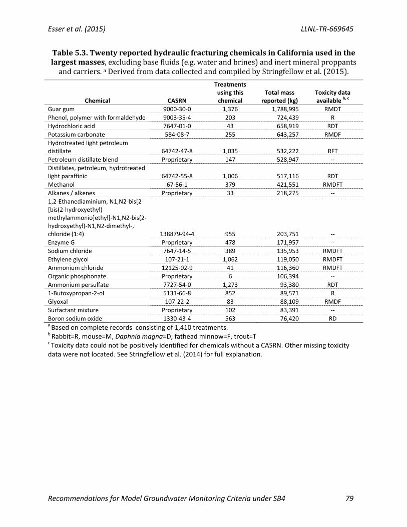
Esser et al. (2015) LLNL‐TR‐669645
Recommendations for Model Groundwater Monitoring Criteria under SB4 79
Table5.3.TwentyreportedhydraulicfracturingchemicalsinCaliforniausedinthelargestmasses,excludingbasefluids(e.g.waterandbrines)andinertmineralproppantsandcarriers.aDerivedfromdatacollectedandcompiledbyStringfellowetal.(2015).
Chemical CASRN
Treatments using this chemical
Total mass reported (kg)
Toxicity data available b, c
Guar gum 9000‐30‐0 1,376 1,788,995 RMDT
Phenol, polymer with formaldehyde 9003‐35‐4 203 724,439 R
Hydrochloric acid 7647‐01‐0 43 658,919 RDT
Potassium carbonate 584‐08‐7 255 643,257 RMDF
Hydrotreated light petroleum distillate 64742‐47‐8 1,035 532,222 RFT
Petroleum distillate blend Proprietary 147 528,947 ‐‐
Distillates, petroleum, hydrotreated light paraffinic 64742‐55‐8 1,006 517,116 RDT
Methanol 67‐56‐1 379 421,551 RMDFT
Alkanes / alkenes Proprietary 33 218,275 ‐‐
1,2‐Ethanediaminium, N1,N2‐bis[2‐[bis(2‐hydroxyethyl)methylammonio]ethyl]‐N1,N2‐bis(2‐hydroxyethyl)‐N1,N2‐dimethyl‐, chloride (1:4) 138879‐94‐4 955 203,751 ‐‐
Enzyme G Proprietary 478 171,957 ‐‐
Sodium chloride 7647‐14‐5 389 135,953 RMDFT
Ethylene glycol 107‐21‐1 1,062 119,050 RMDFT
Ammonium chloride 12125‐02‐9 41 116,360 RMDFT
Organic phosphonate Proprietary 6 106,394 ‐‐
Ammonium persulfate 7727‐54‐0 1,273 93,380 RDT
1‐Butoxypropan‐2‐ol 5131‐66‐8 852 89,571 R
Glyoxal 107‐22‐2 83 88,109 RMDF
Surfactant mixture Proprietary 102 83,391 ‐‐
Boron sodium oxide 1330‐43‐4 563 76,420 RDa Based on complete records consisting of 1,410 treatments. b Rabbit=R, mouse=M, Daphnia magna=D, fathead minnow=F, trout=T c Toxicity data could not be positively identified for chemicals without a CASRN. Other missing toxicity data were not located. See Stringfellow et al. (2014) for full explanation.

LLNL‐TR‐669645 Esser et al. (2015)
80 Recommendations for Groundwater Monitoring Criteria under SB4
Table5.4.ChemicalsreportedinDOGGRWellStimulationTreatmentDisclosureReportsnotreportedinFracFocusChemicalDisclosureRegistryasusedinCalifornia
Chemical Name CASRN Reported well stimulation
application or treatment technique
1‐Eicosene 3452‐07‐1 Matrix acidizing
Hydroxylamine hydrochloride 5470‐11‐1 Hydraulic fracturing & matrix acidizing
Acetaldol 107‐89‐1 Hydraulic fracturing & matrix acidizing
1‐Tetradecene 1120‐36‐1 Matrix acidizing
1‐Octadecene 112‐88‐9 Matrix acidizing
Ammonium fluoride 12125‐01‐8 Matrix acidizing
Benzyldimethylammonium chloride 122‐18‐9 Matrix acidizing
Lauryl hydroxysultaine 13197‐76‐7 Matrix acidizing
Benzododecinium chloride 139‐07‐1 Matrix acidizing
Miristalkonium chloride 139‐08‐2 Matrix acidizing
Nitrilotriacetic acid 139‐13‐9 Hydraulic fracturing & matrix acidizing
Fatty acids, C18‐unsatd., dimers 61788‐89‐4 Hydraulic fracturing & matrix acidizing
Amines, hydrogenated tallow alkyl, acetates 61790‐59‐8 Matrix acidizing
1‐Hexadecene 629‐73‐2 Matrix acidizing
Benzoic acid 65‐85‐0 Hydraulic fracturing & matrix acidizing
Poly(oxy‐1,2‐ethanediyl), alpha‐(nonylphenyl)‐omega‐hydroxy‐, branched, phosphates
68412‐53‐3 Hydraulic fracturing & matrix acidizing
Benzenesulfonic acid, C10‐16‐alkyl derivs., compds. with 2‐propanamine
68584‐24‐7 Matrix acidizing
Benzenesulfonic acid, C10‐16‐alkyl derivs., compds. with triethanolamine
68584‐25‐8 Matrix acidizing
Copper dichloride 7447‐39‐4 Hydraulic fracturing & matrix acidizing
Ethylene oxide 75‐21‐8 Matrix acidizing
Potassium iodide 7681‐11‐0 Hydraulic fracturing & matrix acidizing
Nitrogen 7727‐37‐9 Hydraulic fracturing & matrix acidizing
Calcium phosphate, tribasic 7758‐87‐4 Matrix acidizing
Aluminum chloride 7784‐13‐6 Hydraulic fracturing & matrix acidizing
1,3‐Propanediaminium, 2‐hydroxy‐N,N,N,N',N'‐pentamethyl‐N'‐(3‐((2‐methyl‐1‐oxo‐2‐propenyl)amino)propyl)‐, dichloride, homopolymer
86706‐87‐8 Hydraulic fracturing & matrix acidizing
‐ DOGGR Well Stimulation Treatment Disclosure Reports: data from January 1 to May 5, 2015. Such reports were required for all well stimulation treatments starting January 2015.
‐ FracFocus Chemical Disclosure Registry: chemicals not reported as used in California between 2011 and 2014.

Esser et al. (2015) LLNL‐TR‐669645
Recommendations for Model Groundwater Monitoring Criteria under SB4 81
One objective of the monitoring program is to detect potentially dangerous chemicals before they can migrate from the area of release to a “receptor,” such as a drinking water well. Unfortunately, many of the chemicals used in hydraulic fracturing and other well stimulation treatments are difficult to analyze or do not have standard analytical methods available. Monitoring programs also need to take into account that new chemicals can and are being in use in California over time and adaptive approaches to monitoring are necessary. For example, mandatory reporting under new regulations since 2015, reveals the use of chemicals that were not known to be used for well stimulation prior to 2014 (Table 5.4). Recommendations for the monitoring program include conducting specific studies examining the fate and effects of well stimulation fluid additives in the environment and making measurements of biocides and other toxic compounds that are used in well stimulation treatments. Applying “green chemistry” principles of using well characterized, less toxic and labile (non‐persistent) chemicals, where possible, could reduce the need for monitoring of specific compounds.
5.2 ChemicalUseinOtherOilandGasDevelopmentActivities Chemicals are used for a number of different purposes throughout the oil and gas production process, including drilling, well completion (during which well stimulation occurs), well cleanout, and for some types of enhanced oil recovery (EOR). In a new oil field, oil production consists of simply producing oil and gas from the reservoir (primary production). In California, production in most reservoirs has been occurring for a span of time ranging from several decades to more than a century, so primary production has ended. Continued production requires additional processes including water flooding (secondary recovery) or, in California, steam flooding or cyclic steaming (two of many types of tertiary recovery). Water flooding and steam flooding involve continuous injection to push oil toward production wells, and, in the case of steam, to also reduce the oil’s viscosity along with other effects. Cyclic steam injection involves periodic injection of steam followed by a well shut‐in period to allow the heat to reduce the oil viscosity, followed by a period of production, after which the cycle repeats (Long et al., 2015). Currently there is not a state‐wide requirement to report chemical use during oil and gas development except in the context of well stimulation, under new SB4 authorized regulations, so there is limited information on overall chemical use by the oil and gas industries. In particular, there is very little specific information on chemical use in California for EOR. A review of public literature suggests that wide spread use of polymers, surfactants, and solvents during EOR may be cost prohibitive, but information on specific practices in California were not found. The use of biocides and inhibitory agents, such as nitrate, to prevent corrosion and reservoir souring are also a common industry practice, but their specific use in California is unknown. As of June 2013, the South Coast Air Quality Monitoring District (SCAQMD) instituted mandatory reporting rules (Rule 1148.2) requiring operators to report information on chemical use for well drilling, completion, and rework operations. In a recent study, Rule 1148.2 reports

LLNL‐TR‐669645 Esser et al. (2015)
82 Recommendations for Groundwater Monitoring Criteria under SB4
to SCAQMD from June 2013 through May 2014 were examined for treatments and operations that used hydrochloric acid; it was found that over 70 other chemical compounds identified by CASRN were used in conjunction with hydrochloric acid treatments, over 20 of which were not known to be used in hydraulic fracturing (Stringfellow et al. 2015). In this report, we examined all the available records reported between the implementation of Rule 1148.2 in June 5, 2013 and February 3, 2015. Analysis of this data set showed that there is wide use of industrial chemicals in oil and gas development operations (Table 5.5). The potential environmental or groundwater hazards associated with these chemicals is unknown, but should be further investigated and considered for inclusion in the monitoring, particularly in respect to understanding legacy effects from oil and gas development. Table5.5.Numberofoilandgasproductionactivitiesandthenumberofassociateduniquematerials(chemicals,basefluids,etc.)usedintheSouthCoastAirQuality
MonitoringDistrict(SCAQMD),6/5/2013–2/3/2015.
Activity Number of identified
activities
Number of unique components used by
activity a,b
Acidizing 256 133
Hydraulic fracturing 13 67
Gravel packing 234 202
Maintenance acidizing 232 131
Matrix acidizing 7 22
Other 201 333 aBased on chemical name and CASRN. bIn all, there are 41,467 records and 943 activities. A total of 467 unique components are used.
5.3 FlowbackandProducedWaters 5.3.1 Characteristics of flowback fluids Flowback fluids consist of (1) fracturing/injection fluids pumped into the well previously, which include water and the additives, (2) new compounds that may have formed due to chemical reactions between anthropogenic additives, (3) dissolved constituents naturally present in formation waters in the target geological formation, (4) substances that have become mobilized from the target geological formation due to the interaction of fracturing fluids with formation rocks and water, and (5) some oil and/or gas (Stepan et al., 2010; NYDEC, 2011). Thus, the chemistry of flowback waters is generally different from that of the injection fluids. The composition of flowback fluids usually changes over the course of the flowback time‐period, gradually evolving from being more similar to the injection fluids to approaching the

Esser et al. (2015) LLNL‐TR‐669645
Recommendations for Model Groundwater Monitoring Criteria under SB4 83
chemical characteristics of the formation waters. For example, fluid‐composition changes were observed in studies conducted in the Marcellus shale (Hayes, 2009; Barbot et al., 2013) and the Bakken (Stepan et al., 2010), indicating concentration increases in the flowback water collected over time for constituents such as, chloride, and some cations/metals. However, these studies were based on flowback fluids collected in other states, and may not reflect the temporal patterns of flowback fluid composition in California. Chemical analysis of flowback fluids in California (referred to as “recovered fluids”) are being reported to DOGGR as part of the well completion reports. Analysis of this data is impeded by the fact that the analyses are posted as PDF files that have to be manually entered into a spreadsheet. Analysis of the data submitted in the first half of 2015 (representing operations by Aera energy in North and South Belridge) indicated that there can be high levels of total carbohydrate (possibly indicating the presence of guar), as well as other inorganic and organic constituents such as TDS, some trace elements (arsenic, selenium, and barium), NORMs and hydrocarbons in the recovered fluids (Stringfellow et al., 2015) However, as noted in section 2.2, the volume of these recovered fluids was found to be small in comparison with injection fluid volumes as well as the volumes of produced water generated in the first month of operation. Moreover, the recovered fluids can represent mixed sources of wastewater. According to the operator, the recovered fluids could be a mix of well cleanout fluids, formation water and returned stimulation fluids. Data interpretation is further complicated by the fact that operators were not required to indicate the time at which the sample was collected ((Stringfellow et al., 2015) Fracturing fluids retained in the reservoir can potentially interact with formation rocks over time. Hence, the resulting products of these fluid‐mineral interactions, which can potentially include environmental contaminants, may appear in produced waters at a later stage. While some recent studies consider the environmental risks associated with “trapped chemicals” to be low (King, 2012b), more studies are needed on the interactions of injection fluids and their additives with formation rocks and the overall fate of injection fluids in the subsurface environment, in order to determine if these have the potential to alter the chemistry of produced waters over the long term (such as causing slow release of trace metals or radioactive elements). One of the possible interactions of the injected water with the formation rock is changing the equilibrium between dissolved and exchange phases on clay minerals. The introduction of injected water with typically lower salinity into the higher saline formations could result in mobilization of elements such as boron and lithium from the exchange sites and enrichment in the flowback water (Warner et al., 2014) 5.3.2 Characteristics of produced water Once the well is placed into production, the waters recovered from the operations are “operationally defined” as “produced waters”, and primarily consist of formation water. The formation water in oil and gas reservoirs can contain naturally existing dissolved constituents such as hydrocarbons, salts, trace metals, NORMs (naturally occurring radioactive materials)
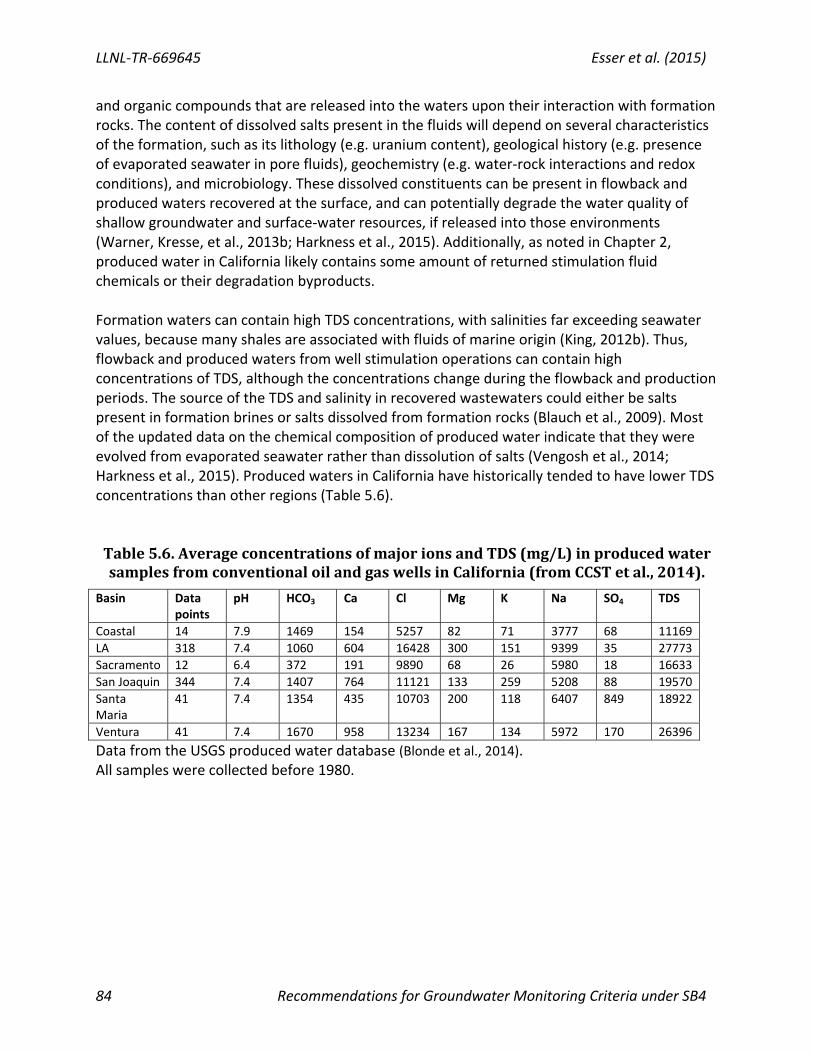
LLNL‐TR‐669645 Esser et al. (2015)
84 Recommendations for Groundwater Monitoring Criteria under SB4
and organic compounds that are released into the waters upon their interaction with formation rocks. The content of dissolved salts present in the fluids will depend on several characteristics of the formation, such as its lithology (e.g. uranium content), geological history (e.g. presence of evaporated seawater in pore fluids), geochemistry (e.g. water‐rock interactions and redox conditions), and microbiology. These dissolved constituents can be present in flowback and produced waters recovered at the surface, and can potentially degrade the water quality of shallow groundwater and surface‐water resources, if released into those environments (Warner, Kresse, et al., 2013b; Harkness et al., 2015). Additionally, as noted in Chapter 2, produced water in California likely contains some amount of returned stimulation fluid chemicals or their degradation byproducts. Formation waters can contain high TDS concentrations, with salinities far exceeding seawater values, because many shales are associated with fluids of marine origin (King, 2012b). Thus, flowback and produced waters from well stimulation operations can contain high concentrations of TDS, although the concentrations change during the flowback and production periods. The source of the TDS and salinity in recovered wastewaters could either be salts present in formation brines or salts dissolved from formation rocks (Blauch et al., 2009). Most of the updated data on the chemical composition of produced water indicate that they were evolved from evaporated seawater rather than dissolution of salts (Vengosh et al., 2014; Harkness et al., 2015). Produced waters in California have historically tended to have lower TDS concentrations than other regions (Table 5.6). Table5.6.AverageconcentrationsofmajorionsandTDS(mg/L)inproducedwatersamplesfromconventionaloilandgaswellsinCalifornia(fromCCSTetal.,2014).
Basin Data points
pH HCO3 Ca Cl Mg K Na SO4 TDS
Coastal 14 7.9 1469 154 5257 82 71 3777 68 11169
LA 318 7.4 1060 604 16428 300 151 9399 35 27773
Sacramento 12 6.4 372 191 9890 68 26 5980 18 16633
San Joaquin 344 7.4 1407 764 11121 133 259 5208 88 19570
Santa Maria
41 7.4 1354 435 10703 200 118 6407 849 18922
Ventura 41 7.4 1670 958 13234 167 134 5972 170 26396
Data from the USGS produced water database (Blonde et al., 2014). All samples were collected before 1980.

Esser et al. (2015) LLNL‐TR‐669645
Recommendations for Model Groundwater Monitoring Criteria under SB4 85
Table5.7.ComparisonofproducedwatercompositionsconventionaloilandgasoperationsinCaliforniatoproducedwaterfromconventionalandunconventional
operationsinotherregions.
TDS values ranging from 10,000 to 40,000 mg/L have been reported for the formation waters in the San Joaquin and Sacramento basins at depths ranging from ~1,500 to ~3,500 m (Kharaka et
Parameter Marcellusa Bakkenb
pH 5.1 - 8.4 5.5 - 6.5Conductivity (mS/cm) 205 - 221Alkalinity (mg/L as CaCO3) 8 - 577TSS (mg/L) 4 - 7600TDS (mg/L) 680 - 345000 150000 - 219000Chloride (mg/L) 64 - 196000 90000 - 130000Sulfate (mg/L) 0 - 1990 300 - 1000Bicarbonate (mg/L) 0 - 763 300 - 1000Bromide (mg/L) 300 - 1000Nitrate (mg/L) 5 - 802Oil and Grease-HEM (mg/L) 195 - 36600COD (mg/L) 1 - 1530TOC (mg/L)Aluminium (mg/L) NDArsenic (mg/L)Barium (mg/L) 0 - 13800 0 - 25Boron (mg/L) 40 - 192Calcium (mg/L) 38 - 41000 7540 - 13500Cadmium (mg/L)Chromium (mg/L)Copper (mg/L) NDIron (mg/L) 3 - 321 NDPotassium (mg/L) 0 - 5770Magnesium (mg/L) 17 - 2550 630 - 1750Manganese (mg/L) 4 - 10Sodium (mg/L) 69 - 117000 47100 - 74600Nickel (mg/L)Strontium (mg/L) 1 - 8460 518 - 1010Zinc (mg/L) 2 - 11Ra 226 (pCi/L) 3 - 9280Ra 228 (pCi/L) 0 - 1360U235 (pCi/L) 0 - 20U238 (pCi/L) 0 - 497Gross alpha (pCi/L) 37 - 9551Gross beta (pCi/L) 75 - 597600
a Barbot et al. (2013)b Stepan et al. (2010)c Alley et al. (2011)d Compiled for this report from the USGS Produced Water Data
Conventional Oilc
Conventional Oil and Gas (California)d
5.2 - 8.9 2.6 - 11.5
300 - 380
1000 - 8489136 - 238534 0 - 156000
0 - 148798 - 13686 0 - 12809
1 - 2 1 - 2070 - 92 0 - 18
15 - 3501 0 - 20540.0 - 0.1 0 - 2500.2 - 0.90.1 - 7.4 0 - 174
0 - 6024 - 52920 0 - 136130.0 - 0.20.1 - 1.0 0 - 2000.3 - 2.7 0 - 1000.1 - 0.5 0 - 5402 - 43 0 - 7987
2 - 5096 0 - 22601 - 8 0 - 50
405 - 126755 0 - 999203 - 10 0 - 300 - 2 0 - 6006 - 170 - 10
base 2.0 (USGS, 2014)

LLNL‐TR‐669645 Esser et al. (2015)
86 Recommendations for Groundwater Monitoring Criteria under SB4
al., 1985). A study of produced waters collected from the San Joaquin Basin found TDS of waters produced from depths <1,500 m were <4,000 mg/L (typically <2,000 mg/L), whereas waters produced from depths >1,500 m were more saline (typically >25,000 mg/L) (Fisher and Boles, 1990). This depth‐salinity pattern was found to be consistent with the transition in the basin from nonmarine strata at shallow depths to marine strata at greater depths. Since fracturing operations in California are conducted at shallower depths than in other regions ‐ e.g. more than half the wells that have been stimulated using hydraulic fracturing are within 610 m (2000 feet) of the ground surface, it is expected that TDS values of target formation waters, and hence of flowback/produced waters will be relatively low (as compared to wastewaters from stimulation operations in other regions in the United States) based on the depth‐salinity gradient patterns in the formation. The “Conventional Oil” column in Table 5.7 is from a meta‐analysis 165 oilfield analyses in the peer‐reviewed literature (Alley et al., 2011). The last column in Table 5.7 presents data on the produced water compositions from conventional oil and gas operations that have been measured in California and compiled by the USGS. The samples for which data is reported in the “USGS produced water database 2.0” (Blonde et al., 2014), were collected from conventional hydrocarbon wells before 1980. Thus these samples may not be representative of modern produced waters from conventional extraction or of produced water from well stimulation operations. More data is needed on the composition of produced waters from well stimulation operations in California to assess whether the fluid chemistries would differ significantly from conventional production. The recent DOGGR regulations for well stimulation require operators to analyze one sample 30 days after production commences, and hence would provide more insight into produced water chemistry from stimulated wells in California.
5.4 IntrinsicTracers(Geochemical,Isotopic,andGasTracers) 5.4.1 Hydrocarbons and noble gases
The molecular configuration (i.e. ratios of C1/(C2+C3)), stable isotopes of carbon (13C‐CH4) and
hydrogen (2H‐CH4) in methane, isotopes of carbons in ethane (13C‐C2), and carbon isotopes in CO2 (13C‐CO2) as well as relationships to stable carbon isotopes of dissolved inorganic carbon (13C‐DIC) and water isotopes (2H) have traditionally used to determine the origin of hydrocarbons (i.e., biogenic versus thermogenic), their evolution (e.g., maturity under closed system, mixing), and modification (e.g., reduction of CO2, biodegradation). Typically, microbial
gas is characterized by low 13C‐CH4 (<−50‰) and high C1/(C2+C3) (>1000) while thermogenic
gas has typical high 13C‐CH4 (>−50‰) and low C1/(C2+C3) (<1000). During maturation of gas,
13C systematically increase from C1 to C4 (13C‐CH4< 13C‐C2H6<
13C‐C3H8) together with decreasing gas wetness and increasing thermal maturity. Yet in unconventional shale gas, reversals or rollovers in molecular and isotopic compositions where ethane and propane
reverse the conventional trend and become isotopically lighter relative to methane (13C‐CH4> 13C‐C2H6>
13C‐C3H8) (see Golding et al., 2013 and references therein).
Esser et al. (2015) LLNL‐TR‐669645
Recommendations for Model Groundwater Monitoring Criteria under SB4 87
These geochemical and isotopic variations have been used to delineate naturally occurring hydrocarbons migration, fugitive emission, and stray gas contamination in areas of shale gas development. Osborn et al. (2011) analyzed ground water wells for 68 homes overlying the Marcellus Shale in Pennsylvania and reported higher methane concentrations for the homes,
associated with higher ethane concentrations and 13C‐CH4 consistent with a thermogenic
source. Wells located less than 1 km from the nearest shale gas well had an average 13C‐CH4 of
−37±7‰ while those located more than 1 km had an average 13C‐CH4 of −54± 11‰. Likewise, Jackson et al. (2013) analyzed additional drinking‐water wells for 141 homes in the Marcellus region of PA, providing additional evidence for a thermogenic fingerprint. It was shown that ethane was 23 times higher in homes <1 km from gas wells (P = 0.0013) and propane was detected in 10 water wells, all within approximately 1 km distance (P = 0.01). It was also shown
that drinking water wells had hydrocarbons with isotopic relationships (e.g.. 13C‐CH4>13C‐C2H6), which mimic the characteristic of a thermally post‐mature Marcellus‐like source in some wells and the upper Devonian gasses in other wells. Yet the mechanism and causes for elevated hydrocarbon gas levels in drinking‐water wells, remain highly controversial; while several studies have suggested that shale gas drilling leads to fugitive gas contamination in a subset of drinking‐water wells near drill sites (Osborn et al., 2011; R. B. Jackson et al., 2013; Darrah, Vengosh, et al., 2014; Darrah et al., 2015), others argued that methane occurrence in shallow aquifers is naturally occurring and unrelated to shale gas development (Kornacki and McCaffrey, 2011; Molofsky et al., 2013c; Baldassare et al., 2014; Siegel et al., 2015). Noble gas geochemistry provides an independent and complementary methodology for detecting the origin of hydrocarbons in groundwater that can resolve questions regarding naturally occurring versus stray gas contamination The unique properties of noble gases include: (1) non‐reactivity of the gasses from secondary processes such as microbial modification; (2) noble gases have distinct compositions in groundwater system based on the water sources. One of the sources is meteoric water originating from air‐saturated water, which contains 20Ne, 36Ar, 84Kr derived from solubility equilibrium with the atmosphere during groundwater recharge. In contrast, crustal sources are characterized by radiogenic production of noble gases such as 4He, 21Ne, and 40Ar* (sourced from 238U, 232Th, and 40 K decays) within minerals in the Earth’s crust; and (3) the differential solubility of noble gases can provide valuable information on the mode of transport in an aquifer (e.g., one‐ or two‐phase advection, diffusion, gas‐phase migration) (Ballentine et al., 1991; Onions and Ballentine, 1993; Ballentine and Burnard, 2002; Lollar and Ballentine, 2009; Darrah, Jackson, et al., 2014; Darrah et al., 2015). The distinction between naturally occurring migration of hydrocarbons and stray gas contamination from leaking of shale gas wells in aquifers overlying the Marcellus (PA) and Barnett (TX) shale formations was based on identification of two types of groundwater. The first is groundwater with elevated levels of low‐soluble noble gases 4He and 20Ne that were associated with elevated hydrocarbons (methane, ethane) and dissolved salts (Cl, Br). The enrichments of 4He and 20Ne and association with “brine” fingerprints (Warner et al., 2012a)
LLNL‐TR‐669645 Esser et al. (2015)
88 Recommendations for Groundwater Monitoring Criteria under SB4
suggest slow migration of natural gas and brines in which natural gas slowly migrates buoyantly through a water‐saturated medium (low ratios of gas to water) and 4He and 20Ne were strongly enriched in the migrating gas‐phase because of their low solubility in water (Darrah, Jackson, et al., 2014; Darrah et al., 2015). This type of groundwater was observed in wells located >1 km from gas wells and represent the naturally occurring migration of hydrocarbons in areas of shale gas development, including Salt Spring in NE PA, with high levels of methane. The second type of groundwater was identified in drinking water wells located less than 1 km from shale gas wells and had high levels of hydrocarbons with no correlations with crustal (4He) or brine components (Cl, Br) and had also low concentrations Ne, Ar, and other atmospheric gases (e.g., N2, Kr). The depletion of atmospheric gases in water could occur from migration of a large gas volume through water and partition of the atmospheric gases in bubble phase, termed “stripping.” This noble gas distribution enabled Darrah et al. (2014) to distinguish the impact of stray gas contamination in a subset of wells where the elevated hydrocarbons were associated with the noble gas “stripped” composition. Given that each noble gas (He, Ne, Ar, Kr, Xe) has a unique solubility and diffusion constant, their isotopes fractionate to different extents during their co‐transport with hydrocarbons through the water‐saturated crust. Consequently, the different fractionation patterns and ratios to hydrocarbons (e.g., 4He/CH4) are controlled by the mode of transportation such as diffusion (extreme enrichment of helium in the migrated gas‐phase), two‐phase advection (extreme enrichment of both helium and neon in the migrated gas‐phase), or as a free gas (progressively less enrichment of the light gases with increasingly higher volumes of gas to water increases). Darrah et al. (2014) suggested that the lack of gas fractionation in the majority of wells with a “stripping” composition located less than 1 km from shale gas wells indicate that extremely large volumes of thermogenic hydrocarbon gases were migrated to shallow aquifers without interacting with the water‐saturated aquifer during the transport. Given that migration of gas directly from underlying shale formation would require transport through saturated rocks, these findings exclude the possibility of large‐scale gas migration from depth following hydraulic stimulation but rather indicate the majority of the stray gas contamination occurred from “free gas” leaking of shale gas wells (Darrah, Jackson, et al., 2014; Darrah et al., 2015). Overall, the integration of hydrocarbon geochemistry, stable isotopes of carbon and hydrogen in different hydrocarbons and CO2, and noble gas geochemistry could provide a strong diagnostic tool for detecting stray gas contamination. The cumulative research in PA and TX sites (R. B. Jackson et al., 2013; T. Darrah et al., 2014)(R. B. Jackson et al., 2013; T. Darrah et al., 2014) and Canada (Muehlenbachs, 2012) indicate that leaked gas from oil and gas wells is not always characterized by a thermogenic fingerprint identical to the gas in the shale formations since leaking can also be derived through the well annulus from other geological formations overlying the shales. Hence integration of all available geochemical tools is essential for adequate evaluation of the occurrence of hydrocarbons in groundwater resources.

Esser et al. (2015) LLNL‐TR‐669645
Recommendations for Model Groundwater Monitoring Criteria under SB4 89
5.4.2 Water Chemistry Groundwater contamination from oil and gas simulation and hydraulic fracturing can be the result of leaking of the oil and gas wells, flow of the hydraulic fracturing fluids and formation waters through the fractures generated from hydraulic fracturing, and from surface activities (e.g., storage, transport, spills, leakage of the oil and gas wastewater and solids) (Jackson et al., 2014; Vengosh et al., 2014). The total dissolved solid (TDS) content of produced water in the US ranges from roughly seawater (35,000 mg/L) to over 10 times more saline than seawater, depending on the shale formation. Produced waters in the Fayetteville (25,000 mg/L), Barnett (60,000 mg/L), Woodford (110,000‐120,000 mg/L), Haynesville (110,000‐120,000 mg/L), Marcellus (up to 180,000 mg/L) and Bakken (300,000 mg/L) shales vary by nearly an order of magnitude (Warner et al., 2012a; Haluszczak et al., 2013; Warner, Kresse, et al., 2013b; Barbot et al., 2013; Vengosh et al., 2014; Rowan et al., 2015). In California, data available from USGS suggest that produced water from geological formation overlying the Monterey Formation has TDS up to 35,000 mg/L.
5.4.2.1 Geochemical Fingerprints Typically, produced water from conventional and unconventional oil and gas wells mimic the composition of modified evaporated seawater, with high Br/Cl and low Na/Cl (relative to seawater ratios) and high Ca/Cl ratios (Warner et al., 2012a; Haluszczak et al., 2013). Flowback waters from the Marcellus and Fayetteville shales are characterized by high B/Cl and Li/Cl ratios that reflect mobilization of lithium and boron from clay minerals in the shales (Warner et al., 2014). Preliminary USGS data indicate that produced water from both conventional and hydraulically fractured wells in Belridge Field in Central Valley in California have high Br/Cl ratios but also high Na/Cl, which is not consistent with the conventional model of evaporated seawater. The preliminary data also show very high boron and lithium contents as well as high B/Cl and Li/Cl ratios that far exceed the ratios expected from evaporated seawater. Furthermore produced waters from both hydraulic fracturing and conventional oil and gas operations are characterized by high dissolved inorganic carbon (DIC) that it is not common in produced water from shale gas basins. One of the challenges in evaluating the impact of oil and gas operations is the distinction between salinization of shallow groundwater from the flow of deep saline groundwater (e.g., north‐eastern Appalachian Basin; Warner et al., 2012a) and direct contamination induced from oil and gas operations. The monitoring program should be designed to include geochemical and hydrogeological characterization of the multiple aquifer systems adjacent to oil and gas fields and utilize as many geochemical and isotopic diagnostic tools as possible for delineating the specific impact of oil and gas operations in California.
5.4.2.2 Oxygen and Hydrogen Isotopes Stable isotopes of oxygen and hydrogen most commonly vary conservatively in groundwater systems and hence have used extensively in groundwater studies. The stable isotopes of oxygen and hydrogen in water can be used to evaluate the evolution of brines associated with oil and gas operations (i.e. dilution versus original evaporated seawater), to evaluate regional

LLNL‐TR‐669645 Esser et al. (2015)
90 Recommendations for Groundwater Monitoring Criteria under SB4
groundwater flow, and to provide insights on the sources of contaminants. Evaporated
seawater and brines in oilfield formation waters are typically characterized by higher 18O and 2H values than meteoric waters and shallow groundwaters containing meteoric waters. The isotopic composition of water produced from oilfields will be affected by the isotopic composition of the formation fluids and of water and steam injected for enhanced oil recovery. Both steam and water injected for enhanced oil recovery or well stimulation are likely to be lighter than formation water. The difference in isotopic composition between produced water and shallow groundwater has been used to identify isotopically heavier or “enriched” wastewater percolating from a produced water pond into the shallow unconfined aquifer at Lost Hills (California CVRWQCB, 2012). Given that injected water and steam, produced waters, and shallow and deep groundwaters are all likely to have distinct isotopic compositions, the stable isotopic composition of oxygen and hydrogen in groundwater may be a useful tracer of impact from produced or injected water.
5.4.2.3 Boron Isotopes
Boron has two stable isotopes (11B/10B ratio ~4) whose ratio varies extensively in nature due to the large fractionation of relatively light isotopes. The boron isotope ratio has been used to trace groundwater contaminants such as agricultural runoff, wastewater, and petroleum waste. The boron isotope ratio is controlled by the exchange reaction of boron species where 11B is enriched in boric acid while 10B is fractionated into the borate ion that is typically removed to the solid phase (e.g., adsorption, co‐precipitation in carbonate minerals). The boron isotope
fractionation generates a large 11B [11B =(11B/10Bsample / 11B/10B SRM951 ‐1) x10
3] variation, up to 100‰, that enables researchers to delineate boron sources (e.g., marine versus non‐marine, seawater intrusion versus domestic wastewater, oil brines versus coal effluents) and processes (adsorption versus desorption). Flowback fluids from the Marcellus and Fayetteville shales are
characterized by relatively low 11B (26‐31‰) compared to produced water from conventional
oil and gas wells with typically high 11B (>39‰; Warner et al., 2014). The relatively lower 11B in flowback waters was explained by desorption process of boron from the shale deposits
during hydraulic fracturing process while high 11B reflect adsorption of seawater boron onto clay minerals with selective 10B removal (Warner et al., 2014). A previous study of the Monterey Formation has revealed elevated boron concentrations (50 to 150 mg/L) in pore water (Carpenter and Moore, 1997), which is consistent with preliminary USGS data of high boron (up to 73 mg/L) in oil and gas produced water from Belridge Field. The high boron in the pore water was explained by the transformation of the boron‐rich diatomite to boron‐poor opal CT, and boron released by the dissolution of diatomaceous silica is not co‐precipitated with silica in
opal‐CT (Carpenter and Moore, 1997). Given the low 11B measured in DSDP cherts (‐9‰ to +8‰; Kolodny and Chaussidon, 2004) it is expected that formation waters associated with
siliceous rocks (i.e., opal CT) would have a lower 11B signature relative to fluids interact directly with marine shales in the Monterey Formation (>25‰).

Esser et al. (2015) LLNL‐TR‐669645
Recommendations for Model Groundwater Monitoring Criteria under SB4 91
5.4.2.4 Lithium Isotopes Lithium (6Li 7.5% and 7Li 92.5%) is a fluid‐mobile element and, due to the large relative mass difference between its two stable isotopes, is subject to significant low temperature mass fractionation, which provides key information on the nature of water‐rock interaction
processes. Recent studies have shown that the range of 7Li values spans more than 40‰ at
the Earth surface [7Li = (7Li/6Lisample / 7Li/6LiL‐SVEC ‐1) x10
3]. Lithium isotopes are strongly fractionated during secondary mineral formation such as alteration of clay minerals (e.g., illitization) and weathering processes. The variations of lithium isotopes in hydrologic systems depend on the intensity of water/rock interactions both in terms of temperature in geothermal systems and “weathering regime” in surface waters. The common controlling mechanism of lithium isotope compositions is the balance between dissolution of primary minerals and the formation of secondary minerals. Flowback fluids from the Marcellus and Fayetteville shales are
characterized by relatively low 7Li (6‐10‰) compared to produced water from conventional oil
and gas wells with typically high 7Li (8‐25‰; Warner et al., 2014). The relatively lower 7Li in flowback waters was explained by desorption of lithium from the shale deposits during
hydraulic fracturing process while high 7Li in conventional oil and gas produced water reflect adsorption of seawater lithium onto clay minerals with selective 6Li removal (Warner et al., 2014).
5.4.2.5 Strontium Isotopes
The variations of strontium isotopes (87Sr/86Sr) in hydrological systems typically mimic the compositions of the host geological formations due to the lack of isotope fractionation between solid and dissolved strontium. It has been shown that Middle Devonian Marcellus brine has a distinctive 87Sr/86Sr ratio (~0.7114) relative to produced water from the Upper Devonian formation in the Appalachian basin (0.716‐0.722; Chapman et al., 2012; Warner et al., 2012a; Kolesar Kohl et al., 2014). The distinctive strontium isotope ratios of the Marcellus brines was used to delineate the origin of saline groundwater in shallow aquifers in north‐eastern PA and link them to possible upflow of deep saline water that originated from migration of the Marcellus brines (Warner et al., 2012a). It also enabled researchers to detect the origin of wastewater discharged to a stream in western PA and link it shale gas drilling (Warner, Kresse, et al., 2013b). Preliminary USGS data suggest that produced waters from Central Valley in California have 87Sr/86Sr range of 0.70806 to 0.70913. Given the high influence of the matrix rocks on the Sr isotope composition of the coexisting brines, mapping and establishing Sr isotope database along a geological cross section could help in reconstructing the variations of Sr isotopes of groundwater from different geological formations and the possible isotopic differences relative to the produced waters from oil and gas operations.
5.4.2.6 Carbon isotopes in Dissolved Inorganic Carbon
The stable carbon isotopes in DIC (13C‐DIC) could provide important information on DIC sources as well as different processes such as redox processes associated with methane oxidation by sulfate‐reducing bacteria or methanotrophic bacteria or archaea, leading to

LLNL‐TR‐669645 Esser et al. (2015)
92 Recommendations for Groundwater Monitoring Criteria under SB4
characteristic fingerprints of 13C‐ depleted DIC. While DIC is not a conservative constituent in groundwater system and would be strongly affected by water‐rock interactions, it could help to evaluate different processes associated with oil and gas contamination, in particular secondary processes such as sulfate reduction associated with stray gas contamination. The carbon isotopes in DIC could also help to distinguish between produced waters originated from
hydraulic fracturing relative to steam‐simulation since low 13C‐DIC composition is expected during steam extraction.
5.4.2.7 Radium Isotopes
The occurrence of radium nuclides in produced and hydraulic fracturing waters is important given the high toxicity of radium to human health. The two major radium isotopes are 226Ra with a half‐life of 1600 years and 228Ra with much shorter half‐life of 5.6 years. Produced and flowback waters from the Marcellus Formation are characterized by elevated levels of radium nuclides (Warner, Kresse, et al., 2013b; Rowan et al., 2015). The magnitude of radium adsorption is inversely correlated with salinity and thus dilution of the radium‐rich fluids would enhance radium adsorption onto stream sediments in disposal and/or leaking sites. Long‐term disposal of treated wastewater originating from both conventional and unconventional oil and gas production in western PA had caused massive radium accumulation on stream sediments downstream of disposal sites (Warner, Kresse, et al., 2013b). It has shown that Marcellus brines have a distinctive low 228Ra/226Ra ratio (~0.3) relative to produced water from conventional oil and gas wells in the Appalachian Basin (228Ra/226Ra~1; Rowan et al., 2015) and thus can be used to identify the source of the wastewater and the accumulated radium in river sediments. Preliminary radium isotope data from produced waters from Belridge Field in Central Valley in California show radium activity of several magnitudes lower than activity reported in the Marcellus brines.
5.5 IntroducedTracers The California Department of Conservation Draft Environmental Impact Report on oil and gas well stimulation (California DOC and Aspen Environmental Group, 2015) identifies an “inability to identify specific impact to groundwater quality from well stimulation activity” as a groundwater impact, and recommends as a mitigation measure the addition of a tracer to well stimulation fluids or the development of a reasonable method to distinguish well stimulation treatment fluids in the environment. Tracers, to date, have not been introduced to injected fluids for the express purpose of monitoring protected groundwater for impact from well stimulation treatment. 5.5.1 Desirable properties of added tracers for evaluating groundwater impacts of hydraulic
fracturing Chemical and radioactive tracers are commonly used in oilfield applications to investigate reservoir properties, fracture network interconnectivity, and well‐to‐well communication, and

Esser et al. (2015) LLNL‐TR‐669645
Recommendations for Model Groundwater Monitoring Criteria under SB4 93
to verify well integrity (Serres‐Piole et al., 2012). More recently, gamma‐emitting, tracer‐labeled proppant has been combined with geophysical logging to evaluate proppant delivery and stimulated well integrity in unconventional high‐volume hydrofracture wells (King, 2011). For the purpose of using tracers to evaluate groundwater impacts of hydraulic fracturing operations, the following properties are desirable:
High specificity and uniqueness relative to native and anthropogenic compounds expected in the local environment,
Conservative behavior,
Detectability at low concentrations, and
Low toxicity or other negative environmental effects. High specificity and uniqueness of the tracer would be extremely useful for correlating hydrofracture fluid impacts to particular well stimulation events, and for distinguishing these impacts from legacy effects of oilfield wastewater discharges to unlined sumps or injection into underground injection control (UIC) wells. Among the characteristics ideally associated with conservative behavior are transport with injected water, stability (chemical, biological, and thermal), and inertness (e.g., with respect to physicochemical interactions with the solid matrix, such as sorption and ion exchange). The ability for sensitive detection enables early detection of tracers in advance of contaminants that may adversely affect protected aquifers. 5.5.2 Potential candidates for use as introduced tracers for evaluating groundwater impacts There are currently not tracers that conform well to all of the above characteristics and whose performance has been extensively field‐validated in the hydraulic fracturing context. Nonetheless, some promising technologies are discussed below. Synthetic DNA oligomers are relatively short DNA molecules composed of, for example, less than 200 base pairs. They have considerable promise for this application as they conform well to the ideal characteristics listed above. In terms of specificity and uniqueness, even a short DNA oligomer can carry an extraordinarily distinctive signature and a massive amount of information; for example, a 50‐base‐pair DNA molecule could have on the order of 1030 possible unique sequences. An advantage of this high level of uniqueness is that well‐specific tracers could be added to many different wells in a given area and could provide distinctive information on water‐borne constituents deriving from each well. Highly sensitive, specific, and quantitative detection of DNA oligomers is possible with quantitative polymerase chain reaction (qPCR) analysis, which is standard in modern biological laboratories and can detect fewer than 5 or 10 copies of a specific DNA target in a sample. DNA is nontoxic, provided that it does not encode a harmful peptide, which can be ensured in the design of the tracer (e.g., tracer sequences could be designed to be different from any known gene sequences, including virulence genes). DNA is also water soluble, and has been shown in a hydrological study to have aquifer transport behavior similar to a bromide tracer (Sabir et al., 1999); a hydrological study in surface water also confirmed that DNA tracers had similar transport behavior to injected chloride, but the DNA tracer mass was substantially reduced due to undefined processes
LLNL‐TR‐669645 Esser et al. (2015)
94 Recommendations for Groundwater Monitoring Criteria under SB4
(Foppen et al., 2011). The DNA tracer technology has been commercialized (BaseTrace, Research Triangle Park, NC) but its performance under conditions of hydraulic fracturing has not been extensively studied or documented, although the CEO, Justine Chow, has stated that the synthetic DNA oligomers are resistant to high temperature, high salinity, shear forces, and UV exposure (the latter is relevant to storage in surface impoundment ponds) (Ritter, 2014). Considering the range of reactive chemicals (e.g., strong oxidants and electrophilic compounds like glutaraldehyde) and harsh conditions (e.g., acidic conditions) that typically exist in well stimulation fluids, the stability of DNA tracers is not guaranteed, and even minor chemical changes could potentially interfere with detection by qPCR. Thus, DNA tracers have high potential but they still require field validation studies under relevant conditions. Fluorescent dye tracing is a standard, proven groundwater tracing technology (e.g., Serres‐Piole et al., 2012) and one of the most commonly used methods in groundwater tracing experiments. Fluorescein dye has a number of favorable properties as an added tracer including the following: it is inexpensive to purchase and analyze, is easy to detect at low concentrations (e.g., at the ng/L level for spectrofluorimetry), it has good thermal stability, and it is relatively nontoxic (Serres‐Piole et al., 2012). Its disadvantages include that it can sorb to solids and is susceptible to biological degradation, so is best suited to short‐term field tests (Serres‐Piole et al., 2012). Superparamagnetic metal oxide nanoparticles are another emerging class of tracers that have been proposed for use in a hydraulic fracturing context (Revkin, 2013; Ritter, 2014). The nanoparticle surfaces have been coated with a proprietary short‐chain organic zwitterionic species that acts as a surfactant to facilitate uniform dispersion of the particles in stimulation fluids (Ritter, 2014). The nanoparticles are designed to exhibit specific magnetic signatures by virtue of specific combinations and ratios of certain elements (iron/manganese/zinc or iron/gadolinium/aluminum) in their cores (Ritter, 2014). Nanoparticle tracers have been commercialized by FracEnsure (Pearland, TX). Andrew Barron, a co‐founder of FracEnsure, stated that the Texas‐based Southwestern Energy would begin testing the nanoparticles in hydraulic fracturing wells in late 2014 (Ritter, 2014). Note: The authors of this report have no affiliation with or financial interest in the companies or technologies discussed in this section.
5.6 SamplingMethods In the pursuit of groundwater monitoring for WST impacts through proper pre‐drilling baseline and post‐ stimulation monitoring, there are issues around the questions: what is a representative sample and what does a sample represent in the spatial and temporal contexts? There has been no discussion of these issues in the WST or broader literature concerning oil and gas development in the stray gas context. We introduce the topic here as one that deserves much attention as pilot projects are designed for WST monitoring. Analytical detection limits

Esser et al. (2015) LLNL‐TR‐669645
Recommendations for Model Groundwater Monitoring Criteria under SB4 95
for groundwater samples submitted to laboratories typically receive much attention but what the sample actually represents relative to the questions being addressed does not. The water represented by the sample sent to the lab for analysis is a blend or mixture of waters from various geologic layers in the zone or hydrogeologic unit being sampled. For example the chemical composition of a sample from a monitoring well with a one foot long well intake (the length of the granular pack around the well screen) in an aquifer is likely different than what would be obtained if the well intake is 10 or 50 feet long. The selection of the length of the monitor interval is important. The degree of difference depends on the degree of heterogeneity in the system. What constitutes a relatively long intake on a monitoring well or internal in a multilevel monitoring system depends on the spatial scale of the hydrogeology and the contaminant source. A long intake allows more of the vertical dimension to be sampled but increases the blending, which may dilute the contamination in a thin zone below detection. The trend in groundwater monitoring for contamination in general is towards shorter well intakes and more wells in the cluster or more monitor intervals in the multilevel system. Long monitor intakes can cause early detection of contaminant plumes to be missed as contaminant concentrations early on are diluted below detection. For stray gas monitoring in groundwater the pathways and the spatial and temporal characteristics of gas plumes are not known and therefore the needed framework for quantitative consideration of monitor intake lengths does not exist. The length of monitor intake chosen will depend on the stated purpose of the monitoring. Monitor intake lengths for receptor and sentry monitoring will differ from monitor intake lengths for detection or performance monitoring. Currently, we do not have sufficient knowledge of subsurface heterogeneity in protected groundwater aquifers overlying California oil and gas fields or of contaminant transport pathways and mechanisms to determine the optimal monitor intake length for detection or performance monitoring of well stimulation in California. The second important fundamental decision concerning groundwater sampling is the method by which the sample is taken. There are three options: aggressive purging (pumping) before sample collection, low‐flow sampling (minimal pumping to take the sample, not purge the system) and point sampling such as SNAP sampling, diffusion bag sampling or use of other down hole water collectors without pumps. In this approach, the water taken by the sampler or the chemicals collected in the diffusion bag come from a small volume domain in the intake internal. The aggressive purging method draws water to the well from various domains in the formation and mixes the water so that the sample is a blended average weighted towards the most permeable zones near the well. In contrast to that, the outer two methods rely on groundwater flow to bring the water to the sampling point with minimal but likely some blending due to vertical flow in the intake interval if the interval is not quite short. The trend in groundwater sampling for contamination is away from aggressive purging. The use of low flow or the" no pumping" sample methods generally reduces cost and avoid large scale blending for which the effects are little understood. The merits of these three sampling options have not been assessed in the WST context and the transferability of assessments for other types of groundwater contamination issues is limited by the nature of the question concerning stray gas.
LLNL‐TR‐669645 Esser et al. (2015)
96 Recommendations for Groundwater Monitoring Criteria under SB4
5.7 Detectingimpactandestablishingbaseline Impact to groundwater from WST can be detected by observing changes in downgradient water quality. The USEPA (2009) document “Statistical Analysis of Groundwater Monitoring Data at RCRA Facilities: Unified Guidance” was developed for use in Resource Conservation and Recovery Act (RCRA) contexts. However, the basic purpose is the same and the methods are applicable to post‐WST monitoring. USEPA (2009) is based on the premise that a geographic region has been defined and that within that region:
a) one or more wells has been selected, from which samples of groundwater can be collected,
b) one or more constituents has been identified, c) impacts to groundwater will cause (persistent) changes in concentrations for one or
more constituents at one or more of the wells. USEPA (2009) describes several methods for detecting change. The “prediction limit with retesting” strategy (Chapter 19 of USEPA 2009) is likely to be a cost effective choice. Several variations of the strategy are available. The version outlined here is the “1 of 3” strategy. More generally, strategies of this type are referred to as “1 of m” strategies; USEPA (2009) recommends m of no greater than 4. Conceptually, these strategies are much like using control charts, but the calculations of the limits and the interpretation of results are different (control chart methods do not employ retests). The statistical theory underlying these method is complex, but software with which to implement it is available. Using baseline data, a statistical upper prediction limit (PL) is calculated for each well/constituent pair. During each subsequent sampling period (e.g., every 6 months) the following steps are followed for each well/constituent pair.
1. A single initial sample is collected and analyzed. 2. If the initial sample result is below the PL then the constituent/well pair “passes” and no
further action based on that well/constituent pair is necessary. 3. If the initial sample result is above the PL, then two “retest samples” are collected,
starting as soon as possible, and spaced far enough apart in time to provide statistical independence between samples.
4. If either of the retest sample results is below the PL then the constituent/well pair passes, and no further action is necessary.
5. If both retest samples are above the PL then the three results together are considered to be statistical evidence of an increase in average concentration.

Esser et al. (2015) LLNL‐TR‐669645
Recommendations for Model Groundwater Monitoring Criteria under SB4 97
Key features of this strategy include:
The “m” in “1 of m” means that at most m samples will be collected in any sampling period.
The (m‐1) retests will be collected sequentially, and if a retest sample passes then any remaining retest samples need not be collected or analyzed.
Adjustments are made if there are constituents that are not detected in any baseline sample.
USEPA (2009) suggests that retest analyses be done only for constituent(s) that did not pass in the initial sample.
The method assumes that long‐term average concentration of each constituent in baseline water is constant. If it can be established that there is no spatial variation in average concentration across the area, then it would be possible to compare downgradient results with a PL calculated from an upgradient well or from a combination of upgradient and downgradient wells. For regions where spatial variation exists or where spatial uniformity cannot be established, well/constituent pairs from baseline sampling of that well can be used. From a statistical point of view, a program of this type jointly includes all of the downgradient wells and constituents/indicators in the area, and is thus more efficient than a program that treats each well/constituent pair independently. The method is designed to balance the need to detect impacts promptly with the desire to avoid having too many false positives (where “false positive” refers to deciding that the average concentration has increased when in fact it has not). The Unified Guidances (USEPA, 2009) discusses how retesting significantly reduces the false positive rate Application of the method to area‐specific monitoring under SB4 will have to address two issues. The first is the long legacy of oil and gas production in California. Monitoring wells may be installed in oilfields that have been operating for many decades, and historic oilfield operations may have impacted water quality in overlying groundwater aquifers. In these cases, “baseline” will not refer to pristine conditions but rather to conditions as they exist before the WST event, and these conditions may be affected by legacy impacts. The second is that the method relies on detecting changes in analyte concentrations outside of the normal range in variation as defined by repeated analyses of samples under baseline conditions. The composition of groundwaters overlying oilfields in California is often not well known and more than one pre‐WST analysis may not be available. In these cases, the use of semi‐annual sampling for a reasonable period of time after the WST event should be explored as a method for establishing baseline. Establishing what constitutes a reasonable period of time would require estimating transit time for groundwater and for free gas in groundwater. As the program evolves, more information and analyses will become available for establishing temporal and spatial variability in baseline conditions.

LLNL‐TR‐669645 Esser et al. (2015)
98 Recommendations for Groundwater Monitoring Criteria under SB4
Statistical evidence of an increase in concentration for a single or multiple analytes does not automatically indicate an impact to protected water from the WST, especially when baseline conditions are not well established. Additional assessments by the State (presumably in cooperation with the Operator) would determine whether additional monitoring or corrective action is necessary.

Esser et al. (2015) LLNL‐TR‐669645
Recommendations for Model Groundwater Monitoring Criteria under SB4 99
6 RECOMMENDATIONSFORAREA‐SPECIFICMONITORING
6.1 DiscussionofRecommendationsforArea‐SpecificMonitoring On September 21, 2013, California passed Senate Bill 4 (Pavley, 2013). The Bill requires the State Water Board to develop groundwater monitoring model criteria on or before July 1, 2015 for inclusion in Water Code section 10783. In the interim period, CA DOGGR put in place interim emergency regulations (Cal. Code Regs. tit. 14, § 1783.4 (2014)) requiring groundwater sampling, testing, and monitoring related to well stimulation that is conducted prior to the finalization of model groundwater monitoring criteria by the State Water Board. The final regulations adopted by DOGGR require documentation from either the State Water Board or the Regional Water Board that the well subject to the well stimulation treatment is covered by a groundwater monitoring plan in accordance with Water Code section 10783. The following recommendation “Groundwater Sampling, Testing, and Monitoring for Hydraulic Fracture or Acid Well Stimulations Where Protected Groundwater is Present” expands on the interim emergency regulation (Cal. Code Regs. tit. 14, § 1783.4 (2014)) and lays out requirements for a groundwater monitoring plan for a stimulated well or tightly clustered set of stimulated wells. The recommendation satisfies the SB4 requirement for expert advice on the development of groundwater monitoring criteria on a well‐by‐well spatial scale. Throughout the document, we use “area‐specific” monitoring to refer to both area and “well‐by‐well” monitoring. In a densely drilled oil and gas field where stimulation wells are closely spaced, a groundwater monitoring well may serve to monitor more than one stimulated well, and a groundwater monitoring plan may encompass more than one stimulated well. These recommendations propose requirements for the submission of information on local hydrogeology, including the distribution of groundwater salinity and gas content. The intent is to require information that can be used to develop a site conceptual model of the potential transport of fluids from the stimulated zone and well to protected groundwater. The discussion below is not meant to be comprehensive or to provide a rationale for every area‐specific recommendation proposed in the following discussion. Rather, it addresses the overall monitoring approach adopted in the recommendation, and discusses the major recommendations. 6.1.1 Groundwater monitoring of well stimulation in California SB4 requires groundwater monitoring of oil and gas wells subject to WST “in order to protect all waters designated for beneficial uses” with priority to monitoring groundwater that has the

LLNL‐TR‐669645 Esser et al. (2015)
100 Recommendations for Groundwater Monitoring Criteria under SB4
potential to be a source of drinking water. The legislation further requires that “in order to assess the potential effects of well stimulation treatments on the State’s groundwater resources in a systematic way, the State Board develop model groundwater monitoring model criteria” that address a range spatial scales from individual oil and gas well monitoring to regional monitoring. The recommendations in this chapter address model criteria for monitoring an individual oil and gas well or a group of oil and gas wells subject to well stimulation treatment. The challenges in designing a groundwater quality monitoring network for well stimulation in California on either an area‐specific or regional scale are enormous. Oil and gas well stimulation occurs at depths that are generally deeper than protected groundwater resources. While the stratigraphy of shallow fresh water zones and deeper oil and gas zones is often known, information relevant to contaminant transport in intervening zones, including protected groundwater between 3,000 and 10,000 mg/L TDS and intervening confining layers, is often not available. Oilfields, especially those where enhanced oil recovery is practiced, are dynamic with temporally and spatially variable pressure gradients. In fields with long histories of development, legacy impacts on overlying protected groundwater resources may complicate detection of impact from current operations. These fields may also contain active, inactive or abandoned wells in close proximity to the stimulated well being monitored; and the integrity of these nearby wells may or may not be known. All of the factors combine to make designing a site‐specific and risk‐based groundwater monitoring network extremely difficult. Adding to the challenge is that very few examples exist where purposeful groundwater monitoring networks for shale gas or any other types of well stimulation activities have been created to assess impacts on the groundwater resource (e.g., Hammack et al., 2014), and no examples exist where such networks are required by a regulatory program. There have been several expert panel reports concerning the environmental impacts of shale gas development issued in the USA, Canada, Australia and Europe since 2011 (summarized in CCA and Cherry, 2014) and all have recommended that groundwater monitoring should be done to assess the subsurface impacts of shale gas development. However none has indicated where and how such monitoring should be accomplished. Whatever information exists about the impacts of petroleum resource development comes from the sampling of household wells, farm wells, municipal wells and springs in the areas of the petroleum resource developments. This type of groundwater monitoring (e.g., domestic well sampling) is common in regions of shale gas and shale oil development in the United States and Canada because it serves to establish baseline conditions most relevant to potential litigation from claims of damage to private or public water‐supply‐wells. However sampling of existing water wells provide little advance warning of impending impacts on groundwater resources, nor does it provide much insight about the nature of the groundwater system to identify potential pathways and long‐term cumulative impacts. Given the lack of precedents, the most effective means to developing a well‐founded groundwater monitoring approach to well stimulation in California is to first conduct field‐
Esser et al. (2015) LLNL‐TR‐669645
Recommendations for Model Groundwater Monitoring Criteria under SB4 101
based pilot projects to provide the science and identify, and if necessary develop, the technology to support the development of guidance and regulations for when and in what manner to conduct groundwater monitoring of stimulation operations. The pilot projects would need to use a combination of established and innovative methods and therefore at least in part would need to be established as research projects. We recommend that these projects be implemented under the Regional Groundwater Monitoring Plan. SB4 requires, however, that well‐by‐well groundwater monitoring be conducted for all new well stimulation projects. The challenge then is to develop a scientifically credible approach to this permit‐required monitoring in the absence of experience from similar programs elsewhere in the nation or world. Designing a groundwater monitoring network involves answering certain questions about the placement of groundwater monitoring wells, schedules and protocol for groundwater sampling and water quality analysis:
Where: Where should groundwater samples be collected? How far from the WST zone should samples be collected, both laterally and vertically? From how many depths should samples be collected?
When: When should groundwater samples be collected? How frequently? For how long?
What: What type of monitoring instrumentation is most appropriate? What chemicals and other parameters should be analyzed for?
The design of a groundwater monitoring network (i.e. the answers to these questions) is contingent on the purpose of the groundwater monitoring. Several types of groundwater monitoring exist (CCA, 2014).
“Receptor” monitoring: Receptor monitoring is direct monitoring of the resource (e.g. a water supply well or aquifer) to assess impact from one or more sources or activities. Baseline monitoring is required to demonstrate a change in water quality in subsequent monitoring which should be performed on a time scale that considers contaminant transport processes. SB4 requires that monitoring be offered for water supply wells within 1,500 feet of a stimulated wellhead. This requirement is not discussed in these recommendations. SB4 also requires monitoring of protected groundwater aquifers.
“Sentry” monitoring: Sentry monitoring is done between a source and a receptor (e.g., water supply well) along a contaminant pathway. Sentry monitoring is generally implemented to protect a valuable or sensitive receptor by detecting impacts before they reach the receptor. We recommend installation of a guard well between the stimulated well and the water supply when the water supply well is within one mile of a stimulated well.
“Detection” monitoring: Detection monitoring is designed to detect water quality impacts on an ongoing basis from a specific source or industrial process. Detection

LLNL‐TR‐669645 Esser et al. (2015)
102 Recommendations for Groundwater Monitoring Criteria under SB4
monitoring is commonly used to determine if municipal landfills are performing as designed or are “leaking”. In the context of well stimulation treatment, such monitoring would be designed to demonstrate if a specific oil and gas well subject to well stimulation treatment performed as designed or “leaked”, i.e. whether or not injected fluids, chemical additives, produced waters, oil or gas from a specific oil and gas well subject to well stimulation remained zonally isolated from protected groundwater or alternatively impacted protected groundwater.
“Assessment” or “compliance” monitoring: Assessment monitoring takes place after an impact has been detected or is suspected and is designed to characterize the extent and magnitude of the impact. Interim regulations under DOGGR and our recommendations have provision for contingency plans, which potentially include the installation of monitoring wells to define and localize water quality impacts to protected groundwater when stimulated well integrity is compromised or an unintended event occurs that could impact protected groundwater quality.
We discuss permit‐required monitoring in the context of different groundwater monitoring systems below. Detection monitoring: Groundwater quality monitoring may not be the best strategy for assessing zonal isolation of injected or produced fluids from individual oil and gas wells subject to stimulation. Requiring detection monitoring of individual oil and gas wells runs the risk of making the same mistakes made in groundwater monitoring programs at industrial sites in North America in the 1980s and 1990s. Routine groundwater monitoring was mandated by US EPA at contaminated sites in the late 1970s, before key field research in contaminant hydrogeology was performed. Routine monitoring was implemented in accordance with the new regulations, using spatially‐distributed, single‐interval monitoring wells, which were thought to be appropriate given the conceptual models of subsurface contamination at the time. University and government field research subsequently showed that dissolved contaminants migrate differently than initially assumed (i.e., hydrodynamic dispersion of contaminants is highly variable and dependent on site specific conditions, including preferential pathways), and that the conventional monitoring well networks often yielded ambiguous results. Modern groundwater monitoring technologies and methods, which consider the factors listed above, yield much more definitive monitoring results. Currently, detection monitoring networks in shallow groundwater underlying surficial waste management sites such as landfills commonly involve tens of wells over relatively small spatial scales. In addition to issues of the scale, detection monitoring of groundwater potentially impacted by well stimulation is impractical at this point in time because of our lack of knowledge and detailed understanding of complex hydrogeologic systems, especially migration pathways through those portions of the system that separate oil and gas production zones from protected groundwater. The state of science and experience in how best to develop effective groundwater detection monitoring for oil and gas operations is poorly developed. To date, most groundwater monitoring data for well stimulation have come predominantly from existing water supply wells that were not designed for detection monitoring.

Esser et al. (2015) LLNL‐TR‐669645
Recommendations for Model Groundwater Monitoring Criteria under SB4 103
As a consequence, we do not recommend using groundwater monitoring wells for early detection monitoring of individual WST wells at this time. Other methods not in the scope of these recommendations (which concern groundwater monitoring), including real‐time pressure monitoring of the stimulated well during the well stimulation event and short‐lived radioactive tracer tests to detect major loss of fluids out of the stimulated zone, reported spills in transport or storage of fluids at the wellhead, and monitoring of gas leakage at the wellhead (through monitoring sustained case pressure or soil gas) are better and more immediate indicators of major loss of well integrity or the occurrence of unintended events that could compromise water quality in protected groundwater aquifers. These alternative approaches alone, however, do not preclude subsurface leakage that could have discernable impact on groundwater quality and therefore do not eliminate the need for groundwater quality monitoring. Real‐time pressure monitoring may not detect minor fluid loss under certain circumstances, and even minor losses of fluid could negatively impact groundwater quality, especially in densely drilled fields with a long history of development. Wellhead monitoring of gas or of annulus pressure will not rule out leakage into the protected groundwater zone. Deeper monitoring along the well casing may be an effective form of monitoring capable of addressing wellbore leakage. Research into this type of performance monitoring, however, is at an early stage, and consequently this type of monitoring is not recommended as a requirement of groundwater monitoring under SB4 at this time. Focused field‐based pilot studies are required to understand how best to implement such a system. Receptor monitoring and the importance of baseline: If we define receptors to include not just existing wells but also the protected groundwater resource, then the installation of groundwater monitoring wells in aquifers potentially impacted by WST operations is a form of receptor monitoring. The goal here is not detection of impact early enough to allow mitigation or localized enough to assess performance of an individual stimulation operation, but rather demonstration and attribution of impact of well stimulation on a protected groundwater aquifer. Critical to demonstrating impact is having adequate characterization of baseline water quality, including spatial and temporal variability. Establishing baseline and baseline variability for chemical constituents that occur naturally and for oil and gas related chemical constituents in areas with a long history of oil and gas development where groundwater quality may be impacted by legacy operations is crucial. Methane or stray gas is an example. Methane occurs naturally, and the methane in a water supply well can be biogenic or thermogenic in origin with a concentration at a particular time dependent on transient conditions such as water table depth, rainfall, pumping cycles and the depth in the well from where the sample is collected. Insufficient baseline characterization of concentration and isotopic composition of methane in shallow groundwater has complicated interpretation of methane occurrence in domestic water supply wells outside of California. The recent draft EPA Assessment of the Potential Impacts of Hydraulic Fracturing for Oil and Gas on Drinking Water Resources (USEPA, 2015b) states that “baseline data on local water quality is needed to quantify changes to drinking water resources and to provide insights into
LLNL‐TR‐669645 Esser et al. (2015)
104 Recommendations for Groundwater Monitoring Criteria under SB4
whether nearby hydraulic fracturing activities may have caused any detected changes” and states that a limitation of the assessment is “insufficient pre‐ and post‐hydraulic fracturing data on the quality of drinking water resources”. And indeed, some of the criticism of the EPA report has been the lack of a prospective study. In California, groundwater quality in aquifers overlying oil and gas fields is poorly characterized, especially for protected groundwaters with 3,000‐10,000 mg/L TDS. Installation of monitoring wells in proximity to stimulated wells will provide the data necessary to assess baseline water quality of protected groundwater and to assess its temporal and spatial variability. Particularly important will be assessing legacy impacts on current water quality. Assessing legacy impacts is important for a number of reasons, including to establish a baseline for detecting future impacts from permitted operations, especially if an unintended event occurs during a well stimulation with the potential to impact water quality triggers additional monitoring under a contingency plan. It will be important under this scenario to know if certain compounds or geochemical signatures indicative of fluids associated with well stimulations are present or absent in protected groundwater as the result of legacy operations. Additionally, characterizing the spatial and temporal variability in groundwater quality is critical for developing a defensible metric for detecting future impacts. A second reason for assessing legacy impact is the opportunity it provides for assessing the success of zonal isolation as a regulatory approach. Historically, regulation of oil and gas development in California has focused on well construction and oilfield operation standards that have been developed to assure zonal isolation. And zonal isolation over and beyond the lifetime of the well is still the first and the most important line of defense against impact. Without water quality data from potentially impacted aquifers, however, the degree to which legacy oil and gas operations have isolated overlying protected groundwaters from fluids injected into or produced from oil and gas zones is difficult to evaluate, and yet such an assessment is essential to “allaying the public’s concerns regarding well stimulation treatments of oil and gas wells”, a stated goal of the SB4 mandate for groundwater monitoring. An additional benefit of area‐specific monitoring will be in characterizing the spatial distribution of groundwater resources with a defined beneficial use. The occurrence and depth distribution of groundwaters with between 3,000 and 10,000 mg/L, in particular, is poorly known. Sentry monitoring: Sentry monitoring is designed to provide warning that contaminants have escaped from the resource development site (the gas or oil well) and are approaching a receptor. The sentry monitoring needs to be positioned so that there is early enough detection to allow decisions to protect the receptors by corrective actions or in the case of threatened wells, alternative water supplies may need to be provided. We make two recommendations in the spirit of sentry monitoring. The first is to require a guard well between the stimulated well and any domestic, municipal or agricultural water supply well within 1 mile of the stimulated well, with the guard well to be screened across the main transmissive section of the water supply aquifer. The second recommendation is to monitor the

Esser et al. (2015) LLNL‐TR‐669645
Recommendations for Model Groundwater Monitoring Criteria under SB4 105
base of the protected groundwater zone in order to detect upward migration of formation fluids or transport of well stimulation fluids that might impact shallower higher quality and/or more accessible groundwater resources. Both of these recommendations make simplistic assumptions about contaminant migration pathways and will likely only detect relatively large impacts. Assessment monitoring: Assessment monitoring is designed to confirm and characterize the extent of impact to water quality from a specific event (e.g., a spill or casing breach). Compared to detection monitoring, assessment monitoring generally requires additional monitoring locations and more frequent analysis of a longer list of required analytes. We make no specific recommendations with regard to assessment monitoring in this document beyond recommending that operators submit a contingency plan for reporting information in the event of a well failure, or any other unintended event that has the potential to affect groundwater quality, such as the detection of an induced fracture beyond the ADSV or into protected waters. We also recommend that in response to the potential release, the operator and the appropriate Regional Water Quality Control Board work together to develop a groundwater investigation and corrective action plan, including groundwater samples to be collected from existing groundwater monitoring wells, installation of additional groundwater monitoring wells, and specialty analyses to be conducted based on any stimulation tracers and end‐member chemistry (e.g., hydrofracture fluids, “flowback,” and produced reservoir fluids). 6.1.2 Protected groundwater We define protected groundwater as groundwater of less than 10,000 mg/L TDS in an aquifer that produces water in sufficient quantity for beneficial use and that is not excluded from groundwater monitoring by written concurrence from the State or Regional Water Board. California is in the midst of a historic drought and any water with the potential for beneficial use should be protected. The limit of 10,000 mg/L TDS aligns with federal regulations concerning Underground Injection Control and is technically feasible to desalinate. The USGS Discussion Paper (Taylor et al., 2014) lists over a dozen plants that currently or will soon desalinate brackish groundwater. The recommendation for area‐specific groundwater monitoring includes submission of information relevant to the distribution and determination of groundwater salinity in areas where stimulation is common. We also recommend factors to be considered in reviewing requests for exclusion from groundwater monitoring. We use the aquifer exemption criteria under the UIC program (CFR Tit. 40 § 146.4) as a template. For the UIC program, the US EPA regulatory approach is to couple a broad definition of covered (i.e., protected) underground waters to a discretionary exemption mechanism in order to protect underground sources of drinking water while also allowing underground injection associated with industrial activities including the production of minerals, oil, or geothermal energy. Exempting an aquifer from the protections afforded an Underground Source of Drinking Water (USDW), however, differs from excluding an aquifer from the requirement that its water quality be monitored. Since groundwater monitoring alone does not preclude industrial activities, we recommend expanding the definition of covered waters to

LLNL‐TR‐669645 Esser et al. (2015)
106 Recommendations for Groundwater Monitoring Criteria under SB4
encompass waters used as a source of beneficial use and applying a more stringent standard for exclusion from monitoring. In the proposed language for exclusion from groundwater monitoring, we have made the following modifications to the Exempt Aquifer criteria.
Changed “source of drinking water” to “source of water for beneficial use”,
Eliminated the depth and location criteria;
Eliminated the Class III well mining criterion;
Replaced the 3,000‐10,000 mg/L criterion with a >10,000 mg/L criterion, and
Modified the hydrocarbon production criterion to specify that only waters in hydrocarbon production zones that are >10,000 mg/L can be considered for exclusion from groundwater monitoring.
The last change is motivated by concern with the use of produced water from stimulated wells for non‐industrial activity beneficial uses such as agricultural irrigation. Such use is admirable and should be encouraged in times of drought. Current monitoring requirements for such waters, however, may not be sufficient to detect chemical additives in water produced from stimulated wells. To address this issue, such as when produced water from a stimulated well is used for agricultural irrigation, we recommend ongoing monitoring of that produced water. More specifically, we recommend not excluding groundwater from hydrocarbon producing zones that contains less than 10,000 mg/L TDS from area‐specific groundwater monitoring. This monitoring may take the form of sampling and testing produced water rather than from separate groundwater monitoring wells. We specifically do not exempt hydrocarbon‐bearing groundwaters or produced water used for agricultural irrigation (e.g., the Cawelo Water District’s use of produced water from Chevron oil and gas operations to provide irrigation for almonds and pistachios) from monitoring. Hydrocarbons can be and are removed from saline produced waters to allow for beneficial use in enhanced oil recovery (Frankiewicz, 2015) and in agricultural irrigation. We recommend monitoring produced water of less than 10,000 mg/L TDS on the same semi‐annual schedule and with the same tiered analytical approach as for protected groundwaters. We do not require, however, the installation of additional monitoring wells or locations in the hydrocarbon producing formation. We recommend that all protected groundwater be monitored by either the area‐specific or regional groundwater monitoring programs. For area‐specific monitoring, we recommend that monitoring well locations be within one half mile of the stimulated well with individual monitoring of each protected aquifer (with short‐screened clustered monitoring wells or with a multi‐level sampling system). Given that the purpose of the monitoring is protection of groundwater resources, we also make a specific recommendation for the installation of guard wells when water supply wells are in close proximity to the stimulated well. This is a stronger standard than simple monitoring of supply well water quality.

Esser et al. (2015) LLNL‐TR‐669645
Recommendations for Model Groundwater Monitoring Criteria under SB4 107
6.1.3 Risk‐based groundwater monitoring We recommend that monitoring be tiered on the basis of the quality of the groundwater being protected and on the risk of a release of stimulation fluid or produced water into protected groundwater. Higher quality water (groundwater with less than 3,000 mg/L TDS that qualifies for a municipal or domestic water supply beneficial use) should be monitored more intensively than lower‐quality water (groundwater with between 3,000 and 10,000 mg/L TDS that qualifies as protected groundwater). Well stimulations that are in close proximity to other wells (especially those with unknown well integrity) and/or to fault traces have higher risk of release to protected groundwater and should be monitored more intensively than well stimulations that are not in close proximity to other wells or transmissive geologic features. To identify a distance that qualifies as “in close proximity, we use and modify the concept of Axial Dimensional Stimulation Areas (ADSA) as defined in DOGGR regulation. DOGGR’s well construction standards are more protective of water with <3,000 mg/L than >3,000 mg/L TDS. Consequently water with 3,000 to 10,000 mg/L TDS is at greater risk of impact from leakage due to stimulation. Consequently monitoring this groundwater is the second priority.
6.1.3.1 Axial Dimensional Stimulation Volume (ADSV) Given that one of the more significant potential contaminant pathways is transmission through wellbores or faults in close proximity to the stimulated well, we also recommend for the purpose of identifying potential pathways that a conservative estimate of the extent and orientation of fracturing during well stimulation be used. The final text of the Division of Oil, Gas, and Geothermal Resources regulations (Chapter 4, Article 4, 1781(f)) defines Axial Dimensional Stimulation Area (ADSA) as the estimated axial dimensions, expressed as maximum length, width, height, and azimuth, of the area(s) stimulated by a well stimulation treatment. No reference is made in this definition to uncertainty in dimensions and in particular to azimuthal uncertainty. In addition, the ADSA as defined is a volume and not an area. Although fracture azimuth can often be successfully predicted, a conservative estimate of ADSA assumes that the fracture azimuth is not known with the consequence that the ADSA becomes a cylindrical volume (Figure 6.1a). To avoid confusion with the DOGGR definition of ADSA, we refer in this document to Axial Dimensional Stimulation Volume (ADSV). Predicting fracture azimuth requires that both the stress orientations and magnitudes be understood at the depth of stimulation and in adjacent underburden and overburden zones. If an operator wishes to argue for a specific fracture azimuth, they will need to provide the data and analysis that were used to determine the expected azimuth. In particular, not just the orientations but the magnitudes of the principal stresses and any associated uncertainties must be quantified. In environments where the stresses are close in magnitude (most commonly the two horizontal stresses in practice) induced fractures may only have a weak tendency to follow the principal stress directions as they propagate laterally. Note that typical practice is to

LLNL‐TR‐669645 Esser et al. (2015)
108 Recommendations for Groundwater Monitoring Criteria under SB4
assume that the vertical stress is one of the principal stresses (this is generally regarded as a robust assumption at depth away from significant surface topography). The magnitude of vertical stress is then obtained through integration of the formation density, derived from a density log, through the overburden thickness. The orientations of the lateral stresses are then obtained via analysis of borehole damage (drilling induced fractures and breakouts). The minimum stress (one of the horizontal stresses for normal and strike‐slip stress environments) can be quantified by a minifrac test. However, estimating the maximum horizontal stress is often problematic because there is no established reliable means to measure it directly. In practice, the value of the maximum horizontal stress is bounded via various observations of wellbore failure modes. For this reason, the operator should clearly document the methods used to infer the value and uncertainty of the maximum horizontal stress. Should the minimum and maximum horizontal stresses be potentially similar within the uncertainties, no azimuthal prediction can be made reliably. Alternatively, in the absence of sufficient quantification of the three principal stresses, previous experience demonstrating that monitored stimulations (for example, via induced microseismicity) reliably follow the same trend in similar geologic materials in close proximity and at the same depth could be used to argue for a specific hydraulic fracture orientation. However, in this instance, the operator will need to demonstrate that the current stimulation operation and siting does not differ significantly from established experience. There is evidence that some locations in California experience more complicated stress environments, especially adjacent to larger faults in stronger strata. In such locales, hydraulic fractures may tend to propagate with more of a horizontal or intermediate orientation. It is important to recognize that the vertical extent of the ADSV is a key parameter in determining the potential threat to protected waters. Our recommendation is that operators be required to provide detailed evidence (either results of pilot studies/other prior experience or models calibrated to vetted data) to support the proposed vertical extent of the ADSV. Typically the vertical extent of a hydraulic fracture is estimated by models that assume fractures are contained by variations in the lateral stresses with depth. It is largely assumed that the fracture will extend upward to an interval where the confining stress is of sufficient magnitude to inhibit continued fracture propagation (a so called, “stress barrier”). Depending upon the quality of the data in the model, the robustness and reliability of the stress barrier may be marginal. For this reason, we propose that a conservative estimate of the maximum potential vertical growth of a hydraulic fracture would be to consider the largest linear dimension (lateral or vertical) of the ADSV to be used as an estimate of the potential vertical extent of the fracture.

Esser et al. (2015) LLNL‐TR‐669645
Recommendations for Model Groundwater Monitoring Criteria under SB4 109
Figure 6.1a. A view of ADSV showing predicted induced fracture dimensions including zone of azimuthal uncertainty based on field data provided by Operator. Well 1 is located within the 2xADSV zone of azimuthal uncertainty; Well 2 is located within the 2xADSV cylindrical volume but outside the zone of azimuthal uncertainty; Well 3 is located within 1xADSV cylindrical volume but outside the zone of azimuthal uncertainty; Well 4 is located outside the 2xADSV cylindrical volume. Graphics by Sascha Madrid.

LLNL‐TR‐669645 Esser et al. (2015)
110 Recommendations for Groundwater Monitoring Criteria under SB4
Figure 6.1b. Stimulated well with multiple stages, each with an individual cylindrical ADSV. The 2xADSV height of the composite ADSV uses the height of the shallowest stage to determine the upper bound of the composite 2xADSV volume. Graphics by Sascha Madrid. We recommend a conservative definition of ADSV unless the operator submits field data relevant to stress orientation and fracture azimuth for a given strata being stimulated along with a fracture azimuth and azimuthal uncertainty. We also make clear that the calculation of the height of the 2xADSV volume for a vertical multi‐stage well is based on the height of the envelope of individual ADSV heights closest to protected groundwater, which will typically be the shallowest stage. (Figure 6.1b). In addition, as mentioned previously, the estimated vertical extent of the fracture should be based upon the maximum extent of the ADSV for added conservatism to allow for the possibility that stress barriers do not perform as intended.

Esser et al. (2015) LLNL‐TR‐669645
Recommendations for Model Groundwater Monitoring Criteria under SB4 111
In defining whether or not a well or fault is in close proximity to a stimulated volume, we recommend identifying wells within twice the ADSV and transmissive features (such as faults) within five times the ADSV, in accord with DOGGR’s regulations. The volume of concern is larger for geologic features because the location of such features is typically known with less precision and accuracy than well location. These features also may extend further than the area in which they are detected. For instance, faults are often detected from seismic reflection surveys. These surveys have a detection limit with regard to fault offset that is measured in meters. Because of this, the area of fault offset extends some distance beyond where the fault is detected.
6.1.3.2 Tiered monitoring on the basis of water quality and risk We recommend risk‐based monitoring in which the intensity of monitoring is determined by the risk of impact to the protected groundwater resource. The science of assessing risk to groundwater from well stimulation is still in its infancy. Focused field studies are urgently needed to understand transport of oil and gas field fluids out of zone, to understand the factors that control risk to groundwater, and to understand how best to monitor well stimulation. Our recommendations are based on the current state of knowledge. Trigger for the requirement to develop an area‐specific groundwater monitoring plan: Our recommendation is that an areas‐specific groundwater monitoring plan be required when protected groundwater is within ½ mile of a stimulated well. SB4 only requires groundwater monitoring when a stimulated well “penetrates” a protected groundwater resource, and so our recommendation to monitor protected groundwater within ½ mile of a stimulated well will not always be enforceable. We feel, however, that the recommendation is more protective of groundwater with beneficial use. The above criteria are consistent with SB4 guidance to prioritize monitoring of groundwater that has the potential to be a source of drinking water. Assessment of risk of well stimulation to protected groundwater: Our recommendation for monitoring of protected groundwater for impact from well stimulation considers three risk factors: the vertical separation between the base of protected groundwater and the stimulated zone, the presence of potential pathways (wells and transmissive geologic features) in close proximity to the stimulated well, and the density of previously stimulated wells in the immediate vicinity of the stimulated well (Table 6.1).

LLNL‐TR‐669645 Esser et al. (2015)
112 Recommendations for Groundwater Monitoring Criteria under SB4
Table6.1:Riskfactorsandgroundwatermonitoring
Vertical Separation
Pathways in close proximity
Previous WST within 0.5
mile
Aquifers monitored and # locations per aquifer Type of
well High‐Quality Freshwater
Base of Freshwater
Deep protected
>2xADSV+ 100 ft
None known
<4 3 0 0 Regional or Area
4 to 50 3 0 3
>50 3 3 3
Potential
<4 3 0 3
Area 4 to 50 3 0 3
>50 ≥3 ≥3 ≥3
Likely Additional review required. WST may not be allowed or additional monitoring of at‐risk aquifers may be required
≤2xADSV+ 100 ft
WST not allowed
‐ Vertical separation is the vertical distance from the top of well interval stimulation to the base of the deepest aquifer with protected groundwater
o ADSV for determination of vertical separation uses the maximum stimulated volume dimension o 2xADSV is selected to provide a safety factor with respect to actual extent relative to the predicted
extent of the stimulation o An additional 100 feet of vertical separation is specified to assure sufficient aquitard thickness
remains un‐breached if a stimulation extends 2xADSV vertically
‐ Pathways in close proximity refers to existing wells or geologic features close to the stimulated well o “None known” indicates no known wells within 2xADSV or geologic features within 5xADSV of the
stimulated well o “Potential” pathways include adequately sealed or abandoned wells within 2xADSV or geologic
features not known to be transmissive within 5xADSV of the stimulated well o “Likely” pathways include inadequately sealed or abandoned wells within 2xASDV or geologic
features known to be transmissive within 5xADSV of the stimulated well
‐ Prior WST density refers to the number of previously stimulated wells within a ½ mile radius of the proposed location for the stimulated well
o 3 wells in a 0.5 mi. radius area is about 160‐acre spacing; o 51 wells in a 0.5 mi. radius area is about a 10‐acre spacing and corresponds to two infill patterns
more than a 160‐acre spacing
‐ Aquifers monitored refers to the protected groundwater aquifers that must be monitored in the groundwater monitoring plan
o “High‐Quality Freshwater” refers to an aquifer within the freshwater (0‐3,000 mg/L) zone with the highest quality water within the zone as defined by having the minimum salinity in the zone.
o “Base of freshwater” refers to an aquifer within and near the base of freshwater (0‐3,000 mg/L) zone o “Deep protected” refers to an aquifer at the base of the protected groundwater zone o The number (0, 3, or ≥3) refers to the number of monitor locations for each aquifer monitored. This
will generally be one upgradient and two downgradient.
‐ Type of Well refers to the distance allowed between the stimulated well and the monitor location o “Regional” wells are wells installed by the Regional Groundwater Monitoring Program. These wells,
when allowed as a monitoring location in an Area‐Specific Groundwater Monitoring Plan, must be screened in an appropriate aquifer and may be up to one mile from the stimulated well
o “Area” wells are wells installed by the operator and must be screened in the appropriate aquifer and must be within ½ mile of the stimulated well.
Esser et al. (2015) LLNL‐TR‐669645
Recommendations for Model Groundwater Monitoring Criteria under SB4 113
Vertical separation between the stimulated zone and the base or top of protected groundwater: To reduce the risk of induced fractures propagating into the protected groundwater zone, we recommend that a minimum vertical separation between the protected groundwater zone and the stimulated zone be required before well stimulation is allowed to proceed. We set this separation at twice the longest dimension of the ADSV and add an additional one hundred feet as a safety factor. The use of the longest dimension of the ADSA or ADSV is recommended to provide a margin of safety for future large‐volume hydrofractures in which lateral dimension may be significantly greater than vertical dimension. Potential pathways in close proximity to the stimulated well: After wastewater disposal through surface discharge or subsurface injection, the most likely scenario by which well stimulation could impact protected groundwater is through a fracture network intersecting an existing well or transmissive geologic feature with subsequent transport of fluids to a protected groundwater aquifer. In recognition of this, we use the proximity of existing wells or potentially transmissive geologic features to the stimulated well as a primary determinant of risk of protected groundwater impact and the level of groundwater monitoring required. Other factors may also affect risk to protected groundwater, including the mass of fluid and the mass and identity of chemical additives injected, the density and age of existing wells within a region, vertical separation and the competence of caprock or confining layers between the protected groundwater zone and the hydrocarbon‐producing zone. The Board may wish to incorporate these factors more fully into regulation in the future. Some of these factors (vertical separation, well density) are considered in our recommendations, but we use the presence and integrity of existing wells within close proximity to stimulated wells as a primary factor in our recommendation. We assign the lowest risk to those stimulated wells that are not in close proximity to existing wells or geologic features, intermediate risk to those stimulated wells in close proximity to existing wells in that are properly sealed or abandoned or in close proximity to potentially transmissive geologic features, and highest risk to stimulated wells in close proximity to existing wells that cannot be documented or tested to be properly sealed or abandoned or an in close proximity to geologic features known to be transmissive. An example of a known transmissive geologic feature is a fault in the Santa Barbara Channel that is a pathway for gas to seep from reservoirs to the sea bed (Boles et al., 2010). While no protected groundwater is in the vicinity of this particular example, it is likely similar features exist on land, but they are easier to detect underwater. For existing wells within 2xADSV of a stimulated well, the probability that they could act as a pathway through which protected groundwater could be impacted is significantly reduced when they are adequately cased and cemented or abandoned. “Adequate” sealing and abandonment in this context means expanding on current DOGGR regulations for casing, cementing and abandonment. For instance, while DOGGR’s field rules regarding well construction typically require a continuous cement seal in the outer annulus from the ground surface to an aquitard below the deepest aquifer containing groundwater with ≤3,000 mg/L

LLNL‐TR‐669645 Esser et al. (2015)
114 Recommendations for Groundwater Monitoring Criteria under SB4
TDS, we recommend the Board require well seals compliant with the Groundwater Protection Standard in the Draft Environmental Impact Report (California DOC and Aspen Environmental Group, 2015). This requires that “the annular space between the well casing and the subsurface be sealed with cement to fill the annular space to a confining unit below groundwater with 10,000 mg/L TDS water”, meaning cementing the outer annular space along the entire length of casing from a regional seal or aquitard below the base of protected groundwater to the ground surface. DOGGR regulations also require cementing the outer annular space at least 500 above oil and gas zones, such as that targeted for stimulation. We recommend this seal should extend 500 feet, or into a regional seal or aquitard above more than 2xADSV (Figure 6.2). These recommendations are designed to prevent wells from compromising zonal isolation as a result of the lack of cement or proper casing or proper abandonment within the protected groundwater zone. Existing wells within 2xADSV of stimulated well that meet the above standard would be assessed as potential pathways. Existing wells within 2xADSV of stimulated well that do not meet or cannot be demonstrated to meet the above standard would be assessed as likely pathways. Confirmation that an existing well meets the standard will require a combination of documentation and/or testing. Documentation would include well design, construction and completion; and results from any mechanical integrity testing or cement bond logging performed on the well. Testing would include mechanical integrity testing to demonstrate that the annular cement seals in wells in close proximity to the stimulated well will prevent unintended migration of fluid, cement bond logging, or other suitable measurements. In the event that the well is already plugged, there is no rigorous method currently available to determine the integrity of the plugging operation other than documentation of the means used to abandon the well. Any such documentation should be provided and if the abandonment procedures are deemed to be insufficient, the well shall be presumed to be a potential pathway. In the event that the quality of the abandoned well cannot be ascertained, it should be presumed to act as a likely pathway. Remedial action (e.g. cementing or abandonment of inactive wells) should be encouraged to reduce risk. We recommend that a similar review be made of geologic features that could potentially act as contaminant pathway. Geologic features will be presumed to be potential pathways unless they are known to be transmissive, in which case they will be assumed to be likely pathways. In the event that the 2xADSV boundaries of a proposed well stimulation overlap with the 2xADSV boundaries of a previous well stimulation, we recommend that the previously stimulated well and pathways associated with the previously stimulated well be considered as potential pathways for the proposed well stimulation and that risk be assessed accordingly. In the event that an ADSV was not developed for previous neighboring well stimulations, we recommend allowing a reasonable estimate be used in its place (e.g., through comparison with comparable WST operations in the area). We believe that the risk of transmission through overlapping stimulated fractures into a well or geologic feature that is not in close proximity to

Esser et al. (2015) LLNL‐TR‐669645
Recommendations for Model Groundwater Monitoring Criteria under SB4 115
the proposed stimulated well is smaller by an unknown but significant degree than the risk of transmission through stimulated fractures into a well or geologic feature that is in close proximity to the proposed stimulated well.
Figure 6.2. Minimum annular seal requirements for active or idle wells within 2xADSV of a stimulated well. The dashed box shows the projection of 2xADSV from nearby stimulated well. These requirements are consistent with the Groundwater Protection Standard proposed in the Draft Environmental Impact Report (California Department of Conservation and Aspen Environmental Group, 2015). Note requirement to extend annular cement seal at the base of the production casing to a regional seal (i.e., aquitard) that is at least 100 feet above the top of 2xADSV. Graphics by Sascha Madrid.

LLNL‐TR‐669645 Esser et al. (2015)
116 Recommendations for Groundwater Monitoring Criteria under SB4
Figure 6.3a. Number of wells within ½ mile of each well in the predominantly hydraulically fractured pools in southeastern Kern County (Appendix N, Long et al., 2015). Each of these wells has a high probability of having been hydraulically fractured. Note that for purposes of visualization, the number of wells in proximity was mapped to the Thiessen polygon for each well, rather than to a point representing the well.

Esser et al. (2015) LLNL‐TR‐669645
Recommendations for Model Groundwater Monitoring Criteria under SB4 117
Figure 6.3b. Number of other hydraulic fracturing operations with 0.5 mile of hydraulic fracture wells in the predominantly hydraulically‐fractured pools (accounting for cover ~90% of the hydraulic fracturing operations in the state). Density of previous well stimulations. The density of previously stimulated wells in close proximity to the stimulated well being monitored (Figure 6.3) is also a risk factor. Because numerous studies have found that a certain fraction of wells leak (e.g., Dusseault et al., 2000), a single exploratory well poses less of a threat to protected groundwater than do numerous wells in a densely drilled field. Everything else being equal, risk to protected groundwater in a particular area scales approximately with the number of stimulations that occur in that area (recognizing that this relationship may depart from linear with increasing aggregate risk). As shown in Figure 6.3, peak stimulated well densities in California exceed 1,000 well stimulations per square kilometer and vary by three orders of magnitude. Figure 6.3a shows the distribution of stimulations by the number of stimulations within ½ mile based on the analysis presented in Figure 6.3. In the predominantly hydraulic fractured pools analyzed, few well stimulations occur in areas of low stimulation density. In all pools, the fraction of well stimulations in areas of low stimulation density will only be slightly higher because relatively few stimulations occur outside the predominantly hydraulic fractured pools analyzed.
LLNL‐TR‐669645 Esser et al. (2015)
118 Recommendations for Groundwater Monitoring Criteria under SB4
We recommending categorization of new stimulated wells based on the number of previously stimulated wells within ½ mile radius of the stimulated well using three broad categories: <4, 4 to 50, and >50 previously stimulated wells. The least dense spacing (<4 previously stimulated wells within ½ mile radius of a new stimulated well) corresponds to an exploration well. Tiered groundwater monitoring: For all new stimulated wells (with one exception) we recommend monitoring at least two aquifers: a freshwater (0‐3,000 mg/L) aquifer with the highest quality water (i.e., lowest TDS) and a protected groundwater (3‐10,000 mg/L) aquifer nearest the stimulated zone. High‐quality freshwater aquifers are the most likely to be used for domestic, municipal or agricultural water supply and are the most sensitive to degradation. Protected groundwater aquifers closest to the stimulated zone (which will commonly be aquifers near the base of protected groundwater or more rarely aquifers near the top of a protected groundwater zone underlying a hydrocarbon producing zone) will be the first to be impacted by transport of injected fluids through transmissive geologic features or by upwelling or migration of formation fluids out of the hydrocarbon‐producing zone to shallower or deeper protected groundwater zones through a breach in caprock or confining layers. For exploratory stimulated wells with less than 4 previously stimulated wells within ½ mile radius and with no existing wells or geologic features within 2xADSV, we recommend only requiring monitoring of the freshwater aquifer. For stimulated wells in higher density fields (i.e., wells with >50 previously stimulated wells within ½ mile), we recommend requiring monitoring of an additional third aquifer at the base of freshwater (0‐3,000 mg/L). For low‐risk stimulated wells with no existing wells or geologic features in close proximity, we recommend allowing the use of either area‐specific monitoring wells with ½ mile or appropriately‐screened regional wells within 1 mile – these distances are discussed in greater detail in following section on groundwater monitoring design. For all other stimulated wells, we recommend requiring the use of area‐specific wells within ½ mile of the stimulated well. As will be discussed, for each aquifer monitored, we recommend requiring one upgradient and two downgradient locations. For stimulated wells in high‐density fields (i.e., with more than 50 previously stimulated wells within ½ mile), we recommend requiring more than three monitor locations at the discretion of the Water Board. Legacy impacts in densely drilled fields may result in spatially variable water quality in protected groundwater aquifers and require more monitoring wells to adequately characterize the spatial variability. For proposed stimulated wells in close proximity to likely pathways, i.e. to geologic features known to be transmissive or to existing wells that cannot be demonstrated to be properly sealed or abandoned, we recommend additional review of existing well integrity and transmissive geologic features, site‐specific hydrogeology, and current and potential future use of the aquifers. Based on an assessment of risk, we recommend not allowing well stimulation to proceed unless existing wells are properly sealed or allowing well stimulation to proceed with monitoring of additional aquifers. For example, if an existing well was known to not be

Esser et al. (2015) LLNL‐TR‐669645
Recommendations for Model Groundwater Monitoring Criteria under SB4 119
cemented through the 3,000‐10,000 mg/L zone, the Water Board could require either that the well be remediated to meet the standard or that all major aquifers in the 3,000‐10,000 mg/L protected groundwater zone be monitored. Additional monitoring could also be based on the potential future use – the Water Board could require monitoring all major aquifers with less than 3,000 mg/L (the limit for designation of domestic or municipal water supply beneficial use) or all major aquifers with less than 1,500 mg/L (the short‐term upper limit for drinking water).
Figure 6.4. A view showing one monitoring location with the installation of three conventional groundwater monitoring wells or one multi‐level system well. Graphics by Sascha Madrid.
LLNL‐TR‐669645 Esser et al. (2015)
120 Recommendations for Groundwater Monitoring Criteria under SB4
6.1.4 Groundwater monitoring design
6.1.4.1 Groundwater monitoring systems For each aquifer monitored, we recommend two downgradient and one upgradient monitoring well. We recommend that groundwater monitoring plans include standard hydrogeologic information relevant to determining hydraulic gradient direction and magnitude under unstressed, and, if available, stressed conditions. In all cases, determination of gradient and siting of monitoring wells in the proposed groundwater management plan should be prepared by a California‐certified Professional Geologist, Certified Hydrogeologist or Professional Engineer and be based on geologic and hydrologic information supplied in the groundwater monitoring plan. We acknowledge that much of the requested information may not be available, especially for deeper aquifers. Hydraulic gradients in the 3,000‐10,000 mg/L protected groundwater zone, in particular, are unlikely to be well characterized or discernable from available information. If a gradient cannot be determined, deep wells may be sited with shallow wells in a well cluster or engineered multi‐level monitoring system. The recommended requirement for two downgradient wells and one upgradient well in each monitored aquifer is a minimal configuration. Traditionally, the requirement for two downgradient wells was to account for uncertainty in groundwater gradient in a performance or detection groundwater monitoring network. Current practice, however, has demonstrated that two downgradient wells are generally inadequate to meet the goals of detection monitoring for shallow aquifers underlying well‐characterized surface sources. The challenges for detection monitoring of a WST well, where leakage through a well integrity failure can occur along thousands of feet of casing and cement across complex hydrogeology including multiple aquifers with poorly defined hydraulic properties are significant. Such complexity cannot be addressed by two downgradient wells and one upgradient well, each within ½ mile of the WST well, in multiple aquifers spanning the entire vertical extent of protected groundwater. The goal then is not detection monitoring but rather characterization of current baseline groundwater quality conditions to provide a basis for assessing protected groundwater quality impacts from legacy operations and possible future impacts from monitored WST wells downgradient of actively stimulated oilfields. Placing constraints on baseline and on temporal and spatial variability in baseline is essential to developing metrics for detecting impacts in out years or after a reported event. We recommend installation of either traditional monitoring wells with screens up to fifty feet in length or engineered multi‐level systems (see appendix). We do not recommend nested wells (multiple wells in a single borehole) because the integrity of seals between nested wells in such systems is difficult to verify and maintain. For traditional wells, we recommend allowing screens up to 50 feet in length as a compromise between the need to monitor a representative fraction of a thick aquifer and the dilution of impact signatures from blending of impacted and un‐impacted groundwaters over long intervals.

Esser et al. (2015) LLNL‐TR‐669645
Recommendations for Model Groundwater Monitoring Criteria under SB4 121
We also recommend that area‐specific wells be installed within ½ mile of the stimulated well. Elevated methane concentrations in shallow drinking water wells have been observed within one kilometer (~0.6 miles) of shale gas drilling sites in Pennsylvania and Texas. A range of geochemical evidence (alkane gas proportions, methane isotopic composition, and noble gas geochemistry) provides strong evidence that these elevated concentrations are related to shale gas development. The recommended requirement for two downgradient wells and one upgradient well within ½ mile of the stimulated well in each of two or three aquifers overlying the stimulated zone is prescriptive and does not take into account site specific factors (beyond the selection of aquifers to monitor). A better approach is to design a monitoring network on the basis of a credible Site Conceptual Model (SCM) that accounts for site‐specific factors such hydrostratigraphy, groundwater flow gradients and the distribution of hydraulic properties (e.g., bulk vertical permeability), transmissive anthropogenic and natural features, and the pre‐existing distribution of geochemical constituents (including salinity, legacy contamination, and naturally occurring methane and radioactive material). The use of SCMs is encouraged by the U.S. EPA in the design of modern groundwater monitoring networks to characterize chemically contaminated sites (ITRC, 2003; Crumbling, 2004). The data to develop credible SCMs for stimulated oil fields and overlying protected groundwaters are not now readily available, but will become more available as both the area‐specific and regional SB4 groundwater monitoring programs develop. To the extent that data are or become available and credible SCMs can be developed, we recommend that operators be allowed and encouraged to propose alternative SCM‐based groundwater monitoring plans.
6.1.4.2 Choice of Chemical Constituents to Monitor We recommend a tiered approach to monitoring of analytes in which all groundwater samples are analyzed for a suite of chemical constituents (Tier 1 constituents) and, if statistically significant changes in water quality consistent with impact by well stimulation are observed, a second set of chemical constituents (Tier 2 constituents) are analyzed. Tier 1 constituents include total dissolved solids; major anions and cations; regulated metals, trace elements, organic compounds, and radionuclides; methane, ethane and propane; total petroleum hydrocarbons; and the isotopic composition of carbon in methane and of hydrogen and oxygen in water; and commonly measured field parameters. The recommended Tier 1 analyte list is similar to the set of analytes specified under the emergency interim regulation. We include hydrogen sulfide as a field parameter, and include ammonium, and dissolved organic carbon in the list of analytes to be analyzed in the laboratory. In addition to methane, we recommend routine analysis of ethane and propane as well as analysis of carbon isotopic composition in methane to enable determination of thermogenic versus biogenic methane and, in the case of stray gas, to possibly identify the formation from which the methane originated. We also recommend the analysis of the stable isotopic composition of oxygen and hydrogen in water. The analyses are commercially available and provide diagnostic information on the source of water, dissolved solids and methane in the sample. A key assumption is that impact

LLNL‐TR‐669645 Esser et al. (2015)
122 Recommendations for Groundwater Monitoring Criteria under SB4
by injected or produced fluids associated with well stimulation will have a detectable effect on one or more of the chemical constituents on this list. Table 6.2 discusses each class of compound and the rationale for inclusion on the Tier 1 list. The interim regulation required the analysis of a suitable chemical indicator of well stimulation treatment fluid but did not specify such indicators. We recommend analysis of guar gum sugars. Guar gum is commonly used in large quantity in gel‐based hydrofracture operations and analysis of guar gum sugars is simple and inexpensive. Guar gum sugars are not intrinsically persistent ‐ in fact, they would be characterized as very degradable if they were tested for biodegradability in the laboratory. However, they are being loaded at high levels and the subsurface conditions will not be conducive to active microbial populations, so they may survive much longer than simple biodegradability indices would indicate. We also recommend the analysis of two additional compounds to be proposed by the operators with the concurrence of Water Board staff. One compound shall be chosen on the basis of high mass use in the stimulation well being monitored, and a second compound shall be chosen on the basis of persistence during subsurface transport. High‐mass compounds were identified and tabulated as part of an independent scientific study of well stimulation in California (Long et al. 2015, Stringfellow et al. 2015) and are discussed in the “Chemicals used in well stimulation” section of this report. Assessment of persistence will be more difficult for a large number of chemical additives used in well stimulation because of a lack of publicly available data concerning chemical reactivity, persistence, and mobility in aquifers (e.g., OECD tests of biodegradability, octanol‐water partition coefficients, and kinetic coefficients for hydrolysis). Guar gum sugars, high‐mass and high‐persistence compounds are recommended for routine analysis as compounds whose presence is indicative of impact by well stimulation fluids. Should they be detected, we recommend that samples be collected and analyzed for toxic well stimulation additives, such as biocides. To better identify chemical indicators, and in light of the knowledge gap that exists with respect to the identity and environmental behavior of the many compounds included in well stimulation, we have incorporated a discovery element into the monitoring to help identify potential indicators. In the GC/MS analysis of PAH (Polycyclic Aromatic Hydrocarbons) and BTEX (benzene, toluene, ethylbenzene, xylenes) is included a listing of Tentatively Identified Compounds (TICs), defined as the largest non‐target peaks in samples that are tentatively identified based on their mass spectra (see Table 6.2). If certain compounds are consistently observed and have a clear relationship to well stimulation, they might serve as additional indicators. We recommend sampling prior to stimulation and semi‐annual sampling for up to three years after stimulation to allow a sufficient number of sampling events to establish a baseline and to quantify baseline variability and to allow sufficient time for any fluids from the stimulated zone or well to be transported to the monitoring well. An important aspect of the recommendation is guidance on the establishment of a baseline and of a protocol to detect changes in water quality (for which we recommend following a RCRA approach; USEPA, 2009). We do recommend allowing operators to submit alternative protocols for detecting changes in water quality.

Esser et al. (2015) LLNL‐TR‐669645
Recommendations for Model Groundwater Monitoring Criteria under SB4 123
Should a statistically significant change in water quality be observed that is consistent with or suggestive of impact from stimulation, we recommend that the regulatory guidance allow the Board to require additional analysis of a second set of analytes consisting of diagnostic and toxic compounds used in well stimulation, including surfactants, alcohols and glycols, and biocides (and their toxic or persistent degradation products), and any tracers used in the stimulation. The Tier 2 analysis would be of compounds actually used in the stimulation being monitored or in stimulations near the stimulation being monitored. These analyses may involve specialized analyses that are not commercially available and should be performed in close coordination with the Water Board and its advisors. In addition, the Water Board could require analysis of diagnostic isotopic tracers such as boron, lithium, strontium, sulfur, and other geochemical fingerprints that could be used to detect produce water migration/contamination of groundwater resources. 6.1.5 Periodic Review SB4 calls for as‐needed periodic review and updating of the model criteria and groundwater monitoring program. We recommend that the area‐specific groundwater modeling criteria be comprehensively reviewed five years after implementation. Five years will provide enough data and field experience to be able to assess the utility of the program. Earlier we recommended groundwater monitoring of well stimulation for at least three years. Five years would allow the compilation of several complete data sets. The review should consider changes in required monitoring (including the number of aquifers to be monitored; the number of monitoring locations in each aquifer; monitoring well or system construction; sampling protocols, frequency and duration; and chemical constituents to be analyzed) based on area‐specific program data and experience over the previous five years, data and results from the regional program, and field‐based pilot studies. The review could include what has been learned about the distribution of beneficial use groundwaters in California oil and gas fields subject to stimulation, the spatial and temporal variability of chemical composition in protected groundwaters overlying stimulated oil fields, and the presence or absence of well stimulation chemical additives and legacy oil and gas impacts in protected groundwaters overlying stimulated oil fields. We also recommend that less comprehensive reviews be conducted on an ongoing basis, and address any difficulties that arise in the initial implementation of the area‐specific program and/or unexpected results from the area‐specific program. An example would be finding that guar gum sugars and other well stimulation chemical additives commonly occur in protected groundwater aquifers overlying well stimulation operations. In such a case, routine Tier 1 analysis of a broader range of chemical additives could be considered.
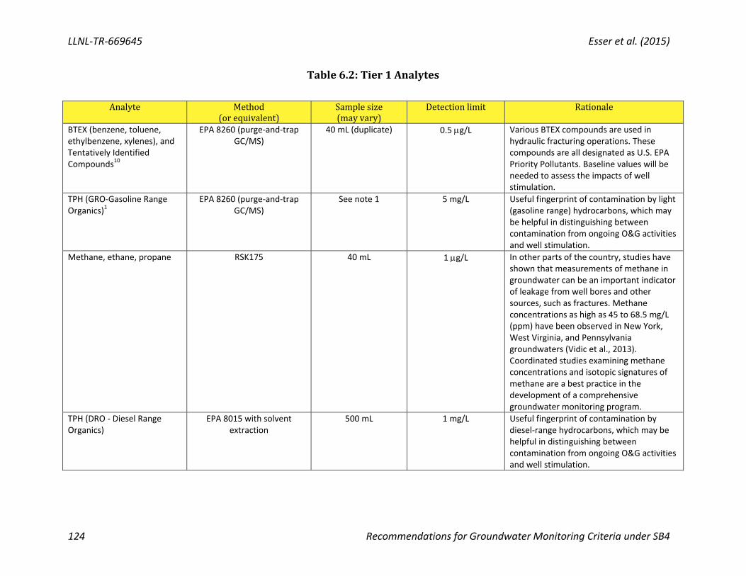
LLNL‐TR‐669645 Esser et al. (2015)
124 Recommendations for Groundwater Monitoring Criteria under SB4
Table6.2:Tier1Analytes
Analyte Method
(orequivalent)Samplesize(mayvary)
Detectionlimit Rationale
BTEX (benzene, toluene, ethylbenzene, xylenes), and Tentatively Identified Compounds10
EPA 8260 (purge‐and‐trap GC/MS)
40 mL (duplicate) 0.5 g/L Various BTEX compounds are used in hydraulic fracturing operations. These compounds are all designated as U.S. EPA Priority Pollutants. Baseline values will be needed to assess the impacts of well stimulation.
TPH (GRO‐Gasoline Range Organics)1
EPA 8260 (purge‐and‐trap GC/MS)
See note 1 5 mg/L Useful fingerprint of contamination by light (gasoline range) hydrocarbons, which may be helpful in distinguishing between contamination from ongoing O&G activities and well stimulation.
Methane, ethane, propane RSK175 40 mL 1 g/L In other parts of the country, studies have shown that measurements of methane in groundwater can be an important indicator of leakage from well bores and other sources, such as fractures. Methane concentrations as high as 45 to 68.5 mg/L (ppm) have been observed in New York, West Virginia, and Pennsylvania groundwaters (Vidic et al., 2013). Coordinated studies examining methane concentrations and isotopic signatures of methane are a best practice in the development of a comprehensive groundwater monitoring program.
TPH (DRO ‐ Diesel Range Organics)
EPA 8015 with solvent extraction
500 mL 1 mg/L Useful fingerprint of contamination by diesel‐range hydrocarbons, which may be helpful in distinguishing between contamination from ongoing O&G activities and well stimulation.

Esser et al. (2015) LLNL‐TR‐669645
Recommendations for Model Groundwater Monitoring Criteria under SB4 125
Analyte Method(orequivalent)
Samplesize(mayvary)
Detectionlimit Rationale
Cations: Na+ (sodium), K+ (potassium), Mg2+ (magnesium), Ca2+ (calcium)
EPA 200.7 (Optical ICP) 200 mL 1 mg/L Measurement of major cations is part of the routine analysis of major constituents in water. Such analytes will be used to detect changes in water quality as well as to deduce contaminant sources. Produced water and wastewater are typically enriched in Na, Ca, and K and their chemical distribution could provide information on the source of groundwater quality degradation.
NH4+ (ammonium) 4500‐NH3‐Nitrogen (Standard
Methods for Water and Wastewater‐EPA‐approved)
100 mL 0.1 mg/L as N High NH4+ concentrations have been
detected in produced waters from both conventional and unconventional oil and gas wastewater in different basins outside California (Harkness et al., 2015). Preliminary data for produced waters from the Central Valley confirm high NH4
+ in produced waters in California.
Anions: Cl‐ (chloride), NO3‐
(nitrate), F‐ (fluoride), SO42‐
(sulfate), Br‐ (bromide)
EPA 300.0 or 353.2 (Ion chromatography)2
40 mL 1 mg/L Measurement of major anions is part of the routine analysis of major constituents in water. Such analytes will be used to detect changes in water quality as well as to deduce contaminant sources. Produced water and wastewater are typically enriched in Cl‐ and distributions of major anions could provide indications of the source of groundwater contamination. In particular, ratios of Br‐/Cl‐ and SO4
2‐/Cl‐ could indicate sources of groundwater quality degradation. Note that these anions would all be analyzed in the same run, so excluding compounds from this list will most likely not result in significant cost savings.

LLNL‐TR‐669645 Esser et al. (2015)
126 Recommendations for Groundwater Monitoring Criteria under SB4
Analyte Method(orequivalent)
Samplesize(mayvary)
Detectionlimit Rationale
Total carbonate (total alkalinity as CaCO3)
SM 2320B (Standard Methods for Water and
Wastewater ‐ EPA‐approved)
100 mL 5 mg/L Potassium carbonate is a compound used in hydraulic fracturing that is used at the 4th greatest mass of all reported chemicals in California (Table 5.3). Naturally occurring alkalinity is also common in produced water and high alkalinity may be present in wastewater from oil‐and‐gas operations in California. Since carbonate species in groundwater may derive from multiple sources, a baseline concentration should be established.
Trace elements (dissolved): Fe (iron), Mn (manganese), Li (lithium), Sr (strontium), B (boron), Ba (barium), I (iodine), U (uranium)
EPA 200.8 (ICP‐MS)3 100 mL 10 ‐ 50 g/L Measurement of trace elements is part of the routine analysis of water quality. Such analytes will be used to detect changes in water quality as well as to deduce contaminant sources. Produced water and oil and gas wastewater are typically enriched in B, Sr, Li, and other trace elements and their chemical distribution and ratios could provide information on groundwater contamination sources. In particular, ratios of B/Cl, Li/Cl, and I/Cl could be indicative of the sources of groundwater quality degradation.

Esser et al. (2015) LLNL‐TR‐669645
Recommendations for Model Groundwater Monitoring Criteria under SB4 127
Analyte Method(orequivalent)
Samplesize(mayvary)
Detectionlimit Rationale
Metals and metalloids (dissolved)4: Ag (silver), As (arsenic), Be (beryllium), Cd (cadmium), [Co] (cobalt], Cr (chromium), Cu (copper), Hg (mercury), [Mo] (molybdenum), Ni (nickel), Pb (lead), Sb (antimony), Se (selenium), Tl (thallium), [V] (vanadium], Zn (zinc)
EPA 200.8 (ICP‐MS) or EPA 200.7 (Optical ICP)3
See note 3 1 ‐ 5 g/L Measurement of metals and metalloids is part of the routine analysis of water quality. Such analytes will be used to detect changes in water quality as well as to deduce contaminant sources. Elevated concentrations of trace elements such as arsenic, boron, molybdenum, chromium, and selenium have been measured in shallow groundwaters in several regions in California. Changes in geochemical conditions in aquifers, such as changes in pH and redox potential associated with oil and gas activities, could alter equilibrium conditions and cause mobilization of metals and metalloids into the groundwater. Most of these analytes are U.S. EPA Priority Pollutants (see note 4). Note that these compounds would all be analyzed in the same sample, so excluding analytes from this list will most likely not result in significant cost savings.

LLNL‐TR‐669645 Esser et al. (2015)
128 Recommendations for Groundwater Monitoring Criteria under SB4
Analyte Method(orequivalent)
Samplesize(mayvary)
Detectionlimit Rationale
Polycyclic aromatic hydrocarbons (16 priority pollutant PAHs)5 and Tentatively Identified Compounds (TIC)10
EPA 625 or EPA 8265 (GC/MS) 1 L (glass)
<10 g/L Naphthalene and possibly other low‐molecular‐weight PAH may be included in well stimulation fluids. Also, surfactants in well stimulation fluids may enhance the aqueous solubility of PAH associated with oil and gas operations. These 16 PAH compounds are all designated as U.S. EPA Priority Pollutants. Baseline values will be needed to assess the impacts of well stimulation. Note that these compounds would all be analyzed in the same run, so excluding analytes from this list will most likely not result in any cost savings. The Tentatively Identified Compounds (TICs) account for knowledge gaps and the reality that not all important analytes can be targeted a priori, and uses mass spectrometry to identify large peaks that were not target analytes.
Dissolved organic carbon (DOC)
SM5310 (Standard Methods for Water and Wastewater ‐
EPA‐approved)
40 mL 0.7 mg/L Bulk parameter useful for indicating high loading of organic compounds. Baseline values will be needed to assess the impacts of well stimulation.
Guar gum sugars (Total Carbohydrate Test)
22.3.1. Total Carbohydrates by Anthrone Reaction
or 22.3.2. Total Carbohydrates
by Phenol Reaction Gerhardt, P., Murray, R. G. E., Wood, W. A., & Krieg, N. R. (1994). Methods for General and Molecular Bacteriology (Vol. 1325). Washington, DC:
American Society for Microbiology.
(or equivalent method)
20 mL 5 mg/L (as glucose)
Guar gum is the most commonly reported hydraulic fracturing compound used in California and is also used at the greatest mass of reported chemicals (Table 5.3). Guar gum is a polysaccharide consisting of galactose and mannose, which can be expected to be at extremely low concentrations in native groundwater, and thus could be a powerful indicator. The recommended analysis will hydrolyze guar gum to its component sugars.

Esser et al. (2015) LLNL‐TR‐669645
Recommendations for Model Groundwater Monitoring Criteria under SB4 129
Analyte Method(orequivalent)
Samplesize(mayvary)
Detectionlimit Rationale
Radionuclides: Ra‐226, Ra‐228, uranium (see note 8) (22 CCR § 64442)
EPA 900.0 ( see note 9) 30 mL Ra‐226 & Ra‐228 combined: 1 pCi/L
Uranium: 1 pCi/L
See note 8
Contaminants associated with oil and gas development wastewaters, including TDS, trace elements, and NORM (Naturally Occurring Radioactive Materials), occur naturally in California groundwater and regional surveys are needed to establish background concentrations in areas of oil and gas development in order to determine how this activity is impacting groundwater.
Total dissolved solids (TDS) See note 6 200 mL 1 mg/L Salt content, measured as TDS, is a critical limiting factor for the quality of groundwater. Beneficial uses of groundwater typically have a TDS threshold above which the water is aesthetically undesirable or will result in impairment. For instance, the taste of water may become unpleasant and agricultural plant growth reduced if TDS levels are above certain thresholds. For these reasons, there are various regulatory limits for water quality based on the total dissolved solids content, some of which are listed in Table 3.1.
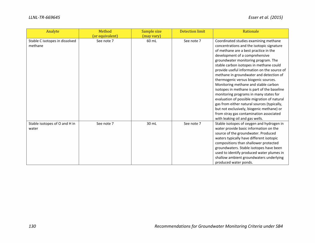
LLNL‐TR‐669645 Esser et al. (2015)
130 Recommendations for Groundwater Monitoring Criteria under SB4
Analyte Method(orequivalent)
Samplesize(mayvary)
Detectionlimit Rationale
Stable C isotopes in dissolved methane
See note 7 60 mL See note 7 Coordinated studies examining methane concentrations and the isotopic signature of methane are a best practice in the development of a comprehensive groundwater monitoring program. The stable carbon isotopes in methane could provide useful information on the source of methane in groundwater and detection of thermogenic versus biogenic sources. Monitoring methane and stable carbon isotopes in methane is part of the baseline monitoring programs in many states for evaluation of possible migration of natural gas from either natural sources (typically, but not exclusively, biogenic methane) or from stray gas contamination associated with leaking oil and gas wells.
Stable isotopes of O and H in water
See note 7 30 mL See note 7 Stable isotopes of oxygen and hydrogen in water provide basic information on the source of the groundwater. Produced waters typically have different isotopic compositions than shallower protected groundwaters. Stable isotopes have been used to identify produced water plumes in shallow ambient groundwaters underlying produced water ponds.
Esser et al. (2015) LLNL‐TR‐669645
Recommendations for Model Groundwater Monitoring Criteria under SB4 131
Footnotes1 BTEXandTPH‐GRO,canberunonthesamesample.2 Bromidemayrequireaspecialrequest;iodidecouldbeanalyzedbyionchromatographybutiodineislistedwithtraceelementsbecausethatanalysiswillbemore
sensitive.3 Traceelementsandmetalscanbeanalyzedinthesamesample.4 Otherthanthethreeelementsinbrackets,thesemetals/metalloidsareUSEPAPriorityPollutants.Thethreeelementsinbracketscanbeanalyzedinthesame
sampleastheothermetals.5 The16PAHinclude:acenaphthene,acenaphthylene,anthracene,benz[a]anthracene,benzo[b]fluoranthene,benzo[k]fluoranthene,benzo[a]pyrene,
benzo[ghi]perylene,chrysene,dibenzo[a,h]anthracene,fluoranthene,fluorene,indeno[1,2,3‐cd]pyrene,naphthalene,phenanthrene,andpyrene.6 TDScanbecalculatedasthesumofcationsandanions.7 ThereisnoEPAstandardmethodforisotopicanalysis,anddetectionlimitsdonotapply.8 Uraniumcanalsobeanalyzedbyinductively‐coupledplasmamassspectrometry(ICPMS).9 AnymethodthatmeetstherequirementsofCaliforniaCodeofRegulations,title22,§64442and64443.10 TentativelyIdentifiedCompounds(TICs)willconsistofthetenlargestnon‐targetpeaksinasamplechromatogram.Thelaboratoryshouldprovidethemass
spectraforthesepeaksandthebestMSlibrarymatches,aswellasanestimatedconcentration(basedonthemostsimilaravailablestandard).DetailedguidanceonhandlingTICsisprovidedbytheU.S.EPA(2014b).
WeacknowledgeLarryChrystal(BabcockLaboratories,Inc.)andStuartButtram(BCLaboratories,Inc.)forassistancewiththistable.

LLNL‐TR‐669645 Esser et al. (2015)
132 Recommendations for Groundwater Monitoring Criteria under SB4
6.2 SummaryofRecommendationsforArea‐SpecificGroundwaterMonitoringCriteria
Groundwater Sampling, Testing, and Monitoring for Hydraulic Fracture or Acid Well Stimulations Where Protected Groundwater is Present.
(a) The purpose of this section is to provide recommendations for the State Water Board to consider for groundwater monitoring model criteria for groundwater sampling, testing, and monitoring related to well stimulation treatment (WST) in areas where protected groundwater exists. Protected groundwater is defined as groundwater with Total Dissolved Solids (TDS) of less than 10,000 mg/L in an aquifer of sufficient volume for beneficial use and for which the Water Board has not concurred on a request for exclusion from groundwater monitoring. These area‐specific groundwater monitoring criteria do not apply to regional groundwater monitoring programs developed by the State Water Board or the Regional Water Board.
(b) The Board should consider the following factors in reviewing requests for exclusion from groundwater monitoring:
(1) The aquifer is not now supplying water for beneficial use (with the exception of industrial activities such as enhanced oil recovery); and
(2) The aquifer cannot now and will not in the future serve as a source of water for beneficial use (with the exception of industrial activities such as enhanced oil recovery) because:
(A) Groundwater is not present or is present in insufficient quantity to supply a single well capable of producing an average, sustained yield of 200 gallons per day;
(B) The aquifer is so contaminated as to be impractical to render the water fit for beneficial use (with the exception of industrial activities such as enhanced oil recovery);
(C) The aquifer is mineral, hydrocarbon or geothermal energy producing and does not now nor is expected in the future to serve as a source of water for beneficial use (with the exception of industrial activities such as enhanced oil recovery); or
(3) The total dissolved solids content of the ground water is more than 10,000 mg/L and it is not reasonably expected to supply water for beneficial use.
(c) An area‐specific groundwater monitoring plan for a single stimulation well or a group of stimulation wells that are closely spaced and part of a single project shall include all of the following:
(1) A map showing the location of all existing groundwater supply wells (public, private domestic, irrigation, and industrial), Class II injection wells, groundwater monitoring wells, and all active and abandoned or inactive oil and gas wells

Esser et al. (2015) LLNL‐TR‐669645
Recommendations for Model Groundwater Monitoring Criteria under SB4 133
(A) within 1 mile of any vertical well(s) to undergo stimulation, or
(B) within 1 mile of the surface projection of the portion of the well to undergo stimulation in directionally drilled horizontal wells.
(2) The estimated well stimulation extent in three dimensions or Axial Dimensional Stimulation Volume (ADSV) is determined to ensure the geologic and hydrologic isolation of the oil and gas formation during and following well stimulation treatment along with supporting data. For determining the need for groundwater monitoring, the ADSV should reflect a “groundwater protective” conservative estimate of the location of the volume stimulated, meaning that the maximum estimated height, length, and depth, incorporating uncertainty in these predictions, should be used
(A) The Operator is required to provide relevant mechanical rock properties, including the stress profile or fracture gradient, the method used to determine them, and any additional data used to estimate ADSV and to demonstrate the geologic and hydrologic isolation of the well stimulation fluids or any fluids from the stimulated target zone during and following stimulation. Fluids are defined in this document to include liquids and gases. For example, in the instance that the ADSV is contained by a stress barrier, the furnished supporting information should specifically include the stress profile or fracture gradient along with the data to support it.
(B) The ADSV should assume a 360 degree radial azimuthal extent in the stratigraphic plane of the reservoir and a vertical extent that is equivalent to the longest predicted dimension (whether vertical or lateral). The Operators may propose a different volume that restricts the azimuthal extent or the vertical extent, but the proposal must be supported by field data, all wells and geologic features excluded by restriction of the azimuth or vertical extent must be identified by location and radial distance from the stimulated well, and the Board retains discretion over how ADSV is defined.
(C) If there are multiple stages, the ADSV is determined for each individual stage.
(D) The operator is responsible for any unintended events that occur during a WST that result in migration of fluids outside the ADSV and negatively impact protected groundwater quality.
(3) A map and cross‐section of the well(s) to undergo stimulation, showing
(A) Well name(s),
(B) The extent, and orientation if applicable, of the planned stimulation on both map and cross‐section, including any uncertainty, and the method and supporting data used to estimate the planned extent,
(C) Depths of the vadose zone and water table
(D) The distribution of groundwater salinity and gas presence and composition in aquifers along the stratigraphic section between the water table and target formations,

LLNL‐TR‐669645 Esser et al. (2015)
134 Recommendations for Groundwater Monitoring Criteria under SB4
(E) Depths of all protected groundwater aquifers, the strata that contain them, and the basis for determining the distribution and quality of the protected groundwaters,
(F) Depths of any aquifers classified as exempt from the Safe Drinking Water Act (SDWA) and depths of any active or inactive Class II injection wells showing their zones of injection.
(G) Depths of low‐permeability zones and the strata that contain them that will function to hydraulically isolate the protected waters or the surface from any fluids injected or produced during or following the WST,
(H) Any wellbore within two times the ADSV of individual stimulation stages, (Wellbores located within the surface projection of the ADSV, but that do not extend deep enough to intersect this volume, can be excluded), and
(I) Any known geologic features within or intersecting five times the ADSV of any stage that have the potential to constitute a leakage pathway, including faults, fractures, joint zones, and changes in hydrostratigraphy that provide substantial permeability.9
(4) Data relevant to the determination of salinity and gas distribution in aquifers along the stratigraphic section between the water table and target formations, including the methods used the acquire the data and the provenance of the data;
(5) A complete description of the well(s) to be stimulated, and any wells within two times the ADSV for any stage, including the following information for the well to be stimulated and, when available, for any wells with two times the ADSV for any stage,
(A) Any available geophysical logs characterizing properties (porosity, moduli, saturating fluid characterization, etc.) of the target formation and underburden/overburden, such as Spontaneous Potential, Resistivity, Caliper, and any porosity logs (e.g. Formation Density/Neutron or Acoustic Velocity logs, etc);
(A) Any information (such as Driller’s Reports or Mud Logs) relevant to assessment of borehole instability, “washouts”, or fluid loss during drilling or well installation and completion.
(B) Casing diagrams and leakage risk assessment, including the following:
(i) Sizes and weights of casing;
(ii) Depths of shoes, stubs, and liner tops;
(iii) Depths of perforation intervals, water shutoff holes, cement port, cavity shots, cuts, casing damage, and top of junk or fish left in well;
(iv) Diameter and depth of borehole;
(v) Cement plugs inside casings, including top and bottom of cement plug, with indication of method of determining;
(vi) Cement fill behind casings, including top and bottom of cement fill, with

Esser et al. (2015) LLNL‐TR‐669645
Recommendations for Model Groundwater Monitoring Criteria under SB4 135
indication of method of determining;
(vii) Type and weight (density) of fluid between cement plugs;
(viii) Depths and names of the formations, zones, and markers penetrated by the well, including the top and bottom of the zone where well stimulation treatment will occur;
(ix) All steps of cement yield and cement calculations performed;
(x) All information used to calculate the cement slurry (volume, density, yield), including but not limited to, cement type and additives, for each cement job completed in each well;
(xi) All of the information listed in this paragraph that is available for all previous redrilled or sidetracked well bores.
(xii) Wellbore path giving both inclination and azimuth for directionally drilled wells
(xiii) Based on the above information, the State will conduct an assessment of the risk of leakage to protected groundwater along the well to be stimulated and any wells within two times the ADSV of all the stages. As a result of this review, the State may require additional information from the Operator in the form of cement evaluation logging or pressure testing to demonstrate adequate well integrity prior to approving the WST permit.
(6) For any geologic features within or intersecting five times the ADSV of any stage that have the potential to constitute a leakage pathway, including faults, fractures, and changes in hydrostratigraphy, the operator is required to provide:
(A) Any data or evaluation that has bearing on whether the geologic feature may act as a vertical conduit for migration of injected fluids, released fluids or displaced formation fluids; and
(i) An assessment of the risk that the well stimulation treatment will communicate with the geologic feature, and if so, will communicate with protected groundwater via the feature.
(ii) The State will review the information provided by the Operator and may require additional information to assess the risk that injected fluids could migrate upward along the geologic feature prior to approving the WST permit.
(7) Map(s) and cross‐section(s) showing locations of groundwater wells (new and existing monitoring wells and supply wells), including those to be sampled for groundwater monitoring. The following information, when known and available, should be shown:
(A) Maps should extend at least 2 miles from the stimulated well in a down gradient direction and one half mile in an up gradient direction. The map should contain all surface features normally displayed on a USGS topography map, be clearly readable, and clearly show the well to be stimulated, all groundwater monitoring and water‐supply wells, and Class II injection wells, all

LLNL‐TR‐669645 Esser et al. (2015)
136 Recommendations for Groundwater Monitoring Criteria under SB4
oil and gas wells, any such wells that have been previously stimulated, and any active or inactive oilfield wastewater disposal pits or surface impoundments;
(B) Potentiometric surface map displaying each well specific to the aquifer used to generate the map and, based on this surface and any other information indicated on the map, arrows indicating the general groundwater flow direction in the vicinity of the well;
(C) Groundwater elevation measurements used to generate the groundwater elevation contour map(s) should be measured as contemporaneously as possible (within 30 days);
(D) All water‐supply wells should be clearly marked on the map, including wells sampled in the State Water Board Groundwater Ambient Monitoring and Assessment (GAMA) project. For active water‐supply wells, the operator should document whether the water level that appears on the groundwater elevation map was measured during pumping or non‐pumping conditions;
(E) Active or inactive Class II injection wells showing their zones of injection should be clearly marked on the map and cross‐section;
(F) Any unlined sumps used to discharge oilfield waste fluids should be clearly shown on the map;
(G) The number of wells that have been stimulated within one half mile of the proposed stimulated well and their names and locations on the map;
(H) The operator is required to provide, at least, one cross‐section that includes the stimulated well, an up gradient “background” groundwater monitoring well and one or more down gradient monitoring wells and any injection wells including the depths of any screens or perforations and any annular materials. The cross‐section should clearly display to the extent known the hydrostratigraphy (including water levels), identifying all protected aquifers, the base of protected water, any exempt aquifers, and should include any geophysical logs or groundwater quality samples and methodology used to determine the base of protected water;
(I) The cross‐section should extend from the surface to a depth of at least 150 meters (500 ft) below the protected water; and
(J) For each protected aquifer, indicate any available hydraulic conductivity data in meters per second (m/s) and the source of the data (e.g., hydraulic test).
(8) Additionally, for all new and existing groundwater wells that will be used for monitoring, the operator will submit groundwater well completion reports including construction details and any lithologic information collected during well installation, to demonstrate that their construction details meet California Well Standards contained in Department of Water Resources Bulletin 74‐81 as supplemented by Department of Water Resources Bulletin 74‐90.

Esser et al. (2015) LLNL‐TR‐669645
Recommendations for Model Groundwater Monitoring Criteria under SB4 137
(9) A list of chemical additives and tracers anticipated to be used in the well stimulation, including
(A) A complete list of the names, Chemical Abstracts Service Registry Numbers (CASRN), and estimated concentrations, in percent by mass, of each and every chemical constituent of the well stimulation fluids anticipated to be used in the treatment (if a CASRN does not exist for a chemical constituent, another unique identifier may be used, if available;
(B) Whether it is anticipated that radiological components or tracers will be injected during the well stimulation treatment, and a list of those radiological components and tracers that will be used;
(10) A contingency plan for reporting information in the event of a well failure, or any other unintended event that has the potential to affect groundwater quality, such as the detection of an induced fracture beyond the ADSV or into protected waters. A “well failure” means any instance where the stimulation did not proceed as intended, including a failure of the stimulated well or any nearby well failure, resulting in a subsurface leak of gas or water with excessive salt or other dissolved deleterious constituents that might extend to protected groundwater. The contingency plan shall, at a minimum, require the well operator to submit the following information to the Division, the State Water Board, and the appropriate Regional Water Quality Control Board within 48 hours of discovery of a well failure or other unintended event that may have resulted in the migration of fluids introduced during the stimulation or the production of liquids or gases from any zone between the stimulation target zone and the protected water, to anywhere outside the ADSV:
(A) A description of the activities and all real‐time monitoring data that was collected during the stimulation, including treatment and bottom hole pressures, slurry injection rate, bottom hole proppant and slurry concentrations, and the method for estimating fluid loss and the sensitivity of this measurement. In the event of a stimulation failure, the operator will identify the specific data that indicated a well failure or unintended event;
(B) Depth interval(s) of the well failure or unintended event and evidence used to estimate the depth of the well failure or unintended event. The operator is encouraged to use best available methods, including the use of tracers if necessary, to identify the depth of well failure;
(C) Chemical composition of all well stimulation treatment fluids and proppants introduced into the stimulated well and any stimulation target zone(s), including any tracers introduced to determine the depth of well failure;
(D) Chemical composition of fluids produced before, during or and after the well failure, or unintended event;
(E) An estimate of the volume and composition of fluid lost during well failure, or unintended event and the basis for the volume estimation; and

LLNL‐TR‐669645 Esser et al. (2015)
138 Recommendations for Groundwater Monitoring Criteria under SB4
(F) Real‐time monitoring data.
(G) In response to the potential release, the operator and the appropriate Regional Water Quality Control Board will use the information provided as required above to develop a groundwater investigation and corrective action plan, including groundwater samples to be collected from existing groundwater monitoring wells, installation of additional groundwater monitoring wells, and specialty analyses to be conducted based on any stimulation tracers and end‐member chemistry (e.g., hydrofracture fluids, “flowback,” and produced reservoir fluids).
( d ) Area‐specific groundwater monitoring, including the location and design of monitoring wells described in the groundwater monitoring plan in accord with provisions (b) (6), should be designed for detection of protected water impacts by the WST and characterization of “baseline” water quality in protected groundwaters overlying or underlying WST operations.
(1) An area‐specific groundwater monitoring plan will be required when protected groundwater is either penetrated by the stimulated well or is present at any depth within 0.5 mile of the stimulated well.
(2) A regional groundwater monitoring well will meet the requirement for a groundwater monitoring well in an area‐specific groundwater monitoring plan when protected groundwater is present at any depth within 0.5 mile of the stimulated well and:
(A) No wellbores are present within 2x ADSV of any stage; and/or no potentially transmissive features, such as faults, are present within 5xADSV of any stage, and
(B) Regional groundwater monitoring well(s) screened at the appropriate depth(s) are present within 1 mile of the stimulated well.
(3) Aquifers that are mineral, hydrocarbon or geothermal energy producing constitute a special case under area‐specific groundwater monitoring.
(A) Water with <10,000 mg/L TDS produced from a stimulated well is required to be monitored on the same semi‐annual schedule and for the same analytes as other protected groundwaters under the area‐specific plan. Samples for this monitoring may be taken from the water produced from the specific well or from any downstream location where this water may be commingled with water produced from other wells. Sampling must continue at this location on the schedule specified until concentrations stabilize.
(B) Additional monitoring locations in the mineral, hydrocarbon or geothermal energy producing aquifer being used for non‐industrial beneficial use are not required under the area‐specific groundwater monitoring plan.
(4) Under certain circumstances, the Board will not approve a groundwater monitoring plan, or will require additional measures to prevent contamination of protected groundwater:

Esser et al. (2015) LLNL‐TR‐669645
Recommendations for Model Groundwater Monitoring Criteria under SB4 139
(A) If two times the longest dimension of the ADSV of any stage extends to within 100 feet of the protected groundwater zone, then the Water Board reserves the right to not allow the well stimulation treatment to proceed by not approving a groundwater monitoring plan.
(B) If produced water from the target zone for the well stimulation is being used or proposed for non‐industrial activity beneficial use (e.g. for domestic or municipal water supply or for agricultural irrigation and not for enhanced oil recovery), then the State reserves the right to deny the well stimulation treatment or to require a plan for treatment of the produced water prior to beneficial use that will remove chemicals present due to well stimulation (including stimulation fluid constituents, their degradation products, and natural constituents mobilized by the stimulation). This restriction does not apply to the use of produced waters within a subsurface zone that the Board has determined does not require protection, e.g. for enhanced oil recovery.
(C) If produced water from zones overlying the proposed target zone is being used or proposed for beneficial use outside of the oil and gas field (e.g. for irrigation), then a plan is required for monitoring of the produced water prior to beneficial use.
(5) Sufficient monitoring wells should be included in the monitoring plan to adequately characterize and protect potentially impacted aquifers. The number of new and existing groundwater wells required for groundwater monitoring, and the frequency and length of monitoring will vary depending on the Site Conceptual Model, and should take into account site specific factors such as the number, spacing, and location and depth of the stimulated well(s), the distance from the stimulated well to the groundwater monitoring well(s), hydraulic gradient magnitude and direction, and the average hydraulic conductivity of the protected aquifers.
(A) A groundwater monitoring location may consist of a single or multiple groundwater monitoring wells depending on the thickness and number of protected aquifers present. When multiple protected aquifers to be monitored are present, each aquifer at a given location must be monitored separately by appropriate means. Options for appropriate monitoring strategies include three approaches, with each monitoring location targeting one or more hydrostratigraphic units using separate well screens or other types of monitoring technologies:
a. A cluster of conventional monitoring wells, each well in a separate borehole screened in a different hydrostratigraphic unit;
b. A depth‐discrete multilevel monitoring system installed in a cased well or stable uncased borehole capable of monitoring one or more hydrostratigraphic units; or
c. Nested wells in a single borehole, each individual well with a screen in a different hydrostratigraphic unit and with seals between each well

LLNL‐TR‐669645 Esser et al. (2015)
140 Recommendations for Groundwater Monitoring Criteria under SB4
screen and the other wells in the borehole. Nested wells should be used with caution because they have more uncertainty than the other approaches in the integrity of the seals between individual screens.
(B) In general, the number of aquifer monitoring locations will increase as the number of stimulations in an area increases, but the proportion of monitor locations to stimulated wells will decline. For instance, three monitoring locations (one upgradient and two downgradient) may be required for each monitored groundwater aquifer when a well stimulation is far removed from other stimulations. On the other hand, for ten stimulations clustered in a small area, only six monitoring locations for each monitored groundwater aquifer might be necessary to meet the proximity requirements.
(C) A single groundwater monitoring plan may be developed for a project consisting of more than one well stimulation.
(D) Operators may submit an alternative plan with specifications that differ from the provisions that follow and that takes into account site‐specific conditions, but must provide documentation that the alternative plan is based on a Site Conceptual Model and achieves at least the same level of groundwater protection as a plan with specifications that comply with the provisions that follow.
(6) Groundwater monitoring plans will be approved for stimulated well locations that are either not in close proximity to existing wells or geologic features or that are in close proximity to existing wells that have been sealed or abandoned in a manner protective of protected groundwater aquifers or to geologic features not known to be transmissive.
(A) For existing wells, close proximity is defined as within 2xADSV of the stimulated well.
(B) For geologic features, close proximity is defined as within 5xADSV of the stimulated well.
(C) Demonstrating that a well has been sealed or abandoned in manner protective of protected groundwater aquifers requires that the operator
i. Document that abandoned wells in close proximity were abandoned properly to prevent degradation of protected groundwater quality;
ii. Document that for active or idle wells in close proximity,
1. The annular space of the production casing is sealed from the top of the stimulated well interval up to at least 100 feet into a regional seal more than 2xADSV above the top of the target zone or 500 feet, whichever is longer; and
2. The annular space of production or intermediate casing is sealed from a regional aquitard below protected groundwater to at least 100 ft into the next larger diameter casing; and

Esser et al. (2015) LLNL‐TR‐669645
Recommendations for Model Groundwater Monitoring Criteria under SB4 141
iii. Provide evidence for active or idle wells in close proximity that the mechanical integrity of the annular cement seals will prevent unintended migration of fluids that could degrade protected groundwater quality
(7) Groundwater monitoring should be based on risk to the groundwater resource and on the quality of the groundwater resource being protected. The requirements below are contingent on the operator demonstrating that there has been no significant loss of injected fluid outside of the target zone during the stimulation event.
(A) For all stimulated wells (with one exception), monitoring is required for at least two aquifers:
i. A freshwater (0‐3,000 mg/L) aquifer with the highest quality water (i.e., the lowest TDS) at the location, and
ii. A protected groundwater (3‐10,000 mg/L) aquifer near the stimulated zone, which will commonly be an aquifer near the base of the protected groundwater zone.
iii. For exploratory stimulated wells with less than 4 previously stimulated wells within ½ mile radius and with no existing wells within 2xADSV or geologic features within 5xADSV, only monitoring of the freshwater aquifer is required.
(B) For stimulated wells in densely drilled fields (i.e., stimulated wells with in excess of 50 previously stimulated wells within ½ mile), monitoring is also required of an aquifer near the base of freshwater (0‐3,000 mg/L TDS).
(8) Approval of groundwater monitoring plan for stimulated well locations in close proximity to wells not demonstrated to be abandoned or sealed in manner protective of protected groundwater aquifers will require additional review and may not be granted.
(A) Additional review will include more stringent assessment of
i. The construction and sealing of existing wells in close proximity (including documentation of cemented and uncemented intervals);
ii. The transmissivity of geologic features in close proximity;
iii. The site hydrogeology (including the presence or absence of regional aquitards and seals);
iv. The current and future use of protected groundwater aquifers
(B) On the basis of additional review, the Water Board may
i. Deny approval of a groundwater monitoring plan and thereby prevent the well stimulation from proceeding;
ii. Approve a groundwater monitoring plan, but require additional monitoring, including one or both of the following actions.
1. Monitoring of additional aquifers determined to be at risk.
2. Installation of additional monitoring locations for each aquifer

LLNL‐TR‐669645 Esser et al. (2015)
142 Recommendations for Groundwater Monitoring Criteria under SB4
monitored.
(9) All groundwater monitoring wells should be completed with limited screen lengths, preferably less than less than 50 feet. The length of screen should be commensurate with potential pathways for contamination and 50 feet may be excessive.
(10) The operator is required to locate groundwater monitoring wells within reasonable proximity, within 0.5 mile, in a down gradient direction of the oil or gas well(s) undergoing well stimulation treatment.
(11) Any active water‐supply wells within 1 mile of the stimulated well in a down gradient direction should be protected by installing a guard well or guard wells between the stimulated well and the water‐supply well along a reasonable groundwater flow pathway for the active water supply well. If the water‐supply well is screened across multiple protected aquifers, then each protected aquifer should be monitored separately.
(12) To the extent possible, the operator is required to continuously monitor groundwater in guard wells for changes in water level and electrical conductivity (e.g., specific conductance) using in‐situ sensors with data loggers.
(13) If any groundwater wells identified in accordance with subsection (b)(3) are not to be used for groundwater monitoring, a justification for their exclusion shall be included in the groundwater monitoring plan.
(14) Area‐specific groundwater monitoring plans that assert the absence of protected water as the basis for not conducting groundwater monitoring require the Water Board’s written concurrence with the operator’s determination of the absence of protected water.
( e ) If new groundwater wells are used for area‐specific groundwater monitoring, they shall be constructed and properly developed in accordance with any applicable local well ordinances.
If there are no applicable local well ordinances, they shall be constructed in accordance with the California Well Standards contained in Department of Water Resources Bulletin 74‐81 as supplemented by Department of Water Resources Bulletin 74‐90.
( f ) For area‐specific groundwater monitoring, the operator should sample the groundwater monitoring wells frequently enough to detect changes in water quality.
(1) The operator shall sample the groundwater monitoring wells before well stimulation commences in order to establish baseline water quality. Following the stimulation, the area‐specific groundwater monitoring wells will be placed on a semi‐annual monitoring schedule.
(2) The quarter selected for semi‐annual sampling should alternate each year. For example, the 1st year, the operator will collect samples during the 1st and 3rd quarter; the following year, samples will be collected during the 2nd and 4th quarters.
(g) For all groundwater sampling, testing, and monitoring conducted pursuant to this Article,
(1) Groundwater level and field parameters including pH, temperature, electrical

Esser et al. (2015) LLNL‐TR‐669645
Recommendations for Model Groundwater Monitoring Criteria under SB4 143
conductivity, dissolved oxygen, hydrogen sulfide, and oxidation‐reduction potential shall be measured and recorded before and after sample collection.
(2) For all groundwater sampling, testing, and monitoring conducted pursuant to this Article, groundwater samples shall be analyzed using current applicable EPA‐approved analytical methods for water, if available, for all of the following:
(A) total dissolved solids;
(B) major and minor cations, including sodium, potassium, magnesium, calcium, and ammonium;
(C) major and minor anions, including nitrate, chloride, fluoride, sulfate, bromide, iodide, and total inorganic carbonate (bicarbonate + carbonate);
(D) trace elements, including iron, manganese, lithium, strontium, barium, and boron;
(E) all metals and metalloids listed in California Code of Regulations, title 22, section 66261.24, subdivision (a)(2)(A), including arsenic, barium, cadmium, chromium, lead mercury, and selenium (excluded from the Title 22 list are asbestos and fluoride salts);
(F) radionuclides listed under California Code of Regulations, title 22, Table 64442 (includes Ra‐226, Ra‐228, and uranium);
(G) methane, ethane, propane;
(H) dissolved organic carbon (DOC);
(I) BTEX (benzene, toluene, ethylbenzene, and xylenes) and Tentatively Identified Compounds (TICs);
(J) total petroleum hydrocarbons for crude oil and gasoline and diesel ranges;
(K) PAH (polynuclear aromatic hydrocarbons) including the 16 priority pollutant PAHs (acenaphthene, acenaphthylene, anthracene, benz[a]anthracene, benzo[b]fluoranthene, benzo[k]fluoranthene, benzo[a]pyrene, benzo[ghi]perylene, chrysene, dibenzo[a,h]anthracene, fluoranthene, fluorene, indeno[1,2,3‐cd]pyrene, naphthalene, phenanthrene, and pyrene), and Tentatively Identified Compounds (TICs);
(L) stable carbon isotopes in dissolved methane (if present);
(M) stable isotopes of oxygen and hydrogen in water;
(N) guar gum sugars (if guar gum is used in the well stimulation);
(O) At least two analytes selected by the applicant, with the review and agreement of the Water Board. The analytes chosen will be well stimulation chemical additives or their degradation products. One constituent will be chosen based on large soluble mass used during well stimulation; the other constituent will

LLNL‐TR‐669645 Esser et al. (2015)
144 Recommendations for Groundwater Monitoring Criteria under SB4
be chosen based on high persistence in the subsurface. Each constituent should be in the 90th percentile or above of all constituents for the particular property and should also rank as highly as possible in the other property. Availability of analytical methods should also be considered. For instance, if there are several constituents of high persistence, then the constituent with combination of greatest mass and persistence should be monitored, presuming there is an accepted analytical method for doing so.
(3) If concentrations of the analytes listed above (with the exception of Tentatively Identified Compounds) change between sampling events in a manner consistent with impact from a stimulation as determined using the method specified in (h)(4), then analysis shall be conducted for the following compounds if they are used in well stimulation
(A) cationic, anionic, and nonionic surfactants used during well stimulation
(B) alcohols and glycols used during well stimulation
(C) biocides used during well stimulation, including any of the following compounds and their known harmful or persistent degradation products:
(i) glutaraldehyde;
(ii) DBNPA (2,2‐dibromo‐3‐nitrilopropionamide) and its degradation products dibromoacetonitrile, dibromoacetic acid, and dibromoacetamide;
(iii) isothiazolinones (e.g., 2‐methyl‐3‐isothiazolinone, 5‐chloro‐2‐methyl‐3‐isothiazolinone);
(D) tracers used during well stimulation
(4) If any of the analytes from the second tier of analyses above in (f)(3) are detected, then the operator will work with the Water Board to develop further analyses based on the chemical additives used in the well stimulations being monitored.
(h) For all groundwater sampling, testing, and monitoring conducted pursuant to this Article, groundwater sampling shall be done in accordance with all of the following:
(1) All groundwater sampling is to be performed by a qualified person.
(A) A qualified person is any person with the knowledge and training in proper sampling methods, chain of custody, and quality assurance/quality control protocols.
(B) Any person conducting groundwater sampling, other than personnel from an approved laboratory, shall consult with the laboratory to ensure that the sampler understands and follows the proper sampling collection procedures and protocols.
(2) All procedures to sample groundwater monitoring wells shall be consistent with U.S. Environmental Protection Agency (US EPA) Groundwater Sampling Guidelines for Superfund and RCRA Project Managers (May 2002). All procedures to sample

Esser et al. (2015) LLNL‐TR‐669645
Recommendations for Model Groundwater Monitoring Criteria under SB4 145
groundwater supply wells shall be consistent with US EPA Science and Ecosystem Support Division Operating Procedure for Groundwater Sampling (March 2013), including pre‐sampling purge methods and purge volumes consistent with Detection Monitoring protocol.
(3) All analytical testing shall be performed by a laboratory that is certified by the California Department of Public Health environmental laboratory accreditation program (ELAP) or a laboratory approved by the Water Board.
(i) All groundwater monitoring data collected in accordance with an area‐specific groundwater monitoring plan, including all chemical, hydraulic and any sensor data, shall be compiled in a groundwater monitoring report, and submitted to the State Water Board.
(1) Semi‐annual groundwater monitoring reports shall include, at a minimum:
(A) Site map with locations of wells used for groundwater monitoring, any water‐supply wells, including wells participating in the GAMA project, and all oil and gas wells.
(B) Table(s) of analytical results, with both recent and historical data in chronological order and tabulated by well number.
(C) Groundwater elevation map(s) for each protected aquifer and at least, one cross‐section displaying groundwater analytical results.
(D) Description of field procedures, including well installation or selection, and groundwater sampling.
(E) Copies of analytical laboratory reports, including quality assurance/quality control procedures and analytical test methods.
(F) Changes, if any, to the scope of work, and rationale for the changes.
(G) Decontamination procedures.
(H) Waste management and disposal procedures, including associated documentation.
(2) Data collected prior to commencement of the well stimulation treatment and public disclosures required under Chapter 4, Subchapter 2, Article 1 Provision 1788 shall be submitted in first semi‐annual groundwater monitoring report
(3) All groundwater quality data and groundwater monitoring reports shall be submitted to the State Water Board in an electronic format that follows the guidelines detailed in California Code of Regulations, title 23, division 3, chapter 30 (commencing with section 3890).
(4) Groundwater monitoring data will be used to first establish baseline conditions of monitored constituents in protected groundwater, and thereafter to determine whether any significant groundwater quality impacts have occurred relative to a baseline.
(A) Multiple years of semi‐annual sampling before or after the stimulation are
LLNL‐TR‐669645 Esser et al. (2015)
146 Recommendations for Groundwater Monitoring Criteria under SB4
recommended for establishment of a baseline. If possible, baseline data collection should start as far as possible in advance of the stimulation. For existing wells, water quality data generated for other programs can be used to establish baseline for constituents monitored by those programs. For new wells or for wells without preexisting water quality data, samples collected immediately before the stimulation and collected semi‐annually for up to three years after the stimulation can be used to establish a baseline. Three years of semi‐annual sampling is recommended if groundwater transport is sufficiently slow.
(B) The operator will also propose the use of a method or methods that will be used after baseline data collection is complete to identify evidence of changes in constituent concentrations that might indicate impact to the groundwater from the stimulation. A recommended method is the 1 of 3 version of the prediction limit with retesting strategy in Chapter 19 of USEPA (2009). The operator may propose and justify an alternate method or methods to identify changes in groundwater that might indicate impact to groundwater from the stimulation. Data from wells upgradient of the stimulation may be used to help distinguish water quality impacts due to the stimulation from impacts due to other causes.
(C) The State will evaluate data and statistical test results to determine whether any impacts have occurred, additional monitoring is necessary, or a corrective action is required. Statistical evidence of a change in constituent concentrations is not, by itself, evidence of an impact from the stimulation.
USEPA (2009) Statistical Analysis of Groundwater Monitoring Data at RCRA Facilities:
Unified Guidance., U. S. Environmental Protection Agency EPA 530/R‐09‐007. http://www.epa.gov/solidwaste/hazard/correctiveaction/resources/guidance/sitechar/gwstats/index.htm.
NOTE: Authority cited: Section 3013, 3160, and 3161, Public Resources Code. Reference: Section 3106, 3160, and 3161, Public Resources Code; Section 10783, Water Code.
Esser et al. (2015) LLNL‐TR‐669645
Recommendations for Model Groundwater Monitoring Criteria under SB4 147
7 RECOMMENDATIONSFORREGIONALGROUNDWATERMONITORINGMODELCRITERIA
7.1 GoalsoftheRegionalGroundwaterMonitoringProgram Defining the goals of the regional groundwater monitoring program (RGMP) is essential to program design and implementation. We recommend that the program be designed to identify potential impacts of all oil and gas activities in the State, including well stimulation, underground injection and wastewater disposal. A primary goal of the State’s regulation of the oil and gas industry has been to assure zonal isolation through stringent well construction standards. An important goal of the RGMP is to demonstrate the extent to which protected groundwaters have been hydraulically isolated from oil and gas‐related produced or injected fluids. How to best design and implement a monitoring plan to identify impacts or demonstrate isolation is not clear – California leads the nation in requiring systematic monitoring of well stimulation. An important aspect of the program will be developing new approaches to monitoring and then testing and refining these approaches over time. 7.1.1 The primary goal of the Regional Groundwater Monitoring Program (RGMP) should be
to be to monitor the impact of oil and gas activities on protected groundwater resources in the State. The primary goal of the Regional Groundwater Monitoring Program (RGMP) is to monitor the impact of oil and gas development on the State’s protected groundwater resources in groundwater basins containing one or more oil and gas fields, produced water ponds, or produced water injection wells. In general, a regional groundwater monitoring plan will encompass a single oil and gas field and protected groundwater within and downgradient from that field. Current hydrological and water quality conditions need to be sufficiently documented and well understood both to guide regulatory policy and to provide direction for future pilot studies. Given the lack of available models for such an effort, the program will need to develop new approaches to regional monitoring with clear objectives and with clear requirements or guidance for the development of individual groundwater monitoring plans. LLNL and its experts concur that the focus of the RGMP should be on the overall impact of oil and gas development in general, rather than on well stimulation alone, with initial prioritization on fields where well stimulation is currently being practiced. Given our current understanding of potential impacts, it will be challenging to separate out impacts from new well stimulations from legacy impacts, including the injection of oilfield wastewaters as part of the Underground Injection Control (UIC) program and the discharge of oil field wastewater to surface pits, particularly at the regional scale.

LLNL‐TR‐669645 Esser et al. (2015)
148 Recommendations for Groundwater Monitoring Criteria under SB4
The primary pathways by which oil and gas development can impact groundwater quality – wastewater disposal through underground injection or discharge to surface pits, surface spills of chemicals and waste water, and transmission of chemicals into protected groundwater as a result of well integrity failures – are not unique to Well Stimulation Treatment (WST). In addition, the impact of WST is not always distinguishable from the impact of other oil and gas operations using available techniques and given the current state of knowledge. For these reasons, the initial focus of the RGMP should be on monitoring the impact of all oil and gas development on protected groundwater resources.
7.1.2 The RGMP should develop regional‐scale conceptual models for protected
groundwaters within and adjacent to oil and gas fields.
Inherent in the development of a regional‐scale groundwater monitoring plan is the establishment of a robust hydrogeologic conceptual model that integrates inter‐disciplinary data, including geology, hydraulics, geophysics and geochemistry. A regional‐scale hydrogeologic conceptual model should clearly define the three‐dimensional, spatial distribution of protected groundwater resources, the hydrostratigraphy that contains this groundwater resource, and the strata that hydraulically separate these groundwater resources from hydrocarbon‐bearing WST target zones. It will be used to determine the optimal lateral and vertical distribution of monitoring points and provide a technical basis for interpreting groundwater monitoring data and design remedial actions in the event of a WST failure that impacts protected groundwater. Additionally, regional‐scale models can be used to calibrate numerical flow and transport models that are needed for decision‐making, including predicting contaminant transport from stimulated wells and fields to downgradient aquifers or water supply well receptors under unstressed and stressed hydraulic conditions. Each regional‐scale conceptual model is likely to be limited initially by significant data gaps and uncertainty that can be reduced and improved with time by the collection and analysis of monitoring data. As model uncertainties are reduced, the regional model will better serve the needs of risk assessment, groundwater management, and corrective actions. The development of these models will require considerable effort by skilled staff capable of inter‐disciplinary data analysis and a clear understanding of regional‐scale groundwater flow and transport processes.
7.1.3 The RGMP should establish monitoring networks to detect transport of fluids from
hydrocarbon producing zones to protected groundwater aquifers that is related to oil and gas development.
The RGMP should (a) document the occurrence or absence of fluid (gas or liquid) transport from hydrocarbon‐producing zones to protected groundwater aquifers, b) characterize pathways and assess the risk of such transport, and c) establish monitoring networks to provide early warning of transport in high risk zones.
Esser et al. (2015) LLNL‐TR‐669645
Recommendations for Model Groundwater Monitoring Criteria under SB4 149
This objective will require mapping out the extent and location of protected groundwater resources near oil and gas fields in three dimensions, and carrying out field‐specific regional assessments to determine if fluids have been or at risk of being transported out of producing zones. These assessments will involve both 1) monitoring of protected groundwaters and characterization of formation fluids, injected fluids, and produced waters followed by geochemical modeling of the collected data to establish baseline, develop geochemical and isotopic signatures for different source waters, and detect impact, and 2) focused field studies using intensive groundwater monitoring, geophysical monitoring, and geochemical, hydrological, geological and geophysical tools and data to identify transport mechanisms and to develop conceptual models linking hydrocarbon producing zones and protected groundwater. These assessments should consider fluids associated with well stimulation, enhanced recovery, and waste injection, and look for evidence of impact of protected groundwater by oilfield brines and gases
7.1.4 The RGMP should characterize risks to and impacts on groundwater resources from
discharge of oil and gas wastewater to surface ponds
The Water Board should characterize the effect of legacy and currently regulated surface activities, including ponds, pits, sumps and spills. Near‐surface contamination by any fluids associated with oil and gas development poses the greatest risk to shallow aquifers currently being used or potentially in the future to be used for beneficial uses such as drinking water and irrigation. The Regional Water Boards currently regulate surface activities and commonly require the operators to conduct site‐specific studies. The RGMP should leverage and complement that work. A goal of the second component then would be to 1) thoroughly characterize the chemical composition and geochemical signature of oil and gas development wastewaters discharged to surface ponds, including the presence of well stimulation and enhanced oil recovery chemical additives; and 2) characterize risks to shallow water users from constituents associated with oil and gas development. The GAMA Program study design applied to an area with a history of surface activities would be an appropriate approach. This component would require that the geochemical end‐member water quality library developed in the transport component include samples of formation water and groundwater under sumps from the study area.
7.1.5 The RGMP should assess the potential risk of well integrity failures and inadequate seals to protected groundwater quality statewide.
The third component of the regional monitoring program is to assess the potential risks to groundwater quality from well bore integrity and inadequate seals. A recent US EPA review of California’s UIC program noted that the cement plugs intended to prevent fluid flow across formation boundaries were not always protective of groundwater

LLNL‐TR‐669645 Esser et al. (2015)
150 Recommendations for Groundwater Monitoring Criteria under SB4
quality. In addition, little is known about how well age, standards of construction, material degradation, improper abandonment, and external forces such as subsidence due to groundwater pumping may correspond to groundwater quality degradation. Investigation of well integrity should follow development of regional conceptual models to ensure that wells have been identified as a transport pathway for a particular region and that enough robust information is available to differentiate between well integrity and other pathways. This component is further complicated by the lack of accurate records documenting the location and construction details for wells of all types (e.g., private wells, deep groundwater monitor or supply wells, legacy oil and gas wells, etc.) that could act as vertical conduits for injected and/or produced fluids in the event of a well integrity failure, are lacking.
7.2 TheProtectedGroundwaterResource A first step in the design and implementation of groundwater quality monitoring is defining the protected resource. We recommend protecting and characterizing the distribution of groundwater with total dissolved solids (TDS) of less than 10,000 mg/L. 7.2.1 The RGMP should monitor groundwater with less than 10,000 mg/L total dissolved
solids (TDS) in aquifers that contain a sufficient quantity of water for beneficial use and that are in groundwater basins containing oil and gas fields. We recommend defining protected groundwater as all groundwater with less than 10,000 mg/L TDS in an aquifer that contains a sufficient quantity of water for beneficial use and that is not excluded from groundwater monitoring by a written concurrence from the Water Board. The ongoing drought in California requires that all waters with the potential for beneficial use in California be protected, and current water purification methods (e.g. reverse osmosis) allow waters greater than 10,000 mg/L TDS to be readily purified to drinking water standards. The RGMP should also include data and monitoring of exempted aquifers and groundwaters with TDS values greater than 10,000 mg/L when such waters represent transport and contaminant pathways and establish geochemical end‐members for source attribution.
7.2.2 The State should implement a program to systematically determine the spatial and vertical distribution of all fresh groundwater (< 3,000 mg/L TDS) and protected groundwater (< 10,000 mg/L) in basins containing oil & gas fields throughout the State. The locations and depths of groundwater in California with TDS values between 3,000 and 10,000 mg/L are not well known, and substantial effort will be needed to identify them. Some data are available in the form of oil and gas field summaries, existing maps
Esser et al. (2015) LLNL‐TR‐669645
Recommendations for Model Groundwater Monitoring Criteria under SB4 151
of the depths to the base of freshwater compiled by previous studies, existing digital groundwater quality databases, non‐digital water quality data collected during oil and gas activities, and geophysical logs. Substantial effort will be required to digitize and compile relevant data and to convert geophysical e‐log data to salinity profiles. The State should fund additional efforts to map out and characterized the chemical composition of these groundwaters, and to clearly define hydrostratigraphic units containing groundwater with TDS values of between 3,000 and 10,000 mg/L TDS. An important aspect of this effort will be to clearly define “aquifers” for the purpose of groundwater monitoring. The RGMP should also undertake this effort for groundwaters adjacent to oil & gas fields where WST occurs or near to UIC operations.
7.3 GroundwaterMonitoringSystems
California will need a network of groundwater monitoring locations across each region of groundwater use. We recommend that the State make use of existing production and monitoring wells and install new monitoring systems where needed. We also recommend that the State investigate different configurations of monitoring systems to determine efficient and effective methods for monitoring oil and gas development impacts on protected groundwater.
7.3.1 The RGMP should use or install dedicated monitoring wells to monitor protected
groundwater
Using existing water supply wells as the only source of groundwater sampling data will severely limit understanding the groundwater system because these wells typically draw their water from more than one hydrogeologic unit or aquifer. Therefore the water samples are a mixture of waters from different zones and are subject to temporal variability in water chemistry related to pumping rate, pumping depth, and other factors. Such variability makes it difficult to discern trends and understand the sources and causes of water quality degradation. Water supply wells are also typically not screened in brackish but useable groundwater (3,000‐10,000 mg/L TDS), which we recommend monitoring. An important objective of groundwater monitoring is to discern problems before they directly impact water supply wells, and this objective cannot be achieved if water supply wells are the sole, or even the main, element of the monitoring network. The recommendation to monitor protected groundwater will require monitoring aquifers not previously monitored, and in certain basins will entail monitoring multiple aquifers, vertically stratified and separated by confining units, at each location. We recommend that each aquifer be monitored separately using dedicated monitoring wells with limited length screens at the appropriate depth intervals. In many if not most cases, this will require drilling new monitoring wells. These wells can be clustered at one location in separate boreholes, or a depth‐discrete multi‐level monitoring system (MLS) can be installed in a single borehole.
LLNL‐TR‐669645 Esser et al. (2015)
152 Recommendations for Groundwater Monitoring Criteria under SB4
Dedicated monitored wells installed in compliance with the area‐specific monitoring program should be considered for use in the RGMP.
7.3.2 The RGMP should consider the use of idle or inactive oil and gas wells for monitoring deep protected groundwater.
Monitoring deep protected groundwater to detect contamination and to understand pathways between oil and gas target zones and protected groundwater will require wells deeper than generally drilled for drinking water supply. Several thousand inactive oil and gas wells could be used for hydraulic and water quality monitoring, and cased‐hole geophysical logging. Such wells could be evaluated using existing geophysical logs and then sampled for water quality analysis that could be compared with data from nearby monitoring/background wells. The advantage could be a significant and cost‐effective expansion in the number of sampling points. The use of such wells for different classes of chemicals would have to be evaluated and incorporated into a monitoring plan, especially for trace constituents indicative of well stimulation. The ability to monitor water level, total dissolved gas pressure, salinity, and major and minor cations and anions at multiple depth and formation levels would be highly valuable for the RGMP. State‐of‐the‐art fiber optic sensors could be deployed in the unsealed annular space of existing oil and gas wells for intermediary zone monitoring. This will require additional research and development to determine how to effectively use these wells for deep groundwater monitoring.
7.3.3 The RGMP should consider using existing water supply and monitoring wells for monitoring aquifers of beneficial use.
The State should consider incorporating existing public water supply and irrigation wells and monitoring wells into the regional monitoring network, especially when such wells are already part of other monitoring programs such as the State Water Board’s GAMA program or Irrigated Lands Regulatory Program (ILRP). Existing wells would need to be screened at appropriate depths and appropriately located to monitor failure of hydrocarbon producing zone isolation; injection of wastewaster at depth; or discharge of wastewater to surface. When such wells are not available or when they are not appropriately located or screened, the RGMP should consider coordinating with other monitoring programs in the design and installation of dedicated monitoring wells..
7.4 GroundwaterQualityMonitoringConstituents The RGMP should monitor groundwater quality analytes specifically selected to detect impacts from oil and gas activities. A key aspect of the program will be to develop metrics using geochemical end‐member analysis to identify impacts on protected groundwater resources from oil and gas activities. This approach will require analysis of source fluids (i.e., end

Esser et al. (2015) LLNL‐TR‐669645
Recommendations for Model Groundwater Monitoring Criteria under SB4 153
members) and the development of new, highly specific geochemical tracers to distinguish oil and gas activities from other industrial processes and natural variation. The analytes chosen for the RGMP should be coordinated with the area‐specific groundwater monitoring program to allow geochemical comparisons and groundwater quality assessments at different spatial scales. Additionally, groundwater monitoring data should be formatted to be easily accessible and useable by the public and the water resource community.
7.4.1 The RGMP should monitor regulated chemical constituents, geochemical and isotopic tracers of source and transport, and anthropogenic constituents indicative of oil and gas development
A common or “core” list of groundwater monitoring analytes (Tier 1) should be analyzed in all regional groundwater monitoring plans. This list should be coordinated with other water quality monitoring efforts, and should include general inorganic constituents, major and minor cations and anions, redox indicators, metals and metalloids, hydrocarbons, and organic compounds associated with oil and gas development. Additional analytes may be useful for specific fields based on local geology or history. Given both the long history of oil and gas development in California and the lack of groundwater monitoring over that history, the RGMP program should address possible impact from both legacy and new oil and gas operations at a given site by analyzing select samples for toxic and indicator chemical constituents of oil and gas development. Select samples should also be analyzed for intrinsic tracers of solute or gas source and transport. And, the RGMP program should be updated periodically with respect to new data concerning oil and gas and flowback chemistry and should be regularly updated and adjusted to new findings on specific chemicals associated with oil and gas exploration.
• All groundwaters should be analyzed for the following constituents o field parameters including pH, temperature, hydrogen sulfide, electrical
conductivity, dissolved oxygen, and oxidation‐reduction potential. o total dissolved solids; o major and minor cations, including sodium, potassium, magnesium, calcium, and
ammonium; o major and minor anions, including nitrate, nitrite, chloride, fluoride, sulfate,
bromide, iodide, and total inorganic carbonate (bicarbonate + carbonate); o trace elements, including iron, manganese, lithium, strontium, boron, barium,
and uranium; o all metals and metalloids listed in California Code of Regulations, title 22, section
66261.24, subdivision (a)(2)(A), including arsenic, barium, cadmium, chromium, lead mercury, and selenium, and excluding asbestos and fluoride salts;
o radionuclides listed under California Code of Regulations, title 22, Table 64442 (includes Ra‐226, Ra‐228, and uranium);

LLNL‐TR‐669645 Esser et al. (2015)
154 Recommendations for Groundwater Monitoring Criteria under SB4
o methane, ethane, propane; o dissolved organic carbon (DOC); o guar gum sugars; o BTEX (benzene, toluene, ethylbenzene, and xylenes) and Tentatively Identified
Compounds (TICs as identified by the U.S. EPA); o total petroleum hydrocarbons for crude oil and gasoline and diesel ranges; o PAH (polynuclear aromatic hydrocarbons) including acenaphthene,
acenaphthylene, anthracene, benz[a]anthracene, benzo[b]fluoranthene, benzo[k]fluoranthene, benzo[a]pyrene, benzo[ghi]perylene, chrysene, dibenzo[a,h]anthracene, fluoranthene, fluorene, indeno[1,2,3‐cd]pyrene, naphthalene, phenanthrene, and pyrene), and Tentatively Identified Compounds (TICs as defined by the U.S. EPA);
o stable isotopes of carbon in dissolved methane; o stable isotopes of oxygen and hydrogen in water; o stable isotopes of carbon in dissolved inorganic carbon (DIC)
• Select samples of protected groundwater and end‐member sources should be monitored for intrinsic tracers of source or transport
o Isotopic composition of dissolved lithium, boron, sulfur, and strontium o Concentration and isotopic composition of dissolved noble gases, including
tritiogenic and radiogenic helium o Carbon and hydrogen isotopic composition of methane and ethane o Tritiogenic and radiogenic helium o Radiocarbon o Agricultural chemicals (such as herbicides and pesticides)
• Select samples of protected groundwater and produced water should be monitored for toxic and indicator compounds of oil & gas development
o cationic, anionic, and nonionic surfactants used during well stimulation o alcohols and glycols used during well stimulation o biocides used during well stimulation, including any of the following compounds
and their known harmful or persistent degradation products: glutaraldehyde; DBNPA (2,2‐dibromo‐3‐nitrilopropionamide) and its degradation
products dibromoacetonitrile, dibromoacetic acid, and dibromoacetamide;
isothiazolinones (e.g., 2‐methyl‐3‐isothiazolinone, 5‐chloro‐2‐methyl‐3‐isothiazolinone);
o introduced tracers used during well stimulation. 7.4.2 Water quality monitoring under the RGMP should be coordinated with other SB4
water quality monitoring efforts.
For a given oil and gas field, the RGMP should also test for the same analytes as the area‐specific and neighbor monitoring programs, as well as analytes measured in

Esser et al. (2015) LLNL‐TR‐669645
Recommendations for Model Groundwater Monitoring Criteria under SB4 155
compliance with DOGGR regulations including makeup, injected and recovered fluids. The RGMP should also monitor constituents that are indicative of WST operations (such as guar gum sugars) or that are indicative of constituent source or transport (such as stable isotopes of methane and noble gases and isotopes of dissolved constituents such as boron and strontium).
7.4.3 The RGMP should have access to injected fluid, produced water, and groundwater
samples collected for chemical analysis as a part of SB4 or UIC monitoring programs
The chemical and isotopic composition of groundwater can be used to attribute contaminant source and to better define the pathways, mechanisms and history of the release. Characterization of source or “end‐member” chemical and isotopic compositions is critical to the application of this approach. This approach has been used successfully in understanding impacts of oil and gas development on groundwater in areas outside of California. The analytical protocols used include both common commercially available test methods and less common research methods. To assess the utility of the less common analytes in contaminant studies, the RGMP will need access to samples representative of injected water, produced water, and groundwater collected from within the oil and gas field.
7.4.4 All RGMP water quality data should be submitted to the Water Board in an electronic
format that is compatible with the State Board’s GeoTracker GAMA database. The submission of groundwater quality data in a timely manner as an Electronic Data Deliverable (EDD) that is compatible with the Geotracker GAMA database will provide transparency, allow data access to the public and water resource community, and support investigations, assessments and research relevant to oil and gas development impacts on groundwater quality. Datasets should also be submitted as spreadsheets to facilitate use of the data by the water resource community. The submission of data tables as image or Adobe Acrobat pdf files in lieu of submission of EDDs or spreadsheets is not recommended.
7.5 IdentifyingImpactofOilandGasOperationsonProtectedGroundwaterQuality
A primary challenge of the monitoring programs will be attributing observed changes in water quality to distinguish recent WST‐related impacts from legacy impacts. We recommend using multiple lines of evidence for source attribution, and actively developing new methods for source attribution in conjunction with an assessment of the current distribution of methane in protected groundwater. Another challenge will be assessing the vulnerability of protected groundwater aquifers to contamination by oil and gas development. Key to vulnerability

LLNL‐TR‐669645 Esser et al. (2015)
156 Recommendations for Groundwater Monitoring Criteria under SB4
assessment will be the development of regional conceptual models and an improved understanding of well integrity risk factors. 7.5.1 The RGMP should use multiple lines of evidence to attribute changes in water quality
to natural or anthropogenic processes
A potential impact to protected groundwater quality by oil and gas fluids is an increase in salinity and stray methane leaking from WST wells and other oil and gas wells. Using multiple lines of evidence (geohydrologic, geophysical, geochemical, and isotopic) will be the most productive approach to source attribution. In particular, it is critical to distinguish salinization cases derived from naturally occurring processes from direct contamination related to oil and gas operations. Multiple lines of evidence can include 1) time series analyses of groundwater chemical and isotopic composition for organic, inorganic and dissolved gas constituents, 2) comparisons of natural gas isotopic compositions between gas well annular gas and groundwater, 3) assessments of well construction and integrity, 4) chronology of events associated with oil and gas development (including well installation and production and handling and disposal of produced water, 5) hydrogeologic characterization, and 6) geospatial analysis. This will require systematic analysis of multi‐disciplinary data by experienced and trained staff.
7.5.2 The RGMP should actively develop geochemical and isotopic methods to establish
signatures that allow attribution of constituent sources and pathways.
The California Department of Conservation Draft Environmental Impact Report on oil and gas well stimulation (California DOC and Aspen Environmental Group, 2015), identifies an “inability to identify specific impact to groundwater quality from well stimulation activity” as a groundwater impact, and recommends as a mitigation measure the addition of a tracer to well stimulation fluids or the development of a reasonable method to distinguish well stimulation treatment fluids in the environment. The RGMP should be designed to establish geochemical and hydrogeological characteristics of multiple aquifer systems adjacent to oil and gas fields and to utilize as many geochemical and isotopic diagnostic tools as possible for delineating specific impacts from oil and gas operations. The first goal of this effort is to attribute changes in groundwater quality to oil and gas development through careful geochemical and isotopic characterization and end‐member analysis. The second goal is to develop methods to distinguish well stimulation impacts from other oil and gas development activities using either intrinsic or introduced tracers. The feasibility of using introduced tracers to uniquely identify specific well and gas operations should be investigated.

Esser et al. (2015) LLNL‐TR‐669645
Recommendations for Model Groundwater Monitoring Criteria under SB4 157
7.5.3 The RGMP should assess the source and distribution of methane in protected groundwater aquifers
Little is known of the natural distribution of methane in California groundwaters. Given that methane in groundwater can be derived from naturally occurring and multiple sources it is important that the RGMP be designed to delineate the current distribution and different methane sources in the protected groundwater aquifers and assess possible migration pathways in the system. The RGMP should utilize current research tools (methane through hexane chemical composition, methane and ethane stable isotopic composition, noble gas geochemistry) for this task.
7.5.4 The RGMP should assess the vulnerability of protected groundwater aquifers to
potential impact by oil and gas development. Assessing the vulnerability of protected groundwater resources to oil and gas development is an important aspect of the RGMP. Vulnerability assessment is necessary to prioritize initial efforts in the RGMP (e.g., in choosing fields to monitor) and in the design of long‐term monitoring plans to be more protective for more vulnerable groundwaters. The RGMP should develop metrics for vulnerability that account for the spatial distribution of protected aquifers and their proximity to oil and gas operations. Vulnerability assessments require an understanding of oil and gas operational history, including well density, age, construction, and integrity; underground injection for wastewater disposal or enhanced oil recovery; and discharge of produced fluids to surface ponds.
7.6 PilotandSpecialStudies Significant gaps exist in our understanding of the impact of oil and gas development on groundwater resources in California and in how to identify and monitor impacts. The distribution of groundwater resources, including brackish but useable groundwater, is poorly known or unknown. The hydrogeology and bulk vertical permeability of strata between hydrocarbon‐producing zones and overlying protected groundwater aquifers is poorly known, making development of conceptual models linking protected groundwater zones to hydrocarbon‐producing zones difficult. The distribution of legacy oil and gas wells and their well construction details is poorly documented and the risk these wells represent to protected groundwater in terms of well integrity failure is largely unknown. Better and more economical methods for assessing well integrity and monitoring deep groundwater quality are needed. Additionally, the use of chemicals during oil and gas development is not well understood, the amounts of those chemicals released into potentially usable groundwater is only now being investigated, and how those chemical mixtures may or may not persist and are transported in the environment is unknown.

LLNL‐TR‐669645 Esser et al. (2015)
158 Recommendations for Groundwater Monitoring Criteria under SB4
These scientific questions are relevant to monitoring for impact by oil and gas development on protected groundwater resources and are not unique to California. They are recognized as important in other jurisdictions such as Canada, Europe and Australia, where WST is active or being considered, and where major research initiatives are beginning. 7.6.1 The RGMP should conduct, facilitate and/or participate in focused field or pilot studies
in collaboration with industry and with the assistance of a Technical Advisory Committee.
These studies should be directed at improving the overall efficacy of groundwater monitoring and data interpretation for both Area‐Specific and Regional groundwater monitoring programs. These pilot studies should be a joint effort between the State and industry and involve collaboration between USGS, the National Laboratories and academia; and should be designed and prioritized with the assistance of a Technical Advisory Committee.
7.6.2 The RGMP should develop studies to close known data gaps; to improve monitoring of
the impact of oil and gas operations on groundwater quality; and to develop better understanding of aquifer vulnerability and contaminant transport.
Examples of specific recommended pilot studies for consideration by a Technical Advisory Committee are listed below.
7.6.2.1 Investigating the use of inactive oil and gas production wells for groundwater
monitoring.
The use of inactive oil and gas production wells for deep groundwater monitoring should be validated in a pilot study. Such a study could involve the retrofitting an inactive oil and gas well so that data can be obtained from one or more depth intervals for comparison to data from standard groundwater monitoring systems in one or more boreholes in close proximity; and comparison of hydrologic and water quality data from each. Such a pilot study could also investigate the use of sensor technologies for groundwater monitoring, e.g., the installation of electrical conductivity sensors and fiber optics for distributed temperature sensing.
7.6.2.2 Investigating the fate and transport of oil and gas development chemical
additives, geochemical tracers, and methane in groundwater
A significant data gap that constrains full assessment of the potential for oil and gas development activities to impact protected groundwater is a lack of knowledge about the reactivity and transport of well stimulation chemical additives in the subsurface environment. Such knowledge is important in developing monitoring strategies and in assessing risk. Field studies should be

Esser et al. (2015) LLNL‐TR‐669645
Recommendations for Model Groundwater Monitoring Criteria under SB4 159
designed to investigate the persistence and movement of chemical additives in the environment. One such study could be designed to take advantage of past and current disposal of flowback and produced water into unlined produced water ponds or drilling mud pits and the percolation of that water to underlying unconfined aquifers; this would enhance understanding of the occurrence and transport of oil and gas chemical additives used in California. Identifying existing indicator and toxic compounds in both surface pit and pond waters and in underlying impacted water would allow the characterization of a surface disposal wastewater end‐member and provide some understanding of transport, reactivity, and degradability of oil and gas development chemical additives in the environment. Analytical methods used in such studies would need to effectively detect not only the diverse range of well‐stimulation additives but also their major degradation products. A second study could be designed to systematically sample a time‐series of flowback and produced water immediately following a well stimulation, and to analyze sampled waters for both chemical additives and for geochemical and naturally occurring isotopic signatures of produced water. The signal in these “source” waters could be compared to the “background” in protected groundwater to guide future monitoring protocols (including choice of analytes and requisite detection limits). Such studies would also provide a good opportunity to study the effectiveness of introduced tracers.
Studies are also needed on the attenuation of methane and its impact on protected groundwater quality. Stray gas, primarily methane, is a primary concern for groundwater impacts due to leaky well casings. When methane enters an aquifer from an external source such as well leakage, the methane can migrate in the aquifer while undergoing attenuation during migration. The attenuation can occur due to dispersion and biogeochemical processes (e.g., such as microbial methane oxidation and sulfidogenesis). Although the biochemical processes cause loss of methane, a byproduct of these processes can be deterioration of groundwater quantity with the release of deleterious elements from the geologic media. For example, oxidation of fugitive methane via bacterial sulfate reduction would generate H2S in drinking water wells. Dissimilatory bacterial sulfate reduction of fugitive methane in drinking water wells near conventional oil wells in Alberta, Canada generated sulfide that was associated with lower residual sulfate concentrations relative to the regional groundwater (Van Stempvoort et al., 2005). Bacterial sulfate reduction reactions due to the presence of fugitive methane could also trigger reductive dissolution of oxides in the aquifer that would mobilize redox‐sensitive elements such as manganese, iron and arsenic from the aquifer matrix and further reduce groundwater quality. Methane attenuation needs to be studied using focused field experiments combined with laboratory experiments and mathematical modeling.

LLNL‐TR‐669645 Esser et al. (2015)
160 Recommendations for Groundwater Monitoring Criteria under SB4
7.6.2.3 Investigating monitoring methods and defining potential impact pathways for stimulated wells.
A highly instrumented and characterized well stimulation site would allow investigation of the efficacy of different system characterization methods and monitoring well configurations (including single conventional well; multi‐level monitoring systems; and retrofitted oil and gas wells) and sensor systems (including distributed temperature sensing and real time pressure sensing) and the utility of different introduced tracers (including gas tracers) in monitoring well stimulation events. The data from such a study would include water quality data, physical property data (including temperature and pressure), geophysical data (including microseismic), and well logs to characterize the hydrofracture zone and the hydrogeologic properties (including bulk vertical permeability) of the strata between the hydrocarbon producing zone and the protected groundwater zone, and would allow better pathway identification and the development of more robust numerical simulations and risk assessments.
7.6.2.4 Investigating risk from well integrity failures
Well integrity failure is considered a significant vulnerability in the protection of groundwater resources from WST activities. Focused pilot studies combined with laboratory experiments are needed to evaluate the processes that degrade well seals over time, the physical and geochemical processes that lead to well integrity failures and improved methods for remotely detecting well integrity failure in both the WST well and nearby oil and gas wells. There is need for understanding of the nature and sizes of pathways along well bores and in the drilling damage zones along the well bore that allow substantial gas leakage and how these openings can best be detected and quantified. These studies could include survey of the well completion history in the State; correlation of well age or construction with evidence for impact of protected groundwater on an oil field or pool scale; sampling and characterization of the well – rock interface to establish the chemical and mechanical performance of wells completed at different ages; the development of well degradation models from experiments conducted at relevant conditions and testing and calibration of downhole geophysical methods.
7.6.2.5 Characterizing the role of aquitards in transport of water and contaminants
To develop understanding of the three dimensional nature of regional groundwater systems in the WST context both the aquifers and their confining units (aquitards) must be studied as interconnected systems. Determination of the degree and nature of the interconnection is essential to understanding the system under baseline conditions and for recognition and then understanding of
Esser et al. (2015) LLNL‐TR‐669645
Recommendations for Model Groundwater Monitoring Criteria under SB4 161
changes or perturbations to the system. To recognize downward migration of contaminants from surface leaks/ spills into aquifers and upward migration of stray gas or salinity into useful aquifers, it is the vertical permeability and related pathways that are the key elements of the system. Little is known about these aspects of the aquifer/ aquitard systems in the petroliferous basins of California. Nearly all existing data are for the aquifers, not the aquitards. Understanding of aquitards is generally much more difficult to achieve than aquifers because the important direction for permeability and flow is mostly vertical and boreholes instrumented with wells or multilevel systems are vertical. In aquifers the important direction for permeability and flow is mostly horizontal, which is easily accessed from vertical wells or borehole testing devices used in vertical holes. There is need for pilot projects aimed at recognition and understanding the significant aquitards. Methods will need to be developed to study the aquitards. This must include acquisition geomechanical, hydrogeologic, geochemical and isotopic information from the aquitards so that they can be represented realistically in the hydrogeologic and hydrogeochemical models.
7.7 PrioritizationofoilandgasfieldsforRGMP California has over 500 active oil and gas fields. The recommendation to monitor the potential impact of all oil and gas operations on groundwaters containing up to 10,000 mg/L will require substantial effort to design and implement. A systematic prioritization of oil and gas fields and associated protected groundwater to target for monitoring is essential. The criteria below are recommended for consideration in prioritizing initial efforts in the program.
7.7.1 The RGMP should prioritize monitoring groundwater within and adjacent to fields
where well stimulation is currently practiced
SB4 requires the State Water Board to develop a regional groundwater monitoring plan for oil and gas fields where well stimulation is practiced. To satisfy the legislative requirements and intent of SB4, groundwater basins containing oil and gas fields that practice well stimulation should be prioritized for initial monitoring.
7.7.2 The RGMP should prioritize monitoring based on vulnerability
The RGMP should use readily accessible indicators for groundwater vulnerability to impact from oil and gas development to prioritize selection of oil and gas fields for initial efforts. Three‐dimensional separation between oil and gas zones or underground injection zones and protected or non‐exempt groundwater aquifers is an appropriate preliminary discriminant for prioritization of initial monitoring of protected groundwater.

LLNL‐TR‐669645 Esser et al. (2015)
162 Recommendations for Groundwater Monitoring Criteria under SB4
7.7.3 The RGMP should prioritize monitoring fresh water aquifers
Setting the general threshold for protected groundwater to 10,000 mg/L TDS does not preclude a regional program from prioritizing fresh water aquifers with less than 3,000 mg/L TDS (and that qualify as “sources of drinking water” under State Water Resources Control Board Resolution 88‐63) for more intense monitoring, especially in the initial phases of the program. As part of the initial stage of the RGMP, vulnerable fresh water aquifers should be identified for prioritizing monitoring.
7.7.4 The RGMP should consider existing infrastructure and knowledge in its prioritization
Choosing sites where multi‐level monitoring wells have been installed and where geologic framework and hydrologic models exist for the entire system from hydrocarbon producing zone to protected groundwater aquifer will allow the RGMP to begin acquiring data quickly and to field test the use of geochemical and isotopic signatures to identify the origin of methane and salinity in groundwaters outside of the hydrocarbon producing zone.
7.8 RegionalGroundwaterMonitoringProgramImplementation The RGMP has a large and complex scope of work. Full implementation of the program will take years and will require careful planning. The value of the program will be significantly enhanced by compiling the information generated by both the Area‐Specific and Regional Programs into a transparent and useable database, and by regularly reviewing and reporting out water quality and other data generated by the program. Successful planning, implementation and data interpretation will derive significant benefit from the involvement of a multi‐disciplinary scientific technical advisory committee. 7.8.1 The RGMP should use a phased approach to the implementation of regional
groundwater monitoring
The development and implementation of a regional groundwater monitoring plan for oil and gas development will require a phased approach as described in the USGS discussion paper (Taylor et al., 2014). The proposed phases are
Characterization, including developing of three‐dimensional maps of protected groundwater; determining baseline water quality characteristics of protected groundwater; assessing vulnerability of oil and gas fields based on existing information, and identifying potential contaminant pathways
Design of pathway‐specific monitoring and integration of geophysical monitoring, including developing plans for monitoring well bore transport, for integrating geophysical monitoring required by DOGGR into water quality
Esser et al. (2015) LLNL‐TR‐669645
Recommendations for Model Groundwater Monitoring Criteria under SB4 163
monitoring; and for development of the use of geochemical tracers in monitoring oil and gas development.
Implementation of pathway‐specific monitoring, follow‐up studies and trend monitoring, including instrumenting and collecting water quality and geophysical data to measure spatial and temporal changes at high‐vulnerability area; developing models of high‐vulnerability hydrogeologic areas; and re‐sampling low‐vulnerability areas.
We endorse this approach, especially the characterization phase with its focus on the collection and use of existing data and on groundwater sampling and analysis to begin development of a baseline water quality database. We recommend that the design of groundwater monitoring for high‐vulnerability areas, the approach to and development of hydrogeologic models, and the interpretation of monitoring water quality and geophysical data be reviewed by an advisory committee. One consequence of this approach is that it will take time for the RGMP to be fully implemented. A deliberative approach is justified by the current poor state of knowledge in monitoring the impact of oil and gas development on protected groundwater aquifers.
7.8.2 The RGMP should compile existing information and develop an information
management system for regional monitoring data and models
All hydrogeologic, geologic, and geophysical data gathered or submitted in support of the RGMP and area‐specific groundwater monitoring plans should be systematically organized, compiled and made accessible to the public and to the water resources community in a georeferenced repository that is linked to chemical and operational data submitted and water quality monitoring data generated by the area‐specific and regional monitoring programs.
7.8.3 The RGMP should periodically review and interpret RGMP data
Significant new data will be collected under the regional monitoring program and under new SB4 mandated regulations. The regional monitoring plan should include an integrated and on‐going interpretive component. Data interpretation should include geospatial analysis and hydrogeologic assessment, including hypothesis‐driven analysis and interpretation of interdisciplinary monitoring data in the context of chemical end‐members and other source‐term information. There should also be both on‐going and periodic scientific review of data from WST public disclosures and from neighbor, area‐specific and regional water quality monitoring data, as it becomes available.

LLNL‐TR‐669645 Esser et al. (2015)
164 Recommendations for Groundwater Monitoring Criteria under SB4
7.8.4 The RGMP should establish a Technical Advisory Committee (TAC)
On‐going review by a scientific technical advisory committee (TAC) would provide a mechanism for an adaptive management or "feedback" component to the RGMP as a whole and to the field‐specific plans. The TAC should include appropriate experts from academia, industry, USGS and the National Laboratories to assist the Water Board in interpretation of information collected under both the regional and area‐wide monitoring programs. The TAC should be commissioned to identify data gaps, suggest special studies to be conducted to resolve data gaps, and to evaluate components of the monitoring programs under an adaptive management approach, including determining if the appropriate compounds are being monitored given the chemical‐use and water quality information being reported by region under new, mandatory reporting. The requirement to establish a baseline, apply a rigorous method for detecting changes in water quality, and to require additional analyses if a change is detected will require careful review of submitted data on a periodic basis. In Chapter 7 of this document, we recommend that the Water Board establish a Technical Advisory Committee as a resource to staff in reviewing and interpreting groundwater monitoring plans and water quality data from both the area‐specific and regional monitoring programs. An advisory committee would also provide the necessary technical basis for the requirement under SB4 o review and update the guidelines periodically, and specifically to conduct a public review of the definition of USDW and exempt aquifers by January 1, 2020.

Esser et al. (2015) LLNL‐TR‐669645
Recommendations for Model Groundwater Monitoring Criteria under SB4 165
8 APPENDIX:EXPERTSCONTRIBUTINGTORECOMMENDATIONS
8.1 LawrenceLivermoreNationalLaboratory Dr. Bradley K. Esser, Lead Staff Scientist and Group Leader Lawrence Livermore National Laboratory GAMA Special Studies Technical Lead [email protected] / 925.422.5247 Dr. Bradley K. Esser has been a staff scientist at Lawrence Livermore National Laboratory, where he leads the Environmental Radiochemistry group and runs the Environmental Monitoring Radioanalytical Laboratory. He is the technical lead for the State Water Board Groundwater Ambient Monitoring & Assessment (GAMA) Special Studies program. His research interests are in using groundwater age tracers and isotope, trace metal and dissolved gas geochemical signatures to develop better tools for water resources management. He received his undergraduate degree in geoscience at the University of Arizona and his doctoral degree in geochemistry at Yale University. Dr. Joseph Morris Computational Geoscience Group Leader Lawrence Livermore National Laboratory [email protected] / 925.424.2263 Dr. Joseph P. Morris leads the Computational Geosciences Group at Lawrence Livermore National Laboratory. His group specializes in developing sophisticated, validated numerical models for the behavior of rock for both defense and energy applications. Dr. Morris has both led and contributed technically to DOE funded projects to develop hydraulic fracture simulators. In addition to having over a decade of experience at Lawrence Livermore, Dr. Morris recently returned from 5 years of employment with Schlumberger Research where he was involved in the development of fracturing technologies with reduced water requirements. Lawrence Livermore National Laboratory has invested in the development of a next‐generation hydraulic fracturing simulator, GEOS, to provide higher‐fidelity predictions of hydraulic fracture behavior in the subsurface.

LLNL‐TR‐669645 Esser et al. (2015)
166 Recommendations for Groundwater Monitoring Criteria under SB4
Dr. Susan Carroll Associate Program Lead for Carbon Management Science Lawrence Livermore National Laboratory [email protected] / 925.423.5694 Dr. Susan Carroll, PhD, is currently the Associate Program Leader for Carbon Storage and Capture in Global Security’s E Program, serves as Livermore’s Relationship Manager for Fossil Energy/DOE, and has 25 years of expertise conducting research important to radioactive waste disposal, geothermal energy and ‐ relevant to this meeting ‐ on geologic CO2 storage and leakage impacts to groundwater quality. Her work considers hypothetical CO2 and brine leakage through abandoned wells from CO2 stored in depleted oil/gas reservoirs. The work captures variability within the storage reservoir, leakage pathway, and aquifer heterogeneity (Carroll et al., 2014, I. J. Greenhouse Gas Control) Vic Madrid, MS, PG, CHG Site 300 Hydrogeology Lead Lawrence Livermore National Laboratory [email protected] / 925‐422‐9930 Vic Madrid is a California Professional Geologist and Certified Hydrogeologist with 35 years of experience characterizing, producing, protecting, and remediating natural resources, including economic minerals, oil and gas, and groundwater resources in both the private and public sectors. He has explored for and produced oil and gas resources, including using enhanced oil recovery (EOR) methods such as steam injection and hydraulic fracturing in the Tulare, and Etchegoin Formations, and the Miocene diatomite in the San Joaquin Valley. He currently leads an interdisciplinary team that conducts soil and groundwater contamination investigations and remediation at a Department of Energy (DOE) site in the Central California Coast Ranges. His specialties include surface and subsurface geophysical methods, hydrostratigraphic analysis, 3D visualization and mapping of subsurface data, characterization and remediation of contaminated soil and groundwater.
Esser et al. (2015) LLNL‐TR‐669645
Recommendations for Model Groundwater Monitoring Criteria under SB4 167
8.2 LawrenceBerkeleyNationalLaboratory Dr. William T. Stringfellow Director, Environmental Measurements Laboratory Lawrence Berkeley National Laboratory Professor & EERP Director, University of the Pacific [email protected] / 510.486.7903 http://esd.lbl.gov/about/staff/williamstringfellow/
William T. Stringfellow, Ph.D., is a Professor and Director of the Ecological Engineering Research Program (EERP) in the School of Engineering & Computer Science at the University of the Pacific in Stockton, California. He also has a joint appointment with Berkeley National Laboratory, where he is Director of the Environmental Measurements Laboratory in the Geochemistry Department of the Earth Sciences Division. He is currently leading the investigation concerning the impact of well‐stimulation technology on water resources in California as part of the SB4 mandated Scientific Studies. He has extensive experience in water quality and waste treatment. His research interests include sustainable engineered systems, ecological engineering, and industrial waste management. He received his B. S. in Environmental Health from the University of Georgia (Athens, GA) and his Master’s Degree in Microbial Physiology and Aquatic Ecology from Virginia Tech (Blacksburg, VA). He received his Ph.D. in Environmental Sciences and Engineering from the University of North Carolina at Chapel Hill and worked as a Post‐Doctoral Fellow in the Civil and Environmental Engineering Department at the University of California at Berkeley Preston D. Jordan Hydrogeologist and Project Lead Lawrence Berkeley National Laboratory [email protected] / 510‐486‐6774 Preston Jordan is a California Professional Geologist, Certified Engineering Geologist, and Certified Hydrogeologist. He has 20 years of experience in geomorphic research, engineering geology, and characterizing hydrogeology, and groundwater and soil contamination, and managing remediation. Over the past decade he has researched and published on various aspects of risk associated with geologic carbon storage, including leakage via wells and faults, and occupational safety. He was the principal investigator for an assessment of pressure response to historical oil production in the San Joaquin Basin. This work for the California Energy Commission improved understanding of pressure changes that might occur due to carbon storage in California. In the past year, he was the principal investigator for a scientific review of onshore oil well stimulation in California performed for the Bureau of Land Management, and he is currently a lead author for a scientific review of all well stimulation in the State for the Department of Conservation.

LLNL‐TR‐669645 Esser et al. (2015)
168 Recommendations for Groundwater Monitoring Criteria under SB4
Dr. Harry Beller Senior Scientist, Lawrence Berkeley National Laboratory Director, Biofuels Pathways, Joint BioEnergy Institute (JBEI) Adjunct Professor, Chemical Engineering and Applied Chemistry, University of Toronto [email protected] / 510‐486‐7321 http://esd.lbl.gov/about/staff/harrybeller/ Dr. Harry R. Beller is an environmental microbiologist and environmental analytical chemist who serves as a Senior Scientist at Lawrence Berkeley National Laboratory (LBNL), an Adjunct Professor in the Department of Chemical Engineering and Applied Chemistry at the University of Toronto, an Editorial Advisory Board member for Environmental Science & Technology (a journal of the American Chemical Society), an Associate Editor for BMC Biotechnology, and a Director of Biofuels Pathways in DOE’s Joint BioEnergy Institute (JBEI). His work in environmental science over the past two decades has included mass spectrometric determination of unconventional, trace organic compounds as well as petroleum‐related compounds in groundwater and the bacterial metabolism / degradation of a broad range of organic and inorganic contaminants in groundwater. He earned his Ph.D. in Civil and Environmental Engineering at Stanford University. Charuleka Varadharajan Project Scientist Lawrence Berkeley National Laboratory [email protected] / 510‐495‐8890 Dr. Charuleka Varadharajan is a biogeochemist in the Earth Sciences Division of the Lawrence Berkeley National Laboratory. Her research interests focus on methods to monitor and mitigate contaminants in water resources, as well as the measurement and prediction of carbon fluxes in terrestrial and subsurface environments. She is currently involved in an investigation of the impacts of well stimulation on water quality in California performed for the Department of Conservation, and previously participated in a scientific review of onshore oil well stimulation in California performed for the Bureau of Land Management. Her postdoctoral work at the Lawrence Berkeley National Laboratory involved an evaluation of trace metals that could be released due to potential leakage of carbon dioxide from sequestration sites into shallow overlying groundwater, and the mechanisms for subsurface bio‐remediation of chromium at the Hanford 100H site. She received her Ph.D. from the Massachusetts Institute of Technology, Cambridge, with a dissertation on the methane biogeochemical cycle of a freshwater lake. She received her M.S. from the Massachusetts Institute of Technology from the Department of Civil and Environmental Engineering, and her B.Tech. in Civil Engineering from the Indian Institute of Technology, Chennai.

Esser et al. (2015) LLNL‐TR‐669645
Recommendations for Model Groundwater Monitoring Criteria under SB4 169
8.3 CaliforniaStateUniversity,Bakersfield Dr. Janice Gillespie Professor of Geology California State University, Bakersfield [email protected] / 661.654.3040 Dr. Gillespie is professor of geology in the Department of Geosciences at CSU Bakersfield where she teaches courses in petroleum geology, groundwater, GIS and subsurface mapping. Dr. Gillespie's research interests are the subsurface architecture of petroleum reservoirs and groundwater aquifers and the movement of fluids through them and is currently focusing on research relating to carbon capture and storage in mature oilfields as well as defining the extent of protected aquifers in the San Joaquin Valley. She has past experience as a petroleum geologist and geological engineer in the San Joaquin Valley of California; the Williston Basin, North Dakota; the Powder River Basin, Wyoming and the Gulf Coast of Texas and Louisiana.
8.4 StanfordUniversity Dr. Rob Jackson Professor of Environmental Earth System Science; Senior Fellow, Woods Institute for the Environment; Senior Fellow, Precourt Institute for Energy Stanford University [email protected] / 650.497.5841 https://profiles.stanford.edu/jackson
Robert B. Jackson is Douglas Provostial Professor in the School of Earth Sciences. He studies how people affect the earth, including research on the global carbon and water cycles, biosphere/atmosphere interactions, energy use, and climate change. Jackson’s team published the first studies examining fracking and drinking water quality and, with colleagues, mapped thousands of natural gas leaks across cities such as Boston and Washington, D.C. He is also examining the effects of climate change and droughts on forest mortality and ecosystems. Jackson has received numerous awards. He is a Fellow in the American Geophysical Union and the Ecological Society of America and was honored at the White House with a Presidential Early Career Award in Science and Engineering. In recent years he directed the DOE National Institute for Climate Change Research for the southeastern U.S., co‐chaired the U.S. Carbon Cycle Science Plan, and is currently co‐chair of the Global Carbon Project (www.globalcarbonproject.org).

LLNL‐TR‐669645 Esser et al. (2015)
170 Recommendations for Groundwater Monitoring Criteria under SB4
8.5 DukeUniversity Dr. Avner Vengosh Professor of Earth and Ocean Sciences Nicholas School of the Environment Duke University [email protected] / 919.681.8050 http://nicholas.duke.edu/people/faculty/vengosh http://sites.nicholas.duke.edu/avnervengosh/
Dr. Vengosh is a Professor of Geochemistry and Water Quality and chair of the Water and Air Resources program at the Nicholas School of Environment in Duke University. Dr. Vengosh also has a secondary appointment in the Department of Civil and Environmental Engineering at Duke University. He is an Associate Editor for the international journal Applied Geochemistry. Dr. Vengosh research aims to integrate environmental geochemistry, advanced isotope geochemistry (boron, strontium, carbon, and radium isotopes), and environmental health (e.g., arsenic in toenails) in order to delineate the sources and pathways of contaminants in the environment and their possible impacts on human health. Currently Dr. Vengosh research is focused on three major themes: (1) Salinization of water resources and impacts on development and health; (2) The energy‐water quality‐health nexus that includes (i) studies on the impact of coal combustion products on the environment; (ii) the origin of contaminants associated with mountaintop mining in valley fill head waters in West Virginia; and (iii) the impact of deep shale gas drilling and hydraulic fracturing on the quality of shallow groundwater and surface water; and (3) The relationships between groundwater geochemistry, water quality, and human health in different aquifer systems, worldwide.
8.6 UniversityofGuelph Dr. Beth Parker Director, G360 Centre of Applied Groundwater Research NSERC Industrial Research Chair in Groundwater Contamination in Fractured Media Professor, School of Engineering, University of Guelph [email protected] / 519.824.4120 http://www.uoguelph.ca/engineering/beth‐parker‐phd
Beth L. Parker has her bachelor’s degree in environmental science and economics, Masters in environmental engineering and PhD in hydrogeology She is Professor in the School of Engineering and Director of G360 ‐ The Centre for Applied Groundwater Research at the University of Guelph. She has more than 25 years of experience as a groundwater professional investigating subsurface contamination issues at industrial sites around the world. Her current research activities emphasize field and laboratory studies of DNAPLs in sedimentary rocks, clayey deposits, and heterogeneous sandy aquifers, and focus on the effects of diffusion into

Esser et al. (2015) LLNL‐TR‐669645
Recommendations for Model Groundwater Monitoring Criteria under SB4 171
and out of low permeability zones and on DNAPL fate, plume attenuation, and controls on remediation. She is currently involved in research and technology demonstration projects at Superfund and RCRA facilities in the United States and similar sites in Canada, Europe and Brazil. In July 2007, she was awarded an NSERC Canada Industrial Research Chair in Fractured Rock Contaminant Hydrology. In December 2009, she received the John Hem Award from the Association of Groundwater Scientists and Engineers of the United States National Groundwater Association. She was a member of the Canadian Council of Academies expert panel on the Environmental Impacts of Shale Gas Development, 2012‐2013. Dr. John Cherry Director, University Consortium Associate Director, G360 Centre Adjunct Professor, University of Guelph Distinguished Professor Emeritus, University of Waterloo [email protected] / 519.824.4120 http://g360.uoguelph.ca/about‐g360/our‐people
John A. Cherry holds geological engineering degrees from the University of Saskatchewan and University of California Berkley, and earned a Ph.D. in hydrogeology from the University of Illinois. He joined the faculty at the University of Waterloo in 1971 for field research on the migration and fate of contaminants in groundwater and their remediation. He retired from Waterloo in 2006, but he continues research as a Distinguished Professor Emeritus. He co‐authored the textbook “Groundwater” with R.A. Freeze (1979) and co‐edited and co‐authored several chapters in the book “Dense Chlorinated Solvents and Other DNAPLs in Groundwater” (1996). He has participated in the development of technologies for groundwater monitoring and remediation, co‐holds several patents, is a Fellow of the Royal Society of Canada, and has received awards from scientific and engineering societies in Canada, the United States, and the United Kingdom. He held the Research Chair in Contaminant Hydrogeology at the University of Waterloo from 1996 to 2006 and is currently the Director of the University Consortium for Field‐Focused Groundwater Contamination Research, Associate Director of G360 Centre for Applied Groundwater G360 – The Centre for Groundwater Research and Adjunct Professor in the School of Engineering at the University of Guelph. He was Chair of the Canadian Council of Academies expert panel on the Environmental Impacts of Shale Gas Development, 2012‐2013.
8.7 Acknowledgements Several other individuals contributed to the report and are acknowledged in the appropriate sections. Heather Cooley (Pacific Institute) and Matt Heberger (Pacific Institute) contributed to Section 2.2.3 (Management practices for flowback and produced water disposal in CA) and Section 2.3 (Contaminant release pathways resulting from well stimulation activities). Sascha Madrid produced the graphics for Figures 3.1, 6.1a, 6.1b, 6.2, and 6.4.

LLNL‐TR‐669645 Esser et al. (2015)
172 Recommendations for Groundwater Monitoring Criteria under SB4
9 APPENDIX:MEETINGSHELD
9.1 PublicStakeholderMeetings For a list of public stakeholder meetings and of presentations at these meetings, please refer to the California State Water Resources Control Board website on “Groundwater Monitoring for Oil and Gas Production Areas and Underground Injection” http://www.waterboards.ca.gov/water_issues/programs/groundwater/sb4/index.shtml. The State Water Board has hosted two public meetings (Los Angeles and Bakersfield) to commence the development of model criteria for groundwater monitoring related to oil and gas well stimulation treatments. Presentations are available on the Water Board website.
August 7, 2014: County Supervisors Chambers, Bakersfield August 25, 2014: County Board of Supervisors Chambers, Los Angeles
Lawrence Livermore National Laboratory hosted a public meeting to gather information on stakeholder's perspective and ideas regarding oil and gas activities on groundwater quality and the development of groundwater monitoring model criteria. Presentations, a recording of the meeting, and written comments received from the public are available on the Water Board website.
December 11, 2014: CalEPA Building in Sacramento, California The State Water Board held an informational item on the development of model criteria at its April 8, 2015 Board Meeting. Lawrence Livermore National Laboratory, Lawrence Berkeley National Laboratory, U.S. Geological Survey, and State Water Board staff presented. Presentations are available on the Water Board website.
April 8, 2015: CalEPA Building in Sacramento, California
9.2 PrivateMeetings In addition, LLNL with and without its expert advisors met privately with stakeholders and regulators. The State Water Board organized a meeting in November with Western States Petroleum Association (WSPA), LLNL, USGS, and State Water Board staff.
November 10, 2014: CalEPA Building in Sacramento, California o Attendees: SWRCB staff, WSPA, LLNL, USGS

Esser et al. (2015) LLNL‐TR‐669645
Recommendations for Model Groundwater Monitoring Criteria under SB4 173
The State Water Board organized a meeting in January with LLNL, USGS and State Water Board staff to discuss the USGS Discussion Paper and the model criteria development process.
January 8th, 2015: CalEPA Building in Sacramento, California o Attendees: SWRCB staff, LLNL and experts, USGS
LLNL organized meetings in February to discuss model criteria with industry and environmental stakeholders.
February 10th, 2015: LLNL in Livermore, California o Attendees: LLNL and experts, Western States Petroleum Association
February 25th, 2015: LBNL in Berkeley, California o Attendees: LLNL and experts, Natural Resources Defense Council, Clean Water
Action, Environmental Working Group LLNL organized a meeting in March to discuss model criterial development in a face to face meeting with Water Board and USGS staff.
March 12, 2015: LLNL in Livermore, California o Attendees: LLNL and experts, USGS, SWRCB staff
9.3 PresentationsatConferences LLNL presented status updates on the expert advice process at two conferences on oil, gas and groundwater in California organized by professional organizations, one targeted at groundwater professionals (Groundwater Resources Association of California) and one targeted at oil and gas industry professionals (Pacific Section of the American Association of Petroleum Geologists).
GRAC Symposium on Oil, Gas and Groundwater in California (February 19, 2015: Long Beach, California)
o Esser B. K. (2015) SB4 Model Criteria for Groundwater Monitoring. In Groundwater Resources Association of California Symposium on Oil, Gas and Groundwater in California (February 19, 2015; Long Beach, CA).
Pacific Section AAPG: Mixing Oil and Water (May 3, 2015: Oxnard, California) o Morris J. and Esser B. K. (2015) Mandated Monitoring for Potential Hydraulic
Fracturing Impacts upon Groundwater in California: Update on SB4 Expert Recommendations. In Pacific Section AAPG Annual Conference: Mixing Oil and Water, Water Topics Associated With Oil and Gas Exploration and Production Activities (May 3, 2015; Oxnard, California).

LLNL‐TR‐669645 Esser et al. (2015)
174 Recommendations for Groundwater Monitoring Criteria under SB4
10 APPENDIX:CURRENTEFFORTSTOMAPGROUNDWATERSALINITYINSANJOAQUINVALLEY(DR.JANGILLESPIE)
The southern San Joaquin Valley (SJV) in Kern County is the largest petroleum‐producing area in the state of California. Because these oilfields are old and declining, petroleum production is accompanied by even larger volumes of saline water which must be disposed of, in most cases, via underground injection wells. In addition, the increased use of hydraulic fracturing in many parts of the country has raised concerns about its potential impacts on water quality in the petroleum‐producing areas of California. The largest number of permits for well stimulation via hydrofracture are issued in the San Joaquin Valley.
Figure 1. Salinity typically increases with depth in underground aquifers (US EPA, 2002)

Esser et al. (2015) LLNL‐TR‐669645
Recommendations for Model Groundwater Monitoring Criteria under SB4 175
Figure 2. Map of the base of fresh water (2000 mg/l TDS) as described in Page (1973). Page (1973) used a resistivity log cutoff of 3,000 �mhos/cm to define the base of fresh water.
Page (1973) defined fresh water as water with less than 2000 mg/l TDS because it was a limiting dissolved solids content for the irrigation of most crops. Page (1973) used a resistivity log cutoff
of 3,000 mhos/cm to define the base of fresh water in the SJV. His maps of the base of fresh water (BFW) (Figure 2) are currently used by most state officials to determine the location of groundwater which must be protected. In order to comply with the more stringent definition of USDW’s as defined by the US EPA, it is necessary to have accurate information regarding the location and depth of USDW’s within the basin. However, the base to the USDW has not been determined in the southern San Joaquin Valley making it difficult to know where the US EPA regulations are applicable.
LLNL‐TR‐669645 Esser et al. (2015)
176 Recommendations for Groundwater Monitoring Criteria under SB4
10.1 ChemicalAnalyses—OilWells The California Division of Oil, Gas and Geothermal Resources (CA DOGGR) maintains a website containing scanned copies of chemical analyses of oilfield waters taken at various depths (ftp://ftp.consrv.ca.gov/pub/oil/D4%20Chemical%20Analysis/, accessed 12/30/2014) (Figure 3). Data taken from these reports included the following:
1) Date of testing 2) Source of water for test (when available) 3) Water resistivity and temperature 4) Total dissolved solids (sum of ions)
Scanned copies of well completion reports are also available for the wells with chemical analysis from CA DOGGR’s Well Finder online search engine (http://maps.conservation.ca.gov/doggr/index.html#close, accessed 12/29/2014). The completion reports for the wells provided valuable information including:
1) Perforated interval (depths to top and bottom of perforated zone) 2) Date perforated 3) Geological formation sampled 4) Elevation of the drill floor (used to determine the elevation of the perforated zone with
respect to sea level) 5) Scanned copies of well logs 6) Resistivity (and temperature) of drilling mud and drilling mud filtrate

Esser et al. (2015) LLNL‐TR‐669645
Recommendations for Model Groundwater Monitoring Criteria under SB4 177
Figure 3. Sample of a scanned geochemical analysis from CA DOGGR’s online database. The following well and analysis information was entered into a spreadsheet:
1) API number of sampled well 2) Oilfield in which the well is located 3) Township, Range and Section location of the well 4) Well name and number 5) KB (Kelly Bushing) or RF (rig floor) elevation 6) Perforated interval 7) Depth to top of perforated interval 8) Subsea elevation of top of perforated interval (defined as KB or RF – depth to top
perforation) 9) Date perforated 10) Date tested 11) Formation tested 12) Percent error on charge balance (see below) 13) Total dissolved solids (TDS) 14) NaCl salinity (where available)
LLNL‐TR‐669645 Esser et al. (2015)
178 Recommendations for Groundwater Monitoring Criteria under SB4
15) Water resistivity and temperature 16) Drilling mud resistivity and temperature 17) Mud filtrate resistivity and temperature 18) Remarks‐mainly the source of the sample 19) Other logs run in addition to standard electrical logs
10.1.1 Quality Control One important quality control method was to conduct a charge balance on the analysis. Because water is electrically neutral, the negative (anions) and positive (cations) charged ions should sum to zero. There are several reasons that may also create an electrical imbalance such as:
a) Laboratory error. b) Poor sampling procedure. c) Use of unfiltered water samples –Unfiltered water samples contain particulate matter
that dissolves into the sample when the lab adds acid as a preservative d) Sometimes some of the constituent may precipitate in the sample container. e) There may be a significant ionic component in the water that was not measured by the
analysis procedure When conducting a charge balance, the measured concentration of each ionic constituent is divided by its molecular weight and multiplied by its charge to give its value in milliequivalents (meq). The milliequivalents of all of the cations are summed separately from that of the anions. Finally, the difference between the total milliequivalents of the cations plus anions is divided by the difference to give a charge balance error (CBE). We used a cutoff of +/‐ 1.5% to determine which samples to discard in our analysis. Samples derived from produced water were given higher priority than those derived from drill stem tests (DST’s) or Johnston Formation Testers (JFT’s). These tests are performed in uncased wellbores during the drilling of the well and often contain appreciable amounts of drilling mud. Because the drilling mud is usually fresh water‐based, this typically results in an underestimate of the interval’s salinity. Samples derived from produced water were evaluated based on the amount of time between perforation and testing. In general, the larger the time interval, the more likely it is that the water has “cleaned up” and is less likely to be contaminated by completion fluids or remnants of drilling muds or cementing agents trapped behind pipe and within the pores of the formation near the borehole. For wells used for injection purposes, it was important to note the date of the initiation of water injection relative to the date of sampling. Samples taken after the start of injection are not considered to accurately represent the true formation water composition.
Esser et al. (2015) LLNL‐TR‐669645
Recommendations for Model Groundwater Monitoring Criteria under SB4 179
10.1.2 Incorporation into the GIS database The resulting spreadsheet contained approximately 580 analyses and was incorporated into a digital map of the Kern County oilfields using ESRI’s ArcGIS software. This map also contained a shapefile of the oil wells in DOGGR District 4 from DOGGR’s online data web page (http://www.conservation.ca.gov/dog/maps/Pages/GISMapping2.aspx,accessed 12/29/2014). The salinity database spreadsheet was converted to a table and joined to the oil well shapefile using the API numbers as a common field. By selecting all the wells in the shapefile with values for TDS, a new shapefile containing all the wells with chemical analyses was created for study. The wells were color coded with respect to their salinity values. The resulting map is shown in Figure 4. The “Join” function in ArcGIS joins only the first instance of an individual well to the shapefile. So, in the case of wells with multiple analyses, the database was edited to use the instance that 1) best fit with the other data in the area, 2) came from the most reliable source and 3) that would be most helpful in identifying the depth to the USDW. For example, preference was given to analyses with TDS values nearest 10,000 mg/L. If the TDS values in the well were much higher than 10,000 mg/L, the shallowest sample was given preference (assuming it came from a high quality source, i.e. produced water rather than open hole drill stem tests, or DST’s). If the TDS values in the well were much less than 10,000 mg/L, preference was given to the deepest sample. In this way, the resulting map would provide more valuable data on the depth to the 10,000 mg/L zone. While the final editing of the map is not yet complete, some general conclusions can be made. The map shows that most of the fresh water (blue dots denote BFW and USDW samples) in the SJV is on the east side of the valley and continues as far west as the metropolitan core of Bakersfield. West of Bakersfield, the orange and red dots indicate salinities near that of seawater however most of these wells are tap much deeper aquifers. Fresh water is still present in the shallow subsurface. On the west side of the valley, there are few wells with samples less than 3000 mg/L. These are found mainly in north Midway Sunset, Cymric and Belridge fields. However there are many samples that meet the EPA’s criteria as USDW aquifers (light blue dots on map). It should be noted that, since the geochemical data are taken from producing oil wells, most of these aquifers are exempt under state laws. However, the data do indicate that protected waters may exist outside the boundaries of the fields. Few analyses are available in the southern end of the valley and most of these are from the Wheeler Ridge field. Several of these samples show water in the USDW salinity range. One well in the Pleito field also has an analysis indicating the presence of protected water.

LLNL‐TR‐669645 Esser et al. (2015)
180 Recommendations for Groundwater Monitoring Criteria under SB4
Figure 4. Preliminary map of western Kern County showing wells with geochemical analyses color coded to display the salinity of their formation waters. Dark blue wells have waters with less than 3000 mg/L and light blue wells have salinities ranging from 3000 to 10,000 mg/L. These waters are considered protected by US EPA guidelines if they are outside exempt aquifers. The green lines are major highways. Final editing of the data is underway. Because the map in figure 4 does not show the depth from which the samples were taken, the wells were extruded to their sampled depths using ArcGIS 3D Analyst (Figure 5). The depth to the sampled zone was subtracted from the surface elevation (usually the Kelly bushing or rig floor) of the well.
Legend
Kern_Oil_and_Gas_Fields
CityLimits_NAD83
D4 wells with analyses
TDS
206 - 3000
3000 - 10,000
10,000 - 15,000
15,000 - 35,000
35,000 - 59,712
10 0 105 Kilometers ¯

Esser et al. (2015) LLNL‐TR‐669645
Recommendations for Model Groundwater Monitoring Criteria under SB4 181
Figure 5. Preliminary 3D map of aquifer salinity shows a view to the north over the southern San Joaquin Valley. Oil fields are outlined in tan, city limits in green, major highways in purple. Dark blue wells are < 3000 mg/L, light blue are 3000‐10,000 mg/L, green are 10,000‐15,000 mg/L, orange are 15,000‐ 35,000
mg/L and red are > 35,000 mg/L. The blue wells (BFW and USDW) on the eastern side of the valley reach depths of nearly 5000 feet east of Bakersfield. West of Bakersfield, more saline water occurs at similar and greater depths (orange and red wells). The USDW wells on the west side of the valley are very shallow, usually less than 1000 feet deep (blue wells).
10.2 ResultsfromDOGGRGeochemicalDatabaseAnalysis The geochemical analysis database was broken down into subsets. Each sheet includes data from a particular oilfield in the Kern County portion of the SJV. The data are plotted on a graph of TDS vs. depth to look for trends. In addition the data points are color‐coded based on which geologic formation they represent. This was done to determine the extent to which stratigraphy controls the salinity. Fields with an insufficient number of samples (< 5 depending on their depth and salinity distribution) were not graphed because the data points were too few to determine meaningful trends. For the purpose of this report, we have divided the SJV into three main areas: Eastside, Westside and South (Figure 6). The Eastside area has been further subdivided into the Eastern Bakersfield Arch and Western Bakersfield Arch, while the Westside area has been subdivided into the Eastern Fold‐Thrust Belt and the Western Fold‐Thrust Belt. The South area is not subdivided.

LLNL‐TR‐669645 Esser et al. (2015)
182 Recommendations for Groundwater Monitoring Criteria under SB4
Figure 6. The Kern County portion of the San Joaquin Valley is subdivided into three main areas for the purpose of this discussion: the Eastside, Westside and South. The Eastside area has been further subdivided into the Eastern Bakersfield Arch and Western Bakersfield Arch, while the Westside area has been subdivided into the Eastern Fold‐Thrust Belt and the Western Fold‐Thrust Belt. 10.2.1 Eastside SJV This discussion covers the area east of Interstate 5 and includes the oilfields shown in Figure 6. The discussion considers the Bakersfield Arch in two areas—west of Bakersfield (Western Bakersfield Arch) and the area east of Bakersfield including most of metropolitan Bakersfield (Eastern Bakersfield Arch).
10.2.1.1 Eastern Bakersfield Arch This area includes fields within and east of the city of Bakersfield. Most of the production in this area occurs within 5000 feet of the surface and most of the oil is low gravity, or heavy, crude. The formation waters in this area have the lowest salinity in the SJV—mainly due to the larger

Esser et al. (2015) LLNL‐TR‐669645
Recommendations for Model Groundwater Monitoring Criteria under SB4 183
amount of aquifer recharge from the Kern River which flows through the area. In many fields (eastern Kern River, Poso Creek, Mount Poso, Edison), USDW waters extend to crystalline basement making it impossible to determine the depth to USDW. Many graphs show that the depth vs. salinity gradient is not linear but exponential—the salinity rises gradually with depth nearer the surface and, deeper in the field, the salinity rises much more rapidly (Figure 7)
Figure 7. Graphs of salinity vs. depth in the a. Edison and b. Fruitvale oilfields. Data points are color coded based on the formation from which the samples were taken in order to determine stratigraphic controls on salinity. Salinity trends show an exponential increase with depth. Stratigraphy has little control on the salinity except for the Olcese sands which are typically higher salinity than the underlying Jewett and Vedder sands. The 10,000 mg/L level is marked with a red line. Stratigraphic control is largely absent with the exception of the Olcese Formation sands and, to a lesser extent, the Vedder Formation. The Olcese sands are typically more saline than the overlying AND underlying zones (Figure 7a). The Vedder Fm. is often slightly fresher than the overlying zones.
10.2.1.2 Western Bakersfield Arch The western Bakersfield Arch is located from the western fringes of the Bakersfield metro area to Interstate 5. The Kern River also flows through this zone but, in this area, it has intermittent flow and provides less recharge. As a result, the depth to USDW becomes increasingly shallow from east to west across this area. Because this area is closer to the basin axis, the reservoirs are much deeper than those on the eastern Bakersfield Arch and produce primarily intermediate gravity crude.

LLNL‐TR‐669645 Esser et al. (2015)
184 Recommendations for Groundwater Monitoring Criteria under SB4
The major producing zone in the western Bakersfield Arch is the deep marine Stevens Sand of the upper Monterey Formation although its nonmarine equivalent, the Chanac Formation also produces in the eastern part of this area. The Stevens is a turbidite sand that is usually found at depths ranging from 8000‐10,000 feet and is consistently saline although it sometimes appears fresher in drill stem tests (DST’s) due to contamination by fresh water drilling mud (Figure 8).
Figure 8. Graphs of salinity vs. depth in the Strand and Rosedale Ranch oilfields. Rosedale Ranch shows exceptionally well‐defined increase in salinity with depth. Samples from Strand (as well as many other western Bakersfield Arch fields) are largely from the Stevens sand and cluster in a zone of high salinity providing no trend with depth from which to determine the depth of the USDW using chemical analysis data. The Strand chart also shows the tendency of samples from DST’s to be fresher than normal produced water in many, but not all, cases. The eastern part of this area, represented by Rosedale Ranch (just west of Bakersfield), still displays a trend of increasing salinity with depth (Figure 8). However, farther west (Strand), most of the samples come from the deep marine Stevens sand. These appear as a cluster of high salinity data points and a trend cannot be established (Figure 8). In these cases, log analysis is helpful. 10.2.2 West Side SJV The west side of the SJV lies west of Interstate 5 and is characterized by a northeast‐vergent fold‐thrust belt generated by transpressional forces along the San Andreas Fault. The fields in the eastern part of the area—the eastern fold thrust belt—are considered separately from the fields of the western fold‐thrust belt because the eastern fields lie near the structural axis of the basin where production is generally deeper than the fields in the western fold‐thrust belt. The fields in the eastern fold thrust belt also produce more light oil and gas as opposed to the predominantly heavy oil of the western fold thrust belt (Figure 6).

Esser et al. (2015) LLNL‐TR‐669645
Recommendations for Model Groundwater Monitoring Criteria under SB4 185
10.2.2.1 Eastern Fold‐Thrust Belt The fields in the east side of the fold‐thrust belt include Elk Hills, Asphalto, Railroad Gap, North and South Coles Levee, Buena Vista Hills and Paloma. These fields include (along with the south end of the basin) some of the deepest production in the SJV. Some shallow biogenic gas is also produced in some fields. These fields are largely an extension of the western Bakersfield Arch production but are deeper and more structurally complex. Elk Hills and Buena Vista fields show a salinity gradient that increases with depth (Figure 9) and a USDW depth of approximately 1000 feet. However, salinity farther west in the Asphalto and Railroad Gap fields appears to be more stratigraphically controlled. In these fields, the Tulare Formation, the major regional fresh water aquifer in the SJV, is the only formation that contains waters less saline than USDW and the salinity of the Tulare also rises above 10,000 mg/L at some depths and in some areas. The other fields lack sufficient analyses to determine any type of control. No samples were fresh enough to qualify as fresh water (< 3000 mg/L).
Figure 9. Graphs of salinity vs. depth in the Elk Hills (Tulare only) and Buena Vista oilfields. Salinity trends show an increase with depth but it is not clear whether it is linear or exponential. For the most part in this area, only the Tulare Formation contains water fresh enough to qualify as USDW but it is not a USDW aquifer at all depths and in all portions of the eastern fold thrust belt.
10.2.2.2 Western Fold‐Thrust Belt Like the eastern fold‐thrust belt, the fields in the western fold thrust belt have very little water that would be considered base of fresh water (BFW < 3000 mg/L TDS). However, there are many areas that contain waters that would qualify as USDW’s (< 10,000 mg/L TDS). For most of the fields with predominantly shallow production, a strong stratigraphic control on salinity is

LLNL‐TR‐669645 Esser et al. (2015)
186 Recommendations for Groundwater Monitoring Criteria under SB4
present. The non‐marine Tulare Formation is often found to be a USDW whereas the underling marine formations are much more saline (Figure 10). Two notable exceptions to this are the upper Monterey sands (Monarch and, especially, the Potter) in Midway‐Sunset and the upper Temblor Sands in North Belridge (Figure 11). The upper Temblor Sands (Agua) at North Belridge are particularly perplexing as they are quite deep (5000‐8000 ft) and are extremely fresh—less than 3000 mg/L. The samples may be erroneous but are hard to ignore as there are three samples from this interval with similar salinities in three different wells taken in two different years (1933 and 1949), the samples have good charge balances, the logs show high resistivity typical of fresh water (but this could also be oil) and they are produced water, not DST samples.
Figure 10. Graphs of salinity vs. depth in the Cymric and South Belridge oilfields. Salinity shows no trend with depth, however the Tulare Formation waters are less than 10,000 mg/L in many, but not all, samples. In wells with combined Tulare/Monterey diatomite completions as in two samples at South Belridge, salinities are very high reflecting the much higher salinity of the diatomite waters. The Midway Sunset field also has numerous samples with both USDW and BFW salinity values from Monterey Formation heavy oil sands. This is particularly apparent in the Potter Sands in northern Midway Sunset. One interesting observation is that post‐1960 samples appear to be slightly fresher than earlier samples. This could be due to the initiation of steam flooding in the field in the post‐1960 era. Most of the water heated for steam is relatively fresh in order to reduce corrosion in surface equipment. Therefore, the freshening effect apparent in the recent samples may be of anthropogenic origin.
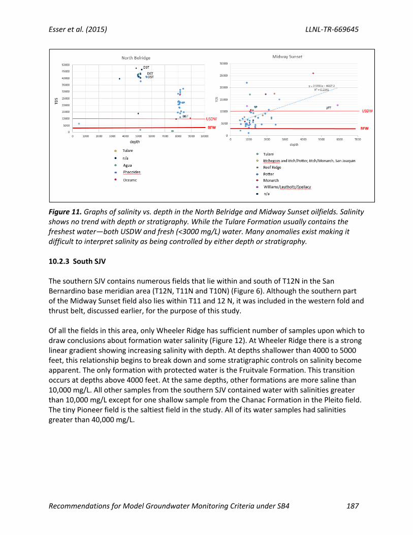
Esser et al. (2015) LLNL‐TR‐669645
Recommendations for Model Groundwater Monitoring Criteria under SB4 187
Figure 11. Graphs of salinity vs. depth in the North Belridge and Midway Sunset oilfields. Salinity shows no trend with depth or stratigraphy. While the Tulare Formation usually contains the freshest water—both USDW and fresh (<3000 mg/L) water. Many anomalies exist making it difficult to interpret salinity as being controlled by either depth or stratigraphy. 10.2.3 South SJV The southern SJV contains numerous fields that lie within and south of T12N in the San Bernardino base meridian area (T12N, T11N and T10N) (Figure 6). Although the southern part of the Midway Sunset field also lies within T11 and 12 N, it was included in the western fold and thrust belt, discussed earlier, for the purpose of this study. Of all the fields in this area, only Wheeler Ridge has sufficient number of samples upon which to draw conclusions about formation water salinity (Figure 12). At Wheeler Ridge there is a strong linear gradient showing increasing salinity with depth. At depths shallower than 4000 to 5000 feet, this relationship begins to break down and some stratigraphic controls on salinity become apparent. The only formation with protected water is the Fruitvale Formation. This transition occurs at depths above 4000 feet. At the same depths, other formations are more saline than 10,000 mg/L. All other samples from the southern SJV contained water with salinities greater than 10,000 mg/L except for one shallow sample from the Chanac Formation in the Pleito field. The tiny Pioneer field is the saltiest field in the study. All of its water samples had salinities greater than 40,000 mg/L.
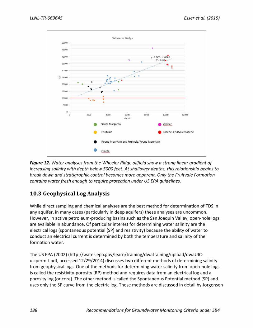
LLNL‐TR‐669645 Esser et al. (2015)
188 Recommendations for Groundwater Monitoring Criteria under SB4
Figure 12. Water analyses from the Wheeler Ridge oilfield show a strong linear gradient of increasing salinity with depth below 5000 feet. At shallower depths, this relationship begins to break down and stratigraphic control becomes more apparent. Only the Fruitvale Formation contains water fresh enough to require protection under US EPA guidelines.
10.3 GeophysicalLogAnalysis While direct sampling and chemical analyses are the best method for determination of TDS in any aquifer, in many cases (particularly in deep aquifers) these analyses are uncommon. However, in active petroleum‐producing basins such as the San Joaquin Valley, open‐hole logs are available in abundance. Of particular interest for determining water salinity are the electrical logs (spontaneous potential (SP) and resistivity) because the ability of water to conduct an electrical current is determined by both the temperature and salinity of the formation water. The US EPA (2002) (http://water.epa.gov/learn/training/dwatraining/upload/dwaUIC‐uicpermit.pdf, accessed 12/29/2014) discusses two different methods of determining salinity from geophysical logs. One of the methods for determining water salinity from open‐hole logs is called the resistivity‐porosity (RP) method and requires data from an electrical log and a porosity log (or core). The other method is called the Spontaneous Potential method (SP) and uses only the SP curve from the electric log. These methods are discussed in detail by Jorgensen
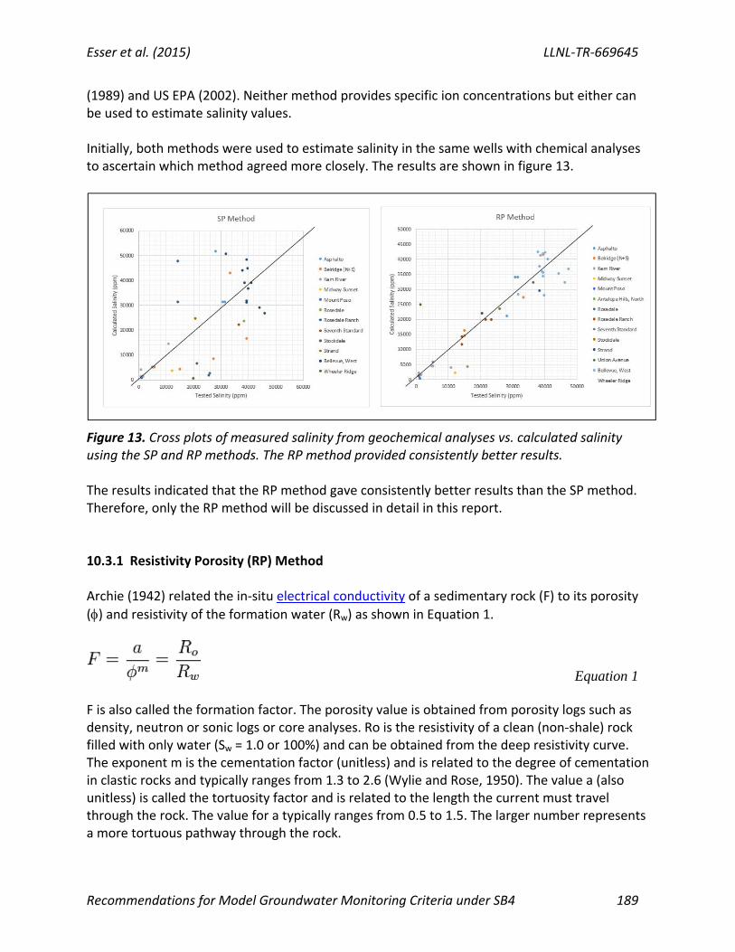
Esser et al. (2015) LLNL‐TR‐669645
Recommendations for Model Groundwater Monitoring Criteria under SB4 189
(1989) and US EPA (2002). Neither method provides specific ion concentrations but either can be used to estimate salinity values. Initially, both methods were used to estimate salinity in the same wells with chemical analyses to ascertain which method agreed more closely. The results are shown in figure 13.
Figure 13. Cross plots of measured salinity from geochemical analyses vs. calculated salinity using the SP and RP methods. The RP method provided consistently better results. The results indicated that the RP method gave consistently better results than the SP method. Therefore, only the RP method will be discussed in detail in this report. 10.3.1 Resistivity Porosity (RP) Method Archie (1942) related the in‐situ electrical conductivity of a sedimentary rock (F) to its porosity
() and resistivity of the formation water (Rw) as shown in Equation 1.
Equation 1 F is also called the formation factor. The porosity value is obtained from porosity logs such as density, neutron or sonic logs or core analyses. Ro is the resistivity of a clean (non‐shale) rock filled with only water (Sw = 1.0 or 100%) and can be obtained from the deep resistivity curve. The exponent m is the cementation factor (unitless) and is related to the degree of cementation in clastic rocks and typically ranges from 1.3 to 2.6 (Wylie and Rose, 1950). The value a (also unitless) is called the tortuosity factor and is related to the length the current must travel through the rock. The value for a typically ranges from 0.5 to 1.5. The larger number represents a more tortuous pathway through the rock.

LLNL‐TR‐669645 Esser et al. (2015)
190 Recommendations for Groundwater Monitoring Criteria under SB4
Equation 1 can be solved for Rw by rearranging the equation (Equation 2):
Rw = Ro * m Equation 2 Equation 2 is an empirical formula which works well for low resistivity waters (< 1.0 ohm‐m) but tends to break down in fresher formation waters where surface conductance of sand grains becomes significant (Alger, 1966). The Humble Equation (Winsauer et al., 1952) is a variant of the Archie Equation that is commonly used in areas with poorly consolidated sands that have porosities ranging from 13‐35%. The Humble Equation uses a = 0.62 and m = 2.15. Because fresher waters are typically found at shallow depths where formations are poorly consolidated and porosities are relatively high, this study uses the Humble Equation variant of the Archie Equation to determine water resistivity (Equation 3).
Rw = Ro * (0.62/2.15) Equation 3
Upon obtaining a value for Rw and calculating the temperature of the zone of interest from the bottom hole temperature on the log header, the TDS of the formation water can be estimated from empirical charts such as those provided by Schlumberger Well Services (1997) (Figure 14). For waters with resistivities greater than 1.0 ohm‐m, salts other than NaCl may contribute significantly to the salinity values (Boeken, 1995). Figure 15 compares the major ion composition of samples from BFW (Base of Fresh Water < 3000 mg/L) and USDW (Underground Source of Drinking Water 3000‐10,000 mg/L) analyses in the SJV. While Na is the major cation in the BFW samples, HCO3 (bicarbonate) is the dominant anion in many, but not all, of the BFW samples. USDW waters on the other hand consistently show Na and Cl as the dominant cation and anion. So, while the RP method may not work well for fresh waters, it should provide a good estimate for waters at TDS concentrations of 10,000 mg/L TDS.

Esser et al. (2015) LLNL‐TR‐669645
Recommendations for Model Groundwater Monitoring Criteria under SB4 191
Figure 14. Rw vs. temperature nomograph used for calculating salinity from water resistivity and temperature (assuming NaCl solutions) from Schlumberger, 1997.
Figure 15. Major cation and anion composition of samples less than 3000 mg/L (BFW) and those ranging from 3000 to 10,000 mg/L (USDW). USDW samples have Na and Cl as the major ions. BFW waters have Na as the major cation but the major anion can be either Cl or HCO3.

LLNL‐TR‐669645 Esser et al. (2015)
192 Recommendations for Groundwater Monitoring Criteria under SB4
10.4 Resistivity‐PorosityMethodResultstoDate Estimates of formation water salinity using the RP method are still underway. The area with the most complete analysis is the western part of the Bakersfield Arch. Electric logs from these fields (and porosity logs where available) were used to iteratively calculate the depth to USDW (10,000 mg/L TDS). An example of the iterative process in the Canfield Ranch field is shown in figure 16. The resulting depths were posted on a map and contoured to determine the depth to USDW across the area (Figure 17). The Rw values were calculated assuming a porosity of 30% in the absence of measured porosity values. Rw values were calculated using the Humble equation (Winsauer et al., 1952).
Figure 16. An example of the iterative process used to determine the depth to USDW (10,000 mg/L) in two wells in the Canfield Ranch oilfield.

Esser et al. (2015) LLNL‐TR‐669645
Recommendations for Model Groundwater Monitoring Criteria under SB4 193
Figure 17. Preliminary contour map showing depth to USDW (10,000 mg/L TDS) estimated from electric log data across the western Bakersfield Arch. Stars indicate the location of well logs used to estimate salinity values. The posted values indicate the approximate depth to USDW. 10.4.1 Sensitivity Analysis Using the RP method to estimate salinities requires that one have accurate values for:
1) Resistivity in a 100% wet sand 2) Porosity 3) The cementation exponent, m 4) The tortuosity exponent, a
These factors are discussed below.
LLNL‐TR‐669645 Esser et al. (2015)
194 Recommendations for Groundwater Monitoring Criteria under SB4
10.4.1.1 Resistivity in a 100% wet sand Of all the variables in the RP equation, the best constrained in this study is the value for Ro. Nearly all of the well files in the CA DOGGR online database contain electric log data from which one can find values for resistivity. However, uncertainties still exist. For example, in eastside fields with fresh formation waters, it is impossible to tell if oil is present within the sands because oil and fresh water both result in high resistivities. Where present in the database, core and mud log information helped to resolve this but, in many cases, the uncertainty still exists. In addition, many wells drilled prior to 1945 were logged with old lateral logs. These logs read far out into the formation but are very sensitive to bed thickness because they average values over a large vertical range. These logs were not used in the study unless no other data were available. Finally, most of the electric logs are stored at scales of 2 inches to 100 feet and resistivity is shown on a linear scale. For the purpose of log analysis, these logs are inferior to the more detailed 5 inches to 100 foot, 0.2 to 2000 ohm‐m logarithmic scale logs because it is more difficult to read accurate resistivity values from the 2 inch linear logs.
10.4.1.2 Porosity Because most well files available in the DOGGR public database do not have porosity logs, porosity usually had to be assumed. Generally, the best quality data in unconsolidated sands are from the density log. The neutron logs are affected more strongly by shale content and the compressional wave on the sonic log is affected by the unconsolidated nature of the sediments in shallow zones. If porosity logs were not available, the average porosity for the zone in that field (or an adjacent field) provided by CA DOGGR (1998) (ftp://ftp.consrv.ca.gov/pub/oil/publications/Datasheets/Dtasheet_vol_1.pdf, accessed 3/29/2015) was used. As a last resort, a value of 30% was assumed as this is a typical value for unconsolidated sands in the SJV. A sensitivity analysis was conducted for porosity in which the porosity was varied from 26 to 33% while all other variables were held constant to determine the sensitivity of the RP method to porosity values. The results are shown in Table 1. Over the given range of porosities, water resistivity (Rw) estimates varied from 0.22 to 0.37 ohms and salinity varied from 11,000 to 19,500 mg/L. This is certainly a large source of error and makes it clear that the values for the RP method, in the absence of porosity log data, must be used as a guideline only. For accurate results, regulatory agencies should require operators to collect accurate porosity measurements from the aquifer when attempting to use this method.

Esser et al. (2015) LLNL‐TR‐669645
Recommendations for Model Groundwater Monitoring Criteria under SB4 195
Table 1. Sensitivity analysis to porosity. The red box shows the most likely values. An uncertainty in porosity of 7% can cause an 8000 mg/L uncertainty in calculated TDS values using the RP method.
10.4.1.3 Cementation Factor A similar sensitivity analysis was performed for the cementation exponent, m. Guyod (1944) notes that poorly cemented sands range from 1.4 to 1.7 however, Values for m are dependent upon values for a, the tortuosity factor. In this study the Humble Equation was used because it was developed to analyze poorly consolidated sands in the Gulf Coast. The Humble Equation (Winsauer et al., 1952) uses an m value of 2.15 when the value for a is 0.62. Therefore, the sensitivity analysis for the cementation factor was used for values at, or less than, 2.15. While holding other variables constant (including a = 0.62), m was varied from 1.7 to 2.15. The resulting salinities varied from 8500 to 14,000 mg/L (Table 2).

LLNL‐TR‐669645 Esser et al. (2015)
196 Recommendations for Groundwater Monitoring Criteria under SB4
Table 2. Sensitivity analysis to the cementation exponent, m. The red box shows the most likely value using the Humble equation. However, some authors note theat the value for m in poorly consolidated sediments can be less than 2.0 if a = 1.0 (Guyod, 1944).
10.4.1.4 Tortuosity factor, a A sensitivity analysis was performed for the tortuosity factor, a. The Archie equation (Archie, 1942) uses a value of 1.0 for a, while the (1949) equation uses a value of 0.81 and the Humble equation (Winsauer et al., 1952) a value of 0.62. While holding other variables constant, a was varied from 0.5 to 1.0. The resulting salinities varied from 11,000 to 22,000 mg/L (Figure X).
Table 3. Sensitivity analysis to the tortuosity factor, a. The red box shows the most likely value using the Humble equation.

Esser et al. (2015) LLNL‐TR‐669645
Recommendations for Model Groundwater Monitoring Criteria under SB4 197
11 APPENDIX:OVERVIEWOFDEPTH‐DISCRETEMULTILEVELGROUNDWATER
MONITORINGTECHNOLOGIES:FOCUSONGROUNDWATERMONITORINGINAREASOFOILANDGAS
WELLSTIMULATIONINCALIFORNIA
Prepared by:
John Cherry1, Beth Parker1, Murray Einarson2, and Steven Chapman1, Jessica Meyer1
1 G360 Centre for Applied Groundwater Research University of Guelph 50 Stone Road East
Guelph, ON Canada N1G 2W1 [email protected] [email protected] [email protected] [email protected]
2 Haley Aldrich
1956 Webster Street, Suite 450 Oakland, CA 94612
Prepared for:
Lawrence Livermore National Laboratory
For the SB4 Groundwater Monitoring Expert Advice Project
June 29, 2015

Overview of Depth-Discrete Multilevel Groundwater Monitoring Technologies:
Focus on Groundwater Monitoring in Areas of Oil and Gas Well Stimulation in California
Prepared by:
John Cherry1, Beth Parker1, Murray Einarson2, Steven Chapman1, Jessica Meyer1
1 G360 Centre for Applied Groundwater Research University of Guelph 50 Stone Road East
Guelph, ON Canada N1G 2W1 [email protected] [email protected]
[email protected] [email protected]
2 Haley Aldrich
1956 Webster Street, Suite 450 Oakland, CA 94612
Prepared for:
Lawrence Livermore National Laboratory U.S. Department of Energy
For the SB4-WST Project
June 29, 2015

Author’s disclosure: The authors of this review have no financial ties to the companies that manufacture and sell MLSs, except for Murray Einarson, who invented and patented the CMT system and receives royalties from Solinst Canada Ltd. Although John Cherry co-invented the Solinst Waterloo system, held a joint patent and received royalties in the past, the patents on this system have long since expired and he no longer receives royalties since 2000.
MLS - ii FINAL VERSION (6/29/2015)
Table of Contents List of Figures ................................................................................................................................................ v List of Tables ............................................................................................................................................... vii 1.0 Synopsis................................................................................................................................................... 1 2.0 Introduction ............................................................................................................................................ 3
2.1 Site Conceptual Models and MLSs ...................................................................................................... 3
2.2 Purpose and Scope of this Document ................................................................................................. 5
2.3 Importance of Multilevel Monitoring in the SB4 Program ................................................................. 6
2.4 Depth-Discrete Multilevel data Collection During Site Characterization and Long-term Monitoring 7
2.5 issues Related to Monitoring Shallow and Deep Groundwater ......................................................... 8
2.6 A Long History of MLS Installations in California ................................................................................ 9
3.0 Options for SB4 Groundwater Monitoring ........................................................................................... 11 4.0 Engineered MLS systems ...................................................................................................................... 13
4.1 Overview of Four Commercially-Available MLS systems .................................................................. 13
4.1.1 Solinst CMT System ............................................................................................................. 13 4.1.2 Solinst Waterloo System ..................................................................................................... 13 4.1.3 Water FLUTe System ........................................................................................................... 14 4.1.4 Westbay MP System ........................................................................................................... 16
4.2 Key MLS advantages ......................................................................................................................... 16
4.3 General Design Objectives for MLS Selection ................................................................................... 17
4.4 Importance of MLS Purging .............................................................................................................. 20
4.5 Installation methods ......................................................................................................................... 22
4.5.1 Temporary Casing and Backfill Method .............................................................................. 23 4.5.2 Installations of Engineered MLSs in Open Stable Rock Holes ............................................. 25 4.5.3 Installations of Engineered MLSs in Multi-Screened Cased Wells ...................................... 25 4.5.4 Methods for Constructing Multi-Screened, Steel-Cased Wells .......................................... 27
4.6 Well Development and Drilling Considerations ................................................................................ 29
4.7 QA/QC and Integrity of Seals Between Monitoring Intervals ........................................................... 31
4.7.1 Backfilled Waterloo and CMT Systems ............................................................................... 31 4.7.2 Westbay Systems ................................................................................................................ 31 4.7.3 Water FLUTe System ........................................................................................................... 32 4.7.4 Westbay or Water FLUTe MLS Installed in Multi-Screened Wells ...................................... 33
4.8 Example California MLS Installation scenarios ................................................................................. 33
4.8.1 Shallow MLS Installations to 200 feet ................................................................................. 34 4.8.2 Intermediate MLS Installations down to 500-600 feet ....................................................... 34 4.8.3 Deep Installations between about 500 feet to 1,500 feet ................................................. 34 4.8.4 Very Deep MLS Installations from 1,500 to 4,000 feet ....................................................... 35
4.9 Sampling methods ............................................................................................................................ 35
MLS - iii FINAL VERSION (6/29/2015)

4.9.1 Water FLUTe System ........................................................................................................... 35 4.9.2 Westbay System .................................................................................................................. 35 4.9.3 Solinst Waterloo System ..................................................................................................... 36 4.9.4 CMT System ........................................................................................................................ 36
4.10 Pressure Monitoring Methods ........................................................................................................ 37
4.11 Decommissioning Methods ............................................................................................................ 37
5.0 Discussion .............................................................................................................................................. 40 5.1 Performance in Presence of Oil ........................................................................................................ 40
5.1.1 Water FLUTe System ........................................................................................................... 40 5.1.2. Westbay MP System ........................................................................................................... 40
5.2 MLS Design Considerations ............................................................................................................... 41
5.3 MLS Improvements and Adaptations ............................................................................................... 41
6.0 Summary and Conclusions .................................................................................................................... 43 7.0 Acknowledgements ............................................................................................................................... 45 8.0 References ............................................................................................................................................ 46 9.0 Figures ................................................................................................................................................... 50 APPENDICES ................................................................................................................................................ 73
Appendix A: History of Development of Commercial MLSs ................................................................... 73
MLS - iv FINAL VERSION (6/29/2015)
List of Figures Figure 1. Example high resolution head profile showing large vertical gradients over short vertical intervals , providing detailed understanding of the flow system. (Source: Meyer et al., 2014).
Figure 2. Schematic of insights from high resolution head profiles showing distinct inflections and large head changes aiding detailed understanding of the flow system, versus lower resolution blended heads from longer monitoring intervals providing an inaccurate view of the flow system. (Source: Meyer et al., 2014).
Figure 3. Westbay completions in California (Source: provided by Westbay Instruments, a Division of Nova Metrix Ground Monitoring (Canada) Ltd.).
Figure 4. Three general approaches to obtain vertical profiles: (a) well nest with multiple casings with short screens installed in a single hole with sand packs surrounding the screens and bentonite seals between the sandpacks, (b) well cluster with short-screened wells at different depths in individual holes, and (c) multilevel well system. (Source: adapted from Einarson 2006).
Figure 5. Use of centralizers for nested wells to ensure good seals between monitored zones: (a) installation without centralizers and imperfect seal between zones, (b) centralizers keeping casings centered in the hole and superior seals between zones, and (c) centralizer design for three zone nested well. (Source: Einarson 2006).
Figure 6. Scenario with well cluster causing short-circuiting due to positioning of the well screens with presence of vertical gradients. (Source: Einarson 2006).
Figure 7. Schematics of generic MLS installation approaches: (a) backfilled system with sand packs around the monitoring intervals and bentonite seals between sand packs (unconsolidated or rock); (b) system in open rock walled hole with packers between open intervals, (c) system installed inside multi-screen casing with packers (adapted from Einarson, 2006), and (d) system in hole fully sealed with a flexible liner, with monitoring intervals formed of a permeable mesh.
Figure 8. Schematic of Solinst CMT system (Source: Einarson 2006).
Figure 9. CMT system (a) CMT tubing, (b) typical CMT intake port, and (c) CMT tubing coil (Source: Einarson and Cherry, 2002).
Figure 10. Schematic of Solinst Waterloo multilevel system version with packers (Source: Einarson 2002).
Figure 11. Installation options for Waterloo multilevel system (Source: courtesy of Solinst Canada Ltd.).
Figure 12. Schematic of modified Waterloo System with fifteen ports for installation in sonic casing (Source: Parker et al., 2006).
Figure 13. Schematic of Hybrid Waterloo System with up to nine internal ports and two external piezometers for installation in 6-in tricone holes or 5-in PQ-cored holes (Source: Chapman et al., 2015).
Figure 14. Schematic of (a) FLUTe liner installation procedure with liner attachment to casing, water addition and liner descent below water table, and (b) example (1 port) Water FLUTe groundwater sampling.
MLS - v FINAL VERSION (6/29/2015)
Figure 15. Water FLUTe system: (a) installing Water FLUTe system down 6-in borehole, and (b) completed installation (Source: courtesy of FLUTe).
Figure 16. Three Water FLUTe options : (a) the Standard Water FLUTe well-suited for very deep to shallow conditions with positive displacement pumping , (b) the Special Water FLUTe has some compromises to reduce cost, and (c) the Shallow Water FLUTe system is limited to water tables <25 ft below surface with peristaltic pumping at the surface. All the Water FLUTes have head, and transducer measurements.
Figure 17. Schematic of Westbay MP system (Source: courtesy of Westbay).
Figure 18. Components of the Westbay MP System (Source: courtesy of Westbay).
Figure 19. Westbay completion options (Source: provided by Westbay Instruments, A Division of Nova Metrix Ground Monitoring (Canada) Ltd.).
Figure 20. Options for pumping, testing and monitoring with the Westbay MP system (Source: Einarson 2006).
Figure 21. Example of geophysical logs from an air-rotary drilled borehole with 6-in bit in sedimentary rock from a typical groundwater monitoring well completed in fractured bedrock at Site 300, a DOE CERCLA site in the Altamont Hills, CA. The caliper log shows significant borehole enlargement (washout) in the 80 to 95 ft depth range.
Figure 22. Well development considerations based on drilling method and borehole damage.
Figure 23. Example showing well nest design with four separate casings and screens in a single 200 ft deep borehole in Stockton, CA (Source: O’Leary et al., 2012).
MLS - vi FINAL VERSION (6/29/2015)

List of Tables Table 1. Options for multilevel groundwater monitoring.
Table 2. Multilevel Monitoring Systems (MLS) commercially available (Source: ITRC [Interstate Technology & Regulatory Council], 2015).
Table 3. Water FLUTe differences.
MLS - vii FINAL VERSION (6/29/2015)
1.0 Synopsis Depth-discrete, multilevel monitoring refers to engineered Multilevel Systems (MLSs) installed in single boreholes for efficient monitoring of hydraulic head (i.e. fluid pressure) and groundwater sampling at many different depth intervals in each hole. It is important that the monitored intervals or zones be reliably isolated from the zones above and below. It is also important that annular spaces of the unmonitored sections between the monitor intervals be filled with reliable seals (the annular seals). There are several well-established versions of MLSs available from commercial vendors and these are the focus of this document. This document does not examine other MLSs produced in academia or by government agencies for use on their own projects but not widely available. Commercial MLSs entered the marketplace in the late 1970's with one technology offered by one company. Now there are four primary systems (the Westbay MP® system, the Solinst Waterloo system, the Solinst CMT system, and the Water FLUTe™ system), with variations of each offered by three companies: Westbay® Instruments (a division of Nova Metrix Ground Monitoring (Canada) Ltd.), Solinst Canada Ltd., and Flexible Underground Liner Technologies (FLUTe™). Each MLS has specific design features that provide advantages and sometimes disadvantages in various borehole or hydrologic circumstances, and corresponding niches particular to its relative advantages, which are strongly related to the nature of the intended use and site-specific hydrogeologic conditions. The commercially available MLSs have a long record of groundwater monitoring in California and globally at depths ranging from tens to thousands of feet. This review document describes the various MLSs and their attributes with emphasis on relevance to area-specific and regional groundwater monitoring requirements in support of California Senate Bill (SB4) which requires groundwater monitoring in areas of oil and gas well stimulation. The hydrogeologic complexity in California’s oil and gas producing regions favors application of MLS technologies rather than conventional monitoring wells, so that each hole drilled for groundwater monitoring maximizes the insight gained from multiple hydrogeologic units, both those serving as aquifers and aquitards. Given the depths and multiple hydrogeologic units present in petroleum rich sedimentary basins, multilevel completions offer the best prospects for cost-effective, scientifically defensible data to assess potential impacts or lack thereof from unconventional oil and gas extraction.
The subject of QA/QC protocol and testing of annular seals is often a focus of attention in the context of MLS systems. As discussed later in this document, assessments of the integrity of the seals after completion of the installations can be inconclusive. Minimizing this uncertainty is, in fact, one of two reasons why engineered MLS systems were developed in the first place. The other reason for development of MLSs was to achieve the most cost effective use of each borehole for groundwater system understanding and in particular to obtain more detailed information about the groundwater conditions at the borehole location than can be obtained by any other means. The developers of the four commercially available MLS technologies were consultants or researchers who worked on projects where early attempts at multi-level monitoring — typically done with nested wells (i.e., multiple pipes in a single borehole) — were fraught with failed seals and an inadequate number of monitored zone. It was often difficult to judge whether or not the seals between zones were working. Consequently, they developed engineered MLS systems that, by design, dramatically improved the performance and reliability of the annular seals between the monitored zones while providing more monitored zones. The key design improvement — which is common to all of the commercial MLS systems on the market — is that there is only one pipe, tube or sleeve placed in the borehole, not multiple pipes, tubes, or sleeves that are difficult to seal in between. Thus, one must consider the superior design of engineered MLS systems as a key (and perhaps the most important) prescriptive QA/QC element for reliable collection of high-quality, multi- depth groundwater data.
MLS - 1 FINAL VERSION (6/29/2015)

Engineered MLS systems have been used extensively in California, with some of the first installations conducted more than 25 years ago. A conservative estimate is that more than 2,000 MLS have been installed to date in California to depths up to 2,000 feet. Consequently, the primary goal of this report is to objectively present the capabilities and attributes of the commercially available and relevant engineered MLS systems – which are available today “off the shelf” – in support of the SB4 Regional and Area-Specific monitoring requirements. MLS technologies are now well advanced and suitable for an immediate major role in WST monitoring in California and elsewhere while further technology advances occur through experience and research.
MLS - 2 FINAL VERSION (6/29/2015)

2.0 Introduction One of the most important discoveries made during the last five decades of groundwater research is that the distributions of dissolved contaminants in the subsurface are generally spatially complex, especially in the vertical direction. This is due to a number of factors, most importantly the geologic complexity that imparts complexity onto the hydraulic conductivity (K) distribution and the spatial distribution of most types of contaminant sources. This discovery was made first in studies of shallow contaminants in unconsolidated deposits in the 1970’s and 1980’s associated with landfills, sewage lagoons, septic systems, and chlorinated solvent sites (Cherry et al. 1981, MacFarlane et al. 1983, Reinhard et al. 1984, Smith et al. 1987, Robertson et al. 1991, van der Kamp et al. 1994) by installing multiple sampling devices in a single borehole facilitating the collection of groundwater samples from up to 20 different depths. These early multilevel systems, improvised and produced by contaminated site investigators with features adapted for site-specific conditions, set the stage for the advent of MLSs manufactured and marketed commercially for many types of groundwater monitoring needs. 2.1 SITE CONCEPTUAL MODELS AND MLSS The main purpose in the use of MLSs is to serve the needs for rigorous development of Site Conceptual Models (SCMs) of hydrogeologic environments. This is done through acquisition of data profiles from boreholes and MLSs are a key technology in this endeavor. Following the description in the SB4 report (Esser et al. 2015), SCMs by their very nature, are imperfect and incomplete, and will always be a work-in-progress. These models are a compilation and integration of relevant data needed to characterize and protect groundwater resources at the area and regional scales under SB4. SCMs consist of three spatial dimensions and a fourth temporal dimension. Probable pathways for fluid migration, estimates of groundwater flow direction and velocity, and solute transit times are critically important components of SCMs for SB4 monitoring. Ultimately the SCM provides the basis for interpreting spatial and temporal data and identifying the location and timeframe for groundwater quality impacts related to well stimulation activities. Although SCMs will always be somewhat imperfect and incomplete, they become refined and more robust with time as data from interdisciplinary sources are incorporated into the model. Initially, hypotheses and assumptions are challenged and often refuted by subsurface data collected early in the development of the SCM. Subsequent analysis and hypotheses testing is performed and data gaps are filled in an iterative process that ultimately enhances the quality of the SCM at different spatial scales. In this way, the SCM is strengthened or “validated” and becomes the primary tool for designing monitoring programs, identifying potential risk to receptors, and developing targeted, cost-effective corrective action plans. In order to be an effective decision-making tool for protecting groundwater resources under SB4, the SCM must integrate a broad range of multi-disciplinary data from both the oil and gas and hydrogeology disciplines at a range of spatial and temporal scales. The main types of information are geology, hydrogeology and geochemistry. The expertise for each of these earth science disciplines is different and generally requires a team of specialized individuals involved in interdisciplinary analyses in the overall process of conceptual model development. The foundation of the SCM is a geologic model that defines the distribution of geologic materials, generally sedimentary strata, including their bulk hydraulic conductivity, lateral continuity, and geochemical reactivity. Structural features, such as faults and fracture corridors, are also critical aspects of the geologic model, especially in the context of transmissive geologic pathways for stimulation and hydrocarbon reservoir fluids and how they may be altered due to anthropogenic activities. In addition to the well stimulation target zone, any geologic
MLS - 3 FINAL VERSION (6/29/2015)

strata that contain methane are potential contaminant sources and these gas rich zones can occur anywhere in the stratigraphic column. The SCM should endeavor to identify these gas source zones and their location relative to well stimulation activities. Although there is still considerable debate about how and under what specific conditions well stimulation operations might negatively impact groundwater quality, it is generally recognized that wellbore-integrity failure, especially under pressurized conditions, represents a real risk to protected groundwater (Jackson et al. 2014; CCA report 2014). Some of the risk is due to mobilization of fluids in the overlying strata that are penetrated to reach the stimulation target zone. Other identified risks to groundwater from well stimulations in California include operational spills and waste disposal practices (CCST et al., 2014). Perhaps the most significant challenge for developing technically defensible SCMs is identifying connections between geologic and anthropogenic pathways capable of transmitting fluids, including methane and brines, and negatively impacting protected groundwater. The SCM uses the geologic model as the framework and incorporates hydraulic properties such as hydraulic conductivity and hydraulic head under both unstressed and stressed conditions. An integral part of the SCM is the characterization of the hydrostratigraphy and the recognition of discrete hydrostratigraphic units, also known as hydrogeologic units, mainly aquifers and aquitards, depending primarily on bulk hydraulic conductivity related to interconnected porosity and fractures at all spatial scales. For those units that are aquifers, the most important component of the hydraulic conductivity is the component that is generally conformable or parallel to the aquifer’s stratigraphic orientation and for aquitards, it is primarily transverse or perpendicular to this orientation. Groundwater flow indicators or natural tracers, such as stable isotopes of water, tritium, carbon-14, helium, and others provide insight into local- and regional-scale groundwater flow patterns, including flow along natural and man-made preferential pathways that may be conformable or transverse to the hydrostratigraphy. In the context of SCMs for well stimulation impacts, an understanding of geochemical and biogeochemical processes is crucial to interpreting multi-disciplinary groundwater monitoring data and identifying impacts from well stimulations. The biogeochemical component of the SCM concerns reactive transport processes related to the interaction of both natural and anthropogenic dissolved constituents with the rock matrix and the potential transformation or utilization of these constituents by the indigenous microbial community. The biogeochemical component is especially important concerning stray methane that, due to buoyancy, can migrate upward along preferential pathways or be attenuated by biogeochemical processes that may or may not cause secondary negative water quality impacts. The spatial distribution of hydrostratigraphic units, also known as hydrogeologic units, can serve as the framework for local- and basin-scale numerical groundwater models. For example the USGS Central Valley Hydrologic Model was developed as a decision-making tool to simulate groundwater flow, manage groundwater resources related to land usage, primarily agricultural impacts in the context of surface and groundwater interactions and long-term climatic trends (Faunt, 2009). Many studies have shown the importance of measuring hydraulic heads at many vertical depths at a single monitoring location (Cherry et al. 2005, Meyer et al. 2008, Meyer et al. 2014). Hydraulic head drives the movement of groundwater and contaminants in the subsurface, which is why characterization and monitoring of hydraulic head is an important part of developing a robust SCM in support of SB4 groundwater monitoring programs. Meyer et al. (2014, 2008) showed the value of high resolution (i.e., detailed, depth discrete, minimally blended) head profiles derived from multilevel systems with many ports for flow system characterization by indicating the boundaries of hydrogeologic units and providing highly accurate hydraulic head and vertical gradient data (Figure 1). Hydraulic information derived from
MLS - 4 FINAL VERSION (6/29/2015)
long screened wells, open boreholes or well clusters with too few wells is likely to lead to inaccurate delineation of hydrogeologic units, over-estimates of aquitard thickness, and inaccurate hydraulic head and vertical gradient values (Figure 2). This poor characterization of the flow system can lead to misleading conceptual models and poor predictive capability for flow and contaminant transport behavior (Meyer et al. 2014). Finally, detailed vertical profiles of hydraulic head can be used along with geologic data to identify specific vertical horizons that form strong barriers or impediments to vertical groundwater flow. Such knowledge is vital to assess possible migration of WST fluids injected at great depths to overlying shallow groundwater sources. Depth-discrete groundwater monitoring and measurement of vertical head distributions through time is important for most hydrogeologic investigations, but is particularly important for SB4 characterization and monitoring programs given their objectives. The ability to detect and quantify changes in groundwater chemistry in different vertical zones over time (e.g. possibly resulting from WST activities) is clearly a fundamental objective of SB4 monitoring in California. Measuring vertical head profiles over time is also very important. For example, changes in vertical head profiles in a MLS could indicate breaches in aquitards, (e.g. by nearby WSTs). Finally, SB4 monitoring requires definition of the potential directions of fluid migration from WSTs, which is determined largely by the direction and magnitude of the subsurface hydraulic gradients. Installation and monitoring of MLSs in an oil field where WSTs are being performed or are planned is the path to obtain this important information. 2.2 PURPOSE AND SCOPE OF THIS DOCUMENT This document is a review of commercially available MLSs. Prior to this, the most recent review of MLSs was that by Einarson (2006); however there have been major advances in the technologies in the past decade and much accumulated experience to guide how MLSs can be most effectively used. The emphasis of this review is on relevance for local and regional monitoring to discern and understand the impacts of oil and gas developments in California related to well stimulation treatments (WSTs) in support of California Senate Bill 4 (SB4) monitoring requirements. The groundwater monitoring needs relevant to SB4 are broad, from monitoring in shallow unconsolidated deposits generally less than 100 feet deep, to zones as much as 3,000-4,000 feet deep in indurated geologic units (i.e. sedimentary rock such as sandstone and shale). The geology most relevant to WSTs in California includes many stacked, flat lying or dipping geologic layers or hydrogeologic units that are commonly fractured and faulted. Additional hydrogeologic complexity is created by anthropogenic disturbances of the subsurface due to incompletely sealed oil and gas wells, old exploration holes, and / or water wells that cross-connect hydrogeologic units. Typically there are several hydrogeologic units acting as aquifers and many as confining beds (aquitards). Therefore the main challenge in designing groundwater monitoring networks involves delineating and characterizing all hydrogeologic units, and then choosing the most important hydrogeologic units to target for ongoing long-term monitoring. This review is limited to commercially available MLSs that are broad in purpose, intended to provide data on fluid pressure (i.e. hydraulic head) and also allow repeated groundwater sampling for laboratory analyses of chemical composition. They also allow sealing of all parts of the borehole that are not monitored. There are other technologies for obtaining multilevel data for only one of two main objectives alone, fluid pressure or fluid sampling, but not both in the same hole. Those technologies are not included in this review. This review considers only commercially available MLSs. Several other MLSs are described in the literature (e.g. Bishop et al. 1991; Boyle 1992; Schirmer et al. 1995; Ducoommun et al. 2013) but, although these systems had particular usefulness for which they were developed, they did not enter the commercial marketplace and have not been widely applied. Each of the commercial MLSs described in this document entered the marketplace between 15 and 38 years ago, and each has been
MLS - 5 FINAL VERSION (6/29/2015)
much improved based on accumulated experience. There are four commercial MLSs and each has key design features distinguishing it from the others: the Westbay MP® system, the Solinst Waterloo system, the Solinst CMT™ (Continuous Multichannel Tubing) system and the Water FLUTe™ system. All have been invented in and are manufactured only in the United States or Canada. While manufacturing is done in North America (New Mexico, British Columbia and Ontario), there have been thousands of MLS installations outside of North America, especially in Europe and South America. Although the commercial MLSs have been used in many types of hydrogeologic environments in California and globally, the publically available literature on these applications is sparse. Most of the information is contained in project specific site reports that are not available, or not readily obtainable. Each of the four MLS types has versions tailored to site-specific needs and each has limitations and preferred niches. For example, the CMT™ system is limited to depths of about 200 feet below surface and has been used almost entirely in overburden. In contrast, the Westbay MP® system is most commonly used at depths >500 feet (ft) and has been used at depths >5,000 ft, although it is also used at shallower depths. The Water FLUTe™ can be used most effectively in bedrock holes 5 inches in diameter or larger, but also can be installed in small diameter holes. The other MLSs are generally limited to holes with diameters of 6 inches or less, mostly between 4 - 6 inches. All of the commercially available MLSs are relevant to WST issues because of the wide range of potential contaminants and release points, some shallow and some deep and the many types of geologic conditions in the petroliferous basins of California. 2.3 IMPORTANCE OF MULTILEVEL MONITORING IN THE SB4 PROGRAM Problems and issues associated with blending in long screened wells are well-established (Einarson, 2006; many others). Such blending influences measurements of hydraulic head and hydraulic conductivities used to characterize the flow system and inform and calibrate numerical models, and significantly biases groundwater concentration data, decreasing our ability to detect small but time critical breakthrough of solutes. Groundwater geochemistry is remarkably variable with depth in the subsurface, even in relatively homogeneous aquifers that are only tens of feet thick. The vertical variations in groundwater geochemistry are orders of magnitude more variable at the scales of SB4 monitoring, which span hundreds to thousands of feet vertically, from shallow Quaternary fresh-water aquifers to deep saline, oil-bearing strata. Consequently, it is important to be able to collect groundwater samples at a single location from multiple depths corresponding to different hydrogeologic units. Hence, the MLS provides profiles of hydraulic head and hydrochemistry versus depth for characterization of the hydrogeologic system. Profiles with enough detail obtained from a sufficient number of locations can provide the framework for 3-dimensional understanding. Regional groundwater monitoring performed in California (e.g., Groundwater Ambient Monitoring and Assessment or GAMA program) has historically focused on collecting groundwater samples from existing long-screened water supply and monitoring wells (Burton and Belitz 2008, Landon et al. 2010, Singleton et al. 2011). Those samples are, by nature, blended samples from many different depths owing to the long screened intervals of those wells. Blended groundwater samples typically yield conflicting and often mutually-exclusive geochemical results, such as high concentrations of dissolved iron (indicating anaerobic conditions) and high concentrations of dissolved oxygen (indicating strongly aerobic conditions). The reason for this is simply that the well is screened across different hydrogeologic units, at least one of which contains anaerobic groundwater and others which are aerobic. Water from each unit flows into the well when it is pumped, becoming blended in the well and pump column, and subsequently being collected in a sample vial. Similar in-well blending of groundwater complicates groundwater age determination and efforts to determine groundwater recharge conditions (an
MLS - 6 FINAL VERSION (6/29/2015)

important parameter in paleoclimate studies) using cutting-edge (and expensive) analytical techniques. Ambient flow in open holes and long-screened wells can also yield misleading and ambiguous data concerning hydraulic head and solute concentrations (e.g. Elci et al. 2001). The length of the monitoring interval that is most appropriate depends on the site-specific hydrogeology and the types and ways in which the chemicals enter the groundwater domain of interest. The collection of water samples and the analysis of the samples for many constituents and isotopes is an expensive endeavor per sample. Therefore, if the location of the water sample within the groundwater system is not known accurately, the effort can be minimally insightful. Recognizing this significant uncertainty, geochemists in California and elsewhere have recently made significant efforts to increase the resolution of their groundwater sample collection methods, by collecting samples from multi-level monitoring wells with much shorter well screens or by collecting groundwater samples and measuring inflow rates at multiple depths in actively pumped wells to calculate aquifer concentrations of the target solutes (Izbicki et al. 2005; O’Leary et al. 2012). As discussed in more detail below, engineered MLSs provide high-resolution samples of groundwater from discrete intervals that yield more accurate measurement of depth-dependent groundwater geochemistry, translating to much more accurate determinations of groundwater age and paleoclimatic conditions. Moreover, eliminating sample blending effectively lowers the detection limit of analytes that may indicate possible impacts from WST activities compared to blended samples from traditional long-screened wells. Blended samples greatly reduce the likelihood of detecting significant changes in groundwater chemistry early in the process of change. The leading edges of contaminant plumes are prone to go undetected in blended samples. Blended samples may represent the water quality relevant to water well users of the moment, but are not effective for observing the early changes in the larger groundwater resources in the aquifers. Without detection of early changes, there is no sentry monitoring. 2.4 DEPTH-DISCRETE MULTILEVEL DATA COLLECTION DURING SITE CHARACTERIZATION AND LONG-TERM MONITORING The creation of MLSs was driven primarily by the desire to obtain much more information from each monitoring site than is feasible economically and technically by installation of well clusters or well nests. The precursors for the commercial MLSs were multilevel systems aimed at obtaining detailed profiles of water chemistry, such as the bundle wells used for example by Cherry et al. (1983) in sand aquifers for landfill plume delineation, or the precursor to the Westbay system that Patton (1973) used to measure hydraulic head profiles in bedrock for mountain slope stability analysis. Both of these endeavors were founded on the premise that the necessary spatial scale of data acquisition in the site characterization phase cannot become known until sufficient data have been obtained to achieve the essential understanding. Therefore at the earliest stage of an investigation, the vertical spacing between data acquisition intervals in multilevel sampling or pressure monitoring systems is set as small as is technically practical to determine the level of detail most appropriate for the desired degree of understanding. For contaminant plumes in shallow cohesionless sandy aquifers, bundle wells provided enough detail in the hydrochemical profiles for delineation and understanding of the Borden landfill plume (Cherry et al. 1983) and chlorinated solvent plumes (Guilbeault et al. 2005). This level of detail in the characterization phase eventually became known as high resolution profiling, and became applied to hydraulic head profiling using the Westbay MLSs (e.g. Meyer et al. 2006; Meyer et al. 2014) as well as hydrochemical profiling using the Waterloo system (e.g. Parker et al. 2007 ) and the CMT system (Einarson and Cherry 2002).
MLS - 7 FINAL VERSION (6/29/2015)
The RCRA (1976, 1980) and CERCLA (1980) legislation and related regulations and guidance unleashed a momentous surge in groundwater monitoring in the 1980's, which initially had much diversity in the methods used. However, soon groundwater monitoring practice evolved and stabilized into the prescriptive use of conventional monitoring wells and well clusters, with only a few wells in each cluster, for which there are ASTM standards and many guidance documents (e.g. ASTM-D5092-04). Gradually over the next decade or two, it became recognized that conventional monitoring wells are not an effective tool for site characterization and SCM development. New tools and approaches were developed aimed at effective and efficient site investigations for characterization and conceptual model building (i.e. the site characterization phase). This phase is followed by the site monitoring phase, for which the design of the monitoring network can be based in the SCM founded on the site characterization results. The MLSs described in this document are commonly used in both phases of contaminated site investigations, the characterization and monitoring phases, but the nature of the uses is different because in the characterization phase, the goal is to delineate and understand the hydrogeology and hydrochemistry and their processes, while in the monitoring stage the goal is to establish the baseline conditions for comparison to results of cost-effective long-term monitoring of changes in groundwater quality. In contaminated site investigations that usually concern small areas, with site remedial decisions taken over many years or even decades, it has been feasible to separate the characterization phase from the long-term monitoring phase. A key consideration in the selection and design of a MLS is specification of the number of monitoring intervals, and this has much to do with the phase of the study, characterization or long-term monitoring, in which the decisions are being made. For the SB4 applications of MLSs in the petroliferous basins in California, the early phase of investigation is most appropriately viewed as being the system characterization phase, because the data needed to create SCMs need to be acquired and analyzed before decisions are made for establishment of long-term monitoring networks. In this context there is commonly need to use as many monitoring intervals as is technically and economically feasible in each hole, to get as much detail as possible about both the aquifers and aquitards that make up the groundwater system. The aquitards are important because, as confining or semi-confining hydrogeologic units, they generally govern the groundwater flow pathways and hydrochemistry. The maximum number of monitored zones is different for each of the various commercial MLS systems. For example, the CMT system allows for a maximum of seven intervals, which can be enough for shallow monitoring, generally less than 150-200 feet. The Westbay system because it is entirely modular allows for a monitoring zone every 10-15 feet of hole with the limitation on the total number of monitoring intervals in the hole being primarily the length of the hole. This allows for high resolution monitoring in all parts of a deep hole and is the only MLS that offers that capability. The Water FLUTe system is limited in the number of monitoring intervals in small diameter holes, such as less than 4 inches where only a few intervals can be used, but in holes greater than 6 inches the number of monitoring intervals that can be accommodated becomes much more substantial (e.g. more than fifteen) and increases with borehole or multi-screen casing diameter. Given the expense of installing MLSs, it is desirable that they play a valuable role in both the characterization and long-term monitoring phases. In the characterization phase all the monitoring intervals are relevant until adequate system understanding is achieved. Later, routine monitoring may focus on only a subset of the monitoring intervals, i.e. those deemed most essential for observing possible impacts. 2.5 ISSUES RELATED TO MONITORING SHALLOW AND DEEP GROUNDWATER Concerns about groundwater contamination related to WSTs pertain to potential sources of contamination originating both at land surface, including spills and leaks of hydrofracturing chemicals,
MLS - 8 FINAL VERSION (6/29/2015)

fuels and flow-back water, and also from deep sources, such as stray gas and chemical additives used in the stimulation treatments, which is a key driver for the SB4 legislation. MLS is a broad term that encompasses many types of engineering designs. The four commercially available systems are: the Westbay MP® system, referred to hereafter as the Westbay system, the Solinst Waterloo™ system, the Solinst CMT™ system and the Water FLUTe™ system. The Waterloo System refers to the generic version that was first produced in the late 1970's (Cherry and Johnson 1982), which evolved into the Solinst Waterloo system with major design changes. A comparison of system attributes is provided in Table 2. For shallow sources, the depth range of most relevance to monitor for contamination is likely within about 100-200 feet of ground surface where the geology most commonly is comprised of unconsolidated deposits. The MLSs most commonly used for this depth range in these deposits are generally the CMT and Solinst Waterloo systems in conjunction with sand packs and bentonite seals and not packers. These MLSs types with their well-established installation methods are expected to be suitable for WST monitoring at shallow depths. Monitoring specifically for contamination that originates deep such as stray gas is a challenge beyond most existing experience; however, MLS technologies exist, as summarized in this document, that are suitable for such monitoring. Nearly all MLS experience is at depths less than about 1000 feet, except for Westbay systems that commonly are used deeper than 1,000 feet, and recently a stainless steel version of the Westbay system was installed to 7,000 feet depth in Decatur, IL in 2011. Most of the deep Westbay experience comes from investigations in Canada, Europe and Asia of potential sites for deep geological repositories for radioactive waste / used nuclear fuel in bedrock. The potential repository depths are generally between 1,500-2,000 feet. These installations are not monitoring projects per se; rather they are investigations to assess the hydrogeology for prospective mined repositories that may be created in the future. However, these studies have established that the Westbay system can function satisfactorily at those depths in many types of geology and a wide range of temperature and salinity. In these studies the Westbay systems were installed in open rock holes with packers; none was installed inside multiscreen casing because the rock was intact. However the multiscreen casing method (described later) has attributes that appear to be relevant to the California WST issues. Installations inside multi-screen casing may also be an option with the Water FLUTe to depths below 1,000 feet and there is no inherent reason why this system will not function at much greater depth but field trials are needed, particularly in low permeability conditions where sampling can be challenging. 2.6 A LONG HISTORY OF MLS INSTALLATIONS IN CALIFORNIA It is estimated that nearly 2,000 MLS systems have been installed in California in the last 30 years. Many of these have been relatively shallow systems installed to monitor contaminated sites. The CMT system was invented in California with the first installation performed at Alameda Naval Air Station in 1999. Solinst, the manufacturer of the CMT system, estimates that more than 1,000 CMT wells have been installed in California to date. Installations deeper than 200 feet have almost all used either Water FLUTe, Waterloo, or Westbay systems. Figure 3 shows the distribution of Westbay installations in California. In the last 15 years, numerous of each of these MLS have been installed at the Santa Susanna Field Laboratory (SSFL) near Simi Valley in Southern California. At depths greater than 500-600 feet in California, Westbay systems have been most commonly installed with several hundred systems installed in Southern California to depths up to 2,000 feet. Beginning in the early 1990s, more than 60 Westbay MLS systems were installed by the Orange County Water District (OCWD) to monitor groundwater at multiple depths in multi-screen casing in unconsolidated deposits in their highly managed groundwater basin to depths commonly up to 1,500 feet deep and some up to 2,000 feet (Goodrich and Salden, 1990). More recently, six Westbay wells have been installed to provide data that is helping the Mojave
MLS - 9 FINAL VERSION (6/29/2015)

Water Agency optimize management of their groundwater resources. Westbay MLSs with 10 to 15 zones have been most commonly installed to date in the unconsolidated deposits and up to 40 zones in intact bedrock. The SSFL has a groundwater monitoring network of more than 20 Westbay wells in fractured sandstone with interbedded siltstone and shale with the deepest at 900 feet. Also at that site, more than a dozen Water FLUTe systems have been installed to a maximum depth of 600 feet. Several Westbay systems have also been successfully installed under USEPA Region 9's oversight at one of the San Gabriel Valley Superfund sites and at the BF Goodrich/Rockets, Fireworks, and Flares site in Rialto, California. There are other examples of MLS installations elsewhere in the U.S. with relevance to the SB4 monitoring program. For example, Fisher and Twining (2011) report on results from six Westbay MLS used by the USGS at the Idaho National Laboratory to depths up ranging from 800 to 1,400 feet, each system with between 12 to 23 ports. Smith and Hunt (2008) provide data from a Westbay MLS with 14 ports installed to a depth of 1,120 feet deployed in the Trinity and Edwards aquifers in Central Texas.
MLS - 10 FINAL VERSION (6/29/2015)
3.0 Options for SB4 Groundwater Monitoring There are four general options for groundwater data acquisition from boreholes in the California basins:
1. Existing water supply wells, 2. Retrofitting old oil and gas wells, 3. Engineered MLSs, or 4. Conventional monitoring wells, single interval or in clusters, and nested wells.
Existing domestic and municipal wells can be used to monitor the groundwater in use, but these wells are generally not designed or located to provide effective monitoring of the groundwater resource or to act as sentry monitoring. New technologies have become available to retrofit oil and gas wells, but these wells also are not generally located to monitor the water resource. Also, the retrofit technologies are not yet proven effective, they may be good for fluid pressure measurements, but perhaps more limited for water chemistry due to the cement around the casings and pilot project trials are needed. Nested monitoring wells have several wells within a large diameter drill hole (Figure 4a) and have been used in California for monitoring groundwater resources (Hanson et al. 2002) but the numbers of depth levels monitored by this method is limited, and proof that there is not vertical leakage between monitoring zones is difficult. The use of nested wells has been discouraged by the California DTSC (2014) for use at contaminated sites in California. Figure 5 shows how nested wells can be made less prone to vertical cross connections via the use of specialized casing centralizers. Conventional monitoring wells have one well per hole, but drilling enough holes to form a well cluster (Figure 4b) to monitor all priority zones can be excessively expensive. Also, well clusters have other issues; for example Figure 6 shows a scenario where a well cluster results in short circuiting because of the positioning of the well screens. Permitting costs are also typically higher as many permitting agencies require well permits for each monitoring well in a cluster. A comparison of the various options for multilevel groundwater monitoring is presented in Table 1. Here we present the MLSs generically. The actual designs depend on the version and the various options possible to suit the site-specific hydrogeology. MLSs (Figure 4c) facilitate reliable and cost effective monitoring of many more depths than possible with nested wells (Figure 4a) or well clusters (Figure 4b). Patton and Smith (1988) describe the conceptual advantages of MLSs relative to reliance on conventional monitoring. Figure 7 shows schematics of four generic MLS options: one where the MLS has a sand pack around each monitoring interval and bentonite filling in between the intervals to form seals preventing short circuiting (Figure 7a), one installed in an open rock walled hole such that the MLS connects directly to the hydrogeologic system (Figure 7b), and one where the MLS is installed inside a casing with multiple well screens (Figure 7c). In this case the MLS is the device that allows data acquisition and the multiple well casing is the device that connects the MLS to the geologic formation. There is also the option where the hole is fully sealed with a flexible liner with monitoring intervals formed of a permeable mesh (Figure 7d).
MLS - 11 FINAL VERSION (6/29/2015)

Table 1. Options for multilevel groundwater monitoring.
Monitoring technology
Criteria Located near WSTs
Located within or near protected aquifer
Yields non-blended, depth-discrete groundwater samples
Avoids bias caused by ambient vertical groundwater flow within well
Provides vertical head profile
Ensures vertical separation between monitored zones
Possible to verify integrity of annular seals
Comment
Existing water supply well
Maybe Yes
No No
No NA NA
Retrofitting old oil or gas wells
Yes Not necessarily No No No NA
NA Details depend on method used to retrofit well
Installation of conventional single-interval monitoring well
Yes Yes Only if well screened interval is short (5 feet or less)
Only if well screened interval is short (5 feet or less)
No NA
NA
Nested monitoring well
Yes Yes Only if well screened interval is short (5 feet or less)
Only if well screened interval is short (5 feet or less)
Yes No No Difficult to ensure high-quality seals between monitored zones; limited number of monitoring intervals
Monitoring well cluster
Yes Yes Yes, if screened interval is short (5 feet or less)
Yes, if screened interval is short (5 feet or less)
Yes
Yes
NA High cost due to need to drill several boreholes; typically limited number of wells cost effective
Engineered MLS Yes Yes Yes, if short monitoring port intervals are used (5 feet or less)
Yes, if short monitoring port intervals are used (5 feet or less)
Yes Yes Yes Four commercial MLS available for different roles / niches
MLS - 12 FINAL VERSION (6/29/2015)

4.0 Engineered MLS systems 4.1 OVERVIEW OF FOUR COMMERCIALLY-AVAILABLE MLS SYSTEMS An overview of the four commercially-available MLS systems is presented below. See Einarson (2006) and references listed in the appropriate sections below for additional information about each MLS. 4.1.1 Solinst CMT System The Solinst continuous multichannel tubing (CMT) system (Figure 8), which is generally the lowest cost of the commercial MLSs and is limited in use to shallowest depths (less than 300 feet), is a system that uses custom-extruded flexible 1.6-inch OD multichannel HDPE tubing (Figure 9a) to monitor as many as seven discrete zones within a single borehole in either unconsolidated sedimentary deposits with sand packs and bentonite seals or in bedrock where packers are most suitable. At the drill site, to prepare the system for installation prior to inserting the tubing in the borehole, ports are created (Figure 9b) that allow groundwater to enter each of the six outer pie-shaped channels (nominal diameter=0.5 in) at different depths and a central hexagonal center channel (nominal diameter=0.4 in) at the bottom, facilitating measurement of depth-discrete heads and collection of depth-discrete groundwater samples from seven depth intervals. The multichannel tubing can be extruded in lengths up to 300 feet and is generally shipped as 200 foot lengths in 4-ft-diameter coils (Figure 9c). The desired length of tubing, equal to the total depth of the multilevel well plus stickup, is cut from the coil, and the well is built at the site based on the hydrogeologic data obtained from the exploratory boring or other methods. The tubing is stiff enough to be easily handled, yet light and flexible enough to allow site workers to insert the multilevel well hand-over-hand into the borehole. To date, CMT installations have been almost entirely backfilled installations where the sand packs and bentonite seals are poured or tremied from ground surface. CMTs have been used mostly in unconsolidated deposits using sonic drilling or direct push methods, but are now being adapted for installations in other circumstances wherein the seals are created using attached rubber packers inflated by water or grout. The packer version is intended for use in small diameter cored rock holes or multi-screened wells. Einarson and Cherry (2002) and Einarson (2006) provide additional information on the CMT system. More information is also provided by Solinst: www.solinst.com/products/multilevel-systems-and-remediation/403-cmt-multilevel-system/ 4.1.2 Solinst Waterloo System The Solinst Waterloo Multilevel groundwater monitoring system is a partially modular MLS to collect groundwater data from multiple depths within a single borehole from a series of monitoring ports positioned at specific intervals along 2-inch ID Schedule 80 PVC casing (Figure 10). This system was originally developed by researchers at the University of Waterloo (Cherry and Johnson, 1982) for use in bedrock and subsequently has been adapted by Solinst for applications in both unconsolidated media and bedrock (Figure 11). The system is described by Einarson (2006) and with additional information provided by Solinst: www.solinst.com/products/multilevel-systems-and-remediation/401-waterloo-multilevel-system/. Depending on the diameter of the internal tubes used, the system can have up to 15 ports, with the systems with the larger number of ports only suitable for shallow water-table conditions. For deeper depth-to-water conditions where a micro-double valve pump is needed for sampling, the number of ports is lower due to the larger tubing size required. The ports connecting to the sand-packed monitoring intervals are typically isolated in the borehole by alternating layers of sand and bentonite backfilled from surface, but water or chemical gel inflated packers can also be employed for bedrock installations (Figure 11). Solinst produces two types of packers for the Waterloo system: chemical packers used on the permanent version, and water inflated packers used on the removable version. The ports (and packers if used) are connected to the 2-inch ID Schedule 80 PVC casing with a special water-tight joint. Monitoring ports are constructed of stainless steel or PVC and have the same
MLS - 13 FINAL VERSION (6/29/2015)

water-tight joint to connect with the other system components. Water is added to the inside of the 2-inch PVC casing to overcome buoyancy during installation and to inflate permanent or deflatable packers (if used). A case study in which a Solinst Waterloo MLS equipped with water inflated packers that were deflated for removal purposes is presented by Sterling et al. (2005). Adaptations to the Solinst Waterloo system have been made including a system with 15 ports for installation in sonic casing (Parker et al. 2006; Figure 12) and a Hybrid Solinst Waterloo system for open holes in bedrock that are 5 to 7 inch diameter that uses sand packs and bentonite seals with up to nine internal ports, plus one or two external piezometers sized to allow use of removable, self contained transducers (Chapman et al. 2015; Figure 13). 4.1.3 Water FLUTe System The Water FLUTe system is a MLS that uses a flexible impermeable liner of polyurethane-coated nylon fabric inflated against the borehole wall to isolate many discrete intervals, each connected to a tube (Figure 14). The removable flexible liner seals the borehole and carries the monitoring systems into place. The system is custom-made at the factory to the customer’s specifications and then shipped on a reel to the site for installation (Figure 15). The system comes in sizes to fit any size of borehole; the borehole can even have a larger diameter at the top and be reduced to a smaller diameter at depth. The system can monitor a few zones in boreholes as small as 2-inches with the system installed down direct push casing, to boreholes up to 20 inches in diameter wherein numerous depth intervals can be monitored (most installations are in the 4- to 10-inch diameter borehole range) with maximum depth to date of 1,400 feet. However, there is no inherent reason preventing deeper installations. Sampling ports are created in the liner at the specified depths and small-diameter tubing (0.17 or 0.5 inch OD) is connected to the sampling ports. Pressure transducers and cables (if used) are also positioned at the appropriate positions in the liner. Water FLUTe systems are described further by Einarson (2006) and Cherry et al. (2007) and on the FLUTe web-site: http://www.flut.com/WaterFLUTe/water_method.html. The primary use of this system has been in rock holes because, aside from shallow depth installations in small diameter direct push holes, it is easiest to install down open, stable holes in rock but it can also be installed down casing pulled out of the hole as installation proceeds. Water FLUTe systems use pressure transducers attached near each port down hole or air coupled transducers located at the surface for pressure monitoring indicating depth to the water level in each tube. The transducers can be checked through manual depth-to-water readings by standard probes. The Water FLUTe is uniquely suited for installation in existing long open boreholes or wells in rock that have been used for water supply or monitoring where the diameters are large, greater than 7 inches which is common for old wells in bedrock. Water FLUTes enable these wells to be retrofitted to serve as useful monitoring locations. Another advantage gained for this is cessation of the blending and cross connecting that long open wellbores can cause. If there is a long well screen with a sand pack, such retrofitting is less useful because the sand pack allows cross connections along the hole outside of the well screen. The Water FLUTe has three options (Table 3; Figure 16) identified as Standard Water FLUTe, Special Water FLUTe and Shallow Water FLUTe with these common features: borehole is sealed by flexible liner, installed by eversion from a shipping reel, water filled to provide sealing pressure, removable, discrete sampling intervals defined by external permeable annular spacers, large-volume rate purge and sampling capabilities, water level measurements at each port, with recording pressure transducers attached downhole at each port or at surface using air-coupled transducers.
MLS - 14 FINAL VERSION (6/29/2015)

Table 2. Multilevel Monitoring Systems (MLS) commercially available (Source: ITRC [Interstate Technology & Regulatory Council], 2015).
Tool Description Applicability/Advantages Limitations/Difficulties References
MLS Definition:
A single device assembled on surface and then installed in an open borehole or a casing with multiple screens, each isolated at a different depth to divide the hole into many depth-discrete segments for data acquisition. Can be used in overburden or bedrock. An MLS is used to obtain vertical profiles of hydraulic head, dissolved contaminants, or natural geochemistry in the saturated zone. It can also be used in the unsaturated zone for soil gas profiling. A MLS can be equipped for single use (fluid sampling or head measurements) or dual use (both fluid sampling and head measurements).
Westbay Systems1 (Schlumberger)
First used in groundwater applications in 1978. It is a modular system using PVC or stainless steel casing with valves at the sampling point. Ports are most commonly isolated using packers that can be installed in 3-6.3 inch (7.6-16 cm) diameter boreholes and for holes ≥ 5 inches (≥ 13 cm) it can be installed with backfilling option5.
To date, the maximum installation depth achieved with the PVC version is 4035 ft (1235 m), and with the stainless steel version the maximum depth is 7128 ft (2173 m), however, deeper installations are feasible with the stainless steel version8.
• Least chemically reactive3 • Can be easily installed through temporary
drill casing in weak rock or soils to prevent borehole collapse interfering with installation
• Can monitor largest number of zones in deep boreholes
• Can QA/QC individual packer seals from installation data and/or testing after MLS installation
• Some design modifications can be made in the field
• Can conduct hydraulic tests with the least restrictions when using the pumping port6
• Discrete sampling without repeated purging7
• No fixed downhole (dedicated) instruments avoids irreplaceable instrument failure
• Can only monitor head in one port at a time with a single MOSDAX probe, however, a string of MOSDAX probes can be used to monitor continuously in multiple ports at the same time
• When sampling using a measurement port, the maximum amount of water that can be obtained in a single trip is 1 L; if greater volume is required more trips down the hole are needed
• The current version of the pumping port is not intended for repeated use, however, an improved version is under development
http://www.slb.com/services/additional/water/monitoring/multilevel_well_system/multilevel.aspx
Black, et al 1986 Patton, F.D., Smith, H.R., 1988
Waterloo Systems1 (Solinst)
First used in groundwater applications in 1984. It is a permanent, modular system using PVC casing. Ports are isolated in 3-4.5 inch (7.6-11.4 cm) diameter boreholes using packers and in boreholes ≥ 5 inches (≥ 13 cm) by backfilling option5.
To date, the maximum installation depth achieved is 1000 ft (305 m)8.
• Minimally reactive option available • Largest number of monitoring zones in
shallow holes (< 100 ft) • Self inflating permanent packers • Two options are available; 1) dedicated
pumps and transducers or 2) peristaltic pump and water level tape
• Wide selection of tubing materials available
• Can be installed through casing using all drilling techniques
• More monitoring points can be used if only measuring head
• Some design modifications can be made in the field
• Most difficult to decommission due to stainless steel ports
• Packer option restricts the hole diameter to ≤ 5 inches (13 cm)
• Cannot identify if self inflating packers rupture, but chemical self sealing effect minimizes leakage
http://www.solinst.com/Prod/Lines/MultilevelSystems.html
Cherry, J.A. & Johnson, P.E. 1982 Parker et al., 2006
FLUTe Systems2 (FLUTe)
First used in groundwater applications in 1994. This system uses a continuous flexible urethane-coated nylon fabric tube (liner) to seal the borehole with spacers between the liner and the borehole wall to create monitoring zones. The entire system is pressed against the borehole wall with water or grout, and can be used in 3-20 inch (7.6-50 cm) diameter boreholes.
To date, the maximum installation depth achieved is 850 ft (260 m), however, deeper installations are feasible8.
• Most easily removable for repair/replacement or reuse of borehole4
• Smallest sampling reservoir volume • Seals entire borehole except for
monitoring intervals; general overall seal is confirmed by water level measurement inside the liner, except for zones with head larger than excess head in liner
• Design is not restricted by individual component lengths
• Simultaneous rapid high volume purging of all monitoring intervals
• More monitoring points can be used if only measuring head
• Most easily installed in artesian holes • Most convenient for angled holes and
holes in karst
• Most chemically reactive3, however, the high volume rapid purging system minimizes contact time for reactions to occur
• A zone with significantly higher head than the blended head may result in a weak seal for this zone
• Extremely low head at depth may cause liner rupture
http://www.flut.com/sys_1.html
Cherry et al., 2007 Keller, C 2009
CMT Systems (Solinst)
First used in groundwater applications in 1999. Polyethylene tubing with 3 or7 chambers is used and each chamber is converted into a depth-discrete monitoring tube in 4-8 inch (10-20 cm) diameter boreholes using backfilling option5. Bentonite packers can be used for 3 channel systems in boreholes from 2.5-3.5 inches (6.1-9 cm).
To date, the maximum installation depth achieved is 300 ft (100 m).
• Lowest capital cost • Simple installation procedure does not
require advanced training • Can be installed through casing using all
drilling techniques • Most versatile system for design
modifications in the field • Continuous tube; no joints minimizes
potential leaking • Heads measured using narrower diameter
water level tape, or option for dedicated pumps/transducers.
• Several methods for water sampling (double valve pump, peristaltic pump, inertial lift, etc.)
• Simple surface completion with minimally intrusive infrastructure
• Moderately chemically reactive3 • Maximum number of monitoring
zones limited to 7 • Bentonite and sand cartridges only
available for 3 channel systems, however, additional CMT packer options are being developed
http://www.solinst.com/Prod/Lines/MultilevelSystems.html
Einarson, M.D. & Cherry, J.A. 2002
Overview description of commercially available multilevel systems: Einarson, M.D. 2006. Multilevel ground-water monitoring. In Practical Handbook of Environmental Site Characterization and Ground-Water Monitoring, 2nd ed, chap. 11, ed. D. Nielsen, 808–848. Boca Raton, Florida: CRC. 1 Westbay and Waterloo systems have 3 options; 1) using packers to isolate multiple screens in a cased well, 2) using packers to isolate borehole sections in an open hole in bedrock, 3) using sand backfill in monitored sections with bentonite seals between sections in an open hole. When using packers the Westbay system is removable, but may be difficult if the hole collapses on the system. 2 Flute systems have 2 options; 1) install in hole that has multi-screened casing, 2) install in open borehole 3Chemical reactivity refers to the system components being prone to sorption and/or diffusion of organic contaminants. Purging is more important for systems with greater reactivity to avoid adsorption/diffusion effects. 4Waterloo and CMT, can be removed by overdrilling, or the CMT system can be decommissioned by grouting in place. 5The backfilling option is not attractive for karstic rock with large zones that will require too much sand and/or bentonite. 6Hydraulic tests can be conducted with all MLS but there is a maximum permeability that can be measured that depends on the tubing size or other flow restrictions. 7The Westbay system does not include any components that isolate water from the sampling point (e.g., tubing to the surface) and therefore does not need to be purged to remove stagnant water from tubing before obtaining a relatively undisturbed sample. 8Installation to the greatest depths can be achieved for the Westbay and Waterloo systems using packers, and the for the FLUTe system in holes greater than 4-inches in
diameter.
MLS - 15 FINAL VERSION (6/29/2015)

Table 3. Water FLUTe differences.
System tubing transducer water table depth pump pump rate
shipping weight
installation time
Standard Water FLUTe PVDF
Deep or at surface Deepest pos. displ. 4 liters/stroke 2X 1 day
Special Water FLUTe nylon/LDPE
Deep or at surface Deep pos. displ. 1 liter/stroke 1X < 1 day
Shallow Water FLUTe LDPE At surface > 25 ft peristaltic continuous ½X 1/2-1/3 day The Standard Water FLUTe is well suited for very deep to shallow conditions with positive displacement pumping in PVDF tubing. The Special Water FLUTe has some simplifications to reduce cost, but still has positive displacement pumping. The Shallow Water FLUTe system is limited to depth-to- water less than 25ft below the surface with peristaltic pumping at the surface. The Shallow Water FLUTe system with only the liner, spacers and tubing in sleeves in the liner is the least expensive system. Installation time is a strong function of the transmissivity of the borehole with depth. The Water FLUTes that include positive displacement pumping systems (nitrogen drive double valve pumps) provide substantial pumping rates allowing for fast and efficient purging and large volume sampling where permeability is not limiting. 4.1.4 Westbay MP System The Westbay MP system is a fully modular instrumentation system (as distinguished from the Solinst Waterloo system that is partially modular) for multilevel groundwater monitoring (Figure 17). Recently acquired by Nova Metrix (April 2015), the MP system can be divided into two parts: (1) the casing system and (2) portable probes and tools that provide a compatible data acquisition system. The Westbay casing system (Figure 18) is designed to allow the monitoring of multiple discrete levels in a single borehole. The casing comes in two different sizes, the MP38 system (38 mm, 1.5-inch) and MP55 system (55 mm, 2.25-inch). The MP38 system is only available in PVC, while the MP55 system is available in both PVC and stainless steel with the stainless steel version used at greatest depth. One single string of water-tight Westbay casings is installed in the borehole. Each level or monitoring zone has valved couplings to provide a selective, controlled connection between the groundwater outside the casing and instruments inside the casing. Westbay packers or backfill are used to seal the borehole between monitoring zones to prevent the unnatural vertical flow of groundwater and maintain the natural distribution of fluid pressures and chemistry. The Westbay system can be installed in either open boreholes in rock or cased wells with multiple screens and has also been used in backfilled installations (Figure 19). Specialized equipment and probes lowered down the casing to each port are used to monitor and collect samples from Westbay systems (Figure 20). This system can accommodate a large number of monitor intervals because the system is entirely modular and does not include multiple tubes going to surface that are the essence of the other types of MLSs. Additional information about the Westbay system is presented by Black et al. (1986), Einarson (2006) and Westbay (2015). More information is also available on the web-site: http://www.novametrixgm.com/westbay-multilevel-well-system. 4.2 KEY MLS ADVANTAGES Each of the four engineered MLSs offer the following advantages over well clusters or nested wells (adapted from Einarson 2006):
MLS - 16 FINAL VERSION (6/29/2015)
• They facilitate acquisition of head and hydrochemical data from many more depth intervals than is practical with nested or clustered wells (generally 7 or more intervals are used in the MLSs and often more than 10 intervals) so that high-resolution profiles of head and chemical parameters versus depth can be produced;
• Only one outer pipe or system containment tube is placed in the borehole and this simplifies the process of placing annular seals between monitoring zones and improves the reliability of the seals;
• Total project costs per data point can be much lower due to reduced drilling, less drilling waste for disposal and lower decommissioning cost for some systems. Also, there is less purge water and lower cost of storage, handling and disposal for purged fluids;
• The small volume of water that must flow into or out of the system plumbing in the MLS minimizes time to reach equilibrium water pressure or head, which is most important for low permeability zones (i.e. aquitards);
• A single MLS has a much smaller surface footprint than a well cluster; and • Procedures exist to assess the integrity concerning the annular seals between monitoring ports
for MLSs, which is much less so with nested wells. MLSs have disadvantages relative to conventional monitoring wells (adapted from Einarson, 2006):
• Fewer options exist for collecting water samples because conventional sampling pumps generally do not fit down the smaller MLS tubes or otherwise are unsuitable; this means that collection of large volumes of groundwater may be time consuming and impractical for some but not all types of MLS;
• Owing to the specialized nature of the MLS components and monitoring tools, some specialized training or technical assistance may be required, at least initially;
• Some types of MLSs are more difficult to decommission than conventional or nested wells, but some are easier; and
• The flow restrictions in the internal components ( ie the plumbing ) of MLSs makes them generally less suitable or versatile for conducting hydraulic tests to measure permeability and storativity.
4.3 GENERAL DESIGN OBJECTIVES FOR MLS SELECTION Several design objectives need to be considered for selection of an appropriate MLS: Desirable number of monitoring intervals (i.e. number of ports): The number of intervals needed for system hydrogeological characterization is typically much more than is essential for long-term monitoring after the SCM is developed. The number of data acquisition intervals needed initially is unknown until much is known about the hydrogeology and hydrochemistry of the site. Therefore how much data are enough cannot be specified a priori. So the ideal MLS for system characterization offers a large number of monitoring intervals so that there is ample room during early installations for positioning of ports wherever data may be valuable. After the characterization of an area is performed and site knowledge matures, it is common to pare back the number of intervals in subsequent MLSs installed with the purpose of long-term monitoring of specific hydrogeologic units. Also in routine monitoring, it can become clear that fewer ports need regular sampling, selected from the larger number available on the systems. In this regard, of the existing commercial MLSs, the Westbay system comes closest to the ideal, offering more ports than any other system, which is an advantage for longer holes where detailed profiles require lots of ports. When the Water FLUTe is installed in large diameter holes, a large number of monitoring intervals can be available.
MLS - 17 FINAL VERSION (6/29/2015)

Minimize open interval segments of the borehole to avoid local scale cross connections: In the ideal MLS, the only open intervals along the hole are the monitoring / sampling intervals and the rest of the hole is sealed. This prevents local scale hydraulic and chemical cross connections. In this regard, CMT, Waterloo, and Westbay installations with backfilled sand packs around the ports and bentonite or grout seals between the sand packs achieve this objective. The Water FLUTe also achieves this objective inherently because it forms a continuous seal against the borehole wall and therefore the open space issue does not exist between the monitoring intervals. This open interval issue pertains to the packer versions of the Solinst Waterloo system and the Westbay systems, where there are often segments (open space) between the packers where there is no seal. The length of the open segments depends on the number of packers used. Therefore, when the Solinst Waterloo system or Westbay system is used in an open rock hole, many packers must be used to achieve minimization of open intervals; however use of more packers increases the MLS cost. Reliable installation procedures so that the system does not get stuck in the hole on the way down: This is a rare occurrence and can be avoided by careful assessment of the borehole conditions before installation. When it occurs, it generally means that the stuck device must be removed, sometimes at substantial cost. In this regard, installation of the system inside drill casing to the bottom of the hole and then carefully withdrawing the casing and inflating the packers in an iterative process up the hole is the most desirable procedure. This approach is standard for installation of the Westbay system and can be used for the Solinst Waterloo system. The Water FLUTe system only rarely gets stuck in a hole because it can be removed when blockages or unstable hole conditions are encountered. However instability can cause need for hole re-drilling and re-installation. Installations in multi-screen well casings are another option that can be used to avoid unstable hole problems, but this can increase cost depending on the situation (see discussion below). Decommissioning: For decommissioning, the MLS must be removed to allow the hole to be grouted up, or the MLS must be designed such that, when left in place, it can be adequately sealed by grouting (i.e. a "grouted-in-place" system). The Water FLUTe is removable by inversion from the hole, allowing the entire hole to be grouted. Although not commonly done, the Water FLUTe system also has an option allowing grouting-in-place, converting it from a water-inflated system to a grout-filled system; this still leaves ungrouted tubes extending to ground surface but they are encased in the grout. The Solinst Waterloo system with stainless steel ports may be difficult to drill out due to the large stainless steel ports, however, these systems have been removed successfully by overdrilling. Decommissioning by grouting in place can be done if the system is installed with a grout tube to the bottom of the casing, so that the interior can be grouted up. Complete grouting in place for all segments of the hole is not an option when packers are used on the Solinst-Waterloo system, such that much open interval space is left between packers. Westbay MLS installed in steel-cased wells can usually be removed using a procedure which includes use of a tool to perforate and deflate the packers. In open bedrock holes, pulling the system after deflating the packers by perforation has generally been successful; if not, the system may need to be grouted in place. Decommissioning of CMT systems is generally done either by pressure grouting of all of the channels or by over-drilling. Accommodate extreme borehole hydraulic conditions: Boreholes can exhibit extreme conditions in hydraulic head that must not compromise the performance of the MLS. For example, there may be strong artesian conditions jeopardizing the installation of the MLS, or at some depth in the hole, there may be an extreme drop in the head over a short vertical distance. The MLS must be capable of installation under such conditions and be capable of providing reliable data once installed. The Westbay system is well proven for performance in holes with extreme
MLS - 18 FINAL VERSION (6/29/2015)

differences in hydraulic head sometimes occurring across short vertical intervals with low bulk vertical hydraulic conductivity (Kv) creating large local (> 10) vertical gradients. The Waterloo system with permanent packers has also been effective in boreholes with high vertical gradients. The Water FLUTe has been proven effective in even strongly artesian holes. However, the Water FLUTe is less suitable for holes with extremely large vertical differences in hydraulic head, particularly where there is much lower head deeper in the hole, where the large head differential caused by the applied head inside the liner has been observed to burst the liner at points of borehole washouts or caverns. Where such conditions are expected, the liner can be fortified to withstand the extreme pressure differentials. Suitability for continuous head monitoring using transducers avoiding dedicated downhole transducers: In the past, use of dedicated transducers have been common on MLSs of the Solinst Waterloo and Water FLUTe™ systems but the transducer failure rates have been unacceptably high on some projects, although some types of transducers, such as vibrating wire transducers, have very low failure rates. An objective in design improvements is to provide the option to avoid downhole dedicated transducers because a faulty transducer can give confusing or misleading data and to allow the transducers to be replaced when desired. Transducer use on the CMT and Solinst Waterloo systems can be accommodated by insertion of narrow-diameter, removable transducers down the tubes. Chapman et al. (2015) describes a Hybrid Waterloo MLS with external piezometers added that allow insertion of small transducers (e.g. VanEssen micro-divers) with on-board storage. Smaller diameter transducers are also available that allow insertion in tubes as small as 3/8-in, but these require external (up-hole) data loggers. Another option involves use of up-hole, air-coupled transducers (e.g. used with the Water FLUTe™ system) such that the air pressure in the tubes is measured and converted to depth-to-water values. Continuous pressure monitoring of all or selected zones is possible using the Westbay system, however, it requires the user to obtain a transducer string from Westbay (either by purchase or rental), which can be costly and constrained by availability of the transducers. Ease of manual water level monitoring: For ease of manual measurement of water levels, depths to water can be measured manually with a coaxial water level tape in the CMT system and also in the modified versions of the Solinst Waterloo and Water FLUTe systems that use open tubes. The smallest readily available water level meter is the Solinst 102M mini water level indicator (0.25-in diameter), which only fits down tubes 0.375-in ID or larger. However smaller custom probes are available that can fit down 0.25-in ID tubes (e.g., using 2.5 mm coaxial cable with Teflon jacket). The channels in the CMT system are 0.4 to 0.5 inches (nominal) in diameter and well suited to manual water level measurements. The open tube version of the Water FLUTe system can be designed so that the tubing transitions to a larger diameter near the top of the system, facilitating manual measurements with a coaxial water level tape. The inner diameter of the tubing typically used in open tube Solinst Waterloo systems is typically 0.375 inches in diameter or larger, although, tubing 0.25 inches in diameter has been used to increase the number of monitoring zones in the system. Tubes with inner diameters of 0.25 inches, combined with twists or bends in the tubing (avoided with careful installation), makes measuring deeper water levels difficult because of friction between the tube and the water level probe. Removability and re-usability: Re-usability refers to removal and then re-use. None of the commercial MLSs are removable and then re-useable "as is" at contaminated sites. However, complete and easy removability can be a desirable feature for situations where one wants to install a MLS for a period of time for data acquisition and then remove the MLS to use the hole for other data acquisition purposes (this is a different objective than decommissioning). The Water FLUTe™ is, by design, easily removable from rock walled holes and multi-screen casings, but is not considered to be entirely re-useable, unless used in a similarly sized borehole
MLS - 19 FINAL VERSION (6/29/2015)

with the same port intervals, and only if contamination in the liner and tubing is not an issue since decontamination of the system is generally not practical. The Westbay system with packers in rock walled holes and multi-screen casings can also be removed by perforating the packers using a proprietary wireline tool, and some components may be salvageable. Installation issues and cost: Cost comparisons depend on many factors and site-specific issues and are beyond the scope of this document. A fair comparison of the different systems would take into account comparable site conditions and the ‘all-in’ costs including all labor and professional time from the time the system is ordered to the time that it is in the ground 'up-and-running'. The Water FLUTe™ and the Westbay system are considered turn-key (TK) systems in that, other than drilling the hole and specification of the system design, the client need not apply any expertise and needs to do almost nothing after the systems are ordered, based on the customer's design instructions, from FLUTe and Westbay. These are both reliable for installation in that the potential for failure to get the system in as specified is near zero. The Water FLUTe™ system is custom-made for each hole and is shipped to the field site for installation as it is and, installation is generally done by the FLUTe crew using FLUTe equipment. The installation by FLUTe technicians comes at a cost of a few thousand dollars that is part if the up-front cost of opting for the Water FLUTe™ system. Installation of Water FLUTe MLS can be challenging if transmissivity becomes very low with depth; however there are workarounds for this scenario. For example, according to FLUTe it is possible to use a temporary pump tube installed to the bottom of the hole to pump water out as the Water FLUTe system is installed in the hole. Then the liner is collapsed by pumping water from the inside so the pump tube can be removed, and then the liner re-inflated by water addition. For the Water FLUTe™, the system can be pulled out if problems are encountered during installation; however if there is cave-in at the bottom of the hole, this can prevent the bottom part of the system from everting, which causes loss of the bottom ports, although the other ports that have everted are still usable because they are positioned where intended. Installation of the Westbay system requires specialized equipment and is usually done by a Westbay technician. For Westbay, chances of failure during installation are almost zero when installed through drill casing that is withdrawn as the system is installed or in multi-screened wells. The Westbay system is modular, allowing some flexibility to adapt the design in the field via different casing length options so that the details of the geology can be adapted to at the last moment. The other systems are do-it-yourself (DIY) systems - this refers to the CMT and the Waterloo systems, as it is used with poured or tremied sand and bentonite to form the sand packs and seals. Waterloo systems also have options for engineered packers. In the use of these two systems, the only Solinst component needed for the CMT system is the CMT tubing and materials for the ports, and for the Solinst Waterloo system, the casing, ports and internal tubing are obtained from Solinst. Installation of the CMT system does not require support from a manufacturer technician, but does require some up front training. The degree of installation support and training required for the Waterloo system varies depending on the version of the system being used. Backfilled versions of the CMT, Waterloo, and Westbay systems require a trained person to oversee the backfilling to ensure proper emplacement of the sand packs and bentonite seals. This is the key to successful installation of these systems. Training takes a few installations working with an experienced person. 4.4 IMPORTANCE OF MLS PURGING The CMT, Solinst Waterloo and Water FLUTe systems, but not the Westbay system, must be purged to remove stagnant water from the tubing so that water representative of the formation fluids is sampled. This is analogous to purging a conventional monitoring well. Specific methods for each system have
MLS - 20 FINAL VERSION (6/29/2015)

been developed and are described by the manufacturers to minimize these uncertainties in sample analysis results. In addition to the basic need to remove stagnant water in the tubes, purging is essential for the CMT, Waterloo, and Water FLUTe systems because the tubes run from each monitoring interval to ground surface potentially exposing the water in the tubes to geochemical conditions different from those of the discrete monitoring intervals via the process of molecular diffusion. The tubing material has a small but significant effective porosity that allows molecular diffusion through the tubing and storage within the tubing. Organic compounds such as the chlorinated solvents and petroleum hydrocarbons diffuse through tubing. Where the tubing is exposed to contact with organic chemicals in the subsurface, such as where the tubing extends into or through a plume, organic molecules in the plume diffuse into and through the tubing to enter the water in the tubes. Over time, the contaminant concentrations may build up in the water column. To avoid this effect, the tubes must be adequately purged before sampling. The purge rate must be sufficient to minimize the diffusion flux from the tubing during sampling or the samples collected in a manner that minimizes exposure of the sample water to the tubing. For the Solinst Waterloo and the Water FLUTe systems, potential for diffusion effects can be minimized by selection of tubing less prone to diffusion such as nylon or high density polyethylene, but this comes at increased cost. There are other ways to minimize these effects, as indicated below. The CMT system has six of its seven polyethylene tubes exposed directly to contaminants at whatever depths the contaminants occur in the formation. Purging is needed to prevent water pumped from deeper tubes, where no contamination may exist, from uptake of contaminant mass through the tubing along the zones of shallow contamination. Various methods are available for minimizing the diffusion effect in the CMT system. For example, the possible bias due to diffusion in CMT systems is not an issue if the wells are sampled, as recommended by Einarson and Cherry (2002), using a version of low-flow sampling that includes two sampling tubes, with a ¼ inch polyethylene or Teflon tube placed all the way down the well to the sampling port, and a second ¼ inch tube placed in the same channel but to a shallower depth, say a few feet below the static water level. Both tubes are pumped simultaneously at a low rate. Pumping from the upper tube draws stagnant water (potentially impacted by diffusion through the CMT tubing) upward, away from the intake of the sampling tube. This is basically “low-flow purging” where pumping is performed to hydraulically isolate stagnant water in the well while the sample is collected. The Water FLUTe system allows diffusion of organic chemicals through the liner, except at the monitor intervals where there is a layer in the liner acting as a diffusion barrier. However diffusion through the liner segments where there is no diffusion barrier, which generally represents most of the liner length, may result in the water column inside the liner taking on elevated concentrations of the organic chemicals. This results in diffusion through the tubes inside the liner, which necessitates purging. The Water FLUTe system has the highest purge rate capacity; for example 40 liters can be purged from 10 ports each in 7 minutes, if the permeability of the formation allows this purge rate (Carl Keller, personal communication). The Solinst Waterloo system is only minimally prone to diffusion effects because the PVC casing, which is an effective diffusion barrier, protects the tubes from diffusion from the exterior. However, for the zones with organic contamination, the contaminants unavoidably occur in the water columns in the tubes connected to these zones and, from there diffuse into the tubing and then perhaps into the water column inside the PVC casing in which all the tubes are immersed. Therefore purging to deal with diffusion effects is also needed for this MLS. For Solinst Waterloo systems with dedicated downhole pumps, purging is easy using a control unit at surface to govern the rate. For systems without these
MLS - 21 FINAL VERSION (6/29/2015)

dedicated pumps, but relying on pumps operated from surface, the key lies in achieving adequate purge rates. Diffusion effects in the Solinst Waterloo system can be further minimized by tubing selection and replacing the water column inside the PVC casing from time to time if there is evidence of contaminant accumulation in the water column around the tubes. Whether or not sufficient purging has been done to remove all influence of tubing diffusion may be uncertain in some circumstances where the contaminant levels in the formation are extreme, or where the monitoring interval is in a low-permeability zone such that the purge rate is unavoidably restricted. Therefore for these situations, in the interpretation of the sampling results, the hydrogeologic circumstances and the nature of the chemical profiles needs to be taken into account where diffusion effects are plausible to account for low contaminant levels from zones where such contamination is unlikely. Also, purge and sample experiments can be done in the field to observe the trends with purge rate or purge repetitions. 4.5 INSTALLATION METHODS Completion category, as considered here, refers to the nature of the opening into which the MLS is installed and the installation procedure. The nature of the opening determines the type of problems that may be encountered during the installation of the MLS. In this context there are three categories of boreholes (e.g. the openings):
• Open hole completion: the MLS is inserted down a completely open hole with no casing, except perhaps a surficial casing through overburden into the top of bedrock. This situation can only occur in intact rock or in borings drilled in overburden that stay open when the drill bit and rods are removed. This runs the risk of cave in or blockage occurring during installation that jeopardizes the positioning of the sand packs and seals. The risk of borehole collapse is reduced when the borehole is filled with drilling fluid. However, installations of MLS systems in boreholes filled with drilling fluids require more vigorous well development, and in some cases jeopardizes the hydrochemistry. Complete removal of bentonite drilling fluids may not be possible due to the limited ability to vigorously develop engineered MLS systems.
• Temporary casing completion: the MLS is inserted down the inside of temporary drill casing or
core rods extending to the bottom of the hole and, while the casing/core rod string is slowly withdrawn, the seals are emplaced or the packers inflated from the bottom up. Hence, the drill casing/core rods acts as the temporary protective shield during the installation. This type of installation is most common when the drilling is done by sonic methods in overburden or in unstable or poor quality bedrock. Installations using rotary wireline coring tools and air-rotary casing hammer (ARCH) methods are also of this type. This casing method is the preferred and most common method of installing the Westbay system.
• Multi-screen casing completion: the MLS is installed down a casing that has many well screens
separated by blank casing segments; each well screen segment has a sand or gravel pack, which is isolated from those above and below by a grout or bentonite seal. The sand packs and seals are emplaced by the tremie method, although completions of multi-screened wells using oil field technologies (i.e. grouting followed by mechanical perforation of the desired intervals) have also been performed. The installation of these multi-screen casings uses conventional well drilling and casing sealing technology. The MLS is inserted down this multi-screen casing, which presents minimal risk of substantial problems arising during the installation. Three of the four MLS types are currently used in multi-screen casings, the Solinst Waterloo, Westbay, and Water
MLS - 22 FINAL VERSION (6/29/2015)

FLUTe systems. When used in multiscreen casings, the Waterloo and Westbay systems utilize packers to seal between the monitoring intervals, whereas in the case of the Water FLUTe, the FLUTe liner seals all unmonitored sections. In this multi-screened casing method, the Waterloo and Westbay systems can have the minimum number of packers because the sealed sections between the sand packs need not be filled in with packers inside the casing.
Three installation methods warrant further discussion, because these are expected to be the most commonly used to install engineered MLSs in support of SB4 monitoring programs and research-focused pilot tests. 4.5.1 Temporary Casing and Backfill Method In unconsolidated sediments, temporary steel casing is needed to shore the borehole during drilling and construction of the MLS. Advancement of the casing during drilling also seals the borehole, preventing cross-contamination as drilling progresses. After the desired depth is reached, the MLS is inserted into the cased hole to the desired depth, then the steel casing is incrementally withdrawn as the alternating layers of sand and bentonite are gravity fed into the borehole. Historically, air-rotary casing hammer drilling rigs were the technologies of choice for this installation method, however the rapid growth in sonic drilling contractors in North America in the last 15 years has made sonic rigs the method of choice for installing shallow MLS systems. Sonic drilling has stimulated the development and rapidly expanding use of the CMT system and has also stimulated adaptations of the Waterloo system (e.g. Parker et al. 2006), both of which are ideally suited for installation in sonic holes with emplaced sand packs and bentonite seals. Sonic drilling penetrates many types of geologic media, from all types of overburden to weathered bedrock. This type of drilling is ideal because the MLS is inserted down the sonic casing to the bottom of the hole and the casing is pulled up as the sand and bentonite segments are emplaced. The vibration of the casing while pulling up helps the sand and bentonite to settle properly in place. An important benefit of backfilling MLS using the sonic casing method over hollow-stem augers (HAS) and air-rotary casing hammer (ARCH) methods is that the sonic casing can be vibrated periodically during placement of the annular materials to dislodge any bridges that can occur. A technique that has proven successful using sonic casing is to deliberately bring the sand and bentonite materials several feet up above the depth of the outer drive casing, then use sonic vibration while pulling back the outer casing to the next depth. This allows the annular materials to fall out of the bottom of the casing, avoiding having formation sand collapse into the annular space being backfilled. An important tool in the backfilling toolkit is a well-designed depth meter or ‘tag line’. These can be custom made from 1/16 inch stainless steel cable attached to a steel bar with tapered ends. Solinst now makes and sells these because they are so important for reliable well construction using the backfill method. The commercially available systems most commonly used through sonic casing in overburden are the CMT system and the Waterloo system, although the Water Flute can also be installed by this method, which does not require backfilling. The CMT has seven depth-discrete monitoring ports and is appropriate for installations up to depths of 200 feet (maximum amount of CMT tubing on a coil, unless special ordered). Einarson and Cherry (2002) describe procedures for installing CMT wells using sonic drilling methods. The open tube versions of the Solinst Waterloo system accommodate between 6 and 15 monitoring ports capable of head measurement and groundwater sampling depending on tubing diameter, and can be reliably installed to depths up to about 400-500 feet but have been installed deeper using the permanent packer version. Parker et al. (2006) describe the procedures for installation and backfilling of Waterloo systems in sonic casings. The best situation for installation using the backfilling method for the Solinst Waterloo system down sonic casing or down open rock holes is when
MLS - 23 FINAL VERSION (6/29/2015)

the casing ID or the hole diameter is 6-8 inches because this allows ample annular space for the backfilling. Although not as common, Westbay systems can also be installed inside sonic casings in unconsolidated deposits, in which case the ports are equipped with either geotextile covers (fabric ‘socks’) for covering measurement ports, or an external plastic screen in the case where both measurement and pumping ports are used covering both ports. Following is a general overview of backfilling procedures that would be common to any of these systems installed in sonic casing, except the Water FLUTe system. As opposed to a backfilling operation in an open bedrock hole, backfilling of a MLS inside a sonic casing requires careful management of the extraction of the outer sonic casing while placing the backfill materials. One key is ensuring the outer casing is large enough to provide sufficient annular space for the backfill materials and tremie pipe (if used). The alternating layers of sand and bentonite backfill can be placed in the annulus between the casing and MLS either by pouring directly from surface or placement through a tremie pipe inside the casing extending to just above the level being backfilled. The latter method has an advantage of avoiding having bentonite dropping down the open hole and potentially sticking to the MLS port screens. Careful control of the rate of addition of backfill materials, tracking the volumes of materials added compared to the intervals being backfilled, and careful tagging of the level of backfill materials are all critical components of a successful backfilled installation and require much attention to detail and coordination and between the driller removing the sonic casing and the crew doing the backfilling. Boyle (1992) describes an alternative using a dry injection method for emplacing sand packs and seals but this method has not entered the commercial MLS practice. Several hundred or more CMT systems have been installed in sonic casing. Tremie pipe may not be required for backfill placement, since most CMT system installations are fairly shallow (<200 ft), and because the borehole annulus essentially acts as a tremie pipe to direct the annular backfill materials to the proper depth. It is important to use centralizers that do not obstruct the flow of the sand and bentonite chips during placement if poured from surface, such as the low-profile centralizers for the CMT system that Solinst manufactures (i.e. avoid standard ‘lantern style’ PVC or stainless steel centralizers). One option recommended by M. Einarson (personal communication) is referred to as the ‘insertion tube’ method where a 2-in flush-threaded PVC or steel pipe is placed over the completed CMT system inserted into the sonic casing. In this case a centralizer is attached to the bottom of the insertion pipe itself and not the CMT tubing, which keeps the CMT tubing centered in the borehole during construction. The insertion tube is withdrawn along with the outer sonic casing as the annular materials are added, which offers the advantage of preventing bentonite pellets from contacting (and potentially adhering to) the well screens during backfilling. Westbay MLS have been installed by direct backfilling in sonic boreholes (e.g. at Former Fort Ord near Monterey, California). According to Westbay, for installations using the backfill method, measurement ports and pumping ports are always shipped with a tubular geotextile filters that can be fitted around the port after assembly and joint testing. The filter is held in place by nylon tie wraps. In backfilled installations, the filters should be installed at least around measurement ports that are in direct contact with the filter sand. For those zones where a pumping port is also installed, the pumping port and measurement port should be surrounded by a well screen that is mounted around the Westbay casing. This screen provides a much better hydraulic connection between the measurement port and pumping port so that purging water from the measurement port is more efficient. A negative aspect concerning the use of MLSs inside multiscreen casing pertains to the representativeness of the samples. There is the water reservoir in the pore space in sand pack and then the water-filled annulus around the port, if the Westbay system is used. The Westbay system is a no-purge system that depends on natural water flow through the sand pack and the inner annulus with some mixing in both of these reservoirs.
MLS - 24 FINAL VERSION (6/29/2015)
4.5.2 Installations of Engineered MLSs in Stable and Semi-Stable Rock Holes In boreholes that are stable and do not collapse, several methods of MLS installation are possible, including installations of Westbay systems with packers, Water FLUTe systems in open bedrock holes, and CMT and Solinst Waterloo systems in holes that are backfilled with sand and bentonite to create the sand packs and seals. Waterloo systems have been installed in tricone-bit drilled, open rock holes to depths of a few hundred feet with tremied sand packs and bentonite seals (e.g. maximum depths of 500 feet reported by Chapman et al. (2015). For holes in bedrock where systems with packers are used, there can be concern about borehole wall damage caused by the drilling method that may create a thin but significant rock damage zone of higher permeability along the borehole wall. This concern is enhanced in the case of rotosonic / sonic drilling but also may exist for tricone bit, water well-type drilling in rock. Diamond bit continuous core drilling is generally accepted as the least likely drilling method to cause borehole wall damage producing the highest quality hole, and would be best suited to Westbay MLS that utilize packers as well as the Water FLUTe system. Borehole wall damage may allow flow in the damage zone which cannot be effectively sealed with packers or FLUTe liner against the borehole wall. Hole quality may not be as critical for backfilled installation using emplaced sand packs and bentonite seals that squeeze into the wall fractures and Waterloo systems can be used in this case. Installations with Westbay systems in open bedrock boreholes have extended to large depths (e.g. to maximum depths of 850 feet at a site in California reported by Meyer et al. (2014) and to maximum depths of 1,400 feet at the Idaho National Lab reported by Fisher and Twining (2011). Also, at the Idaho site, ten Water FLUTes have been installed to depths up to 850 feet. In semi-stable rock boreholes, Westbay systems with packers can be installed inside of wireline core rods as the rods are been withdrawn from the borehole. The packers are incrementally inflated from the bottom up as the core rods are retracted. 4.5.3 Installations of Engineered MLSs in Multi-Screened Cased Wells The use of the multi-screen casing method comes into play in scenarios where:
1) maintaining borehole stability during drilling and completion requires use of fluid additives such as bentonite drilling mud that must be removed later (affect fluid chemistry);
2) where suitable packer seals cannot be provided (drilling method, formation stability); and 3) where there are requirements for borehole pressure control and hazard mitigation (blow-outs,
explosive atmospheres) which point to need for cemented / perforated casing.
In this type of installation, a borehole is drilled by a drilling contractor using mud rotary, air rotary, sonic, reverse-circulation, dual rotary, or other appropriate means. The drilling method is selected based on:
• the geologic and hydrogeologic conditions expected (including any hazardous conditions); • the borehole completion method; • the applicable design, installation and development methods; • the applicable policy and procedures for pressure control and hazard management; and • the planned completion technology and its operation to meet the data goals of the well.
Then a multi-screen well with discrete screens or perforations at the depths where groundwater monitoring is desired is installed in the hole. PVC casing with multiple screens may be a lower cost option in some situations to depths up to 500 feet or so, while steel casing is likely required at deeper
MLS - 25 FINAL VERSION (6/29/2015)

depths. Steel-casing and well screens offer the advantage of increased strength and durability. Once the multi-screened well has been installed and developed, an engineered MLS system is installed inside the multi-screen well casing. Installation of MLS inside of multi-screened, steel-cased wells offers several additional attributes, including:
1. Most drillers are familiar with installing cased wells with sand / gravel packs and seals. This increases the number of contractors likely to bid on the project and, consequently, may reduce the overall project cost. However where rock core drilling is the alternative, this drilling technology may also be readily available allowing bid costs to be competitive;
2. Installation of a MLS system inside of a cased well with a uniform smooth inside diameter can be more reliable than installations inside of irregular open boreholes, depending on the geology and the drilling method. The uniform diameter of multi-screen well casing is a desirable condition for the Water FLUTe system, which may rupture at washouts or large fracture voids in rock walled holes where the head differentials are excessive;
3. Installation of a MLS system inside of a cased well usually allows for easiest and most assured removal of the MLS system when it is no longer needed. Then, the cased well can be decommissioned using standard pressure grouting methods. The ability to decommission the wells this way when they are no longer needed streamlines the permitting process. In rock walled holes, removal of the MLS also allows decommissioning simply by grouting up the hole, but there is more chance that the MLS removal will encounter problems requiring drilling out the MLS;
4. The multi-screened cased well are developed using standard methods (pumping, surge blocks, etc.) prior to installation of the MLS system, which is essential to remove the drilling mud; rock walled holes drilled by diamond coring methods can avoid drilling mud, which minimizes requirements for hole development;
5. Hydraulic testing can be performed in intervals isolated with inflatable packers, if desired, prior to installation of the MLS system; for rock walled holes straddle packer and other types of hydraulic tests can be done all along the entire borehole wall if desired prior to MLS installation;
6. Geophysical logs (neutron, natural gamma, cement bond, cased-hole resistivity, etc.) can be run in the cased well prior to installation of the MLS system, which is valuable for determining the accuracy of the positions of the sand packs and bentonite / grout seals, although in MLSs using packers in rock walled holes, the packer positions are known exactly; and
7. When MLSs are installed in bedrock holes with packer seals (the packer versions of the Westbay or Waterloo systems), the quality and diameter of the borehole wall determined from geophysical logging dictates where the packers can be positioned to ensure a good seal. Installation of a MLS inside a multi-cased well alleviates this concern, allowing for positioning of seals and monitoring zones to be guided more directly by hydrogeological features rather than borehole wall conditions. However in nearly all bedrock settings where MLSs have been used, this potential problem is minimal, although experience is needed in the California petroliferous basins to assess this issue. For example, a geophysical log of an air-rotary drilled borehole is shown in Figure 21. Note on the caliper log (blue line) that there are several zones where the borehole is enlarged (i.e. washed out). If one were designing a MLS system using packers or sleeves to seal against the borehole wall, one would need to carefully
MLS - 26 FINAL VERSION (6/29/2015)

consider the various diameters and irregularities when designing the well in order to get the best seals possible. In squeezing formations, the packer seals are not jeopardized; it is washout zones that cannot be used for packer intervals.
The use of the screened well casing method becomes limited at depths greater than about 2,000-2,500 feet due to the challenges of tremmieing the granular pack and seals so deep, however installation of multi-screened wells using oil field completion methods is also an option at greater depths (see discussion below). Also, grout seals can become geochemically unstable in deep hydrochemical conditions of extreme salinity and aggressivity. Westbay systems with packers in open holes have had success at depths much deeper than this in stable rock boreholes under some extreme geochemical conditions. 4.5.4 Methods for Constructing Multi-Screened, Steel-Cased Wells Additional discussion of specific methods for constructing multi-screened, steel-cased wells is presented in this section because of the fundamental importance of these wells for the installation and later removal of engineered MLSs at greater depths, i.e., from about 600 to 4,000 feet. Mud-rotary drilling methods are established for installing multi-screened, steel-cased wells. In unconsolidated sediments comprising drinking water aquifers, these wells will most likely be installed by environmental or well drilling contractors operating under a California C-57 drilling contractor’s license. For installations at greater depths, for example to several thousand feet into oil and gas reservoirs, the multi-screened, steel-cased wells will necessarily be drilled using mud rotary method by an oil well drilling contractor operating under a California C-61 (D-9) drilling contractor’s license. Mud rotary (water well or environmental contractor; California C-57 contractor) Installations of Westbay, Solinst Waterloo and Water FLUTe systems inside of multi-screened steel casings have been performed at many locations in unconsolidated deposits in California, and many environmental and water well drilling contractors have expertise in such installations. The general procedures for this type of installation are as follows. First, a pilot borehole is drilled using mud rotary equipment to the desired depth. Geophysical logs are then typically run in the borehole for lithologic information. Then, the borehole is enlarged to 10 to 16 inches in diameter. Next, a multi-screened, flush-threaded steel well is assembled and lowered into the borehole to the bottom of the hole. 4-inch inside diameter (ID) steel casing is optimal for installation of Westbay systems, however larger diameter steel casing is preferred for Water FLUTe installations. The screened intervals are typically short, no greater than 10 feet. The specific screened intervals, which will subsequently be isolated by the MLS system, are selected based on the lithologic information obtained when drilling the well and the geophysical logging. Slot sizes and sand pack size can be determined based on the grain size of the monitored zones. However, since many different geologic horizons will be monitored, it is common to select a single, conservative (i.e. small) slot and sand pack size that will prevent the introduction of fine-grained sediment into the well. Standard well centralizers are attached to the well casing at regular intervals to ensure that the steel casing is centered in the borehole. Next, alternating lifts of sand and seals are placed in the annulus between the steel casing and the borehole wall. These materials are typically emplaced via gravity feed using a two-inch or larger steel tremie pipe, which is also used to measure or "tag" the depths of the annular materials during well construction. Bentonite chips have been typically used to seal the zones between the well screens. Mined bentonite chips can be fed by gravity or pumped through a tremie pipe. Often, a mixture of granular bentonite or bentonite chips and sand is used for the annular seals (the sand is added to increase the density of the mixture). Mined bentonite chips are preferred over pressed bentonite
MLS - 27 FINAL VERSION (6/29/2015)

pellets because they do not hydrate immediately, which makes them easier to emplace in a mud-filled borehole. It is important to measure or “tag” the depth of the annular materials frequently to ensure precise placement of the materials at the desired depths. Typically, sand layers extend a specified interval (commonly 3 to 5 feet) above and below the screened sections of the well to ensure that the bentonite sealing materials are never placed adjacent to the screened sections of the well. Geophysical logs (e.g. natural gamma logs) can be run in the steel-cased well to document the as-built depths of the sand packs and annular seals. The multi-screened well is then developed using standard water well development methods. This often consists of pumping the well and swabbing with vented surge blocks. Bailers may be used to remove sediment from the wells. Specific screened intervals of the well can be targeted for development with a surge block and by raising and lowering the development pump. If desired, final stages of well development can be performed in specific zones using a submersible pump equipped with inflatable packers on either side of the pump in order to focus development on individual screened intervals. Criteria for completing well development are similar to those used for water supply wells. It is important that the introduction of aquifer sediment into the well be minimized because sediment particles can impact the performance of the mechanical components of the Water FLUTe and Westbay MLS systems. Hydraulic tests, borehole flow meter surveys, etc. can be performed inside the multi-screened well, if desired, prior to installation of the MLS system. Finally, the MLS system is installed in the multi-screened steel casing, either assembled and lowered into the hole (Westbay system) or everted into the hole (Water FLUTe system). At the intermediate depths (eg 600-1500 feet) where depth-discrete monitoring is needed in support of SB4, installation of Westbay MLS systems inside multi-screen, steel casing is a proven method. The Water FLUTe system has also been used to a limited degree but it has not been tried at great depths. The Water FLUTe system offers some advantages, but with the disadvantage of a much lesser number of monitoring intervals possible and greater chemical reactivity. This operation is overseen by technicians from Water FLUTe or Westbay, assisted by the drilling crew or a well development company. Installation of a 1,000 foot Westbay MLS inside of a multi-screened steel, cased well should take about 2-3 days, including inflation and testing of the seals positioned inside of the steel casing between the various monitoring zones. The time estimate depends somewhat on the number of zones (number of packers to inflate), the depth to water (lifting hoist required for lowering when water level is deep, slowing installation progress) and allowable working hours. Installation time for a Water FLUTe will generally be possible in a day, although deeper installations and/or with lower transmissivity with depth may take longer. These time estimates to not include the time required to drill, construct and develop the well before the Westbay or Water FLUTe completion is installed. Mud rotary (oil well contractor; California C-61 (D-9) contractor) For deep MLS installations in indurated earth materials below drinking water aquifers, construction of multi-screened, steel-cased wells typically requires the services of an oil well drilling contractor, especially when the target installation is several thousand feet deep, often within oil and gas reservoirs. At these depths, the Westbay system is the most proven system, and therefore offers lower risk for deep installations. Water FLUTe systems have potential for such deep installations, but have not been proven below about 1,400 feet and the size of the roll and handling issues would also be a disadvantage relative to the modular Westbay system. Potential for liner puncture (e.g. due to a sharp edge or casing joints) and/or large pressure differences which may cause liner failure are also issues for Water FLUTe. However, on this type of failure, the system is removed, replaced, and re-installed. Water FLUTe systems have been installed in perforated wells in Las Cruces, New Mexico (Carl Keller, personal communication).
MLS - 28 FINAL VERSION (6/29/2015)

Installation of deep MLS systems using oil well drilling equipment is similar to installations using water well drilling equipment with some important exceptions. First, the logistics of installations with oil well drilling equipment is more involved, resulting in higher installation costs compared to shallower installations using water well drilling contractors. Drilling into active oil and gas reservoirs requires the use of blowout prevention (BOP) equipment on the drilling rig. Steel surface casing is typically installed to the base of the lowest drinking water aquifer. Also, the method of sealing the well casing and perforating the well is different than described above. The general procedures for installing a Westbay MLS system inside of a 4 inch ID multi-screened, steel-cased well using oil-field drilling equipment is described below. Once the drilling rig and ancillary equipment is set up on site, a shallow steel conductor casing is installed to a depth of about 50 feet. Then a borehole is drilled using mud rotary methods to the base of the drinking water aquifer. Depth-discrete groundwater samples can be collected during drilling to measure the concentration of the total dissolved solids (TDS) of the pore fluids to define the base of the drinking water aquifer. Next an approximately 8-inch diameter borehole is drilled using mud rotary methods to the total depth (TD) of the hole. Borehole geophysical logs can be run in the borehole as desired to assist in the design of the MLS system. Then 4.5-inch OD threaded steel production casing is inserted to the TD of the hole. Centralizers are used to keep the steel casing centered in the borehole. The bottom of production casing is equipped with a check valve (‘cement shoe’). Cement grout is pumped through the production casing, through the cement shoe, into the annulus between the production casing and the borehole wall. A ‘float collar’ facilitates displacement of the last of the grout with drilling fluid pumped into the production casing. Once the cement has set, the inside of the production casing is cleaned out. Then, geophysical logs, including cement bond logs (CBL), casing collar logs (CCL), natural gamma and neutron logs can be run inside of the production casing. These logs provide information about the integrity of the annular seals between the production casing and the borehole. Once the desired perforation intervals are defined, mechanical or explosive perforating guns are deployed via wireline or tubing to perforate the casing at the desired intervals. This method of well perforation cuts slots / holes through the steel casing, through the cement seal, and into the formation. This is the standard method for creating perforated intervals in oil and gas wells and deep injection wells. An advantage of this method of well perforation is that it can be done quickly and with great precision. After the perforations have been created, the well is developed or “cleaned out” by fluid recirculation, air-lift pumping, swabbing, and/or other methods recommended by the drilling contractor. Once the well has been developed, a Westbay MLS system is installed with assistance of the drilling contractor or separate workover rig and crew. Note, however, that the water samples from this type of completion may be strongly influenced by reactions with the cement. 4.6 WELL DEVELOPMENT AND DRILLING CONSIDERATIONS When drilling a boring, the wall of the borehole is inevitably impacted to some degree by the drilling process. Disturbance of the borehole wall, if severe, is referred to as ‘borehole damage’. Borehole damage reduces the permeability of the formation in contact with the well screens and can, in some cases, impact the geochemistry of the groundwater samples collected from the well, depending on the drilling method used. Conventional wells are typically ‘developed’ after installation to restore, to the extent practical, the permeability of the geologic formation in contact with the well screens. Well development methods typically consist of swabbing, air lifting, and pumping. With MLS systems, however, the small diameter of the sampling tubes and/or ports limits the extent that vigorous well development can be done (Einarson 2006). Consequently, care must be taking when drilling a boring for a MLS installation to select a method that requires minimal well development. Following are some
MLS - 29 FINAL VERSION (6/29/2015)

examples of drilling methods and associated borehole damage and well-development considerations when installing a MLS, summarized in Figure 22. Smearing of fine-grained sediments against the borehole often occurs when drilling with hollow-stem augers. Rotation of the augers can smear silt and clay against the borehole from the cutting shoe all the way up to the ground surface as the rotating augers convey the drill cuttings to the surface. In some cases, the smearing caused by the rotating augers is so extensive that the hydraulic connection between the monitoring well and the formation is severely impaired (D'Astous et al. 1989). Direct push drilling methods, sonic, and ARCH drilling methods can also cause some borehole damage, but generally to a lesser degree than when drilling with hollow-stem augers (Einarson 2006). Advancement of direct-push and sonic borings with tips that displace 100% of the formation (as opposed to coring that removes most of the soil), however, often creates a compacted rind that reduces the permeability of the borehole (Einarson 1995, McCall et al. 2002). Well development is necessary to remove this rind and restore the permeability to that of the formation being monitored (Henebry and Robbins 2000). Drilling with bentonite or polymer-based drilling fluids or ‘drilling muds’ creates, by design, a low-permeability rind or ‘filter cake’ against the borehole wall that stabilizes the borehole. That protective filter cake, along with the hydrostatic pressure of the drilling fluid, facilitates drilling to great depths in unstable formations. Polymeric drilling fluids (e.g. organic drilling fluids containing polysaccharide guar gum) require less well development than bentonite slurries because the polymeric fluids and filter cake biodegrades naturally. However, the polymeric drilling fluid is a strong electron donor and the drilling fluids should be removed from the well as soon as possible to avoid lingering geochemical biases caused by biodegradation of the polymeric drilling fluid. Bentonite drilling fluids and their associated filter cakes are the most challenging to remove, and typically require vigorous well development. Options for well development inside of MLS systems are more limited than for large-diameter conventional wells. However, that is not to say that meaningful and productive well development cannot be performed in MLS systems. For example, with the CMT, Waterloo, and Water FLUTe systems, water can be rapidly pumped from the sampling ports with dedicated or temporary pumps. Cycling the pumps on and off creates a surging action that facilitates development of the formation adjacent to the sampling ports. The small surface area of the monitored zones in MLS systems is also advantageous because development actions are focused on small areas that develop quickly compared to longer screened wells. Further, pumps such as check-valve tubing pumps (e.g. Waterra™ pumps) or double-valve air-lift pumps (DVPs) can be lowered up and down inside of the MLS tubing during development, creating a swabbing action that contributes to effective well development. However borings drilled with bentonite drilling fluids pose significant well development challenges to all of the MLS systems, especially Westbay systems which feature a flow-through sampling design. For that reason, bentonite drilling fluids should be avoided when drilling borings for MLS installations. If drilling conditions are such that bentonite drilling fluids must be used, it is prudent to install a multi-screened PVC or steel-cased well in the borehole prior to installing the MLS. The multi-screened well can be developed vigorously using standard well development methods prior to installing the MLS well inside of the multi-screened well. The ability to perform vigorous well development prior to installing the MLS is an advantage of installing MLS system inside of multi-screened wells. Further discussion of installations of MLS systems inside of multi-screened wells is presented in Section 4.5.3.
MLS - 30 FINAL VERSION (6/29/2015)
4.7 QA/QC AND INTEGRITY OF SEALS BETWEEN MONITORING INTERVALS The most essential feature of any MLS installation is the achievement of a reliable tight seal between vertical monitoring intervals. Leakage between intervals can bias the data, both hydraulic head and chemical data from groundwater sampling, causing erroneous or misleading conclusions. Seal leakage (i.e. short-circuiting) is generally difficult to conclusively diagnose after the MLS has been installed. The subject of QA/QC protocol and testing of annular seals is often a focus of discussion in the context of multi-depth monitoring systems, particularly nested wells. Assessments of the integrity of the seals after installations of nested wells are complete can be inconclusive. That is one reason why engineered MLS system were developed in the first place. The key design element, which is common to all of the commercial MLS on the market, is that there is only one pipe or sleeve placed in the borehole, not multiple pipes that are difficult to seal. QA/QC steps are then important during the installation of the multi-screened casing (if used) and the subsequent deployment of the engineered MLS system. These steps and other QA/QC considerations are described below for the various MLS systems. Each type of MLS has its own particular challenge in ensuring or assessing seal integrity, depending on several factors such as whether the seal is grout / bentonite (CMT or Solinst Waterloo system), packers (Westbay or Solinst Waterloo system) or continuous liner (Water FLUTe). The seal integrity issue pertains to the Westbay packers installed in open bedrock boreholes and bentonite-filled intervals for Waterloo and CMT systems installed either in sonic casings in overburden or in open bedrock boreholes, as well as the liners forming the seal for Water FLUTe systems installed in open bedrock boreholes. Additional QA/QC steps are required for MLS deployed in multi-screened wells, including consideration of integrity of the seals around the multi-screen casing itself prior to MLS installation. 4.7.1 Backfilled Waterloo and CMT Systems For backfilled installations using CMT and Waterloo systems in sonic cased holes and in open rock holes, there is no reliable method of assessing seal integrity after the installation is completed. Therefore the key is field quality control of seal placement during the installation, as described previously for sonic casing installations, by Einarson and Cherry (2002) for CMT systems, by Parker et al. (2006) for Waterloo systems installed in sonic casing, and by Chapman et al. (2015) for Waterloo systems installed in open bedrock holes. This includes proper materials selection, patience, careful quantity control and tagging of depths during backfilling, casing control (for installations in a sonic casing), etc. After installation it is very difficult to diagnose leaking seals as discussed above; while distribution of hydraulic head and hydraulic response tests (i.e. changing pressure in one zone and monitoring changes in adjacent zones) can provide some insight, it may be difficult to differentiate leaking seals from natural hydraulic connections. For Waterloo systems, checking hydraulic integrity of the casing itself to ensure no cross-connection via leaking joints is possible by raising or lowering of the water levels inside the casing to be appreciably different than the open borehole blended water level, and monitoring for changes either before and/or after backfilling. Response in any ports after changing the head in the casing would also be indicative of leaking joints. 4.7.2 Westbay Systems Westbay systems with packers have similar issues in terms of assessing integrity of seals between monitoring zones after installation when installed in open bedrock boreholes, given the difficulty in differentiating between leaking seals and natural hydraulic connections. However, consideration of proper placement of the packers in the first place using core logs and geophysical datasets collected prior to MLS design and installation (discussed more later in the design section) to ensure packers are placed in optimal zones (i.e. in unfractured zones with smooth borehole walls avoiding breakouts, etc.).
MLS - 31 FINAL VERSION (6/29/2015)

Also as discussed earlier, use of many more packers to keep a larger portion of the hole sealed lessens the impact of any one packer that may not be effectively sealing. The installation of a Westbay MLS (whether using packers or backfilled) includes numerous QA/QC measures to ensure the system is installed as designed (depth accuracy), the casing is water tight, all measurement ports are working properly, and to ensure proper packer inflation. These QA/QC measures taken in the field just before and during installation are summarized below (Westbay, 2015):
• The system is laid out according to the design and the integrity of all components is confirmed; • The design and integrity of each component is checked again as the system is being constructed
and lowered down the borehole; • Each coupling in the system is pressure tested just prior to lowering down the borehole to
ensure the casing is water tight; • The system is fully lowered into the hole but before seals are emplaced (backfill or packers):
o a hydraulic integrity test is performed on the entire casing to ensure it is water tight; o a pre-seal head profile is measured to ensure the measurement ports are at the design
depths and functioning properly; • If packers are being used, the inflation process includes monitoring and recording the inflation
pressures throughout the process and recording the volume of water used for each packer; and • Once the seals are in place, a post-seal head profile is measured to ensure everything is still
working properly and to check the integrity of the seals by comparing heads in adjacent zones. Pressure transducers are easily retrievable for service and calibration. Thus the user can document the performance of the pressure sensors against a traceable standard, or can confirm that sensor drift has not occurred, thus providing reliable, defensible measurements of formation pressure at reasonable cost and low level of effort. The Westbay System completion and operation provides shut-in monitoring zones. In most cases this reduces the wellbore storage effect and time lag of pressure readings to negligible levels, making the pressure measurements very sensitive to small pressure variations (such as those from earth tides or barometric pressure changes). Collection of formation fluid samples is possible from all of the installed zones without any increase in the complexity of the Westbay completion. 4.7.3 Water FLUTe System Inflation of the Water FLUTe system relies on the head differential between the water column inside the liner and the head in the formation adjacent to the sealed portion of the liner along the entire borehole length. However the head in the formation adjacent to the sealed portions is unknown except for that which is measured from the ports after the MLS is operating. If this measured head is erroneous due to inadequate liner seal at that interval, this can go unrecognized. To inflate the Water FLUTe system, the head differential applied is selected based on measurement of the open-hole head (i.e. the open hole static head). This is a blended head set up by the vertical flow system in the hole, whereby water flows into the hole via some features and flows out of the hole from others establishing a dynamic equilibrium, as described by Quinn et al. (2015). If the actual formation head at any interval exceeds the differential that can accomplish the seal, then the seal will be leaky and the measured head in the MLS will be erroneous, but not necessarily evident. The water chemistry from the interval may also be biased due to leakage between zones. The main control on ensuring seal of the liner in the Water FLUTe is maintaining an adequate head differential between the water level inside the liner and the head in the formation. Monitoring of hydraulic heads in the formation at MLS ports and tracking the head inside the liner (either manually or with a transducer installed for this purpose) over time is essential, if necessary adjusting water levels inside the liner taking into account temporal variability, etc. However to avoid problems of excessive
MLS - 32 FINAL VERSION (6/29/2015)

unexpected head differentials, FLUTe also developed a procedure, used before the Water FLUTe MLS is installed, for assessing the highest head in the formation using blank liners, by first installing a liner into the borehole with water level inside the liner intentionally above the highest head in the formation and tether tied off, and then incrementally lowering the water level in the liner (e.g. in 1 ft increments) by pumping water out, and continuing this in steps until the liner water level does not drop further with removal of more water, at which point the water level in the liner is inferred as the highest head in the formation at that time. 4.7.4 Westbay or Water FLUTe MLS Installed in Multi-Screened Wells The multiscreen method relies on accurate placement of the sand packs and seals as the key design criteria. The sand and bentonite are emplaced by the tremie method, and this requires much attention and care by the drilling contractor and attentive record keeping by the professional geologist or field engineer observing on-site. The multiscreen method has the option for a degree of assessment of seal integrity by use of borehole geophysical logging (e.g. natural gamma logs) inside the multiscreen casing after the casing is installed and backfilled. Geophysical logging to verify seals is already considered "standard practice" for deep Westbay MLS installations in California. For Westbay systems installed in multi-screened wells, the methodology to assess the integrity of seals consists of two parts:
1) Verification of the position of seals in the annulus of the multi-screened well using natural gamma logs run inside of the multi-screened casing prior to MLS installation; and
2) Hydraulic response tests on the MLS itself after installation across seals located within cased sections of the multi-screened wells.
In the case of the Westbay system, this could be accomplished by including a pumping port in the cased section of the multi-screen wells. Westbay generally recommends inclusion of measurement ports in cased sections. The pumping ports are essentially small sliding doors that can be opened allowing water to flow from the external environment (in this case the water from inside the multi-screen well) into the Westbay casing, or vice versa depending on the head differential, effectively converting the Westbay MLS into a single interval standpipe piezometer temporarily. The pumping ports are typically used to develop and/or do hydraulic tests on monitoring intervals. In this case, a pumping port would be opened within the cased section of the multi-screened well and a pressure perturbation initiated. Monitoring for the pressure perturbation across the packer in the monitoring interval above or below the cased section would then be done using the MOSDAX probe and the measurement ports in these intervals. If desired, the pressures in the cased section and the monitoring zones above and below could be monitored simultaneously using a string of 3 MOSDAX probes. Performing the hydraulic response testing within the cased section of the well eliminates the external hydraulic pathways that may exist within the native geologic formation beyond the borehole wall. Thus, a lack of hydraulic response verifies the integrity of the seal. There will be no “false positives” because of elimination of the natural geologic pathways, which often make hydraulic response tests ambiguous. This verification step requires installation of additional monitoring and/or pumping ports within the cased sections. However allowing for such tests is not a limitation for Westbay systems since unlimited ports can be used, and the MOSDAX probes are only needed temporarily and would likely be on-site anyway for the installation. More information on QA/QC protocols is provided by Westbay (2015). 4.8 EXAMPLE CALIFORNIA MLS INSTALLATION SCENARIOS A discussion of general procedures for drilling and installing deep MLS systems in California is presented below. Note that the discussion in this document is just a guide. Specific procedures, dimensions and
MLS - 33 FINAL VERSION (6/29/2015)

protocols for installing MLS wells should be developed based on the site specific conditions, local regulations, and capabilities of the selected drilling contractor. 4.8.1 Shallow MLS Installations to 200 feet In this depth range in overburden, the Solinst CMT system is generally the lowest cost option due to its low cost for the tubing and ease of installation with direct-push (DP) and sonic drilling methods, preferably with core or nearby logs to identify best positions for ports or seals. However this system is limited to seven ports, and depending on the complexity of the hydrogeology, the greater number of ports offered by the Waterloo system at moderate cost may be advantageous. The Water FLUTe and Westbay systems can also be easily installed in this depth range, but they would generally be more expensive installations than CMT and Solinst Waterloo systems depending on design options and features; for example the simple shallow water-table Water FLUTe system. Installations shallower than about 200 feet can generally be performed without much difficulty via the temporary casing and backfill method described above. As an example, Figure 23 shows a well nest installation in California to 200 feet, a scenario that would have been well-suited to a CMT, Solinst Waterloo or Westbay system with many more ports installed in sonic casing on a single pass. Such a system could be installed in two days, one day for continuous coring of the hole and design of the MLS, and one day to construct, install and backfill the MLS. 4.8.2 Intermediate MLS Installations down to 500-600 feet MLS wells installed in this depth range in support of SB4 monitoring would likely be installed in mostly unconsolidated aquifer materials, given the geology of the petroliferous basins in California. In this depth range, the Solinst Waterloo system, installed via the temporary casing and backfill method would likely be most cost effective, but this will depend on the site specific conditions and the number of monitoring intervals needed. If a large number of ports are needed to characterize the hydrogeology, then the Westbay system would be advantageous. Drilling equipment used to advance the temporary steel casing could likely be sonic or air-rotary casing hammer. However if bedrock occurs at shallow depth so that rock holes are available in this depth range, the Water FLUTe system becomes an option as different design options for the other MLSs such as packers. 4.8.3 Deep Installations between about 500 feet to 1,500 feet For installations to about 1,500 feet, the Westbay and Water FLUTe systems are the primary options. MLS installations installed at these depths would be done either in mud-filled boreholes in unconsolidated deposits in which multiscreen well casings are set for the MLSs, or in stable open bedrock holes drilled without mud. At these intermediate depths, installation of Westbay systems in mud-filled boreholes, open holes in bedrock, and inside multi-screen, steel casing are all proven methods. The Water FLUTe system has also been used to a limited degree over these depth ranges, which offers some advantages, but with the disadvantage of a much lesser number of monitoring intervals possible. Also as discussed previously, there can be challenges for installation of Water FLUTe MLS in holes with much lower transmissivity at depth. For multi-screened cased wells, 4 inch ID steel casing is ideal for Westbay MLS installations. However, 6 inch ID steel casing or larger is preferred for Water FLUTe installations. If wells in this depth range are being installed in relatively unconsolidated Quaternary aquifer sediments, mud rotary drilling methods are appropriate for installing the multi-screened, steel cased well. A water well drilling contractor (C-57 licensed contractor) would be capable of installing the steel casing in unconsolidated sediments. For installations in rock, continuously cored holes using wireline diamond bit drilling techniques would be the preferred method for creating the holes for best borehole wall conditions and geophysical logs for optimum placement of packers and ports.
MLS - 34 FINAL VERSION (6/29/2015)

4.8.4 Very Deep MLS Installations from 1,500 to 4,000 feet Installations in this depth range would likely be performed in cored or rotary drilled (depending on existing subsurface data on hand) holes in bedrock or in multi-screened wells. In these installations, either Westbay or Water FLUTe systems could be used, however, Westbay wells have been used much more frequently in California below 1,000 feet and offer potential for many monitoring intervals so that information can be obtained from the many geologic strata generally needed to understand sedimentary basins hydraulically / hydrogeologically to optimize monitoring depths. The wells would likely be installed using either a water well drilling contractor (C-57 licensed) or an oil well drilling contractor (C-61 (D-9) licensed contractor) using standard oil-field well drilling and completion methods. 4.9 SAMPLING METHODS Sampling of CMT and Waterloo systems can be performed using peristaltic pumps or, if the piezometric surface is more than ~25 feet below ground surface, using inertial (check-valve), double-valve or triple-tube pumps. Another key issue is suitability of the different MLS systems and potential biases for sampling for the parameters of interest in the SB4 program, which includes dissolved hydrocarbons (e.g. methane, ethane) as well as a suite of VOCs. Some analyses only require relatively small water volumes (e.g. 2 x 40 mL VOA vials for VOC analyses) but other analyses (e.g. low level tritium, some isotopes) may require much larger volumes. Larger volumes are also required if field parameters (e.g. dissolved oxygen, pH, redox, EC, temperature) are desired using a multiparameter probe (e.g. Horiba U-22 or YSI-556MPS) and flow through cell, as well as ability to perform pumping at a slow and consistent rate for parameter stabilization. More discussion on groundwater sampling from each of the systems is provided below. 4.9.1 Water FLUTe System The standard Water FLUTe tubing is PVDF to minimize interaction of the tubing with the sample water which otherwise can be a problem, especially for slow recharge or low-flow sampling procedures. The pumping of the sample to the surface is done by pressurization of one half of a monometer style U shaped tube. The gas pressure applied to one leg of the U forces the water to rise to the surface in the other leg. The pump is very long so as to provide a volume of 4-8 liters per stroke of the pump. The “purge stroke” empties all of the water from the pump. The subsequent “sample stroke” uses a lower pressure and does not expel all of the water in order to avoid aeration of the sample. Each port has a dedicated pump system. The refill rate of the pumping system is controlled by the flow rate in the tubing or by slowly reducing the drive pressure after each stroke of the pump. Since all pumps are long and essentially of the same length independent of port elevation, the pumps can be purged and sampled simultaneously with a manifold providing substantial efficiency in sampling time. The sampling interval for each port is determined by the length of a spacer surrounding the liner at the port elevation. The refill rate may be slow where it is governed by low transmissivity geology. Achieving adequate purging before collecting the sample is especially important for the Water FLUTe to avoid chemical biases that may be caused by reactive components in the system. It is noteworthy that the Water FLUTe ports contribute essentially little volume to the required purge volume (when deployed without sandpacks, i.e. open rock holes), requiring evacuation of only the tube volumes and the subsequent purge strokes to flush these tubes for high integrity formation water. 4.9.2 Westbay System Sampling of the Westbay system is done by connecting stainless steel containers to the probe used to access and measure formation fluid pressures using the measurement ports. Each container holds up to 250 mL and up to 4 containers can be connected together and to the probe allowing for a maximum
MLS - 35 FINAL VERSION (6/29/2015)
sample volume of 1 L per trip. Once the stainless steel containers are attached to the probe, the valve between the probe and the containers is opened using the control unit and the containers are evacuated using a vacuum pump. The evacuated pressure of the containers is recorded and the valve is closed. The probe and attached bottles are then lowered to the port of interest on a wireline cable. Once the probe is a couple of feet below the port, the control unit is used to extend an arm on the probe, and then the probe is lifted a few feet above the port of interest and then lowered slowly. The arm locates the port by running along a helix machined into the inside surface of each port and the probe is spun into the proper orientation to connect with the measurement port valve. Once the probe is landed in the port, the control unit is used to extend the shoe on the probe which pushes the probe tight to the measurement port valve. At this point, the probe is connected to the formation water outside the casing and a fluid pressure is measured. This pressure is compared the pressure measured during the most recent head profile to ensure the correct port is being accessed. The data control unit is then used to open the valve between the sample container(s) and the probe allowing water to flow from the formation into the containers. The pressure is monitored in real time as the bottles are filling and once it has recovered to or near the original fluid pressure the control unit is used to close the valve. The shoe is then retracted and the probe and sample container(s) are retrieved to ground surface. The water in the containers is maintained at the fluid pressure at depth. Once at surface, the containers can be sent directly to the laboratory if maintaining the fluid pressure is important, or otherwise the water can be decanted off into laboratory containers and then sent individually to the lab(s) of choice. If more volume is required, the process is repeated. The sampling equipment is decontaminated between measurement zones. 4.9.3 Solinst Waterloo System This system can either have a dedicated double valve pump (DVP) or bladder pump to each port for groundwater sampling, or otherwise can be an open tube system that can be sampled with either a peristaltic pump (for shallow water levels <25 ft) or 3/8-in micro DVP or triple-tube pump (for deeper water levels >25 ft). When water levels are within suction ranges where a peristaltic pump can be used for sampling, the MLS tubes can be either ½-in OD x 3/8-in ID which allows up to 9 ports, or 3/8-in OD x ¼-in ID, which allows up to 15 ports (configuration of Parker et al., 2006). For the larger size MLS tubing, a ¼-in diameter sampling tube (which can be Teflon) can be placed down into the larger tube to the depth of the port screen for sampling, which minimizes potential for bias from diffusion through the MLS tubing, while for the smaller tubing it is more typical to pump directly from the MLS tubing. If the water levels are deeper such that peristaltic pumps cannot be used, the MLS tubing sizes must be larger to allow insertion of the Solinst micro-DVP with 3/8-in OD tube for groundwater sampling, which limits the system to 5 or 6 ports (5 if a support cable is also required for deeper installations). Groundwater sampling with the removable micro-DVP pump has proven challenging in some situations, and therefore dedicated pumps may be a preferable option for deeper water tables. A small ¼-in diameter mini-inertial pump may also be used for sampling, although this option is limited by friction with the MLS tubing (particularly if the MLS tubes are spiraling as they ascend inside the casing, which can be avoided with careful installation) making the effective tubing length longer and creating more resistance to raising and lowering of the tube, as well as the small volumes produced per stroke given the small diameter of the tube. 4.9.4 CMT System The CMT ports allow groundwater sampling using the same options as open-tube Waterloo systems with the same caveats for groundwater depths, etc. The CMT has an advantage over the Waterloo system in that tubes cannot be spiraled downhole (single tube, but has a curve due to storage on reels that must be removed prior to installation). For shallow water levels (<25 ft) a ¼-in ID sampling tube can be inserted down each port and sampled with a peristaltic pump. For deeper water levels (>25 ft) the
MLS - 36 FINAL VERSION (6/29/2015)

Solinst 3/8-in OD micro-DVP can also be fit down each port for sampling. A small diameter mini-inertial pump is also an option. However both have limitations as discussed above making sampling of CMT systems challenging when the piezometric surface is greater than ~80 feet. 4.10 PRESSURE MONITORING METHODS It can be advantageous to avoid dedicated transducers and, except for the Westbay system, this can be done for the CMT and Solinst Waterloo systems by insertion of temporary transducers down the monitoring tubes for easy removability. The following describes options for each MLS system. Water levels in CMT systems can be manually tagged using small diameter water level meters. Waterloo systems can have dedicated transducers and/or water levels can be manually tagged in the open tubes using small water level meters (e.g. Solinst 102M mini water level meter, which has a ¼-in diameter probe option). However this can be challenging for smaller diameter tubes, particularly in the 15-port version described by Parker et al. (2006) which uses ¼-in ID tubes, which are too small for most commercial water level meters without some adaptation, but alternatives such as coaxial cables or fiber optic transducer options may be suitable options discussed below. Open tube Waterloo systems and CMT systems also have option of using small diameter transducers which fit down the tubes. Transducers with on-board storage may be preferable to avoid need for data cables and uphole data loggers; however the smallest currently available self-contained transducers are VanEssen Micro-Divers (18 mm diameter) which are too large for CMT systems and tube sizes desirable in Waterloo systems. However smaller transducers with data cables are available (e.g. STS MTM-3000, 10mm; Geokon 4500C, 11mm; and fiber-optic system FOP MicroPZ, 5 mm) which can fit down the CMT channels and smaller tubes in Waterloo systems and provide option of transducer monitoring of all ports. These are currently quite expensive and require external dataloggers; however with increased demand, costs for these systems should decline allowing more cost-effective instrumentation of smaller tubes with removable transducers. Water FLUTe systems use pressure transducers for each port built into the system. The number of transducers used does not infringe on the number of ports available. The water level at each port can also be monitored with an air-coupled transducer (ACT) located at the surface, a method which requires additional field testing and verification, as do use of all transducers for highest data quality. It is also possible to manually tag water levels in some versions of the Water FLUTe systems (Figure 16) by lowering a small water level probe in the pump or open tube. Static or transient profiles of formation fluid pressure can be collected using a Westbay system. Static pressure profiles are collected using a single MOSDAX pressure probe lowered into the well on a wireline to collect data from each port one at a time (Figure 20). Automated transient pressure profiles can be collected by stringing multiple MOSDAX pressure probes together to form a transducer string that is then installed in the Westbay well. While there are obstacles to collecting transient data in a Westbay in terms of equipment rental requirements, the system has an advantage in that the MOSDAX pressure transducers are not dedicated to the system and are therefore easily removed for regular calibration and can be replaced in the case of transducer failure. 4.11 DECOMMISSIONING METHODS For decommissioning of MLS in either open rock holes or in multi-screen casing, the MLS must either be removed to allow the hole to be grouted up, or the MLS must be designed such that, when left in place, it can be fully sealed by grouting (i.e. a ‘grouted-in-place’ system). For backfilled installations, removal of the MLS can be difficult, so the options are either: 1) to grout up the MLS tubes and leave the system in place (although this leaves the sand pack intervals in place as getting grout into these intervals is very
MLS - 37 FINAL VERSION (6/29/2015)

difficult), or 2) to drill out or over-drill the MLS for removal, and then to grout up the over-drilled hole as the casing is removed. Installation of MLS systems in multi-screened cased wells simplifies the decommissioning process for all systems. Having a smooth, low-friction, consistent inside-diameter pipe surrounding the MLS system simplifies deflation of the MLS packers and removal of the MLS components for Westbay or Waterloo systems, or removal of the Water FLUTe system. The multi-screened well can then be decommissioned using standard methods such as pressure grouting. Mechanical or explosive perforation of additional sections of the steel casing can be done, if desired, to ensure that all annular materials, including sand packs, are effectively sealed. Following is a brief discussion on decommissioning options for each commercial MLS. 4.11.1 Water FLUTe System The Water FLUTe is the most removable of the MLS systems allowing the entire hole to be grouted. The Water FLUTe system is removed by removing the water filling the liner and lifting the liner from the borehole or by inverting the liner from the borehole (the reverse of the installation procedure). The latter method is preferred, but requires a sufficient permeability at the bottom of the hole. The former method is more common and relatively easy in a cased hole. In the rare situations where a grout fill of the liner is used, the system can be drilled out of the hole or the tubing sealed in place. The grout fill is only used in some open holes and is not needed in a cased hole. If the liner is pressurized with a heavy mud, the mud is pumped from the liner prior to removal. In uncased holes, the borehole is filled with grout after the liner removal. For cased holes, standard decommissioning procedures apply. If air coupled pressure transducers (ACT) are used, the ACT tubing can be sealed by injection to seal all tubing including the sampling tubing. This is only of use in liners filled with grout. Although not commonly done, the Water FLUTe system also has an option allowing grouting-in-place, converting it from a water-inflated system to a grout-filled system, but this still leaves ungrouted tubes extending to ground surface, although these tubes are surrounded by grout or nearly so. 4.11.2 Westbay System Once they are no longer needed, Westbay systems installed in multi-screened, steel-cased wells can usually be easily removed according to Westbay, via the following basic steps:
• Perforate each Westbay packer mandrel from the inside, by means of a proprietary wireline-operated perforator tool. The packer inflation fluid discharges into the Westbay tubing interior;
• Adjust the fluid levels inside the Westbay tubing to aid deflation of the packers; and • After all packers have been deflated, lift the Westbay completion string from the well.
This process has been done successfully in wells that are up to 3,300 feet deep according to Westbay. Overall, the procedure reportedly has a very high success rate over the past 10+ years. The multi-screened steel well casing can then be decommissioned by standard pressure grouting methods. In open bedrock holes, the packers are perforated as described for the multi-screen casing method and the system is raised from the hole. This has been done without difficulty for many Westbay systems requiring decommissioning. In open bedrock holes, pulling the system may be problematic due to obstructions in the hole, and in this case the system may need to be grouted in place. 4.11.3 Waterloo System The Waterloo system is probably the most difficult of the systems to decommission. The stainless steel ports can make drilling out the system difficult, although ports made of plastic are also available from Solinst which enhances the drilling-out option. Decommissioning by grouting in place can be done if the system is installed with a grout tube to the bottom of the casing so that the interior can be grouted up.
MLS - 38 FINAL VERSION (6/29/2015)

Complete grouting-in-place is not an option when packers are used on the Solinst-Waterloo system, leaving much open-interval space between packers. Otherwise it is necessary to over-drill the hole. 4.11.4 CMT System CMT wells can be decommissioned by pressure grouting or over-drilling. If pressure grouting is planned, the channels below each port are pre-grouted to eliminate any void spaces in the well column, using a CMT purge / grout adapter available from Solinst: http://www.solinst.com/products/multilevel-systems-and-remediation/403-cmt-multilevel-system/operating-instructions/purge-grout-adaptor/. Packer seals are under development that will facilitate installation of CMT wells inside of multi-screened wells (M. Einarson, personal communication).
MLS - 39 FINAL VERSION (6/29/2015)

5.0 Discussion 5.1 PERFORMANCE IN PRESENCE OF OIL Deep installations of MLSs in oil-bearing strata makes it likely that some MLS components will come into contact with oily fluids at some point. The MLS systems described in this document are designed to monitor groundwater and not oil, however some degree of incidental exposure to oil in the subsurface is likely. Therefore, the authors of this document queried technical representatives of Water FLUTe and Westbay about this issue. The following are their responses: 5.1.1 Water FLUTe System “The PVDF tubing and the nylon are excellent in resistance to oils and diesel fuel. The urethane coating has been exposed to oils in many casings where oils are floating on the water in the casing and we have seen oily black stains on liners. None have damaged the coating. The rating for urethane is fair, meaning it may experience swelling. We have never had a problem with those materials. As far as the mechanics of sampling, if the oil is ingested in the system, the tubing and other components are very resistant. If it floats on the water in the pumping system, it would be expelled in the purge water. If dissolved, it should be easily detected. A water level line in the pump tube should show floating oil. One can cover a tag line with our NAPL FLUTe cover material to better assess any floating oil in the pumping system. If looking for heavy oil, one can put a NAPL cover in the bottom of the purge water bucket. In conclusion, we have never seen a failure of the liner due to oil.” 5.1.2. Westbay MP System “The Westbay System is designed for operation in the presence of clean subsurface fluids (water and gas) and has enjoyed a remarkable record of success since it was introduced in the 1970's. In the course of that experience the Westbay System has been used from time to time in the presence of crude oil. In some cases the presence of oil was not expected. In other cases the oil was known beforehand to be present and measures could be taken in the design phase to mitigate the potential effects on the Westbay System components. There are two basic concerns regarding operation of the Westbay System in the presence of crude oil:
1. The first concern is chemical incompatibility between the crude oil and the plastic Westbay System components. This risk can be mitigated by installing multiple redundant components, by planning for retrieval and replacement of the Westbay completion with new Westbay components on a planned schedule, or by using the Stainless Steel version of the Westbay system which would be more resistant to damage from exposure to crude oil.
2. The second concern is mechanical interference by the crude oil with the functionality of the
downhole Westbay components. This risk can be mitigated by installing protective filters around the components to limit exposure to crude oil and to limit the kinds of downhole operations to those which create minimal likelihood of exposure to the crude oil. For example, measurement of formation fluid pressure, and performance of some kinds of hydraulic tests can be done in the presence of crude oil.
The proposed application under discussion in this case is related to characterization and monitoring of multi-layered fresh water and saline water aquifers and perhaps to detect the presence of small quantities of oil in a dissolved phase. In this application it should not be necessary to repeatedly measure the properties of the oily fluids. Identification of their presence should be sufficient for the purposes of the application. Therefore, the Westbay System would not be expected to provide the full
MLS - 40 FINAL VERSION (6/29/2015)

range of functionality in zones containing crude oil. Rather, it would be expected to survive incidental exposure to limited or unexpected occurrences of crude oil while providing the full range of functionality in the fresh water and saline water aquifers. The Westbay System has a history of success in such applications.” 5.2 MLS DESIGN CONSIDERATIONS The first step in designing a MLS is selecting the system best suited to the objectives of the project and the hydrogeologic conditions of the borehole, including depths of interests and numbers of monitoring ports desired. As discussed later, pilot studies from initial MLS installations would provide more guidance on optimal vertical data density and placement for SB4 monitoring. Next, the precise position and length of each seal and monitoring zone needs to be designed. The specific design for each MLS is critical to the quality of data collected from the MLS, and to the subsequent interpretations made based on that data. Consequently, each MLS should be custom designed based on an understanding of the regional hydrogeologic system and the specific geological, geophysical, hydrophysical, hydraulic, and geochemical data collected from the borehole. In addition, if the MLS is being installed into an open borehole and packers are used as the seals, the design has to take the borehole wall conditions into account. The design process generally involves assembling all available borehole data including information regarding the construction of the borehole (diameter changes, casing pieces, etc.) and the condition of the borehole wall into a montage of vertical profiles (e.g. using WellCAD by ALT, Luxembourg). This data is then used to identify discrete flow zones, if present, and infer potential boundaries of hydrogeologic units (HGU), both aquifers and aquitards. Once these features and potential boundaries are identified, the position and length of the seals and monitoring zones needs to be arranged and strategically placed to monitor a selected number of these features and test the inferred boundaries of the HGUs to support the objectives of the monitoring program (i.e. effective containment during stimulation, no connectivity or change in hydrologic parameters, etc.). The monitoring zones and seals should be deliberately placed to minimize blending between potential HGUs and to provide multiple short (i.e. depth discrete) monitoring intervals. This is accomplished by 1) minimizing the length of the monitoring intervals within the physical constraints of the MLS and the borehole wall conditions; 2) maximizing the number of monitoring intervals within the constraints of the MLS and the project objectives/budget; and 3) sealing any unmonitored sections of the borehole (Meyer et al 2014). A similar design process was advocated by Patton and Smith (1988). 5.3 MLS IMPROVEMENTS AND ADAPTATIONS Although the four types of commercial MLS systems have been in the marketplace for a long time (e.g. 37 years for the Westbay system, and 15 years for the CMT system), improvements are continually being made with new technology and materials availability. Furthermore, the needs of WST groundwater monitoring present some new challenges for which the MLS technologies will undergo adaptations and focused advances. There are improvements and expansions in MLS capabilities that have recently been made or are in the prototype phase that are relevant to WST system characterization and monitoring. For example, for the Westbay system, recent advances make this system more capable of use at very large depths for which field trials have been conducted. For the Water FLUTe system, the use of transducers at surface in the air coupled mode is a recent advance that is now operational. There have been recent advances in the use of more robust liner materials to accommodate more extreme borehole conditions. Recently the FLUTe liner method has been used to deliver transducers and electrical conductivity probes down rock holes for temporary data acquisition. In this application, the probes are not built into the FLUTe liner; they are inserted down the hole separately and pressed against the wall of the hole or the well screen separately. This allows more flexibility in use of the
MLS - 41 FINAL VERSION (6/29/2015)

borehole and reuse of the probes (e.g. Pehme et al., 2014). Also liners are used to install fiber optic cables for temperature and seismic monitoring (Coleman et al., 2015). The CMT and Waterloo systems available from Solinst are being adapted to use water or grout inflated packers that will make these system suitable for installation in small-diameter rock boreholes or multiscreen well casings. The Waterloo system is being redesigned in part to allow manufacturing of a 3 inch ID PVC casing version that will accommodate many more monitoring intervals than possible with the 2 inch version, or alternatively accommodate larger diameter tubes for self-contained transducers. The larger version will be more suitable for use in deeper rock walled holes and multiscreen well casing.
MLS - 42 FINAL VERSION (6/29/2015)
6.0 Summary and Conclusions
Given the nature and complexity of the petroleum basins in California where WSTs are used or are expected in the future, monitoring of groundwater for understanding of system conditions and early detection and understanding of impacts using engineered, commercially available MLS systems offers many advantages over other well technologies such as single-interval wells, well clusters or nested monitoring wells. Engineered MLS systems originated as prototypes in the research community decades ago, developed for both hydrogeologic and geotechnical discipline issues to improve engineering designs and solutions, and are now commercially available and in widespread use globally. The use of engineered MLSs has become well-established in California over the past three decades for monitoring groundwater quality and contamination to depths up to 2,000 feet below ground surface.
For monitoring to depths of about 200 feet below surface in unconsolidated geology at shallow depths most relevant to surface spills or leaks, design options for all four systems are appropriate, however, there are two commercially available systems most frequently used: the Solinst CMT system and the Solinst Waterloo system. The CMT system has seven depth-discrete ports and is appropriate for installations at shallow water table locations for monitoring up to 100-200 feet deep. The Solinst Waterloo system can have up to 15 monitoring ports and can be reliably installed to depths up to about 400-500 feet with sonic drilling in overburden and rotary or diamond core drilling in bedrock. The Water FLUTe system can also be used in this depth range and can be installed in a wide range of hole sizes, up to 20 inch diameter. For greater depths up to about 1,000 to 1,500 feet, both the Water FLUTe and Westbay systems can be installed in rock holes that are stable. However, it can be technically necessary in unstable holes typical of overburden or thick alluvial aquifer-aquitard systems to install these MLSs inside of multi-screened well casings. For very deep installations (e.g. to depths approaching 1,500 feet or greater), the Westbay system, which offers use of large numbers of monitoring intervals for typical borehole diameters, which are needed when thick sequences of sedimentary geologic units with multiple hydrologic units are at risk or relied upon for containment, is the only MLS with an established record of use, but not yet for assessments of impacts of upstream oil and gas developments in California. Although MLSs have not yet been used to assess WST impacts, these technologies have been used with success globally in many other types of groundwater investigations and to relevant depths, and therefore, are readily available to apply to support area-specific and regional SB4 groundwater monitoring projects where multiple depths and scales of monitoring can be achieved most effectively and efficiently with MLS technologies.
The challenges to achieve effective use of MLSs in the California WST context are large because the hydrogeologic complexity of the petroliferous basins of most relevance is substantial and the specific pathways for the most important processes that may impact groundwater quality are largely unknown. Therefore it will not be possible to design effective groundwater monitoring networks for WSTs without first developing understanding of the hydrogeology and hydrogeochemistry of the basins through system characterization studies. For this, MLS technologies offer many advantages over conventional wells, well clusters and nested wells. Following system characterization, MLSs can be used for assessing baseline conditions or even the conditions while WST activity is ongoing. MLSs also offer versatility and advantageous options for short and long-term monitoring, including the use of the same systems installed for characterization, but with data acquisition adapted for the long-term monitoring stage.
Shale gas development using WSTs has generated much public concern in many countries about groundwater impacts, and projects are underway internationally aimed at development of better characterization and monitoring methods using MLSs. This offers opportunities for California to collaborate and benefit from efforts underway outside the State. MLS technologies are now well
MLS - 43 FINAL VERSION (6/29/2015)

advanced and suitable for an immediate and major role in WST monitoring in California and elsewhere, while further technology advances occur through experience and research allowing the full potential for unconventional oil and gas to advance in a controlled and responsible manner.
MLS - 44 FINAL VERSION (6/29/2015)

7.0 Acknowledgements The information about MLSs presented in this paper was derived from our collective experience in the design and application of MLSs, and from dialog and collaborations over many years with the three companies that manufacture MLSs: Westbay, Solinst and FLUTe. However these companies are continually improving their technologies, and we do not claim to know all concerning the improvements. Over the years we have had able assistance from many colleagues in our adaptations and applications of MLSs, but in particular we acknowledge the invaluable assistance of Robert Ingleton and Paul Johnson of the University of Waterloo during field trials at many sites.
MLS - 45 FINAL VERSION (6/29/2015)

8.0 References
Bishop, P., Burston, M., Chen, T., & Lerner, D. 1991. A low-cost dedicated multi-level groundwater sampling system. Quarterly Journal of Engineering Geology and Hydrogeology, 24(3), 311-321.
Black, W.H., Smith, H.R., Patton, F.D. 1986. Multiple-level ground water monitoring with the MP system. In: Proceedings of the Surface and Borehole Geophysical Methods and Ground Water Instrumentation Conference and Exposition, NWWA, Denver, Colorado.
Boyle, D. (1992a). A multilevel ground water monitoring system for casing advance and bedrock drilling methods. Groundwater Monitoring & Remediation, 12(2), 105-115.
Boyle, D. (1992b). A dry injection system for the emplacement of filter packs and annular seals in ground water monitoring wells. Groundwater Monitoring & Remediation, 12(1), 120-125.
Burton, C. A. and K. Belitz (2008). Ground-water quality data in the Southeast San Joaquin Valley, 2005-2006. Results from the California GAMA Program. USGS: 103.
CCA (2014). Environmental Impacts of Shale Gas Extraction in Canada. Council of Canadian Academies: The Expert Panel on Harnessing Science and Technology to Understand the Environmental Impacts of Shale Gas Extraction. Available at: http://www.scienceadvice.ca/en/assessments/completed/shale-gas.aspx
CCST, LBNL and Pacific Institute (2014). Advanced Well Stimulation Technologies in California: An Independent Review of Scientific and Technical Information., California Council on Science and Technology, Lawrence Berkeley National Laboratory, and Pacific Institute. Available at: http://www.ccst.us/projects/fracking_public/BLM.php
Chapman, S., Parker, B., Cherry, J., Munn, J., Malenica, A., Ingleton, R., Jiang, Y., Padusenko, G., Piersol, J. (2015). Hybrid Multilevel System for Monitoring Groundwater Flow and Agricultural Impacts in Fractured Sedimentary Bedrock. Groundwater Monitoring & Remediation, 35(1), 55-67.
Cherry, J.A., and P.E. Johnson. 1982. A multilevel device for monitoring in fractured rock. Ground Water Monitoring Review 2(3), 41–44.
Cherry, J.A., Parker, B.L., Keller, C. 2007. A New Depth-Discrete Multilevel Monitoring Approach for Fractured Rock. Ground Water Monitoring & Remediation, 27(2), 57–70.
Cherry, J.A., Gillham, R.W., Anderson, E.G., Johnson, P.E. 1983. Migration of contaminants in groundwater at a landfill: A case study: 2. Groundwater monitoring devices. Journal of Hydrology 63(1), 31-49.
Cherry, J.A., B.L. Parker, K.R. Bradbury, T.T. Eaton, M.G. Gotkowitz, D.J. Hart and M.A. Borchardt (2005). Role of Aquitards in the Protection of Aquifers from Contamination: A "State of the Science" Report. AWWA Research Foundation, Denver, CO.
Cherry, J.A., J.F. Barker, P.M. Buszka, J.P. Hewetson and C.I. Mayfield. 1981. Contaminant Occurrence in an Unconfined Sand Aquifer at a Municipal Landfill. Proc. Fourth Annual Madison Conference of Applied Research and Practice on Municipal and Industrial Waste, Sep. 28-30, Madison, Wisconsin, pp. 393-411.
CL:AIRE (2002). Technical bulletin: Multilevel Sampling Systems. Available at: http://clu-in.org/download/contaminantfocus/fracrock/TechnicalBulletin02.pdf
Coleman, T.I., Parker, B.L., Maldaner, C.H., Mondanos, M.J. 2015. Groundwater flow characterization in a fractured bedrock aquifer using active DTS tests in sealed boreholes. Journal of Hydrology, In press.
MLS - 46 FINAL VERSION (6/29/2015)

D'Astous, A.Y., W.W. Ruland, R.G. Bruce, J.A. Cherry, and R.W. Gillham. 1989. Fracture effects in the shallow groundwater zone in weathered Sarnia-area clay. Canadian Geotechnical Journal, 26, 43-56.
DTSC, 2014. Well design and construction for monitoring groundwater at contaminated sites.
Ducommun, P., Boutsiadou, X., Hunkeler, D. 2013. Direct-push multilevel sampling system for unconsolidated aquifers. Hydrogeology Journal, 21(8), 1901-1908.
Dunicliff, J. (1993). Geotechnical instrumentation for monitoring field performance. Wiley. 608 pp.
Einarson, M.D. 1995. EnviroCore: A new dual-tube direct push system for collecting continuous soil cores. Proceedings of NGWA Outdoor Action Conference, Las Vegas, Nevada, pp. 419-433.
Einarson, M.D., Cherry, J.A. 2002. A new multilevel ground water monitoring system using multichannel tubing. Ground Water Monitoring & Remediation, 22(4), 52–65.
Einarson, M. (2006). Multilevel Ground-water Monitoring. Chapter 11 in Practical Handbook of Environmental Site Characterization and Ground-Water Monitoring, pp. 807-848. 2nd Ed. Edited by D.M. Nielsen. CRC Press, Boca Raton, FL.
Elci, A., F. Molz, and W.R. Waldrop. 2001. Implications of observed and simulated ambient flow in monitoring wells. Ground Water 39(6), 853-862.
Elci, A., G. P. Flach and F. Molz. 2003. Detrimental effects of natural vertical head gradients on chemical and water level measurements in observation wells: identification and control. Journal of Contaminant Hydrology 281, 70-81.
Esser, B.K., H.R. Beller, S.A. Carroll, J.A. Cherry, J. Gillespie, R.B. Jackson, P.D. Jordan, V. Madrid, J.P. Morris, B.L. Parker, W.T. Stringfellow, C. Varadharajan, and A. Vengosh. 2015. Recommendations on Model Criteria for Groundwater Sampling, Testing, and Monitoring of Oil and Gas Development in California. LLNL-TR-669645. Report to the California State Water Resources Control Board. Available at: http://www.waterboards.ca.gov/water_issues/programs/groundwater/sb4/
Faunt, C.C., ed., 2009. Groundwater Availability of the Central Valley Aquifer, California: U.S. Geological Survey Professional Paper 1766, 225 p. Available at: http://pubs.usgs.gov/pp/1766/
Fisher, J.C., and Twining, B.V. 2011. Multilevel groundwater monitoring of hydraulic head and temperature in the eastern Snake River Plain aquifer, Idaho National Laboratory, Idaho, 2007–08: U.S. Geological Survey Scientific Investigations Report 2010-5253, 62 p.
Goodrich, J. A., & Salden, W. R. (1990). Implementation of an in-situ, multi-level, continuous ground-water data acquisition system. National Water Well Associations Fourth National Outdoor Action Conference on Aquifer Restoration, Ground Water Monitoring and Geophysical Methods, May.
Guilbeault, M.A., Parker, B.L., Cherry, J.A. 2005. Mass and flux distributions from DNAPL zones in sandy aquifers. Ground Water 43 (1), 70–86.
Hanson, R.T., Newhouse, M.W., Wentworth, C.M., Williams, C.F., Noce, T.E., Bennett, M.J., 2002. Santa Clara Valley Water District Multi-Aquifer Monitoring-Well Site, Coyote Creek Outdoor Classroom, San Jose, California, USGS Open-File Report: 2002-369.
Henebry, B.J., and G.A. Robbins. 2000. Reducing the influence of skin effects on hydraulic conductivity determinations in multilevel samplers installed with direct push methods. Ground Water 38(6),882-886.
Hutchins, S.R. and S.D. Acree. 2000. Ground water sampling bias observed in shallow conventional wells. Ground Water Monitoring and Remediation 20(1), 86-93.
Izbicki, J.A., Christensen, A.H., Newhouse, M.W., Smith, G.A., & Hanson, R.T. 2005. Temporal changes in the vertical distribution of flow and chloride in deep wells. Groundwater, 43(4), 531-544.
MLS - 47 FINAL VERSION (6/29/2015)
ITRC (Interstate Technology & Regulatory Council). 2015. Integrated DNAPL Site Characterization and Tools Selection (ISC-1). Washington, D.C.: Interstate Technology & Regulatory Council, DNAPL Site Characterization Team. http://www.itrcweb.org/DNAPL-ISC_tools-selection/
Jackson R.B. 2014. The integrity of oil and gas wells. Proc. Natl. Acad. Sci. 111, 10902–10903. Available at: http://www.pnas.org/content/111/30/10902
Johnson, T.L. 1983 A comparison of well nests vs. single-well completions. Ground Water Monitoring Review 3(1), 76-78.
Johnson, C.D., F.P. Haeni, and J.W. Lane. 2001. Importance of discrete-zone monitoring systems in fractured-bedrock wells -- A case study from the University of Connecticut landfill, Storrs, Connecticut. Paper presented at Symposium on the Application of Geophysics to Engineering and Environmental Problems (SAGEEP), March 4-7, 2001, in Denver, Colorado.
Kafka, T., D. Graves, P. Zeeb, D. Wanty. 2006, Multi-level Monitoring Well Completion Technologies and Their Applicability in Karst Dolomite, Proceedings of the Tenth Multidisciplinary Conference American Society of Civil Engineers, September 24-28, 2005, San Antonio, Texas; pp. 459-469, Barry F. Beck editor.
Landon, M.K., Belitz, Kenneth, Jurgens, B.C., Kulongoski, J.T., and Johnson, T.D., 2010. Status and understanding of groundwater quality in the Central–Eastside San Joaquin Basin, 2006: California GAMA Priority Basin project: U.S. Geological Survey Scientific Investigations Report 2009–5266, 97 p.
Landon, M.K., Jurgens, B.C., Katz, B.G., Eberts, S.M., Burow, K.R., Crandall, C.A. 2010. Depth-dependent sampling to identify short-circuit pathways to public-supply wells in multiple aquifer settings in the United States. Hydrogeology Journal 18(3): 577-593.
MacFarlane, D.S., Cherry, J.A., Gillham, R.W., Sudicky, E.A. 1983. Migration of contaminants in groundwater at a landfill: a case study. 1. Groundwater flow and plume delineation. Journal of Hydrology 63, 1-29.
Martin-Hayden, J.M. Robbins, G.A. 1997. Plume distortion and apparent attenuation due to concentration averaging in monitoring wells. Ground Water 35 (2), 339-346.
McCall, W., J.J. Butler, J.M. Healey, A.A. Lanier, S.M. Sellwood, and E.J. Garnett. 2002. A dual-tube direct-push method for vertical profiling of hydraulic conductivity in unconsolidated formations. Environmental & Engineering Geoscience VIII (2), 75-84.
McCall, W., D.M. Nielsen, S.P. Farrington, and T.M. Christy. 2006. Use of Direct-Push Technologies in Environmental Site Characterization and Ground-Water Monitoring. In Practical Handbook of Ground Water Monitoring, edited by Nielsen, D.M. 2nd ed. CRC Press.
McIlvride, W.A., and B.M. Rector. 1988. Comparison of short-and long-screen monitoring wells in alluvial sediments. Proceedings of the Second National Outdoor Action Conference on Aquifer Restoration, Ground Water Monitoring and Geophysical Methods. Vol. 1. 1988.
Meyer, J.R., Parker, B.L., Cherry, J.A. 2008. Detailed hydraulic head profiles as essential data for defining hydrogeologic units in layered fractured sedimentary rock. Environmental geology 56(1): 27-44.
Meyer, J. R., Parker, B.L., Cherry, J.A. 2014. Characteristics of high resolution hydraulic head profiles and vertical gradients in fractured sedimentary rocks. Journal of Hydrology 517: 493-507.
Nakamoto, D.B., McLaren, F.R., Phillips, P.J. 1986. Multiple completion monitor wells. Ground Water Monitoring & Remediation 6(2), 50-55.
Newell, C.J., Conner, J.A., Rowen, D.L. 2003. Groundwater Remediation Strategies Tool, Publication No. 4730, American Petroleum Institute.
MLS - 48 FINAL VERSION (6/29/2015)

O’Leary, D.R., Izbicki, J.A., Moran, J.E., Meeth, T., Nakagawa, B., Metzger, L., Singleton, M.J. 2012. Movement of water infiltrated from a recharge basin to wells. Ground Water, 50(2), 242–255.
Parker, B. L., Cherry, J. A., & Swanson, B. J. 2006. A Multilevel System for High-Resolution Monitoring in Rotasonic Boreholes. Ground Water Monitoring & Remediation, 26(4), 57–73.
Parker, L.V. and T.A. Ranney. 1998. Sampling trace-level organic solutes with polymetric tubing. Part 2. Dynamic studies. Ground Water Monitoring and Remediation 18(1), 148-155.
Patton, F.D., Smith, H.R., 1988. Design considerations and the quality of data from multiple-level ground-water monitoring wells. In: Collins, A.G. and Johnson, A.I. (Editors), Ground-Water Contamination: Field Methods, ASTM STP 963. American Society for Testing and Materials, Philadelphia, PA, pp. 206-217.
Pehme, P., Chapman, S.W., Parker, B.L., Cherry, J.A. 2014. Temporary sensor deployments: A method for improved insight into hydraulic variations and design of permanent multilevel installations. Presented at International Discrete Fracture Network Engineering Conference, Vancouver, British Columbia, Canada, October 19-22.
Quinn, P., Parker, B.L., Cherry, J.A. 2015. Blended head analyses to reduce uncertainty in packer testing in fractured rock boreholes. In submission to Hydrogeology Journal, April 2015.
Reinhard, M., Goodman, N.L., & Barker, J.F. 1984. Occurrence and distribution of organic chemicals in two landfill leachate plumes. Environmental Science & Technology, 18, (12) 953-961
Robertson, W.D., Cherry, J.A., Sudicky, E.A. 1991. Groundwater contamination from two small septic systems on sand aquifers. Ground Water 29(1), 82-92.
Schirmer, M., Jones, I., Teutsch, G., & Lerner, D. 1995. Development and testing of multiport sock samplers for groundwater. Journal of Hydrology, 171(3), 239-257.
Singleton, M.J., S.K. Roberts, J E. Moran and B.K. Esser 2011. California GAMA Domestic Wells: Nitrate and Water Isotopic Data for Tulare County. LLNL: 48.
Smith, R.L., R.W. Harvey, J.H. Duff, and D.R. LeBlanc. 1987. Importance of close-interval vertical sampling in delineating chemical and microbiological gradients in ground-water studies. USGS. Open File Report 87-109. B33-B35 pp.
Smith, R.L., Harvey, R.W., & LeBlanc, D.R. 1991. Importance of closely spaced vertical sampling in delineating chemical and microbiological gradients in groundwater studies. Journal of Contaminant Hydrology, 7(3), 285-300.
Smith B.A. and Hunt B.B. 2008. Multilevel monitoring and characterization of the Edwards and Trinity aquifers of Central Texas. Gulf Coast Association of Geological Societies Transactions 58, 833–840.
Sterling, S. N., Parker, B. L., Cherry, J. A., Williams, J. H., Lane, J. W., Jr, & Haeni, F. P. 2005. Vertical cross contamination of trichloroethylene in a borehole in fractured sandstone. Ground Water, 43(4), 557–573.
van der Kamp, G., Luba, L.D., Cherry, J.A., Maathuis, H. 1994. Field study of a long and very narrow contaminant plume. Ground Water 32(6), 1008-1016.
Westbay Instruments. 2015. Multilevel Groundwater Monitoring with the Westbay System. Updated version of Patton and Smith (1986) paper provided by Westbay.
MLS - 49 FINAL VERSION (6/29/2015)

9.0 Figures
Figure 1. Example high resolution head profile showing large vertical gradients over short vertical intervals , providing detailed understanding of the flow system. (Source: Meyer et al., 2014).
MLS - 50 FINAL VERSION (6/29/2015)

Figure 2. Schematic of insights from high resolution head profiles showing distinct inflections and large head changes aiding detailed understanding of the flow system, versus lower resolution blended heads from longer monitoring intervals providing an inaccurate view of the flow system. (Source: Meyer et al., 2014).
MLS - 51 FINAL VERSION (6/29/2015)

Figure 3. Westbay completions in California (Source: provided by Westbay Instruments, a Division of Nova Metrix Ground Monitoring (Canada) Ltd.).
MLS - 52 FINAL VERSION (6/29/2015)

Figure 4. Three general approaches to obtain vertical profiles: (a) well nest with multiple casings with short screens installed in a single hole with sand packs surrounding the screens and bentonite seals between the sandpacks, (b) well cluster with short-screened wells at different depths in individual holes, and (c) multilevel well system. (Source: adapted from Einarson 2006).
MLS - 53 FINAL VERSION (6/29/2015)

Figure 5. Use of centralizers for nested wells to ensure good seals between monitored zones: (a) installation without centralizers and imperfect seal between zones, (b) centralizers keeping casings centered in the hole and superior seals between zones, and (c) centralizer design for three zone nested well. (Source: Einarson 2006).
MLS - 54 FINAL VERSION (6/29/2015)
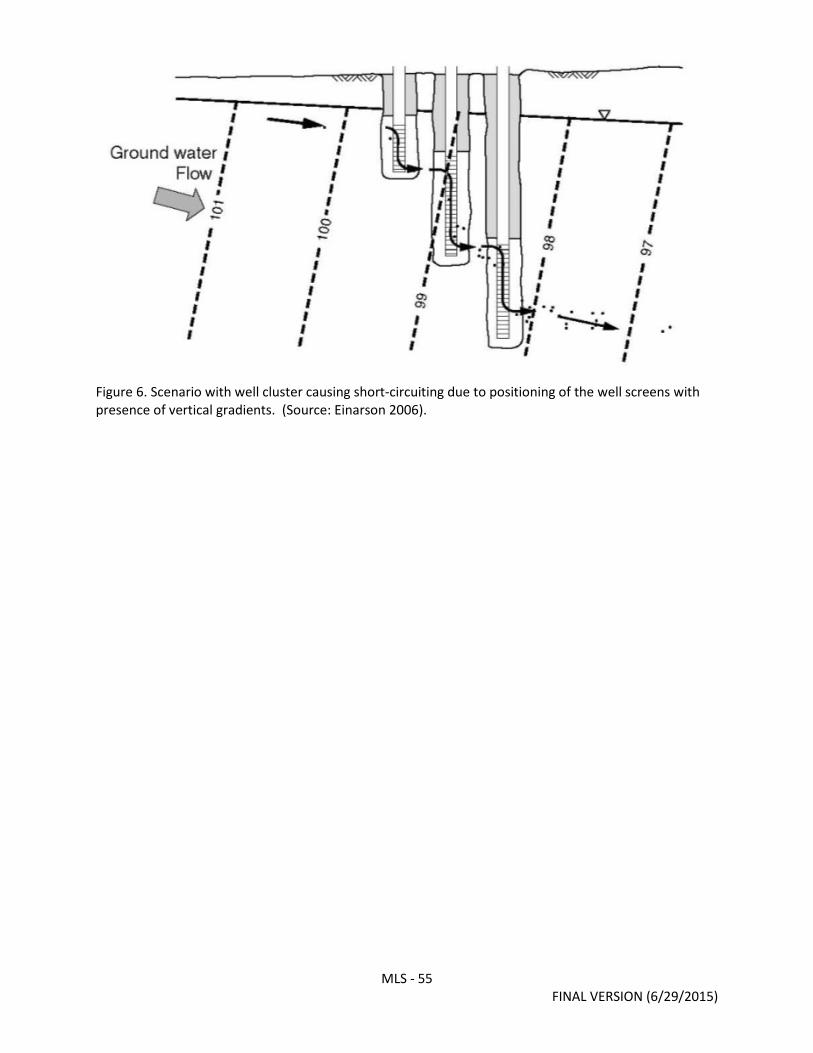
Figure 6. Scenario with well cluster causing short-circuiting due to positioning of the well screens with presence of vertical gradients. (Source: Einarson 2006).
MLS - 55 FINAL VERSION (6/29/2015)

Figure 7. Schematics of generic MLS installation approaches: (a) backfilled system with sand packs around the monitoring intervals and bentonite seals between sand packs (unconsolidated or rock); (b) system in open rock walled hole with packers between open intervals, (c) system installed inside multi-screen casing with packers (adapted from Einarson, 2006), and (d) system in hole fully sealed with a flexible liner, with monitoring intervals formed of a permeable mesh.
MLS - 56 FINAL VERSION (6/29/2015)

Figure 8. Schematic of Solinst CMT system (Source: Einarson 2006).
MLS - 57 FINAL VERSION (6/29/2015)

Figure 9. CMT system (a) CMT tubing, (b) typical CMT intake port, and (c) CMT tubing coil (Source: Einarson and Cherry, 2002).
MLS - 58 FINAL VERSION (6/29/2015)
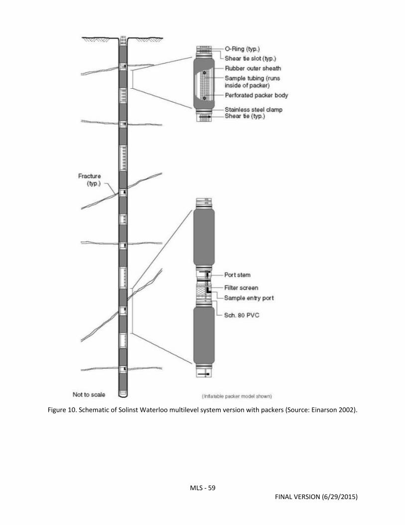
Figure 10. Schematic of Solinst Waterloo multilevel system version with packers (Source: Einarson 2002).
MLS - 59 FINAL VERSION (6/29/2015)
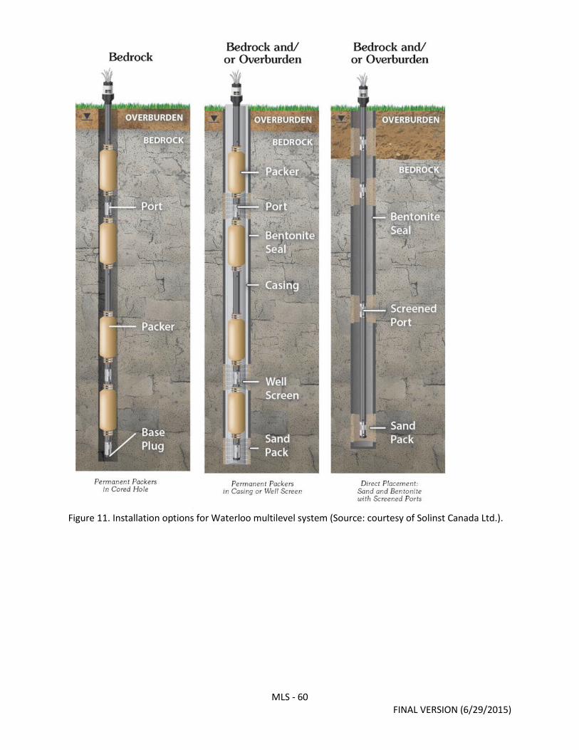
Figure 11. Installation options for Waterloo multilevel system (Source: courtesy of Solinst Canada Ltd.).
MLS - 60 FINAL VERSION (6/29/2015)

Figure 12. Schematic of modified Waterloo System with fifteen ports for installation in sonic casing (Source: Parker et al., 2006).
MLS - 61 FINAL VERSION (6/29/2015)

Figure 13. Schematic of Hybrid Waterloo System with up to nine internal ports and two external piezometers for installation in 6-in tricone holes or 5-in PQ-cored holes (Source: Chapman et al., 2015).
MLS - 62 FINAL VERSION (6/29/2015)

Figure 14. Schematic of (a) FLUTe liner installation procedure with liner attachment to casing, water addition and liner descent below water table, and (b) example (1 port) Water FLUTe groundwater sampling.
MLS - 63 FINAL VERSION (6/29/2015)

Figure 15. Water FLUTe system: (a) installing Water FLUTe system down 6-in borehole, and (b) completed installation (Source: courtesy of FLUTe).
MLS - 64 FINAL VERSION (6/29/2015)

Figure 16. Three Water FLUTe options : (a) the Standard Water FLUTe well-suited for very deep to shallow conditions with positive displacement pumping , (b) the Special Water FLUTe has some compromises to reduce cost, and (c) the Shallow Water FLUTe system is limited to water tables <25 ft below surface with peristaltic pumping at the surface. All the Water FLUTes have head, and transducer measurements.
MLS - 65 FINAL VERSION (6/29/2015)

Figure 17. Schematic of Westbay MP system (Source: courtesy of Westbay).
MLS - 66 FINAL VERSION (6/29/2015)
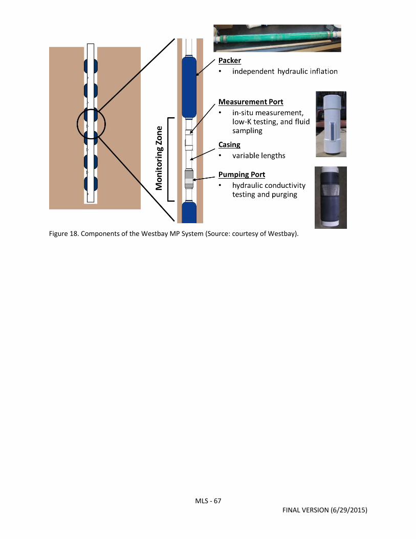
Figure 18. Components of the Westbay MP System (Source: courtesy of Westbay).
MLS - 67 FINAL VERSION (6/29/2015)

Figure 19. Westbay completion options (Source: provided by Westbay Instruments, A Division of Nova Metrix Ground Monitoring (Canada) Ltd.).
MLS - 68 FINAL VERSION (6/29/2015)
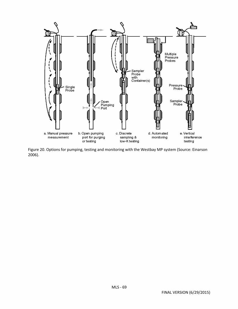
Figure 20. Options for pumping, testing and monitoring with the Westbay MP system (Source: Einarson 2006).
MLS - 69 FINAL VERSION (6/29/2015)
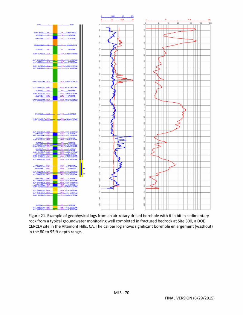
Figure 21. Example of geophysical logs from an air-rotary drilled borehole with 6-in bit in sedimentary rock from a typical groundwater monitoring well completed in fractured bedrock at Site 300, a DOE CERCLA site in the Altamont Hills, CA. The caliper log shows significant borehole enlargement (washout) in the 80 to 95 ft depth range.
MLS - 70 FINAL VERSION (6/29/2015)

Figure 22. Well development considerations based on drilling method and borehole damage.
MLS - 71 FINAL VERSION (6/29/2015)

Figure 23. Example showing well nest design with four separate casings and screens in a single 200 ft deep borehole in Stockton, CA (Source: O’Leary et al., 2012).
MLS - 72 FINAL VERSION (6/29/2015)
APPENDICES APPENDIX A: HISTORY OF DEVELOPMENT OF COMMERCIAL MLSS The Westbay MP system was the first MLS to enter the commercial marketplace for groundwater flow and contamination investigations nearly four decades ago. The development of this system began in Vancouver, BC in the early to mid-1970's by Frank Patton, a geotechnical engineer who formed the Westbay Company there. The earliest system only measured groundwater pressure profiles intended mostly for stability analysis of mountain slopes in British Columbia. The system was adapted for groundwater contamination studies in 1978 when the technology for water sampling was added. This was followed by many improvements in the details of technology over the next two decades. The first large scale use of the Westbay system occurred in thick alluvial aquifer systems in Orange County, CA beginning in the late 1980's (Goodrich and Salden, 1990) where the system was used to create what has become one of the world's most comprehensive groundwater resource monitoring networks that now includes more than 70 systems, each typically about 1,500 feet deep but varying between 500 and 2,000 feet, and with between 10 – 20 monitoring intervals on each system. John Cherry used a prototype version of the Westbay MP system in 1978 for monitoring in sandstone to a depth of 250 m at a prospective uranium mine in Northern Saskatchewan. Soon thereafter, he and a technician (Paul Johnson) at the University of Waterloo began development of prototypes of what became the Waterloo system (Cherry and Johnson, 1982), which several years later became, in a much improved form, the Solinst-Waterloo system marketed by Solinst Canada beginning in 1987. The Waterloo system was developed not to extend the overall capabilities of MLS monitoring, but to provide an alternative that did not require the purchase of specialized downhole tools for data acquisition, and that could easily have dedicated downhole transducers. The Waterloo system has been adapted several times providing configurations suited to a variety of objectives and hydrogeologic settings. Parker et al. (2006) adapted the system to include many more monitoring intervals than previously used and demonstrated installation in sonic drilled holes in overburden and tricone drilled holes in rock. Chapman et al. (2015) later adapted the system to include many monitoring intervals with piezometers attached to the outside of the main MLS casing to allow for transient monitoring of water pressures using small removable transducers and demonstrated installation in tricone rotary drilled holes and in PQ-cored holes. Murray Einarson, who in 1987 had installed several Solinst Waterloo MLSs at a large landfill site in Kern County, California, met John Cherry in that year, which led to a long lasting dialog about MLS technologies and needs for alternative systems. In 1999, Einarson, based in California, invented the CMT system for which prototype testing was done at the Borden experimental site, Ontario, Canada and at Alameda Naval Air Station, California, as part of a University of Waterloo MSc thesis research project, reported on by Einarson and Cherry (2002). The CMT system was not developed to replace the Westbay or Waterloo systems, but rather to fill a different niche, which was to provide an engineered system to replace use of the bundle wells (bundled polyethylene tubes) described by Cherry et al. (1983) for monitoring in unconsolidated deposits. The bundle wells performed satisfactorily in cohesionless sand aquifers that collapsed tightly around the bundle well when the casing used for installation was retracted, but had much uncertainty concerning leakage along the tubes when installed in less cohesive or layered deposits. The CMT system derived advantage from the arrival of widespread availability of rotosonic / sonic drill rigs, which are exceptionally well suited for installation of CMTs. The precursor to the Water FLUTe™ system was invented in the late 1980's by Carl Keller using flexible impervious nylon borehole liners, while Keller was working in New Mexico as a research physicist at
MLS - 73 FINAL VERSION (6/29/2015)

Science and Engineering Associates. Initially this was used only for water and pore gas sampling in the vadose zone in New Mexico, where the vadose zone is commonly a few hundred feet thick. This system was marketed in the early 1990's as the Seamist system. Keller converted it beginning in the mid-1990's to a groundwater sampling and head measurement system known as the Water FLUTe™, manufactured and sold by Flexible Liner Underground Technologies (FLUTe™). Testing of the earliest commercial versions was done in 1997-1998 by the U.S. Army Corps of Engineers at sites in Pennsylvania and California. A simple version of the system with only pressure transducers attached to a liner was used in rock boreholes on the bottom of the Hudson River in 1998. An advanced versions of the WaterFLUTe were tested by the University of Waterloo in Ontario, Canada, beginning in 2000 (Cherry et al., 2007), including the first demonstration of a 15 port Water FLUTe with dedicated pumps and transducers installed in a 5 inch-diameter, dolostone hole in Cambridge, ON and then removed after a year of use to test the removability. The first large commercial order for many Water FLUTes was placed at the Santa Susana Field Laboratory, CA, in 2002. This WaterFLUTe was not developed to replace the other MLSs, but to offer different capabilities that extends the range of MLS use. This system is very different from all other systems. The flexible liner seals the borehole and carries the monitoring systems into place. This system avoids use of packers or bentonite / grout seals between the monitoring intervals because the continuous water-inflated liner forms the seal. The Water FLUTe™ flexible liner systems are easily removable, which facilitates decommissioning the hole or allows the hole to be used for other purposes. Although MLS technologies have improved greatly in capabilities and versatility over the past three decades, and have seen use on nearly all continents serving many different types of groundwater investigations, there is substantial work in progress aimed at extension of the capabilities and robustness as new types of applications are recognized.
MLS - 74 FINAL VERSION (6/29/2015)

LLNL‐TR‐669645 Esser et al. (2015)
278 Recommendations for Groundwater Monitoring Criteria under SB4
12 REFERENCES Alger R. P. (1966) Interpretation of electric logs in fresh water wells in unconsolidated
formations. In Transactions, Society of Professional Well Log Analysts, 7th Annual Logging Symposium (Tulsa, Oklahoma, May 1966). American Petroleum Institute, RP 4S. pp. CC1–CC25.
Allan M. E., Gold D. K. and Reese D. W. (2010) Development of the Belridge Field’s Diatomite Reservoirs With Hydraulically Fractured Horizontal Wells: From First Attempts to Current Ultra‐Tight Spacing. In Society of Petroleum Engineers. Available at: http://www.onepetro.org/doi/10.2118/133511‐MS [Accessed June 19, 2015].
Allan M., Rahman M. and Rycerksi B. (2006) Belridge Giant Oil Field, Diatomite Pool: Learnings from an Unusual Marine Reservoir in an Old Field. In AAPG National Convention (Houston, TX; April 11, 2006). p. Search and Discovery Article #20043. Available at: http://www.searchanddiscovery.com/documents/2006/06143allan/index.htm.
Alley B., Beebe A., Rodgers J. and Castle J. W. (2011) Chemical and physical characterization of produced waters from conventional and unconventional fossil fuel resources. Chemosphere 85, 74–82.
Archie G. E. (1942) The electrical resistivity log as an aid in determining some reservoir characteristics. Am. Inst. Min. Metall. Eng. Trans. 146, 54–62.
Baldassare F. J., McCaffrey M. A. and Harper J. A. (2014) A geochemical context for stray gas investigations in the northern Appalachian Basin: Implications of analyses of natural gases from Neogene‐through Devonian‐age strata. AAPG Bull. 98, 341–372. Available at: http://archives.datapages.com/data/bulletns/2014/02feb/BLTN12178/BLTN12178.HTM [Accessed August 4, 2014].
Ballentine C. J. and Burnard P. G. (2002) Production, release and transport of noble gases in the continental crust. In Noble Gases in Geochemistry and Cosmochemistry Reviews in Mineralogy & Geochemistry. Mineralogical Soc America, Washington. pp. 481–538. Available at: ://000180939700012.
Ballentine C. J., O’Nions R. K., Oxburgh E. R., Horvath F. and Deak J. (1991) Rare gas constraints on hydrocarbon accumulation, crustal degassing and groundwater flow in the Pannonian Basin. Earth Planet. Sci. Lett. 105, 229–246.
Barbot E., Vidic N. S., Gregory K. B. and Vidic R. D. (2013) Spatial and Temporal Correlation of Water Quality Parameters of Produced Waters from Devonian‐Age Shale following Hydraulic Fracturing. Environ. Sci. Technol. 47, 2562–2569.

Esser et al. (2015) LLNL‐TR‐669645
Recommendations for Model Groundwater Monitoring Criteria under SB4 279
Blauch M. E., Myers R. R., Moore T., Lipinski B. A. and Houston N. A. (2009) Marcellus Shale Post‐Frac Flowback Waters ‐ Where is All the Salt Coming from and What are the Implications? In Society of Petroleum Engineers. Available at: http://www.onepetro.org/doi/10.2118/125740‐MS [Accessed April 21, 2015].
Blonde M. S., Gans K. D., Thordsen J. J., Reidy M. E., Thomas B., Engle M. A. and Rowan E. L. (2014) U.S. Geological Survey National Produced Waters Geochemical Database v2.0., U.S. Geological Survey. Available at: http://energy.usgs.gov/EnvironmentalAspects/EnvironmentalAspectsofEnergyProductionandUse/ProducedWaters.aspx#3822349‐data.
Boeken R. (1995) Estimate of water quality in the Dakota aquifer of northwest Kansas using self potential readings of downhole geophysical logs., Kansas Geological Survey Open File Report 95‐1a. Available at: http://www.kgs.ku.edu/Hydro/Publications/1995/OFR95_1a/index.html.
Bohlen S. and Bishop J. (2015) Class II Oil and Gas Underground Injection Control. Division of Oil, Gas, and Geothermal Resources., Letter to Jane Diamond, Water Division Director, Region IX, U.S. Environmental Protection Agency. Available at: ftp://ftp.consrv.ca.gov/pub/oil/UIC%20Files/FINAL_Dual%20Letterhead_US%20EPA%20Letter.pdf.
Boles J. R., Horner S. and Garven G. (2010) Fault/fracture permeability estimated from response of a natural marine methane seep to underlying hydrocarbon production. AAPG Search Discov. Article #40505. Available at: http://www.searchanddiscovery.com/documents/2010/40505boles/ndx_boles.pdf.
Bourgoyne Jr A. T., Scott S. L. and Manowski W. (2000) A Review of Sustained Casing Pressure Occurring on the OCS, final report submitted to., US Department of Interior Minerals Management Service, Washington, D.C.
Boyer E., Swistock B., Clark J., Madden M. and Rizzo D. (2011) The Impact of Marcellus Gas Drilling on Rural Drinking Water Supplies., The Center for Rural Pennsylvania. Available at: http://www.rural.palegislature.us/documents/reports/Marcellus_and_drinking_water_2011_rev.pdf.
Brantley S. L., Yoxtheimer D., Arjmand S., Grieve P., Vidic R., Pollak J., Llewellyn G. T., Abad J. and Simon C. (2014) Water Resource Impacts during Unconventional Shale Gas Development: The Pennsylvania Experience. Int. J. Coal Geol. 126, 140–156.
Brufatto C., Cochran J., Power L. C. D., El‐Zegahty S. Z. A. A., Fraboulet B., Griffin T., James S., Munk T., Justus F., Levine J. R., Montgomery C., Murphy D., Pheiffer J., Pompoch T. and Rishmani L. (2003) Brufatto C, Cochran J, Power LCD, El‐Zeghaty SZAA, Fraboulet B, Griffin T, James S, Munk T, Justus F, Levine JR, Montgomery C, Murphy D, Pfeiffer J,
LLNL‐TR‐669645 Esser et al. (2015)
280 Recommendations for Groundwater Monitoring Criteria under SB4
Pornpoch T, Rishmani L. 2003. From mud to cement ‐ building gas wells. Oilfield Review 15:62‐76. Oilfield Rev. 15, 62–76.
California CVRWQCB (2013a) Aera sump closure in N. Belridge., California Central Valley Regional Water Quality Control Board (Region 5), Order R5‐2013‐0054. Available at: http://www.waterboards.ca.gov/centralvalley/board_decisions/adopted_orders/kern/r5‐2013‐0054.pdf.
California CVRWQCB (2015) California Water Code Directive Pursuant To Section 1326., Central Valley Regional Water Quality Control Board. Available at: http://www.swrcb.ca.gov/centralvalley/water_issues/oil_fields/information/disposal_ponds/ [Accessed June 23, 2015].
California CVRWQCB (2013b) Chevron sump closure., California Central Valley Regional Water Quality Control Board (Region 5), Order R5‐2013‐0056. Available at: http://www.waterboards.ca.gov/centralvalley/board_decisions/adopted_orders/kern/r5‐2013‐0056.pdf.
California CVRWQCB (2012) Waste Discharge Requirements for Chevron USA, Inc., and Cawelo Water District, Produced Water Reclamation Project, Kern River Area Station 36, Kern River Oil Field, Kern County., Central Valley Regional Water Quality Control Board. Available at: http://www.waterboards.ca.gov/centralvalley/board_decisions/adopted_orders/kern/r5‐2012‐0058.pdf.
California CVRWQCB (2004) Water Quality Control Plan for the Tulare Lake Basin, Second Edition., Central Valley Regional Water Quality Control Board. Available at: http://www.waterboards.ca.gov/centralvalley/water_issues/basin_plans/tlbp.pdf.
California DOC and Aspen Environmental Group (2015) Draft Environmental Impact Report: Analysis of Oil and Gas Well Stimulation Treatments in California., California Department of Conservation, State Clearinghouse No. 2013112046. Available at: http://www.conservation.ca.gov/dog/SB4DEIR/Pages/SB4_DEIR_TOC.aspx.
California DOGGR (2015) California DOGGR seeks end to injection in Kern, Tulare County wells., California Division of Oil, Gas & Geothermal Resources. Available at: http://www.conservation.ca.gov/index/news/Documents/2015‐03%20Division%20of%20Oil,%20Gas,%20and%20Geothermal%20Resources%20orders%20UIC%20wells%20shut%20in.pdf.
California DOGGR (1998) California Oil and Gas Fields: Volume 1—Central California., California Division of Oil, Gas and Geothermal Resources. Available at: ftp://ftp.consrv.ca.gov/pub/oil/publications/Datasheets/Dtasheet_vol_1.pdf.
Esser et al. (2015) LLNL‐TR‐669645
Recommendations for Model Groundwater Monitoring Criteria under SB4 281
California DOGGR (2013) Narrative Description of Well Stimulation Draft Regulations., California Division of Oil, Gas & Geothermal Resources. Available at: http://www.conservation.ca.gov/index/Documents/Narrative Description of Well Stimulation Draft Regulations 20131114 final.pdf.
California SWRCB (1988) Sources of Drinking Water Policy, Resolution No 88‐63., California State Water Resources Control Board. Available at: http://www.swrcb.ca.gov/board_decisions/adopted_orders/resolutions/2006/rs2006_0008_rev_rs88_63.pdf.
California SWRCB (2014) Underground Injection Control Drinking Water Source Evaluation., California State Water Resources Control Board, Letter to EPA Region 9 Administrator Jared Blumenfeld. Available at: http://www.biologicaldiversity.org/campaigns/california_fracking/pdfs/20140915_Bishop_letter_to_Blumenfeld_Responding_to_July_17_2014_UIC_Letter.pdf.
Cardno ENTRIX (2012) Hydraulic Fracturing Study, PXP Inglewood Oil Field., Plains Exploration & Production Company and Los Angeles County, Department of Regional Planning, Los Angeles, CA. Available at: http://www.scribd.com/doc/109624423/Hydraulic‐Fracturing‐Study‐Inglewood‐Field10102012.
Carey J. W., Lewis K., Kelkar S. and Zyvoloski G. A. (2013) Geomechanical Behavior of Wells in Geologic Sequestration. Energy Procedia 37, 5642–5652.
Carpenter A. B. and Moore T. S. (1997) Origin of Boron‐Rich Pore Water in the Monterey Formation, San Joaquin Valley, CA CARPENTER, ALDEN B., and TRACEY S. MOORE. In Search and Discovery Article #90945 (AAPG Pacific Section Meeting; Bakersfield, California; 1997). Available at: http://www.searchanddiscovery.com/abstracts/html/1997/pacific/abstracts/0681d.htm.
CCA (2014) Environmental Impacts of Shale Gas Extraction in Canada., Council of Canadian Academies: The Expert Panel on Harnessing Science and Technology to Understand the Environmental Impacts of Shale Gas Extraction. Available at: http://www.scienceadvice.ca/en/assessments/completed/shale‐gas.aspx.
CCA and Cherry J. A. (2014) Environmental Impacts of Shale Gas Extraction in Canada., Council of Canadian Academies: The Expert Panel on Harnessing Science and Technology to Understand the Environmental Impacts of Shale Gas Extraction. Available at: http://www.scienceadvice.ca/en/assessments/completed/shale‐gas.aspx.
CCST, LBNL and Pacific Institute (2014) Advanced Well Stimulation Technologies in California: An Independent Review of Scientific and Technical Information., California Council on Science and Technology, Lawrence Berkeley National Laboratory, and Pacific Institute. Available at: http://www.ccst.us/projects/fracking_public/BLM.php.

LLNL‐TR‐669645 Esser et al. (2015)
282 Recommendations for Groundwater Monitoring Criteria under SB4
Chapman E. C., Capo R. C., Stewart B. W., Kirby C. S., Hammack R. W., Schroeder K. T. and Edenborn H. M. (2012) Geochemical and Strontium Isotope Characterization of Produced Waters from Marcellus Shale Natural Gas Extraction. Environ. Sci. Technol. 46, 3545–3553.
Cherry J. A., Parker B. L., Bradbury K. R., Eaton T. T., Gotkowitz M. B., Hart D. J. and Borchardt M. A. (2006) Contaminant Transport Through Aquitards: A State‐of‐the‐Science Review., Awwa Research Foundation Report 91133a. Available at: http://www.waterrf.org/PublicReportLibrary/91133a.pdf.
Chilingar G. V. and Endres B. (2005) Environmental hazards posed by the Los Angeles Basin urban oilfields: an historical perspective of lessons learned. Environ. Geol. 47, 302–317.
Coats K. H. (1987) Reservoir Simulation (Chapter 48). In Petroleum Engineering Handbook (Howard B. Bradley, ed.) Society of Petroleum Engineers. Available at: https://www.onepetro.org/book/peh/spe‐1987‐48‐peh [Accessed June 29, 2015].
Crumbling D. M. (2004) Summary of the Triad approach., U.S. Environmental Protection Agency Office of Superfund Remediation and Technology Innovation. Available at: http://www.triadcentral.org/ref/ref/index.cfm.
Darrah T. H., Jackson R. B., Poreda R. J., Warner N. R. and Vengosh A. (2014) The source and migration of natural gas in shallow aquifers: Insights provided by the integration of noble gas and hydrocarbon isotopes (abstr.). In Goldschmidt 2014 (Sacramento, California; June 8‐13, 2014). Available at: http://goldschmidt.info/2014/program.
Darrah T. H., Jackson R. B., Vengosh A., Warner N. R. and Poreda R. J. (2015) Noble Gases: A new technique for fugitive gas investigation in groundwater. Groundwater 53, 19–28.
Darrah T. H., Vengosh A., Jackson R. B., Warner N. R. and Poreda R. J. (2014) Noble gases identify the mechanisms of fugitive gas contamination in drinking‐water wells overlying the Marcellus and Barnett Shales. Proc. Natl. Acad. Sci. 111, 14076–14081.
Davies R. J. (2011) Methane contamination of drinking water caused by hydraulic fracturing remains unproven. Proc. Natl. Acad. Sci. U. S. A. 108, E871–E871.
Davies R. J., Almond S., Ward R. S., Jackson R. B., Adams C., Worrall F., Herringshaw L. G., Gluyas J. G. and Whitehead M. A. (2014) Oil and gas wells and their integrity: Implications for shale and unconventional resource exploitation. Mar. Pet. Geol. 56, 239–254.
Davies R. J., Mathias S. a., Moss J., Hustoft S. and Newport L. (2012) Hydraulic fractures: How far can they go? Mar. Pet. Geol. 37, 1–6.
DiGiulio D. C., Wilkin R. T., Miller C. and Oberley G. (2011) Investigation of Ground Water Contamination near Pavillion, Wyoming., US Environmental Protection Agency (Office of Research and Development, National Risk Management Research Laboratory) EPA

Esser et al. (2015) LLNL‐TR‐669645
Recommendations for Model Groundwater Monitoring Criteria under SB4 283
600/R‐00/000. Available at: www.epa.gov/ord http://www2.epa.gov/region8/pavillion http://www2.epa.gov/region8/investigation‐ground‐water‐contamination‐near‐pavillion‐wyoming‐workgroup‐meeting‐november.
Dusseault M. B., Bruno M. S. and Barrera J. (2001) Casing shear: causes, cases, cures. SPE Drill. Complet. 16, 98–107.
Dusseault M. B., Gray M. N. and Nawrocki P. A. (2000) Why Oilwells Leak : Cement Behavior and Long‐Term Consequences. In SPE International Oil and Gas Conference and Exhibition, SPE 64733 Society of Petroleum Engineers, Beijing, China. p. 8.
Eichhubl P. and Boles J. R. (2000) Focused fluid flow along faults in the Monterey Formation, coastal California. Geol. Soc. Am. Bull. 112, 1667–1679.
Emanuele M., Minner W. A., Broussard E. J., Blevens D. M. and Taylor B. T. (1998) A Case History: Completion and Stimulation of Horizontal Wells with Multiple Transverse Hydraulic Fractures in the Lost Hills Diatomite. In Proceedings of SPE Rocky Mountain Regional/Low‐Permeability Reservoirs Symposium (Denver, CO, 5‐8 April, 1998). p. SPE–39941–MS.
Engelder T. (2012) Capillary tension and imbibition sequester frack fluid in Marcellus gas shale. Proc. Natl. Acad. Sci. U. S. A. 109, E3625; author reply E3626.
ERCB (2012) Caltex Energy Inc. Hydraulic Fracturing Incident 16‐27‐068‐10W6M September 22, 2011 ERCB Investigation Report (Released: December 20, 2012).
Faunt C. C. (2009) Groundwater Availability of the Central Valley Aquifer, California., U.S. Geological Survey Professional Paper 1766. Available at: http://ca.water.usgs.gov/projects/central‐valley/central‐valley‐hydrologic‐model.html.
Ferrar K. J., Michanowicz D. R., Christen C. L., Mulcahy N., Malone S. L. and Sharma R. K. (2013) Assessment of Effluent Contaminants from Three Facilities Discharging Marcellus Shale Wastewater to Surface Waters in Pennsylvania. Environ. Sci. Technol. 47, 3472–3481.
Fischer M., Foxall W., Jordan P., Lindsey N., Millstein D., Reagan M., Stringfellow W., Tinnacher R., Varadharajan C., Cooley H., Donnelly K., Heberger M. and Feinstein L. (2014) Chapter 5: Potential Direct Environmental Effects of Well Stimulation. In Advanced Well Stimulation Technologies in California: An Independent Review of Scientific and Technical Information. The California Council on Science and Technology (CCST), Lawrence Berkeley National Laboratory (LBNL) and the Pacific Institute,.
Fisher J. B. and Boles J. R. (1990) Water—rock interaction in Tertiary sandstones, San Joaquin basin, California, U.S.A.: Diagenetic controls on water composition. Chem. Geol. 82, 83–101.
LLNL‐TR‐669645 Esser et al. (2015)
284 Recommendations for Groundwater Monitoring Criteria under SB4
Fisher K. and Warpinski N. (2012) Hydraulic‐Fracture‐Height Growth: Real Data. SPE Prod. Oper. 27, 8–19.
Flewelling S. A. and Sharma M. (2014) Constraints on Upward Migration of Hydraulic Fracturing Fluid and Brine. Groundwater 52, 9–19.
Flewelling S. a., Tymchak M. P. and Warpinski N. (2013) Hydraulic fracture height limits and fault interactions in tight oil and gas formations. Geophys. Res. Lett. 40, 3602–3606.
Folger P., Tiemann M. and Bearden D. M. (2012) The EPA Draft Report of Groundwater Contamination Near Pavillion, Wyoming: Main Findings and Stakeholder Responses., Congressional Research Service. Available at: http://wyofile.com/wp‐content/uploads/2012/01/R42327‐2.pdf.
Fontenot B. E., Hunt L. R., Hildenbrand Z. L., Carlton Jr. D. D., Oka H., Walton J. L., Hopkins D., Osorio A., Bjorndal B., Hu Q. H. and Schug K. A. (2013) An Evaluation of Water Quality in Private Drinking Water Wells Near Natural Gas Extraction Sites in the Barnett Shale Formation. Environ. Sci. Technol. 47, 10032–10040.
Foppen J. W., Orup C., Adell R., Poulalion V. and Uhlenbrook S. (2011) Using multiple artificial DNA tracers in hydrology. Hydrol. Process. 25, 3101–3106.
Frankiewicz T. (2015) Produced Water Management in California Oil Fields. In Groundwater Resources Association of California Symposium on Oil, Gas and Groundwater in California (February 19, 2015; Long Beach, CA).
Fredrich J. T., Arguello J. G., Thorne B. J., Wawersik W. R., Deitrick G. L., de Rouffignac E. P., Myer L. R. and Bruno M. S. (1996) Three‐Dimensional Geomechanical Simulation of Reservoir Compaction and Implications for Well Failures in the Belridge Diatomite. In Society of Petroleum Engineers. Available at: http://www.onepetro.org/doi/10.2118/36698‐MS [Accessed June 19, 2015].
Geoscience Analytical I. (1986) A Study of Abandoned Oil and Gas Wells and Methane and Other Hazardous Gas Accumulations., Available at: ftp://ftp.consrv.ca.gov/pub/oil/A Study of Abandoned Oil and Gas Wells and Methane and Other Hazardous Gas Accumulations.pdf.
Golding S. D., Boreham C. J. and Esterle J. S. (2013) Stable isotope geochemistry of coal bed and shale gas and related production waters: A review. Int. J. Coal Geol. 120, 24–40.
Gross S. A., Avens H. J., Banducci A. M., Sahmel J., Panko J. M. and Tvermoes B. E. (2013) Analysis of BTEX groundwater concentrations from surface spills associated with hydraulic fracturing operations. J. Air Waste Manag. Assoc. 63, 424–432.
Guyod H. (1944) Fundamentals of electric log interpretation., Halliburton Company, Welex Division (Houston, Texas).

Esser et al. (2015) LLNL‐TR‐669645
Recommendations for Model Groundwater Monitoring Criteria under SB4 285
GWPC (2012) White Paper Summarizing 2012 Stray Gas Incidence & Response Forum., Ground Water Protection Council.
Haluszczak L. O., Rose A. W. and Kump L. R. (2013) Geochemical evaluation of flowback brine from Marcellus gas wells in Pennsylvania, USA. Appl. Geochem. 28, 55–61.
Hammack R., Harbert W., Sharma S., Stewart B., R. Capo, Wall A., Wells A., Diehl R., Blaushild D., Sams J. and Veloski G. (2014) An Evaluation of Fracture Growth and Gas/Fluid Migration as Horizontal Marcellus Shale Gas Wells are Hydraulically Fractured in Greene County, Pennsylvania., U.S. Department of Energy, National Energy Technology Laboratory NETL‐TRS‐3‐2014. Available at: http://www.netl.doe.gov/File%20Library/Research/onsite%20research/publications/NETL‐TRS‐3‐2014_Greene‐County‐Site_20140915_1_1.pdf.
Harkness J. S., Dwyer G. S., Warner N. R., Parker K. M., Mitch W. A. and Vengosh A. (2015) Iodide, Bromide, and Ammonium in Hydraulic Fracturing and Oil and Gas Wastewaters: Environmental Implications. Environ. Sci. Technol. Available at: http://pubs.acs.org/doi/abs/10.1021/es504654n [Accessed January 14, 2015].
Harrison S. S. (1985) Contamination of Aquifers by Overpressuring the Annulus of Oil and Gas Wells. Ground Water 23, 317–324.
Harrison S. S. (1983) Evaluating System for Ground‐Water Contamination Hazards Due to Gas‐Well Drilling on the Glaciated Appalachian Plateau. Ground Water 21, 689–700.
Hayes T. (2009) Sampling and Analysis of Water Streams Associated with the Development of Marcellus Shale Gas., Marcellus Shale Coalition. Available at: http://energyindepth.org/wp‐content/uploads/marcellus/2012/11/MSCommission‐Report.pdf.
Hejl K. A., Madding A. M., Morea M., Glatz C. W., Luna J. B., Minner W. A., Stanley G. R. and Singh T. (2007) Extreme Multistage Fracturing Improves Vertical Coverage and Well Performance in the Lost Hills Field. SPE Drill. Complet. 22, 326–333.
Holcomb R. (2015) Oil Field Produced Water Pond Status Report #3 ( Letter to Pamela Creedon, Clay L. Rogers, and Doug Patterson)., Central Valley Regional Water Quality Control Board. Available at: http://www.swrcb.ca.gov/centralvalley/water_issues/oil_fields/information/disposal_ponds/pond_status_rpt3_2015_0404.pdf.
Hosford Scheirer A. (2007) Chapter 7: The Three‐Dimensional Geologic Model Used for the 2003 National Oil and Gas Assessment of the San Joaquin Basin Province, California. In Petroleum Systems and Geologic Assessment of Oil and Gas in the San Joaquin Basin Province, California, U.S. Geological Survey Professional Paper 1713. Available at: http://pubs.usgs.gov/pp/pp1713/.

LLNL‐TR‐669645 Esser et al. (2015)
286 Recommendations for Groundwater Monitoring Criteria under SB4
Hughes J. D. (2013) Drilling California: A Reality Check on the Monterey Shale., Post Carbon Institute and Physicians Scientists & Engineers for Healthy Energy. Available at: http://www.postcarbon.org/reports/Drilling‐California_FINAL.pdf.
Ingraffea A. R., Wells M. T., Santoro R. L. and Shonkoff S. B. C. (2014) Assessment and risk analysis of casing and cement impairment in oil and gas wells in Pennsylvania, 2000–2012. Proc. Natl. Acad. Sci. 111, 10955–10960.
ITRC (2003) Technical and Regulatory Guidance for the Triad Approach: A New Paradigm for Environmental Project Management., Interstate Technology and Regulatory Council SCM‐1. Available at: http://www.itrcweb.org/SCM‐1.pdf.
Jackson R. B. (2014) The integrity of oil and gas wells. Proc. Natl. Acad. Sci. 111, 10902–10903.
Jackson R. B., Vengosh A., Carey J. W., Davies R. J., Darrah T. H., O’Sullivan F. and Pétron G. (2014) The Environmental Costs and Benefits of Fracking. Annu. Rev. Environ. Resour. 39, 327–362.
Jackson R. B., Vengosh A., Darrah T. H., Warner N. R., Down A., Poreda R. J., Osborn S. G., Zhao K. and Karr J. D. (2013) Increased stray gas abundance in a subset of drinking water wells near Marcellus shale gas extraction. Proc. Natl. Acad. Sci. 110, 11250–11255.
Jackson R. E., Gorody A. W., Mayer B., Roy J. W., Ryan M. C. and Van Stempvoort D. R. (2013) Groundwater Protection and Unconventional Gas Extraction: The Critical Need for Field‐Based Hydrogeological Research. Groundwater 51, 488–510.
Jorgensen D. G. (1989) Using geophysical logs to estimate porosity, water resistivity, and intrinsic permeability., U.S. Geological Survey Water Supply Paper 2321. Available at: http://pubs.er.usgs.gov/publication/wsp2321 [Accessed March 30, 2015].
Kargbo D. M., Wilhelm R. G. and Campbell D. J. (2010) Natural Gas Plays in the Marcellus Shale: Challenges and Potential Opportunities. Environ. Sci. Technol. 44, 5679–5684.
Kell S. (2011) State Oil and Gas Agency Groundwater Investigations and Their Role in Advancing Regulatory Reforms ‐ A Two‐State Review: Ohio and Texas., Ground Water Protection Council.
Kharaka Y. K., Hull R. W. and Carothers W. W. (1985) Water‐Rock Interactions in Sedimentary Basins. In In: Relationship of Organic Matter and Mineral Diagenesis (SC17) The Society of Economic Paleontologists and Mineralogists (SEPM). pp. 79–176.
Kim J. and Moridis G. J. (2012) Gas Flow Tightly Coupled to Elastoplastic Geomechanics for Tight and Shale Gas Reservoirs : Material Failure and Enhanced Permeability. In Proc. Americas Unconventional Resources Conference Piitsburgh, PA.

Esser et al. (2015) LLNL‐TR‐669645
Recommendations for Model Groundwater Monitoring Criteria under SB4 287
Kim J., Um E. S. and Moridis G. J. (2014) SPE 168578 Fracture Propagation , Fluid Flow , and Geomechanics of Water‐Based Hydraulic Fracturing in Shale Gas Systems and Electromagnetic Geophysical Monitoring of Fluid Migration. In Proc. SPE Hydraulic Fracturing Technology Conference Woodlands, TX.
King G. (2011) Tracking Fracture Fluid Movement with Chemical and Gamma‐Emitting Tracers with Verification by Microseismic Recording. In Proceedings of the Technical Workshops for the Hydraulic Fracturing Study: Chemical & Analytical Methods U.S. Environmental Protection Agency EPA 600/R‐11/066. pp. 70–73. Available at: http://water.epa.gov/type/groundwater/uic/class2/hydraulicfracturing/hfworkshops.cfm [Accessed March 27, 2015].
King G. E. (2012a) Estimating Frac Risk and Improving Frac Performance in Unconventional Gas and Oil Wells (SPE 152596). In Society of Petroleum Engineers Hydraulic Fracturing Conference (Woodlands, TX. February 2012). Available at: http://www.gekengineering.com/index.html http://gekengineering.com/Downloads/Free_Downloads/Estimating_and_Explaining_Fracture_Risk_and_Improving_Fracture_Performance_in_Unconventional_Gas_and_Oil_Wells.pdf.
King G. E. (2012b) Hydraulic Fracturing 101: What Every Representative, Environmentalist, Regulator, Reporter, Investor, University Researcher, Neighbor and Engineer Should Know About Estimating Frac Risk and Improving Frac Performance in Unconventional Gas and Oil Wells (SPE 152596). In SPE Hydraulic Fracturing Technology Conference (6‐8 February 2012, The Woodlands, TX). Society of Petroleum Engineers. Available at: https://www.onepetro.org/conference‐paper/SPE‐152596‐MS.
King G. E. and King D. E. (2013) Environmental Risk Arising From Well‐Construction Failure‐Differences Between Barrier and Well Failure, and Estimates of Failure frequency Across Common Well Types, Locations, and Well Age. SPSE Prod. Oper. 28, 323–344.
Kissinger A., Helmig R., Ebigbo A., Class H., Lange T., Sauter M., Heitfeld M., Klunker J. and Jahnke W. (2013) Hydraulic fracturing in unconventional gas reservoirs: risks in the geological system, part 2. Environ. Earth Sci. 70, 3855–3873. Available at: ://WOS:000327457600030.
Kolesar Kohl C. A., Capo R. C., Stewart B. W., Wall y, Schroeder K. T., Hammack R. W. and Guthrie G. D. (2014) Strontium Isotopes Test Long‐Term Zonal Isolation of Injected and Marcellus Formation Water after Hydraulic Fracturing. Environ. Sci. Technol. 48, 9867–9873.
Kolodny Y. and Chaussidon M. (2004) Boron isotopes in DSDP cherts: Fractionation and diagenesis. In The Geochemical Society Special Publications (ed. J. L., Zeev Aizenshtat, Mary Jo Baedecker, George Claypool, Robert Eganhouse, Martin Goldhaber and Kenneth Peters Ronald J. Hill). Geochemical Investigations in Earth and Space Science: A Tribute

LLNL‐TR‐669645 Esser et al. (2015)
288 Recommendations for Groundwater Monitoring Criteria under SB4
to Isaac R. Kaplan. Elsevier. pp. 1–14. Available at: http://www.sciencedirect.com/science/article/pii/S1873988104800038 [Accessed March 22, 2015].
Kornacki A. S. and McCaffrey M. A. (2011) Applying geochemical fingerprinting technology to determine the source of natural gas samples obtained from water wells in Parker County and Hood County, Texas., Weatherford Laboratories (Houston, Texas).
Kresse T. M., Warner N. R., Hayes P. D., Down A., Vengosh A. and Jackson R. B. (2012) Shallow groundwater quality and geochemistry in the Fayetteville Shale gas‐production area, north‐central Arkansas, 2011., U.S. Geological Survey Scientific Investigations Report 2012‐5273. Available at: http://pubs.usgs.gov/sir/2012/5273/.
Llewellyn G. T., Dorman F., Westland J. L., Yoxtheimer D., Grieve P., Sowers T., Humston‐Fulmer E. and Brantley S. L. (2015) Evaluating a groundwater supply contamination incident attributed to Marcellus Shale gas development. Proc. Natl. Acad. Sci. 112, 6325–6330.
Lollar B. S. and Ballentine C. J. (2009) Insights into deep carbon derived from noble gases. Nat. Geosci. 2, 543–547.
Long J. C. S., Feinstein L. C., Birkholzer J., Jordan P., Houseworth J., Dobson P. F., Heberger M. and Gautier D. L. (2015) An Independent Scientific Assessment of Well Stimulation in California, Volume I: Well Stimulation Technologies and their Past, Present, and Potential Future Use in California., California Council on Science and Technology and Lawrence Berkeley National Laboratory. Available at: http://ccst.us/projects/hydraulic_fracturing_public/SB4.php.
Maguire‐Boyle S. J. and Barron A. R. (2014) Organic compounds in produced waters from shale gas wells. Environ. Sci. Process. Impacts. Available at: http://pubs.rsc.org/en/content/articlelanding/2014/em/c4em00376d [Accessed September 9, 2014].
McMahon P. B., Caldwell R., Galloway J. M., Valder J. F. and Hunt A. G. (2015) Quality and Age of Shallow Groundwater in the Bakken Formation Production Area, Williston Basin, Montana and North Dakota. Groundwater 53, 81–94.
Molofsky L. J., Connor J. A., Wylie A. S., Wagner T. and Farhat S. K. (2013a) Evaluation of Methane Sources in Groundwater in Northeastern Pennsylvania. Groundwater 51, 333–349. Available at: http://onlinelibrary.wiley.com/doi/10.1111/gwat.12056/abstract [Accessed August 19, 2014].
Molofsky L. J., Connor J. A., Wylie A. S., Wagner T. and Farhat S. K. (2013b) Evaluation of Methane Sources in Groundwater in Northeastern Pennsylvania. Groundwater 51, 333–349.
Esser et al. (2015) LLNL‐TR‐669645
Recommendations for Model Groundwater Monitoring Criteria under SB4 289
Molofsky L. J., Connor J. A., Wylie A. S., Wagner T. and Farhat S. K. (2013c) Evaluation of Methane Sources in Groundwater in Northeastern Pennsylvania. Groundwater 51, 333–349.
Muehlenbachs K. (2012) Muehlenbachs, K. (2013) Identifying the Sources of Fugitive Methane Associated with Shale Gas Development, Resources For the Future, Washington, DC. In Managing the risks of shale gas: Identifying a pathway toward responsible development (November 14, 2011; Resources For the Future, Washington, DC.). Available at: http://www.rff.org/Events/Pages/Managing‐the‐Risks‐of‐Shale‐Gas.aspx.
NYDEC (2011) Revised Draft Supplemental Generic Environmental Impact Statement on the Oil, Gas and Solution Mining Regulatory Program, Well Permit Issuance for Horizontal Drilling And High‐Volume Hydraulic Fracturing in the Marcellus Shale and Other Low‐Permeability Gas Reservoirs. New York State Department of Environmental Conservation., New York State Department of Environmental Conservation, Albany, NY. Available at: http://www.dec.ny.gov/energy/75370.html.
Onions R. and Ballentine C. (1993) Rare‐Gas Studies of Basin‐Scale Fluid Movement. Philos. Trans. R. Soc. Lond. Ser. ‐Math. Phys. Eng. Sci. 344, 141–156.
Osborn S. G., Vengosh A., Warner N. R. and Jackson R. B. (2011) Methane contamination of drinking water accompanying gas‐well drilling and hydraulic fracturing. Proc. Natl. Acad. Sci. U. S. A. 108, 8172–8176.
Page R. W. (1973) Base of fresh ground water (approximately 3,000 micromhos) in the San Joaquin Valley, California., U.S. Geological Survey Hydrologic Atlas 489. Available at: http://pubs.er.usgs.gov/publication/ha489 [Accessed March 30, 2015].
Papoulias D. M. and Velasco A. L. (2013) Histopathological Analysis of Fish from Acorn Fork Creek, Kentucky, Exposed to Hydraulic Fracturing Fluid Releases. Southeast. Nat. 12, 92–111.
Parker K. M., Zeng T., Harkness J., Vengosh A. and Mitch W. A. (2014) Enhanced Formation of Disinfection Byproducts in Shale Gas Wastewater‐Impacted Drinking Water Supplies. Environ. Sci. Technol. 48, 11161–11169.
Pennsylvania DEP (2009a) DEP Fines Cabot Oil and Gas Corp. $56,650 for Susquehanna County Spills., Pennsylvania Department of Environmental Protection, Williamsport, PA. Available at: http://www.portal.state.pa.us/portal/server.pt/community/newsroom/14287?id=2399&typeid=1.
Pennsylvania DEP (2009b) Inspection Report., Commonwealth of Pennsylvania Department of Environmental Protection. Available at: http://www.marcellus‐shale.us/pdf/CC‐Spill_DEP‐Insp‐Rpt.pdf [Accessed June 25, 2014].

LLNL‐TR‐669645 Esser et al. (2015)
290 Recommendations for Groundwater Monitoring Criteria under SB4
Planert M. and Williams J. S. (1995) Groundwater Atlas of the United States: California, Nevada by Michael Planert and John S. Williams., U.S. Geological Survey HA 730‐B. Available at: http://pubs.usgs.gov/ha/ha730/ch_b/index.html.
Quinn N. H., Wainwright H., Jordan P., Zhou Q. and Birkholzer J. (2013) Potential Impacts of Future Geological Storage of CO2 on the Groundwater Resources in California’s Central Valley: Simulations Of Deep Basin Pressure Changes And Effect On Shallow Water Resources., Caliifornia Energy Commission Report CEC‐500‐2014‐028. Available at: http://www.energy.ca.gov/2014publications/CEC‐500‐2014‐028/CEC‐500‐2014‐028.pdf.
Revkin A. C. (2013) Ideas to Watch in 2013: Traceable Gas‐Drilling Fluids (Dot Earth Blog, January 8th, 2013). N. Y. Times. Available at: http://dotearth.blogs.nytimes.com/2013/01/08/ideas‐to‐watch‐in‐2013‐traceable‐frackin‐fluids/ [Accessed March 30, 2015].
Ritter S. K. (2014) A New Way Of Fracking. Chem. Eng. News 92, 31–33.
De Rouffignac E. P., Bondor P. L., Karanikas J. M. and Hara S. K. (1995) Subsidence and Well Failure in the South Belridge Diatomite Field. In Society of Petroleum Engineers. Available at: http://www.onepetro.org/doi/10.2118/29626‐MS [Accessed June 19, 2015].
Rowan E. L., Engle M. A., Kraemer T. F., Schroeder K. T., Hammack R. W. and Doughten M. W. (2015) Geochemical and isotopic evolution of water produced from Middle Devonian Marcellus shale gas wells, Appalachian basin, Pennsylvania. Aapg Bull. 99, 181–206.
Rozell D. J. and Reaven S. J. (2012) Water Pollution Risk Associated with Natural Gas Extraction from the Marcellus Shale. Risk Anal. 32, 1382–1393.
Rutqvist J., Rinaldi A. P., Cappa F. and Moridis G. J. (2013) Modeling of fault reactivation and induced seismicity during hydraulic fracturing of shale‐gas reservoirs. J. Pet. Sci. Eng. 107, 31–44.
Sabir I. H., Torgersen J., Haldorsen S. and Aleström P. (1999) DNA tracers with information capacity and high detection sensitivity tested in groundwater studies. Hydrogeol. J. 7, 264–272.
Schlumberger (1997) Log Interpretation Charts., Schlumberger (Houston, Texas).
Schmitt S. J., Dawson B. J. M. and Belitz K. (2009) Groundwater‐quality data in the Antelope Valley study unit, 2008: Results from the California GAMA program., U.S. Geological Survey Data Series 479. Available at: http://pubs.usgs.gov/ds/479/.
Schmitt S. J., Fram M. S., Dawson B. J. M. and Belitz K. (2008) Ground‐Water Quality Data in the Middle Sacramento Valley Study Unit, 2006—Results from the California GAMA

Esser et al. (2015) LLNL‐TR‐669645
Recommendations for Model Groundwater Monitoring Criteria under SB4 291
Program., U.S. Geological Survey Data Series 385. Available at: http://ca.water.usgs.gov/gama/SU/cen_sacto.htm.
Schon S. C. (2011) Hydraulic fracturing not responsible for methane migration. Proc. Natl. Acad. Sci. U. S. A. 108, E664–E664.
Serres‐Piole C., Preud’homme H., Moradi‐Tehrani N., Allanic C., Jullia H. and Lobinski R. (2012) Water tracers in oilfield applications: Guidelines. J. Pet. Sci. Eng. 98–99, 22–39.
Siegel D. I., Azzolina N. A., Smith B. J., Perry A. E. and Bothun R. L. (2015) Methane Concentrations in Water Wells Unrelated to Proximity to Existing Oil and Gas Wells in Northeastern Pennsylvania. Environ. Sci. Technol. Available at: http://dx.doi.org/10.1021/es505775c [Accessed April 1, 2015].
Van Stempvoort D., Maathuis H., Jaworski E., Mayer B. and Rich K. (2005) Oxidation of fugitive methane in ground water linked to bacterial sulfate reduction. Ground Water 43, 187–199.
Stepan D. J., Shockey R. E., Kurz B. A., Kalenze N. S., Cowan R. M., Ziman J. J. and Harju J. A. (2010) Bakken Water Opportunities Assessment—Phase I., Energy and Environmental Research Center (University of North Dakota) 2010‐EERC‐04‐03.
Stringfellow W. T., Cooley H., Varadharajan C., Heberger M., Reagan M., Domen J. K., Sandelin W., Camarillo M. K., Jordan P., Donnelly K., Nicklisch S., Hamdoun A. and Houseworth J. (2015) Chapter 2: Impacts of Well Stimulation on Water Resources. In An Independent Scientific Assessment of Well Stimulation in California, Volume II: Generic and Potential Environmental Impacts of Well Stimulation Treatments, Chapter 2 California Council on Science and Technology, Lawrence Berkeley National Laboratory, and the Pacific Institute. Available at: http://ccst.us/projects/hydraulic_fracturing_public/SB4.php.
Stringfellow W. T., Domen J. K., Camarillo M. K., Sandelin W. L. and Borglin S. (2014) Physical, chemical, and biological characteristics of compounds used in hydraulic fracturing. J. Hazard. Mater. 275, 37–54.
Taylor K. A., Fram M. S., Landon M. K., Kulongoski J. T. and Faunt C. C. (2014) Oil, Gas, and Groundwater in California ‐ a discussion of issues relevant to monitoring the effects of well stimulation at regional scales., California Water Science Center, U.S. Geological Survey. Prepared in cooperation with the California State Water Resources Control Board. Available at: http://www.waterboards.ca.gov/water_issues/programs/groundwater/sb4/index.shtml.
Tixier M. P. (1949) Evaluation of permeability from electric log resistivity gradients. Oil Gas J., 113.

LLNL‐TR‐669645 Esser et al. (2015)
292 Recommendations for Groundwater Monitoring Criteria under SB4
Townend J. and Zoback M. D. (2004) Regional tectonic stress near the San Andreas fault in central and southern California. Geophys. Res. Lett. 31, L15S11.
USEPA (2015a) Analysis of Hydraulic Fracturing Fluid Data from the FracFocus Chemical Disclosure Registry 1.0., U.S. Environmental Protection Agency Office of Research and Development EPA/601/R‐14/003, Washington, D.C. Available at: http://www2.epa.gov/hfstudy/epa‐analysis‐fracfocus‐1‐data.
USEPA (2015b) Assessment of the Potential Impacts of Hydraulic Fracturing for Oil and Gas on Drinking Water Resources (External Review Draft)., US Environmental Protection Agency National Center for Environmental Assessment. Available at: http://cfpub.epa.gov/ncea/hfstudy/recordisplay.cfm?deid=244651 [Accessed June 5, 2015].
USEPA (2014a) Code of Federal Regulations, T., Chapter I, Subchapter N, Part 435, Subpt. A, App. 1, 2014., U.S. Environmental Protection Agency. Available at: http://www.ecfr.gov/cgi‐bin/text‐idx?SID=d778b3e00babbd96cc1bb1fe3fc7e259&tpl=/ecfrbrowse/Title40/40cfr435_main_02.tpl.
USEPA (2011a) Design for the Environment Program Alternatives Assessment Criteria for Hazard Evaluation, Version 2.0., U.S. Environmental Protection Agency Office of Pollution Prevention & Toxics. Available at: http://www2.epa.gov/saferchoice/alternatives‐assessment‐criteria‐hazard‐evaluation [Accessed June 13, 2015].
USEPA (2002) Introduction to UIC Permitting., U. S. Environmental Protection Agency. Available at: http://water.epa.gov/learn/training/dwatraining/upload/dwaUIC‐uicpermit.pdf.
USEPA (2014b) National Functional Guidelines for Superfund Organic Methods Data Review (SOM 02.2)., U.S. Environmental Protection Agency Office of Superfund Remediation and Technology Innovation OWSER 9455.0‐132, EPA‐540‐R‐014‐002. Available at: www.epa.gov/superfund/programs/clp/guidance.htm.
USEPA (2011b) Plan to Study the Potential Impacts of Hydraulic Fracturing on Drinking Water Resources, EPA/600/R‐11/122, November 2011., Available at: http://www2.epa.gov/hfstudy/plan‐study‐potential‐impacts‐hydraulic‐fracturing‐drinking‐water‐resources‐epa600r‐11122 [Accessed September 9, 2014].
USEPA (1987) Report to Congress: Management of wastes from the exploration, development, and production of crude oil, natural gas, and geothermal energy., U.S. Environmental Protection Agency, Washington, DC. Available at: nepis.epa.gov/Exe/ZyPDF.cgi?Dockey=20012D4P.PDF.
USEPA (2009) Statistical Analysis of Groundwater Monitoring Data at RCRA Facilities: Unified Guidance., U. S. Environmental Protection Agency EPA 530/R‐09‐007. Available at:

Esser et al. (2015) LLNL‐TR‐669645
Recommendations for Model Groundwater Monitoring Criteria under SB4 293
http://www.epa.gov/solidwaste/hazard/correctiveaction/resources/guidance/sitechar/gwstats/index.htm [Accessed March 20, 2015].
USEPA (2012) Study of the Potential Impacts of Hydraulic Fracturing on Drinking Water Resources: Progress Report., US EPA Office of Research and Development EPA/601/R‐12/01.
USGAO (1989) Drinking water safeguards are not preventing contamination from injected oil and gas wastes., Report to the Chairman, Environment, Energy, and Natural Resources Subcommittee, Committee on Government Operations, House of Representatives. Available at: http://www.gao.gov/assets/150/147952.pdf.
USGAO (2014) EPA Program to Protect Underground Sources from Injection of Fluids Associated with Oil and Gas Production Needs Improvement., U.S. Government Accountability Office GAO‐14‐555: Published: Jun 27, 2014. Publicly Released: Jul 28, 2014. Available at: http://www.gao.gov/assets/150/147952.pdf.
U.S. House Committee on Energy and Commerce (2011) Chemicals Used in Hydraulic Fracturing., U.S. House of Representatives Committee of Energy and Commerce Minority Staff, Washington, D.C. Available at: http://democrats.energycommerce.house.gov/sites/default/files/documents/Hydraulic‐Fracturing‐Chemicals‐2011‐4‐18.pdf.
Veil J., Puder M., Elcock D. and Redweik R. (2004) A white paper describing produced water from production of crude oil, natural gas, and coal bed methane., Argonne National Laboratory. Available at: http://www.ipd.anl.gov/anlpubs/2004/02/49109.pdf.
Vengosh A., Jackson R. B., Warner N., Darrah T. H. and Kondash A. (2014) A Critical Review of the Risks to Water Resources from Unconventional Shale Gas Development and Hydraulic Fracturing in the United States. Environ. Sci. Technol. 48, 8334–8348.
Vidic R. D., Brantley S. L., Vandenbossche J. M., Yoxtheimer D. and Abad J. D. (2013) Impact of Shale Gas Development on Regional Water Quality. Science 340. Available at: http://www.sciencemag.org/content/340/6134/1235009.abstract.
Walker J. D. (2011) California Class II Underground Injection Control Program Review., US Environmental Protection Agency Region 9 and the Horsely Witten Group, Inc. Available at: http://www.epa.gov/region09/water/groundwater/uic‐pdfs/ca/DoggrClass2UicProgReviewReportJune2011.pdf http://www.conservation.ca.gov/dog/Documents/DOGGR USEPA consultant’s report on CA underground injection program.pdf.
Walker T., Kerns S., Scott D., White P., Harkrider J., Miller C. and Singh T. (2002) Fracture Stimulation Optimization in the Redevelopment of a Mature Waterflood, Elk Hills Field, California. In SPE Western Regional /AAPG Pacific Section Joint Meeting Society of

LLNL‐TR‐669645 Esser et al. (2015)
294 Recommendations for Groundwater Monitoring Criteria under SB4
Petroleum Engineers, Anchorage, Alaska. p. 22. Available at: https://www.onepetro.org/conference‐paper/SPE‐76723‐MS.
Warner N., Jackson R., Darrah T., Kloppmann W., Millot R. and Vengosh A. (2014) New tracers identify hydraulic fracturing fluids and accidental releases from oil and gas operations. Environ. Sci. Technol. 48, 12552–12560.
Warner N. R., Christie C. A., Jackson R. B. and Vengosh A. (2013) Impacts of Shale Gas Wastewater Disposal on Water Quality in Western Pennsylvania. Environ. Sci. Technol. Available at: http://dx.doi.org/10.1021/es402165b [Accessed October 9, 2013].
Warner N. R., Jackson R. B., Darrah T. H., Osborn S. G., Down A., Zhao K. G., White A. and Vengosh A. (2012a) Geochemical evidence for possible natural migration of Marcellus Formation brine to shallow aquifers in Pennsylvania. Proc. Natl. Acad. Sci. U. S. A. 109, 11961–11966.
Warner N. R., Jackson R. B., Darrah T. H., Osborn S. G., Down A., Zhao K. G., White A. and Vengosh A. (2012b) Reply to Engelder: Potential for fluid migration from the Marcellus Formation remains possible. Proc. Natl. Acad. Sci. U. S. A. 109, E3626–E3626.
Warner N. R., Kresse T. M., Hays P. D., Down A., Karr J. D., Jackson R. B. and Vengosh A. (2013a) Geochemical and isotopic variations in shallow groundwater in areas of the Fayetteville Shale development, north‐central Arkansas. Appl. Geochem. 35, 207–220. Available at: http://www.sciencedirect.com/science/article/pii/S0883292713001133.
Warner N. R., Kresse T. M., Hays P. D., Down A., Karr J. D., Jackson R. B. and Vengosh A. (2013b) Geochemical and isotopic variations in shallow groundwater in areas of the Fayetteville Shale development, north‐central Arkansas. Appl. Geochem. 35, 207–220.
Watson T. L. and Bachu S. (2009) Evaluation of the Potential for Gas and CO2 Leakage Along Wellbores. SPE Drill. Complet. 24, 115–126.
Winsauer W. O., Shearin H. M., Masson P. H. and Williams M. (1952) Resistivity of brine‐saturated sands in relation to pore geometry. Bull. Am. Assoc. Pet. Geol. 36, 253–277.
Wright P. R., McMahon P. B., Mueller D. K. and Clark M. L. (2012) Groundwater‐Quality and Quality‐Control Data for Two Monitoring Wells near Pavillion, Wyoming, April and May 2012., U.S. Geological Survey Data Series 718. Available at: http://pubs.usgs.gov/ds/718/DS718_508.pdf.
Wylie M. R. J. and Rose W. D. (1950) Some theoretical considerations related to the quantitative evaluation of the physical characteristics of reservoir rocks from electric log data. Trans. AIME 89, 105–118.
Yuan Z., Gardoni P., Schubert J. and Teodoriu C. (2013) Cement failure probability analysis in water injection well. J. Pet. Sci. Eng. 107, 45–49.

Esser et al. (2015) LLNL‐TR‐669645
Recommendations for Model Groundwater Monitoring Criteria under SB4 295