lisa d. ricker. resistance to state change by coastal
TRANSCRIPT

Lisa D. Ricker. RESISTANCE TO STATE CHANGE BY COASTALECOSYSTEMS UNDER CONDITIONS OF RISING SEA LEVEL (Under thedirection of Dr. Mark M. Brinson) Department of Biology. May 1999.
The mainland fringe of the Virginia Coast Reserve was characterized to establish
patterns useful in predicting where ecosystem state change is most likely to occur in
response to rising sea level. State change is the conversion from one ecosystem class
(state) to another. Characterization of patterns took place at two scales: (1) a broad scale
(10’s of kilometers) that separated the mainland into three geographic regions (south,
central, north) by using topographic and soil maps, and (2) a smaller scale (10’s of meters)
applicable to state change that separated field sites into four ecosystem states (forest,
forest-marsh transition, high marsh, low marsh). Small scale patterns were established
through a four step process. First, ecosystem states were characterized by their soils,
vegetation, and elevation. Next, sites within ecosystem states were classified into three
resistance groups (low, intermediate, high) according to physical attributes likely to affect
their resistance to state change. These included slope, elevation, and soil drainage class.
Resistance groups were then compared to determine if they were currently in different
stages of state change. Fourth, map and field indicators were identified for the three forest
resistance groups.
At the broad scale, the central geographic region had the most land area available
for forest conversion to marsh, while the north and south regions had little area available
for this state change. On a smaller scale, ecosystem changes that occurred with each
seaward state included a decline in vegetation species richness and structural complexity,
and an increase in organic matter and soil salinity. Low resistance forest sites appeared to

be in a more advanced stage of state change than intermediate or high resistance forests
because they most closely resembled transitions. The three forest resistance groups were
identifiable on maps by soil types and landforms, and in the field by zone width, species
dominance, slope, and elevation. Based on these indicators, a procedure was developed to
identify forest locations most likely to convert to marsh, given a 15 cm rise in sea level.

RESISTANCE TO STATE CHANGE
BY COASTAL ECOSYSTEMS
UNDER CONDITIONS OF RISING SEA LEVEL
A Thesis
Presented to
the Faculty of the Department of Biology
East Carolina University
In Partial Fulfillment
of the Requirements for the Degree
Master of Science in Biology
by
Lisa D. Ricker
May 1999

RESISTANCE TO STATE CHANGE
BY COASTAL ECOSYSTEMS
UNDER CONDITIONS OF RISING SEA LEVEL
byLisa D. Ricker
APPROVED BY:
DIRECTOR OF THESIS ____________________________________________ Mark M. Brinson, Ph.D.
COMMITTEE MEMBER ____________________________________________ Robert R. Christian, Ph.D.
COMMITTEE MEMBER ____________________________________________ Richard Rheinhardt, Ph.D.
COMMITTEE MEMBER ____________________________________________ Stanley Riggs, Ph.D.
CHAIRMAN OF THE DEPARTMENT OF BIOLOGY
____________________________________________ Ronald Newton, Ph.D.
DEAN OF THE GRADUATE SCHOOL _________________________________ Thomas L. Feldbush, Ph.D.

ACKNOWLEDGMENTS
The work for this thesis has been very challenging but rewarding, and I am glad I
had the opportunity to do it. This thesis benefited greatly from the guidance and insight of
my committee members and others. I would especially like to thank Mark Brinson, my
advisor, for encouraging self reliance among his students; I learned so much more because
of this. Also, his expertise and critical reviews were instrumental in developing this thesis,
and his humor made the process more enjoyable. My other committee members: Bob
Christian, Rick Rheinhardt, and Stan Riggs provided help developing methods and
analyzing data, and gave much needed critical reviews of the thesis and “APPENDIX Q”.
I would also like to thank Don Holbert for his help with the statistical portion of
my data analysis and Debbie Daniel for teaching me the laboratory soil techniques that I
used. My fellow graduate students: Eileen Appolone, Tracy Buck, and Steve Roberts
helped me in the field and were great traveling companions on numerous trips to Virginia.
Also, Karl Faser assisted me with computer glitches and taught me a number of field
techniques.
Finally, this project could not have been accomplished without the generosity of
many Virginia property owners who allowed me access to their land for data collection.
The Nature Conservancy also granted me access to a number of their properties for this
study.
This work has been supported in part by the National Science Foundation Grant
DEB-921172 and East Carolina University.

TABLE OF CONTENTS
LIST OF FIGURES.........................................................................................................v
LIST OF TABLES..........................................................................................................ix
1. INTRODUCTION......................................................................................................1
2. SITE DESCRIPTION...............................................................................................10
3. METHODS...............................................................................................................15
3.1 Megasite Characterization..................................................................................15
3.2 Ecosystem State Characterization.......................................................................20
3.3 Ecosystem State Classification............................................................................29
3.4 Characterization and Comparison of Resistance Groups.....................................32
3.5 Identification of Map and Field Indicators of Resistance Groups.........................34
4. RESULTS.................................................................................................................36
4.1 Megasite Characterization..................................................................................36
4.2 Ecosystem State Characterization.......................................................................45
4.3 Ecosystem State Classification............................................................................82
4.4 Resistance Group Comparison............................................................................93
4.5 Resistance Group Map and Field Indicators......................................................110
5. DISCUSSION.........................................................................................................123
5.1 Outlook for Three Geographic Regions of Megasite.........................................123
5.2 Ecosystem State Characteristics........................................................................126
5.3 Causes of State Change....................................................................................130
5.4 Resistance Group Classification........................................................................132
5.5 Stages of State Change for Resistance Groups..................................................135
5.6 Seaward States of Forest Resistance Groups....................................................140
5.7 Map and Field Indicators of Forest Resistance Groups......................................142
5.8 Coastal Forest Resistance Classification Procedure...........................................150

iv
LITERATURE CITED................................................................................................155
APPENDIX A. AVERAGE LOW MARSH PERCENT COVER................................161
APPENDIX B. AVERAGE HIGH MARSH PERCENT COVER...............................164
APPENDIX C. AVERAGE TRANSITION PERCENT COVER................................169
APPENDIX D. AVERAGE FOREST PERCENT COVER.........................................176
APPENDIX E. HIGH MARSH WOODY SPECIES DENSITY.................................185
APPENDIX F. TRANSITION WOODY SPECIES DENSITY AND BASAL AREA.................................................................................................186
APPENDIX G. FOREST WOODY SPECIES DENSITY AND BASAL AREA.........189
APPENDIX H. DENSITY OF LOW MARSH DEAD WOODY VEGETATION COMPONENTS................................................................................194
APPENDIX I. DENSITY OF HIGH MARSH DEAD WOODY VEGETATION COMPONENTS..................................................................................195
APPENDIX J. DENSITY OF TRANSITION DEAD WOODY VEGETATION COMPONENTS..................................................................................196
APPENDIX K. DENSITY OF FOREST DEAD WOODY VEGETATION COMPONENTS.................................................................................197
APPENDIX L. DEPTH (CM) OF ORGANIC RICH HORIZON BY SAMPLE PLOT..................................................................................................198
APPENDIX M. PERCENT SOIL ORGANIC MATTER BY ZONE..........................199
APPENDIX N. SOIL SALINITY (PPT) BY ZONE...................................................200
APPENDIX O. ELEVATION (M) ABOVE MEAN SEA LEVEL FOR SAMPLE PLOTS...............................................................................201
APPENDIX P. ZONE WIDTH (M) MEASURED IN THE FIELD.............................202
APPENDIX Q. COASTAL FOREST RESISTANCE CLASSIFICATION WORKSHEETS.................................................................................203

LIST OF FIGURES
1. Virginia portion of the southern Delmarva Peninsula.............................................7
2. Geomorphic features of the southern Delmarva Peninsula and the threegeographic regions defined for this study............................................................11
3. Bell Neck Sand-Ridge complex of the central region and adjacent barrier islands................................................................................................................13
4. Geomorphic map of Virginia Coast Reserve showing approximatelocation of map transects....................................................................................16
5. Landforms along the mainland fringe of the Virginia Coast Reserve....................19
6. Geomorphic map of Virginia Coast Reserve showing approximate location of sites sampled in the field................................................................................22
7. Field transects, sites, and sample plots................................................................24
8. Width (m) of soil categories along each map transect..........................................37
9. Width (m) of elevation intervals along each map transect....................................37
10. Number of streams by length class for three geographic regions..........................40
11. Number of streams in Strahler’s stream order classes for the threegeographic regions..............................................................................................40
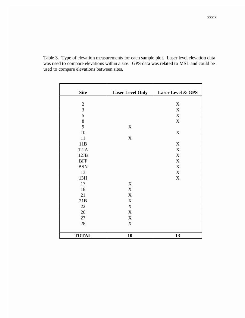
12. Length (km) of upland and transition soils along valley perimetersin each geographic region...................................................................................42
13. Length (km) of upland and transition soils along interfluveperimeters in each geographic region..................................................................42
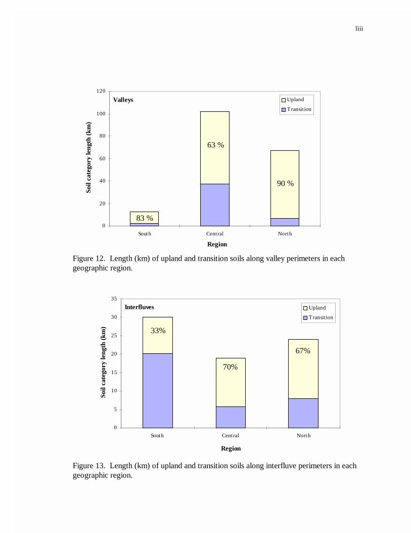
14. Length (km) of upland and transition soils along the perimeter of islands ............43
15. Length (km) of upland and transition soils along the perimeter of necks. ............43
16. Method used to portray field data as two plots per zone I the high marshand transition zones............................................................................................46

vi
17. Boxplots showing physical components of vegetation structure along a gradient from low marsh to forest...................................................................49
18. Boxplots showing dead vegetation components along a gradient fromlow marsh to forest.............................................................................................60
19. Boxplots showing depth of the organic rich horizon (cm) in each sample plot.....64
20. Boxplots showing the organic matter (%) of the soils (A) 0-10 cm and(B) subsurface (first 10 cm of the next deeper horizon), for eachvegetation zone..................................................................................................65
21. Boxplots showing salinity (ppt) of the soil (A) 0-10 cm and (B) subsurface(first 10 cm of the next deeper horizon), for each vegetation zone.......................66
22. Scatter plots showing the relationship between F1’s actual elevation and(A) the elevation difference between F1 and the average high marshelevation, or L2 where the high marsh zone was absent, and (B) theslope between L2 and F1....................................................................................76
23. The relationship between predicted and actual elevations of F1...........................77
24. Boxplots showing (A) actual elevation (m) above MSL and (B) actual and estimated elevation (m) above MSL, along a gradient from low marsh to forest..78
25. Ordination plot of forest sites using principal components analysis......................86
26. Variables (A) elevation above MSL, (B) slope between F1 and L2, (C)elevation of forest above adjacent seaward zone, and (D) soil type, used toclassify forest sites into three resistance groups: low (L), intermediate (I),and high (H).......................................................................................................87
27. Ordination plots of high marsh sites using principal components analysis.............90
28. Variables (A) elevation of high marsh above low marsh, (B) slope of highmarsh, (C) depth of organic rich zone from soil surface, (D) percent organicmatter (0-10 cm), and (E) elevation of high marsh above MSL, used toclassify high marsh sites into three resistance groups: low (L), intermediate (I), and high (H)................................................................................................91
29. Boxplots showing distance from the nearest tidal source for the (A) forest,(B) transition, and (C) high marsh grouped by resistance groups: low (L),intermediate (I), and high (H).............................................................................94

vii
30. Boxplots showing physical vegetation structure components for thethree forest resistance groups: low (L), intermediate (I), and high (H).................95
31. Boxplots showing dead vegetation components for forest resistance groups:low (L), intermediate (I), and high (H)................................................................99
32. Boxplots showing soil characteristics (A) salinity (0-10 cm), (B) depth oforganic rich soil beneath ground surface, (C) percent organic matter(0-10 cm) for forest resistance groups: low (L), intermediate (I), and high (H)...................................................................................................................100
33. Physical characteristics of transition sites grouped by their forestresistance groups: low (L), intermediate (I), and high (H).................................101
34. Boxplots showing vegetation structure components for transition sitesgrouped their forest resistance groups: low (L), intermediate (I), and high (H)...................................................................................................................103
35. Dead vegetation components for transition sites grouped by their forestresistance groups: low (L), intermediate (I), and high (H).................................107
36. Boxplots showing soil characteristics: soil salinity (0-10 cm), depth oforganic rich horizon from ground surface, and percent organic matter(0-10 cm) of transition sites grouped by their forest resistance groups:low (L), intermediate (I), and high (H)..............................................................108
37. Boxplots showing physical characteristics, not used in the classification, ofmarsh sites grouped by resistance: low (L), intermediate (I), and high (H).........109
38. Boxplots showing physical vegetation structure components for high marshresistance groups: low (L), intermediate (I), and high (H).................................111
39. Boxplots showing dead vegetation components for high marsh resistancegroups: low (L), intermediate (I), and high (H).................................................113
40. Map and field indicators for subgroups (A, B, C, D) of forest resistancegroups (low, intermediate, high).......................................................................117
41. Number and percent of map sites within each forest resistance subgroup..........120
42. Number of sites within each forest resistance group by geographic region.........120

viii
43. Pie charts showing percent of map sites in each forest resistance subgroupby geographic region........................................................................................122
44. Cross section of terrace plain through the three geographic regions...................124
45. Summary of changes that occur with each state change in response torising sea level..................................................................................................127
46. Examples of each forest resistance subgroup illustrated on soil survey maps and field cross sections............................................................................143

LIST OF TABLES
1. Soil categories, series, symbols, drainage classes, and great groups for soilspresent along map transects................................................................................17
2. Vegetation zones occurring along the eastern mainland fringe of the VirginiaCoast Reserve.....................................................................................................23
3. Type of elevation measurements for each sample plot.........................................28
4. Variables and scores used for forest state resistance classification.......................31
5. Variables and scores used for classification for high marsh state resistance..........33
6. Area (hectares) of soil categories and elevation intervals for the threegeographic regions..............................................................................................39
7. Length of coastline (boundary between forest and marsh) and percentof each forest soil category (transition = hydric, upland = nonhydric) alongthe coastline........................................................................................................44
8. Number of sample plots in each vegetation zone by site......................................48
9. Plant species present in the four vegetation zones...............................................52
10. Relative percent ground cover (0-1 m) of species or other cover type in eachvegetation zone..................................................................................................54
11. Importance values (IV) for woody species in the four vegetation zonesfor all field sites..................................................................................................56
12. Low marsh soil profile characteristics.................................................................62
13. High marsh soil profile characteristics.................................................................67
14. Transition soil profile characteristics...................................................................70
15. Forest soil profile characteristics.........................................................................73
16. Elevation averages for plots and zones, and elevation differences withinplots and between zones.....................................................................................80
x
17. Vegetation characteristics (A) physical structure, and (B) relative %ground cover (0-1 m) and species IVs for groundwater seeps......................... ...81
18. Elevation, zone width, and soil characteristics for ground water seeps.................83
19. Forest scores and ranks by resistance group: low (L), intermediate (I), andhigh (H)..............................................................................................................85
20. High marsh scores and ranks by resistance group: low (L),intermediate (I), and high (H).............................................................................89
21. Relative percent ground cover (0-1 m) and woody species IVs for forestresistance groups: low (L), intermediate (I), and high (H)...................................97
22. Relative percent ground cover (0-1 m) and woody species IVs fortransition sites grouped by their forest resistance group: low (L),intermediate (I), and high (H)............................................................................105
23. Relative percent ground cover (0-1 m) and woody species IVs forhigh marsh sites grouped by their resistance group: low (L),intermediate (I), and high (H)............................................................................112
24. Field sites listed with their respective zones and zone widths.............................114
25. Map characteristics for each field site grouped by their subdivided forestresistance group................................................................................................116

xi
1. INTRODUCTION
Sea level has fluctuated throughout the course of geologic history, and currently it
is rising. The rate at which sea level rises or falls has varied through time and is specific
for a given location (Braatz and Aubrey 1987, Pirazzolia 1989). For this study, the
context of a rising sea is used because it is the prevailing condition. The cause of sea level
rise is a topic of current interest with several hypothesis under investigation. Some of
these include glacio-eustatic changes, tectonic movements, changes in oceanic currents,
and cyclic orbital forcing of oceanic and climatic changes (Milankovitch cycles) (Gornitz
and Lebedeff 1987, Dott 1992). In addition, a recent effort has been undertaken to
discern the effects that anthropogenic activities have on climate change and sea level rise.
Some scientists believe that increasing atmospheric concentrations of carbon dioxide and
other gases released by human activities are expected to warm the earth a few degrees
Celsius in the next century by a mechanism known as the greenhouse effect (Titus 1987).
They predict this warming will accelerate the rate of sea level rise.
Many studies have been conducted to determine the extent of global warming and
its effects on sea level rise. The Intergovernmental Panel on Climate Change (IPCC 1995)
reported that over the past century the mean global surface air temperature had increased
between 0.3 and 0.6o C. During this same 100 year period, sea level has risen between 10
and 25 cm. The researchers project this trend will likely continue in the future.
With the use of models, the IPCC developed a series of scenarios for prediction of
global temperature and sea level changes by the year 2100. Under the extreme low
scenario, they predicted a 1o C increase in temperature and a 1 mm/year rise in sea level

xii
for a total of a 15 cm rise in sea level. Under the medium scenario, the IPCC predicted a
2o C rise in air temperature by 2100, and a probable 50 cm rise in sea level. Under the
extreme high scenario they predicted 3.5o C increase in air temperature, and a rise in sea
level equivalent to 9 - 10 mm/year for a total rise of 95 cm by the year 2100.
With the use of different models, other researchers have conducted similar studies
to discern the extent of future sea level rise. Meier (1990) and Church et al. (1991)
predict a 30 and 35 cm rise respectively, by the year 2050. Wigley and Raper (1992,
1993) estimate that sea level rise will be 4-5 times faster over the next century and foresee
a 46 - 48 cm rise by 2100. Titus and Narrayanan (1995) predict a 34 cm rise in sea level
by the year 2100. Despite the differences in the models employed, all of these recent best
estimate predictions for future sea level rise fall within a range of 3 - 6 cm/decade (IPCC
1995).
A minor rise in sea level could cause a reduction in the world’s coastal wetlands
because most of them are within a few meters of current sea level (Titus 1991). A rise in
sea level can disrupt wetlands in three major ways: salt water intrusion, flooding, and
erosion. Depending on a wetland’s landscape position, these forces may act to convert a
wetland to an open body of water or tidal mud flat or change the vegetational composition
of a wetland. The degree to which coastal wetlands will be affected by rising sea level
depends on (1) the ability of the wetland to accrete either by mineral sediment deposition
or autogenic peat accumulation, (2) the subsidence rate of the wetland, and (3) the
distance available for marsh transgression over higher land.
xiii
The ability of a coastal wetland to accrete depends on the amount of mineral
sediment input it receives and its ability to accumulate peat. Mineral sediment availability
to a marsh depends on its tidal range, and size and erodability of its watershed. The
coastal marshes of North Carolina’s Pamlico and Albemarle Sounds are examples of areas
with low tidal ranges (Moorehead and Brinson 1995, Young 1995). In contrast, mineral
sediment deficits along the southern Delmarva Peninsula may be due to small watershed
sizes (Oertel et al. 1992). Marshes deficient in both mineral and organic sediment have
lower rates of accretion and are more prone to submergence. Many studies have been
conducted to determine accretion rates and results indicate these rates are highly variable
both temporally and spatially (Stevenson et al. 1986, Hackney and Cleary 1987, Cahoon
and Lynch 1997). In some marshes peat accumulation and sediment deposition are
sufficient to keep pace with the rising sea. For these marshes, net wetland acreage is
either preserved or increased (Orson et al. 1985). However, in many marshes the rate of
subsidence may negate any vertical growth due to accretion (Cahoon and Lynch 1997).
Deep subsidence may occur as a result of human induced activities such as oil and
gas drilling, the dewatering of aquifers (Poland and Davis 1969), and shallow subsidence
can occur from oxidation of peat due to increased drainage. Also, as sediment loading
occurs, shallow compaction of the land causes a decrease in marsh elevation (Kaye and
Barghoorn 1964, Stevenson et al. 1986). If accretion rates are unable to keep pace with
subsidence rates or sea level rise, then the relative rate of marsh flooding increases
(Nyman et al. 1993).

xiv
In response to rising sea level, coastal salt marshes naturally migrate over land
(Fletcher et al. 1990, Oertel et al. 1992, Gardner et al 1992, Young 1995). During this
process, tidal flat is converted to open water, intertidal mineral low marsh is converted to
tidal flat or open water, organic high marsh is converted to mineral low marsh, and
forested wetland or upland is converted to organic high marsh (Brinson et al. 1995).
These conversions are termed state changes in contrast to successional changes because
they are reliant upon external controls for their initiation (Brinson et al. 1995, Hayden et
al. 1995). One would presume these state changes would conserve the area of wetland
and a net decrease in forest would result. However, if the slope between the marsh and
the upland is great or if impeding structures such as roads, dikes, or buildings have been
constructed, then the migration of the marsh ceases (Kayan and Kraft 1979). As sea level
continues to rise and open water moves landward, wetlands have no new surface area
available, and consequently they diminish in size (Oertel and Woo 1994).
Evidence of the Holocene transgression has been documented for many areas.
Some of these areas include Louisiana (Salinas et al. 1986), South Carolina (Gardner et al.
1992), North Carolina (Young 1995), Virginia (Hayden et al. 1991, Kastler and Wiberg
1995), New York (Clark 1986), and New Brunswick, Canada (Robichaud and Begin
1997). One specific example of transgression is demonstrated in a study conducted by
Downs et al. (1994) on Bloodsworth Island, an island located in the Maryland portion of
the Chesapeake Bay. The authors report a decline of 579 ha or 26 % of total land area for
Bloodsworth Island between 1849 and 1992. Initially, the island’s response to sea level
rise was upland conversion to wetland; 79 % of island’s 1849 upland area was lost by
xv
1973, and hence there was no significant net change in wetlands. However, due to lack of
available upland surface and rising rates in sea level, wetland loss is presently exceeding
wetland gains.
For the purpose of coastal land management, it would be useful to develop an
accurate methodology for predicting the future of a given landscape in response to rising
sea level. To ensure this, in-depth field measurements would need to be taken at a very
small scale (i.e. elevation measurements to the centimeter). Under most circumstances,
this approach is unrealistic for large areas because of time and money constraints. A more
practical approach would be to rely on maps to determine areas more susceptible to sea
level rise. By employing a combination of soil survey maps, National Wetland Inventory
maps, USGS topographic maps and aerial photographs in conjunction with field
measurements, it may be possible to decipher many landscape features important in
determining the fate of coastal land in response to rising sea level.
Several models that employ the use of map information have been developed to
determine the extent of land class changes in response to sea level rise. Lee et al. (1991)
developed a simulation model that predicted 40 % of the wetlands along the coast of
northeastern Florida would be lost under a 1 m rise in sea level. The majority of that
wetland loss was comprised of low marsh.
Kana et al. (1987a,b) developed a simple geometric model which they used to
predict the reduction in coastal marshes under different scenarios of sea level rise by the
year 2075 for two Atlantic coastal cities. For Charleston, SC under the low scenario of an
87 cm rise in sea level, there would be a net loss of about 59 % of the marsh and a 100 %

xvi
increase in tidal flats. The high scenario (159 cm) would result in an 80 % net reduction
of wetlands. For Tuckerton, NJ under the low scenario of sea level rise, there would not
be a major loss of total marsh acreage, although 90 % of the high marsh would be
converted to low marsh. In the higher sea level rise scenario, 86 % of the marsh would be
lost.
Another model developed by Park et al. (1991) is a spatial cell-based simulation
model named SLAMM (Sea Level Affecting Marshes Model). This model was used on a
much larger scale to predict the effects of a 1 m rise in sea level within the next century.
They determined there would be a 26 to 82 % reduction in coastal wetlands within the
conterminous United States.
Equipping ourselves with the knowledge of locations most likely to be intercepted
by sea level rise could prove to be economically, socially, and environmentally
advantageous. For the purpose of maintaining wetland ecosystems, it would be prudent to
preserve areas most susceptible to sea level rise for marsh transgression. Furthermore,
identifying these areas would steer potential developers and other property buyers from
these high risk areas and avoid future losses.
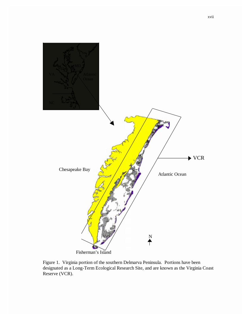
The southern portion of the Delmarva Peninsula, which is bound on the east by the
Atlantic Ocean and on the west by the Chesapeake Bay (Figure 1), is an area experiencing
xvii
Figure 1. Virginia portion of the southern Delmarva Peninsula. Portions have beendesignated as a Long-Term Ecological Research Site, and are known as the Virginia CoastReserve (VCR).
NC
VA
MD
AtlanticOcean
Atlantic OceanChesapeake Bay
N
Fisherman’s Island
VCR

xviii
xix
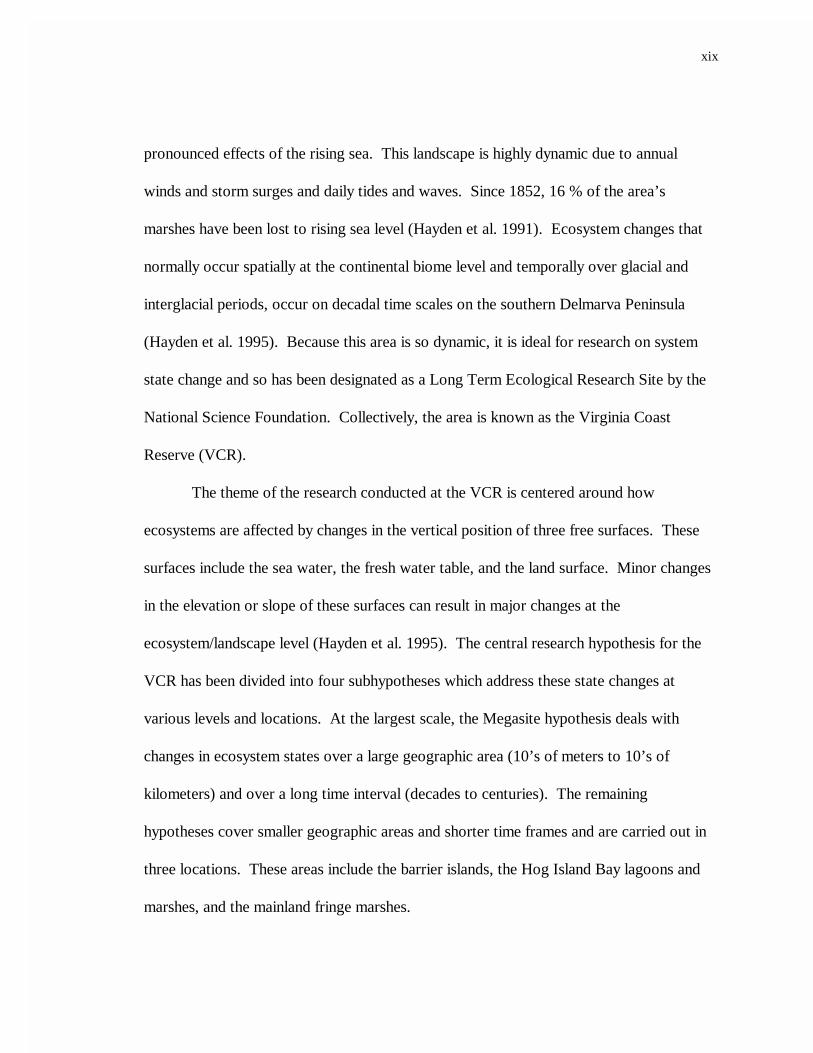
pronounced effects of the rising sea. This landscape is highly dynamic due to annual
winds and storm surges and daily tides and waves. Since 1852, 16 % of the area’s
marshes have been lost to rising sea level (Hayden et al. 1991). Ecosystem changes that
normally occur spatially at the continental biome level and temporally over glacial and
interglacial periods, occur on decadal time scales on the southern Delmarva Peninsula
(Hayden et al. 1995). Because this area is so dynamic, it is ideal for research on system
state change and so has been designated as a Long Term Ecological Research Site by the
National Science Foundation. Collectively, the area is known as the Virginia Coast
Reserve (VCR).
The theme of the research conducted at the VCR is centered around how
ecosystems are affected by changes in the vertical position of three free surfaces. These
surfaces include the sea water, the fresh water table, and the land surface. Minor changes
in the elevation or slope of these surfaces can result in major changes at the
ecosystem/landscape level (Hayden et al. 1995). The central research hypothesis for the
VCR has been divided into four subhypotheses which address these state changes at
various levels and locations. At the largest scale, the Megasite hypothesis deals with
changes in ecosystem states over a large geographic area (10’s of meters to 10’s of
kilometers) and over a long time interval (decades to centuries). The remaining
hypotheses cover smaller geographic areas and shorter time frames and are carried out in
three locations. These areas include the barrier islands, the Hog Island Bay lagoons and
marshes, and the mainland fringe marshes.
xx
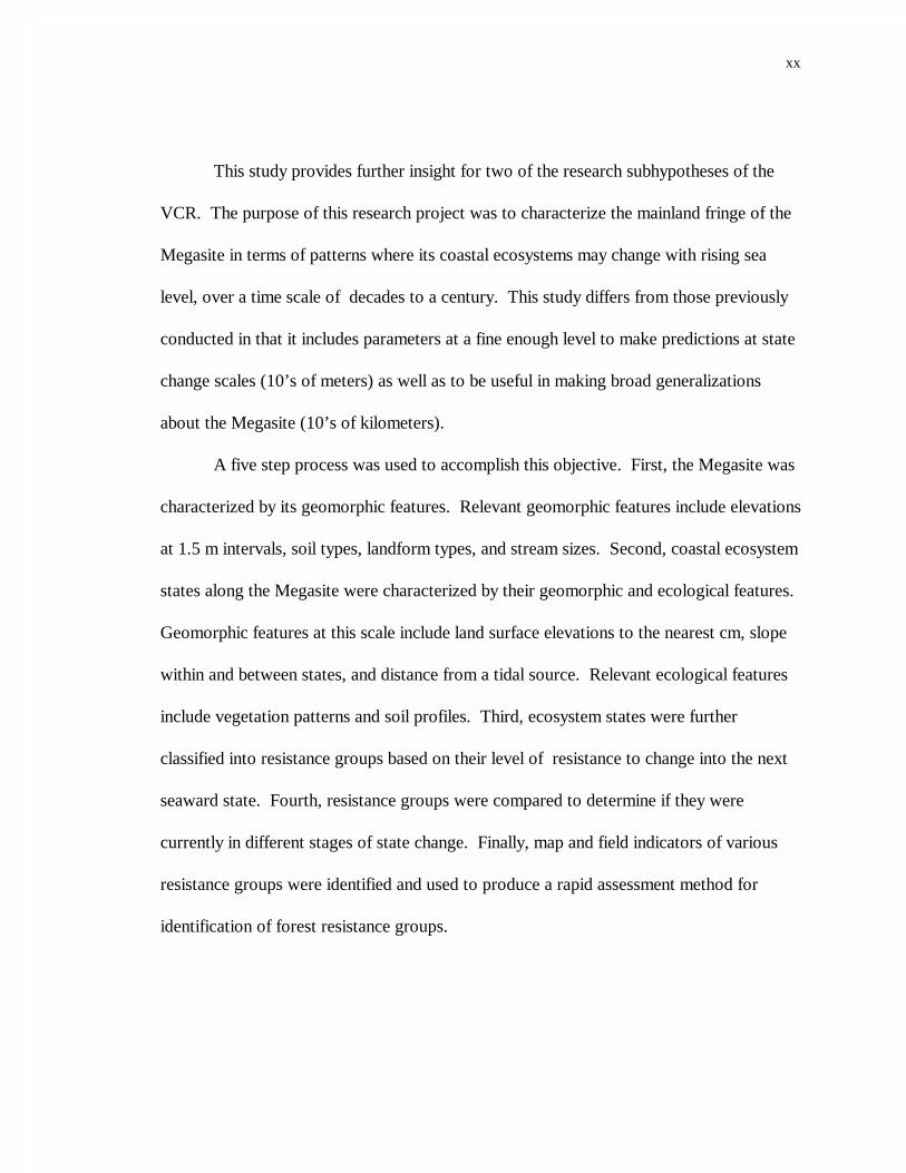
This study provides further insight for two of the research subhypotheses of the
VCR. The purpose of this research project was to characterize the mainland fringe of the
Megasite in terms of patterns where its coastal ecosystems may change with rising sea
level, over a time scale of decades to a century. This study differs from those previously
conducted in that it includes parameters at a fine enough level to make predictions at state
change scales (10’s of meters) as well as to be useful in making broad generalizations
about the Megasite (10’s of kilometers).
A five step process was used to accomplish this objective. First, the Megasite was
characterized by its geomorphic features. Relevant geomorphic features include elevations
at 1.5 m intervals, soil types, landform types, and stream sizes. Second, coastal ecosystem
states along the Megasite were characterized by their geomorphic and ecological features.
Geomorphic features at this scale include land surface elevations to the nearest cm, slope
within and between states, and distance from a tidal source. Relevant ecological features
include vegetation patterns and soil profiles. Third, ecosystem states were further
classified into resistance groups based on their level of resistance to change into the next
seaward state. Fourth, resistance groups were compared to determine if they were
currently in different stages of state change. Finally, map and field indicators of various
resistance groups were identified and used to produce a rapid assessment method for
identification of forest resistance groups.

xxi
2. SITE DESCRIPTION
The study site is 99 km in length and extends from Cape Charles, VA north to
Wallops Island, VA (Figure 1). In general, the southern portion of the Delmarva
peninsula is comprised of a central upland bordered on the east and west by a series of
terrace plains and lowlands (Mixon 1985) (Figure 2). The Metomkin, Mappsburg, and
Kiptopeake scarps delineate the boundary between the central upland and the eastern
terrace plains. These terrace plain surfaces are comprised of agricultural fields, upland and
wetland forests, and salt marshes depending on the surface elevation, soil type, and
proximity to a brackish water source. The central upland ranges from 10-19 m (35-60 ft)
in elevation and the eastern terrace plains range from sea level to 8 m (26 ft) in elevation.
To the east of the terrace plains lies a complex of salt marshes, tidal flats, lagoons, and
barrier islands.
The study site ranges from 0.4 to 4.5 km in width, and extends from the 7.6 m (25
ft) contour line on the west, through the eastern terrace plains, and ends at the estuarine
boundary on the east. Within the study area, there are three major terrace plains which
include the Metomkin plain, Kiptopeke plain, and the Bell Neck Sand-Ridge complex
(Mixon 1985). These plains extend for approximately 99 km from north to south with
some overlap between them. The Metomkin plain lies the farthest north. It ranges in
elevation from 7-8 m (23-26 ft) at the toe of the Metomkin scarp to 5 m (16 ft) or less at
the western edge of the coastal lagoon and is approximately 41 km long. The Kiptopeke
plain extends from Cape Charles north-northeast for about 16 km to where it is intersected
by the Mappsburg scarp. This plain ranges in elevation from 8 m (25 ft) at the toe of the

xxii
Figure 2. Geomorphic features of the southern Delmarva Peninsula and the threegeographic regions defined for this study. The division of the three geographic regionscorresponds to the presence of a series of relict regressive ridges in the central region.
0 10
ATLANTIC OCEAN
Hog Island
Wallops IslandCHESAPEAKE BAY
SOUTHREGION
NORTHREGION
CENTRALREGION
Metomkin plain
Bell Neck Sand-Ridge complex
Kiptopeake plain
Marsh
Barrier Island
N
xxiii
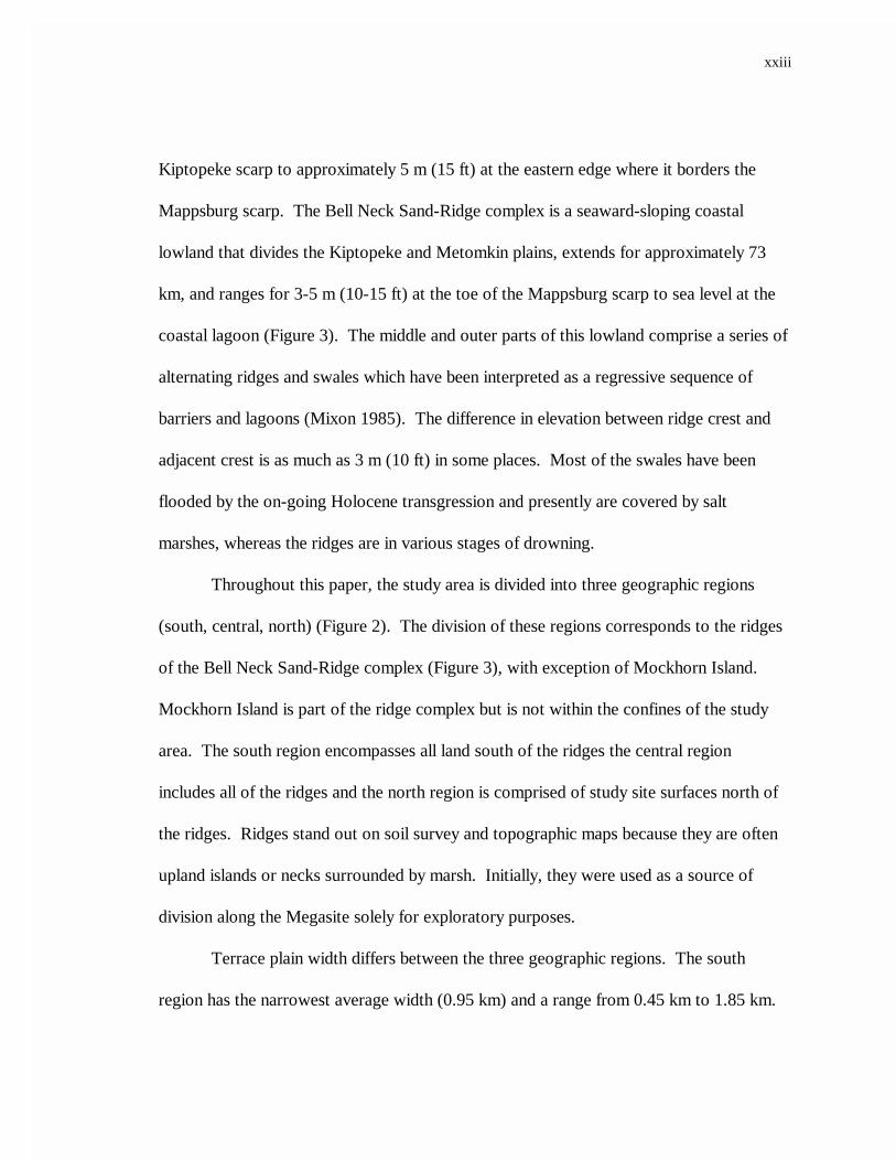
Kiptopeke scarp to approximately 5 m (15 ft) at the eastern edge where it borders the
Mappsburg scarp. The Bell Neck Sand-Ridge complex is a seaward-sloping coastal
lowland that divides the Kiptopeke and Metomkin plains, extends for approximately 73
km, and ranges for 3-5 m (10-15 ft) at the toe of the Mappsburg scarp to sea level at the
coastal lagoon (Figure 3). The middle and outer parts of this lowland comprise a series of
alternating ridges and swales which have been interpreted as a regressive sequence of
barriers and lagoons (Mixon 1985). The difference in elevation between ridge crest and
adjacent crest is as much as 3 m (10 ft) in some places. Most of the swales have been
flooded by the on-going Holocene transgression and presently are covered by salt
marshes, whereas the ridges are in various stages of drowning.
Throughout this paper, the study area is divided into three geographic regions
(south, central, north) (Figure 2). The division of these regions corresponds to the ridges
of the Bell Neck Sand-Ridge complex (Figure 3), with exception of Mockhorn Island.
Mockhorn Island is part of the ridge complex but is not within the confines of the study
area. The south region encompasses all land south of the ridges the central region
includes all of the ridges and the north region is comprised of study site surfaces north of
the ridges. Ridges stand out on soil survey and topographic maps because they are often
upland islands or necks surrounded by marsh. Initially, they were used as a source of
division along the Megasite solely for exploratory purposes.
Terrace plain width differs between the three geographic regions. The south
region has the narrowest average width (0.95 km) and a range from 0.45 km to 1.85 km.

xxiv
Figure 3. Bell Neck Sand-Ridge complex of the central region and adjacent barrierislands. Figure is modified from Figure 23 in Mixon (1985).
Marsh
Bell Neck Lowland
Bell Neck Sand-Ridge
Barrier Island
Kilometers
0 2 4 6
Mappsburg Scarp
ParramoreIsland
Hog Island Bay
ATLANTICOCEAN
N
xxv
The central region has the widest terrace plain on average (3.2 km) and ranges in width
from 0.74 km to 4.5 km. The north region has an average terrace plain width of 1.9 km
and a range from 0.4 km to 3.3 km. The width of the marsh-tidal flat-lagoon complex
varies along the length of the peninsula. This complex is widest within the central region
and ranges between 4.5 - 13 km. The complex is narrowest in the north region where it
ranges in width between 7.5 and 13 km. The width of the south region’s marsh-tidal flat-
lagoon complex ranges from 7.5 to 13 km.

xxvi
3. METHODS
3.1 Megasite Characterization
Maps were used to characterize large scale geomorphic features of the Megasite.
Transects were delimited, within the three geographic regions, on soil survey maps,
National Wetland Inventory (NWI) maps, and United States Geological Survey (USGS)
topographic maps. Map transects were oriented perpendicular to the coastline and scarps
(Kiptopeake, Mappsburg, or Metomkin Scarp, whichever was farthest west) and extended
from the 7.6 m (25 ft) contour line east to the estuarine boundary. For this study, the
estuarine boundary demarks the location where the eastern most upland or marsh
boundary of the study area meets open water. Map transects were placed every 3300 m
along the length (north-south) of the study area (99 km) for a total of 30 transects (Figure
4).
Ten different soil series occurred along the map transects (USDA 1989 and 1994).
These were grouped into three categories: marsh, transition, and upland soils. The marsh
category includes the two hydric soil series present in marshes; transition soils include all
hydric soils that do not exist in marshes; and the upland category includes all nonhydric
soils (Table 1). For purposes of characterization, transect elevations above mean sea level
(MSL) were divided into three intervals (0-1.5 m, 1.5-3.0 m, 3.0-7.6 m). Along each map
transect, the proportion of the total transect width representing each soil series and
elevation interval was measured. Distances or proportions measured along transects (east
to west orientation) will be referred to as widths rather than lengths to avoid confusion
with region or study site length (north to south orientation). In addition, the area (ha) of

xxvii
Figure 4. Geomorphic map of Virginia Coast Reserve showing approximate location ofmap transects. Map transects are labeled with their corresponding number.
0 10
ATLANTIC OCEAN
Hog Island
Wallops IslandCHESAPEAKE BAY
SOUTHREGION
NORTHREGION
CENTRALREGION
1
2
3
4
5
6
7
8
9
1011
12
13
1415
1617
18
19
20
21
22 23
24 25
26
27
2829
30
Metomkin plainBell Neck Sand-Ridge complex
Kiptopeke plain
Marsh
Barrier Island
N

xxviii
Table 1. Soil categories, series, symbols, drainage classes, and great groups for soilspresent along map transects (USDA 1989, 1994). The three different soil symbolsassociated with the Bojac soil series represent different texture types (BoA = fine sandyloam, BkA = sandy loam, BhB = loamy sand).
Soil Category Soil Series Soil SymbolDrainageClass* Great Group
Marsh ChincoteagueMagotha
ChA**MaA**
VPDPD
Typic SulfaquentsTypic Natraqualfs
Transition NimmoArapahoeDragstonPolawanaCamocca
NmA**ArA, AhA**DrA**PoA**CaA**
PDVPDSPDVPDPD
Typic OchraquultsTypic HumaqueptsAeric OchraquultsCumulic HumaqueptsTypic Psammaquents
Upland MundenBojacMolenaUdorthents
MuABoA, BkA, BhBMoDUpD
MWDWDSEDSPD - WD
Aquic HapludultsTypic HapludultsPsammenticHapludultsUdorthents
* VPD = very poorly drained, PD = poorly drained, SPD = somewhat poorly drained,MWD = moderately well drained, WD = well drained, SED = somewhat excessivelydrained** = hydric soil

xxix
soil types and elevation intervals were calculated for each region. Area was determined by
multiplying the length of each region by the average width of the transects it encompassed.
For each region, data was collected on the number of streams it contained and
each stream’s order and length. Stream attributes were only measured for the portion of
the creek within the mainland, rather than following it until it entered the lagoon or ocean.
Stream order was determined using Strahler’s classification (Strahler 1957). Stream
length is the sum of all branches entering into a creek.
I identified 4 major landform types (valley, interfluve, neck, island) (Figure 5)
within the study area that were modified from a marsh classification described by Oertel
and Woo (1994). I characterized the perimeter of each landform by its length and soil
abundance by series. Perimeter length was traced along the boundary between the marsh
and forest soils (upland or transition) bordering each landform perimeter (see Figure 5).
Valleys are landforms encompassing creeks currently being drowned by the
Holocene transgression and as a result contain marsh soils. Because the main focus of this
study concerns changes occurring on land surfaces rather than within the marsh, I use the
term valley landform to describe the land surface fringing the drowned creek valley. Not
all creeks were considered valleys; only land fringing creeks that contained marsh soils
were classified as valley landform. Interfluves are the portion of the mainland between
valley landforms. Valley and interfluve landforms occur at several different scales; so for
clarity, those defined in this study were identified at scales detectable on soil survey maps
(1:15,800).

xxx
Land
Marsh
Creek
VALLEY - Land surroundingmarsh contained within a valley.
INTERFLUVE -portion of land positionedbetween valleys.
NECK - land surrounded bymarsh on three sides with aconnection to the mainland.Necks are remnant Bell Neckridges.
ISLAND - landcompletely severed from themainland and surrounded bymarsh on all sides. Islandsare remnant Bell Neck ridges.
Figure 5. Landforms along the mainland fringe of the Virginia Coast Reserve. Fourtypes of landforms were identified: valley, interfluve, neck, and island. The perimeter ofeach landform type is outlined differently so landforms can be distinguished. Ahypothetical field transect is shown crossing two landforms with different sample sitesrepresented by boxes. Landforms were identified on soil survey maps which are at ascale of 1:15,800.
Valley perimeter
Neck perimeter
Interfluve perimeter
Island perimeter

xxxi
Necks and islands are remnant Bell Neck ridges (Figure 3) that are in different
stages of drowning. Ridges still attached to the mainland, but are predominately
surrounded by marsh, are classified as necks. Necks are surrounded by marsh on three
sides. Portions of necks still connected to the mainland were classified as interfluve.
Necks often contribute a portion of their area to valley landforms. For locations where
this occurs, neck surface is classified as neck rather than valley. Segments of land
surrounded by marsh on three sides in the larger northern valley marshes (from
Nicciwampus Creek north) were not classified as necks because they do not correspond to
relict Bell Neck ridges. These are distinguishable from necks corresponding to Bell Neck
ridges because they have a coast-normal orientation as opposed to the coast-parallel
orientation of the Bell Neck ridges. Islands have been completely severed from the
mainland and are surrounded by marsh on all sides.
Aerial photos from 1939 and 1941 were compared with photos from 1990 to
determine if significant changes in the Megasite’s zonation had occurred over the past 50
years in the vicinity of the transects. The earlier photos were at a scale of 1:20,000 and
the more recent photos were at a scale of 1:660. This procedure’s resolution was limited
by the large scale of the earlier photos.
3.2 Ecosystem State Characterization
Field transects, a subset of the map transects, were used for ecosystem state
characterization. The selection of transects for field sampling was based on accessibility
and the degree of land alteration. Locations corresponding to map transects that were

xxxii
inaccessible or had been considerably altered by silviculture, construction, or
impoundment activities were not used as field transects, or a location adjacent to them
was chosen. For these reasons, several of the field transects differ from their
corresponding map transect location. For some field transects, several positions along the
transect were used to characterize ecosystem states; therefore, each location sampled
along a field transect is referred to as site. A total of 20 sites from 16 field transects were
sampled. In addition, three sites (BFF, BSN, 21B) not corresponding to map transects
were sampled, for a total of 23 field sites (Figure 6). The additional sites were used
because they were easily accessible and increased the field sample size. Several sites were
chosen along a single field transect where various landforms were present. I ensured that
all of the soil drainage classes and landforms were encompassed in the sites used for field
sampling.
Sites were subdivided into 4 vegetation zones (forest, forest-marsh transition, high
marsh, low marsh) which correspond to ecosystem states (Table 2). Each state has a
unique suite of characteristics associated with it other than vegetational differences
(Brinson et al. 1995). However, vegetation was used solely to delineate states in the field
because plants were reliable indicators and rapidly identifiable. Therefore, I characterized
each vegetation zone by its soil, vegetation, and elevational features. The sampling unit
used for this characterization is termed a plot (Figure 7). Plots consisted of a 12 m
diameter circle with the center point located on the field transect. I decreased the width of
the plot diameter for vegetation zones with widths between 9 and 12 m. Two semicircles

xxxiii
Figure 6. Geomorphic map of Virginia Coast Reserve showing approximate location ofsites sampled in the field. Field transects with two sites are marked with an asterisk * anda field transect with three sites is marked with two asterisks **. Three sites (BFF, BSN,21B) do not correspond to a map transect and are noted with an arrow.
0 10
ATLANTIC OCEAN
Hog Island
Wallops IslandCHESAPEAKE BAY
SOUTHREGION
NORTHREGION
CENTRALREGION
2
3
5
8
9
10
11*
12** 13*
17
18
21
22
26
27
28
SitesBFF & BSN
Site21B
N
Metomkin plain
Bell Neck Sand-Ridge complex
Kiptopeake plain
Marsh
Barrier Island

xxxiv
Table 2. Vegetation zones occurring along the eastern mainland fringe of the VirginiaCoast Reserve.
Vegetation Zone Description
Forest Zone dominated by trees and lacking marsh grasses.
Forest - Marsh Transition Zone dominated by shrubs or small trees with thepresence of marsh grasses.
High Marsh Zone dominated by the marsh grasses Spartina patens orDistichlis spicata, or the rush Juncus roemarianus.Shrubs may be present but fall below 50% cover.
Low Marsh Zone dominated by the marsh grass, Spartinaalterniflora.

xxxv
Sample PlotThe typical diameter of the sample plotwas 12 m. Percent cover was describedfor three evenly spaced 1 m2 quadratswithin each sample plot.
Figure 7. Field transects, sites, and sample plots. Sampling locations along field transectsare referred to as sites. One to three sites were sampled along each field transect. Siteswere divided into vegetation zones: forest, transition, high marsh, and low marsh. Withineach vegetation zone, sample plots were used to collect data on vegetation, soil, andelevation characteristics. Three forest and two low marsh sample plots were placed in thesame location at all sites for consistency. The number of plots sampled in the transitionand high marsh increased with increasing zone width, with a maximum of four sampleplots for a zone width of 202 m. These plots were evenly spaced along the transect withinthe zone. Each sample plot was numbered consecutively starting at the seaward side ofthe zone. Figure is not to scale.
FOREST TRANSITION HIGH MARSH LOW MARSH
L1F2F3 L2T2F1 T1 H2 H1
61830 6 180 0
Distance of plots from zone edge (m) Spacing varies with zone width
Field Transect with two sites
Site: sampling position along a field transect. Sites weredivided into four vegetation zones. Each vegetation zone hasbetween one and four sample plots.

xxxvi
were used as the sampling unit for zones with widths <9 m. The number of plots sampled
in a given zone depended on the type of vegetation zone, zone width, and vegetation
heterogeneity. For purposes of cross-site comparison, forest and low marsh sampling
plots were consistently placed. Generally three plots were sampled in the forest and two
in the low marsh with the center points located at 6, 18, and 30 m from the zone edge for
the forest and 6 and 18 m from the zone edge for the low marsh. Fewer sample plots were
used where zone width did not accommodate this configuration. The number of sampling
plots for the high marsh and transition zones varied depending on zone width and were
spaced evenly apart. Typically high marsh and transition zones had two sample plots but a
few had as many as four or as few as one. Both forest and marsh zones were
characterized similarly so that they were easily comparable during data analysis. Where
applicable, six measurements were made for each sampling plot. First, the basal area
(m2/ha cross sectional area at 1.5 m above ground) for all live trees, by species, and dead
trees >1m in height and >10 cm in diameter at 1 m in height were measured using calipers.
Second, counts of live and dead trees and shrubs >1m in height, by species, were made.
Third, using a 1 m2 quadrat, percent cover was determined for two height intervals (0-1 m
and 1-3 m). Percent cover estimates included the following classes: (1) vegetation by
species, (2) dead trees (>1m tall), (3) dead shrubs, (4) natural stumps (<1m tall), (5) litter,
(6) bare ground, (7) wrack, (8) potholes, (9) fiddler crab burrows, and (10) woody debris.
Also, the percent cover of the canopy above 3 m was determined using a cylindrical tube
for sighting. For all vertical positions, percent cover was estimated as the midpoint of one
of the following eight cover classes: 0% (0%), 0 - 5% (2.5%), 5 - 25% (15%), 25 - 50%
xxxvii
(37.5%), 50% (50%), 50 - 75% (67.5%), 75 - 95% (85%), 95 - 100% (97.5%), and 100%
(100%) (derived from Daubenmire 1968). Because cover classes were used rather than
discrete values, cover percentages can exceed 100 %. Three sets of quadrat samples were
taken within each circular plot. The quadrats were centered on the transect and were
evenly spaced within the plot (Figure 7). Fourth, counts were made of all vines at 1.5 m in
height. Fifth, the approximate age of the forest was determined by coring one of the older
looking trees at 1.5 m in height. Finally, because the vegetation zones are not detectable
on maps, their width was measured in the field.
Soil profile characteristics were evaluated at the midpoint of each vegetation zone.
Soils were excavated using a soil auger and were described to a variable depth depending
on the resistance of the soil, generally to a depth of at least 40 cm. Each soil horizon was
described in terms of soil matrix color, mottle matrix color, mottle abundance, and texture.
Soil colors were determined using the Munsell color chart and texture was determined by
feel analysis (Thien, 1979). In addition, the first 10 cm of the soil and the first 10 cm of
the next deeper horizon were brought back to the lab for determination of percent loss on
ignition and salinity. Finally, the depth of the organic-rich horizon, when present, was
measured at the midpoint of each sample plot.
Loss on ignition was determined for a sample of the soil surface (0-10 cm) and
subsequent horizon (first 10 cm), for all sites, as an estimate of percent organic matter.
First, the soil was homogenized by kneading it thoroughly in a ziplock bag. A portion of
the homogenized soil was oven dried at 100 C until dry. Next, the dry mass of the soil
was determined to the nearest 0.001g. The soil was then burned in a muffle furnace at

xxxviii
480 C for 3 h and then reweighed. The difference in mass was presumed to be the mass of
the organic matter. This weight is reported as the percent of total soil mass. Triplicates
for each soil sample were processed and their average is reported.
Soil salinity was determined for the soil surface and subsequent horizon, for all
sites. A portion of the homogenized soil, described in the above section, was allowed to
air dry for several days. A known mass of soil was mixed with a volume of distilled water
twice the mass of the soil. This mixture was then shaken mechanically for 1 h. Next, the
mixture was filtered through a glass fiber filter and then through a membrane filter with
0.80 µm pore size. For samples with clay, the mixture was filtered through a second
membrane filter with pore size 0.45 µm. A YSI model 30 salinity, conductivity, and
temperature meter was used to determine the salinity (ppt) of the filtrate. Of course, this
is one of many ways to measure soil salinity.
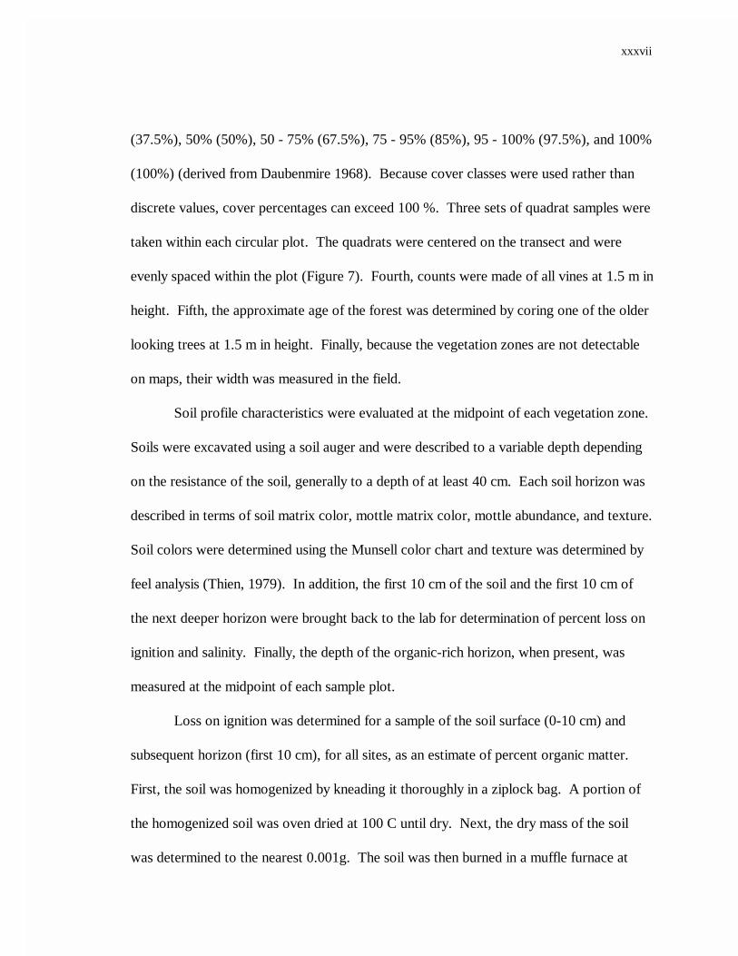
The elevation of each sample plot was determined, at its center point, using a laser
level. However, because there were rarely permanent benchmarks within the marshes,
these elevations were not tied into mean sea level (MSL) and hence are not directly
comparable among sites. A global positioning system (GPS) unit was used to determine
the elevation above MSL for a portion of the study sites (Table 3). The GPS receiver
used was a Trimble 4000 SE unit (L1 only) and the software used to process GPS data
points was GPSurvey 3.20a. The elevations generated from the GPS are tied into MSL,
according to the 1929 National Geodetic Survey, using a permanent bench mark (VCR1)
xxxix
Table 3. Type of elevation measurements for each sample plot. Laser level elevation datawas used to compare elevations within a site. GPS data was related to MSL and could beused to compare elevations between sites.
Site Laser Level Only Laser Level & GPS
2 X3 X5 X8 X9 X10 X11 X
11B X12JA X12JB XBFF XBSN X13 X
13H X17 X18 X21 X
21B X22 X26 X27 X28 X
TOTAL 10 13

xl
that has been established as a cignet global network tie. Detailed information concerning
the establishment of the VCR1 benchmark can be found at internet address:
www.vcrlter.virginia.edu/~crc7m/gps.html. Due to the high precision of the VCR1
benchmark, GPS elevations are accurate to the nearest centimeter and, therefore, can be
used to compare sites. Two variables (slope and elevation) that were correlated with the
forest elevation above MSL were used to develop a multiple regression equation. This
equation was utilized to estimate the elevations above MSL for sites that were not near
permanent bench marks.
3.3 Ecosystem State Classification
Forest and high marsh sites were each classified into three groups based on their
level of resistance to change into the next seaward state. The transition was not classified
because it is an intermediate stage between the forest and high marsh states. The low
marsh was not classified because only the landward 24 m was characterized and this was
not considered representative of the entire state. Variables used for the classification
determine the extent to which brackish water is able to reach a site, and how long it will
remain there. It is postulated that stressors introduced from stochastic storm events in
addition to the slow drowning of the land drive state change (Brinson et al. 1995, Young
1995). Therefore, several variables were used to classify sites into resistance groups
rather than zone elevation above MSL alone. These variables differ for the forest and high
marsh.

xli
Variables used to classify forest sites include elevation of forest above MSL,
elevation of forest above adjacent seaward zone, slope between forest and low marsh, and
forest soil drainage class. The two variables describing forest elevation determine the
extent to which brackish water can reach the forest. Slope and soil drainage class
determine the drainage potential of the forest, and subsequently the duration in which
brackish water will persist in forest soils.
Three types of procedures were used to classify forest sites. First, each of the four
variables were assigned a set of scores for all possible values (Table 4). Values were
based on a 15 cm rise in sea level. This estimate corresponds to the IPCC’s (1995) low
estimate over the next 100 years, or their best estimate for the next 30 years. The three
numerical variables (elevation above MSL and adjacent zone, slope) were given greater
emphasis because preventing water from reaching a site provides more resistance to
change than removing water once it is there, and slope probably influences drainage
potential more than soil percolation rates (Harvey and Odum 1990). Scores were summed
and sites with similar final scores were grouped together. Next, sites were ranked
according to variable values and then the sum of ranks was compared. Finally, principal
components analysis was used to produce an ordination plot depicting the similarity (in
space) of the sites. The ordination was based on the slope and two elevational variables
and did not include soil drainage type. All forest sites were used for this classification
regardless of whether their vegetation and soil patterns were characterized.
Variables presumed to inhibit brackish water from reaching the high marsh on a
regular basis include its elevation above MSL, and its elevation above the adjacent low

xlii
Table 4. Variables and scores used for forest state resistance classification.
Variable Value & Score ReasoningElevation above MSL <1.25 m = 0
1.25 - 1.404 m = 1 >1.40 m = 2
Mean elevation of the transitionzone is 1.10 m. Assuming a 0.15 mrise in sea level, forest elevationscurrently <1.25 m should beeffectively lowered to the transitionzone’s position. The 0.30 melevation difference above thecurrent transition zone is used tosuggest a much more resistantelevation.
Slope between forestand low marsh
< 0.01 = 0 0.01 - 0.02 = 1 >0.02 = 2
A 0.01 slope represents a significantchange within a marsh consideringthe average elevation differencebetween the states is only ~ 0.2 m.Steeper slopes facilitate drainageand inhibit water flow upslope.
Elevation aboveadjacent zone
<0.15 m = 0 0.15 - 0.3 m = 1 >0.3 m = 2
Forests with a large elevationaldifference between them and theiradjacent seaward zone should havegreater protection from encroachingwaters than those with only a smalldifference. All zones seaward of theforest are already under theinfluence of saline waters.
Soil drainage class VPD, PD, SPD = 0 MWD, WD = 1
The duration of soil saturation andsalt presence is longer for soils thathave slower rates of drainage.

xliii
marsh. Variables that determine the drainage potential of the high marsh include its slope,
thickness of organic rich stratum, and percent organic matter of the soil. The thickness of
the organic matter also contributes to the elevation difference between the low and high
marsh because as sea level rises, the organic matter oxidizes or erodes thus lowering its
effective elevation (DeLaune et al. 1994).
Similar to the forest, three types of procedures were used to classify high marsh
sites into resistance groups, assuming a 15 cm rise in sea level. First, scores were assigned
to each variable for all possible values (Table 5). High marsh slope, thickness of organic
rich stratum, and elevation difference between the low marsh and high marsh were thought
to be the most critical factors in determining resistance to becoming low marsh and,
therefore, were given higher weights than the other two variables. Because tidal range can
vary locally, elevation above MSL was considered secondary to elevation above low
marsh. Scores were summed for all sites, and sites with similar scores were grouped
together. Next, sites were ranked according to variable values and then the sum of ranks
was compared. Finally, principal components analysis was used to produce an ordination
plot depicting the similarity of the sites.
3.4 Characterization and Comparison of Resistance Groups
The three forest and high marsh resistance groups (low (L), intermediate (I), high
(H)) were characterized according to their tree density, basal area, and canopy cover;
shrub density; dead shrub and tree densities; natural stump densities; species composition;
soil characteristics; zone width; and distance from a tidal source. In addition, the

xliv
Table 5. Variables and scores used for classification of high marsh state resistance.
Variable Value & Score ReasoningSlope of high marsh < 0.01 = 0
>0.01 - 0.02 = 1 >0.02 = 2
A 0.01 slope represents a significantchange within a marsh consideringthe average elevation differencebetween the states is only ~ 0.2 m.Steep slopes facilitate drainage andinhibit water flow upslope.
Elevation above lowmarsh
<0.15 m = 00.15 - 0.3 m = 1 >0.3 m = 2
A 0.15 m rise in sea level wouldlower the effective elevation of thehigh marsh to the low marsh’s level(regular flooding) for marshescurrently <0.15 m above their lowmarsh.
Depth of organicmatter
>20 cm = 0 10-20 cm = 1 <20 cm = 2
Intervals are somewhat arbitrary.
Percent organicmatter (OM)
> 20 % = 0 < 20 % = 1
Most soils with < 20 % OM lack adistinguishable organic horizon.
Elevation above MSL < 0.87 m = 0 > 0.87 m = 1
Mean elevation of landward lowmarsh plot (L2) is 0.72 m.Assuming a 0.15 m rise in sea level,elevations currently < 0.87 m shouldbe effectively lowered to L2’sposition.

xlv
transition zone was grouped according to its adjacent forest’s group and was
characterized by the features mentioned above. The Kruskal Wallis test was used to
assess whether resistance groups were significantly different from each other for their
variables characterized. The Kruskal Wallis test is a nonparameteric analysis of
differences in means based on sample ranks. P values derived from this test were reported
for variables characterized.
Sites not used in the classification due to missing forest zones (sites 10, 11B,
12JA) or incomplete elevation data (site 18) were placed into the resistance group they
most closely resembled and were used to characterize sites. Forests with altered
vegetation zones (i.e. by silvaculture, agriculture, or developmental practices) but
complete elevation and slope data were used in the classification but not for the soil and
vegetation characterizations. Sites used this way include 17, 21B, 27, 28.
3.5 Identification of Map and Field Indicators of Resistance Groups
Forest resistance groups were characterized by their landforms, transition zone and
high marsh zone width, width of hydric soils, width of Magotha soil series, and width of
elevations between 1.5 - 3.0 m along map transects. Results were used to subdivide the
three forest resistance groups into map and field identifiable groups. I was unable to
identify any map indicators of high marsh resistance groups. Finally, map indicators were
used to characterize the resistance of all forests adjacent to marshes that occurred along
the 30 map transects, seven nonmap field sites, and an additional 30 map transects. The
additional map transects were placed midway between the original 30 transects.

xlvi
Additional transects were added to insure indicators were applicable to sites that I had not
used in my study. A total of 149 forest sites were used in this characterization.

xlvii
4. RESULTS
4.1 Megasite Characterization
Marsh soils tended to occur below 1.5 m, transitions soils were most dominant
between 1.5-4.5 m, and upland soils were prevalent at all elevations above 1.5 m (Table
1). Widths along map transects of the three soil categories (marsh, transition, upland) and
elevation intervals varied by geographic region (Figures 8 and 9). Map transects in the
south region appeared to fall into two subgroups with 1-3 distinct from 5-8. Map
transects 1-3 consisted of at least 200 m of transition soils whereas map transects 4-8 all
had <80 m of transition soils. Both subgroups, however, were generally dominated by
upland soils with an average of 56 % upland. On average, map transects in the south
region had little marsh or elevations below 1.5 m.
Map transects in the central region were generally composed of marsh and
transition soils, and elevations <3.0 m (Figures 8 and 9). The superabundance of
transition soils in map transects 17-21 corresponds to a trend of greater watershed size in
this region’s northern end (map transects 9-16). The two transects at each end of the
central region (9 in the south and 21 in the north) show similar features to regions adjacent
to them indicating their geographic affinity.
Map transects in the north region were similar to those of the south region in that
they had little marsh and transition soils, and elevations <3 m (Figures 8 and 9). Map
transects 27 - 30 are shorter than 22-26 indicating a decrease in eastern terrace plain width
in the northern portion of the north region. Upland soils and elevations >3.0 m
decline in abundance as the terrace plain diminishes in width. In contrast, the abundance

xlviii
0
500
1,000
1,500
2,000
2,500
3,000
3,500
4,000
4,500
1 3 5 7 9 11 13 15 17 19 21 23 25 27 29
Transect Number
Soi
l cat
egor
y w
idth
(m
)Upland
Transition
Marsh
South Region Central Region North Region
Figure 8. Width (m) of soil categories along each map transect.
0
500
1,000
1,500
2,000
2,500
3,000
3,500
4,000
4,500
1 3 5 7 9 11 13 15 17 19 21 23 25 27 29
Transect Number
Ele
vatio
n in
terv
al w
idth
(m
)
3.0 - 7.6 m
1.5 - 3.0 m
0 - 1.5 m
South Region Central Region North Region
Figure 9. Width (m) of elevation intervals along each map transect.

xlix
of marsh and transition soils and elevations <3 m does not decline with diminishing terrace
plain width.
In terms of area (length of region x average width of map transects in region), the
north and south regions have little marsh and transitions soils, and elevations <3m (Table
6). However, the north region has almost three times more upland soils and elevations
>3-7.6 m than the south region. The central region has more that five times the area of
marsh soils and elevations <1.5 m compared with the north and south regions, and at least
11 times the area of transition soils and elevations 1.5-3 m compared with the north and
south regions (Table 6).
Most of the watersheds along the southern Delmarva Peninsula are small, but
watershed sizes generally become progressively larger from the northern end of the central
region northward. The largest watershed of the study area is the Machipongo River which
occurs in the central region. The Machipongo River watershed is comprised of eight
tributaries that feed into Parting Creek which in turn feeds into the lower portion of the
Machipongo River, and eight tributaries that feed into the upper portion of the
Machipongo River.
Six stream length classes have been designated to illustrate differences in
watershed size among regions. Most streams occurring in the central and north regions,
and all streams occurring in the south region, are relatively short in length (Figure 10). Of
the three regions, the north region has the most longer streams. Furthermore, according
to Strahler’s stream order, the north region has the largest number of higher stream orders

l
Table 6. Area (hectares) of soil categories and elevation intervals for the three geographicregions. Area was calculated by multiplying the length (north - south) covered by eachregion by the average width (east - west) of the map transects it encompassed.
Area (ha)
South Region Central Region North Region
Soil Category Marsh 779 3,998 615 Transition 389 5,254 299 Upland 1,427 3,830 4,376
Elevation Interval 0 - 1.5 m 776 4,454 658 1.5 - 3.0 m 491 5,420 654 3. 0 - 7.6 m 1,413 4,038 4,033

li
0
5
10
15
20
25
30
South Central North
Region
Num
ber
of s
trea
ms
>80 km
40-80 km
20-40 km
10-20 km
5-10 km
1-5 km
0-1km
Figure 10. Number of streams by length class for the three geographic regions.
0
5
10
15
20
25
30
South Central North
Region
Num
ber
of s
trea
ms
5th
4th
3rd
2nd
1st
Figure 11. Number of streams in Strahler’s stream order classes for the three geographicregions.

lii
followed by the central region and then the south region (Figure 11). The Machipongo
River is the only 5th order stream in the study area.
Fifty percent of the creeks in the south region, 67 % of the creeks in the central
region, and 62 % of the creeks in the north region contained marsh soils, and therefore
were classified as valleys. The central region had the most valley landform length,
followed by the north region and then the south region (Figure 12). Less than 15 % of the
valley landform perimeters in the north and south regions were adjacent to forest transition
soils (hydric soils). In contrast, 37 % (~ 40 km) of the valley perimeter in the central
region was adjacent to transition forest soils. Most interfluve perimeters occurring in the
south region consisted of transition forest soils whereas those occurring in the central and
north regions were predominately comprised of upland forest soils (Figure 13). Although
the central region had the most land area, it had the least perimeter length of interfluve
landform. All island and neck landforms occurred in the central region; and for both
landforms, upland soils made up the largest proportion of forest soils along the land/marsh
perimeter (Figures 14 and 15).
In summary, the central region had the longest coastline defined as the boundary
between marsh and forest (length = 262 km), the south region had the shortest coastline
length (45 km), and the north region coastline was of intermediate length (94 km) (Table
7). Fifty percent of the coastline in the south region, 32 % in the central region, and 16 %
in the north region were bounded by forest transition soils (Table 7).
Recent (1990) aerial photos did not reveal any detectable differences in vegetationzonation or creek position along the 30 map transects from the 1938 and 1941 photos.
liii
Valleys
0
20
40
60
80
100
120
South Central North
Region
Soi
l cat
egor
y le
ngth
(km
)
Upland
Transition
63 %
83 %
90 %
Figure 12. Length (km) of upland and transition soils along valley perimeters in eachgeographic region.
Interfluves
0
5
10
15
20
25
30
35
South Central North
Region
Soi
l cat
egor
y le
ngth
(km
)
Upland
Transition
33%
70%
67%
Figure 13. Length (km) of upland and transition soils along interfluve perimeters in eachgeographic region.
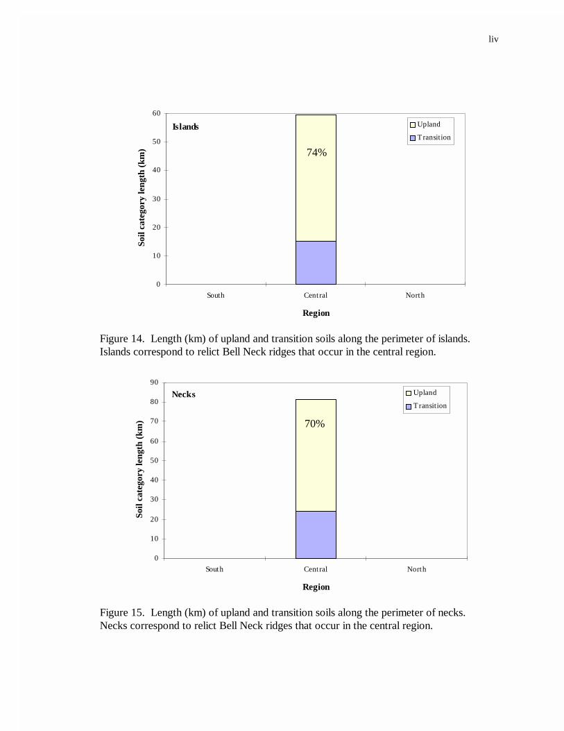
liv
Islands
0
10
20
30
40
50
60
South Central North
Region
Soi
l cat
egor
y le
ngth
(km
)
Upland
Transition
74%
Figure 14. Length (km) of upland and transition soils along the perimeter of islands.Islands correspond to relict Bell Neck ridges that occur in the central region.
Necks
0
10
20
30
40
50
60
70
80
90
South Central North
Region
Soi
l cat
egor
y le
ngth
(km
)
Upland
Transition
70%
Figure 15. Length (km) of upland and transition soils along the perimeter of necks.Necks correspond to relict Bell Neck ridges that occur in the central region.

lv
Table 7. Length of coastline (boundary between forest and marsh) and percent of eachforest soil category (transition = hydric, upland = nonhydric) along the coastline.
RegionCoastline length
(km)Transition soils
(%)Upland soils
(%)
South 45 50 45
Central 263 32 69
North 94 16 82

lvi
Creek positions and vegetation zone boundaries appeared to be in the same position for
both years compared. However, any changes involving only a few meters would not be
detectable given the large scale (1:20,000) of the older photos.
4.2 Ecosystem State Characterization
Not all vegetation zones were present at all sites. Four sites (9, 11B, JB, BFF)
lacked low marsh, six sites (5, 8, 10, 11, 12T, 21) lacked high marsh, three sites (5, 17,
27) lacked transition zone, and nine sites (10, 11B, JA, 13H, 17,18, 21B, 27, 28) lacked
forest zone. Most of the missing forest zones were due to the conversion of forest with
agriculture fields. In addition, two of the sites (5, 27) had groundwater seeps, which did
not fit the criteria for any of the four vegetation zones defined for this study.
Due to variation in the widths of vegetation zones, not all zones had the same
number of sample plots within them. In order to show within-zone variation along a
gradient from sea to land and to maintain consistency for comparing sites, data from the
high marsh and transition zones are represented by two plots. These plots are reported as
H1, H2, T1, and T2, with both number 1 plots representing zone data closer to the sea
and number 2 plots representing zone data closer to the land (see Figure 16). In order to
portray data as two plots per zone for zones where more or less than two plots were field
sampled, data were either averaged or represented twice. More specifically, zones where
there were four plots sampled, plots 1 and 2 were averaged to represent T1 or H1 and
plots 3 and 4 were averaged to represent T2 or H2. For zones where there were three

lvii
Plots sampled in the field as:
Forest Transition High Marsh Low Marsh
T1T3 T2 H2H3H4 L2 L1H1F3 F2 F1
F1F3 F2 T1T2 H1H2 L2 L1
F1F3 F2 T1T2 H1H2 L2 L1
T2F1F2F3 T1 L1L2H1Forest Transition
HighMarsh
LowMarsh
Figure 16. Method used to portray field data as two plots per zone in the high marshand transition zone. For high marsh and transition zones with four sample plots, plots 1and 2 were averaged and plots 3 and 4 were averaged. For zones with three sampleplots, plots 1 and 2 were averaged, and plots 2 and 3 were averaged. For zones withtwo sample plots, both plots were represented individually. For zones with only oneplot, that single plot was represented twice. All plots sampled in the field for the forestand low marsh zones are represented individually because they were consistently placedfor all sites and therefore are directly comparable.
Plots portrayed forzone comparison as:
Plots sampled in the field as:
Plots portrayed forzone comparison as:
lviii
plots sampled, the middle plot was averaged with both the 1st and 3rd plots. Zones that
were so narrow that only one plot was sampled showed no within-zone variation at a scale
in which I was interested. However, this single plot was represented as both the number 1
and 2 plots in order to show that its characteristics occurred next to the landward and
seaward side of that zone. All plots are represented individually for the low marsh and
forest zones because these plots were consistently placed in the field and therefore are
directly comparable. Table 8 summarizes the total number of plots sampled for each
vegetation zone.
Low marsh vegetation consisted entirely of herbaceous plants, and because it had
no shrubs or trees, it lacked measurements for tree basal area and canopy cover (Figure
17). There was a broad range in terms of vegetated ground coverage in the low marsh,
but in general, vegetative cover increased inland towards the high marsh. The mean cover
in L1 plots was 56 % and the mean cover in L2 plots was 64 %. The high marsh also was
dominated by herbaceous cover, had a few shrubs, and no trees. The high marsh had the
highest percent of herbaceous cover among the four zones and had a lower range in cover
than the low marsh. The range in herbaceous cover decreased and the number of shrubs
slightly increased in the landward plot (H2) of the high marsh. The transition zone was
moderately vegetated by herbaceous plants, had a large number of shrubs, very few trees,
and consequently low basal area and canopy cover. Herbaceous cover in the transition
and forest zones includes vines <1 m as well as nonwoody plant species. There was no
gradational change in the herbaceous cover or shrub density in the landward direction of
the transition zone. However, tree density, basal area, and canopy cover increased

lix
Table 8. Number of sample plots in each vegetation zone by site.
Number of Plots SampledSite
NumberLow
MarshHigh
Marsh Transition ForestGround-
Water Seep
2 2 4 1 3 03 2 4 1 3 05 2 0 0 3 28 2 0 1 1 09 0 3 1 3 010 1 0 3 0 011 0 0 2 1 011b 0 2 1 0 0
12JA 2 2 2 0 012JB 0 2 2 1 0BFF 0 2 2 3 0BSN 2 1 2 3 012T 2 0 1 1 013 2 1 2 2 0
13H 2 2 2 0 017 2 2 0 0 018 2 1 2 0 021 2 0 2 3 0
21B 2 2 1 0 022 1 1 3 2 026 2 1 1 3 027 2 3 0 0 228 2 1 0 0 0

lx
81014191917171816N =
Plot number
F3F2F1T2T1H2H1L2L1
He
rba
ceo
us c
ove
r (%
)
120
100
80
60
40
20
0
81014191917171816N =
Plot number
F3F2F1T2T1H2H1L2L1
Shr
ubs
(no.
/ ha
)
5,000
4,000
3,000
2,000
1,000
0 3
BFF
Figure 17. Boxplots showing physical components of vegetation structure along a gradientfrom low marsh to forest. Shrubs included Pinus and Juniperus with dbh <10 cm and allmembers of the following genera: Iva , Baccharis, Myrica, and Vaccinium. The solidcenter line indicates the median, the upper and lower edges of the box represent the 1stand 3rd quartiles, and the top and bottom whiskers represent the minimum and maximumvalues except when outliers or extremes are present. Outliers are indicated with opencircles and represent cases with values between 1.5 - 3.0 box lengths from the upper orlower box edge. Extremes are indicated with a star and represent cases with values >3.0box lengths from the upper or lower box edge. Outliers and extremes are labeled withtheir corresponding site number.
11B 11B
3
10
512JA13H
21B 1121B
13 5

lxi
Figure 17. Continued
81014191917171816N =
Plot number
F3F2F1T2T1H2H1L2L1
Tre
e d
ens
ity (
no./
ha) 4,000
3,000
2,000
1,000
0
81014191917171816N =
Plot number
F3F2F1T2T1H2H1L2L1
Ba
sal a
rea
(m
^2/
ha) 40
30
20
10
0
11
JB
BFF
11
11B
81014191917171816N =
Plot number
F3F2F1T2T1H2H1L2L1
Tre
e c
ano
py
cove
r (%
)
100
80
60
40
20
0
9
3
12JB 11B
BFF12JB
9
11

lxii
landward towards the forest. The herbaceous stratum was sparse and shrub density was
low in the forest zone. Instead this zone was dominated by trees with an average basal
area of 17 m2/ha and canopy cover of 58 %. In a landward direction within the forest, tree
density decreased, basal area decreased in range, and canopy cover increased.
There were several outliers and extremes in each physical structure component of
the vegetation. Although several sites deviated from others for a single component in a
single plot or zone; a few sites exhibited several abnormalities. Site 11B had a consistently
higher herbaceous cover in its high marsh zone and had a higher than average density and
basal area in its T1 plot. Sites 12JB and BFF had higher tree densities and basal area in
their transition zones. Moreover, BFF had a higher shrub density in its F1 plot. Finally,
site 11 had a lower herbaceous cover in its T2 plot and a higher than normal tree density
and basal area in its transition zone.
Species richness increased from the low marsh to the forest; with a total of 44
species found among all plots sampled (Table 9). Of these species, only 5 were found in
the low marsh, 17 in the high marsh, 23 in the transition, and 34 in the forest plots. Table
10 summarizes the relative percent ground cover of each of these species, and Table 11
lists the importance values for woody species. Importance values (IV) were calculated
differently for the forest and the other three zones because basal area is relatively low in
the first three zones and much higher in the forest. For the low marsh, high marsh, and
transition zones, IVs are equivalent to the average relative density for species >1m. Forest

lxiii
Table 9. Plant species present in the four vegetation zones. Presence is indicated by an Xand species are listed below their family name. Species nomenclature follows Radford etal. (1968).
Family SpeciesLow
marshHigh
marsh Transition ForestPoaceae Spartina alterniflora X X X Spartina patens X X X Distichlis spicata X X X X Panicum virgatum X X X Setaria viridis X X X Phragmites australis X XJuncaceae Juncus roemerianus X X X Juncus gerardi X XCyperaceae Scirpus sp. X XPlumbaginaceae Limonium carolinium X X X XChenopodiaceae Salicornia spp. X X X Atriplex patula X X XTyphaceae Typha sp. XAsclepiadaceae Asclepias incarnata X XApiaceae Hydrocotyle sp. XAnacardiaceae Rhus radicans X XBignoniaceae Bignonia capreolata XVitaceae Parthenocissus quinquefolia X X Vitis sp. XLiliaceae Smilax bona-nox X Smilax rotundifolia XEricaceae Vaccinium corymbosum X

lxiv
Table 9. Continued
Family SpeciesLow
marshHigh
marsh Transition ForestAsteraceae X X X Iva frutescens Baccharis halimifolia X X Erechitites hieracifolia X Borrichia frutescens XMyricaceae Myrica cerifera X XCupressaceae Juniperus virginiana X X XPinaceae Pinus taeda X X Pinus serotina X XRosaceae Prunus serotina XAquifoliaceae Ilex opaca X Ilex sp. XAceraceae Acer rubrum XNyssaceae Nyssa sylvatica XUlmaceae Celtis occidentalis XHamamelidaceae Liquidambar styraciflua XLauraceae Persea borbonia XAraliaceae Aralia spinosa XOleaceae Ligustrum sp. XFagaceae Quercus phellos X Quercus falcata XMagnoliaceae Liriodendron tulipifera X Magnolia virginiana XTOTALS 44 5 17 23 34

lxv
Table 10. Relative percent ground cover (0-1m) of species or other cover type in eachvegetation zone. Species without at least 1% relative cover were not reported.
Plot Number
Cover Type or Species L1 L2 H1 H2 T1 T2 F1 F2 F3
n = 48 54 63 63 60 60 42 30 24
Spartina alterniflora 43 48 2 3 1 1Spartina patens 1 7 40 38 22 22Distichlis spicata 4 12 28 27 10 7Salicornia spp. 6 3Borrichia frutescens 1Juncus geradi 3 3 7Iva frutescens 5 5 18 14Setaria viridis 1 1 2 1Limonium carolinium 1 1 1 1Juncus roemerianus 7 15 4 4 1Baccharis halimifolia 1 1 4Panicum virgatum 4 7 1 5 1Phragmites australis 1 1Typha sp. 1 1Myrica cerifera 3 3 5 1 1Juniperus virginiana 1 3Pinus taeda 2 2 4Erechtites hieracifolia 2Liquidambar styraciflua 1 1Rhus radicans 4 4 2Bignonia capreolata 2 3 6Smilax bona-nox 3 6 2Asclepias incarnata 1 1unidentified graminoid 2 1Persea borbonia 1 1Atriplex patula 1Smilax rotundifolia 1Quercus phellos 1Ilex opaca 1Celtis occidentalis 1Hydrocotyle sp. 1Parthenocissus quinquefolia 1Vitis sp. 1

lxvi
Table 10. Continued
Plot Number
Cover Type L1 L2 H1 H2 T1 T2 F1 F2 F3
Bare ground 38 30 5 3 7 6 1 3Wrack 3 3 2 4 6 1Pothole 3 3 2 2Crab burrow 2 3Dead shrub 1 1 1Stump 1 1Dead tree 1 1 1Litter 8 15 57 67 64Woody debris 3 1 12 9 11Vegetated Total 54 70 88 92 74 68 26 24 22Unvegetated Total 46 30 11 8 26 31 73 76 78Grand Total 100 100 100 100 100 100 100 100 100

lxvii
Table 11. Importance values (IV) for woody species in the four vegetation zones forall field sites. IVs were calculated differently depending on the zone. Low marsh,high marsh, and transition IVs are equivalent to their average relative density(species >1m tall). Forest IVs were calculated by averaging relative density and basalarea for species > 1m, by plot. A sum of less salt tolerant species (LST) occurring inthe transition zone was calculated, and these species are indicated with *. All woodyspecies occurring in the high marsh were salt tolerant, and all species occurring in theforest were salt intolerant. Species without at least 1 % relative importance were notreported.
Plot Number
Species L1 L2 H1 H2 T1 T2 F1 F2 F3
n= 16 18 21 21 20 20 14 10 8
Iva frutescens 41 42 60 42Baccharis halimifolia 5 12 17 1 1Myrica cerifera* 12 14 12 3 1Juniperus virginiana* 13 19 21 2 5Pinus taeda* 4 7 33 38 34Prunus serotina 3 5 11Ilex opaca 3 9 12Nyssa sylvatica 4 10 12Celtis occidentalis 14 16 1Liquidambar styraciflua 3 1 9Liriodendron tulipifera 1 6 7Aralia spinosa 1 5 3Persea borbonia 1 2Quercus falcata 2LST species (*) 29 40Hardwood IV 0 0 0 0 0 0 29 53 59TOTAL 0 0 41 47 100 100 96 100 100

lxviii
IVs were calculated by averaging the relative density and relative basal area of each
species >1 m tall by plot.
The low marsh was dominated by a single halophytic grass species, Spartina
alterniflora, in addition to having a large portion of bare ground. Salicornia spp. and
Distichlis spicata were the next most prevalent yet neither of these covered more than an
average 6 % of the ground in the L1 plots. D. spicata was 8% higher, in average
importance, in the plots farther inland (L2). Overall, the importance of vegetated ground
cover was 16 % higher in L2 than L1.
The high marsh was dominated by S. patens and D. spicata, and the percentage of
unvegetated ground cover was low (8-11 %), relative to the low marsh (30-46 %).
Juncus roemerianus was the next most prevalent species; however, it did not cover more
than an average of 15 % of either high marsh plots. Although there were a number of
other species present in this zone, none had >5 % cover, on average. There did not
appear to be any significant differences in vegetation characteristics between the H1 and
H2 plots.
Two grasses (S. patens, D. spicata) and one shrub (Iva frutescens) were the
predominate plant species in the transition zone. The percentage of bare ground cover
was similar to the high marsh, although there was an additional type of unvegetated
ground cover in the form of leaf litter. Vegetated ground cover was 6 % lower, and
unvegetated ground cover was 6% higher in T1 than T2. The percentage of less salt
tolerant genera (Panicum, Setaria, Pinus, Juniperus) was slightly higher (8 %) in T2 than

lxix
T1, and the percentage of salt tolerant genera (Spartina, Distichlis, Juncus, Iva) was
slightly lower (8%) in T2 than T1.
The forest ground cover was composed primarily of leaf litter and woody debris
with only an average of 22-26 % vegetated cover. The species composition was rather
variable with no single species dominating. The only salt tolerant species with at least 1 %
average relative cover was L. carolinium and it was located in the most seaward forest
plot (F1).
The low marsh zone had no shrubs or trees in any plots. I. frutescens was the
most important woody species in the high marsh. However, it was not present in all high
marsh sites. I. frutescens was also the most important woody species in the transition
zone, although its degree of importance decreased landward. B. halimifolia, M. cerifera,
and J. virginiana were similar in importance for the transition, and all were more
important in T2 than T1. P. taeda had the lowest IV in the transition zone, but was
similar to J. virginiana in that it was more important in T2 plots than T1 plots. P. taeda
was the most important species in all three forest plots, and the remaining species showed
variation across the plots. J. virginiana and M. cerifera were relatively important in F1
but were very unimportant in the two landward plots. In general, hardwood species
importance increased with increasing distance from the marsh (Table 11). Specifically, C.
occidentalis showed a relative importance in both F1 and F2 but was negligible in F3. In
contrast, the hardwood tree species P. serotina, I. opaca, N. sylvatica, L. styraciflua, Q.
falcata, and L. tulipifera all increased in importance with increased distance from marsh.

lxx
With the exception of three extreme sites, the low marsh had no dead shrubs or
trees, but had stumps in its landward plot (Figure 18). The high marsh had the most dead
short shrubs (<1 m) of the four zones. Short shrub (<1 m) density was higher in the
landward plot of the high marsh. In contrast, the high marsh had very few dead trees, tall
shrubs (>1 m), or stumps. The transition zone had a low number of dead shrubs (<1 m)
but the largest number of dead shrubs (>1 m) in its seaward plot. The transition zone also
had the largest number of dead trees and was second to the forest in stump density. The
forest had no dead shrubs, and a few dead trees. Both dead tree and stump density
increased away from the marsh.
There were a number of outliers and extremes for all dead components and several
sites in particular were deviant in several zones or vegetative components. Site 12JA had
higher than average shrub (<1 m) densities in its low marsh, high marsh, and transition
zones; shrub (>1 m) densities in its high marsh zone; tree densities in its high marsh and
transition zones; and stump densities in its low marsh and high marsh zones. Site 10
differed from the average in its low marsh zone by having higher shrub (<1 m) and tree
densities. Sites 12T, 13H, 21 and 22 had higher dead shrub densities (both sizes) in their
transition zones. Furthermore, stump densities were higher for 13H in its high marsh zone
and for 12T in its transition zone. Site BFF had a higher than average dead tree density in
its high marsh zone and more stumps in its transition zone. Finally, site 12JB had a high
dead tree and stump density in its F1 plot.

60
81014191917171816N =
Plot number
F3F2F1T2T1H2H1L2L1
De
ad
shr
ubs
<1
m (
no./
ha)
2,000
1,000
0
81014181917171816N =
Plot number
F3F2F1T2T1H2H1L2L1
De
ad
shr
ubs
>1m
(n
o./h
a)
1,200
1,000
800
600
400
200
0
81014191917171816N =
Plot number
F3F2F1T2T1BH2H1L2L1
De
ad
tre
e d
ens
ity (
no./
ha)
2,000
1,500
1,000
500
0
81014191917171816N =
Plot number
F3F2F1T2T1H2H1L2L1
Stu
mp
s (n
o./
ha)
1,600
1,400
1,200
1,000
800
600
400
2000
Figure 18. Boxplots showing dead vegetation components along a gradient from low marsh to forest. Boxplot components aredescribed in Figure 17.
10, 12JA
12JA
21B
21
2113H22JA12T
2
27
12JA
26 26
12JA
27
22
22
BSN, 1821
12T, 13H, 18
10, BSN 12JA BFF
212JA
13H
12JA
12JA11
12JB
12JA2
BSN
12JA 12JA 13H
12T, BFF
BSN
17
12JB

61
All low marsh zones were mapped as Chincoteague soils, but soil profile
descriptions showed that not all sites were identical in the field (Table 12). Most (78 %)
of the low marsh soils had an organic rich horizon, and 71 % of these had O horizons >30
cm deep. The depth of the organic rich horizon ranged from 0 to >100 cm in both the L1
and L2 sample plots; however, the median was lower by almost 40 cm in the landward
plot (L2) (Figure 19). The extent of decomposition in the low marsh O horizon ranged
from low (fibric peat) to high (sapric muck). The range in percent organic matter content
was similar for the soil surface and subsurface (2 - 43 %), but the median was much lower
for the subsurface soils (Figure 20). For all sites, low marsh soils had indicators of
reduced conditions (i.e. chromas < 2) and soils at six of the sites were mottled. The only
noticeable difference between low marsh soils forming adjacent to different forest soil
types was that the few sites with a B horizon, in the upper 40 cm, were located next to
forests with nonhydric soils. The texture of the mineral soil ranged from loamy sand to
sandy clay, although most of the soils were predominately loamy. The low marsh had the
highest salinities of the four vegetation zones (Figure 21). Salinity range was similar for
the soil surface (6-36 ppt) and subsurface (2-29 ppt), but the salinity median of the
subsurface soil was much lower.
Most high marsh soils were mapped as Magotha, but there were three sites that
lacked this hydric soil series and still had the high marsh zone. Two of these sites (BSN,
26) had a very narrow (<9 m) high marsh zone. There were a total of sixteen sites with
high marsh, and all but four of these had an organic rich horizon (Table 13). Within the
high marsh, the depth of the O horizon ranged from 3 to >100 cm, and did not differ

62
Table 12. Low marsh soil profile characteristics. Values for mottle abundance range from 1-3 with 3 representing the mostmottles.
MapSoil
Series
ForestSoil
Series
Site # Horizon Depth(cm)
Texture orDegree of
Decompositon
MatrixHue/Value/Chroma
MottleHue/Value/Chroma
MottleAbundance
OrganicMatter
(%)
Salinity(ppt)
ChA NmA 2 A 0 - 30 Sandy loam 10YR 4/1 10YR 6/8 3 7.9 15.0E 30 - 60 Loamy sand 10YR 6/2 10YR 5/1 3 2.9 6.3
10YR 6/4 33 A 0 - 40 Silt 5B 4/1 21.9 20.0
O 40 - 70 Fibric peat 10YR 3/1 30.2 21.210 O/A 0 - 15 Sandy loam 10YR 3/1 11.9 15.8
A 15 - 40 Sandy clay 5B 4/1 10YR 3/1 3 1.9 2.421 O1 0 - 20 Fibric peat 10YR 3/2 47.3 18.3
O2 20 - 90 Sapric muck 10YR 3/2 41.2 17.4A 90 - 100 Silty loam 10YR 2/0
DrA 22 O/A 0 - 60 Peaty Silt 2.5G 2/0 24.0 19.2A 60 - 80 Loam 2.5G 2/0 16.4 14.4E 80 - 100 Loam 10YR 4/1
26 O1 0 - 50 Fibric peat 10YR 3/2 45.5 19.1O2 50 - 90 Sapric muck 10YR 2/0 38.7 21.7A 90 - 100 Loam 10YR 2/1
MuA BSN O 0 - 10 Fibric peat 10YR 3/2 30.9 18.1A 10 - 40 Silt loam 5B 4/1 2.2 2.7
12JA A1 0 - 15 Silty loam 10YR 4/1 10YR 5/8 3 8.4 11.810YR 2/1 3
A2 15 - 33 Silty loam 10YR 2/1 10YR 4/1 1 7.8 4.7B 33 - 50 Sandy loam 2.5Y 4/3
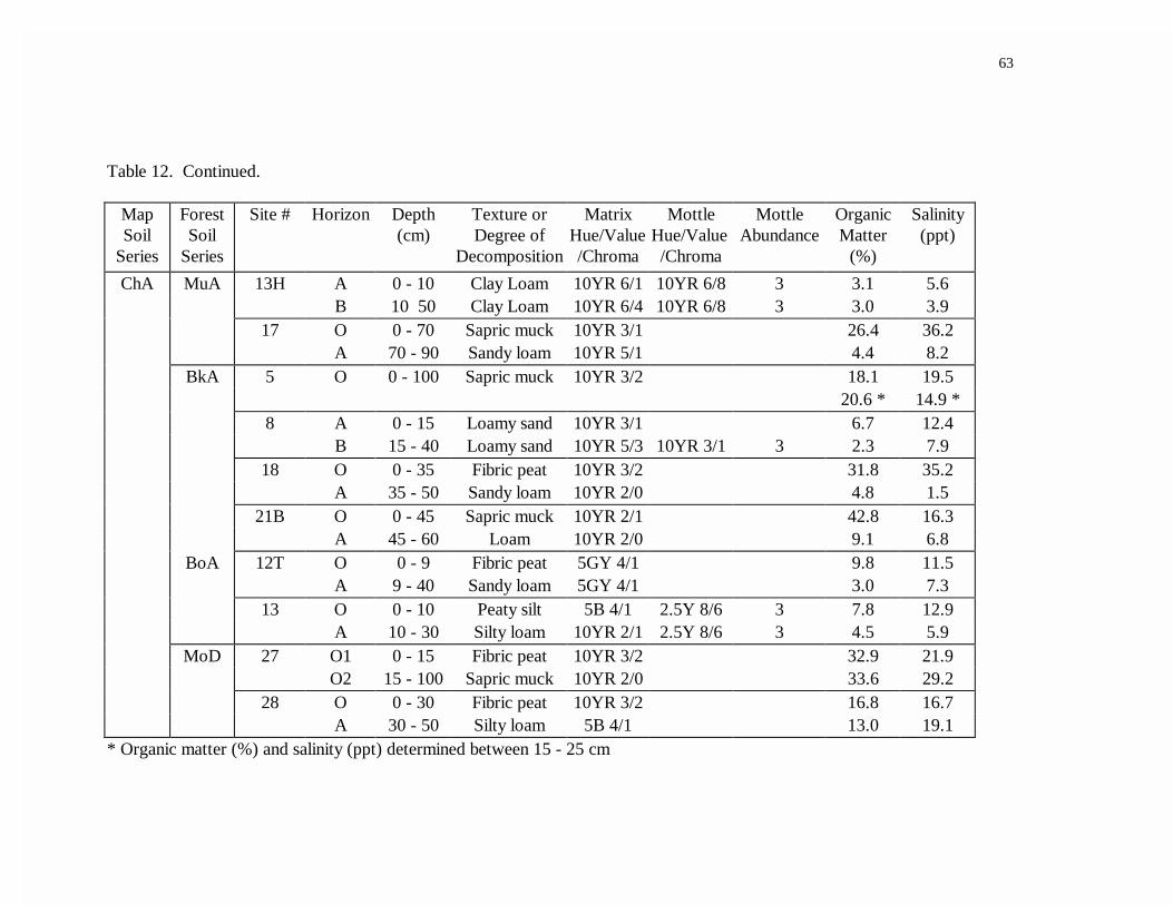
63
Table 12. Continued.
MapSoil
Series
ForestSoil
Series
Site # Horizon Depth(cm)
Texture orDegree of
Decomposition
MatrixHue/Value/Chroma
MottleHue/Value/Chroma
MottleAbundance
OrganicMatter
(%)
Salinity(ppt)
ChA MuA 13H A 0 - 10 Clay Loam 10YR 6/1 10YR 6/8 3 3.1 5.6B 10 50 Clay Loam 10YR 6/4 10YR 6/8 3 3.0 3.9
17 O 0 - 70 Sapric muck 10YR 3/1 26.4 36.2A 70 - 90 Sandy loam 10YR 5/1 4.4 8.2
BkA 5 O 0 - 100 Sapric muck 10YR 3/2 18.1 19.520.6 * 14.9 *
8 A 0 - 15 Loamy sand 10YR 3/1 6.7 12.4B 15 - 40 Loamy sand 10YR 5/3 10YR 3/1 3 2.3 7.9
18 O 0 - 35 Fibric peat 10YR 3/2 31.8 35.2A 35 - 50 Sandy loam 10YR 2/0 4.8 1.5
21B O 0 - 45 Sapric muck 10YR 2/1 42.8 16.3A 45 - 60 Loam 10YR 2/0 9.1 6.8
BoA 12T O 0 - 9 Fibric peat 5GY 4/1 9.8 11.5A 9 - 40 Sandy loam 5GY 4/1 3.0 7.3
13 O 0 - 10 Peaty silt 5B 4/1 2.5Y 8/6 3 7.8 12.9A 10 - 30 Silty loam 10YR 2/1 2.5Y 8/6 3 4.5 5.9
MoD 27 O1 0 - 15 Fibric peat 10YR 3/2 32.9 21.9O2 15 - 100 Sapric muck 10YR 2/0 33.6 29.2
28 O 0 - 30 Fibric peat 10YR 3/2 16.8 16.7A 30 - 50 Silty loam 5B 4/1 13.0 19.1
* Organic matter (%) and salinity (ppt) determined between 15 - 25 cm

64
81014191917171816N =
Plot number
F3F2F1T2T1H2H1L2L1
Org
ani
c ho
rizo
n d
ep
th (
cm)
0
-20
-40
-60
-80
-100
-120
21
27327
Figure 19. Boxplots showing depth of the organic rich horizon (cm) in each sample plot.Boxplot components are described in Figure 17.

65
14181618N =
Zone
ForestTransitionHigh marshLow marsh
Org
ani
c m
atte
r (%
) 70
60
50
40
30
20
10
0
212JB
2
14181618N =
Zone
ForestTransitionHigh marshLow marsh
Org
ani
c m
atte
r (%
) 60
50
40
30
20
10
0
12JB
22
27
Figure 20. Boxplots showing the organic matter (%) of the soil (A) 0-10 cm and (B)subsurface (first 10 cm of the next deeper horizon), for each vegetation zone. Boxplotcomponents are described in Figure 17.
(B) Subsurface

66
14181618N =
Zone
ForestTransitionHigh marshLow marsh
Sa
linity
(p
pt)
40
30
20
10
0
14181618N =
Zone
ForestTransitionHigh marshLow marsh
Sa
linity
(p
pt)
40
30
20
10
0
Figure 21. Boxplots showing salinity (ppt) of the soil (A) 0 - 10 cm and (B) subsurface(first 10 cm of the next deeper horizon), for each vegetation zone. Boxplot componentsare described in Figure 17.
(B) Subsurface
27
11 12JB21B

67
Table 13. High marsh soil profile characteristics. Values for mottle abundance range from 0-3 with 3 representing the mostmottles.Map Soil
SeriesForestSoil
Series
Site # Horizon Depth(cm)
Texture or Degreeof Decomposition
MatrixHue/Value/
Chroma
MottleHue/Value/Chroma
MottleAbundance
OrganicMatter
(%)
Salinity(ppt)
ChA NmA 9 O 0 - 45 Sapric muck 10YR 3/2 54.3 9.2A 45 - 60 Sandy loam 10YR 2/1 10.8 6.6
DrA 26 O 0 - 15 Fibric peat 10YR 3/2 61.9 14.6A 15 - 40 Sand 10YR 5/1 4.9 2.9
MuA BSN O 0 - 10 Sapric muck 10YR 3/2 15.1 14.6A 10 - 40 Silty loam 10YR 3/1 5.8 6.0
MaA NmA 2 O 0 - 8 Fibric peat 10YR 3/1 21.7 10.2A 8 - 20 Sandy loam 10YR 2/1 5.8 6.1E 20 - 40 Loamy sand 10YR 6/2 10YR 6/4 3
3 O 0 - 40 Fibric peat 10YR 3/1 24.6 23.6O/A 40 - 50 Peaty loam 10YR 3/1 18.8 8.0A 50 - 60 Sandy clay loam 10YR 2/1
12JB O 0 - 11 Fibric peat 10YR 3/1 47.6 8.8A 11 - 30 Silty clay 10YR 2/1 10YR 6/1 1 24.8 7.2
BFF O 0 - 10 Fibric peat 10YR 3/2 33.7 12.4A 10 - 20 Silty loam 10YR 2/1 10YR 5/1 1 15.7 4.2E 20 - 40 Silty loam 10YR 5/1
DrA 11B O 0 - 40 Fibric peat 10YR 3/2 59.5 21.1A 40 - 60 Silty loam 10YR 4/1 10.2 7.3
22 O/A 0 - 30 Peaty silt 2.5G 2/0 10YR 2/1 2 15.8 14.4A 30 - 70 Silt 2.5G 2/0 10YR 2/1 2 13.4 11.3

68
Table 13. Continued.Map Soil
SeriesForestSoil
Series
Site # Horizon Depth(cm)
Texture or Degreeof Decomposition
MatrixHue/Value/
Chroma
MottleHue/Value/Chroma
MottleAbundance
OrganicMatter
(%)
Salinity(ppt)
MaA MuA 13H A 0 - 10 Loam 10YR 3/1 9.3 7.1E 10 - 40 Loam 10YR 6/1 10YR 6/3 3 3.4 2.5
17 A1 0 - 10 Sandy loam 10YR 5/1 2.5 0.9E 10 - 30 Sandy loam 2.5Y 6/2 1.9 0.8B 30 - 50 Sandy loam 2.5Y 6/4
BoA 13 O 0 - 3 Peaty loam 10YR 2/2 12.2 6.2A 3 - 15 Loam 10YR 4/1 10YR 2/1 2 5.1 4.0E 15 - 40 Loam 10YR 6/1 2.5Y 6/8 3
BkA 18 O 0 - 20 Fibric peat 10YR 3/2 42.0 21.3A 20 - 35 Sandy loam 10YR 2/1 6.0 5.7B 35 - 50 Sandy loam 10YR 6/3 10YR 2/1 3
21B A 0 - 25 Sandy loam 10YR 2/1 8.6 3.3B 25 - 40 Sandy loam 2.5Y 6/6 10YR 2/1 1 1.9 5.8
MoD 27 O1 0 - 15 Fibric peat 10YR 3/2 50.2 8.7O2 15 - 100 Sapric muck 10YR 2/0 47.8 16.9
28 A 0 - 15 Sandy loam 10YR 4/2 5.4 2.6B 15 - 40 Sandy clay loam 10YR 6/4 10YR 4/2 2 1.9 1.2

69
much along the sea to land gradient (Figure 19). The degree of the decomposition in the
O horizon of high marsh soils varied from low (fibric) to high (sapric) as did percent
organic matter in both the soil surface (2.5 - 62 %) and soil subsurface (2 - 48 %)
horizons (Figure 19). High marsh soils at all sites sampled displayed signs of reduced
conditions (chroma <2) and soils at nine of the sites were mottled. Four of the sites had B
horizons within 35 cm of the soil surface and all of these occurred in marshes adjacent to
uplands. The texture of the mineral soil ranged from sand to sandy clay loam; however,
the majority of the soils were predominately loam. Soil salinity of the high marsh was
lower than in the low marsh but higher than the other two zones. Salinity ranged from
0.9-23.6 ppt in the soil surface and from 0.6-16.9 in the subsurface (Figure 21). With
exception for site 18, high marsh zones forming seaward of uplands had lower salinities
than those forming seaward of wetlands.
Transition vegetation zones were present at 18 sites, and most (13) of these
developed over the transition between the MaA and forest soil series (Table 14). Fifty
percent of the transition sites had soils with organic rich horizons; however, the depth of
the horizon was much shallower than those in either the low or high marsh zones (Figure
19). There was no change in O horizon depth from the T1 to T2 plot. Similar to the
other two marsh zones, the degree of decomposition varied from low to high (fibric peat
to sapric muck). Percent organic matter of the soil was lower for the transition zone (14.8
% surface average) than the other two marsh zones, and this percentage decreased in the
soil’s subsurface to an average of <5 %. Soils at all of the sites had indicators of reduced
conditions (chroma <2) and soils at 50 % of the sites were mottled. Nine of the sites had

70
Table 14. Transition soil profile characteristics. Values for mottle abundance range from 0 - 3 with 3 representing the mostmottles.
MapForest- Marsh
Soil Series
Site # Horizon Depth(cm)
Texture or Degreeof Decomposition
MatrixChroma
MatrixHue/Value/
Chroma
MottleHue/Value/
Chroma
OrganicMatter
(%)
Salinity(ppt)
NmA 11 A 0 - 15 Sandy loam 10YR 4/1 7.5 2.6E 15- 40 Sandy loam 10YR 5/2 10YR 4/1 1 3.6 0.9
NmA - MaA 2 O 0 - 6 Fibric peat 10YR 3/1 45.7 1.5A 6 - 21 Sandy loam 10YR 4/1 7.6 0.7B 21 - 40 Sandy loam 10YR 6/3 10YR 4/1 3
3 O 0 - 5 Fibric peat 10YR 3/1 14.9 1.6A 5 - 20 Sandy loam 10YR 5/1 10YR 6/8 1 3.0 0.4B 20 - 40 Sandy loam 10YR 6/6 10YR 6/8 2
10 A 0 - 15 Sandy loam 10YR 4/1 2.5 Y6/2 1 4.5 1.4E 15 - 40 Sandy loam 2.5 Y6/2 10YR 6/8 3 2.2 1.0
12JB O 0 - 6 Fibric peat 10YR 2/1 28.9 4.6A 6 - 20 Silt loam 10YR 2/1 10YR 5/1 2 8.1 1.1E 20 - 40 Loam 10YR 6/1 10YR 4/4 3
BFF A 0 - 8 Silt loam 10YR 3/1 11.0 1.1E 8 - 30 Silt loam 10YR 5/1 3.6 0.6
21 O 0 - 10 Mucky sandy loam 10YR 4/1 17.5 7.8A 10 - 40 Sandy loam 10YR 4/1 3.9 1.7
NmA - ChA 9 O 0 - 5 Fibric peat 10YR 3/2 15.0 2.7A 5 - 35 Sandy loam 10YR 4/1 2.9 0.7E 35 - 50 Loamy sand 10YR 6/1
DrA - MaA 11B O 0 - 5 Peaty loam 10YR 3/1 26.0 2.7A 5 - 40 Loam 10YR 4/1 10YR 6/4 3 5.2 1.0

71
Table 14. Continued.Map
Forest- MarshSoil Series
Site # Horizon Depth(cm)
Texture or Degreeof Decomposition
MatrixChroma
MatrixHue/Value/
Chroma
MottleHue/Value/
Chroma
OrganicMatter
(%)
Salinity(ppt)
DrA - MaA 22 A 0 - 15 Silt loam 10YR 3/1 9.6 8.2B1 25 - 35 Silt loam 2.5Y 5/4 2.8 0.8B2 35 - 50 Sand 2.5Y 5/4
DrA - ChA 26 O 0 - 10 Sapric muck 10YR 3/2 18.2 2.7A 10 - 15 Loamy sand 10YR 4/2 7.5 0.4E 15 - 40 Loamy sand 10YR 5/1
MuA - MaA 13H O 0 - 3 Sapric muck 10YR 2/1 10.9 0.8A 3 - 10 Loam 10YR 4/1 2.6 0.6B 10 - 40 Loam 2.5Y 6/4
MuA - ChA BSN A 0 - 10 Sandy silt loam 10YR 4/1 5.1 2.0B 10 - 30 Sandy silt loam 10YR 4/3 1.9 1.0
BoA - MaA 12T A 0 - 40 Fine sandy loam 10YR 3/2 13.3 4.4B 40 - 50 Fine sandy loam 2.5Y 6/4 10YR 2/1 1 6.2 1.2
13 O 0 - 4 Sapric muck 10YR 2/2 11.1 1.9A 4 - 15 Sandy loam 10YR 4/1 10YR 2/1 1 3.4 1.3E 15 - 40 Sandy loam 10YR 6/1 2.5Y 6/6 2
BkA - MaA 18 A 0 - 15 Sandy clay loam 10YR 3/2 5.1 2.1B 15 - 40 Sandy loam 10YR 6/3 10YR 3/2 3 2.1 1.3
21B A 0 - 15 Sandy loam 10YR 3/1 5.8 2.4B 15 - 40 Sandy loam 2.5Y 6/6 1.7 2.4
BkA - ChA 8 A 0 - 8 Loamy sand 10YR 5/2 1.8 0.3B 8- 40 Sandy clay loam 10YR 5/4 2.0 0.3

72
a B horizon within 40 cm of the soil surface, but unlike the other zones, not all of these
horizons corresponded to soils forming adjacent to uplands. The texture of the mineral
soil ranged from sand to sandy clay loam; the majority of the soils were predominately
loam. Transition soil salinities were much lower than the other two marsh zones and
ranged from 0.3-8.2 ppt in the surface and from 0.3-2.4 ppt in the subsurface (Figure 21).
There was no a trend between transition soil salinity and the adjacent soil series type.
There were 14 forested sites; five of which were located on nonhydric soils (Table
15). Only six of these sites had soils with organic rich horizons; all were shallow (3 - 6
cm) and showed no variation in the depth between the three forest plots (Figure 19). The
degree of organic decomposition within this horizon was fairly low (fibric peat) for most
of the forest sites. Percent of forest soil organic matter ranged widely from 1-63 % for the
soil surface and was half of that for the subsurface (2-30 %) (Figure 20). All sites
displayed signs of reduced conditions within the A horizon at least, and eight sites had soil
mottling. Six of the sites had B horizons within 40 cm of the soil surface and most of
these occurred within nonhydric soil series. All six of these sites lacked the eluvial E
horizon. The mineral soil texture ranged from sand to silty loam, with most of the sites
being sandy loam. With exception for two sites (11, 12JB), both soil surface and
subsurface salinities were <1 ppt (Figure 21). Both sites with higher salinities had hydric
soil series.

73
Table 15. Forest soil profile characteristics. Values for mottle abundance range from 0 - 3 with 3 representing the mostmottles.
Map SoilSeries
Site # Horizon Depth(cm)
Texture MatrixHue/Value/
Chroma
MottleHue/Value/Chroma
MottleAbundance
OrganicMatter
(%)
Salinity(ppt)
NmA 2 O 0 - 6 Fibric peat 10YR 2/1 60.0 0.4A 6 - 18 Sandy loam 10YR 4/1 10YR 4/2 1 3.1 0.2B 18 - 44 Sandy loam 2.5Y 6/3 10YR 4/1 2
3 O 0 - 3 Fibric peat 10YR 3/2 6.7 0.3A 3 - 20 Sandy loam 10YR 4/1 30.3 0.3E 20 - 40 Sandy loam 10YR 6/1 10YR 6/8 3
9 O 0 - 6 Fibric peat 10YR 3/2 9.3 0.1A 6 - 40 Sandy loam 10YR 4/1 4.1 0.2
11 A 0 - 10 Sandy loam 10YR 2/1 20.7 4.7E 10 - 40 Sandy loam 10YR 5/2 5.8 1.3
12JB O 0 - 6 Fibric peat 10YR 3/1 62.7 1.7A 6 - 15 Silt loam 10YR 2/1 11.4 1.2E 15 - 40 Loam 10YR 5/1 10YR 2/1 2
BFF A 0 - 8 Silt loam 10YR 2/1 24.2 0.8E 8 - 35 Silt loam 10YR 5/1 10YR 6/3 1 4.3 0.4
21 O 0 - 4 Fibric peat 10YR 3/2 6.5 0.2A 4 - 10 Sandy loam 10YR 3/1 2.3 0.3E 10 - 40 Sandy loam 10YR 5/2 10YR 5/4 2
DrA 22 A 0 - 10 Loam 10YR 4/1 10YR 4/3 2 6.6 0.3B 10 - 50 Loam 10YR 4/2 10YR 4/3 2 2.7 0.6
Table 15. Continued.

74
Map SoilSeries
Site # Horizon Depth(cm)
Texture orDegree of
Decomposition
MatrixHue/Value/
Chroma
MottleHue/Value/Chroma
MottleAbundance
OrganicMatter
(%)
Salinity(ppt)
DrA 26 O 0 - 5 Fibric peat 10YR 3/2 1.2 0.6A 5 - 10 Loamy sand 10YR 4/2 10YR 6/8 3 3.1 0.1E 10 - 40 Loamy sand 10YR 6/2 10YR 6/8 3
MuA BSN A 0 - 6 Loam 10YR 4/1 13.1 0.1B 6 - 40 Loam 10YR 4/3 3.7 0.2
BkA 5 A 0 - 10 Sand 10YR 5/1 1.9 0.1B 10 - 40 Sand 10YR 5/4 2.2 0.1
8 A 0 - 8 Sand 10YR 4/2 5.0 0.1B 8 - 30 Sand 10YR 5/3 3.0 0.1
BoA 12T A 0 - 20 Sandy loam 10YR 3/2 21.3 0.3B 20 - 40 Sandy loam 10YR 5/4 3.0 0.2
13 A 0 - 15 Sandy loam 10YR 3/2 17.5 0.1E 15 - 40 Sandy loam 2.5Y 6/2 2.5Y 6/6 3 2.3 0.1

75
Marsh potholes were present in both marsh zones and the transition but not the
forest. Within zones, pothole formation was limited to sites where organic matter
accumulated. However, not all sites with organic matter accumulation had marsh
potholes. Two low marsh sites (21, 26), four high marsh sites (2, 3, 9, BFF), and one
transition site (21) had marsh potholes within study plots. I observed potholes in low
marsh site 27, and high marsh sites 11B and 27 but these potholes were not within the
study plots. Pothole depth was limited to the depth of organic matter, but did not always
penetrate as deeply as the organic matter.
Relative elevations of each sample point, determined using the laser level, were
used to calculate slope and elevation differences along various positions within the site.
The slope between L2 and F1 and the elevation difference between F1 and the average
elevation of the high marsh, or the elevation of L2 for sites lacking a high marsh zone, had
strong correlations to F1’s elevation above MSL (Figure 22). These two variables were
used to develop a multiple regression equation to predict F1’s elevation above MSL
(Figure 23) for sites lacking a permanent bench mark (Table 3). The multiple regression
equation showed a stronger relationship (R2 = 0.87) than either of the two predictor
variables alone. Site 18 was the only site that lacked GPS data and a relative F1 elevation,
and therefore none of its plots were related to MSL.
Predicted F1 values were used to tie the remainder of the plot elevations intoMSL. Adding the predicted elevations to the actual elevation data set increased the
variation a lot in the F3 plot but had little effect on the other plots (Figure 24). Elevation

76
Elevation (m) difference F1 - high marsh
1.21.0.8.6.4.20.0
Act
ual e
leva
tion
(m)
of F
1
1.8
1.7
1.6
1.5
1.4
1.3
1.2
1.1
13H13
12T
BSN
BFF
12JB
8
5
32
Slope between F1 and L2
.08.06.04.020.00-.02
Act
ual e
leva
tion
(m)
of F
1
1.8
1.7
1.6
1.5
1.4
1.3
1.2
1.1
13H13
12T
BSN
BFF
12JB
8
5
32
Figure 22. Scatter plots showing the relationship between F1’s actual elevation and (A)the elevation difference between F1 and the average high marsh elevation, or L2 where thehigh marsh zone was absent, and (B) the slope between L2 and F1. Actual elevation is theelevation relative to MSL. Each point is labeled with its associated site.
A)
r = 0.92
B)
r = 0.82

77
Actual elevation (m) of F1
1.81.71.61.51.41.31.21.1Pre
dict
ed
ele
vatio
n (m
) o
f F 1.8
1.7
1.6
1.5
1.4
1.3
1.2
1.1
13H1312T BSN
BFF
12JB
8
5
32
Figure 23. The relationship between predicted and actual elevations of F1. Actualelevations were determined using a GPS unit. Predicted elevations were determined usingthe following multiple regression equation:
predicted elevation = 0.9837(X1) - 4.1254(X2) + 0.9667
whereX1 = the difference in elevation between F1 and the average elevation of the high marsh zone, or L2 where the high marsh zone was absent, andX2 = the slope between L2 and F1.Each point is labeled with its associated site.
R2 = 0.87p= 0.0008

78
5610121299109N =
Plot number
F3F2F1T2T1H2H1L2L1
Ele
vatio
n (m
)
3.0
2.5
2.0
1.5
1.0
.5
0.0
5
81019181816161715N =
Plot number
F3F2F1T2T1H2H1L2L1
Ele
vatio
n (m
)
3.0
2.5
2.0
1.5
1.0
.5
0.0
17
Figure 24. Boxplots showing (A) actual elevation (m) above MSL and (B) actual andestimated elevation (m) above MSL, along a gradient from low marsh to forest. Actualelevations are reported for sites with GPS data and estimated elevations are reported forsites lacking GPS data. Estimated elevations were calculated using the multiple regressionequation shown in Figure 23. Boxplot components are described in Figure 17.
(B)
(A)

79
increased from low marsh to forest and was relatively similar within each zone (Table 16).
Within-zone variation was highest for the forest and transition, and lowest for the high
marsh. An overlap in elevation range existed between all zones. In general, the lower 25
% of each zone’s sites overlapped in elevation with the more seaward zone and the upper
25 % of each zone’s sites overlapped in elevation with the more landward zone (Figure
24). Between zone variation was largest between the forest and transition, with 0.38 m
difference between the averages of each zone, and 0.245 m difference between F1 and the
transition zone. Between zone variation was smallest between the transition and high
marsh, with only 0.189 m separating them on average.
Two sites (5 and 27) had a similar zone that did not meet the criteria for any of the
four described zones. For both sites, this zone appeared to be receiving groundwater
discharge and hence will be referred to as a groundwater seep. For both sites, the
groundwater seep was just seaward of the forest state. In terms of physical structure
components, percent herbaceous cover in this zone was lower than the other marsh zones,
there were a few shrubs for site 27 and none for site 5, and there were no trees at either
site (Table 17A). Site 5 had low canopy cover due to shading by trees in the adjacent
forest. Ground cover was dominated by Phragmites australis (44%) in site 5 and a fairly
high proportion (29%) was unvegetated. In site 27, ground cover was distributed among
three species (Scirpus sp., Limonium carolinium, and Hibiscus sp.), and this site, too, had
a high portion of unvegetated ground cover (Table 17B). The typical marsh species (S.
alterniflora, S. patens, D. spicata, or J. roemerianus) were rare in the groundwater seeps
and the shrub I. frutescens was absent.

80
Table 16. Elevation averages for plots and zones, and elevation differences within plotsand between zones. In order to illustrate the effects estimated elevations had on the dataset variation, variables are shown for sites with GPS data and then for all sitescombined. Average zone elevations were determined using each plot individually rather than high marsh and transition plot averages.
GPS Sites Only All Sites
Plot#
Averageplot
elevation(m)
Withinzone
difference(m)
Averagezone
elevation(m)
Betweenzone
difference(m)
Averageplot
elevation(m)
Withinzone
difference(m)
Averagezone
elevation(m)
Betweenzone
difference(m)
L1 0.695 0.6890.044 0.717 0.032 0.705
L2 0.739 0.7210.231 0.210
H1 0.940 0.9030.015 0.948 0.026 0.915
H2 0.955 0.9290.177 0.189
T1 1.101 1.0810.047 1.125 0.042 1.104
T2 1.148 1.1230.383 0.380
F1 1.374 1.3490.139 0.144
F2 1.513 1.508 1.493 1.4840.123 0.116
F3 1.636 1.609

81
Table 17. Vegetation characteristics (A) physical structure, and (B) relative %ground cover (0-1m) and species IVs for groundwater seeps. Relative % cover iscalculated same as Table 10 and IVs are calculated same as Table 11.
(A)Physical Structure Site 5 Site 27
Herbaceous cover (%) 59 46Shrub density (no./ha) 0 1,061Tree density (no./ha) 0 0Basal area (m2/ha) 0 0
Tree canopy cover (%) 9* 0* canopy cover from adjacent forest zone
(B) Ground Cover % Importance Value
Cover Type or Species Site 5 Site 27 Site 5 Site 27
Spartina alterniflora 5Spartina patens 5 2Distichlis spicata 5Phragmites australis 44Scirpus sp. 23Limonium carolinium 17Bignonia capreolata 2Hibiscus sp. 11 70Baccharis halimifolia 30Bare ground 29 43Litter 12Vegetated Total 59 57Unvegetated Total 41 43Grand Total 100 100 0 100
82
The elevations of the two groundwater seeps were higher than those of the low
marsh, and lower than those of the high marsh, on average (Table 18). The slope was
fairly steep at site 5 and very steep at site 27. For both sites, the groundwater seep
occurred seaward of a very steep forest slope and was between 0.743 m and 0.818 m
lower than the F1 plot. The groundwater seeps were not elevated much above the
adjacent seaward state.
These seeps occurred in Magotha soils that were comprised in large part of
organic matter (Table 18). Organic matter penetrated deep beneath the ground surface
and was highly decomposed (sapric muck). Salinity was low (<3 ppt) in the seeps for both
sites but was high for both sites in the next seaward zone (site 5, 19.5 ppt; site 27, 8.7 ppt)
(Tables 12 and 13).
4.3 Ecosystem State Classification
The sum of scores for the four variables used to describe the ability of the forest to
resist state change to marsh (Table 4) was used to classify forest sites into three resistance
groups: low (L), intermediate (I), and high (H). Sites with total scores between 0-2 were
classified as low resistance; sites with total scores between 3-5 were classified as
intermediate resistance; and sites with total scores of 6 or 7 were classified as high
resistance. Based on the scoring procedure, seven forest sites were classified into the L
resistance group; eight forest sites were classified into the I resistance group; and four
forest sites were classified into the H resistance group (Table 19). The ranking procedure

83
Table 18. Elevation, zone width, and soil characteristics for groundwater seeps.
Site 5 Site 27
Elevations and Zone Widths
Elevation (m) 0.803 0.880Zone slope 0.017 0.029Elevation below adjacentforest (m)
0.743 0.818
Elevation above adjacentseaward zone (m)
0.148 0.053
Zone width (m) 24 15
Soil CharacteristicsDepth of organic matter (cm) 60 65Organic matter (%) Surface (0-10cm) 20 43 Subsurface (10-20cm) 34 20Salinity (ppt) Surface (0-10cm) 2.9 1.4 Subsurface (10-20cm) 3.0 0.7Soil Series MaA MaAO horizon depth (cm) 100 100Degree of decomposition 0 - 10 cm Sapric muck Fibric peat 10 - 100 cm Sapric muck Sapric muckSoil hue/value/chroma 10YR 3/2 10YR 2/1

84
provided similar results to the scoring procedure in that sites with the lowest ranks (5-24)
corresponded to sites with the lowest scores, and sites with the highest ranks (45-55)
correspond to sites with the highest scores (Table 19). Principal components analysis
(PCA) verified the classification scheme. All sites in a given resistance group were plotted
in close proximity to each other except for site 26 (Figure 25). PCA results indicated that
site 26 was physically more similar to I sites than H sites. However, I chose to leave site
26 in the H group because it met the criteria I had defined for high resistance sites.
The three forest resistance groups were fairly distinct from each other for all four
classification variables. L forest sites had the lowest elevations above MSL, the smallest
elevation differences above their adjacent seaward zones, the flattest slopes, and were
predominately located on hydric soils (Figure 26). I sites had intermediate elevations
above MSL, intermediate elevation differences above their adjacent zones, intermediate
slopes, and were predominately located on nonhydric soils (Figure 26). H sites had the
highest elevations above MSL, the largest elevation differences above their adjacent
seaward zones, the steepest slopes, and were almost all located on nonhydric soils (Figure
26).
High marsh sites were also classified into three resistance groups: low (L),
intermediate (I), and high (H) using the sum of scores for the five variables that describe
high marsh resistance to state change to low marsh (Table 5). High marsh sites with total
scores between 0-2 were classified as L resistance; high marsh sites with scores between
3-5 were classified as I resistance; sites with scores between 5-7 were classified as H

85
Table 15. Forest scores and ranks by resistance group: low (L), intermediate (I), and high (H).
Resistance group Site ID
Soil Series Hydric = 0,
Nonhydric = 1
SCORE
Elev. above MSL (m)
0-1.25=0, 1.25-1.40=1,
>1.40=2
SCORE
RANK
Slope (F1:L2)
<0.01 = 0, 0.01-0.02=1,
>0.02=2
SCORE
RANK
Elev. above Seaward Zone (m) <0.15=0,
0.15-0.30=1, >0.30=2
SCORE
RANK
Total Score
Total Rank
L BFF NmA 0 1.16 0 3 0.0010 0 1 -0.01 0 1 0 59 NmA 0 0.97 0 1 0.0016 0 3 0.10 0 3 0 7
12JB NmA 0 1.28 1 8 0.0013 0 2 0.14 0 5 1 152 NmA 0 1.17 0 5 0.0054 0 5 0.18 1 8 1 183 NmA 0 1.19 0 7 0.0026 0 4 0.29 1 11 1 22
21B BkA 1 1.17 0 6 0.0071 0 6 0.15 1 7 2 1911 NmA 0 1.38 1 10 0.0177 1 12 0.08 0 2 2 24
I 13H MuA 1 1.43 2 13 0.0084 0 7 0.11 0 4 3 2412T BoA 1 1.33 1 9 0.0348 2 17 0.14 0 6 4 3222 DrA 0 1.54 2 16 0.0110 1 8 0.26 1 9 4 3321 NmA 0 1.39 1 11 0.0146 1 10 0.38 2 15 4 36
BSN MuA 1 1.41 2 12 0.0146 1 9 0.29 1 12 5 3317 MuA 1 1.16 0 4 0.0290 2 16 0.32 2 13 5 3328 MoD 1 1.12 0 2 0.0423 2 18 0.34 2 14 5 3413 BoA 1 1.48 2 15 0.0152 1 11 0.28 1 10 5 36
H 26 DrA 0 1.45 2 14 0.0254 2 15 0.57 2 16 6 4527 MoD 1 1.70 2 18 0.0177 1 13 0.82 2 19 6 505 BkA 1 1.55 2 17 0.0247 2 14 0.74 2 18 7 498 BkA 1 1.74 2 19 0.0720 2 19 0.71 2 17 7 55

86
Regression factor score 1
3210-1-2
Re
gre
ssio
n fa
ctor
sco
re 2
3
2
1
0
-1
-2
Figure 25. Ordination plot of forest sites using principal components analysis. Ordinationrepresents similarity of sites based on three of the variables (elevation above MSL, slopebetween forest and low marsh, elevation above adjacent zone) used to classify the forestsites into resistance groups. Soil drainage type was not used because its values were notnumerical. Points are labeled with their corresponding site number and resistance groupsare outlined. Site 26 was the only site not grouped with its predefined resistance group.
8
5
27
28
12T
17
9
BFF
21B
23
12JB
13H
11
26
BSN 21
13
22
Low Intermediate
High

87
487N =
Ele
vatio
n (m
)
2.0
1.8
1.6
1.4
1.2
1.0
.8
9
11
Group
HIL
487N =
Group
HIL
Slo
pe
.08
.06
.04
.02
0.00
11
487N =
Group
HIL
Ele
vtat
ion
diffe
renc
e (
m)
1.0
.8
.6
.4
.2
0.0
-.2
3
Group
HIL
Num
be
r o
f site
s
10
8
6
4
2
0
Figure 26. Variables (A) elevation above MSL, (B) slope between F1 and L2, (C) elevation of forest above adjacent seawardzone, and (D) soil type, used to classify forest sites into three resistance groups: low (L), intermediate (I), and high (H).Boxplot components are described in Figure 17. P values were calculated using the Kruskal Wallis test, a nonparametricanalysis of differences in means based on sample ranks.
(A) (B)
(C) (D) Nonhydric
Hydric
p = 0.006
p = 0.006
p = 0.02

88
resistance (Table 20). The ranking procedure provided similar results to the scoring
procedure in that sites with the lowest total scores had the lowest total ranks (18-28) and
sites with the highest total scores had the highest total ranks (48.0-55.5) (Table 20). I
split the score of 5 between I and H resistance groups because there appeared to be a large
difference in the total rank (Table 20) and ordination position (Figure 27) between the two
sites (12JA and 28) with a score of 5. Ordination results verified the scoring procedure
(Figure 27). Sites within a given resistance group were plotted closest to each other with
exception for site 13 (Figure 27). According to PCA results site 13 is more similar to the
sites in the I resistance group than those of the H resistance group. I chose to leave site
13 in the H resistance group because it met the criteria I had defined for high resistance
sites. Site 18 was missing elevation above MSL data but its other variables were most
similar to the L group’s, so it was classified into the L group. I did not have loss on
ignition data for site 12JA, but because its depth of the organic rich horizon was the same
as site 13, it was assigned 12.2 %. Based on these procedures, seven high marsh sites
were classified into the L group, six sites into the I group, and four sites into the H group
(Table 20).
Although the three high marsh resistance groups were fairly distinct from each
other, they were not distinct in all variables (Figure 28). L high marsh sites had the lowest
elevation differences above the low marsh, whereas, I and H sites were similar in this
variable (Figure 28A). L and I sites both had gradual slopes (<0.01), and H sites were
generally between 0.03 - 0.04 (Figure 28B). L sites had the lowest elevations above MSL,
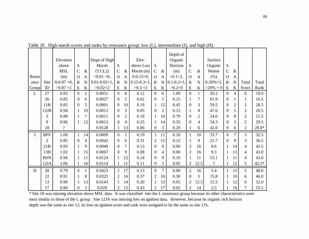
89
Table 20. High marsh scores and ranks by resistance group: low (L), intermediate (I), and high (H).
Resistance
GroupSite ID
Elevation above MSL (m)
0-0.87 =0, >0.87 =1
SCORE
RANK
Slope of High Marsh
(T1:L2) <0.01 =0,
0.01-0.02=1, >0.02=2
SCORE
RANK
Elev. above Low Marsh (m) 0-0.15=0,
0.15-0.3=1, >0.3 =2
SCORE
RANK
Depth of Organic Horizon
(m) <0.1=2,
0.1-0.2=1, >0.2=0
SCORE
RANK
Surface Organic Matter
(%) 0-20%=1, >20% = 0
SCORE
RANK
Total Score
Total Rank
L 27 0.83 0 2 0.0051 0 8 0.12 0 6 1.00 0 1 50.2 0 4 0 18.026 0.85 0 6 0.0027 0 5 0.02 0 1 0.15 1 7 61.9 0 1 1 16.5
11B 0.85 0 5 0.0091 0 10 0.19 1 12 0.45 0 3 59.5 0 2 1 28.512JB 0.94 1 10 0.0012 0 3 0.05 0 2 0.15 1 8 47.6 0 5 2 20.5
3 0.88 1 7 0.0011 0 2 0.18 1 10 0.79 0 2 24.6 0 8 2 21.59 0.96 1 12 0.0013 0 4 0.25 1 14 0.35 0 4 54.3 0 3 2 29.518 ? 0.0128 1 13 0.06 0 3 0.20 1 6 42.0 0 6 2 28.0*
I BFF 1.00 1 14 0.0009 0 1 0.19 1 11 0.10 1 10 33.7 0 7 3 32.52 0.85 0 4 0.0042 0 6 0.31 2 15 0.12 1 9 21.7 0 9 3 36.5
21B 0.93 1 9 0.0049 0 7 0.13 0 8 0.00 2 16 8.6 1 14 4 42.513H 1.02 1 15 0.0067 0 9 0.08 0 4 0.00 2 16 9.3 1 13 4 43.0BSN 0.94 1 11 0.0124 1 12 0.14 0 9 0.10 1 11 15.1 1 11 4 43.012JA 1.06 1 16 0.0114 1 11 0.11 0 5 0.05 2 12.5 ? 1 12 5 42.5*
H 28 0.79 0 1 0.0423 2 17 0.13 0 7 0.00 2 16 5.4 1 15 5 48.022 0.91 1 8 0.0325 2 16 0.37 2 16 0.30 0 5 15.8 1 10 6 46.013 0.99 1 13 0.0143 1 14 0.20 1 13 0.05 2 12.5 12.2 1 12 6 52.017 0.84 0 3 0.029 2 15 0.43 2 17 0.02 2 14 2.5 1 16 7 55.5
* Site 18 was missing elevation above MSL data. It was classified into the L resistance group because its other characteristics weremost similar to those of the L group. Site 12JA was missing loss on ignition data. However, because its organic rich horizon depth was the same as site 13, its loss on ignition score and rank were assigned to be the same as site 13's.

90
Regression factor score 1
2.52.01.51.0.50.0-.5-1.0-1.5
Re
gre
ssio
n fa
ctor
sco
re 2
3
2
1
0
-1
-2
Figure 27. Ordination plot of high marsh sites using principal components analysis.Ordination represents similarity of sites based on the five variables (elevation aboveadjacent zone, high marsh slope, depth of organic rich horizon, percent organic matter,elevation above MSL) used to classify the high marsh sites into resistance groups. Pointsare labeled with their corresponding site number and resistance groups are outlined. Site13 was the only site not grouped with its predefined resistance group.
Low
High
Intermediate
13
2
BSN
21B
13H
12JA
BFF
22 28 17
12JB
269
27
11B
3

91
467N =
Group
HIL
Ele
vato
n di
ffere
nce
(m)
.5
.4
.3
.2
.1
0.0
467N =
Group
HIL
Slo
pe
.05
.04
.03
.02
.01
0.00
-.01
Figure 28. Variables (A) elevation of high marsh above low marsh, (B) slope of highmarsh, (C) depth of organic rich zone from soil surface, (D) percent organic matter (0-10cm), and (E) elevation of high marsh above MSL, used to classify high marsh sites intothree resistance groups: low (L), intermediate (I), and high (H). Boxplot components aredescribed in Figure 17.
(A)
(B)
p = 0.1
p = 0.01

92
Figure 28. Continued.
467N =
Group
HIL
Org
ani
c ho
rizo
n de
pth
(cm
)
0
-20
-40
-60
-80
-100
-120
467N =
Group
HIL
Org
ani
c m
atte
r (%
) 70
60
50
40
30
20
10
0
3
466N =
Group
HIL
Ele
vatio
n (m
)
1.1
1.0
.9
.8
.7
(C)
(D)
(E)
p = 0.007
p = 0.003
p = 0.2

93
and I and H sites were basically similar in elevation (Figure 28E). L sites had the thickest
O horizons (Figure 28C), and the highest percent organic matter in their soil surface
(Figure 28D). I and H sites were similar in terms of organic matter characteristics; they
both had very thin O horizons and little organic matter in their soil surface.
Initially, distance to closest tidal source from the seaward side of the zone was
used in the classification procedure for these sites. However, analysis revealed there was
considerable overlap between the three resistance groups for both zones classified (forest
and high marsh) and for transition sites (Figure 29). Therefore, it was removed from the
classification procedure.
4.4 Resistance Group Comparison
Two physical components of vegetation structure varied by forest resistance
groups, but not significantly at the 0.05 level (Figure 30). Vegetated ground cover and
shrub density were inversely related (r = -0.75, p = 0.002). Forest sites with the highest
resistance had the lowest shrub densities and the most herbaceous cover, whereas forests
with the lowest resistance had the highest shrub densities and least herbaceous cover.
Tree density, basal area and canopy cover did not differ among the three resistance
groups.
Ground cover species richness did not vary by resistance group, but percent
vegetated ground cover decreased with decreasing resistance (Table 21). Woody species

94
487N =
Group
HIL
Dis
tanc
e (
m)
800
600
400
200
0
288N =
Group
HIL
Dis
tanc
e (m
)
800
600
400
200
0
467N =
Group
HIL
Dis
tanc
e (
m)
800
600
400
200
0
Figure 29. Boxplots showing distance from the nearest tidal source for the (A) forest, (B)transition, and (C) high marsh grouped by resistance groups: low (L), intermediate (I),high (H). Transition sites are grouped according to their forest’s resistance. Boxplotcomponents are described in Figure 17.
(B) Transition
(C) High marsh
(A) Forest p = 1.0
p = 0.7
p = 0.9

95
356N =
Group
HIL
He
rba
ceou
s co
ver
(%) 70
60
50
40
30
20
10
0
356N =
Group
HIL
Shr
ubs
(no.
/ha
)
4,000
3,000
2,000
1,000
0
Figure 30. Boxplots showing physical vegetation structure components for the threeforest resistance groups: low (L), intermediate (I), and high (H). Boxplot components aredescribed in Figure 17.
p = 0.06
p = 0.3

96
Figure 30. Continued.
356N =
Group
HIL
Tre
e de
nsity
(no
./ha
) 3,000
2,000
1,000
0
13
356N =
Group
HIL
Bas
al a
rea
(m^2
/ha
) 40
30
20
10
0
22
13
356N =
Group
HIL
21
13
Tre
e c
ano
py
cove
r (%
)
90
80
70
60
50
40
30
20
p = 0.9
p = 1.0
p = 1.0

97
Table 21. Relative % ground cover (0-1m) and woody species IV's for forest resistance groups: low (L), intermediate (I), and high (H). Relative cover wascalculated same as Table 10 and IV's were calculated same as Table 11. Values <1 are not reported.
Ground Cover (%) Importance ValueCover Type or Species L I H L I H
n= 18 15 9 6 5 3
Myrica cerifera 6 6 20 6 8Juniperus virginiana 5 4 24 23 12Pinus taeda 3 2 38 33 23Prunus serotina 2 6 1Nyssa sylvatica 7 3Baccharis halimifolia 2Ilex opaca 6 3Celtis occidentalis 19 32Liquidambar styraciflua 2 4 8Aralia spinosa 2 5Lirodendron tulipifera 5Magnolia virginiana 1Pinus serotina 1Persea borbonia 2Panicum virgatum 2unidentified gramminoid 5Rhus radicans 1 7 5Iva frutescens 1Limonium carolinium 2Atriplex patula 1Bignonia capreolata 4 3Asclepias incarnata 4Smilax bona-nox 10Erechtites hieracifolia 9Bare ground 4Crab burrow 7Woody debris 15 14Litter 59 57 52Wrack 3Vegetated Total 19 29 41Unvegetated Total 81 71 55Hardwood Total 9 37 58Grand Total 100 100 100 92 100 100

98
richness was slightly higher for H forest sites and hardwood species importance increased
with increasing resistance. Hardwood species IVs were 9 for L sites, 35 for I sites, and 58
for H sites (Table 21). M. cerifera and P. taeda decreased in importance with increasing
resistance, and C. occidentalis increased in importance with increasing resistance (Table
21). L sites were dominated by P. taeda, M. cerifera, and J. virginiana. I sites were
dominated by P. taeda and J. virginiana with M. cerifera and C. occidentalis next in
importance. H sites were dominated by P. taeda and C. occidentalis but also had a strong
mix of hardwoods and J. virginiana. There were no significant differences between the
three groups for dead tree or stump densities; however, the sites with the highest densities
for both components were in the L group (Figure 31).
The L forest group had significantly higher salinities (p = 0.038) compared with
the I and H groups, and significantly higher soil organic matter (p = 0.01) compared with
the H group (Figure 32). Although a significant difference was not present, depth of the
organic rich horizon was generally deeper for L sites (Figure 32).
All L forest sites, 80 % of I forest sites, and 50 % of H forest sites had transitionzones between their forest and marsh. I forest-marsh transitions occurred at the highest
elevations and H transitions occurred at the lowest elevations, where present (Figure 33).L transition sites had a wide range in elevation above MSL. There were no significant
differences between the three groups in terms of transition zone elevation above adjacentseaward zone. H transitions, where present, had much steeper slopes compared with theother two groups (p = 0.03), and were extremely narrow in width (i.e.<6 m). Transitions

99
356N =
Group
HIL
Dea
d tr
ee
den
sity
(no
./ha
)
400
300
200
100
0
356N =
Group
HIL
Stu
mps
(no
./ha
)
1,600
1,400
1,200
1,000
800
600
400
2000
12JB
Figure 31. Boxplots showing dead vegetation components for forest resistance groups:low (L), intermediate (I), and high (H). Boxplot components are described in Figure 17.
p = 0.3
p = 0.4
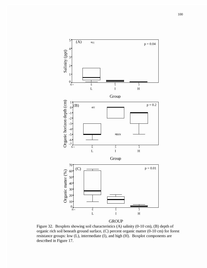
100
356N =
Group
HIL
Sa
linity
(p
pt)
5
4
3
2
1
0
11
356N =
Group
HIL
BSN
11
Org
ani
c ho
rizo
n de
pth
(cm
)
1
0
-1
-2
-3
-4
-5
-6-7
356N =
GROUP
HIL
Org
ani
c m
atte
r (%
) 70
60
50
40
30
20
10
0
Figure 32. Boxplots showing soil characteristics (A) salinity (0-10 cm), (B) depth oforganic rich soil beneath ground surface, (C) percent organic matter (0-10 cm) for forestresistance groups: low (L), intermediate (I), and high (H). Boxplot components aredescribed in Figure 17.
(A)
(B)
(C)
p = 0.04
p = 0.2
p = 0.01

101
278N =
Group
HIL
Ele
vatio
n (m
)
1.4
1.3
1.2
1.1
1.0
.9
.8
288N =
Group
HIL
Ele
vatio
n d
iffe
renc
e (
m)
.8
.6
.4
.2
0.0
-.2
288N =
Group
HIL
Slo
pe
12T
.08
.06
.04
.02
0.00
288N =
Group
HIL
Zone
wid
th (
m)
70
60
50
40
30
20
10
012T
22
Figure 33. Physical characteristics of transition sites grouped by their forest resistance groups: low (L), intermediate (I), andhigh (H). The graph displaying elevation difference refers to the elevation difference between the average elevation of thetransition zone and the average elevation of the high marsh or L2 where the high marsh is absent. Boxplot components aredescribed in Figure 17.
p = 0.2 p = 0.6
p = 0.1
p = 0.03

102
forming seaward of L and I forests varied in width from very narrow (< 6m) to very wide
(>50 m).
Physical components of the vegetation structure showed no significant differences
between the three transition groups (Figure 34). There were a few more trees in the L
transitions and subsequently more basal area and canopy cover, compared with those
transitions forming seaward of I and H forests. Tree canopy cover was present in some
sites lacking trees due to shading from trees in the adjacent forest zone. Percent
herbaceous cover did not correlate with canopy cover, tree density, or shrub density in the
transition zone.
Transition zones forming seaward of L forests differed from the others in terms of
species composition (Table 22). L transitions had the lowest S. patens cover, and the
highest percent cover of less salt tolerant species (19 %) compared with the other
transition groups (I, 9 %; H,13 %). Furthermore, L transitions had the lowest vegetated
to unvegetated ground cover ratio, and the most wrack. I forest transitions were most
different from L transitions. I sites had the lowest cover of less salt tolerant species and
the highest vegetated to unvegetated ground cover ratio. H forest transitions had a
combination of both I and L transition characteristics. For both woody species IVs and
ground cover composition, L and I transitions were most different, and H transitions
showed a combination of the two extremes. L forest transition sites were dominated by
species that were fairly salt intolerant (IV = 69). More notably, L transitions almost
always lacked or had very little of the shrub I. frutescens which is often characteristic of
transition zones. Only one L transition site, 21B, was dominated by I. frutescens and this

103
288N =
Group
HIL
He
rbac
eous
cov
er
(%)
80
60
40
20
0
288N =
Group
HIL
Shr
ubs
(no.
/ha
)
5,000
4,000
3,000
2,000
1,000
0
Figure 34. Boxplots showing vegetation structure components for transition sites groupedby their forest resistance groups: low (L), intermediate (I), and high (H). Boxplotcomponents are described in Figure 17.
p = 0.2
p = 0.2

104
Figure 34. Continued.
288N =
Group
HIL
Tre
e de
nsity
(no
./ha
) 600
500
400
300
200
100
0
BSN
288N =
Group
HIL
Ba
sal a
rea
(m
^2/h
a) 10
8
6
4
2
0BSN
288N =
Group
HIL
Ca
nop
y co
ver
(%) 50
40
30
20
10
0
Table 22. Relative percent ground cover (0-1m) and woody species IVs for transition
p = 0.2
p = 0.2
p = 0.3

105
sites grouped by forest resistance groups: low (L), intermediate (I), and high (H).Relative cover was calculated same as Table 10 and IVs were calculated same asTable 11. Values <1% are not reported. Less salt tolerant species (LST) areindicated with an *.
Ground Cover (%) Importance ValueCover Type or Species L I H L I H
n= 39 48 6 13 16 2
Pinus taeda* 2 1 11 2Juniperus virginiana* 1 31 7 4Myrica cerifera* 5 10 27 21Iva frutescens 10 22 12 21 73 54Baccharis halimifolia 5 10 19 21Typha sp.* 2unidentified graminoid* 1 1Spartina patens 14 29 29Distichlis spicata 7 12 2Panicum virgatum* 7 5 2Setaria viridis* 1 1Juncus roemerianus 7 5Spartina alterniflora 1 7Juncus gerardi 7Limonium carolinium 1Asclepias incarnata* 1Stump 1Dead tree 1 1Dead shrub 2 1Woody debris 4 1Wrack 11 1Litter 16 5 19Bare ground 8 4 14Pothole 2Vegetated Total 58 85 76Unvegetated Total 42 15 33LST species (*) Total 19 9 13 69 9 25Grand Total 100 100 100 100 100 100

106
site was unusual in that it was the only L forest site with nonhydric soils. Transitions
forming seaward of L forests were dominated by M. cerifera and J. virginiana in the
shrub stratum, but also had P. taeda and B. halimifolia. Transitions forming seaward of I
forests were all dominated by I. frutescens. Most I transitions also had a prevalence of B.
halimifolia and/or J. virginiana. Species composition was more variable in H transitions;
I. frutescens dominated one of the H forest transition sites while B. halimifolia and M.
cerifera dominated the other. However, because the sample size for H transitions is so
low (n = 2) it is hard to draw conclusions about this group.
Dead shrub densities had a similar pattern for both size classes (<1 m and >1 m).
L and H transitions had no dead shrubs and I transitions ranged between 0-400 stems/ha
for both size classes with exception for one outlier (Figure 35). Dead shrub densities of
both size classes were inversely related to salinity (shrubs <1 m r = -0.68, p = 0.003;
shrubs >1 m r = -0.67, p = 0.004). In general, dead tree density did not differ between the
groups, although site 12JA, a small island, had an unusually high dead tree density 1,400
stems/ha). Stump density did not significantly differ between the three transition groups.
Neither dead tree nor stump density were correlated with salinity.
Overall, soil characteristics did not significantly vary between the three transition
groups (Figure 36). However, forest-marsh transitions with the highest salinities or
deepest O horizons occurred next to I forests.
High marsh sites differed in several soil and physical factors, not used in the
classification scheme, by group. Salinity decreased with increasing resistance to regular
brackish water flooding and drainage potential (Figure 37). Most L high marsh sites

107
288N =
Group
HIL
De
ad
shr
ubs
<1
m (
no./
ha)
500
400
300
200
100
0
288N =
Group
HIL
Dea
d sh
rubs
>1m
(no
./ha
)
800
600
400
200
0
22
10
288N =
Group
HIL
De
ad
tre
e d
ens
ity (
no./
ha)
1,600
1,400
1,200
1,000
800
600
400
2000
12JA
288N =
Group
HIL
Stu
mp
s (n
o./
ha)
800
600
400
200
0
Figure 35. Dead vegetation components for transition sites grouped by their forest resistance groups (low (L), intermediate (I),and high (H). Boxplot components are described in Figure 17.
p = 0.002 p = 0.005
p = 0.6 p = 0.7

108
278N =
Group
HIL
Sa
linity
(p
pt)
10
8
6
4
2
0
12JB
288N =
Group
HIL
Org
ani
c ho
rizo
n d
ep
th (
cm)
0
-10
-20
-30
278N =
Group
HIL
Org
ani
c m
atte
r (%
) 50
40
30
20
10
0
2
Figure 36. Boxplots showing soil characteristics (A) soil salinity (0-10 cm), (B) depth oforganic rich horizon from ground surface, and (C) percent organic matter (0-10 cm) oftransition sites grouped by their forest resistance groups: low (L), intermediate (I), andhigh (H). Boxplot components are described in Figure 17.
p = 0.6
p = 1.0
p = 0.9
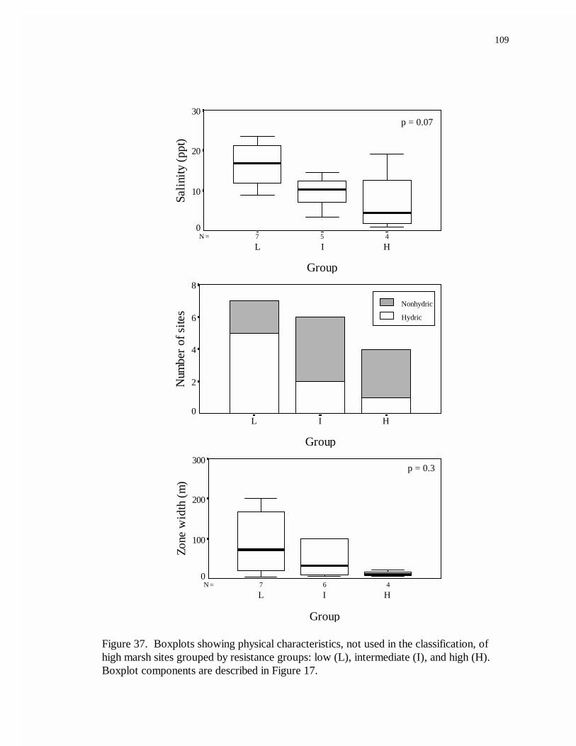
109
457N =
Group
HIL
Sa
linity
(pp
t)
30
20
10
0
Group
HIL
Num
ber
of s
ites
8
6
4
2
0
467N =
Group
HIL
Zone
wid
th (
m)
300
200
100
0
Figure 37. Boxplots showing physical characteristics, not used in the classification, ofhigh marsh sites grouped by resistance groups: low (L), intermediate (I), and high (H).Boxplot components are described in Figure 17.
p = 0.07
p = 0.3
Nonhydric
Hydric

110
formed seaward of hydric soils, whereas most I and H sites formed seaward of nonhydric
soils. L and I sites generally had the widest high marsh zones whereas H sites had very
narrow zone widths.
There were no significant trends between the three high marsh resistance groups in
physical components of their vegetation structure (Figure 38). However, L high marsh
sites usually lacked or had very few shrubs. Shrub density was inversely related to salinity
(r = -0.51, p = 0.045) and percent herbaceous cover (r = -0.65, p = 0.005). The ratio of
vegetated to unvegetated ground cover was similar for the three high marsh resistance
groups (Table 23). I high marsh sites had a much lower percent cover of Spartina patens
than the other two groups and had the most J. roemarianus and D. spicata cover. Iva
frutescens had the lowest percent ground cover in L high marsh sites. Iva frutescens was
the most important woody plant for all high marsh groups. B. halimifolia was also
present in all groups.
L and H high marsh groups were similar in that they both commonly lacked dead
short shrubs (<1 m), dead trees, and stumps (Figure 39). A few sites in the L group had
dead tall shrubs (>1 m) but H sites had none. I high marsh sites had the most dead short
shrubs <1 m, dead trees, and stumps. Site 12JA, the small island, had a high dead tall
shrub (>1 m) density.
4.5 Resistance Group Map and Field Indicators
Two L forests lacked high marsh, four had L high marsh states, and three had Ihigh marsh states (Table 24). Both sites (10,11) lacking high marsh occurred on wetland

111
467N =
Group
HIL
He
rba
ceo
us c
ove
r (%
)
120
110
100
90
80
70
60
50
467N =
Group
HIL
Shr
ubs
(no.
/ha
)
3,000
2,000
1,000
0
27
Figure 38. Boxplots showing physical vegetation structure components for high marshresistance groups: low (L), intermediate (I), and high (H). Boxplot components aredescribed in Figure 17.
p = 0.5
p = 0.4

112
Table 23. Relative percent ground cover (0-1m) and woody species IVs for highmarsh sites grouped by their resistance groups: low (L), intermediate (I), and high (H).Relative cover was calculated same as Table 10 and IVs were calculated same asTable 11. Values <1% are not reported.
Ground Cover (%) Importance Value
Cover Type or Species L I H L I H
n= 51 36 15 17 12 5
Iva frutescens 2 7 9 30 50 47Baccharis halimifolia 1 2 3 3Spartina patens 47 21 53Distichlis spicata 23 38 21Limonium carolinium 1 1 2Juncus roemerianus 7 19Spartina alterniflora 4 1Juncus gerardi 7 3Setaria viridis 3Atriplex patula 1Borrichia frutescens 2Dead shrub 1Pothole 4 3Bare ground 2 6 3Wrack 3 2 2Vegetated Total 91 88 95Unvegetated Total 9 12 5Grand Total 100 100 100 32 53 50

113
467N =
Group
HIL
De
ad
shr
ubs
<1
m (
no./
ha)
1,200
1,000
800
600
400
200
0
18
467N =
Group
HIL
De
ad
shr
ubs
>1
m (
no./
ha)
700
600
500
400
300
200
100
0
12JA
27
467N =
Group
HIL
Dea
d tr
ee
dens
ity (
no./
ha)
400
300
200
100
0
467N =
Group
HIL
Stu
mp
s (n
o./
ha)
800
600
400
200
0
Figure 39. Boxplots showing dead vegetation components for high marsh resistance groups: low (L), intermediate (I), and high(H). Boxplot components are described in Figure 17.
p = 0.2 p = 0.3
p = 0.03 p = 0.01

114
Table 24. Field sites listed with their respective zones and zone widths. Forest and highmarsh zones are listed by resistance group (low (L), intermediate (I), high (H)) or absent(-), and ground water seep zones are listed as present (+) or absent (-).
Site
ForestResistance
Group
TransitionZone Width
(m)
High MarshResistance
Group
High MarshZone Width
(m)Ground-
Water Seep10 L 55 - 0 -11 L 20 - 0 -3 L 4 L 176 -9 L 4 L 157 -
12JB L 42 L 202 -11B L 8 L 72 -
2 L 7 I 100 -BFF L 30 I 99 -21B L 12 I 33 -
12T I 6 - 0 -21 I 22 - 0 -18 I 18 L 4 -
12JA I 26 I 6 -BSN I 21 I 8 -13H I 18 I 32 -13 I 20 H 13.5 -22 I 60 H 8 -17 I 0 H 20 -28 I 0 H 6 -
5 H 0 - 0 +8 H 3 - 0 -26 H 6 L 6 -27 H 0 L 33 +

115
islands or necks (Table 25). Regardless of resistance category to which a given high
marsh belonged, when occurring next to L forests most were very wide (i.e. >70 m). The
only exception was site 21B which was unique to the L forest group because its forest soil
type was nonhydric (Table 25). Two I forest sites lacked high marsh, one had a high
marsh in the low resistance category, three had I high marsh states, and four had H high
marsh states. I forests tended to have high marsh widths that ranged from narrow (4 m)
to somewhat wide (30 m). Two H forest sites lacked high marsh and the other two had
low resistance high marsh states that varied in width (6 m and 33 m). One H forest site
with high marsh and one without high marsh had groundwater seeps between forest and
marsh. Both sites with a groundwater seep lacked a transition zone; the two without
groundwater seeps had transitions but both very narrow (3 m and 6 m) (Table 24).
It was possible to identify all L forest sites using soil survey and USGS
topographic maps by subdividing L forests into four subgroups (La, Lb, Lc, Ld) (Figure
40). La sites occurred on island or neck landforms with hydric forest soils (Table 25). Lb
sites occurred on interfluve landforms that had hydric forest soils for extensive widths (i.e.
>50 m) and/or the hydric Magotha (MaA) series (i.e. the soil series that high marsh and
transition occurred on) for fairly extensive widths (i.e. >50 m). Widths were measured
perpendicular to the estuarine boundary and scarp. Lc sites occurred on valley landforms
and had hydric forest soils. Ld sites occurred on interfluve landforms with nonhydric forest
soils and some MaA. The key feature of the Ld site was that it had a very wide (700 m)
distance between the 1.5-3.0 m contours.
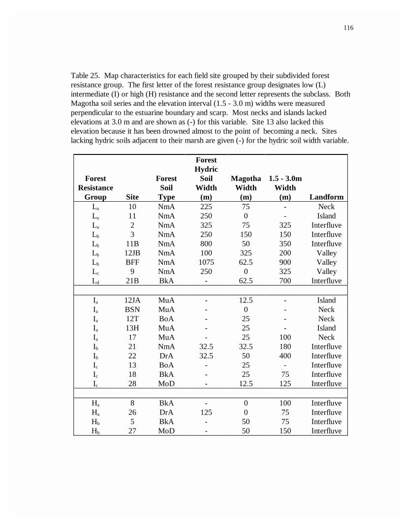
116
Table 25. Map characteristics for each field site grouped by their subdivided forestresistance group. The first letter of the forest resistance group designates low (L)intermediate (I) or high (H) resistance and the second letter represents the subclass. BothMagotha soil series and the elevation interval (1.5 - 3.0 m) widths were measuredperpendicular to the estuarine boundary and scarp. Most necks and islands lackedelevations at 3.0 m and are shown as (-) for this variable. Site 13 also lacked thiselevation because it has been drowned almost to the point of becoming a neck. Siteslacking hydric soils adjacent to their marsh are given (-) for the hydric soil width variable.
ForestResistance
Group Site
ForestSoil
Type
ForestHydric
SoilWidth
(m)
MagothaWidth
(m)
1.5 - 3.0mWidth
(m) LandformLa 10 NmA 225 75 - NeckLa 11 NmA 250 0 - IslandLa 2 NmA 325 75 325 InterfluveLb 3 NmA 250 150 150 InterfluveLb 11B NmA 800 50 350 InterfluveLb 12JB NmA 100 325 200 ValleyLb BFF NmA 1075 62.5 900 ValleyLc 9 NmA 250 0 325 ValleyLd 21B BkA - 62.5 700 Interfluve
Ia 12JA MuA - 12.5 - IslandIa BSN MuA - 0 - NeckIa 12T BoA - 25 - NeckIa 13H MuA - 25 - IslandIa 17 MuA - 25 100 NeckIb 21 NmA 32.5 32.5 180 InterfluveIb 22 DrA 32.5 50 400 InterfluveIc 13 BoA - 25 - InterfluveIc 18 BkA - 25 75 InterfluveIc 28 MoD - 12.5 125 Interfluve
Ha 8 BkA - 0 100 InterfluveHa 26 DrA 125 0 75 InterfluveHb 5 BkA - 50 75 InterfluveHb 27 MoD - 50 150 Interfluve

117
Highmarsh
absent &very close
to tidalcreek
Very flat slopes,wide high marsh zone &
transition zone dominatedby less salt tolerant
species
LOW INTERMEDIATE
Figure 40. Map and field indicators for subclasses (a, b, c, d) of forest resistance groups (low, intermediate, high). Ic and Hb
sites are not distinguishable from each other on topographic and soil survey maps. MaA refers to Magotha soil series, a hydricsoil typically found in high marsh and transition zones.
HIGH
La Lb Lc Ld Ia Ib Ic Ha Hb
Wetlandisland
or neck
Interfluvelandform
with foresthydric soils>50m wide
& MaA soils
Valleylandform
with hydricforest soils
Nonhydricforest soilswith MaA
soils & longdistancebetween
1.5 - 3.0 m
Uplandisland
or neck
Interfluvelandformw/ hydric
forest soils<50m wide
& MaAsoils <50m
wide
Uplandforest
soils w/MaAsoils
Interfluvelandformlacking
MaA soils
Uplandforest
soils w/MaAsoils
MAP
INDICATORS
FIELD
INDICATORS
Transition slope< 0.01
Forest elevationabove seaward zone
< 0.50 m
Transitionzone
dominatedby Iva;
narrow highmarsh maybe present
and
orNo
transitionzone andnarrow
high marsh
Forest elevation aboveseaward zone
>0.50 m
and
Verynarrow
highmarsh and
ortransition
zone
Ground-waterseep
or
or

I forest sites were also subdivided into three subgroups (Ia, Ib, Ic) using soil survey
and USGS topographic maps. Ia sites occurred on island or neck landforms with
nonhydric forest soils (Table 25). Ib sites occurred on interfluve landforms with hydric
forest soils that were not very extensive in width (i.e. <50 m) and MaA that was not very
extensive in width (i.e. <50 m). The three Ic sites had forests with nonhydric soils and
MaA present, but distances between the 1.5-3.0 m contours were only moderate (75 m
and 125 m) compared to the Ld site (700 m).
H forest sites were subdivided into two subgroups (Ha, Hb) using USGS
topographic and soil survey maps. Ha sites occurred on interfluve landforms that lacked
MaA soils (Table 25). Forest soil type was not an indicator of Ha sites. Hb sites were not
distinguishable from Ic sites on maps. They both had nonhyric forest soils, MaA soils, and
had moderately wide distances (75 m and 150 m) between their 1.5-3.0 m contour lines.
In addition to map indicators, field indicators were also identified for the forest
resistance groups (Figure 40). La sites lacked a high marsh zone and their forests occurred
very close (within 55 m) to a tidal creek. However, it is possible that wetland necks
occurring along the Machipongo River valley may look more similar to Lb or Lc groups in
the field because they have wide expanses of MaA soils located along them. Lb and Lc
groups had very gradual slopes between their forest and marsh, very wide high marsh
zones (>70 m), and had transition zones dominated by less salt tolerant species (M.
cerifera, J. virginiana, P. taeda). The Ld forest site appeared similar to I forest sites in the
field. These sites (Ld, Ia, Ib, Ic) had transition zones dominated by I. frutescens and had
fairly narrow (<35 m) to nonexistent high marsh zones.

cxix
It may be difficult to distinguish Ha sites from I sites in the field without elevation
measurements. Ha sites had very narrow transition zones that were dominated by I.
frutescens, or B. halimifolia and M. cerifera. The key difference between Ha and I forests
is that the elevation difference between Ha forests and their adjacent seaward zone was at
least 0.57 m whereas it was always <0.4 m for I sites. Ha sites were easily distinguished
from the Ld site in the field because the Ld site had a very gradual transition slope (0.007)
compared to Ha sites (0.07 and 0.025). Hb sites had very steep slopes between marsh and
forest, lacked a transition zone, and were in the only subgroup with groundwater seeps.
The seeps were vegetated with Phragmites australis or Scirpus sp. Although I only
sampled two Hb sites, I observed many steep transitions vegetated with P. australis. P.
australis also occurred in places where freshwater creeks entered marshes, but these
locations were distinguished from Hb sites because they had much more gradual slopes
than the Hb sites. It is possible that Ha sites may also support groundwater seeps;
however, I did not sample any that did.
The map indicators I identified were useful for characterizing the degree of
resistance for 149 forest sites using USGS topographic and soil survey maps. Most of the
forest to marsh coastline occurred along upland necks and islands (Ia); Ld and Ib forest
sites were rare; and there were approximately the same number of La, Lb, Lc, Ic/Hb, and Ha
forest sites (Figure 41). The central region had the largest number of forest sites adjacent
to marshes, and had forests within all subgroups; however most of these had either low or

cxx
Figure 41. Number and percent of map sites within each forest resistance subgroup. Sites are comprised of all forests adjacent to marshes along 60 map transects and 7 additional field sites.
Figure 42. Number of sites within each forest resistance group by geographic region. Sites are comprised of all forests adjacent to marshes along 60 map transects and 7 additional field sites. Ic/Hb sites were split evenly between the intermediate and high resistance groups
0
20
40
60
80
100
120
South Central North
Region
Num
ber
of s
ites
High
Intermediate
Low
0
5
10
15
20
25
30
35
40
45
50
La Lb Lc Ld Ia Ib Ic/Hb Ha
Resistance subgroup
Num
ber
of s
ites
14 %
10 % 10 %
1 %
34 %
3 %
14 % 14 %
La Lb Lc Ld Ia Ib Ic/Hb Ha

cxxi
intermediate resistance (Figures 42 and 43). Half of the coastal forests in the south region
had low resistance and all of these were in the Lb subgroup (Figures 42 and 43). Ic and Hb
sites made up the next largest proportion of the south region. Most of the coastal forests
in the north region had high resistance (Figures 42 and 43).

cxxii
Figure 43. Pie charts showing percent of map sites in each forest resistance subgroup by geographic region. Sites are comprised of all forests adjacent to marshes along 60 map transects and 7 additional field sites.
South Region
Lb 50%
Ib 13%
Ic /Hb
31%
Ha 6%
Central RegionLa 19%
Lb 5%
Lc 14%
Ld 1%Ia 45%
Ib 3%
Ic /Hb 8%
Ha 6%
North Region Lb 9%
Ib 5%
Ic /Hb
32%
Ha 55%

cxxiii

cxxiv
5. DISCUSSION
The objective of this study was to characterize the mainland fringe of the VCR
Megasite in terms of patterns where ecosystem state change is most likely to occur.
Pattern characterization took place at two scales: a broad scale (10’s of kilometers) that
separated the Megasite into three geographic regions, and a smaller scale (10’s of meters)
that was more relevant to predicting state change. Patterns will be used to make
predictions about the relative rate of state change within the different spatial scales.
In order to discern the broad pattern, soil types and elevation intervals were
quantified for the three geographic regions using maps. Small scale patterns were
established through a four step process. First, the four ecosystem states were
characterized by gathering map and field data on their soils, vegetation patterns, and
elevations. Forest and high marsh states were then classified, based on physical attributes,
into three resistance groups according to their level of resistance (low, intermediate, high)
to state change. Attributes of the three resistance groups, for each ecosystem state, were
compared to determine if they were in different stages of a state change. Finally, a rapid
assessment procedure is developed that uses only a few map and field indicators to identify
forest resistance groups.
5.1 Outlook for Three Geographic Regions of Megasite
The central region has the most land area available for forest conversion to marshbecause it has the most area at lower elevations (below 1.5 m and between 1.5 and 3.0 m),and the most area of hydric soils (Figure 44). Elevations <1.5 m are most likely to be

cxxv
0-1.5 m1.5 - 3.0 m
3.0 - 7.6 mCENTRALREGION
Figure 44. Cross section of terrace plain through the three geographic regions.Elevation intervals represent the average of each region and are proportionate amongregions.
NORTHREGION
0-1.5 m
1.5 - 3.0 m
3.0 - 7.6 m
SOUTHREGION
0-1.5 m
1.5 - 3.0 m
3.0 - 7.6 m
cxxvi
affected by rising sea level within the next 80 years, based on a rise of 5 mm/year (IPCC
best estimate). At this rate, in 80 years sea level should be 0.4 m higher than present, and
transition zone (currently elevated at 1.1 m) would have shifted 0.4 m upslope to replace
forests located <1.5 m in elevation. Elevations between 1.5 and 3.0 m are unlikely to
experience significant encroachment over the next 80 years, because they would still be
situated above 1.5 m. Instead, they should become the new platform for marsh
transgression in the following century. Coastal forests occurring on hydric soils are more
susceptible to state change than those on upland soils because hydric soils are poorly
drained. Poor drainage increases the duration of salts and reduced soil conditions, thus
prolonging the time that vegetation is exposed to these stressors. Prolonged exposure to
stressors causes forest vegetation die-back which leads to a more open canopy and less
ground shading. These conditions encourage marsh species invasion and hence state
change.
The north and south regions have very similar land areas of low elevations and
transition soils, and have much less area available for forest conversion to marsh than does
the central region (Figure 44). Although the south region has little area (389 ha) available
for forest conversion to marsh, 50 % of its coastline has low resistance to state change,
suggesting that the area available for conversion will change state fairly rapidly. In
contrast, 91 % of the coastal forests in the north region, which also has little area (299 ha)
available for forest conversion to marsh, has intermediate to high resistance to state
change, and therefore will not change state as rapidly as the south region. Finally, 39 % of
the coastal forests in the central region, which has the most land area (5,254 ha) available

cxxvii
for forest conversion to marsh, has low resistance to state change and will likely undergo a
transformation in the next 50 - 100 years. Based on these results, the north and south
regions are prone to experience a net loss in marshes over the next 100 years while the
central region is likely to experience a net loss in forests.
5.2 Ecosystem State Characteristics
In general, four ecosystem attributes (species richness, physical vegetation
structural complexity, soil organic matter, soil salinity) changed with each successive
ecosystem state change (Figure 45). The degree and direction of each attribute change
depends on the specific state change under consideration, and are believed to result from
differential flooding regimes among the states. Consequently, each state had a unique
suite of characteristics.
Coastal forests were dominated by various hardwood and coniferous trees, had an
average basal area of 17 m2/ha, and a full tree canopy cover. There were few shrubs, little
herbaceous ground cover, and rare occurrence of halophytic plants. Soil organic matter
and salt concentrations in the forest soils were relatively low, on average, compared with
the other states, and evidence of reduced soil conditions varied depending on soil drainage
type.
As forests become exposed to estuarine flooding for sufficient time, they are
replaced with transition zones. Transition zone attributes resemble a mixture between the

127
Increase
State
Decrease
Forest Transition High marsh
Lowmarsh
Salinity
Organicmatter
Salinity
Organic matter
Herbaceouscover Salinity
Elevation Tree density
Basal area
Canopy cover
Elevation Shrubdensity
Elevation Herbaceouscover
AbioticVariable
BioticVariable
Figure 45. Summary of changes that occur with each state change in response to rising sea level. Variables that increase with statechange are shown on top and variables that decrease or are lost with state change are shown on bottom.
Shrubdensity
Herbaceouscover
forest and high marsh, in addition to having characteristics unique to the zone. Dead trees
and tree stumps dispersed throughout the transition are evidence that it replaced what
formerly was forest. Shrubs were the dominant vegetation in the transition zone, but a
few trees and some herbaceous ground cover also contributed to cover. Trees, where
present, had little basal area, were either Pinus taeda or Juniperus virginiana, and
generally provided little canopy cover above 3 m. Transition zone shrub species were
comprised of both halophytes (Baccharis halimifolia and Iva frutescens) and glycophytes
(Myrica cerifera, J. virginiana, Pinus taeda). Transition zone herbaceous cover averaged
52 % and was composed predominately of high marsh species (Spartina patens, Distichlis
spicata, Juncus spp.), but also had some fairly salt intolerant species (Panicum virgatum
and Setaria viridis). Soils in the transition zone had slightly deeper organic rich horizons
and higher salt content than the forest, but both were generally lower than the high marsh.
Most soils in the transition zone showed signs of reduced conditions.
As the land surface becomes flooded more often by spring tides, severe storm
events, and precipitation (Stasavitch 1998), transition zone shrubs and trees die and are
replaced almost exclusively with herbaceous species, typical of the high marsh. Dead
shrubs dispersed throughout the high marsh indicate that replacement of the transition
zone has occurred. High marsh herbaceous species composition was dominated by a few
halophytes: S. patens, D. spicata, and J. roemerianus. Both soil salinity and organic
matter content and depth were much higher in the high marsh than the transition or forest,
and all high marsh soils showed signs of reduced conditions.

cxxix
As the land surface becomes flooded daily with estuarine tides, high marsh is
replaced by low marsh. Low marsh characteristics from this study do not represent the
entire low marsh state, but rather the 24-m width zone adjacent to high marsh. Low
marsh was colonized by a monospecific stand of Spartina alterniflora which covered on
average 60 % of the ground. No trees or shrubs were present in this zone but the
occurrence of tree stumps were again evidence the area once had been forest. Soil salinity
and organic matter depth were greater in the low marsh than high marsh but percent
organic matter was lower in the low marsh than high marsh. Finally, all low marsh soils
had indicators of reduced conditions.
Most ecosystem attributes measured in this study appear to be changing in the
direction projected by the Brinson et al. (1995) state change model. Attribute changes
consistent with the authors’ state change model include (1) loss of woody species and
species richness, (2) loss of vegetation vertical complexity, and (3) increase in salinity with
seaward state changes. However, results from this study differ from those proposed in the
state change model (Brinson et al. 1995) for soil organic matter dynamics. Brinson et al.
(1995) hypothesize that soil organic matter should increase with state change from forest
to high marsh and then decrease with state change from high marsh to low marsh. Results
from this study show that soil organic matter increased as forest was replaced by high
marsh. However, soil organic matter was not always lost as high marsh was replaced by
low marsh. Furthermore, individual sites (versus state averages) did not always conform
to trends found in this study or those proposed by Brinson et al. (1995). For example, not
all high marshes developed organic rich horizons. These discrepancies suggest that
cxxx
mechanisms driving state change may not be as simple or predictable as described by
Brinson et al. (1995).
5.3 Causes of State Change
Soil and vegetation characteristics altered by longer flooding regimes are due to
both abiotic and biotic influences. Flooding frequency and duration increase with each
seaward state change (Stasavitch 1998), and these hydrodynamics act to change soil
characteristics. First, increased estuarine flooding introduces a higher concentration of
salts to the soils. Also, a longer hydroperiod reduces oxygen concentrations, causes lower
soil redox potentials, and results in higher reduced Fe, Mn, and S ion concentrations
(Mohanty and Dash 1982). Soil physiochemical changes associated with longer
hydroperiods, impede organic matter decomposition, and result in increased organic-rich
stratum thickness with each seaward state change. A reduction in percent organic matter
of low marsh soils, without a similar reduction in organic matter depth, may be due to
greater mineral sedimentation rates from regular tidal flooding.
Vegetation structural complexity and species richness, also, are affected by soil
physiochemical changes. Reduced soil conditions and salt accumulation have been shown
to stress or limit production in marsh grasses (Pearcy and Ustin 1984, DeLaune et al.
1987, Koch and Mendelssohn 1989, Bertness and Ellison 1987, Bertness 1992, Broome et
al. 1995) and woody vegetation (Penfound and Hathaway 1938, Kjerfve 1979, Brinson et
al. 1985, Salinas et al. 1986, Conner et al. 1989, Young et al. 1994, Hacker and Bertness
1995, Conner et al. 1997). As these stressors increase in each seaward zone, the number

cxxxi
of species able to tolerate them decreases as indicated by decreasing species richness. This
point is made obvious by the fact that the low marsh is typically a monospecific stand of
Spartina alterniflora. Miller and Egler (1950), Eleuterius (1972), Jaworski and Tedrow
(1985), and Hmieleski (1994) have described the same trend of declining species numbers,
and hence structural complexity, with closer proximity to the sea. It is not always clear
which stressors are most controlling, and likely they act in concert to produce the distinct
vegetation zonation in these coastal wetlands (Kurz and Wagner 1957, Frey and Basan
1978).
In addition to the large role of physiochemical soil properties in plant zonation,
competition between species also plays a role (Bertness 1991). Because of height
advantages, trees are able to out-compete shrubs for light, and shrubs are able to out-
compete marsh grasses for light (Brinson et al. 1995). However, in each scenario, the
better light competitor is more sensitive to physiochemical stressors. So as trees become
stressed and die, shrubs become abundant, and as shrubs become stressed and die, grasses
become abundant. Marsh grass zonation is also a reflection of both abiotic and biotic
controls. Spartina patens is restricted to the high marsh because of physiochemical
stressors in the low marsh, whereas S. alterniflora is excluded from the high marsh state
by competition for space with high marsh species (Bertness and Ellison 1987).
5.4 Resistance Group Classification
The four variables used to classify forest resistance groups were highly
intercorrelated, raising the question of the value of the redundancy. Variables used in the

cxxxii
classification were chosen to represent a forest’s ability to resist brackish water flooding
or to drain brackish waters once flooded. For the two variables used to describe forest
elevation (elevation above MSL, elevation difference between forest and adjacent seaward
zone), redundancy was useful for both practical and conceptual reasons. In terms of
practicality, elevation difference between the forest and adjacent seaward zone data was
much easier to obtain than elevation above MSL because a permanent bench mark was not
required. I was able to obtain reliable data for all sites using this variable unlike elevation
above MSL data where I have measured values for some sites and estimated values for
others. However, elevation above MSL data was necessary because it served as a
standard for comparison between sites. Conceptually, elevation difference between forest
and adjacent seaward zone may be more representative of the elevation at which forest
will convert to transition because it takes into account individual nuances of a site that I
did not incorporate. For example, direction of forest orientation (northeast facing, west
facing, etc.), distance to tidal source, or specific site alterations may all have some
influence on the rate of forest state change but these were either not measured or were
unreliable due to inconsistent patterns.
The two variables used to describe the forest’s drainage potential (slope and soil
type) represent different scales that influence the drainage of brackish water. Soil drainage
type is likely related to the relative duration brackish water remains within soil pore
spaces. In contrast, slope defines the hydraulic gradient of the site and therefore the
direction and rate of water flow both below and above ground (Hmieleski 1994). Because
cxxxiii
slope has been shown to overcome drainage restrictions for some but not all soils (Harvey
and Odum 1990), soil drainage type was weighted less than slope.
The classification criteria appeared to be effective in separating three fairly discrete
groups with minimal overlap between resistance groups for the three numerical
classification variables. Although the groups were distinct, their scores and ranks
essentially formed a continuum from low to high. It is not clear why site 26 was grouped
closer to I sites in the ordination plot. The ordination was based on standardized scores
compared to the data set mean. It is possible that it compressed the remaining sites
because the other three H sites were much different from the mean in the two elevation
variables.
Organic matter characteristics (depth and percent) were added to elevation and
slope variables for classification of high marsh sites because organic matter is both a result
of and a control over variables affecting high marsh resistance to state change. Organic
matter accumulation results from poor drainage and therefore is an indicator of drainage
potential. However, once organic matter has accumulated it exerts control over marsh
drainage because its high water storage capacity. As a result, organic matter remains
saturated for long durations and may retain salts for longer durations than mineral soils.
Furthermore, organic matter can influence marsh elevation due to its low bulk density and
susceptibility to decomposition. Sites with deep organic horizons have a high potential for
rapid elevation decline if organic layers decompose or erode. Also, the rhizosphere, which
contains live material and is included in the organic rich horizon, loses volume when plants
die. As elevation declines, the relative rate of sea level rise increases and subsequently the

cxxxiv
relative rate of state change. For example, DeLaune et al. (1994) reported a 15 cm
elevation decline over two years from peat collapse in a Mississippi Deltaic marsh.
Unlike the three forest groups, high marsh groups were not distinctly different
from each other for all classification variables. Both elevation difference between high
marsh and low marsh and slope of high marsh, and percent organic matter and depth of
organic matter had the same grouping results. It appears that using just elevation above
MSL, high marsh slope and depth of organic matter would have resulted in the same
grouping of sites. Results suggest that having both gentle slopes and low elevations are
necessary to sustain the hydroperiod required for deep organic horizons to form. Neither
intermediate resistance high marsh sites that had gentle slopes but high elevations, nor
high resistance high marsh sites that had relatively low elevations but a steep slopes, had
deep accumulations of organic matter.
Although I was unable to identify map indicators of high marsh resistance groups,
they can be detected with minimal effort in the field. L high marsh sites can be identified
as having deep organic horizons (i.e. >20 cm) and gentle slopes; I sites have little to no
organic matter and gentle slopes, and H sites have steep slopes and no organic matter.
5.5 Stages of State Change for Resistance Groups
Low resistant forests appeared to be in a more advanced stage of state change to
transition than I or H forests. Low resistant F1 plots (F1 = seaward-most forest plot) had
vegetation and soil characteristics more similar to the transition zone than I and H forests.
cxxxv
L forests had higher shrub densities and very low hardwood importance values. In
contrast, I and H F1 plots had very few to no shrubs, and hardwoods composed a large
portion of the woody species composition. Since dead vegetation components and canopy
cover did not differ among the three forest resistance groups, it is not apparent why shrub
density is higher for L forest sites. It is possible that my measure of canopy cover was not
sensitive enough to distinguish between functionally different levels of light penetration.
Rather, leaf area index, a ratio of leaf area to ground area, may be more useful in
determining light penetration. Alternatively, higher shrub densities may reflect slower
growth rates in P. taeda and J. virginiana for L forests rather than recent invasion of new
individuals as a result of increased sunlight penetration to the forest floor. L forests had
the deepest organic rich horizons with the highest organic matter percentages; however,
because L forests were defined as those with poorer drainage potential, these results are
not surprising. Finally, higher salinities in L forest soils suggest brackish water intrusion is
either occurring more frequently or is not compensated for as quickly by flushing.
Differences between attributes of transition zones forming seaward of forest
resistance groups support the assumption that L, I, and H forests are in different stages of
state change. Compared with I and H groups, transitions occurring between L resistant
forests and marsh had characteristics more similar to forest, indicating they may have
formed more recently. In contrast, I transitions had characteristics least similar to a forest,
suggesting their forests had not undergone recent change. Similarly, Hmieleski (1994)
reported a sharp zonation between transition and forests occurring on steep slopes, and a
wider ecotone between forest and its transition occurring on gentle slopes. Vegetation

cxxxvi
and soil characteristics for transitions occurring next to H forests were more similar to I
than L transitions. However, because the H transition data set is represented by only two
sites, it may not cover the range of variation along the Megasite.
Transition zones adjacent to L forests had the most remaining trees, highest basal
area, highest canopy cover, and the lowest ratio of vegetated to unvegetated ground cover
compared with transitions adjacent to I or H forests. Also, woody species composition of
L forest transition zones was composed of glycophytes (M. cerifera, J. virginiana, P.
taeda) whereas species dominating transition sites adjacent to I and H forests were more
salt tolerant. Moreover, the fact that I transitions similar to L transitions in terms of depth
and percent of organic matter, even though they started from a forest with almost no
organic matter, may imply they have been in the transition phase longer.
Unexpectedly, width of the transition zone was not always related to resistance
group. L forests were expected to have wider transition zones than I or H forests as an
indication that more area was undergoing state change. In fact, the forest with the lowest
slope had a transition zone width of only 4 m. A possible explanation for the lack of
transition width along these gentle gradient slopes is that dead trees and shrubs were
eliminated through an episodic event such as a fire. If this occurred, then transition
replacement by high marsh likely took place at a faster rate as competition for sunlight was
eliminated. In fact, regardless of transition width, all L forest sites had very wide high
marsh zones. Any transition present today would then represent state change that has
occurred since the last fire. Young (1995) described state changes in coastal forests of
North Carolina as occurring in a punctuated stepwise fashion in response to a large

cxxxvii
disturbance. Although a gradually rising sea level is the underlying mechanism driving
forest state change, large scale forest conversion to marsh does not occur until woody
vegetation is eliminated through disturbance (Young 1995). Alternatively, lack of
transition width may reflect a relative stability of the forest, but I can offer no explanation
for their stability. Despite site history, poor drainage and accessibility to flooding waters
renders L forests very vulnerable to changes in the near future. As expected, slope was
steep enough between H forests and marsh to exclude a transition zone along two H sites
and to have only very narrow transition formation along the other two H sites.
Transition zone groups (L, I, H) had physical characteristic patterns similar to high
marsh resistance groups (L, I, H). L and I transitions had relatively flat slopes and H sites
had very steep slopes. Also, I transition sites were located at the highest elevations.
Evidently slopes are gentle enough between forest and marsh to provide a platform for the
development of a transition zone. Because I forest elevations are higher than L forest
elevations, it seems reasonable that I transitions would be elevated above them. In
contrast, due to steep slopes between H forests and marsh, transition zone development is
limited to lower elevations, at least for the two sites that were sampled.
In the transition zone there was no correlation between salinity and the density of
dead trees or stumps. It seems reasonable that if trees die in the initial phase of transition
formation, then by the time the transition zone accumulates higher salinities, dead trees
would have already fallen and decomposed. Nonetheless, it is not certain how long it
takes for dead trees to fall and disappear from the transition zone. The rate of this process
is apt to be highly variable depending on the frequency of storms or other disturbances

cxxxviii
(Young 1995). Still, the general lack of dead trees (snags) in this study’s transition sites
indicates that if dead tree removal occurs gradually over time through decomposition, then
most of these sites must be very old. The other possible scenario, as already mentioned, is
that some recent large disturbance (i.e., hurricane, northeaster, fire) has removed most
dead trees from these transitions. If this were the case, then the fact that a few more dead
trees are present in L sites implies these transitions formed more recently and have not had
sufficient time for dead tree removal to occur.
Site 12JA, a very small island, had a superabundance of dead trees indicating it has
recently undergone state change. It is likely that once islands or necks reach a sufficiently
small size, they lose most resistance to state change regardless of elevation or soil type
because their fresh water supplies are inadequate to combat encroaching salts. It is
unknown what the critical size of these landforms is before they lack resistance to state
change.
In contrast to dead tree and stump density, dead shrub density was positively
correlated with salinity for both shrub size classes. Hacker and Bertness (1995) showed
that increasing anoxia and salt concentrations decreased the biomass, growth, and survival
of Iva. I transitions had significantly higher dead shrub densities compared to L and H
transitions which virtually lacked dead shrubs. Although salinity did not significantly differ
between the three transition groups as a whole, three of the seven intermediate transitions
had relatively high salinities. Higher salinity can not be explained by physical features
alone because two sites had gentle slopes but were at high elevations, and the other had a
steep slope but was at a low elevation. I hypothesize these sites have been in the

cxxxix
transition state longer and therefore have had more time to accumulate salt. The lack of
high salinities and high densities of dead shrubs in L and H transitions may be due to
different reasons. Most likely, shrubs are not dying in H transition sites because
groundwater discharge from the steep slope can act to maintain low salt concentrations
(Hmieleski 1994). In comparison, if L transitions have formed more recently, they have
not had a chance to accumulate salinities sufficient to stress or kill shrubs. Alternatively,
fire in transition zones could act to eliminate standing dead shrubs.
High marsh resistance groups also appear to differ in their stages of state change.
Other than variables used to classify sites, soil salinity varied the most among the three
high marsh resistance groups. Higher soil salinities in L high marsh sites, relative to I and
H sites probably resulted from poorer drainage due to the high organic content of their
soils. In turn, higher salinities presumably led to low shrub density in L sites, with
exception for site 27. Although the highest shrub densities occurred in high marsh sites
with relatively low salinity, all sites with low salinity did not have high shrub densities.
The lack of dead trees or shrubs in the L high marsh sites indicate they have been
in the high marsh state longer than I high marsh sites. L high marsh sites had almost no
dead shrubs remaining with exception of two sites which both occurred adjacent to H
forest sites. It is possible the steep slopes between H forests and marsh provided enough
groundwater discharge to allow shrubs to survive longer than those seaward of I or L
forests. In contrast, most I and a few H high marsh sites had quite a few dead shrub
remnants suggesting they were in a more recent stage of change.

cxl
Similar to its transition zone, the high marsh for site 12JA had a superabundance of
dead shrubs, dead trees, and stumps. Site 13H, which is a somewhat larger island, also
had high densities of dead standing vegetation in its high marsh zone, but there was
evidence this marsh had been recently burned. Therefore, higher densities of dead
standing vegetation may have been a result of fire rather than rising sea level if fire
intensity was sufficient to kill shrubs but not eliminate their above-ground biomass.
5.6 Seaward States of Forest Resistance Groups
Low resistant forests tended to have L or I high marsh zones seaward of them, and
regardless of high marsh classification, all high marshes seaward of L forests were very
wide. This phenomenon may further increase the susceptibility of L forests to state
change by facilitating estuarine water transport to the forest. The only two L forests that
did not conform to this description were on the wetland island and wetland neck (Tables
24 and 25). Neither of these two sites had high marsh seaward of them but instead were
located very close to tidal creeks. High marsh was lacking at these sites because the slope
between the transition and low marsh was moderately steep. However, their proximity to
a tidal creek, in addition to relatively low elevations, probably makes them even more
susceptible to state change than forests with wide low resistant high marsh zones. In fact,
the highest forest salinity (4.7 ppt) measured occurred on the wetland island.
Site 21B was somewhat of an outlier to the L forest group because it had the
narrowest high marsh width of L forest sites with high marsh, lacked organic matter in its
high marsh, had a transition zone dominated by Iva frutescens, and was the only L forest
cxli
with nonhydric soils. Due to its lack of soil organic matter, the high marsh of site 21B will
not likely affect the susceptibility of the forest to state change.
In contrast to L forests, I forests tended to have I or H high marshes seaward of
them, and none of these marshes were very wide. Although narrow high marsh zones
position I forests closer to the tidal source, I forest slopes and elevations are probably
sufficient to compensate for the shorter proximity. Of the I high marshes, those occurring
adjacent to I forests were the most resistant, and none had organic horizons >10 cm. For
these reasons, high marshes seaward of I forests probably will not affect the rate at which
I forests undergo state change.
Both H forest sites with high marsh had L resistant high marshes. Although these
high marshes are expected to convert to low marsh or open water at relatively rapid rates,
they probably will not affect the rate at which the H forests change. This is because H
forests are elevated so much higher than their adjacent marshes that change in marsh
resistance class will not affect the forest.
Both sites with groundwater seeps occurred just seaward of H forests. Despite
being positioned at low elevations, and having deep organic horizons, groundwater seeps
are probably fairly resistant to state change because they receive a constant supply of fresh
water. Fresh water acts to dilute salts from estuarine tidal waters and provides conditions
favorable for organic matter accumulation that appear to occur at a rate sufficient to keep
pace with rising sea level. Nonetheless, their resistance should not affect the resistance of
their adjacent forests to state change because H forests occupy much higher elevations.

cxlii
5.7 Map and Field Indicators of Forest Resistance Groups
By dividing forest resistance groups into subgroups, I was able to identify
indicators on maps and/or in the field for all resistance groups (Figure 46). Primary map
indicators, all of which were detectable on USDA soil survey maps, include landform type,
forest soil drainage type (hydric or nonhydric), forest soil series width, and presence and
width of the MaA soil series (high marsh soil series). Field indicators identified include
width of high marsh; transition width, slope, and species dominance; elevation difference
between forest and adjacent seaward zone; and presence of groundwater seeps. Both
types of indicators should be used for rapid site assessments because map indicators
contribute to efficiency and field indicators contribute to accuracy and precision.
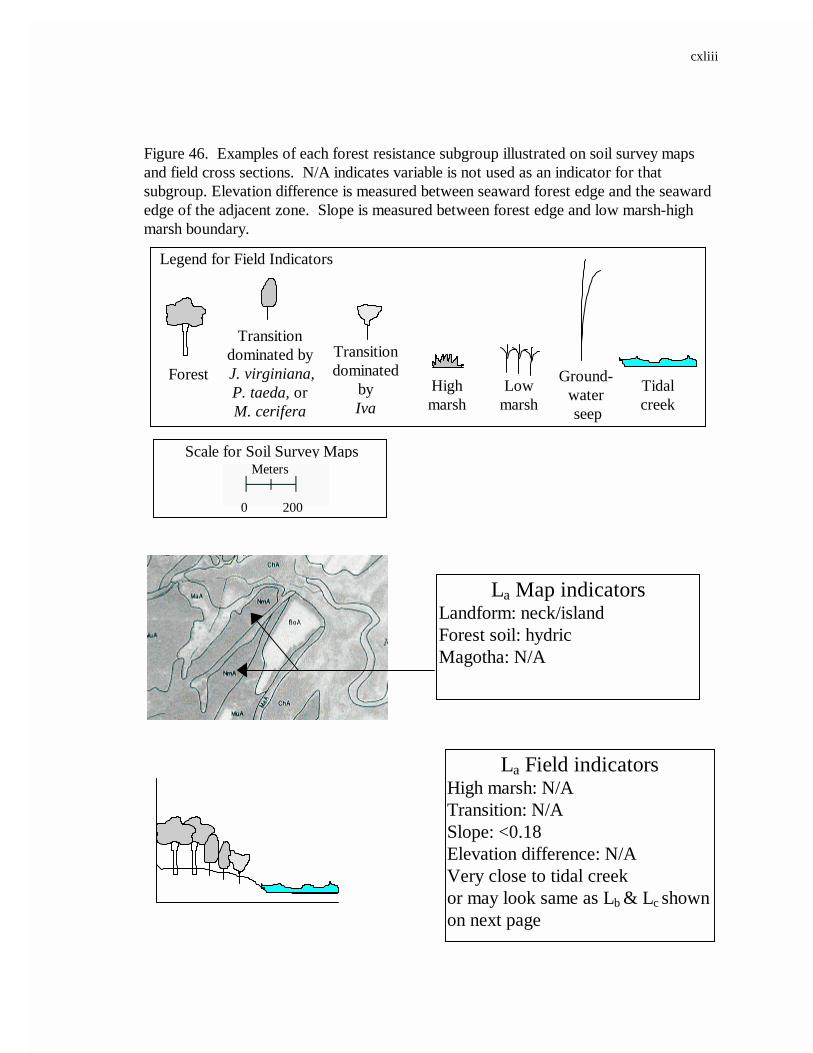
cxliii
Figure 46. Examples of each forest resistance subgroup illustrated on soil survey mapsand field cross sections. N/A indicates variable is not used as an indicator for thatsubgroup. Elevation difference is measured between seaward forest edge and the seawardedge of the adjacent zone. Slope is measured between forest edge and low marsh-highmarsh boundary.
La Map indicatorsLandform: neck/islandForest soil: hydricMagotha: N/A
La Field indicatorsHigh marsh: N/ATransition: N/ASlope: <0.18Elevation difference: N/AVery close to tidal creekor may look same as Lb & Lc shownon next page
Forest
Transitiondominated by J. virginiana,P. taeda, orM. cerifera
Highmarsh
Ground-water seep
Lowmarsh
Transitiondominated
byIva
Legend for Field Indicators
Tidalcreek
Scale for Soil Survey Maps
0 200
Meters

cxliv
Figure 46. Continued.
La, Lb, or Lc
Field indicatorsHigh marsh: very wideTransition: dominated by
Pinus taeda, Juniperusvirginiana, or Myrica cerifera
Slope: N/AElevation difference: N/A
Lb Map indicatorsLandform: InterfluveForest Soil: hydric >100 m wideMagotha: present
Lc Map indicatorsLandform: valleyForest soil: hydricMagotha: N/A

cxlv
Figure 46. Continued.
Ib Field indicatorsHigh marsh: very narrow or absentTransition: dominated by Iva
frutescensSlope: >0.01Elevation: <0.5 m
Ld Map indicatorsLandform: interfluveForest soils: nonhydricMagotha: presentWide distance between 5 and 10 ftcontour interval
Ib Map indicatorsLandform: interfluveForest soils: hydric <35 mMagotha: present
Ld Field indicatorsHigh marsh: <35 mTransition: dominated by Iva
frutescensSlope: <0.01Elevation difference: <0.5 m

cxlvi
Figure 46. Continued.
Ia Map indicatorsLandform: neck/islandForest soil: nonhydricMagotha: N/A
Ic Map indicatorsLandform: valley or interfluveForest soil: nonhydricMagotha: present
Ia or IcField indicators
High marsh: narrow or absentTransition: dominated by Iva
frutescensSlope: N/A for Ia; >0.01 for IcElevation difference: <0.5 m
or
High marsh: narrow (<35 m)Transition: absentSlope: N/A for Ia: >0.01 for IcElevation difference: <0.5 m

cxlvii
Figure 46. Continued.
Hb Map indicatorsLandform: valley or interfluveForest soil: nonhydricMagotha: present
Ha Map indicatorsLandform: valley or interfluveForest soil type: N/AMagotha: absent
Ha or Hb
Field IndicatorsHigh marsh: very narrow (<15 m) or
absentTransition: very narrow (<15 m) or
absentSlope: N/AElevation difference: >0.5 m
orHigh marsh: N/ATransition: absentSlope: N/AElevation difference: >0.5 mGroundwater seep present

cxlviii
Two scenarios exist where map indicators are insufficient to distinguish between
forest resistance groups. First, Ld, Ic and Hb sites all have nonhydric forest soils landward
of MaA soils and, therefore, are not readily distinguishable from each other (Figure 40,
Table 25). Ld sites can be distinguished from Ic and Hb sites if topographic maps are used
because Ld sites have very wide (700 m) 5-10 ft contour intervals whereas Ic and Hb sites
do not. However, Ld sites are rare, so it may be more practical to rely on the use of field
indicators to differentiate between the subgroups. Second, although the 23 field sampled
sites included every variety of soil and landform combination, all lengths of the hydric soil
types were not sampled. All forests sampled with hydric soils >100 m in width were
classified as low resistance and both forests with hydric soils <32.5 m were classified as
intermediate resistance. Because I did not sample any forests with hydric soil widths
mapped between 32.5 and 100 m, I am not sure where the division between I and L
forests would occur between these two widths. For purposes of characterizing maps in
this study, I estimated the division to occur at 50 m. This is closer to the lower width end
of the scale (32.5 m), because generally wide bands of hydric soils indicate low slopes and
poor drainage. Nonetheless, for site determinations, forests with hydric soil map widths
between 32.5 and 100 m should be examined closely in the field.
Using a single field indicator alone is not sufficient to correctly identify resistance
groups because some field indicators overlap among resistance groups, and indicators are
based on field data that did not encompass the full range of field attributes. For example,
both of the wetland island/neck landforms that I sampled lacked a high marsh. It is highly
possible that the larger wetland necks in the Machipongo River watershed appear very

cxlix
similar to the L resistance groups with wide high marsh zones because they have wide
bands of MaA soils. Furthermore, it is possible for L resistant forests to occur in locations
where wide high marsh development would be restricted due to lack of area at lower
elevations. This is especially probable for L forests positioned near ridges of upland
necks. Under these conditions, lack of high marsh does not imply higher resistance. This
scenario was compensated for by using hydric forest soils that fringe valleys, regardless of
MaA soil width, as map indicators for low resistance forest sites. Still, this example
illustrates how a single indicator may lead to placing a given site into the incorrect
resistance group. Furthermore, a transition zone dominated by Iva frutescens is used as
an indicator for identifying several different subgroups spanning all three forest resistance
groups. Therefore, this indicator must be used in conjunction with map indicators for
appropriate resistance group identification.
Landform type alone does not confer resistance because all three forest resistance
groups can occur along both valley and interfluve landforms and L and I resistance groups
occur along necks and islands. Still landforms are useful in identifying resistance groups
because the likelihood of specific L, I, or H physical characteristics occurring within
certain landform positions is predictable. For example, valley landforms develop as marsh
migrates up low gradient streams. Typically forests with hydric soils in a valley setting
have gentle slopes. Therefore, valley landforms with hydric soils in the forest, regardless
of presence of MaA soils, are predicted to have low resistance to state change. In
contrast, forests with hydric soils along interfluve landforms occur in locations with both
gentle to steep slopes. Therefore, within interfluve landforms, the presence and width of

cl
MaA soils are used to estimate land slope (i.e. a wider Magotha series means more gentle
slope).
Islands and necks are in a more advanced stage of drowning than the mainland and
therefore have their own set of resistance indicators. Neck and island landforms do not
have land elevations as high as the mainland and consequently locations with both steep
slopes and high elevations were not detected on them. Because islands and necks
generally lack the criteria necessary for high resistance, forest soil type (hydric vs.
nonhydric) proved to be effective in distinguishing between I and L resistance groups. It
is possible that locations exist along necks that meet high resistance criteria, but none
occurred in any of the locations I sampled.
5.8 Coastal Forest Resistance Classification Procedure
Using map and field indicators, a procedure to rapidly identify a given coastal
forest’s resistance to change in state due to rising sea level was developed. The procedure
has been named Coastal Forest Resistance classification (CFR classification). The CFR
classification procedure consists of two keys in the form of flow charts and supplemental
information that aid in chart use (APPENDIX Q). The key endpoint is a classification for
a given forest as low, intermediate or high in its potential for resisting state change.
Resistance can be expressed at two levels of precision: an assignment to a generic
resistance group (L, I, H) or its position within a specific resistance group. The first part
of Key 1 (Key 1A) uses indicators from soil survey maps, which are published for every
county and are free to the public, to identify a resistance subgroup. The second part of
cli
Key 1 (Key 1B) utilizes field indicators to verify the resistance subgroup identified with
Key 1A. If field indicators do not match the subgroup chosen in Key 1A, the key directs
the user to either a different resistance subgroup or to Key 2. Key 2 is the scoring
procedure that was used to classify sites in this study (Table 4). It requires the most data
but provides the highest accuracy and precision. Individuals desiring the more precise
option are directed to Key 2 from the start. Finally, the CFR classification provides a
statement on the likelihood for forest state change, given a 15 cm rise in sea level, for each
resistance group.
Interpretation of state change rate between resistance groups should be done with
caution. As already mentioned, groups represent different positions along a continuum.
Thus it is possible that overlap in the rate of state change may occur between groups with
different resistance classifications. For this reason, it may be advantageous to use Key 2
to determine whether a site is in a borderline position for its resistance group.
Furthermore, several of the values used in the classification were assumed to be relevant,
rather than based on measurements known to have field significance. Although these
assumed values were useful in partitioning sites into groups, it is not clear how differently
each group will actually respond to rising sea level. Present-day comparisons between
average values of data from forest resistance groups indicate each group is responding
differently to rising sea level. However, these results are based on group averages and so
may or may not represent how an individual site will respond to rising sea level.
Presumably the CFR classification should be applicable in other geographic
locations with similar coastal systems. However, testing of the classification should be

clii
done before implementation. Verification of the CFR classification can be done by cross-
checking map and field indicators for a reasonable number of sites within all forest
resistance subgroups present. If a large number of sites cannot be identified using only
Key 1 then map and/or field indicators should be modified. Modification may consist of
eliminating and/or adding landforms, specific soils series, or indicator species. Because
most of these indicators were generic they should be fairly easily modified. For example,
locations lacking relict sand ridges may use only valley and interfluve landforms as
indicators. Also, specific soil series will likely differ depending on location; however,
generic differentiation between forest soils types (i.e., hydric or nonhydric) and high marsh
soils (Magotha = Natraqualfs) should allow them to be adaptable to similar coastal
systems. Salt marsh species composition is fairly consistent geographically; however,
species indicators used in this study were based on each species level of salt tolerance and
could be changed where necessary.
The CFR classification would not be appropriate for use in determining forest
resistance to state change for all coastal forests. For example, along the Albemarle and
Pamlico Sounds of North Carolina, there are only a few narrow tidal inlets between barrier
islands and the sea. Thus tides are primarily irregular wind tides rather than regular
astronomical tides. Erosion is a large physical force in wind tide (wave) dominated coastal
systems and is not considered in the CFR classification.
Furthermore, unlike forests at the VCR, the resistance of these North Carolina
coastal forests to state change is almost solely a function of their ability to accumulate peat
through autogenic accretion at rates comparable to rising sea level (Moorhead and

cliii
Brinson 1995). Most of these forests are situated at very low elevations, lack a source of
allochthonous sediment, and rest on deep organic soils (Moorhead and Brinson 1995,
Young 1995). Because a platform suitable for marsh migration is lacking, and the
underlying substrate is oxidizable organic matter, these coastal forests convert to open
water rather than undergo the sequence of state changes to low marsh assumed by the
CFR classification, when they are unable to accrete at rates comparable to rising sea level.
Another limitation to the applicability of the CFR classification to other locations is
that it does not incorporate freshwater tidal systems. Because watersheds are so small
along the southern Delmarva Peninsula, freshwater tidal systems do not occur there and
thus were not considered in the study. Unlike coastal forests along the Delmarva
Peninsula where state change is driven by both increased hydroperiod and salt intrusion,
forest conversion to marsh in tidal freshwater systems, results solely from longer
hydroperiods (Orson et al. 1992). For this reason, the CFR classification is not valid in
freshwater tidal systems.
Finally, the CFR classification may not be appropriate for determining forest
resistance to state change on altered sites. Sites in which forest vegetation has been
removed, thinned, burned, or otherwise altered could experience state change more
rapidly than unaltered sites because shading to the forest floor is diminished. Increased
sunlight penetration allows shrubs and herbaceous species to invade earlier than they
normally would. Furthermore, sites that have been hydrologically altered through
ditching, diking, impounding or other activity may not drain as this study predicts and so

cliv
would decrease the certainty of the CFR classification identifying its correct resistance
group.

clv
LITERATURE CITED
Bertness, M. D. 1991. Zonation of Spartina patens and Spartina alterniflora in a New England salt marsh. Ecology 72(1):138-148.
Bertness, M D., L. Gough, and S. W. Shumway. 1992. Salt tolerances and the distribution of fugitive salt marsh plants. Ecology 73(5):1842-1851.
Bertness, M. D., and A. M Ellison. 1987. Determinants of pattern in a New England salt marsh plant community. Ecological Monographs 57(2):129-147.
Braatz, B. V. and D. G. Aubrey. 1987. Recent relative sea-level change in eastern NorthAmerica. pp. 29-46 In Nummedal, D., O. H. Pilkey, and J. D. Howard (eds.) Sea-level Fluctuation and Coastal Evolution. Society of Economic Paleontologists andMineralogists Special Publication No. 41, Tulsa, Oklahoma.
Brinson, M. M, H. D. Bradshaw, and M. N. Jones. 1985. Transitions in forested wetlands along gradients of salinity and hydroperiod. The Journal of Elisha Mitchell Scientific Society 101(2):76-94.
Brinson, M. M., R. R. Christian, and L. K. Blum. 1995. Multiple states in the sea-level induced transition from terrestrial forest to estuary. Estuaries 18(4):648-659.
Broome, S. W., I. A. Mendelssohn, and K. L. McKee. 1995. Relative growth of Spartinapatens (Ait.) Muhl. and Scirpus olneyi Gray occurring in a mixed stand as affectedby salinity and flooding depth. Wetlands 15(1)20-30.
Cahoon, D. R. and J. C. Lynch. 1997. Vertical accretion and shallow subsidence in a mangrove forest of southwestern Florida, USA Mangroves and Salt Marshes. Mangroves and Salt Marshes 00:1-14.
Church, J. A., D. R. Godfrey, and T. J. McDougall. 1991. A model of sea level rise caused by ocean thermal expansion. Journal of Climate 4:438-456.
Clark, J. S. 1986. Coastal forest tree populations in a changing environment, southeastern Long Island, New York. Ecological Monographs 56(3):259-277.
Conner, W. H. and M. Brody. 1989. Rising water levels and the future of southeastern Louisiana swamp forests. Estuaries 12(4)318-323.
Conner, W. H., K. W. McLeod, and J. K. McCarron. 1997. Flooding and salinity effects on growth and survival of four common forested wetland species. Wetlands Ecology and Management 5:99-109.

clvi
Daubenmire, R. 1968. Plant communities: a Textbook of Plant Synecology. Harper and Row Publishers, New York, NY USA.
DeLaune, R. D., S. R. Pezeshki, and W. H. Patrick, Jr. 1987. Response of coastal plants to increase in submergence and salinity. Journal of Coastal Research 3(4):535-546.
DeLaune, R. D., J. A. Nyman, and W. H. Jr. Patrick. 1994. Peat collapse, ponding and wetland loss in a rapidly submerging coastal marsh. Journal of Coastal Research 10(4):1021-1030.
Dott, R. H., Jr. 1992. An introduction to the ups and downs of eustasy. pp. 1-16 InDott, R. H., Jr. (ed.), Eustasy: the Historical Ups and Downs of a Major Geologic Concept. Geological Society of America, Memoir 180. Boulder, Colorado.
Downs, L. L., R. J. Nicholls, S. P. Leatherman, and J. Hautzenroder. 1994. Historic evolution of a marsh island: Bloodsworth Island, Maryland. Journal of Coastal Research 10(4):1031-1044.
Eleuterius, L. N. 1972. The marshes of Mississippi. Castanea 37:153-168.
Fletcher, C. H., H. J. Knebel, and J. C. Kraft. 1990. Holocene evolution of an estuarine coast and tidal wetlands. Geological Society of America Bulletin 102:283-297.
Frey, R. W. and P. B. Basan. 1978. Coastal salt marshes. In R. A. Davis, Jr., (ed.) Coastal Sedimentary Environments. Springer-Verlag Inc. New York, NY.
Gardner, L. R., B. R. Smith, and W. K. Michener. 1992. Soil evolution along a forest-salt marsh transect under a regime of slowly rising sea level, southeastern United States. Geoderma 55:141-157.
Gornitz, V. and S. Lebedeff. 1987. Global sea-level changes during the past century. pp.3-16 In Nummedal, D., O. H. Pilkey, and J. D. Howard (eds.) Sea-levelFluctuation and Coastal Evolution. Society of Economic Paleontologists and Mineralogists Special Publication No. 41. Tulsa, Oklahoma.
Hacker, S. D. and M. D. Bertness. 1995. Morphological and physiological consequences of a positive plant interaction. Ecology 76(7):2165-2175.
Hackney , C. T. and W. J. Cleary. 1987. Saltmarsh loss in southeastern North Carolinalagoons: importance of sea level rise and inlet dredging. Journal of Coastal Research 3(1):93-97.
clvii
Harvey, J. W. and W. E. Odum. 1990. The influence of tidal marshes on upland groundwater discharge to estuaries. Biogeochemistry 10:217-236.
Hayden, B. P., R. D. Dueser, Callahan, J. T., and H. H. Shugart. 1991. Long-Term research at the Virginia Coast Reserve. BioScience 41(5):310-318.
Hmieleski, J.I. 1994. High marsh-forest transitions in a brackish marsh: the effects of slope. MS Thesis. East Carolina University, Greenville, NC. 129 pp.
Intergovernmental Panel on Climate Change (IPCC). 1996. Climate Change 1995 the Science of Climate Change. J. T. Houghton, L. G. Meira Filho, B. A. Callander, N.Harris, A. Kattenberg and K. Maskell (eds.). Cambridge University Press, Great Britain. 572 pp.
Jaworski, A. Z., and J. C. R. Tedrow. 1985. Pedologic properties of New Jersey marshes. Soil Science 139:21-29.
Kana, J. T. W., B. J. Baca, and M. L. Williams. 1987a. Charleston case study. pp 37-60 In James G. Titus (ed.), Greenhouse Effect, Sea Level Rise and Coastal Wetlands.EPA 230-05-86-013. Office of Policy, Planning, and Evaluation, Environmental Protection Agency, Washington, D.C.
Kana, J. T. W., W. C. Eiser, B. J. Baca, and M. L. Williams. 1987b. New Jersey case study. pp. 61-86 In James G. Titus (ed.), Greenhouse Effect, Sea Level Rise and Coastal Wetlands. EPA 230-05-86-013. Office of Policy, Planning, and Evaluation, Environmental Protection Agency, Washington, D.C.
Kastler, J. A. and P. L. Wiberg. 1996. Sedimentation and boundary changes of Virginia coastal salt marshes. Estuarine, Coastal and Shelf Science 42:683-700.
Kayan, I. and J. C. Kraft. 1979. Holocene geomorphic evolution of a barrier-salt marsh system, SW Delaware Bay. Southeastern Geology 20:79-100.
Kaye, C. A. and E. S. Barghoorn. 1964. Late Quaternary sea-level change and coastal rise at Boston, Massachusetts, with notes on the autocompaction of peat. Geol. Soc. Am. Bull. 75:63-80.
Kjerfve, B. 1979. The Santee-Cooper: A study of estuarine manipulations. pp. 45-46 In M. Wiley (ed.), Estuarine Processes, Vol. I. Uses, Stresses and Adaptations to theEstuary. Academic Press, New York, NY.

clviii
Koch, M. S. and I. A. Mendelssohn. Sulphide as a soil phytotoxin: differential responses in two marsh species. Journal of Ecology 77:566-578.
Kurz, H. and K. Wagner. 1957. Tidal Marshes of the Gulf and Atlantic coasts of northern Florida and Charleston, SC. Florida State University Studies 24, Tallahassee, FL, USA.
Lee, J. K., R. A. Park, and P. W. Nausel. 1991. Application of geoprocessing and simulation modeling to estimate impacts of sea level rise on northeastern coastal ofFlorida. Photgrammetric Engineering and Remote Sensing 58:1579-1586.
Meier, M. F. 1990. Reduced (sic) rise in sea level. Nature 343:115.
Miller, W. B., and F. E. Egler. 1950. Vegetation of the Wequetequock-Pawcatuck tidal-marshes, Connecticut. Ecological Monographs 20:143-172.
Mixon, R. B. 1985. Stratigraphic and Geomorphic Framework of Uppermost Cenozoic Deposits in the Southern Delmarva Peninsula, Virginia and Maryland. United States Government Printing Office, Washington, D.C.
Mohanty, S. K. and R. N. Dash. 1982. The chemistry of waterlogged soils. pp. 389-396 In Gopal, B., R. E. Turner, R.G. Wetzel, and D.F. Whighan (eds.) Wetland- Ecology and Management. Natural Institute of Ecology and International Scientific Publications. Jaipur, India.
Moorehead, K. K. and M. M. Brinson. 1995. Response of wetlands to rising sea level in the lower coastal plain of North Carolina. Ecological Applications 5(1):261-271.
Nyman, J. A., R. D. DeLaune, H. H. Roberts, and W. H. Patrick. 1993. Relationship between vegetation and soil formation in a rapidly submerging coastal marsh. Marine Ecological Progress Series 96:269-279.
Oertel, G. F., J. C. Draft, M. S. Kearney and H. J. Woo. 1992. A rational theory for barrier-lagoon development. pp. 77-87 In C. H. Fletcher, III and J. F. Wehniller (eds.). Quaternary Coasts of the United States: Marine and Lacustrine Systems, SEPM Special Publication No. 48. Tulsa Oklahoma.
Oertel, G. F. and H. J. Woo. 1994. Landscape classification and terminology for marsh in deficit coastal lagoons. Journal of Coastal Research 10(4):919-932.
Orson, R., W. Panageotou, and S. P. Leatherman. 1985. Response of tidal salt marshes of the U.S. Atlantic and Gulf coasts to rising sea levels. Journal of Coastal Research 1:29-37.

clix
Orson, R. A., R. L. Simpson, and R. E. Good. 1992. The paleoecological development of a late Holocene, tidal freshwater marsh of the upper Delaware River Estuary. Estuaries 15(2):130-146.
Park, R. A., J. K. Lee, P. W. Mausel and R. C. Howe. 1991. Using remote sensing for modeling the impacts of sea level rise. World Resource Review 3:184-205.
Pearcy, R. W. and Ustin, S. L. 1984. Effects of salinity on growth and photosynthesis of three California tidal marsh species. Oecologica 62:68-73.
Penfound, W. T., and E. S. Hathaway. 1938. Plant communities in the marsh lands of southeastern Louisiana. Ecological Monographs 8:1-56.
Pirazzoli, P. A. 1989. Recent sea-level changes in the North Atlantic. pp. 153-167 In Scott, D. B., P. A. Pirazzolia, and C. A. Honig (eds.) Late Quaternary Sea-Level Correlation and Applications. Kluwer Academic Publishers Dordrecht, Boston and London.
Poland, J. F. and G. H. Davis. 1969. Land subsidence due to withdrawal of fluids. pp. 187- 269 In Review of Engineering Geology II. (Geol. Soc. Amer. ) Boulder, Colorado.
Radford, A. E., H. E. Ahles, and C. R. Bell. 1968. Manual of the Vascular Flora of the Carolinas. The University of North Carolina Press, Chapel Hill. 1183 pp.
Robichaud, A. and Y. Begin. 1997. The effects of storms and sea-level rise on a coastal forest margin in New Brunswick, Eastern Canada. Journal of Coastal Research 13(2):429-439.
Salinas, L. M., R. D. DeLaune and W. H. Patrick. Jr. 1986. Changes occurring along a rapidly submerging coastal area: Louisiana, USA. Journal of Coastal Research 2(3)269:284.
Stasavitch, L. E. 1998. Hydrodynamics of a coastal wetland ecosystem. MS Thesis. East Carolina University, Greenville, NC. 68 pp.
Stevenson, J. D., L. G. Ward and M. S. Kearney. 1986. Vertical accretion in marshes with varying rates of sea level rise. pp. 241-29 In D. A. Wolfe (ed.), Estuarine Variability. Academic Press, Orlando, Florida, USA.
Strahler, A. N. 1957. Quantitative analysis of watershed geomorphology. American Geophysical Union Transactions 38:913-920.

clx
Thien, S. J. 1979. A flow diagram for teaching texture-by-feel analysis. Journal of Agronomic Education 8:54-55.
Titus, J. G. 1987. The Greenhouse Effect, Rising Sea Level and Coastal Wetlands. EPA-230-05-86-013. Office of Policy, Planning and Evaluation, Environmental Protection Agency, Washington, D.C.
Titus, J. G. 1991. Greenhouse effect and coastal wetland policy: how Americans could abandon an area the size of Massachusetts at minimum cost. Environmental Management 15(1):39-58.
Titus, J. G. and V. K. Narayanan, 1995. The Probability of Sea Level Rise. EPA-230-R-95-008. Office of Policy, Planning, and Evaluation Environmental Protection Agency, Washington, D.C.
USDA (United States Department of Agriculture). 1989. Soil Survey of Northampton County, Virginia. Cobb, P. R and D. W. Smith (eds.). Soil Conservation Service and Virginia Polytechnic Institute and State University. 94 pp.
USDA (United States Department of Agriculture). 1994. Soil Survey of Accomac County, Virginia. Peacock, C. D. Jr. and W. J. Edmonds (eds.). Soil Conservation Service and Virginia Polytechnic Institute and State University. 115 pp.
Wigley, T. M. L., and S. C. B. Raper. 1992. Implications for climate and sea level of revised IPCC emissions scenarios. Nature 357:293-300.
Wigley, T. M. L., and S. C. B. Raper. 1993. Future changes in global mean temperature and sea level. pp 111-133 In: R. A. Warrick, E. M. Barrow and T. M. L Wigley (eds.), Climate and Sea Level: Observations, Projections and Implications. Cambridge University Press, Cambridge.
Young, D. R, D. L. Erickson, and S. W. Semones. 1994. Salinity and small-scale distribution of three barrier island shrubs. Canadian Journal of Botany 72:1365-1372.
Young, R. S. 1995. Coastal wetland dynamics in response to sea-level rise: transgression and erosion. Ph.D. Dissertation. Duke University, Durham, NC. 141 pp.

clxi
APPENDIX A. AVERAGE LOW MARSH PERCENT COVERAverage based on three 1m2
quadrats.Species/Cover type Site - Plot Number0-1 meters 2-1 2-2 3-1 3-2 5-1 5-2 8-1 8-2 10-1Spartina alterniflora(>70 cm)
16.7
Spartina alterniflora (40-70 cm)
30.0 22.5 67.5
Spartina alterniflora(<40 cm)
34.2 10.8 37.5 47.5 13.3 39.2 0.8
Distichlis spicata 22.5 37.5 0.8 40.0 0.8Spartina patensSalicornia spp. 10.0 25.8 0.8 0.8Limonium carolinium 0.8 0.8Bare ground 34.2 50.0 61.7 26.7 55.3 41.7 41.7 37.5 44.2Crab burrow 15.0 10.0LitterWrack 12.5 53.3PotholeTotal 100.8 125.0 100.8 114.2 100.3 85.8 103.3 105.0 109.2
1-3 meters 0.0 0.0 0.0 0.0 0.0 0.0 0.0 0.0 0.0
Canopy Cover 0.0 0.0 0.0 0.0 0.0 0.0 0.0 0.0 0.0

clxii
Species/Cover type Site - Plot Number0-1 meters BSN-2 12T-1 12T-2 13-1 13-2 13H-1 13H-2 17-1 17-2S. alterniflora(>70 cm)
S. alterniflora(40-70 cm)
22.5 35.0 0.8
S. alterniflora(<40 cm)
55.8 85.0 35.0 37.5 30.0 12.5 50.0
D. spicata 27.5 0.0 10.0 5.0S. patensSalicornia spp. 13.3 30.0 27.5 21.7 17.5L. caroliniumBare ground 22.5 15.0 37.5 57.5 41.7 65.8 69.2 57.5 47.5Crab burrow 0.8 6.7 15.0LitterWrackPotholeTotal 105.8 100.0 109.2 95.0 111.7 100.0 110.8 105.0 115.8
1-3 meters 0.0 0.0 0.0 0.0 0.0 0.0 0.0 0.0 0.0
Canopy Cover 0.0 0.0 0.0 0.0 0.0 0.0 0.0 0.0 0.0
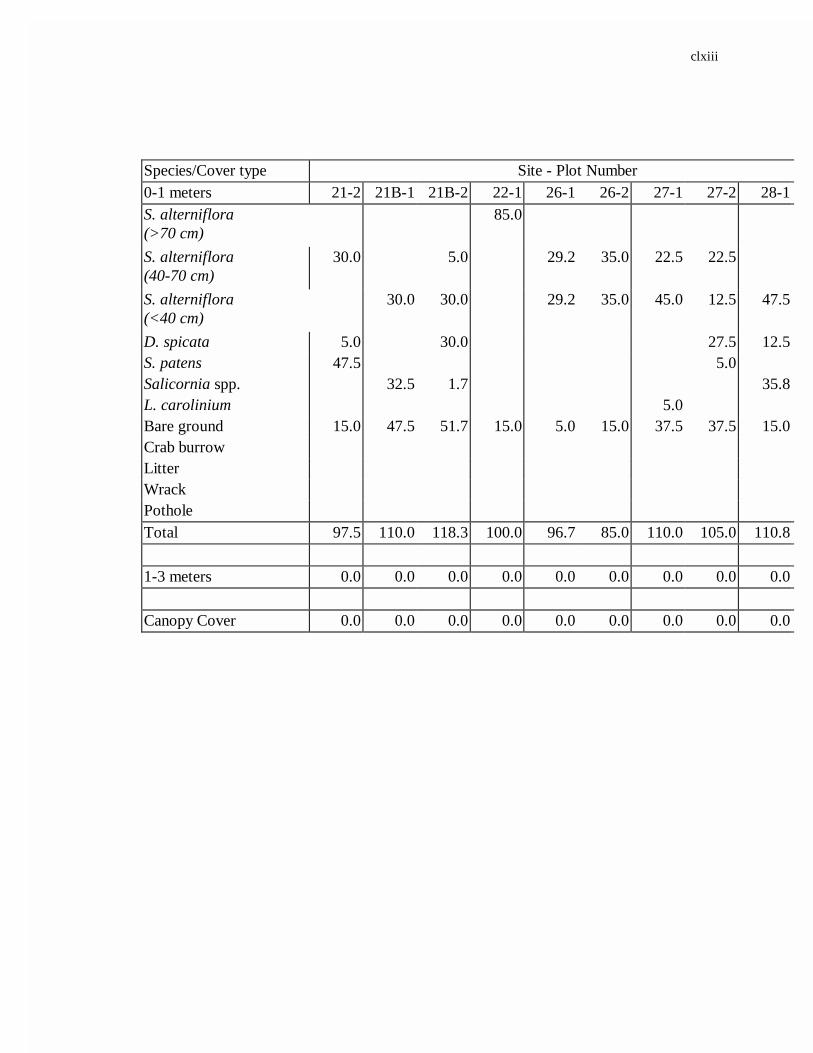
clxiii
Species/Cover type Site - Plot Number0-1 meters 21-2 21B-1 21B-2 22-1 26-1 26-2 27-1 27-2 28-1S. alterniflora(>70 cm)
85.0
S. alterniflora(40-70 cm)
30.0 5.0 29.2 35.0 22.5 22.5
S. alterniflora(<40 cm)
30.0 30.0 29.2 35.0 45.0 12.5 47.5
D. spicata 5.0 30.0 27.5 12.5S. patens 47.5 5.0Salicornia spp. 32.5 1.7 35.8L. carolinium 5.0Bare ground 15.0 47.5 51.7 15.0 5.0 15.0 37.5 37.5 15.0Crab burrowLitterWrackPotholeTotal 97.5 110.0 118.3 100.0 96.7 85.0 110.0 105.0 110.8
1-3 meters 0.0 0.0 0.0 0.0 0.0 0.0 0.0 0.0 0.0
Canopy Cover 0.0 0.0 0.0 0.0 0.0 0.0 0.0 0.0 0.0

164
APPENDIX B. AVERAGE HIGH MARSH PERCENT COVER Average based on three 1m2 quadrats.
Species/Cover type Site - Plot Number0-1 meters 2-1 2-2 2-3 2-4 3-1 3-2 3-3Spartina alterniflora (>70cm)
Spartina alterniflora (<40 cm)
Spartina patens 10.8 17.5 16.7 30.0 29.2 41.7Distichlis spicata 57.5 17.5 26.7 5.8 53.3 57.5 61.7Panicum virgatumSetaria viridisPhragmites australisJuncus roemerianus 39.2 29.2 69.2Juncus gerardiScirpus sp. 5.0Limonium caroliniumSalicornia spp.Atriplex patulaIva frutescens 15.0 0.8Baccharis halimifolia 16.7Erechtites hieracifoliaBorrichia frutescensJuniperus virginianaBare ground 0.8 22.5 12.5 10.0LitterWrack 5.0 12.5 5.0Pothole 12.5Dead shrub 0.8 0.8Woody debrisTotal 89.2 96.7 98.3 101.7 90.0 104.2 103.3
1 - 3 mIva frutescens 0.8 16.7Total 0.8 0.0 0.0 16.7 0.0 0.0 0.0
Canopy Cover 0.0 0.0 0.0 0.0 0.0 0.0 0.0

165
Species/Cover type Site - Plot Number0-1 meters 3-4 9-1 9-2 9-3 11B-1 11B-2 12JA-1 12JA-2S. alterniflora (>70cm)
S. alterniflora(<40 cm)
S. patens 56.7 73.3 95.0 73.3 79.2 5.0 41.7D. spicata 10.0 5.0 26.7 22.5 79.2 5.0 45.8P. virgatumS. viridisP. australisJ. roemerianus 28.3 61.7J. gerardiScirpus sp.L. caroliniumSalicornia spp.A. patulaI. frutescensB. halimifoliaE. hieracifoliaB. frutescensJ. virginianaBare ground 5.0 22.5LitterWrack 0.8 5.0Pothole 30.0 15.0 10.0Dead shrub 5.0Woody debrisTotal 100.8 103.3 100.0 100.0 116.7 94.2 94.2 92.5
1 - 3 mI. frutescens 0.8Total 0.0 0.0 0.0 0.0 0.0 0.0 0.0 0.8
Canopy Cover 0.0 0.0 0.0 0.0 0.0 0.0 0.0 0.0

166
Species/Cover type Site - Plot Number0-1 meters 12JB-1 12JB-2 BFF-1 BFF-2 BFF-3 BSN-1 13-1 13H-1S. alterniflora (>70cm)
S. alterniflora(<40 cm)
12.5
S. patens 29.2 32.5 51.7 57.5 12.5D. spicata 51.7 67.5 35.0 12.5 51.7 15.0 57.5P. virgatumS. viridisP. australisJ. roemerianus 85.0 28.3 73.3J. gerardi 12.5Scirpus sp.L. carolinium 0.8 6.7 6.7Salicornia spp.A. patulaI. frutescens 13.3B. halimifoliaE. hieracifoliaB. frutescensJ. virginianaBare ground 12.5 15.0 15.0LitterWrack 5.0Pothole 37.5 22.5 15.0Dead shrubWoody debrisTotal 93.3 100.0 105.0 118.3 100.8 104.2 110.0 91.7
1 - 3 mI. frutescens
Total 0.0 0.0 0.0 0.0 0.0 0.0 0.0 0.0
Canopy Cover 0.0 0.0 0.0 0.0 0.0 0.0 0.0 0.0

167
Species/Cover type Site - Plot Number0-1 meters 13H-2 17-1 17-2 18-1 21B-1 21B-2 22-1 26-1S. alterniflora (>70cm)
1.7
S. alterniflora(<40 cm)
5.0 15.0
S. patens 27.5 10.0 68.3 28.3 51.7 56.7D. spicata 50.0 40.0 30.0 45.8 67.5 37.5P. virgatum 0.8S. viridisP. australisJ. roemerianusJ. gerardi 47.5Scirpus sp.L. carolinium 5.8Salicornia spp. 0.8A. patula 0.8I. frutescens 30.0 12.5 0.8 40.0 37.5 0.8B. halimifoliaE. hieracifolia 0.8B. frutescens 17.5J. virginianaBare ground 10.0 0.8 13.3Litter 5.0Wrack 5.0 17.5 13.3 0.8PotholeDead shrub 5.0Woody debris 5.0Total 98.3 102.5 82.5 100.8 133.3 105.0 105.8 56.7
1 - 3 mI. frutescens 15.0 12.5Total 0.0 15.0 12.5 0.0 0.0 0.0 0.0 0.0
Canopy Cover 0.0 0.0 0.0 0.0 0.0 0.0 0.0 0.0

168
Species Site - Plot Number0-1 meters 27-1 27-2 27-3 28-1S. alterniflora(>70 cm)
S. alterniflora(<40 cm)
0.8
S. patens 95.0 111.3 55.8 73.3D. spicata 17.5P. virgatumS. viridis 12.5P. australisJ. roemerianusJ. gerardiScirpus sp.L. carolinium 12.5Salicornia spp.A. patula 5.0I. frutescens 13.3 17.5B. halimifoliaE. hieracifoliaB. frutescensJ. virginianaBare groundLitterWrackPothole 0.0 12.5Dead shrubWoody debrisTotal 95.0 137.2 85.8 108.3
1 - 3 mI. frutescens 22.5Total 0.0 0.0 22.5 0.0
Canopy Cover 0.0 0.0 0.0 0.0

169
APPENDIX C. AVERAGE TRANSITION PERCENT COVERAverage based on three 1m2 quadrats.Species/Cover type Site - Plot Number 0 - 1 meters 2-1 3-1 8-1 9-1 10-1 10-2Spartina alterniflora (>70 cm) 13.3Spartina alterniflora (40-70 cm)Spartina patens 17.5 10.0 40.8 12.5 10.8 50.0Distichlis spicata 21.7 5.0Panicum virgatum 35.0Setaria viridisPhragmities australisJuncus roemerianus 12.5 0.8Juncus gerardiScirpus sp. 0.8Limonium caroliniumSalicornia spp.Atriplex patulaTypha sp. 13.3Asclepias incarnataRhus radicans 1.7Parthenocissus quinquefoliaUnidentified graminoid 10.0Iva frutescens 12.5Baccharis halimifolia 0.8Myrica cerifera 40.0Juniperus virginianaPinus taedaPinus serotinaIlex sp. 0.8Bare ground 28.3 47.5Crab burrowLitter 43.3 12.5 5.0 5.0Wrack 0.8 73.3 33.3PotholeDead treeDead shrub 12.5Stump 5.0Woody debris 15.0 5.0 16.7

170
Total 128.3 88.3 100.8 106.7 100.8 88.3
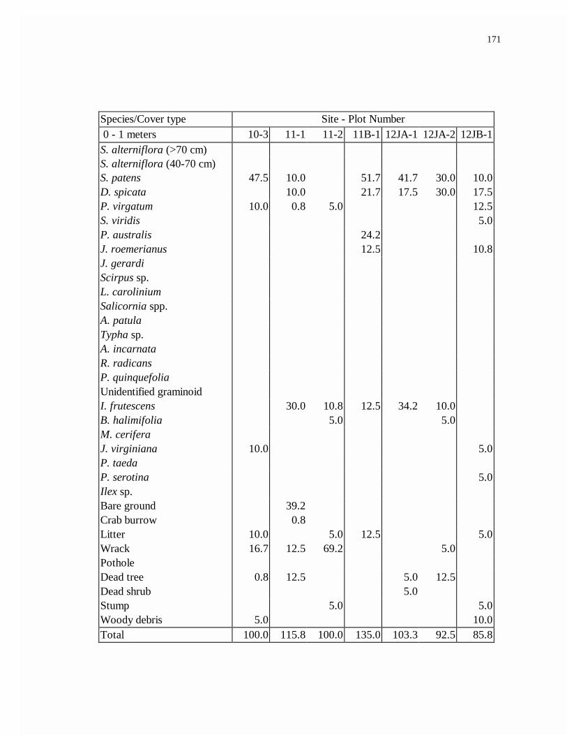
171
Species/Cover type Site - Plot Number 0 - 1 meters 10-3 11-1 11-2 11B-1 12JA-1 12JA-2 12JB-1S. alterniflora (>70 cm)S. alterniflora (40-70 cm)S. patens 47.5 10.0 51.7 41.7 30.0 10.0D. spicata 10.0 21.7 17.5 30.0 17.5P. virgatum 10.0 0.8 5.0 12.5S. viridis 5.0P. australis 24.2J. roemerianus 12.5 10.8J. gerardiScirpus sp.L. caroliniumSalicornia spp.A. patulaTypha sp.A. incarnataR. radicansP. quinquefoliaUnidentified graminoidI. frutescens 30.0 10.8 12.5 34.2 10.0B. halimifolia 5.0 5.0M. ceriferaJ. virginiana 10.0 5.0P. taedaP. serotina 5.0Ilex sp.Bare ground 39.2Crab burrow 0.8Litter 10.0 5.0 12.5 5.0Wrack 16.7 12.5 69.2 5.0PotholeDead tree 0.8 12.5 5.0 12.5Dead shrub 5.0Stump 5.0 5.0Woody debris 5.0 10.0Total 100.0 115.8 100.0 135.0 103.3 92.5 85.8

172
Species/Cover type Site - Plot Number 0 - 1 meters 12JB-2 BFF-1 BFF-2 BSN-1 BSN-2 12T-1 13-1S. alterniflora (>70 cm)S. alterniflora (40-70 cm) 5.0S. patens 10.0 25.0 12.5 17.5 30.0 25.0 22.5D. spicata 5.0 12.5 47.5 12.5 25.0P. virgatum 1.7 21.7 18.3 30.0S. viridis 5.0P. australisJ. roemerianus 33.3 37.5 0.8 0.8J. gerardi 50.8Scirpus sp.L. caroliniumSalicornia spp.A. patulaTypha sp.A. incarnataR. radicansP. quinquefoliaUnidentified graminoidI. frutescens 37.5 34.2 30.0B. halimifolia 17.5 12.5M. cerifera 5.0J. virginiana 0.8P. taeda 5.0 25.0P. serotinaIlex sp.Bare ground 17.5Crab burrow 0.8Litter 40.0 12.5 47.5WrackPotholeDead tree 0.8Dead shrubStump 0.8Woody debrisTotal 100.8 103.3 116.7 102.5 90.0 120.0 104.2

173
Species/Cover type Site - Plot Number 0 - 1 meters 13-2 13H-1 13H-2 18-1 18-2 21-1 21-2S. alterniflora (>70 cm)S. alterniflora (40-70 cm)S. patens 12.5 57.5 22.5 12.5 35.0 5.0 30.0D. spicata 10.0 12.5 0.8P. virgatum 10.8 22.5S. viridis 22.5P. australisJ. roemerianus 5.0J. gerardi 35.0 33.3Scirpus sp.L. carolinium 10.8Salicornia spp.A. patulaTypha sp.A. incarnataR. radicansP. quinquefolia 5.0Unidentified graminoidI. frutescens 22.5 12.5 5.0 45.0 40.0 10.0 25.0B. halimifolia 10.0 5.0 10.0M. ceriferaJ. virginiana 5.0P. taeda 12.5P. serotinaIlex sp.Bare ground 5.0 12.5 5.0Crab burrowLitter 45.0 12.5 5.0 10.8Wrack 1.7Pothole 28.3Dead treeDead shrub 0.8 5.0Stump 5.0Woody debris 17.5 5.0Total 95.8 103.3 107.5 107.5 107.5 95.8 87.5

174
Species/Cover type Site - Plot Number 0 - 1 meters 21B-1 22-1 22-2 22-3 26-1S. alterniflora (>70 cm)S. alterniflora (40-70 cm)S. patens 0.8 73.3 50.0 35.0 17.5D. spicata 5.0 17.5 5.0P. virgatum 17.5 5.0S. viridisP. australisJ. roemerianus 10.0J. gerardiScirpus sp.L. caroliniumSalicornia spp. 0.8A. patula 0.8Typha sp.A. incarnata 13.3R. radicansP. quinquefoliaUnidentified graminoid 10.0I. frutescens 67.5 25.8 17.5 5.0 12.5B. halimifolia 5.0M. cerifera 21.7J. virginianaP. taedaP. serotinaIlex sp.Bare ground 22.5Crab burrowLitter 25.0 0.8 34.2Wrack 5.0 5.0PotholeDead treeDead shrubStump 0.8Woody debrisTotal 103.3 105.8 108.3 86.7 105.8

175
Species Site - Plot Number1 - 3 meters 2-1 3-1 8-1 9-1 10-1 10-2 10-3Phragmities australisIva frutescens 16.7Baccharis halimifolia 4.4 10.0Myrica cerifera 17.5 15.0 67.5Juniperus virginiana 57.5Pinus taedaPinus serotinaIlex sp. 22.5Dead tree 5.0 5.0Dead shrubTotal 21.9 47.5 16.7 67.5 0.0 5.0 62.5
Canopy Cover 22.5 0.0 0.0 44.2 0.0 0.0 17.5
Species Site - Plot Number1 - 3 meters 11-1 11-2 11B-1 12JA-1 12JA-2 12JB-1 12JB-2P. australis 5.0I. frutescens 5.0 5.0B. halimifoliaM. cerifera 22.5 12.5J. virginiana 12.5 5.0 5.0 17.5P. taedaP. serotina 5.0 22.5Ilex sp. 22.5Dead tree 12.5 5.0 17.5 5.0 5.0Dead shrubTotal 12.5 17.5 32.5 22.5 10.0 37.5 52.5
Canopy Cover 0.0 47.5 10.0 5.0 5.0 15.0 38.3

176
Species Site - Plot Number1 - 3 meters BFF-1 BFF-2 BSN-1 BSN-2 12T-1 13-1 13-2 13H-1 13H-2P. australisI. frutescens 17.5 57.5 10.0 5.0B. halimifolia 5.0 22.5M. cerifera 17.5J. virginiana 5.0 50.8P. taeda 5.0 29.2 12.5P. serotinaIlex sp.Dead tree 0.8Dead shrubTotal 10.8 46.7 17.5 55.8 57.5 10.0 22.5 5.0 12.5
Canopy Cover 17.5 30.0 0.0 10.0 5.0 0.0 0.8 0.0 0.0
Species Site - Plot Number1 - 3 meters 18-1 18-2 21-1 21-2 21B-1 22-1 22-2 22-3 26-1P. australisI. frutescens 5.0 33.3 13.3 12.5 29.2 27.5 17.5 13.3 5.0B. halimifolia 30.0 12.5 13.3M. cerifera 35.0J. virginiana 12.5 5.0P. taedaP. serotinaIlex sp.Dead tree 12.5Dead shrub 5.0Total 10.0 33.3 13.3 42.5 29.2 27.5 17.5 50.8 58.3
Canopy Cover 0.0 5.0 0.0 0.0 0.0 0.0 0.0 27.5 33.3

177
APPENDIX D. AVERAGE FOREST PERCENT COVER
Average based on three 1m2
quadrats.Species/Cover type Site - Plot Number0 -1 meters 2-1 2-2 2-3 3-1 3-2 3-3Distichlis spicataPanicum virgatum 10.0Setaria viridisJuncus roemerianusLimonium caroliniumAtriplex patulaAsclepias incarnataHydrocotyle sp.Rhus radicans 0.8Bignonia capreolataParthenocissus quinquefoliaVitis sp. 0.8Smilax bona-nox 1.7 29.2 18.3 10.0 0.8Smilax rotundifoliaUnidentified graminoid 1.7 0.8Iva frutescensMyrica cerifera 5.0 5.0 5.0Erechtites hieracifoliaJuniperus virginianaPinus taedaPinus serotinaPrunus serotina 0.8Ilex opacaNyssa sylvaticaCeltis occidentalisLiquidambar styraciflua 5.0Persea borbonia 0.8 13.3 10.8Aralia spinosaLigustrum sp. 1.7 0.8Quercus phellosBare groundCrab burrowLitter 73.3 53.3 73.3 77.5 67.5 85.0WrackDead treeStump

178
Woody debris 10.0 10.8 13.3 12.5 5.8 15.0Total 101.7 95.0 111.7 110.0 90.0 111.7

179
Species/Cover type Site - Plot Number
0 -1 meters 5-1 5-2 5-3 8-1 9-1 9-2 9-3D. spicataP. virgatum 5.0S. viridis 5.0J. roemerianusL. caroliniumA. patulaA. incarnata 5.0 12.5Hydrocotyle sp. 5.0R. radicans 15.0 10.0 0.8 5.0B. capreolata 10.0 15.0 37.5P. quinquefolia 0.8 5.0Vitis sp. 5.0S. bona-nox 15.0 12.5 17.5S. rotundifolia 5.0Unidentified graminoid 5.0I. frutescensM. cerifera 17.5E. hieracifolia 29.2J. virginianaP. taedaP. serotinaP. serotinaI. opaca 5.0N. sylvatica 0.8C. occidentalis 5.0L. styracifluaP. borboniaA. spinosa 5.0Ligustrum sp.Q. phellosBare ground 12.5 22.5Crab burrowLitter 61.7 47.5 57.5 22.5 51.7 83.3 45.0Wrack 10.0Dead tree 5.0StumpWoody debris 5.0 10.0 34.2 18.3 10.0Total 107.5 105.0 120.0 104.2 103.3 103.3 107.5
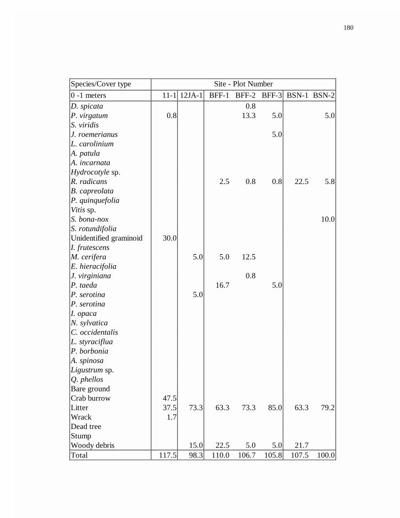
180
Species/Cover type Site - Plot Number
0 -1 meters 11-1 12JA-1 BFF-1 BFF-2 BFF-3 BSN-1 BSN-2D. spicata 0.8P. virgatum 0.8 13.3 5.0 5.0S. viridisJ. roemerianus 5.0L. caroliniumA. patulaA. incarnataHydrocotyle sp.R. radicans 2.5 0.8 0.8 22.5 5.8B. capreolataP. quinquefoliaVitis sp.S. bona-nox 10.0S. rotundifoliaUnidentified graminoid 30.0I. frutescensM. cerifera 5.0 5.0 12.5E. hieracifoliaJ. virginiana 0.8P. taeda 16.7 5.0P. serotina 5.0P. serotinaI. opacaN. sylvaticaC. occidentalisL. styracifluaP. borboniaA. spinosaLigustrum sp.Q. phellosBare groundCrab burrow 47.5Litter 37.5 73.3 63.3 73.3 85.0 63.3 79.2Wrack 1.7Dead treeStumpWoody debris 15.0 22.5 5.0 5.0 21.7Total 117.5 98.3 110.0 106.7 105.8 107.5 100.0

181
Species/Cover type Site - Plot Number
0 -1 meters BSN-3 12T-1 13-1 13-2 21-1 21-2 21-3D. spicataP. virgatum 35.8S. viridisJ. roemerianusL. carolinium 12.5A. patulaA. incarnataHydrocotyle sp.R. radicans 5.0 6.7 10.0 5.8 5.8 0.8B. capreolata 0.8 22.5 15.0 5.0 15.0P. quinquefolia 0.8 0.8 0.8Vitis sp.S. bona-nox 0.8 0.8 1.7 0.8S. rotundifoliaUnidentified graminoidI. frutescens 5.0M. cerifera 12.5E. hieracifoliaJ. virginiana 5.0 16.7P. taedaP. serotinaP. serotinaI. opacaN. sylvaticaC. occidentalis 0.8L. styraciflua 12.5P. borboniaA. spinosaLigustrum sp.Q. phellos 5.0Bare groundCrab burrowLitter 73.3 83.3 51.7 34.2 50.0 73.3 67.5WrackDead tree 0.8StumpWoody debris 17.5 5.0 22.5 12.5 5.0 17.5 22.5Total 99.2 99.2 118.3 107.5 103.3 108.3 105.8
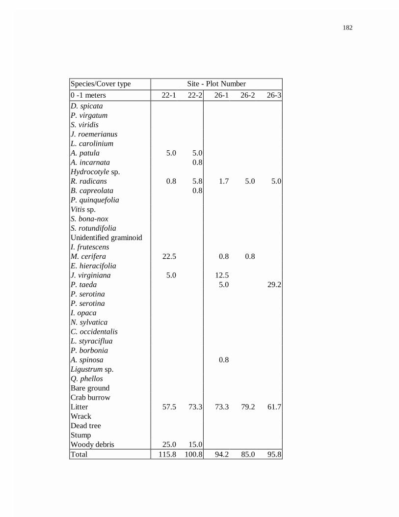
182
Species/Cover type Site - Plot Number
0 -1 meters 22-1 22-2 26-1 26-2 26-3D. spicataP. virgatumS. viridisJ. roemerianusL. caroliniumA. patula 5.0 5.0A. incarnata 0.8Hydrocotyle sp.R. radicans 0.8 5.8 1.7 5.0 5.0B. capreolata 0.8P. quinquefoliaVitis sp.S. bona-noxS. rotundifoliaUnidentified graminoidI. frutescensM. cerifera 22.5 0.8 0.8E. hieracifoliaJ. virginiana 5.0 12.5P. taeda 5.0 29.2P. serotinaP. serotinaI. opacaN. sylvaticaC. occidentalisL. styracifluaP. borboniaA. spinosa 0.8Ligustrum sp.Q. phellosBare groundCrab burrowLitter 57.5 73.3 73.3 79.2 61.7WrackDead treeStumpWoody debris 25.0 15.0Total 115.8 100.8 94.2 85.0 95.8

183
Species Site - Plot Number
1-3 meters 2-1 2-2 2-3 3-1 3-2 3-3 5-1Rhus radicansBignonia capreolataVitis sp. 5.0 5.0Smilax bona-noxSmilax rotundifoliaIva frutescensMyrica cerifera 5.8 34.2 5.0Juniperus virginianaPinus taeda 0.8Pinus serotinaPrunus serotinaIlex opaca 5.0Acer rubrum 0.8 5.0 5.0Nyssa sylvaticaCeltis occidentalisLiquidambar styracifluaPersea borbonia 5.0 5.0Aralia spinosaQuercus phellosLiriodendron tulipiferaDead vines 0.8Dead treeTotal 7.5 0.0 100.0 40.0 15.0 15.0 0.0
Canopy Cover 61.7 61.7 69.2 40.8 47.5 55.8 30.0

184
Species Site - Plot Number
1-3 meters 5-2 5-3 8-1 9-1 9-2 9-3 11-1 12JB-1R. radicans 5.0B. capreolataVitis sp.S. bonanox 17.5S. rotundifoliaI. frutescensM. cerifera 25.0 0.8J. virginiana 10.0 18.3 5.0P. taedaPinus serotina 5.0Prunus serotinaI. opaca 22.5A. rubrumN. sylvatica 5.0 12.5C. occidentalis 12.5L. styraciflua 22.5P. borboniaA. spinosa 12.5Q. phellosL. tulipifera 12.5Dead vinesDead tree 5.0Total 47.5 40.0 17.5 40.0 12.5 5.0 18.3 5.0
Canopy Cover 63.3 77.5 61.7 67.5 73.3 85.0 45.0 67.5
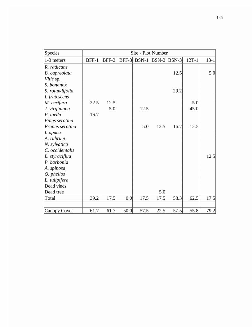
185
Species Site - Plot Number
1-3 meters BFF-1 BFF-2 BFF-3 BSN-1 BSN-2 BSN-3 12T-1 13-1R. radicansB. capreolata 12.5 5.0Vitis sp.S. bonanoxS. rotundifolia 29.2I. frutescensM. cerifera 22.5 12.5 5.0J. virginiana 5.0 12.5 45.0P. taeda 16.7Pinus serotinaPrunus serotina 5.0 12.5 16.7 12.5I. opacaA. rubrumN. sylvaticaC. occidentalisL. styraciflua 12.5P. borboniaA. spinosaQ. phellosL. tulipiferaDead vinesDead tree 5.0Total 39.2 17.5 0.0 17.5 17.5 58.3 62.5 17.5
Canopy Cover 61.7 61.7 50.0 57.5 22.5 57.5 55.8 79.2

186
Species Site - Plot Number
1-3 meters 13-2 21-1 21-2 21-3 22-1 22-2 26-1 26-2 26-3R. radicansB. capreolataVitis sp.S. bonanox 10.0S. rotundifoliaI. frutescens 5.0M. cerifera 5.0 22.5J. virginiana 17.5 27.5 0.8P. taeda 5.0Pinus serotinaPrunus serotinaI. opaca 22.5A. rubrumN. sylvaticaC. occidentalis 28.3 10.0L. styraciflua 22.5P. borboniaA. spinosaQ. phellos 22.5L. tulipiferaDead vinesDead treeTotal 50.8 32.5 22.5 32.5 50.0 10.8 0.0 0.0 0.0
Canopy Cover 32.5 45.8 41.7 73.3 61.7 73.3 73.3 41.7 67.5

187
APPENDIX E. HIGH MARSH WOODY SPECIES DENSITYThere was no basal area in the highmarsh.Species Site - Plot NumberStems/ha 2-1 2-2 2-3 2-4 3-1 3-2 3-3 3-4 5-1 5-2 9-1Iva frutescens 2653 354 442 531Baccharis halimifolia 1592Juniperus virginiana
Total 2653 0 354 2034 531 0 0 0 0 0 0
Species Site - Plot NumberStems/ha 9-2 9-3 11B-1 11B-2 12JA-1 12JA-2 12JB-1 12JB-2 BFF-1 BFF-2 BFF-3I. frutescens 265 1238 2387 265B. halimifoliaJ. virginiana 88Total 265 0 0 0 1238 2476 0 0 265 0 0
Species Site - Plot NumberStems/ha BSN-1 13-1 13H-1 13H-2 17-1 17-2 18-1 21B-1 21B-2 22-1 26-1I. frutescens 973 1326 1655 764 398 2122 1680B. halimifolia 255J. virginiana
Total 0 973 0 1326 1655 1019 398 2122 1680 0 0
Species Site - Plot NumberStems/ha 27-1 27-2 27-3 28-1I. frutescens 105 2315

188
B. halimifolia 1158J. virginiana
Total 105 0 3473 0

189
APPENDIX F. TRANSITION WOODY SPECIES DENSITY AND BASAL AREASpecies Site - Plot NumberStems/ha 2-1 3-1 8-1 9-1 10-1 10-2 10-3 11-1 11-2 11B-1 12JA-1Iva frutescens 88 973 1768 1326Baccharis halimifolia 707 88 177 531 88 88 619Myrica cerifera 1945 619 88Juniperus virginiana 619 1149 1238 177 354 177Pinus taeda 88 177Total 2653 0 0 707 796 1680 1592 1238 354 2122 1945
m2/ha
Iva frutescensBaccharis halimifoliaMyrica ceriferaJuniperus virginiana 2.2 5.2 1.4 6.6Pinus taeda 1.1 5.7Total 0.0 0.0 0.0 0.0 2.2 0.0 6.3 1.4 6.6 5.7 0.0
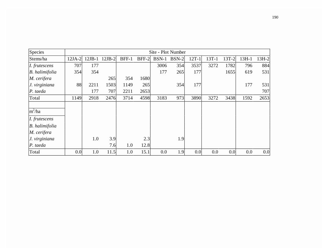
190
Species Site - Plot NumberStems/ha 12JA-2 12JB-1 12JB-2 BFF-1 BFF-2 BSN-1 BSN-2 12T-1 13T-1 13T-2 13H-1 13H-2I. frutescens 707 177 3006 354 3537 3272 1782 796 884B. halimifolia 354 354 177 265 177 1655 619 531M. cerifera 265 354 1680J. virginiana 88 2211 1503 1149 265 354 177 177 531P. taeda 177 707 2211 2653 707Total 1149 2918 2476 3714 4598 3183 973 3890 3272 3438 1592 2653
m2/ha
I. frutescens
B. halimifoliaM. ceriferaJ. virginiana 1.0 3.9 2.3 1.9P. taeda 7.6 1.0 12.8Total 0.0 1.0 11.5 1.0 15.1 0.0 1.9 0.0 0.0 0.0 0.0 0.0

191
Species Site - Plot NumberStems/ha 18-1 18-2 21-1 21-2 21B-1 22-1 22-2 22-3 26-1I. frutescens 3890 2829 4420 1052 4421 4421 1768 1326 177B. halimifolia 884 1368 88 619 884M. cerifera 210 884J. virginiana 526 177 177P. taeda
Total 3890 3714 4420 3157 4421 4509 1768 2122 2122
m2/ha
I. frutescens
B. halimifoliaM. ceriferaJ. virginiana 2.9P. taeda
Total 0.0 0.0 0.0 0.0 0.0 0.0 0.0 2.9 0.0

192
APPENDIX G. FOREST WOODY SPECIES DENSITY AND BASAL AREASpecies Site - Plot NumberStems/ha 2-1 2-2 2-3 3-1 3-2 3-3 5-1Vaccinium corymbosumBaccharis halimifoliaMyrica cerifera 973 88 2829 354 177Juniperus virginianaPinus taeda 442 619 707 796 265Prunus serotina 177 265 354 177Ilex opaca 265Acer rubrum 177 88 265Nyssa sylvatica 88 442 707 88Celtis occidentalis 177 88Liquidambar styraciflua 88 177 177Persea borbonia 177 442 1061Aralia spinosa 265Quercus falcata 88Quercus phellosLiriodendron tulipifera 88Magnolia virginiana
Total 1592 619 884 3537 2211 3360 973
m2/ha
Juniperus virginianaPinus taeda 13.3 15.1 19.6 22.0 8.8Prunus serotina 3.6Ilex opacaNyssa sylvatica 1.9 4.6 3.5 1.2Celtis occidentalis 1.2Liquidambar styraciflua 3.5 2.1 6.7Persea borbonia 1.2Quercus falcata 2.4Liriodendron tulipifera 4.4Total 13.3 15.1 11.4 0.0 27.5 26.7 21.2

193
Species Site - Plot NumberStems/ha 5-2 5-3 8-1 9-1 9-2 9-3 11-1 12JB-1V. corymbosumB. halimifoliaM. cerifera 1768 265 619J. virginiana 354 1061 1768P. taeda 619 531 265 1149P. serotinaI. opaca 88 88 88A. rubrumN. sylvatica 1503 884 531C. occidentalis 354L. styraciflua 88 265P. borboniaA. spinosa 1061Q. falcataQ. phellosL. tulipifera 265 177M. virginiana 177Total 1415 354 442 4244 1857 1061 1061 3537
m2/ha
J. virginiana 1.8 9.3 3.2
P. taeda 17.4 18.4 9.2 13.2P. serotinaI. opacaN. sylvatica 17.7 10.6 12.1C. occidentalis 7.3L. styraciflua 3.2P. borboniaQ. falcataL. tulipifera 15.7 5.7Total 15.7 8.8 7.3 36.9 29.0 21.3 9.3 16.4

194
Species Site - Plot NumberStems/ha BFF-1 BFF-2 BFF-3 BSN-1 BSN-2 BSN-3 12T-1 13-1V. corymbosumB. halimifolia 177M. cerifera 1149 796 442 88J. virginiana 354 177 265 88 442 1592 88P. taeda 2122 1238 707 1415 88 88 177 531P. serotina 88 177 531 531I. opaca 88 354 88 88A. rubrumN. sylvaticaC. occidentalis 884L. styraciflua 88 354P. borboniaA. spinosaQ. falcataQ. phellosL. tulipiferaM. virginiana
Total 3714 2564 884 2211 354 1149 2476 1945
m2/ha
J. virginiana 1.1 1.9 6.9 6.2 1.1
P. taeda 30.0 21.9 14.1 15.2 4.3 4.6 2.1 20.9P. serotina 4.5 0.9 5.3I. opaca 0.9 1.6N. sylvaticaC. occidentalis 2.6L. styraciflua 5.3P. borboniaQ. falcataL. tulipifera
Total 30.9 23.1 14.1 17.1 8.8 14.0 13.6 30.0

195
Species Site - Plot NumberStems/ha 13-2 21-1 21-2 21-3 22-1 22-2 26-1 26-2V. corymbosumB. halimifolia 177 265M. cerifera 354 88 1415 88J. virginiana 177 265 796 88P. taeda 177 177 177 442 354P. serotina 88 88 88I. opaca 442 796 796 531A. rubrumN. sylvatica 88 88 531C. occidentalis 707 354 177L. styraciflua 177P. borboniaA. spinosa 177 442Q. falcataQ. phellos 88L. tulipiferaM. virginiana 88Total 707 1326 1503 1238 707 707 2918 1680
m2/ha
J. virginiana 3.9 1.0 10.1
P. taeda 5.8 7.1 8.4 11.3 13.9P. serotina 1.5I. opaca 4.2 5.3 5.7N. sylvatica 2.0 7.8C. occidentalis 8.0 6.4 5.7L. styracifluaP. borboniaQ. falcataL. tulipifera
Total 8.0 14.0 14.4 15.6 7.3 5.7 21.4 21.7

196
SpeciesStems/ha 26-3V. corymbosumB. halimifoliaM. ceriferaJ. virginianaP. taeda 265P. serotina 265I. opaca 88A. rubrumN. sylvatica 354C. occidentalisL. styracifluaP. borboniaA. spinosa 619Q. falcataQ. phellosL. tulipiferaM. virginiana
Total 1592
m2/ha
J. virginiana
P. taeda 9.4P. serotina 4.9I. opacaN. sylvatica 1.1C. occidentalisL. styracifluaP. borboniaQ. falcataL. tulipifera
Total 15.4

197
APPENDIX H. DENSITY OF LOW MARSH DEAD WOODY VEGETATION COMPONENTSComponent Site - Plot NumberStems/ha 2-1 2-2 3-1 3-2 5-1 5-2 8-1 8-2 10-1 12JA-1 12JA-2 BSN-1Stump 88 88 177 177 177Dead shrub(<1m) 88 88Dead shrub(>1m) 0Dead trees 88Total 88 88 0 0 0 0 0 0 354 177 265 0
Component Site - Plot NumberStems/ha BSN-2 12T-1 12T-2 13-1 13-2 13H-1 13H-2 17-1 17-2 18-1 18-2 21-1Stump 265 88 177Dead shrub(<1m)Dead shrub(>1m)Dead trees 88Total 354 0 88 0 177 0 0 0 0 0 0 0
Component Site - Plot NumberStems/ha 21-2 21B-1 21B-2 22-1 26-1 26-2 27-1 27-2 28-2 28-2StumpDead shrub(<1m)Dead shrub(>1m)Dead treesTotal 0 0 0 0 0 0 0 0 0 0

198
APPENDIX I. DENSITY OF HIGH MARSH DEAD WOODY VEGETATION COMPONENTSComponent Site - Plot
NumberStems/ha 2-1 2-2 2-3 2-4 3-1 3-2 3-3 3-4 9-1 9-2 9-3 11B-1Stump 88Dead shrub(<1m) 177 265 88 88 88Dead shrub(>1m) 88 88 177Dead trees 88Total 0 354 354 88 265 0 88 0 0 88 0 0
Component Site - Plot NumberStems/ha 11B-2 12JA-1 12JA-2 12JB-1 12JB-2 BFF-1 BFF-2 BSN-1 13-1 13H-1 13H-2 17-1Stump 707 707 88 619Dead shrub(<1m) 884 619 88 88 88 265 442 382Dead shrub(>1m) 707 265Dead trees 177 88 88 619Total 0 2476 1680 88 0 177 88 0 88 265 1680 382
Component Site - Plot NumberStems/ha 17-2 18-1 21B-1 21B-2 22-2 26-1 27-1 27-2 27-3 28-1Stump 127Dead shrub(<1m) 382 398 354 1592Dead shrub(>1m) 354 105 1789Dead treesTotal 509 398 354 1592 0 354 105 1789 0 0

199
APPENDIX J. DENSITY OF TRANSITION DEAD WOODY VEGETATION COMPONENTSComponent Site - Plot NumberStems/ha 2-1 3-1 9-1 10-1 10-2 10-3 11-1 11-2 11B-1 12JA-1 12JA-2 12JB-1Stump 177 177 177 177 177 177 707Dead shrub(<1m) 88 265Dead shrub(>1m) 265 88Dead trees 619 442 265 619 619 177 1945 707 531Total 177 0 0 884 619 442 619 796 177 2299 1149 1238
Component Site - Plot NumberStems/ha 12JB-2 BFF-1 BFF-2 BSN-1 BSN-2 12T-1 13-1 13-2 13H-1 13H-2 18-1 18-2Stump 707 707 354 531 442 707 88 265 88 531Dead shrub(<1m) 88 177 88 354 177Dead shrub(>1m) 442 177 177 442 177Dead trees 88 88 177 531Total 796 796 531 1061 442 1061 88 265 707 1061 619 177
Component Site - Plot NumberStems/ha 21-1 21-2 21B-1 22-1 22-2 22-3 26-1Stump 105 88 88 177Dead shrub(<1m) 316 526 619Dead shrub(>1m) 421 265 1857Dead trees 105 88 88 177Total 842 631 88 354 2476 177 354

200
APPENDIX K. DENSITY OF FOREST DEAD WOODY VEGETATION COMPONENTSComponent Site - Plot NumberStems/ha 2-1 2-2 2-3 3-1 3-2 3-3 5-1 5-2 5-3 8-1 9-1Stump 177 265 88 354 177 88 354Dead shrub(<1m)Dead shrub(>1m)Dead trees 354 177 88 265 354 88 177Total 177 619 88 177 88 619 177 0 442 88 531
Component Site - Plot NumberStems/ha 9-2 9-3 11-1 12BJ-1 BFF-1 BFF-2 BFF-3 BSN-1 BSN-2 BSN-3 12T-1Stump 619 707 442 1326 177 442 707 442 88 265 707Dead shrub(<1m)Dead shrub(>1m)Dead trees 265 354 88 88 265 177 177 442 177Total 884 707 88 1680 265 531 973 619 265 707 884
Component Site - Plot NumberStems/ha 13-1 13-2 21-1 21-2 21-3 22-1 22-2 26-1 26-2 26-3Stump 265 177 265 354 88 354 177 177 88Dead shrub(<1m)Dead shrub(>1m)Dead trees 88 177 177 354 354 88 354 88 177 265Total 354 177 354 619 707 177 707 265 354 354

201
APPENDIX L. DEPTH (CM) OF ORGANIC RICH HORIZON BY SAMPLE PLOTI did not auger below 100 cm. Therefore, sites reported as 100 cm depth may actually have organic richsoils at greaterdepths. L = low marsh, H = high marsh, T = transition, F= forest
Zone- Plot NumberSite L-1 L-2 H-1 H-2 H-3 H-4 T-1 T-2 T-3 F-1 F-2 F-32 0 0 16 15 8 10 6 5 6 63 100 100 100 100 75 40 5 6 5 55 100 100 0 0 08 15 0 0 09 30 45 30 5 5 5 210 0 2 2 211 0 0 011B 50 40 512JA 0 0 0 0 9 1312JB 4 25 8 6 5BFF 10 10 10 10 3 3 4BSN 18 5 10 0 0 6 2 112T 10 0 0 013 5 10 5 10 6 0 013H 0 0 0 0 4 317 100 35 0 418 70 35 20 8 021 100 56 40 4 2 0 221B 80 20 0 0 022 60 30 0 0 0 0 0

202
26 90 90 15 10 5 3 027 100 100 100 100 10028 35 45 0

203
APPENDIX M. PERCENT SOIL ORGANIC MATTER BY ZONE Subsurface is the first 10 cm of the second deepest horizon.
0-10 cm SubsurfaceSite Low
marshHighmarsh
Transition Forest Lowmarsh
Highmarsh
Transition Forest
2 7.9 21.7 45.7 60.0 2.9 5.8 7.6 3.13 21.9 24.6 14.9 30.3 30.2 18.8 3.0 6.75 18.1 1.9 20.6 2.28 6.7 1.8 5.0 2.3 2.0 3.09 54.3 15.0 9.3 10.8 2.9 4.110 11.7 4.5 1.9 2.211 7.5 20.7 3.6 5.811B 59.5 26.0 10.2 5.212JA 8.5 7.812JB 47.6 28.9 62.7 24.8 8.1 11.4BFF 33.7 11.0 24.2 15.7 3.6 4.3BSN 30.9 15.1 5.1 13.1 2.2 5.8 1.9 3.712T 9.8 13.3 21.3 3.0 6.2 3.013 7.8 12.2 11.1 17.5 4.5 5.1 3.4 2.313H 3.1 9.3 10.9 3.0 3.4 2.617 26.4 2.5 4.4 1.918 31.8 42.0 5.1 4.8 6.0 2.121 47.3 17.5 6.5 41.2 3.9 2.321B 42.8 8.6 5.8 9.1 1.9 1.722 24.0 15.8 9.6 6.6 16.4 13.4 2.8 2.726 45.5 61.9 18.2 1.2 38.7 4.9 7.5 3.127 32.9 50.2 33.6 47.8

204
28 16.8 5.4 13.0 1.9
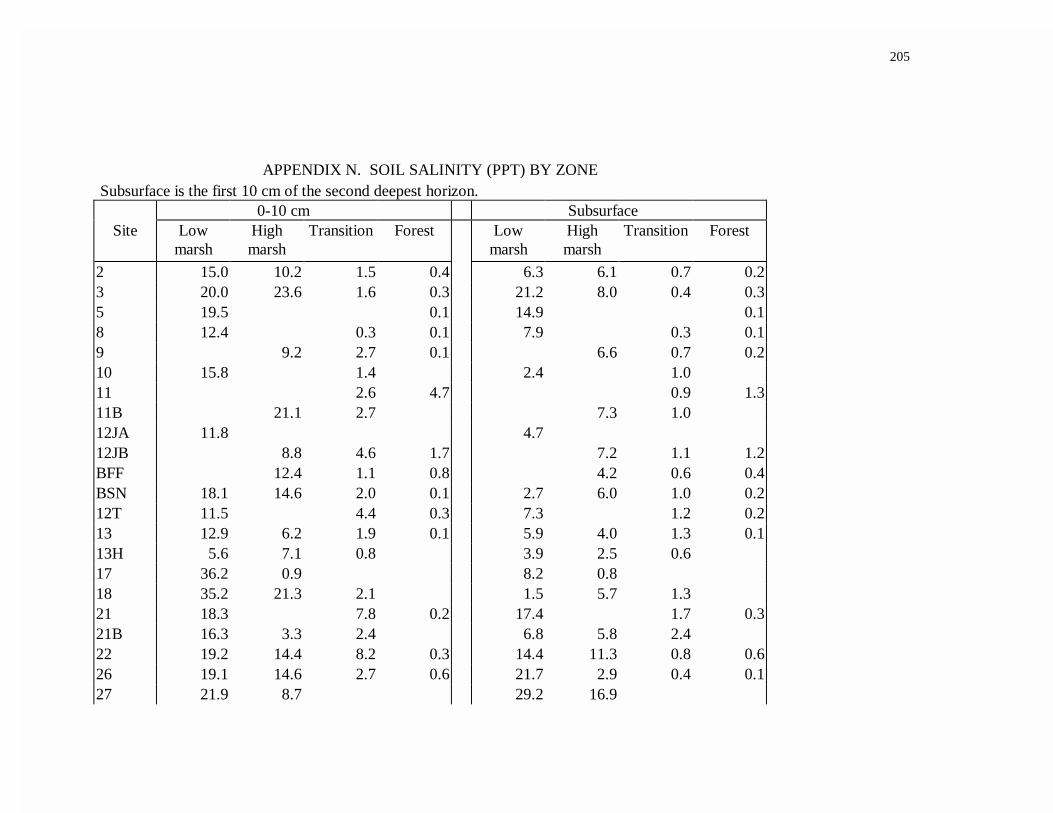
205
APPENDIX N. SOIL SALINITY (PPT) BY ZONE Subsurface is the first 10 cm of the second deepest horizon.
0-10 cm SubsurfaceSite Low
marshHighmarsh
Transition Forest Lowmarsh
Highmarsh
Transition Forest
2 15.0 10.2 1.5 0.4 6.3 6.1 0.7 0.23 20.0 23.6 1.6 0.3 21.2 8.0 0.4 0.35 19.5 0.1 14.9 0.18 12.4 0.3 0.1 7.9 0.3 0.19 9.2 2.7 0.1 6.6 0.7 0.210 15.8 1.4 2.4 1.011 2.6 4.7 0.9 1.311B 21.1 2.7 7.3 1.012JA 11.8 4.712JB 8.8 4.6 1.7 7.2 1.1 1.2BFF 12.4 1.1 0.8 4.2 0.6 0.4BSN 18.1 14.6 2.0 0.1 2.7 6.0 1.0 0.212T 11.5 4.4 0.3 7.3 1.2 0.213 12.9 6.2 1.9 0.1 5.9 4.0 1.3 0.113H 5.6 7.1 0.8 3.9 2.5 0.617 36.2 0.9 8.2 0.818 35.2 21.3 2.1 1.5 5.7 1.321 18.3 7.8 0.2 17.4 1.7 0.321B 16.3 3.3 2.4 6.8 5.8 2.422 19.2 14.4 8.2 0.3 14.4 11.3 0.8 0.626 19.1 14.6 2.7 0.6 21.7 2.9 0.4 0.127 21.9 8.7 29.2 16.9
206
28 16.7 2.6 19.1 1.2
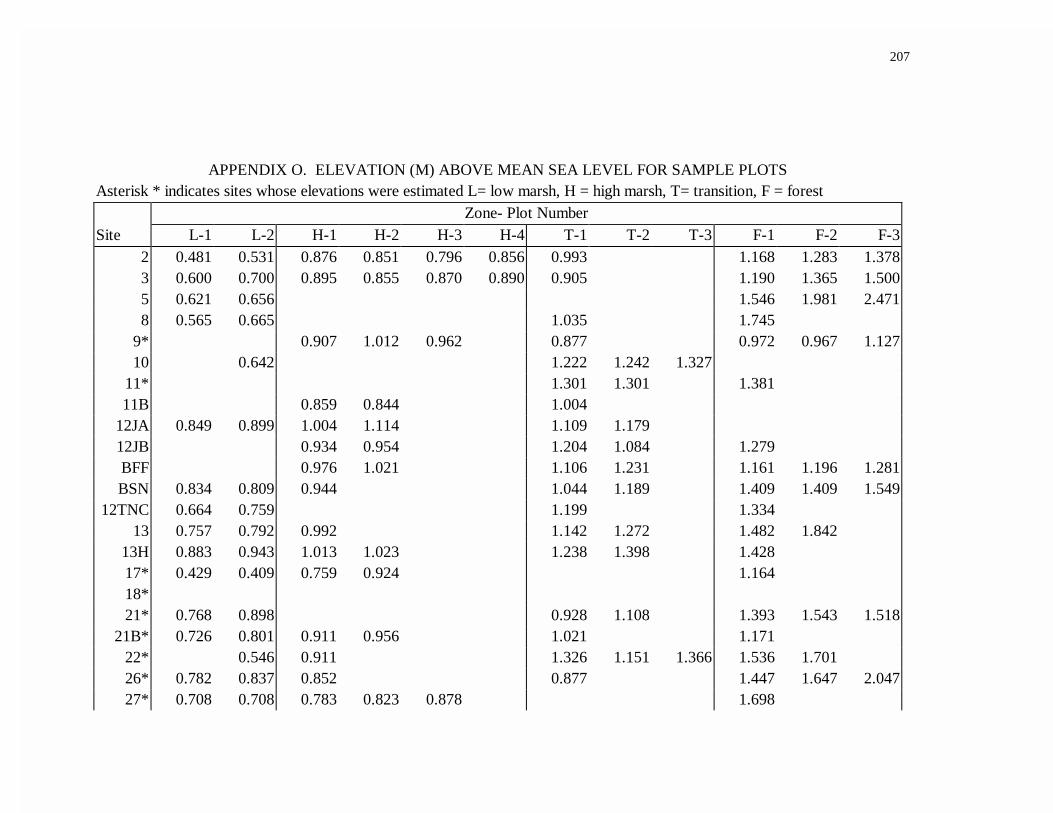
207
APPENDIX O. ELEVATION (M) ABOVE MEAN SEA LEVEL FOR SAMPLE PLOTSAsterisk * indicates sites whose elevations were estimated L= low marsh, H = high marsh, T= transition, F = forest
Zone- Plot NumberSite L-1 L-2 H-1 H-2 H-3 H-4 T-1 T-2 T-3 F-1 F-2 F-3
2 0.481 0.531 0.876 0.851 0.796 0.856 0.993 1.168 1.283 1.3783 0.600 0.700 0.895 0.855 0.870 0.890 0.905 1.190 1.365 1.5005 0.621 0.656 1.546 1.981 2.4718 0.565 0.665 1.035 1.745
9* 0.907 1.012 0.962 0.877 0.972 0.967 1.12710 0.642 1.222 1.242 1.327
11* 1.301 1.301 1.38111B 0.859 0.844 1.004
12JA 0.849 0.899 1.004 1.114 1.109 1.17912JB 0.934 0.954 1.204 1.084 1.279BFF 0.976 1.021 1.106 1.231 1.161 1.196 1.281BSN 0.834 0.809 0.944 1.044 1.189 1.409 1.409 1.549
12TNC 0.664 0.759 1.199 1.33413 0.757 0.792 0.992 1.142 1.272 1.482 1.842
13H 0.883 0.943 1.013 1.023 1.238 1.398 1.42817* 0.429 0.409 0.759 0.924 1.16418*21* 0.768 0.898 0.928 1.108 1.393 1.543 1.518
21B* 0.726 0.801 0.911 0.956 1.021 1.17122* 0.546 0.911 1.326 1.151 1.366 1.536 1.70126* 0.782 0.837 0.852 0.877 1.447 1.647 2.04727* 0.708 0.708 0.783 0.823 0.878 1.698

208
28* 0.672 0.657 0.787 1.122

APPENDIX P. ZONE WIDTH (M) MEASURED IN THE FIELDBlank cells represent zones not sampled, and cells with zero representmissing zones.
ZoneSite Low
marshHighmarsh
Transition Forest
2 24 100 7 363 24 176 4 365 24 0 0 368 24 0 3 129 157 4 3610 12 0 5511 0 20 1211B 72 812JA 24 6 2612JB 202 42 12BFF 99 30 36BSN 24 8 21 3612T 24 0 6 913 24 14 20 1813H 24 32 1817 24 20 018 24 4 1821 24 0 22 3621B 24 33 1222 12 8 60 1826 24 6 6 3627 24 33 028 24 6 0

ccx
APPENDIX Q. COASTAL FOREST RESISTANCE CLASSIFICATIONWORKSHEETS
STEPSFOR DETERMINATION OF FOREST RESISTANCE TO STATE CHANGE
LOCATE SITE ON SOIL SURVEY
CHOOSE LEVELOF PRECISION DESIRED
LESS PRECISE Forest resistance classification
only:Low, Intermediate, or High
MORE PRECISEScore indicating position within
the forest resistance group: Low,Intermediate, or High
FOLLOW FLOW CHARTSIN KEY 1
BEGINNING WITH KEY 1Ato determine forest resistance group.You may be sent to key 2 if your site
does not match one in this study
FOLLOW STEPSIN KEY 2
to determine score and forestresistance group
INTERPRETATION OF FOREST RESISTANCE CLASSIFICATIONLOW: forest is very likely to begin conversion to marsh with a 15 cm
rise in sea level.
INTERMEDIATE: forest is somewhat likely to begin conversion to marsh with a 15 cm rise in sea level.
HIGH: forest is very unlikely to begin conversion to marshwith a 15 cm rise in sea level.

ccxi
Key 1A. Map indicators. Refer to Key 1A Supplement 1 and 2 for landform descriptionsand a list of forest (hydric and nonhydric) and marsh soil series. Magotha (MaA) soilsoccur in the high marsh and transition zones. Width of forest soil is measuredperpindicular to the coastline.
Choose landform that coastal forest fringes
Valleycoastal forestfringes marshsoils in valley
Neck or Islandcoastal forest
occurs on islandor neck
Interfluvecoastal forestfringes marsh
occurringbetweenvalleys
Hydric soils>100 m width
Hydric soils35-100 m width
Hydric soils <35 m width
Nonhydric
Forest SoilType
Magotha(MaA) Soil Go to:
Hydric
Nonhydric absent
present
present
absent
Ha -Key 1B
Ic -Key 1B
Lc -Key 1B
Lb -Key 1B
Ha -Key 1B
present
absent
present
absent
present
absent
Ha -Key 1B
Ic -Key 1B
Ha -Key 1B
Ha -Key 1B
Key 2
Ha -Key 1B
Hydric
Nonhydric Ia -Key 1B
La -Key 1B

ccxii
Key 1A. Supplement 1. LANDFORMS
* The boundary between the valley mouth and interfluve is not always distinct. When inquestion, assume valley when forest soils are hydric. If forest soils are nonhydric theneither landform will give the same classification results.
Land
Marsh
Creek
VALLEY - Land surroundingmarsh contained within a valley.
INTERFLUVE -portion of land positionedbetween valleys.
NECK - land surrounded bymarsh on three sides with aconnection to the mainland. Necksare remnant Bell Neck ridges andoccur between Holt Creek inNorthampton county andNicciwampus creek in Accomaccounty.
ISLAND - landcompletely severed from themainland and surrounded bymarsh on all sides. Islandsare remnant Bell NeckRidges.
Valley perimeter
Neck perimeter
Interfluve perimeter
Island perimeter

ccxiii
Key 1A. Supplement 2. SOIL SERIES
SEASIDE SOIL SERIES OF NORTH HAMPTON AND ACCOMAC COUNTIES
FOREST SOILS FOREST SOILS MARSH SOILSNonhydric Hydric Hydric
Assateague (Atd) Arapahoe (ArA or AhA) Chincoteague (ChA)Bojac (BkA, BoA, Bhb) Camocca (CaA) Magotha (MaA)Fisherman (FhB) Dragston (DrA)Molena (MoA) Nimmo (NmA)Munden (MuA) Polawana (PoA)Seabrook (SeA)Udorthents, Udipsamments(UpD)

ccxiv
Key 1B Field indicators. N/A = not an indicator for that group. Use information fromthe tables below to help with resistance group identification. If a resistance group isreached return to instructions for interpretation if not go to Key 2 for more datacollection.
ZONE (ECOSYSTEM STATES) DESCRIPTIONS FOR FIELD IDENTIFICATION
Zone (ecosystem state) DescriptionForest dominated by trees and lacking marsh grasses
Transition dominated by shrubs or small trees and marshgrasses present
Groundwater seep dominated by Phragmites australis or Scirpusspp.
High marsh dominated by marsh grasses Spartina patens orDistichlis spicata or rush Juncus roemerianus;shrubs, if present, cover < 50 % of area
Low marsh dominated by marsh grass, Spartina alterniflora
FIELD MEASUREMENTS
Measure Description (unless otherwise stated)
Slope =elevation difference (m) between seaward forest edge
and landward low marsh edgedistance (m) between seaward forest edge and
landward low marsh edge
Elevation difference = elevation difference (m) between seaward end of forestand seaward end of zone adjacent to forest

ccxv
Key 1B. Continued.
La
High marsh: N/ATransition: N/ASlope: <0.18Elevation difference: N/AForest position: close to tidal creek (w/in 55 m)
High marsh: wide (>50 m)Transition: dominated by Pinus taeda,
Juniperus virginiana or Myrica ceriferaSlope: N/AElevation difference: N/A
LOW
Go to Key 2
Lb
orLc
LOW
YES
YES
Go to Key 2NO
NO
LOWLd
High marsh: N/ATransition: dominated by Iva frutescensSlope: <0.01Elevation difference: <0.15 m
YES
Go to Key 2NO
High marsh: very narrow <15 m or absent Transition: very narrow <15 m or absentSlope: N/AElevation difference: >0.5 m
Ia
High marsh: N/ATransition: absentSlope: N/AElevation difference: >0.5 mGroundwater seep: present
High marsh: narrow (<35m) or absentTransition: dominated by Iva frutescens
or absentSlope: N/AElevation difference: <0.40 m
INTERMEDIATEYES
NO Go to Key 2
Ib
orIc
High marsh: narrow (<35 m) or absentTransition: dominated by Iva frutescens
or absentSlope: >0.01Elevation difference: <0.4 m
NO
YES INTERMEDIATE
Go to Hb
Resistance toState Change
Go to Ld
HIGHYES
NO
Go to Key 2
HIGHYES
NO
Ha
orHb
All indicators must be present to choose “YES”
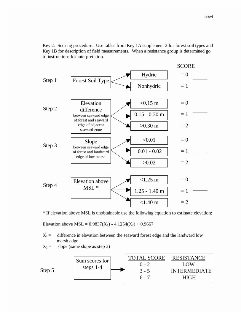
ccxvi
Key 2. Scoring procedure. Use tables from Key 1A supplement 2 for forest soil types andKey 1B for description of field measurements. When a resistance group is determined goto instructions for interpretation.
* If elevation above MSL is unobtainable use the following equation to estimate elevation:
Elevation above MSL = 0.9837(X1) - 4.1254(X2) + 0.9667
X1 = difference in elevation between the seaward forest edge and the landward low marsh edge
X2 = slope (same slope as step 3)
Step 1
Step 2
Step 3
Step 4
Forest Soil TypeHydric
Nonhydric
Elevationdifference
between seaward edgeof forest and seaward
edge of adjacentseaward zone
<0.15 m
0.15 - 0.30 m
>0.30 m
Slopebetween seaward edgeof forest and landward
edge of low marsh 0.01 - 0.02
>0.02
<0.01
Elevation aboveMSL *
<1.25 m
1.25 - 1.40 m
<1.40 m
SCORE
TOTAL SCORE RESISTANCE0 - 2 LOW3 - 5 INTERMEDIATE6 - 7 HIGH
= 0
= 1
= 0
= 1
= 2
= 0
= 1
= 2
= 0
= 1
= 2
Step 5
Sum scores forsteps 1-4

ccxvii