Liquidity Regulation and Credit Booms:Theory and Evidence from China∗

Kinda HachemChicago Booth and NBER

Zheng Michael SongChinese University of Hong Kong

First Draft: January 2015This Draft: February 2017

Abstract

Many countries try to mitigate business cycle fluctuations by regulating the ac-tivities of their banks. We develop a theoretical framework to study the endogenousresponse of the banking sector and the implications for the aggregate economy. Underfairly mild conditions, we find that stricter liquidity standards can generate unintendedcredit booms as attempts to arbitrage the regulation change the allocation of savingsacross banks and the allocation of lending across markets. We then apply our frame-work to study recent events in China. We show that a regulatory push to increasebank liquidity and cap loan-to-deposit ratios in the late 2000s accounts for one-third ofChina’s unprecedented credit boom and one-half of the increase in interbank interestrates over the same period. We also find strong empirical support for the cross-sectionaldifferences between big and small banks predicted by the model.

∗This paper supersedes an earlier version which circulated as “Liquidity Regulation and UnintendedFinancial Transformation in China.”We thank Chang-Tai Hsieh and Anil Kashyap for several helpful con-versations. We also thank Jeff Campbell, Jon Cohen, Doug Diamond, Gary Gorton, John Huizinga, RandyKroszner, Mark Kruger, Brent Neiman, Gary Richardson, Rich Rosen, Ben Sawatzky, Martin Schneider,Aleh Tsyvinski, Harald Uhlig, and Xiaodong Zhu as well as Viral Acharya, Sofia Bauducco, and Jun Qian.Special thanks to Mingkang Liu and the other bankers and regulators who guided us through some of theinstitutional details in China. We are also grateful to seminar and conference participants at MinnesotaCarlson, CUHK, Queen’s University, Bank of Canada, Chicago Booth, Nankai, HKU, HKUST, Tsinghua,Fudan University, FRB Minneapolis, NUS, IMF, US Treasury (OFR), the 2015 Symposium on EmergingFinancial Markets, SED 2015, NBER Summer Institute 2015 (Monetary Economics), FRB Chicago, the IMF-Princeton-CUHK Shenzhen Conference, the April 2016 NBER IFM meeting, the First Research Workshopon China’s Economy, the May 2016 NBER Chinese Economy meeting, the 2016 China Financial ResearchConference, the 2nd Annual BOC-UofT-Rotman Conference on the Chinese Economy, and the Central Bankof Chile’s Macroeconomic Policy Workshop on the Chinese Economy. Financial support from Chicago Boothand CUHK is gratefully acknowledged.

1

1 Introduction

Seeking to mitigate booms and busts, many countries regulate bank lending in relation

to the quantity and composition of bank liabilities. Proponents insist that business cycle

fluctuations would be more severe without these regulations but policy-makers remain wary

of unintended consequences. In the words of Stanley Fischer, Vice Chairman of the U.S.

Federal Reserve, a “tightening in regulation of the banking sector may push activity to other

areas —and things happen.”Exactly what happens, Fischer argues, is diffi cult to predict with

existing models as there is limited theoretical work on the interactions between regulated

and unregulated institutions and the economic incentives that drive them.1 In this paper,

we develop a theoretical framework which helps fill the gap between existing models and the

models requested by policy-makers.

The need for such a framework is underscored by recent events in China, one of the

world’s largest and most rapidly growing economies. Between 2007 and 2014, the ratio

of debt to GDP in China exploded from 110% to 200%. The ratio of private credit to

private savings, sometimes a more conservative gauge, also rose markedly from 65% to 75%

over the same period. This credit boom appears to have occurred on the heels of stricter

regulation. Around 2008, Chinese regulators began enforcing an old but hitherto neglected

loan-to-deposit cap which forbade banks from lending more than 75% of their deposits to non-

financial borrowers. Loans to non-financials are among the least liquid financial assets on a

bank’s balance sheet, making loan-to-deposit caps akin to liquidity regulation. The objective

of the enforcement action in China was to increase bank liquidity and keep credit growth

under control, opening the door to three hypotheses. One hypothesis is that enforcement

was successful: China’s credit boom would have been even larger had regulators not begun

enforcing the loan-to-deposit cap. Another hypothesis is that enforcement was of limited

importance, perhaps because loan-to-deposit rules were not binding on the true drivers of

credit growth. A third hypothesis is that enforcement failed: by enforcing the loan-to-

deposit cap, regulators actually helped create the credit boom, a particularly egregious type

of unintended consequence.

Of these hypotheses, the third is the most surprising and requires a coherent theory of

how a policy that sounds like it will decrease credit growth —or, at worst, leave credit growth

unchanged —leads instead to a credit boom. The theoretical framework we develop in this

paper allows us to evaluate the viability of the third hypothesis as an equilibrium result.

We find that it emerges as an equilibrium under fairly mild conditions and accounts for a

1Speech delivered at the 2015 Financial Stability Conference, Washington D.C., December 3,www.federalreserve.gov/newsevents/speech/fischer20151203a.htm.

2

quantitatively important fraction of the Chinese experience. In other words, stricter liquidity

standards unintentionally helped create China’s recent credit boom.

Although China is the setting for our quantitative analysis, none of the ingredients in the

theory are uniquely Chinese. Our framework is one where banks engage in maturity trans-

formation, borrowing short and lending long. This leaves them vulnerable to idiosyncratic

withdrawal shocks, giving rise to an ex post interbank market where banks with insuffi cient

liquidity can borrow from banks with surplus liquidity at an endogenously determined price.

We add to this environment two features. First, banks can choose whether to manage all

of their activities on a regulated balance sheet or whether to move some activity to a less

regulated off-balance-sheet vehicle. We use the term “off-balance-sheet vehicle” to mean

any accounting maneuvers banks can legally take to present more favorable balance sheets.

Accounting rules are typically one step behind the maneuvers innovated by banks so we want

to build a model which takes this feature of the real world seriously.2 Second, the economy

is served by both big and small banks, namely a big bank that internalizes the effects of its

choices on other actors and a continuum of small banks that do not. A recent line of work

by Corbae and D’Erasmo (2013, 2014) also distinguishes explicitly between big and small

banks, albeit in a different environment with exogenous pricing on the interbank market and

no possibility of off-balance-sheet vehicles.

We show that enforcing a loan-to-deposit cap in our framework can lead to a credit boom.

The mechanism we uncover has two parts.

First, the loan-to-deposit cap leads small banks to engage in regulatory arbitrage. Our

model predicts that the small banks have higher loan-to-deposit ratios than the large bank

and are thus disproportionately affected by enforcement of the cap. In response, they find it

optimal to offer a new savings instrument and manage the funds raised by this instrument

in an off-balance-sheet vehicle that is not subject to the loan-to-deposit cap and that can

therefore make the loans the bank cannot make without violating the cap. This consti-

tutes shadow banking: it achieves the same type of credit intermediation as a regular bank

without appearing on a regulated balance sheet. It also achieves the same type of maturity

transformation as a regular bank, with long-term assets financed by short-term liabilities.

Second, the shadow banking activities of the small banks elicit a response from the big

bank. Specifically, the big bank views these initiatives as a challenge to its profits. As small

banks push to attract savings into off-balance-sheet instruments, they raise the interest rates

on these instruments above the rates on traditional deposits and poach funding from the big

2Off-balance-sheet activities still exist under U.S. GAAP. To this point, it is estimated that U.S. bankswould be roughly 20-25% larger under IFRS standards. This is a sizeable magnitude, especially since IFRSstandards are not themselves immune.

3

bank. We show that the big bank’s equilibrium response is both to issue its own high-return

savings instruments and to modify its interbank behavior. While the first of these responses is

intuitive, the second requires elaboration. Given that maturity mismatch extends to shadow

banking, the interbank market remains an important source of emergency liquidity for small

banks. Therefore, by making the interbank market less liquid, the big bank can compel

small banks to behave less aggressively in their quest for off-balance-sheet business and thus

lessen the extent to which they poach deposits. Since small banks do not internalize the

effects of their choices, they are price-takers on the interbank market. The big bank, on the

other hand, understands that it is large enough to shift the demand for liquidity relative to

the supply, leading to sudden changes in the market-clearing interbank interest rate. With

a central bank that does not automatically offset all such changes — examples abound in

emerging economies and U.S. monetary history —the big bank has ex ante market power

and the direct effect of its strategy is a tighter and more volatile interbank market.

The new equilibrium is characterized by a credit boom (i.e., more credit per unit of

savings relative to the pre-enforcement equilibrium) as savings are reallocated across banks

and lending is reallocated across markets. First, the reallocation of some savings from

deposits at the big bank to the higher-return off-balance-sheet products of the small banks

increases total credit because small banks and their off-balance-sheet vehicles lend more per

unit of savings than the big bank. Second, the strategic interbank response of the big bank

increases credit through traditional lending: rather than sitting idle on the liquidity that

it intends to withhold from the interbank market, the big bank lends more to non-financial

borrowers, thus contributing to the credit expansion. We call the increase in credit that

culminates from these two channels a supply-side credit boom because it originates from the

banks themselves. These channels would not operate if the interbank market were purely

Walrasian with ex ante identical banks. They would also not operate if off-balance-sheet

vehicles were precluded as small banks would mechanically switch from loans to more liquid

assets in order to comply with loan-to-deposit enforcement, reducing credit as intended.

With the theoretical predictions in hand, we apply the model to China. Before calibrating

to see how much of China’s aggregate credit boom can be accounted for by loan-to-deposit

enforcement, we present empirical evidence on the many cross-sectional predictions that our

model delivers. First, small banks in China were indeed constrained by the loan-to-deposit

cap whereas big banks were not. This is observed most saliently by looking at average

balance data during the year rather than end-of-period ratios that are window-dressed to

meet regulatory requirements. Second, small banks did indeed drive the proliferation of

high-return savings instruments in China. Their issuance of these instruments — referred

to more formally as wealth management products —causes, in the Granger sense, issuance

4

by big banks. Small banks are also disproportionately more involved in off-balance-sheet

issuance of wealth management products and the maturity of their products varies in a way

that capitalizes on intertemporal changes in the frequency of loan-to-deposit exams. Third,

the interbank market did indeed become tighter and more volatile, with big banks causing

fluctuations not green-lighted by the central bank. Fourth, big banks have indeed become

more aggressive in their lending to non-financials, even controlling for increases in lending

plausibly attributable to other factors such as the funding of fiscal stimulus.

We conclude by establishing the quantitative importance of our theory. A calibrated ver-

sion of our model shows that loan-to-deposit enforcement generates one-third of the increase

in China’s aggregate credit-to-savings ratio between 2007 and 2014. It also generates one-

half of the increase in interbank rates over the same period. These are sizeable magnitudes.

To provide a reference point, the conventional wisdom is that credit grew rapidly in China

after 2007 because banks were forced to fund a RMB 4 trillion stimulus package in 2009 and

2010. However, even with a generous money multiplier calculation, we find that stimulus

alone explains roughly the same fraction of the credit boom as loan-to-deposit enforcement.

Using our calibrated model, we also find that shocks other than loan-to-deposit enforce-

ment produce counterfactual correlations between interbank interest rates and spreads on

wealth management products. A quantitative extension that allows for multiple, simultane-

ous shocks also assigns a dominant role to variation in loan-to-deposit rules and matches a

broad set of moments almost perfectly.

1.1 Related Literature

Our paper is most closely related to the literature on liquidity regulation. Of particular

relevance for the issues we study are Farhi, Golosov, and Tsyvinski (2007, 2009) who the-

oretically analyze the effect of liquidity regulation on market interest rates in a broad set

of specifications and Gorton and Muir (2016) who provide a historical record of regulatory

arbitrage during the U.S. National Banking Era. We contribute to this literature by show-

ing how the effect of liquidity regulation depends on interbank market structure and by

developing a theory of unintended credit booms.

Our paper also relates to a growing strand of research in economic history that highlights

the importance of understanding interbank markets. Mitchener and Richardson (2016) show

how a pyramid structure in U.S. interbank deposits propagated shocks during the Great

Depression, Gorton and Tallman (2016) show how cooperation among members of the New

York Clearinghouse helped end pre-Fed banking panics, and Frydman, Hilt, and Zhou (2015)

show how a lack of cooperation with and between New York’s trust companies became prob-

5

lematic during the Panic of 1907. Our paper relates to this literature as well as recent work

by Corbae and D’Erasmo (2013, 2014) on the industrial organization of banking, although

our focus is on understanding how liquidity regulation can be endogenously undermined.

Our paper also contributes to a growing literature on China’s economy. See Song,

Storesletten, and Zilibotti (2011), Cheremukhin, Golosov, Guriev, and Tsyvinski (2015), and

the references therein for an overview. Like us, Chen, Ren, and Zha (2016) and Acharya,

Qian, and Yang (2016) study shadow banking in China but, unlike us, they do not explore

how stricter liquidity regulation can lead to a credit boom, the thrust of our contribution.

Instead, they focus on the rise of Chinese shadow banking and emphasize non-regulatory

factors such as contractionary monetary policy and fiscal stimulus. We will present facts

and evidence on loan-to-deposit enforcement having been the trigger for shadow banking

activities in China and discuss the relevance of alternative explanations in our empirical

and quantitative sections and the related appendices. Other pertinent papers on this topic

include Allen, Qian, Tu, and Yu (2015) who provide a fairly sanguine picture of Chinese

shadow banking outside of wealth management products, Chen, He, and Liu (2016) who

find that shadow banking may have helped refinance stimulus loans well after wealth man-

agement products developed, and Wang, Wang, Wang, and Zhou (2016) who argue that the

Chinese government tacitly accepted these products as a form of interest rate liberalization.

The rest of our paper is organized as follows. Sections 2 and 3 focus on the model. To help

isolate the effect of interbank market structure, Section 2 lays out a benchmark model with

only small banks and studies the equilibrium properties. Section 3 extends the benchmark

to include a large bank, studies how the equilibrium properties are affected, and presents

the main analytical results. All proofs are in Appendix A. Sections 4 and 5 then apply the

model to China. Section 4 explains why the basic features of China’s banking system are

well captured by our extended model and provides empirical support for the model’s cross-

sectional predictions. Calibration results are presented in Section 5 along with a structural

estimation that decomposes the importance of various shocks. Section 6 concludes.

2 Benchmark Model

There are three periods, t ∈ 0, 1, 2, and a unit mass of risk neutral banks, j ∈ [0, 1]. Let

Xj denote the funding obtained by bank j at t = 0. Each bank can invest in a project which

returns (1 + iA)2 per unit invested. Projects are long-term, meaning that they run from t = 0

to t = 2 without the possibility of liquidation at t = 1. To introduce a tradeoff between

investing and not investing, banks are also subject to short-term idiosyncratic liquidity shocks

6

which must be paid off at t = 1. More precisely, bank j must pay θjXj at t = 1 in order to

continue operation. The exact value of θj is drawn from a two-point distribution:

θj =

θ` prob. π

θh prob. 1− π

where 0 < θ` < θh < 1 and π ∈ (0, 1). Each bank learns the realization of its shock in t = 1.

Prior to that, only the distribution is known.

2.1 Bank Liabilities

The liquidity shocks just described can be fleshed out using Diamond and Dybvig (1983).

Specifically, the economy has an endowment X > 0 at t = 0 and banks attract funding

by offering liquidity services to the owners of this endowment (households). The liquidity

service offers households more than the long-term project if liquidated at t = 1 but less than

this project if held until t = 2. The traditional liquidity service is a deposit. To set notation,

a dollar deposited at t = 0 becomes 1 + iB if withdrawn at t = 1 and (1 + iD)2 if withdrawn

at t = 2. In Diamond and Dybvig (1983), banks choose iB and iD to achieve optimal risk-

sharing for households. In Diamond and Kashyap (2015), banks take iB and iD as given. For

the analytical results, we normalize iB = iD = 0 so that traditional deposits are equivalent

to storage. However, each bank j can choose to offer an alternative liquidity service which

delivers storage plus a return ξj. We will refer to this alternative as a deposit-like product or

DLP. To ease the exposition, suppose ξj accrues at t = 2. As we will explain in Section 2.4,

bank j chooses ξj to maximize its expected profit subject to household demand for liquidity

services. If bank j optimally sets ξj = 0, then it is content offering storage. The shock θjrepresents the fraction of households that withdraw deposits and DLPs from bank j at t = 1.

We now need to specify how households allocate their endowment at t = 0 conditional

on interest rates. Let Dj denote the funding attracted by bank j in the form of traditional

deposits. The funding attracted in the form of DLPs is denoted by Wj, with Xj ≡ Dj +Wj

and∫Xjdj = X. Appendix B sketches a simple household optimization problem with

transactions costs which motivates the following functional forms:

Wj = ωξj (1)

Dj = X − (ω − ρ) ξj − ρξ (2)

where ω and ρ are non-negative constants and ξ denotes the average DLP return offered by

7

other banks. Intuitively, ω captures the substitutability between liquidity services within a

bank while ρ governs the intensity of competition among banks. To see this, sum equations

(1) and (2) to write bank j’s funding share as:

Xj = X + ρ(ξj − ξ

)(3)

If ρ = 0, then bank j perceives its funding share as fixed, shutting down competition. If

ρ > 0, then bank j perceives a positive relationship between its funding share and the DLP

return it offers relative to other banks.

Each individual bank will take ξ as given when making decisions. In a symmetric equi-

librium, ξ will be such that the profit-maximizing choice of ξj equals ξ for all j.

2.2 Bank Assets and the Interbank Market

We now elaborate on how banks allocate their funding. The maturity mismatch between

investment projects and liquidity shocks introduces a role for reserves (i.e., savings which

can be used to pay realized liquidity shocks). As we will explain in Section 2.4, the division

of Xj into investment and reserves is chosen at t = 0 to maximize expected profit.

Let Rj ∈ [0, Xj] denote the reserve holdings of bank j at t = 0. If θj <RjXj, then bank

j has a reserve surplus at t = 1. If θj >RjXj, then bank j has a reserve shortage at t = 1.

An interbank market exists at t = 1 to redistribute reserves across banks. A market in

which banks can share risk and obtain liquidity also exists in Allen and Gale (2004). The

interbank interest rate in our benchmark is denoted by iL. Banks in the continuum are

atomistic so they take iL as given when making decisions. However, iL is endogenous and

adjusts to clear the interbank market. Interbank lenders (borrowers) are banks with reserve

surpluses (shortages) at t = 1. In practice, central banks also serve as lenders of last resort

so we introduce a supply of external funds, Ψ (iL) ≡ ψiL, where ψ > 0. We will focus on

symmetric equilibrium, in which case Rj and ξj are the same across the unit mass of banks.

Notice that symmetry of ξj in equation (3) implies Xj = X. The condition for interbank

market clearing is then:

Rj + ψiL = θX (4)

where θ ≡ πθ` + (1− π) θh is the average liquidity shock. Total credit in this economy is the

total amount of funding invested in projects (i.e., X −Rj).

8

2.3 Liquidity Regulation and Possible Arbitrage

We now allow for the possibility of a government-imposed loan limit on each bank. This

limit can also be viewed as a liquidity rule which says the ratio of reserves to funding must

be at least α ∈ (0, 1). Given the structure of our model, reserves are meant to be used at

t = 1 so enforcement of the liquidity rule is confined to t = 0. If the government does not

enforce a liquidity rule, then α = 0.

Importantly, the liquidity rule only applies to activities that the bank reports on its

balance sheet. To model this, we allow banks to choose where to manage DLPs and the

projects financed by those DLPs. If fraction τ j ∈ [0, 1] is managed in an off-balance-sheet

vehicle, then bank j’s reserve holdings only need to satisfy:

Rj ≥ α (Xj − τ jWj) (5)

The off-balance-sheet vehicles in our model capture accounting maneuvers that banks can

use to shift activities away from regulation without changing the nature of those activities.

This constitutes regulatory arbitrage.3 If bank j chooses ξj > 0 and τ j = 0, then it is simply

offering a deposit with a competitive interest rate. If it chooses ξj > 0 and τ j > 0, then it

is offering this product in order to lessen the burden of the liquidity rule.

2.4 Optimization Problem of Representative Bank

The expected profit of bank j at t = 0 is:

Υj ≡ (1 + iA)2 (Xj −Rj) + (1 + iL)Rj −[iLθXj +Xj +

(1− θ

)ξjWj

]− φ

2X2j (6)

where Wj and Xj are given by (1) and (3) respectively. The first term in (6) is revenue

from investment. The second term is revenue from lending reserves on the interbank market.

The third term is the bank’s expected funding cost, namely the expected cost of borrowing

reserves on the interbank market and the expected payments to households. The fourth

term is a general operating cost (with φ > 0) which is quadratic in the bank’s funding share.

Operating costs will play a minimal role until Section 3.

The representative bank chooses the attractiveness of its DLPs ξj, the intensity of its

3Adrian, Ashcraft, and Cetorelli (2013) define regulatory arbitrage as “a change in structure of activitywhich does not change the risk profile of that activity, but increases the net cash flows to the sponsor byreducing the costs of regulation.” In principle, we could introduce a small cost to pursuing the accountingmaneuvers that permit regulatory arbitrage. We do not do this here as it would clutter the expositionwithout producing much additional insight.

9

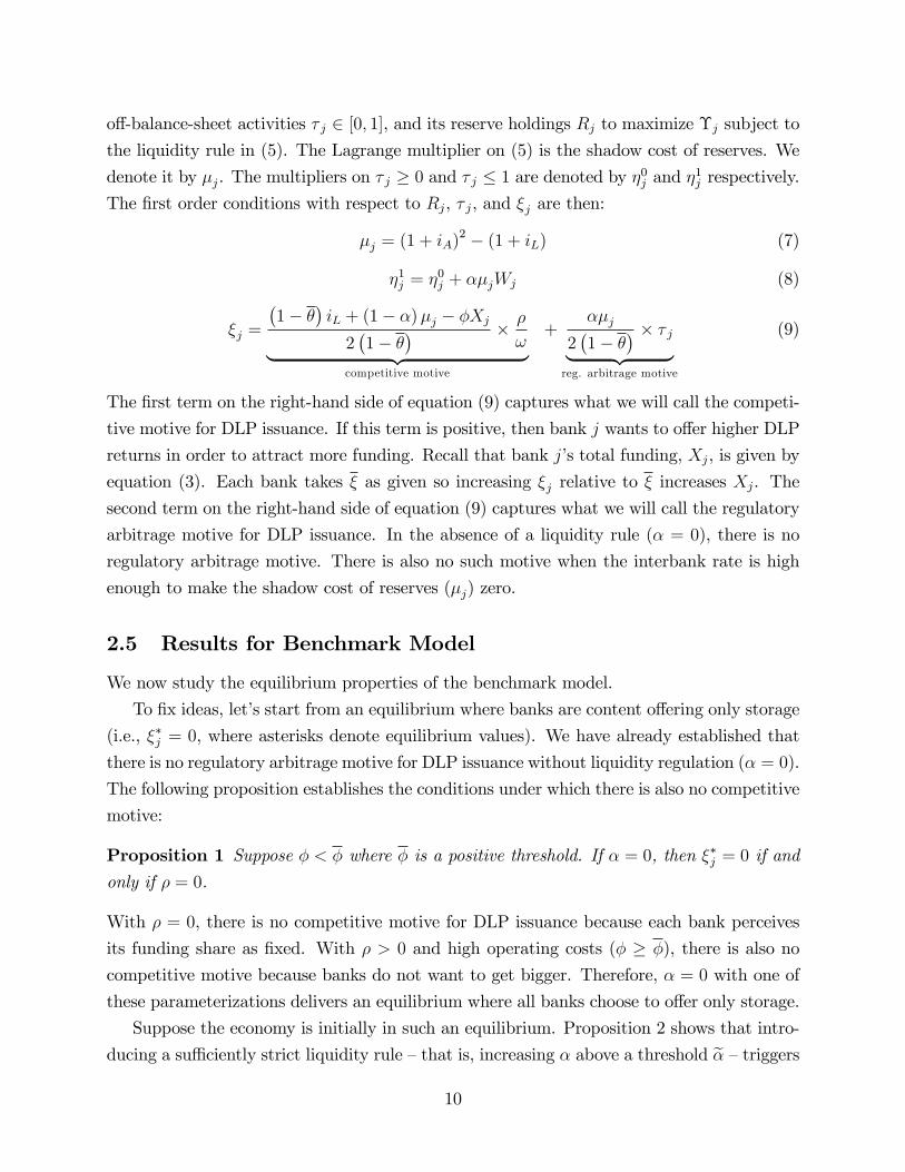
off-balance-sheet activities τ j ∈ [0, 1], and its reserve holdings Rj to maximize Υj subject to

the liquidity rule in (5). The Lagrange multiplier on (5) is the shadow cost of reserves. We

denote it by µj. The multipliers on τ j ≥ 0 and τ j ≤ 1 are denoted by η0j and η

1j respectively.

The first order conditions with respect to Rj, τ j, and ξj are then:

µj = (1 + iA)2 − (1 + iL) (7)

η1j = η0

j + αµjWj (8)

ξj =

(1− θ

)iL + (1− α)µj − φXj

2(1− θ

) × ρ

ω︸ ︷︷ ︸competitive motive

+αµj

2(1− θ

) × τ j︸ ︷︷ ︸reg. arbitrage motive

(9)

The first term on the right-hand side of equation (9) captures what we will call the competi-

tive motive for DLP issuance. If this term is positive, then bank j wants to offer higher DLP

returns in order to attract more funding. Recall that bank j’s total funding, Xj, is given by

equation (3). Each bank takes ξ as given so increasing ξj relative to ξ increases Xj. The

second term on the right-hand side of equation (9) captures what we will call the regulatory

arbitrage motive for DLP issuance. In the absence of a liquidity rule (α = 0), there is no

regulatory arbitrage motive. There is also no such motive when the interbank rate is high

enough to make the shadow cost of reserves (µj) zero.

2.5 Results for Benchmark Model

We now study the equilibrium properties of the benchmark model.

To fix ideas, let’s start from an equilibrium where banks are content offering only storage

(i.e., ξ∗j = 0, where asterisks denote equilibrium values). We have already established that

there is no regulatory arbitrage motive for DLP issuance without liquidity regulation (α = 0).

The following proposition establishes the conditions under which there is also no competitive

motive:

Proposition 1 Suppose φ < φ where φ is a positive threshold. If α = 0, then ξ∗j = 0 if and

only if ρ = 0.

With ρ = 0, there is no competitive motive for DLP issuance because each bank perceives

its funding share as fixed. With ρ > 0 and high operating costs (φ ≥ φ), there is also no

competitive motive because banks do not want to get bigger. Therefore, α = 0 with one of

these parameterizations delivers an equilibrium where all banks choose to offer only storage.

Suppose the economy is initially in such an equilibrium. Proposition 2 shows that intro-

ducing a suffi ciently strict liquidity rule —that is, increasing α above a threshold α —triggers

10

the issuance of off-balance-sheet DLPs. The benchmark model thus delivers a shadow bank-

ing sector:

Proposition 2 Suppose ρ = 0. There is a unique α ∈[0, θ)such that ξ∗j = 0 if α ≤ α and

ξ∗j > 0 with τ ∗j = 1 otherwise.

The incentive to issue DLPs in Proposition 2 does not come from competition since ρ = 0

eliminates the competitive motive. Instead, DLPs are issued because they can be booked

off-balance-sheet, away from the binding liquidity rule. It is straightforward to show that

ρ > 0 with φ suffi ciently high delivers the same intuition as Proposition 2.

Consider now the aggregate effects. Proposition 3 shows that introducing a liquidity

minimum into the benchmark model lowers the equilibrium interbank rate. It is then imme-

diate, given equation (4), that total credit (X −R∗j ) also falls.4 In other words, introducingregulation into the benchmark model with only small banks has the intended effect.

Proposition 3 For any ρ ≥ 0, the interbank rate in the benchmark model is highest at

α = 0. Therefore, moving from α = 0 to α > 0 will not increase the interbank rate or total

credit. Moving from α = 0 and ρ = 0 to α > 0 and ρ > 0 also will not increase the interbank

rate or total credit.

Proposition 3 is basically the market mechanism at work. Suppose there is no government

intervention (α = 0). At low interbank rates, price-taking banks will rely on the interbank

market for liquidity instead of holding their own reserves. In a Walrasian market, all banks

are price-takers so liquidity demand at t = 1 will exceed liquidity supply. This cannot be

an equilibrium. Therefore, the interbank rate must be high to substitute for government

intervention.5

3 Full Model: Heterogeneity in Market Power

We now extend the benchmark model to include a big bank. By definition of being big, this

bank will internalize how all of its choices affect the equilibrium.

We keep the continuum of small banks, j ∈ [0, 1], and index the big bank by k. DLP

demands are Wj = ωξj and Wk = ωξk, similar to equation (1). The funding attracted by

each bank is an augmented version of equation (3), namely:

Xj = 1− δ0 + (δ1 + δ2) ξj − δ1ξk − δ2ξj (10)

4With ψ = 0 in (4), total credit would be constant. Either way then, there cannot be a credit boom.5See Farhi, Golosov, and Tsyvinski (2009) for a different environment in which a liquidity floor decreases

interest rates.

11

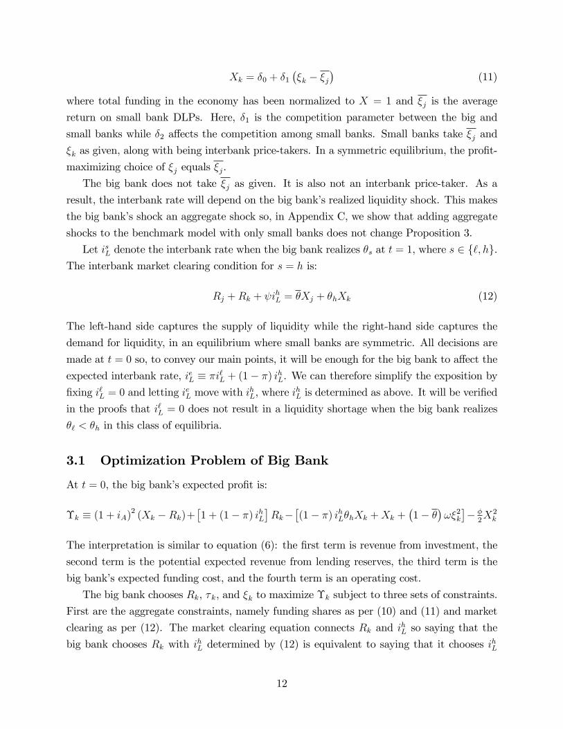
Xk = δ0 + δ1

(ξk − ξj

)(11)

where total funding in the economy has been normalized to X = 1 and ξj is the average

return on small bank DLPs. Here, δ1 is the competition parameter between the big and

small banks while δ2 affects the competition among small banks. Small banks take ξj and

ξk as given, along with being interbank price-takers. In a symmetric equilibrium, the profit-

maximizing choice of ξj equals ξj.

The big bank does not take ξj as given. It is also not an interbank price-taker. As a

result, the interbank rate will depend on the big bank’s realized liquidity shock. This makes

the big bank’s shock an aggregate shock so, in Appendix C, we show that adding aggregate

shocks to the benchmark model with only small banks does not change Proposition 3.

Let isL denote the interbank rate when the big bank realizes θs at t = 1, where s ∈ `, h.The interbank market clearing condition for s = h is:

Rj +Rk + ψihL = θXj + θhXk (12)

The left-hand side captures the supply of liquidity while the right-hand side captures the

demand for liquidity, in an equilibrium where small banks are symmetric. All decisions are

made at t = 0 so, to convey our main points, it will be enough for the big bank to affect the

expected interbank rate, ieL ≡ πi`L + (1− π) ihL. We can therefore simplify the exposition by

fixing i`L = 0 and letting ieL move with ihL, where i

hL is determined as above. It will be verified

in the proofs that i`L = 0 does not result in a liquidity shortage when the big bank realizes

θ` < θh in this class of equilibria.

3.1 Optimization Problem of Big Bank

At t = 0, the big bank’s expected profit is:

Υk ≡ (1 + iA)2 (Xk −Rk)+[1 + (1− π) ihL

]Rk−

[(1− π) ihLθhXk +Xk +

(1− θ

)ωξ2

k

]− φ

2X2k

The interpretation is similar to equation (6): the first term is revenue from investment, the

second term is the potential expected revenue from lending reserves, the third term is the

big bank’s expected funding cost, and the fourth term is an operating cost.

The big bank chooses Rk, τ k, and ξk to maximize Υk subject to three sets of constraints.

First are the aggregate constraints, namely funding shares as per (10) and (11) and market

clearing as per (12). The market clearing equation connects Rk and ihL so saying that the

big bank chooses Rk with ihL determined by (12) is equivalent to saying that it chooses ihL

12

with Rk determined by (12). This is the sense in which the big bank is a price-setter on the

interbank market.

The second set of constraints are the first order conditions of small banks. The repre-

sentative small bank solves essentially the same problem as before: its objective function is

still given by (6) but with (1− π) ihL as the interbank rate and Xj as per equation (10).

The last set of constraints on the big bank’s problem are inequality constraints, namely

the liquidity rule and non-negativity conditions:

Rk ≥ α (Xk − τ kWk)

τ k ∈ [0, 1]

ξk ≥ 0

µj ≥ 0

where µj is the shadow cost of reserves or, equivalently, the Lagrange multiplier on the

liquidity rule in the small bank problem. Each inequality constraint listed above can be

either binding or slack.

3.2 Results for Full Model

An equilibrium in the full model is characterized by the first order conditions from the small

bank problem, the first order conditions from the big bank problem, and interbank market

clearing.

Following Section 2.5, let’s start from an equilibrium where all banks offer only storage.

We know from our analysis of the benchmark model that small banks will have a competitive

motive for DLP issuance if (i) they do not perceive their funding shares as fixed and (ii)

operating costs are low enough that they want to expand. Notice that δ1 +δ2 > 0 in equation

(10) furnishes (i). If instead δ1 +δ2 = 0, then small banks take their funding shares as given6

and the first order conditions from their optimization problem deliver:

µj[Rj − α

(Xj − ωξj

)]= 0 with complementary slackness (13)

µj = (1 + iA)2 −[1 + (1− π) ihL

](14)

6With δ1+δ2 = 0, equation (10) becomes Xj = 1−δ0+δ1(ξj − ξk

). In a symmetric equilibrium, ξj = ξj

so there is still an indirect effect of ξj on Xj . The point is that small banks are not setting ξj to exploit thiseffect.

13

ξj =αµj

2(1− θ

) (15)

In words, these equations say that small banks are content offering only storage unless there

is a liquidity rule (α > 0) and a shadow cost to holding reserves (µj > 0). With α > 0 and

µj > 0, small banks would also offer off-balance-sheet DLPs, which is the same regulatory

arbitrage motive for DLP issuance seen in equations (8) and (9) of the benchmark model.7

Clearly, α = 0 will be enough to deliver an initial equilibrium without regulatory arbitrage

so that small banks do indeed offer only storage at the combination of α = 0 and δ1 +δ2 = 0.

To simplify the analytical exposition and develop clear intuition, this section will study

a move from α = 0 to α > 0 assuming δ1 + δ2 = 0. In Section 5.1, we will calibrate the

starting and ending values of α to data and allow δ1 + δ2 > 0. We will then calibrate an

operating cost parameter for small banks (φj) that is consistent with no DLP issuance in

the initial steady state.8

The property that the big bank also offers only storage when α = 0 can be delivered in

one of two ways as well. One approach is to set δ1 = 0 in equation (11) so that the big bank’s

funding share is fixed at Xk = δ0. Another approach is to keep the big bank’s funding share

endogenous (i.e., δ1 > 0) but set a suffi ciently high operating cost parameter which eliminates

any incentive for the big bank to increase its funding share (and hence issue DLPs) at the

configuration of parameters in the initial equilibrium. We will present analytical results for

both approaches to isolate how, if at all, an endogenous funding share affects the big bank’s

decision-making. When considering the second approach in the analytical results below, we

will set φ so that, in the initial equilibrium, ξk is exactly zero as opposed to being constrained

by zero. The numerical results in Section 5.1 will also follow the second approach, calibrating

φk for the big bank to distinguish it from the φj for small banks mentioned above.

Having explained the defining features of the initial equilibrium, let’s consider the dis-

tribution of reserves between big and small banks in this equilibrium. This was not a

consideration in the benchmark model because all banks were ex ante identical price-takers.

Now the big bank is a price-setter so its reserve choices may differ from that of small banks.

Proposition 4 Suppose α = 0. Consider δ1 + δ2 = 0 and either δ1 = 0 or δ1 > 0 with

φ suffi ciently positive so that the initial equilibrium has ξ∗j = ξ∗k = 0. If iA lies within an

intermediate range, then the initial equilibrium also involves µ∗j > 0, R∗j = 0, and R∗k > 0.

7See the proof of Proposition 2 for further discussion.8Notice that the approach in the calibration imposes weaker conditions than δ1+δ2 = 0: the latter means

that there is never a competitive motive among small banks while the former just means that there is nocompetitive motive at the parameters of the initial equilibrium. The main qualitative results do not dependon which approach is used.

14

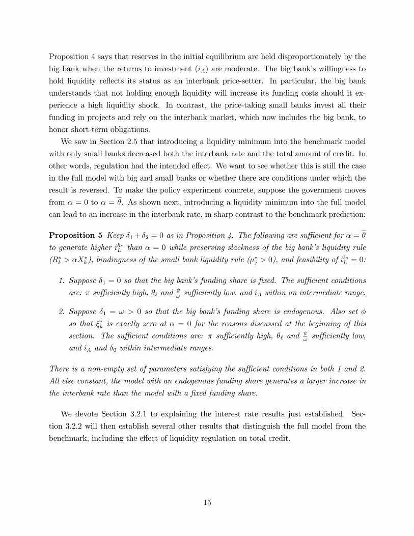
Proposition 4 says that reserves in the initial equilibrium are held disproportionately by the

big bank when the returns to investment (iA) are moderate. The big bank’s willingness to

hold liquidity reflects its status as an interbank price-setter. In particular, the big bank

understands that not holding enough liquidity will increase its funding costs should it ex-

perience a high liquidity shock. In contrast, the price-taking small banks invest all their

funding in projects and rely on the interbank market, which now includes the big bank, to

honor short-term obligations.

We saw in Section 2.5 that introducing a liquidity minimum into the benchmark model

with only small banks decreased both the interbank rate and the total amount of credit. In

other words, regulation had the intended effect. We want to see whether this is still the case

in the full model with big and small banks or whether there are conditions under which the

result is reversed. To make the policy experiment concrete, suppose the government moves

from α = 0 to α = θ. As shown next, introducing a liquidity minimum into the full model

can lead to an increase in the interbank rate, in sharp contrast to the benchmark prediction:

Proposition 5 Keep δ1 + δ2 = 0 as in Proposition 4. The following are suffi cient for α = θ

to generate higher ih∗L than α = 0 while preserving slackness of the big bank’s liquidity rule

(R∗k > αX∗k), bindingness of the small bank liquidity rule (µ∗j > 0), and feasibility of i`∗L = 0:

1. Suppose δ1 = 0 so that the big bank’s funding share is fixed. The suffi cient conditions

are: π suffi ciently high, θ` andψωsuffi ciently low, and iA within an intermediate range.

2. Suppose δ1 = ω > 0 so that the big bank’s funding share is endogenous. Also set φ

so that ξ∗k is exactly zero at α = 0 for the reasons discussed at the beginning of this

section. The suffi cient conditions are: π suffi ciently high, θ` andψωsuffi ciently low,

and iA and δ0 within intermediate ranges.

There is a non-empty set of parameters satisfying the suffi cient conditions in both 1 and 2.

All else constant, the model with an endogenous funding share generates a larger increase in

the interbank rate than the model with a fixed funding share.

We devote Section 3.2.1 to explaining the interest rate results just established. Sec-

tion 3.2.2 will then establish several other results that distinguish the full model from the

benchmark, including the effect of liquidity regulation on total credit.

15

3.2.1 Intuition for Interest Rate Response

To explain Proposition 5, it will be useful to summarize all the forces behind the big bank’s

choice of ihL. Differentiating the big bank’s objective function with respect to ihL:

∂Υk

∂ihL∝ Rk − θhXk︸ ︷︷ ︸

direct motive

−[

(1 + iA)2 − 1

1− π − ihL

]∂Rk

∂ihL︸ ︷︷ ︸reallocation motive

+

[(1 + iA)2 − 1− φXk

1− π − θhihL

]∂Xk

∂ihL︸ ︷︷ ︸funding share motive

(16)

The equilibrium ihL solves∂Υk∂ihL

= 0 when the relevant inequality constraints in the big bank’s

problem are slack. This is the appropriate case given the statement of Proposition 5. We

will start by explaining the three motives identified in (16). We will then explain how the

strength of each motive varies with α in order to understand why moving from α = 0 to

α = θ generates a higher interbank rate.

First is the direct motive. The big bank has reserves Rk and a funding share Xk. Its

net reserve position when hit by a high liquidity shock is therefore Rk − θhXk. Each unit

of reserves is valued at an interest rate of ihL when the big bank’s shock is high so, on the

margin, an increase in ihL changes the big bank’s profits by Rk − θhXk.

Second is the reallocation motive. The idea is that changes in ihL also affect how many

reserves the big bank needs to hold in a market clearing equilibrium. If ∂Rk∂ihL

< 0, then an

increase in ihL elicits enough liquidity from other sources to let the big bank reallocate funding

from reserves to investment. On the margin, the value of this reallocation is the shadow cost

of reserves, hence the coeffi cient on ∂Rk∂ihL

in (16).

Third is the funding share motive. The idea is that changes in ihL also affect how much

funding the big bank attracts when funding shares are endogenous. If ∂Xk∂ihL

> 0, then an

increase in ihL curtails the DLP offerings of small banks by enough to boost the big bank’s

funding share. The coeffi cient on ∂Xk∂ihL

in (16) captures the marginal value of a higher funding

share for the big bank. We will discuss this coeffi cient in more detail below.

To gain some insight into how changes in α will affect the solution to ∂Υk∂ihL

= 0 through

each motive, let’s start with the case of fixed funding shares (δ1 = 0). Consider first the

direct motive. Using the market clearing condition:

Rk − θhXkδ1=0= θ (1− δ0)− ψihL − α

(1− δ0 −

αω (1− π)

2(1− θ

) [(1 + iA)2 − 1

1− π − ihL

])︸ ︷︷ ︸

Rj as per small bank FOCs in (13) to (15)

(17)

For a given value of ihL, the magnitude of the direct motive in (17) depends on α through the

16

reserve holdings of small banks. There are two competing effects. On one hand, higher α

forces small banks to hold more reserves per unit of on-balance-sheet funding. On the other

hand, higher α can compel small banks to engage in regulatory arbitrage, decreasing their

on-balance-sheet funding as they offer off-balance-sheet DLPs (i.e., ξj > 0 with τ j = 1).

The net effect is ambiguous so we must look beyond the direct motive to fully understand

Proposition 5.

With fixed funding shares, the only other motive is the reallocation motive, where:

∂Rk

∂ihL

∣∣∣∣δ1=0

= −ψ − α2ω (1− π)

2(1− θ

) < 0 (18)

This expression is negative for two reasons. First and as captured by the first term in (18),

a higher interbank rate will attract more external liquidity, allowing the big bank to hold

fewer reserves. Second and as captured by the second term in (18), small banks will increase

their reserves when the interbank rate increases, also allowing the big bank to hold fewer

reserves. The effect of ihL on Rj that underlies the second term works through the regulatory

arbitrage motive of small banks: there is less incentive to circumvent a liquidity regulation

when the price of liquidity is expected to be high. We can also infer from the second term

that the effect of ihL on Rj strengthens with α. This is both because Rj is more responsive

to changes in ξj at high α (see equation (13)) and because ξj is more responsive to changes

in ihL at high α (see equations (14) and (15)).

This discussion helps explain the first bullet in Proposition 5: when funding shares are

fixed, high α makes it easier for the big bank to use high interbank rates to incent small

banks to share the burden of keeping the system liquid.

Does the same intuition extend to the case of endogenous funding shares? No because:

∂Rk

∂ihL

∣∣∣∣δ1=ω

= −ψ +αωπ (θh − θ`) (1− π)

2(1− θ

) (19)

An increase in ihL still decreases ξj but now a decrease in ξj also decreases how much funding

small banks attract (Xj) and therefore how many reserves they will want to hold.9 This

effect is strong enough to make the second term in (19) positive, in contrast to the second

term in (18).

We must therefore turn to the funding share motive to fully understand why introducing

a liquidity minimum can increase the equilibrium interbank rate when funding shares are

9See footnote 6 for the effect of ξj on Xj when δ1 + δ2 = 0.

17

endogenous. Recall the expression for the funding share motive from (16) and note:

∂Xk

∂ihL

∣∣∣∣δ1=ω

=αω (1− π)

2(1− θ

) > 0 (20)

We already know from the discussion of (19) that an increase in ihL decreases ξj which

then decreases the small bank funding share Xj. Total funding is normalized to one so the

decrease in Xj implies an increase in the big bank funding share Xk. The expression in (20)

is therefore positive. The magnitude of this expression increases with α because ξj is more

responsive to changes in ihL at high α (see equations (14) and (15)). It is therefore easier for

the big bank to increase its funding share by increasing ihL when α is high.

There is, of course, a difference between the ability to increase funding share and the

desire to do so. To complete the intuition, let us reconcile the big bank’s desire to increase

its funding share when α is high with the existence of convex operating costs. Return to

the coeffi cient on ∂Xk∂ihL

in (16). All else constant, moving from α = 0 to α = θ will trigger

regulatory arbitrage by small banks. The presence of ξj > 0 will then erode the big bank’s

funding share Xk, lowering its marginal operating cost φXk.

We can now understand the second bullet in Proposition 5 as follows: when funding

shares are endogenous, high α makes it easier for the big bank to use high interbank rates

to stop small banks from encroaching on its funding share. The last part of Proposition 5

establishes that sizeable increases in the interbank rate are most consistent with this sort of

asymmetric competition, wherein the big bank uses its interbank market power to fend off

competition from small banks and their off-balance-sheet activities.

3.2.2 Credit Boom and Cross-Sectional Predictions

We have now explained how the full model can deliver an increase in the equilibrium inter-

bank rate when a liquidity minimum is introduced. Proposition 6 below shows that the full

model also delivers an increase in total credit (1 − R∗j − R∗k) after the introduction of thisregulation. In other words, unlike the benchmark model, regulation in the full model can be

entirely counterproductive. Proposition 6 also summarizes the cross-sectional implications of

introducing liquidity regulation into the full model, namely convergence of on-balance-sheet

ratios and more aggressive issuance of DLPs by small banks relative to the big bank (i.e.,

ξ∗j > ξ∗k). Under the parameter conditions in Proposition 5, which are also the parameter

conditions in Proposition 6, the small bank liquidity rule is binding and the big bank liq-

uidity rule is slack. Therefore, small banks issue all their DLPs off-balance-sheet (τ ∗j = 1)

while the big bank is indifferent between any τ ∗k ∈ [0, 1]. We use τ ∗k = 0 in the proofs to

18

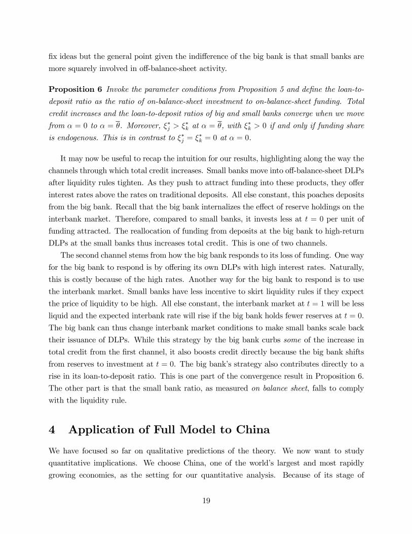
fix ideas but the general point given the indifference of the big bank is that small banks are

more squarely involved in off-balance-sheet activity.

Proposition 6 Invoke the parameter conditions from Proposition 5 and define the loan-to-

deposit ratio as the ratio of on-balance-sheet investment to on-balance-sheet funding. Total

credit increases and the loan-to-deposit ratios of big and small banks converge when we move

from α = 0 to α = θ. Moreover, ξ∗j > ξ∗k at α = θ, with ξ∗k > 0 if and only if funding share

is endogenous. This is in contrast to ξ∗j = ξ∗k = 0 at α = 0.

It may now be useful to recap the intuition for our results, highlighting along the way the

channels through which total credit increases. Small banks move into off-balance-sheet DLPs

after liquidity rules tighten. As they push to attract funding into these products, they offer

interest rates above the rates on traditional deposits. All else constant, this poaches deposits

from the big bank. Recall that the big bank internalizes the effect of reserve holdings on the

interbank market. Therefore, compared to small banks, it invests less at t = 0 per unit of

funding attracted. The reallocation of funding from deposits at the big bank to high-return

DLPs at the small banks thus increases total credit. This is one of two channels.

The second channel stems from how the big bank responds to its loss of funding. One way

for the big bank to respond is by offering its own DLPs with high interest rates. Naturally,

this is costly because of the high rates. Another way for the big bank to respond is to use

the interbank market. Small banks have less incentive to skirt liquidity rules if they expect

the price of liquidity to be high. All else constant, the interbank market at t = 1 will be less

liquid and the expected interbank rate will rise if the big bank holds fewer reserves at t = 0.

The big bank can thus change interbank market conditions to make small banks scale back

their issuance of DLPs. While this strategy by the big bank curbs some of the increase in

total credit from the first channel, it also boosts credit directly because the big bank shifts

from reserves to investment at t = 0. The big bank’s strategy also contributes directly to a

rise in its loan-to-deposit ratio. This is one part of the convergence result in Proposition 6.

The other part is that the small bank ratio, as measured on balance sheet, falls to comply

with the liquidity rule.

4 Application of Full Model to China

We have focused so far on qualitative predictions of the theory. We now want to study

quantitative implications. We choose China, one of the world’s largest and most rapidly

growing economies, as the setting for our quantitative analysis. Because of its stage of

19

development, China’s banking system has elements in common with both emerging and

advanced economies, making the lessons informative for a wider range of countries. Moreover,

China has experienced unprecedented growth in private credit relative to private savings over

the past decade. Our model predicts that some credit booms are caused by stricter liquidity

regulation so we are interested to know whether stricter liquidity regulation can account for

at least part of the Chinese experience.

Before proceeding to a full quantitative analysis in Section 5, we establish a mapping

from the model to China. Section 4.1 provides some institutional background on the Chinese

system and discusses the policies that amount to a tightening of liquidity regulation. We then

turn to the data. Propositions 5 and 6 showed that several other changes may accompany a

credit boom after stricter liquidity regulation. First is convergence of banks’on-balance-sheet

loan-to-deposit ratios, with large banks’ratios increasing and small banks’ratios decreasing.

Second is emergence of deposit-like products that offer elevated rates of return, with more

aggressive provision of such products by small banks than by large banks and much more

off-balance-sheet accounting of such products by small banks than by large banks. Third

is restrictive behavior on the interbank market by large banks along with a higher average

interbank interest rate and a larger gap between peak and trough interest rates. Section 4.2

documents the occurrence of the first phenomenon in China, Section 4.3 the second, and

Section 4.4 the third. Section 4.3 also presents direct evidence that small banks responded

to stricter liquidity regulation while large banks responded to the activities of small banks.

Our primary dataset is the Wind Financial Terminal. In cases where Wind is insuffi cient,

we collect data from bank annual reports, regulatory agencies, and financial association

websites.

4.1 Institutional Background

This section describes the basic features of China’s banking system and how they map into

our framework. We refer the reader to Appendix D for a more detailed discussion of the

reforms and regulations summarized here.

The Chinese economy is served by both big and small banks. Until the late 1970s, China

had a Soviet-style financial system where the central bank was the only bank. The Chinese

government moved away from this system in the late 1970s and early 1980s by establishing

four commercial banks (the Big Four). Market-oriented reforms initiated in the 1990s made

the Big Four much more profit-driven and opened the banking sector up to entry by small

and medium-sized commercial banks. China now has twelve joint-stock commercial banks

(JSCBs) operating nationally and over two hundred city banks operating in specific regions.

20

Many rural banks have also emerged. The JSCBs are typically larger than the city and rural

banks but all of these banks are still individually small when compared to the Big Four.

Although the Chinese government dramatically loosened its grip on the Big Four as part

of the market-oriented reforms, a legacy expectation of minimal competition between these

four banks remains. China’s banking sector can therefore be approximated by one big bank

and many small banks. This maps into the environment of our full model.

Further reform by the government in 2005 expanded the range of financial services banks

could provide. This led to the advent of wealth management products or WMPs for short.

WMPs are well approximated by the DLPs in our model. In particular, WMPs represent

a liquidity service provided by banks at endogenous interest rates. Banks can also choose

where to report their WMPs by choosing whether or not to provide an explicit principal

guarantee. Any WMPs issued with an explicit principal guarantee must be reported on-

balance-sheet. Absent such a guarantee, the WMP and the assets it invests in do not have

to be consolidated into the bank’s balance sheet. These unconsolidated WMPs are invested

off-balance-sheet, typically with the help of a lightly-regulated financial institution called a

trust company. A more detailed discussion of trust companies and their involvement with

WMPs appears in Appendix D. The lack of explicit guarantees on off-balance-sheet WMPs

is only for accounting purposes though: there is a general perception that all WMPs are at

least implicitly guaranteed by traditional banks (see also Elliott, Kroeber, and Qiao (2015)).

Turning to the regulatory environment, China’s banks are currently regulated by the

People’s Bank of China (central bank) and the China Banking Regulatory Commission

(CBRC). A loan-to-deposit cap was introduced in 1995 to prevent banks from lending more

than 75% of the value of their deposits to non-financial borrowers. However, enforcement

was lax until 2008 when CBRC moved to curb lending and bolster liquidity, particularly at

small and medium-sized banks.10 CBRC began by policing the end-of-year loan-to-deposit

ratios of all banks more carefully. It then switched to end-of-quarter ratios in late 2009,

end-of-month ratios in late 2010, and average daily ratios in mid-2011. Our sample ends

in 2014, at which point CBRC was still monitoring average daily ratios. The 2008-2014

period in China thus involved stricter liquidity regulation than the years just prior. Stricter

enforcement of the loan-to-deposit cap by CBRC during this period was also complemented

by a rapid increase in the reserve requirements set by the central bank.

Banks in China are also subject to capital requirements and deposit rate regulation. Cap-

ital requirements follow the international Basel Accords and were a non-binding constraint

on Chinese banks for the period of interest. Deposit rate regulations involved the central

10As we will establish in Section 4.2, these banks had higher loan-to-deposit ratios than the Big Four,consistent with the predictions of our model.

21

bank essentially setting deposit rates until late 2015. Our model allows for a liquidity ser-

vice with exogenous interest rates. Recall that we have storage with iB = iD = 0. In the

calibration, we can upgrade storage to a traditional deposit which has iB > 0 and iD > 0 as

set by the government. DLPs, if offered in equilibrium, will pay an additional return relative

to these positive rates. Deposit rate regulation in China only applies to traditional deposits

so, like the DLPs in our model, WMPs have endogenously determined interest rates.

4.2 Convergence of Loan-to-Deposit Ratios

Figure 1 plots on-balance-sheet loan-to-deposit ratios for the Big Four and the JSCBs from

2005 to 2014.11 There are three major takeaways. First, the JSCBs have historically had

higher loan-to-deposit ratios than the Big Four, as predicted by the theory.12 Second, stricter

enforcement of a 75% loan-to-deposit cap starting around 2008 constrains the JSCBs but not

the Big Four. This is observed most clearly by looking at ratios based on average balances

during the year rather than end-of-year balances. As a group, the JSCBs were just satisfying

the 75% cap in terms of end-of-year loan-to-deposit ratios when stricter enforcement began.

However, using average balances during the year, the JSCBs had loan-to-deposit ratios which

well exceeded the 75% cap. This implies that the end-of-year ratios were window-dressed to

hit 75% and thus not reflective of the true position of the JSCBs. The enforcement action

that began in 2008 sought to impose a 75% cap on the true position of banks so it is in

this sense that CBRC imposed a binding constraint on the JSCBs. As CBRC increased

its monitoring frequency between 2008 and 2011, the difference between the end-of-year

and average balance ratios for JSCBs began to disappear. Also notice that the average

balance ratio of the JSCBs reached exactly 75% in 2012, the first full year of average balance

monitoring by CBRC. In contrast, there has never been a sizeable difference between the

average balance and end-of-year ratios of the Big Four, with both ratios comfortably below

75% when stricter enforcement began.13

The third major takeaway from Figure 1 is that the loan-to-deposit ratio of the Big Four

has increased towards 75% since the beginning of the enforcement. This increase reflects

both higher loan growth and lower deposit growth relative to the pre-enforcement period.

11Historical balance sheet data for city and rural banks is spotty, particularly when it comes to averagedaily balances, so these banks are excluded from the figure.12On this point, small banks in the U.S. have historically also had higher loan-to-deposit ratios than large

banks. For example, among nationally chartered banks in the U.S., the difference averages 9 percentagepoints over the period 1985 to 2000, with small and large banks as defined in FRED data.13A common narrative is that the Chinese government uses individual loan quotas to impose even stricter

limits on big banks. In practice though, individual loan quotas in China are negotiable, particularly for theBig Four who have more bargaining power than the JSCBs and the city/rural banks, so the Big Four shouldstill be viewed as choosing their own loan-to-deposit ratios.

22

From 2005 to 2008, loans and deposits at the Big Four grew at annualized rates of 10.9%

and 14.1% respectively. From 2008 to 2014, these rates were 16.7% and 12.3% respectively.

China’s State Council announced a two-year stimulus package in late 2008 which would have

required the banking sector to fund roughly RMB 4 trillion of new investment. Appendix E

uses a money multiplier calculation to purge loan and deposit growth of the effects of this

package. We find that loans and deposits at the Big Four would have grown at annualized

rates of 12.9% and 9.8% respectively from 2008 to 2014 absent the stimulus package. The

Big Four loan-to-deposit ratio would have then increased from 0.57 in 2008 to 0.67 in 2014.

This is around three-quarters of the actual increase plotted in Figure 1 so big banks in

China have become less liquid even taking into account the stimulus package. The period

of stricter loan-to-deposit enforcement was therefore accompanied by convergence of the on-

balance-sheet loan-to-deposit ratios of big and small banks, with the JSCB ratio decreasing

to comply with CBRC’s tougher stance and the Big Four ratio increasing beyond what can

be explained by stimulus. That such convergence would occur after enforcement imposed a

binding constraint on only small banks is as predicted in Proposition 6.

4.3 Evidence from Wealth Management Products

The theory also predicts emergence of deposit-like products with higher interest rates than

traditional deposits after a loan-to-deposit cap that binds on only small banks is enforced.

Moreover, small banks are predicted to offer higher interest rates on these products than

large banks and off-balance-sheet issuance is predicted to be dominated by small banks. We

start this section by showing these patterns in the data. We then present empirical evidence

on the mechanisms behind these patterns. Recently, a few other papers have also begun

using disaggregated data to comment on off-balance-sheet activities in China. We discuss

these papers in Appendix D and explain why we believe their results support our conclusions.

4.3.1 Patterns in WMP Issuance

Figure 2 plots the evolution of WMPs in China after these products became legal in 2005.

Notice that WMP activity was modest prior to 2008, with WMPs outstanding amounting to

less than 2% of GDP in 2006 and 2007. In contrast, the period after 2008 was characterized

by rapid growth of WMPs and, by 2014, the amount outstanding stood at nearly 25% of

GDP. The spread between annualized returns on 3-month WMPs and the 3-month deposit

rate has averaged 1 percentage point since 2008 and nearly 2 percentage points since 2012,

with virtually all WMPs delivering above or equal to their promised returns regardless of

whether or not an explicit principal guarantee was in place. Similar patterns are observed

23

at other maturities but we highlight 3-month rates since median WMP maturity has been

between 2 and 4 months since 2008.

Turning to the cross-section, the Big Four have indeed been less aggressive in WMP

issuance than small banks (i.e., JSCBs and smaller). From 2008 to 2014, the realized returns

on 3-month WMPs issued by small banks averaged over 30 basis points above the realized

returns on 3-month WMPs issued by banks in the Big Four. Moreover, the lowerbounds

promised by small banks averaged over 80 basis points above those promised by the Big

Four and, by 2014, the average lowerbound promised by small banks was 1.5 times the

average lowerbound promised by the Big Four.

The Big Four have also been less involved in booking WMPs off-balance-sheet, as pre-

dicted above. Between 2008 and 2014, small banks accounted for 73% of all new WMP

batches and issued 57% of their batches without a guarantee while the Big Four issued only

46% of their batches in this way. The gap in non-guaranteed intensity widens in the second

half of the sample, with small banks at 62% and the Big Four at 43%. These estimates are

based on product counts since Wind does not yet have complete data on the total funds

raised by each product. However, using data from CBRC and the annual reports of the

Big Four, we estimate that small banks accounted for roughly 64% of non-guaranteed WMP

balances outstanding at the end of 2013.14

In the model, the patterns just discussed arise because small banks are responding to

stricter enforcement of loan-to-deposit rules while big banks are responding to increased

competition from small banks. We now provide evidence on these mechanisms, beyond just

the patterns the model predicts they generate.

4.3.2 Small Banks Respond to Loan-to-Deposit Rules

A detailed case study will help identify the motives that drive small banks. We consider

China Merchants Bank (CMB), one of the twelve JSCBs. Between 2007 and 2013, CMB’s

loan-to-deposit ratio averaged 82% when calculated using average balances during the year.

This is in contrast to 74% when end-of-year balances are used. WMP issuance by CMB

increased from RMB 0.1 trillion in 2007 to RMB 0.7 trillion in 2008 before reaching almost

RMB 5 trillion in 2013. CMB accounted for only 3% of total banking assets in 2012 but

5.2% of WMPs outstanding at year-end and 17.7% of all WMPs issued during the year.15

14The entire WMP balance in Bank of China’s annual report is described as an unconsolidated balanceyet the micro data in Wind includes several guaranteed batches for this bank that would not have maturedby the end of 2013. We therefore remove Bank of China and rescale the other banks in the Big Four to backout our 64% estimate for small banks.15Based on data from KPMG, CBRC, and China Merchants Bank.

24

At the end of both 2012 and 2013, CMB had about 83% of its outstanding WMP balances

booked off-balance-sheet and, based on notes to the financial statements, figures for earlier

years were at least as high.

We argue that time variation in the maturity of CMB’s off-balance-sheet WMPs reveals

the importance of loan-to-deposit regulation for the evolution of these products. Figure 3

shows a sizeable drop in the median maturity of CMB’s off-balance-sheet products, from just

over 4 months in late 2009 to just under 1 month by mid-2011. This drop does not occur

for on-balance-sheet WMPs nor is it matched by a drop in the promised annualized yield on

off-balance-sheet products. Instead, the drop in CMB’s off-balance-sheet maturity coincides

with changes in CBRC’s monitoring of loan-to-deposit ratios. Recall from Section 4.1 that

CBRC focused on the end-of-year ratio until late 2009, the end-of-quarter ratio until late

2010, and the end-of-month ratio until mid-2011. CMB thus shortened the maturity of its

off-balance-sheet products as the frequency of CBRC exams increased.

This is significant because shorter maturities can be used to thwart more frequent end-

of-period exams. Upon maturity, the principal and interest from an off-balance-sheet WMP

are automatically transferred to the buyer’s deposit account. A buyer who wants to roll over

his investment then contacts his bank to have the transfer reversed. In the time between

the transfer and the reversal though, reserves and deposits rise, lowering the loan-to-deposit

ratio observed by CBRC.16 In the first half of 2011, CMB’s off-balance-sheet products had

a median maturity of just under 1 month which enables the window-dressing that thwarts

the end-of-month exams. To make this point more concrete, we look at the maturity of each

off-balance-sheet batch relative to its issue date. Approximately 15% of the off-balance-sheet

batches issued by CMB between January 2008 and December 2010 would have matured near

a month-end. This fraction jumped to 40% in early 2011.

Shortening the maturity of off-balance-sheet WMPs in response to increasingly frequent

monitoring of end-of-period loan-to-deposit ratios became futile in mid-2011 as CBRC began

monitoring average daily ratios, not end-of-period ratios. Accordingly, Figure 3 shows that

16Keeping the automatic deposits as reserves is one approach. Another is to bring loans back on balancesheet in the form of securities which derive their cash flows from the loans. The data suggest that CMB justrecorded reserves between 2009 and 2011. The process being discussed here —designing unguaranteed WMPsto automatically deposit before a regulatory check and recording a non-loan as the balancing asset —alsosheds light on how the JSCBs window-dressed their end-of-year balance sheets in Figure 1. Of course, thisprocess only sheds light on the post-2008 period when WMP issuance was non-trivial. A common practicepre-2008 was to call loans shortly before a potential inspection (e.g., the end of a calendar year). The bankpromises to re-issue these loans within a few weeks and, in the intervening time, borrowers whose loans werecalled essentially rely on loan sharks. This practice is only feasible if it does not have to occur frequently(i.e., the borrowers cannot afford to rely increasingly on loan sharks). Therefore, in the era of stricter andmore frequent loan-to-deposit enforcement, any end-of-period window-dressing was primarily accomplishedvia the maturity of unguaranteed WMPs.

25

CMB’s median off-balance-sheet maturity has returned to roughly 3 months. The fraction

of off-balance-sheet batches set to mature near a month-end has also fallen back below 20%.

Similar patterns are not observed for the Big Four. That is, changes in WMP maturity do

not track changes in CBRC’s monitoring of loan-to-deposit rules when we restrict attention

to WMPs issued by banks in the Big Four.

4.3.3 Big Banks Respond to Small Banks

Granger causality tests on WMP issuance in China show that big banks were responding to

small banks. Using monthly detrended data on WMP batches between January 2007 and

September 2014, the null hypothesis that WMP issuance by small banks does not Granger-

cause WMP issuance by the Big Four is rejected at 1% significance, regardless of the de-

trending method or the number of lags. The opposite hypothesis that WMP issuance by

the Big Four does not Granger-cause WMP issuance by the small banks cannot be rejected

at 10% significance. Our baseline specification is a VAR with six lags and detrending via

HP filter. The p-value for the null hypothesis that small bank issuance does not cause Big

Four issuance is 0.002 (χ2 statistic 21.104). In contrast, the p-value for the null that Big

Four issuance does not cause small bank issuance is 0.478 (χ2 statistic 5.5264). Changing

the number of lags can decrease the p-value on the latter null, but not below 0.1. Therefore,

the impetus for WMPs in China is indeed coming from small banks.

4.4 Interbank Conditions and Big Four Involvement

The last set of theoretical predictions to evaluate are about the interbank market. Propo-

sitions 5 and 6 showed that loan-to-deposit caps can lead to tighter interbank conditions

together with a credit boom. Big banks were an important force behind this result: in

the benchmark model with only small banks, the introduction of loan-to-deposit regulation

always led to a lower interbank interest rate and less credit.

Figure 4 shows that tighter and more volatile interbank markets have indeed accompanied

the period of interest. China has both an uncollateralized money market (solid black line)

and an interbank repo market (solid gray line). We will focus on the latter since it is much

larger than the former. However, both markets have clearly exhibited an upward trend in

interest rates since 2009 despite fairly large monetary injections by China’s central bank

(dashed red line). In the interbank repo market, the average interest rate weighted by

transaction volume was 50 basis points higher in 2014 than it was in 2007. The highest

weighted average rate observed in daily data also increased by 150 basis points after 2007,

reaching an unprecedented 11.6% in mid-2013.

26

We now want to evaluate the extent to which the Big Four contributed to the increase

in interbank rates. The incentives that push big banks to optimally tighten the interbank

market in our model need not generate a constantly higher interbank rate: an increase in the

average interbank rate is enough to increase small banks’incentives to hold liquidity. The

mid-2013 event was certainly relevant in this regard so we obtained transaction-level data

from the interbank repo market to study it in detail.

A common narrative in China is that interbank conditions tightened in mid-2013 be-

cause the government wanted to discipline the market (e.g., Elliott, Kroeber, and Qiao

(2015)). Banks in general experienced some liquidity pressure in early June 2013 as compa-

nies withdrew deposits to pay taxes and households withdrew ahead of a statutory holiday.17

Accordingly, the weighted average interbank repo rate rose from 4.6% on June 3 to 9.3%

on June 8 before falling back down to 5.4% on June 17. Most of the seasonal pressures

seemed to have subsided yet interbank rates rose again on June 20 after the government

indicated it would not inject extra liquidity. The weighted average repo rate hit 11.6%, with

minimum and maximum rates of 4.1% and 30% respectively. For comparison, the minimum

and maximum rates on June 3 were 3.9% and 5.3% respectively.

An analysis of individual transactions will show whether or not tightness on June 20 was

triggered by the government. Our identification strategy makes use of the fact that China

has three policy banks which raise money in bond markets to fund economic development

projects approved by the central government. The policy banks are not commercial banks

and are thus distinct from the Big Four, the JSCBs, and the city/rural banks. Wind data on

daily net positions from mid-2009 to mid-2010 reveals that the policy banks were the second

largest liquidity providers on the interbank market, second only to the Big Four.18 The policy

banks are essentially agents of the government whereas the Big Four have become much more

independent since the market-oriented reforms discussed in Section 4.1. Therefore, if the

interbank market tightened in mid-2013 at the hands of the government, the policy banks

should have been at least as restrictive as the Big Four.

The transaction-level data show that this was not the case. The policy banks provided

a lot of liquidity to the interbank market at fairly low interest rates, to the point that they

became the largest net lenders on June 20, 2013. The Big Four, on the other hand, were

extremely restrictive, amassing RMB 50 billion of net borrowing by the end of the trading

17The Economist, “The Shibor Shock,”June 22, 2013.18The Wind sample runs from July 2009 to September 2010 for a total of 309 trading days. On the 285

trading days where big banks and policy banks were both net lenders, big banks were the main net lender93% of the time. Moreover, when big banks were the main net lender, their net lending was 4.2 times thatof policy banks. In contrast, when policy banks were the main net lender, their net lending was only 1.6times that of big banks.

27

day. Figure 5 illustrates the sharp difference between the Big Four and the policy banks in

terms of both quantity and price of liquidity provision on June 20. The top panel illustrates

the reluctance of the Big Four to lend while the bottom panel illustrates a sizeable increase

in policy bank loans and the more moderate nature of policy bank interest rates.

The bottom panel of Figure 5 also reveals that much of the increase in policy bank

lending on June 20 was absorbed by the Big Four. Were big banks borrowing because they

really needed liquidity? Two pieces of evidence suggest no. First, the Big Four’s ratio of repo

lending to repo borrowing was 0.7, with 71% of the loans directed towards small banks. If the

Big Four were in dire need of liquidity on June 20, we would expect to see very little outflow.

Second, the repo activities of big banks involved a maturity mismatch. Overnight trades

accounted for 96% of big bank borrowing but only 83% of big bank lending to small banks.

Roughly 80% of policy bank lending to small banks was also at the overnight maturity. If

big banks really needed liquidity on June 20, we would expect the maturity of their lending

to be closer to the maturity of their borrowing. Instead, it was closer to the maturity offered

by policy banks to borrower groups that policy banks and big banks had in common.

Figure 6 shows that big banks also commanded an abnormally high interest rate spread

on June 20. In particular, their weighted average lending rate was 266 basis points above

their weighted average borrowing rate. This is high relative to other banks: JSCBs and city

banks commanded spreads of 113 and 46 basis points respectively. It is also high relative

to other days in the sample: on any other day in June 2013, the spread commanded by big

banks was between -40 and 58 basis points. Pricing among big banks was also much more

uniform than pricing among small banks, both on June 20 and throughout our sample. To

this point, we calculate the coeffi cient of variation (CV) of overnight lending rates offered by

banks in different groups and find that the CV among big banks was 61% of the CV among

JSCBs and 21% of the CV among city banks on June 20. Averaging over all trading days

in June 2013 yields similar figures, namely 62% and 29% respectively.19

Taken together, the evidence presented in this section indicates that big banks absorbed

policy bank liquidity and intermediated it to small banks at much higher interest rates. As

shown in Figure 7, JSCBs paid a lot more for non-policy bank loans on June 20 than they

did for policy bank loans. It then stands to reason that JSCBs would have liked a higher

share of policy bank lending. Instead, they received 20% of what policy banks lent on June

20, down from an average of 28% over the rest of the month.20 The situation was similar for

19We exclude lending rates charged to policy banks given the proximity of policy banks to the government.20For completeness, the overnight and 7 day maturities shown in Figure 7 were almost 94% of JSCB

borrowing on June 20. They were also 100% of JSCB borrowing from policy banks on this date. There wereno major differences in the haircuts imposed by policy banks versus other lenders.

28

city and rural banks: they faced large price differentials between policy and non-policy bank

loans yet their share of policy bank lending on June 20 was 22%, well below an average of

47% over the rest of the month.

In sum, the Big Four can and do change interbank conditions to the detriment of their

smaller competitors. Figure 4 showed a tightening of the interbank market over the same

period as the credit boom that we turn to next. This tightening occurred despite increasing

monetary injections by the central bank and our analysis of the most dramatic rise in inter-

bank rates revealed the Big Four as the driving force. All of these findings line up with the

theory.

5 Quantitative Analysis

We are now ready to quantify how much of China’s credit boom can be generated by stricter

liquidity regulation. We first present the calibration results. We then establish the external

validity of the calibrated model and use it to decompose the importance of various shocks.

5.1 Calibration Results

The starting point for our calibration is 2007, just prior to China’s adoption of stricter

liquidity rules. The ending point is 2014. The initial liquidity rule is set to α = 0.14 to

match the observed loan-to-deposit ratio of JSCBs in 2007. We use the ratio based on

average balances rather than end-of-year balances, as per Figure 1. The policy experiment

is then an increase from α = 0.14 to α = 0.25, capturing CBRC’s stricter enforcement of the

75% loan-to-deposit cap.

We take the time from t = 0 to t = 2 to be a quarter. All interest rates are quoted

on an annualized basis. We set (1 + iD)2 = 1.026 to match the average benchmark interest

rate of 2.6% for 3-month deposits in China. We set (1 + iB)2 = 1.004 to match the average

benchmark interest rate of 0.4% for demand deposits. The central bank’s benchmark interest

rate for loans with a maturity of less than six months averages 5.6%. We set (1 + iA)2 = 1.05

since banks can offer a discount of up to 10% on the benchmark loan rate.21

For the low liquidity shock, Proposition 5 points to a small magnitude (θ`) and a high

probability (π) so we use θ` = 0 and π = 0.75. The parameter conditions in Proposition 5 are

relevant for China given the strong empirical support found in Section 4 for the predictions

21We are assuming the same return iA for all banks. In practice, different banks can invest in differentsectors but the “risk-adjusted”returns are roughly comparable: while the private sector is more productivethan the state sector, lending to the private sector is, at least politically, riskier. Some anecdotal evidencecan be found in Dobson and Kashyap (2006).

29

of Propositions 5 and 6. Proposition 5 also points to a low external liquidity parameter (ψ)

so we use ψ = 0.5. In words, a one percentage point increase in the interbank rate prompts

a monetary injection by the central bank of 0.5% of total savings. This is a reasonable

magnitude in light of the data in Figure 4 for the period where the central bank injected

liquidity. We will allow i`L = iB > 0 in the calibration since surplus reserves can earn a

small interest rate from the central bank. We then redefine Ψ (iL) ≡ ψ (iL − iB) to preserve

Ψ(i`L)

= 0. The Big Four accounted for around 55% of all deposits in China in 2007 so we

also set δ0 = 0.55.

To calibrate the remaining parameters, we target moments in 2014. We can then use the

model to predict the 2007 values of these moments along with the credit-to-savings ratio in

2007 and 2014. The competition parameters (δ1 and δ2) and the WMP demand parameter

(ω) are calibrated to match funding outcomes in 2014. As per Figure 2, WMPs were around

25% of GDP at the end of 2014. This is equivalent to 15% of total savings. Small banks

accounted for roughly two-thirds of WMPs so we will target Wj = 0.10 and Wk = 0.05 for

2014. We will also target a funding share of Xk = 0.45 for 2014 since the Big Four accounted

for roughly 45% of all savings (i.e., traditional deposits plus WMPs) in that year.

We allow big and small banks to have different operating cost parameters, φk and φj.

China has around 200 commercial banks so a big bank is on average 40 times as large as

a small bank (i.e., 0.454/0.55

196). In the context of our model, this size difference implies that

the big bank faces φk below φj. To match the observed size difference, we set φj = 40φk so

that marginal operating costs are the same across banks.22 We then calibrate φk to match

a loan-to-deposit ratio of 0.70 for the Big Four in 2014. We will check that the resulting

operating cost parameters are high enough to deliver negligible WMP issuance in 2007.

Lastly, we calibrate the average liquidity shock, θ ≡ πθ` + (1− π) θh, to get an average

interbank rate of 3.6% when α = 0.25. The 3.6% target is the weighted average seven-day

interbank repo rate in 2014. The seven-day rate is the longest maturity for which there

is significant trading volume. It is diffi cult to target shorter-term (e.g., overnight) repo

rates since we are working with a two-period model and each period must be long enough to

match reasonable data on loan returns (iA). This is just a level effect though: the correlation

between the overnight and seven-day repo rates is around 0.95.

The results are summarized in Table 1.23 Our model generates most of the rise in WMPs

between 2007 and 2014. It also generates half of the increase in the average seven-day

22Differences in φ can be interpreted as differences in retail networks that stem from exogenous social orpolitical forces. In robustness checks, we found that cutting the

φjφkratio to five (based on the size difference

between the Big Four and only the JSCBs) and re-calibrating the model generates very similar results.23The calibrated parameters are: ω = 126.84, δ1 = 266.36, δ2 = 0.374, φk = 0.0335, and θ = 0.1325.

30

interbank repo rate. Since yearly averages can mask some of the most severe events, it is also

useful to consider the peak interbank rates observed before and after CBRC’s enforcement

action (10.1% and 11.6% respectively, as measured by daily averages). Of this 150 basis point

increase in peak rates, our model delivers 90 basis points. Returning to Table 1, the model

also delivers more than half of the decrease in the Big Four’s funding share. We also obtain

a large increase in the Big Four’s loan-to-deposit ratio, although the increase is somewhat

larger than what we observe in the data. Finally, we obtain a sizeable 3.2 percentage point

increase in the aggregate credit-to-savings ratio.

How does a 3.2 percentage point increase compare to China’s overall credit boom? Com-

mercial banks for which Bankscope has complete data collectively added RMB 40 trillion of

new loans between 2007 and 2014, pushing the ratio of traditional lending to GDP from 75%

in 2007 to 95% in 2014. We also know from Figure 2 that WMPs outstanding ballooned from

2% of GDP in 2007 to nearly 25% of GDP in 2014. CBRC estimates that roughly two-thirds

of WMP balances in 2012 and 2013 were non-guaranteed and hence off-balance-sheet. We

thus estimate that China’s shadow banking system grew from a negligible fraction of GDP in

2007 to 16% of GDP in 2014. Appendix D shows that our estimate of the growth of shadow

banking in China based on off-balance-sheet WMPs accounts for the majority of the growth

in broader measures of shadow banking that can be constructed using data from China’s

National Bureau of Statistics. Adding the growth of the traditional and shadow sectors, we

get a 35 percentage point increase in the ratio of total credit to GDP. This translates into

a roughly 10 percentage point increase in China’s credit-to-savings ratio, from 65% in 2007

to 75% in 2014. Appendix E shows that the RMB 4 trillion fiscal stimulus package under-

taken in 2009 and 2010 explains around 40% of this 10 percentage point increase. Therefore,

our model generates one-third of China’s overall credit boom and over one-half of what is

unexplained by the government’s stimulus package.

5.2 External Validation

We now examine the external validity of the calibrated model by checking whether it can

match empirical moments not targeted in the calibration, namely observed correlations be-

tween the interbank rate and the returns to WMPs issued by small and big banks. Table

2 reports these correlations, calculated using monthly data from January 2008 to December

2014. The time series for iL is the average interbank repo rate weighted by transaction

volume. The time series for ξj and ξk are the average returns promised by small and big

banks respectively on 3-month WMPs. Since Wind has only partial data on the amount of

funding raised by each WMP, ξj and ξk are unweighted averages. We will introduce error

31

terms to absorb imperfections in the measurement of ξj and ξk.

Table 2 shows that iL is positively correlated with each of ξj, ξk, and ξj−ξk. It also showsthat ξj is positively correlated with each of ξk and ξj − ξk while the correlation between ξkand ξj − ξk is not significant. We would like to know the extent to which our calibrated

model can replicate these correlations. To this end, we allow α, the parameter governing

liquidity regulation, to be drawn from a normal distribution:

α = α + εα (21)

where εα is normally distributed with mean 0 and variance σ2α. We set α = 0.14+0.25

2=

0.195, where α = 0.14 generated the initial loan-to-deposit ratio of 86% for small banks

in Section 5.1 and α = 0.25 generated the regulated ratio of 75%. We draw values of α

using equation (21) and simulate the model for each value to generate the average interbank

rate, πi`L + (1− π) ihL, the WMP returns offered by small banks, ξj + εξj , and the WMP

returns offered by big banks, ξk + εξk . Here, εξj and εξk denote measurement errors which

are drawn from two independent normal distributions with mean 0 and variances σ2ξjand σ2

ξk

respectively.24 We then use Simulated Method of Moments to estimate the three unknown

parameters σα, σξj , and σξk . Appendix F describes the estimation procedure in more detail.

The first column of Table 3 reports the estimated parameter values (Panel A) and pre-

dicted correlations (Panel B). The observed correlations from Table 2 appear in the last

column of Panel B. Notice that σα is quantitatively large and highly significant. Also no-

tice that the estimated model matches very well the observed correlations between iL and

each of ξj, ξk, and ξj − ξk. Shocks to α are therefore important for generating the right

correlations between the interbank rate and WMP returns. At the same time though, the

estimated model matches less well the pairwise correlations among WMP returns. It will

thus be useful to also allow for other shocks, as is done next.

5.3 Analysis of Other Shocks

We consider two other shocks: demand shocks and money supply shocks. We repeat the

exercise conducted in the first column of Table 3 for each of these shocks separately. We

then consider a version of the quantitative model which has demand shocks, money supply

shocks, and shocks to liquidity regulation at the same time.

24All distributions are truncated to avoid abnormal values of α, ξj , and ξk.

32

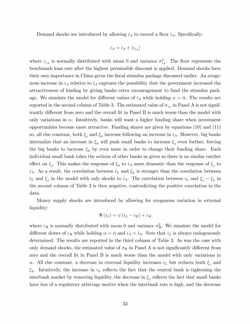
Demand shocks are introduced by allowing iA to exceed a floor ıA. Specifically:

iA = ıA + |εiA|

where εiA is normally distributed with mean 0 and variance σ2iA. The floor represents the

benchmark loan rate after the highest permissible discount is applied. Demand shocks have

their own importance in China given the fiscal stimulus package discussed earlier. An exoge-

nous increase in iA relative to ıA captures the possibility that the government increased the

attractiveness of lending by giving banks extra encouragement to fund the stimulus pack-

age. We simulate the model for different values of iA while holding α = α. The results are

reported in the second column of Table 3. The estimated value of σiA in Panel A is not signif-

icantly different from zero and the overall fit in Panel B is much worse than the model with

only variations in α. Intuitively, banks will want a higher funding share when investment

opportunities become more attractive. Funding shares are given by equations (10) and (11)

so, all else constant, both ξj and ξk increase following an increase in iA. However, big banks

internalize that an increase in ξk will push small banks to increase ξj even further, forcing

the big banks to increase ξk by even more in order to change their funding share. Each

individual small bank takes the actions of other banks as given so there is no similar ratchet

effect on ξj. This makes the response of ξk to iA more dramatic than the response of ξj to

iA. As a result, the correlation between iL and ξk is stronger than the correlation between

iL and ξj in the model with only shocks to iA. The correlation between iL and ξj − ξk inthe second column of Table 3 is then negative, contradicting the positive correlation in the

data.

Money supply shocks are introduced by allowing for exogenous variation in external

liquidity:

Ψ (iL) = ψ (iL − iB) + εΨ

where εΨ is normally distributed with mean 0 and variance σ2Ψ. We simulate the model for

different draws of εΨ while holding α = α and iA = ıA. Note that iL is always endogenously

determined. The results are reported in the third column of Table 3. As was the case with

only demand shocks, the estimated value of σΨ in Panel A is not significantly different from

zero and the overall fit in Panel B is much worse than the model with only variations in

α. All else constant, a decrease in external liquidity increases iL but reduces both ξj and

ξk. Intuitively, the increase in iL reflects the fact that the central bank is tightening the

interbank market by removing liquidity, the decrease in ξj reflects the fact that small banks

have less of a regulatory arbitrage motive when the interbank rate is high, and the decrease

33

in ξk reflects the fact that big banks are competing against less aggressive products by the

small banks. Money supply shocks thus generate negative correlations between the interbank

rate and WMP returns, contradicting the positive correlations in the data.

We now allow for all three shocks in order to investigate the relative importance of each

one. The shocks (εα, εiA , and εΨ) and measurement errors (εξj and εξk) are drawn from the

relevant distributions, all of which are assumed to be independent of each other. We are

able to separately identify σα, σiA , and σΨ since shocks to regulation, demand, and external

liquidity imply different correlations between iL, ξj, and ξk, as discussed above. The results

are reported in the fourth column of Table 3. The quantitative model with three shocks

matches the six empirical correlations almost perfectly. Moreover, σα, σiA , and σΨ are all

statistically significant, indicating that all three shocks are relevant.25 However, shocks to

liquidity regulation turn out to be much more important than shocks to either demand or

external liquidity. To this point, we find that variations in α explain 46% of the variance in

iL while variations in iA and the intercept of Ψ (·) explain only 21% and 34% respectively.

This echoes our finding in the calibration exercise that changes in liquidity regulation can

explain about half of the increase in the interbank rate and one-third of the increase in the

aggregate credit-to-savings ratio between 2007 and 2014.

6 Conclusion

This paper has developed a theoretical framework to study the endogenous response of

the banking sector to liquidity regulation and the implications for the aggregate economy.

We showed that stricter liquidity standards can generate unintended credit booms. The

mechanism we uncovered is as follows. Liquidity minimums are endogenously more binding

on small banks than on large ones. In response, small banks find it optimal to offer a new

savings instrument and manage the funds raised by this instrument in an off-balance-sheet

vehicle that is not subject to liquidity regulation. As small banks push to attract savings

into off-balance-sheet instruments, they raise the interest rates on these instruments above

the rates on traditional deposits and poach funding from big banks. Big banks respond to

this competitive threat both by issuing their own high-return savings instruments and by

tightening the interbank market for emergency liquidity against small banks. The new

equilibrium is characterized by more credit as savings are reallocated across banks and

lending is reallocated across markets.

Applying our framework to China, we found that a regulatory push to increase bank

25This can also be seen from estimated measurement errors: σξj becomes statistically insignificant andthe magnitude of σξk is less than a quarter of the previous estimates.

34

liquidity and cap loan-to-deposit ratios in the late 2000s accounts for one-third of China’s

unprecedented credit boom between 2007 and 2014. We also found broad empirical support

for the model’s cross-sectional predictions and presented direct evidence that small banks

responded to stricter liquidity regulation while large banks responded to the activities of

small banks. Using transaction-level data, we also confirmed that large banks do indeed

change interbank conditions to the detriment of their smaller competitors. A quantitative

version of our model was able to match a broad set of moments and assigned a dominant

role to variation in liquidity regulation relative to other shocks.

35

References

Acharya, V., J. Qian, and Z. Yang. 2016. “In the Shadow of Banks: Wealth Management

Products and Issuing Banks’Risk in China.”Mimeo.

Adrian, T., A. Ashcraft, and N. Cetorelli. 2013. “Shadow Bank Monitoring.”Federal Reserve

Bank of New York Staff Reports, no. 638.

Allen, F. and D. Gale. 2004. “Financial Intermediaries and Markets.”Econometrica, 72(4),

pp. 1023-1061.

Allen, F., J. Qian, and M. Qian. 2005. “Law, Finance, and Economic Growth in China.”

Journal of Financial Economics, 77(1), pp. 57-116.

Allen, F., Y. Qian, G. Tu, and F. Yu. 2015. “Entrusted Loans: A Close Look at China’s

Shadow Banking System.”Mimeo.

Bai, C., C. Hsieh, and Z. Song. 2016. “The Long Shadow of a Fiscal Expansion.”Brookings

Papers on Economic Activity, Conference Draft.

Brandt, L., J. Van Biesebroeck, and Y. Zhang. 2012. “Creative Accounting or Creative

Destruction? Firm-Level Productivity Growth in Chinese Manufacturing.” Journal of

Development Economics, 97(2), pp. 339-351.

Chen, K., J. Ren, and T. Zha. 2016. “What We Learn from China’s Rising Shadow Banking:

Exploring the Nexus of Monetary Tightening and Banks’Role in Entrusted Lending.”

NBER Working Paper 21890.

Chen, Z., Z. He, and C. Liu. 2016. “The Financing of Local Government in China: Stimulus

Loan Wanes and Shadow Banking Waxes.”Mimeo.

Cheremukhin, A., M. Golosov, S. Guriev, and A. Tsyvinski. 2015. “The Economy of People’s

Republic of China from 1953.”NBER Working Paper No. 21397.

Corbae, D. and P. D’Erasmo. 2013. “A Quantitative Model of Banking Industry Dynamics.”

Mimeo.

Corbae, D. and P. D’Erasmo. 2014. “Capital Requirements in a Quantitative Model of Bank-

ing Industry Dynamics.”Mimeo.

Diamond, D. and P. Dybvig. 1983. “Bank Runs, Deposit Insurance, and Liquidity.”Journal

of Political Economy, 91(3), pp. 401-419.

36

Diamond, D. and A. Kashyap. 2015. “Liquidity Requirements, Liquidity Choice, and Finan-

cial Stability.” In preparation for The Handbook of Macroeconomics, Volume 2 (eds. J.

Taylor and H. Uhlig).

Dobson, W. and A. Kashyap. 2006. “The Contradiction in China’s Gradualist Banking Re-

forms.”Brookings Papers on Economic Activity, Fall 2006, pp. 103-148.

Elliott, D., A. Kroeber, and Y. Qiao. 2015. “Shadow Banking in China: A Primer.”Brookings

Economic Studies.

Farhi, E., M. Golosov, and A. Tsyvinski. 2007. “A Theory of Liquidity and Regulation of

Financial Intermediation.”NBER Working Paper No. 12959.

Farhi, E., M. Golosov, and A. Tsyvinski. 2009. “A Theory of Liquidity and Regulation of

Financial Intermediation.”Review of Economic Studies, 76(3), pp. 973-992.

Financial Stability Board (FSB). 2011. “Shadow Banking: Scoping the Issues.”April 12.

Frydman, C., E. Hilt, and L. Zhou. 2015. “Economic Effects of Early Shadow Banks: Trust

Companies and the Panic of 1907.”Journal of Political Economy, 123(4), pp. 902-940.

Gorton, G. and T. Muir. 2016. “Mobile Collateral versus Immobile Collateral.”BIS Working

Paper No. 561.

Gorton, G. and E. Tallman. 2016. “How Did Pre-Fed Banking Panics End?”NBERWorking

Paper 22036.

Hsieh, C. and P. Klenow. 2009. “Misallocation and Manufacturing TFP in China and India.”

Quarterly Journal of Economics, 124(4), pp. 1403-1448.

Hsieh, C. and Z. Song. 2015. “Grasp the Large, Let Go of the Small: The Transformation

of the State Sector in China.”Brookings Papers on Economic Activity, Spring 2015, pp.

295-366.

Lardy, N. 2014.Markets over Mao: The Rise of Private Business in China. Peterson Institute

for International Economics.

Mitchener, K. and G. Richardson. 2016. “Network Contagion and Interbank Amplification

During the Great Depression.”NBER Working Paper 22074.

Song, Z., K. Storesletten, and F. Zilibotti. 2011. “Growing Like China.”American Economic

Review, 101(1), pp. 202-241.

37

Song, Z., K. Storesletten, and F. Zilibotti. 2014. “Growing (with Capital Controls) like

China.”IMF Economic Review, 62(3), pp. 327-370.

Wang, H., H. Wang, L. Wang, and H. Zhou. 2016. “Shadow Banking: China’s Dual-Track

Interest Rate Liberalization.”Mimeo.

38

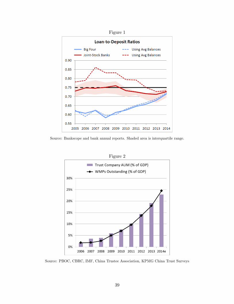
Figure 1

Source: Bankscope and bank annual reports. Shaded area is interquartile range.

Figure 2

Source: PBOC, CBRC, IMF, China Trustee Association, KPMG China Trust Surveys

39

Figure 3

Source: Wind Financial Terminal

Figure 4

Source: PBOC and Wind Financial Terminal

40

Figure 5

(a) Repo Lending by Big Banks (RMB Billions)

Note: Interest rate is the weighted average lending rate charged by big banks.

Excludes loans between big banks.

(b) Repo Lending by Policy Banks (RMB Billions)

Note: Interest rate is the weighted average lending rate charged by policy banks.

41

Figure 6

Note: The lending (borrowing) rate is the interest rate at which the bank

lends (borrows) on the interbank repo market.

Figure 7

Note: The interest rate refers to the rate on the interbank repo market.

42

Table 1

Calibration Results

(1) (2) (3) (4)

Model Data Model Data

α = 0.14 2007 α = 0.25 2014

Average Interbank Rate (πi`L + (1− π) ihL) 3.35% 3.1% 3.6% 3.6%

Small Bank WMPs (Wj) 0.03 NA 0.10 0.10

Big Bank WMPs (Wk) 0.01 NA 0.05 0.05

Big Bank Funding Share (Xk) 0.52 0.55 0.45 0.45

Big Bank Loan-to-Deposit Ratio (1− RkXk) 58% 62% 70% 70%

Credit-to-Savings Ratio (1−Rj −Rk) 72.1% 65% 75.3% 75%

Notes: We target the 2014 values of all variables in this table except for the credit-to-savings ratio.

The 2007 values of these variables as well as the 2007 and 2014 values of the credit-to-savings ratio

are generated by the calibrated model.

Table 2

Pairwise Correlations

iL ξj ξk

ξj 0.456 - -

(0.077)

ξk 0.329 0.736 -

(0.095) (0.052)

ξj − ξk 0.259 0.550 -0.152

(0.093) (0.088) (0.147)

Notes: Bootstrapped standard errors are in parentheses.

43

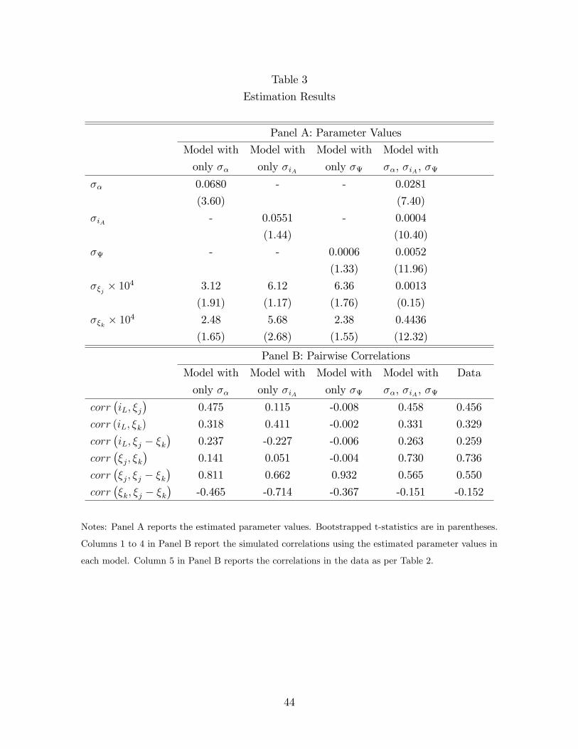
Table 3

Estimation Results

Panel A: Parameter Values

Model with Model with Model with Model with

only σα only σiA only σΨ σα, σiA , σΨ

σα 0.0680 - - 0.0281

(3.60) (7.40)

σiA - 0.0551 - 0.0004

(1.44) (10.40)

σΨ - - 0.0006 0.0052

(1.33) (11.96)

σξj × 104 3.12 6.12 6.36 0.0013

(1.91) (1.17) (1.76) (0.15)

σξk × 104 2.48 5.68 2.38 0.4436

(1.65) (2.68) (1.55) (12.32)

Panel B: Pairwise Correlations

Model with Model with Model with Model with Data

only σα only σiA only σΨ σα, σiA , σΨ

corr(iL, ξj

)0.475 0.115 -0.008 0.458 0.456

corr (iL, ξk) 0.318 0.411 -0.002 0.331 0.329

corr(iL, ξj − ξk

)0.237 -0.227 -0.006 0.263 0.259

corr(ξj, ξk

)0.141 0.051 -0.004 0.730 0.736

corr(ξj, ξj − ξk

)0.811 0.662 0.932 0.565 0.550

corr(ξk, ξj − ξk

)-0.465 -0.714 -0.367 -0.151 -0.152

Notes: Panel A reports the estimated parameter values. Bootstrapped t-statistics are in parentheses.

Columns 1 to 4 in Panel B report the simulated correlations using the estimated parameter values in

each model. Column 5 in Panel B reports the correlations in the data as per Table 2.

44

Appendix A —Proofs

Proof of Proposition 1

By contradiction. Suppose ρ > 0. If µj > 0, then Rj = 0 so equation (4) implies iL = θXψ.

Substituting into equation (9) then implies ξj > 0 if and only if φ < (1+iA)2−1X

− θ2X

ψX≡ φ1

(where we have used Xj = X in a symmetric equilibrium). If instead µj = 0, then equation

(7) implies iL = (1 + iA)2− 1. Substituting into equation (9) then implies ξj > 0 if and only

if φ < 1−θX

[(1 + iA)2 − 1

]≡ φ2. Defining φ ≡ min

φ1, φ2

completes the proof.

Proof of Proposition 2

With ρ = 0, the equilibrium is characterized by (4), (7), and:

ξj =αµj

2(1− θ

)µj[Rj − α

(X − ωξj

)]= 0 with complementary slackness

There is an implicit refinement here since we are writing ξj =αµj

2(1−θ)instead of ξj =

αµjτ j

2(1−θ).

Both produce ξj = 0 if αµj = 0 so the refinement only applies if αµj > 0. Return to

equations (8) and (9) with ρ = 0 and αµj > 0. If ξj > 0, then η1j > 0. This implies τ j = 1

which confirms ξj > 0. If ξj = 0, then η1j = η0

j . This implies τ j ∈ [0, 1]. However, any

τ j ∈ (0, 1] would return ξj > 0, violating ξj = 0. We thus eliminate ξj = 0 by refinement.

Instead, αµj > 0 is associated with ξj > 0 and thus τ j = 1. For this reason, we write

ξj =αµj

2(1−θ). We can now proceed with the rest of the proof. There are two cases:

1. If µj = 0, then ξj = 0 and 1 + iL = (1 + iA)2. Equation (4) then pins down Rj. To

ensure that Rj ≥ α(X − ωξj

)is satisfied, we need α ≤ θ− ψ[(1+iA)2−1]

X≡ α1. We have

now established ξj = 0 if α ≤ α1.

2. If µj > 0, then complementary slackness implies Rj = α(X − ωξj

). Combining with

the other equilibrium conditions, we find that µj > 0 delivers:

iL =α2ω

[(1 + iA)2 − 1

]− 2

(1− θ

) (α− θ

)X

α2ω + 2ψ(1− θ

) (22)

Verifying µj > 0 is equivalent to verifying 1 + iL < (1 + iA)2. This reduces to α > α1.

If α1 ≥ 0, then we have established ξj > 0 with τ j = 1 for any α > α1.

45

Defining α = max α1, 0 completes the proof.

Proof of Proposition 3

Consider α = 0. If µj = 0, then (7) implies iL = (1 + iA)2 − 1 which is the highest

feasible interbank rate. If instead µj > 0, then the liquidity rule binds. In particular,

Rj = α (Xj − τ jWj) which is just Rj = 0 when α = 0. We can then conclude iL = θXψfrom

(4). Note that µj > 0 is verified if and only if θXψ< (1 + iA)2 − 1.

Based on the results so far, we can see that the interbank rate at α = 0 is independent

of ρ. Let iL0 denote the interbank rate at α = 0 and let iL1 (ρ) denote the interbank rate at

some α > 0. From (4), we know iL1 (ρ) = θXψ− Rj1(ρ)

ψ, where Rj1 (ρ) is reserve holdings at

the α > 0 being considered. The rest of the proof proceeds by contradiction. In particular,

suppose iL1 (ρ) > iL0. Then α = 0 must be associated with µj > 0, otherwise iL0 would

be the highest feasible interbank rate and the supposition would be incorrect. We can thus

write iL0 = θXψand iL1 (ρ) = iL0− Rj1(ρ)

ψ. The only way to get iL1 (ρ) > iL0 is then Rj1 (ρ) < 0

which is impossible.

Proof of Proposition 4

Start with general α. The derivatives of the big bank’s objective function are:

∂Υk

∂ξk∝ −

2ω(1− θ

)1− π ξk −

[(1 + iA)2 − 1

1− π − ihL

]∂Rk

∂ξk+

[(1 + iA)2 − 1− φXk

1− π − θhihL

]∂Xk

∂ξk

∂Υk

∂ihL∝ Rk − θhXk −

[(1 + iA)2 − 1

1− π − ihL

]∂Rk

∂ihL+

[(1 + iA)2 − 1− φXk

1− π − θhihL

]∂Xk

∂ihL

It will be convenient to reduce these derivatives to a core set of variables (ξj, ξk, and ihL). If

µj > 0, then the complementary slackness in equation (13) implies:

Rj = α(Xj − ωξj

)(23)

With δ1 + δ2 = 0 and ξj = ξj, equations (10) and (11) are:

Xj = 1− δ0 + δ1

(ξj − ξk

)(24)

Xk = δ0 + δ1

(ξk − ξj

)(25)

Substitute (23) to (25) into equation (12) to write:

46

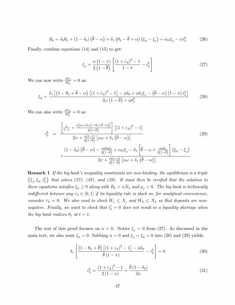
Rk = δ0θh + (1− δ0)(θ − α

)+ δ1

(θh − θ + α

) (ξk − ξj

)+ αωξj − ψihL (26)

Finally, combine equations (14) and (15) to get:

ξj =α (1− π)

2(1− θ

) [(1 + iA)2 − 1

1− π − ihL

](27)

We can now write ∂Υk∂ξk

= 0 as:

ξk =δ1

[(1− θh + θ − α

) [(1 + iA)2 − 1

]− φδ0 + φδ1ξj −

(θ − α

)(1− π) ihL

]2ω(1− θ

)+ φδ2

1

(28)

We can also write ∂Υk∂ihL

= 0 as:

ihL =

[ψ

1−π +α[αω+δ1(1−θh+θ−α)]

2(1−θ)

] [(1 + iA)2 − 1

]2ψ + α(1−π)

2(1−θ)

[αω + δ1

(θ − α

)] (29)

+

(1− δ0)(θ − α

)− αφδ0δ1

2(1−θ)+ αωξj − δ1

[θ − α + αφδ1

2(1−θ)

] (ξk − ξj

)2ψ + α(1−π)

2(1−θ)

[αω + δ1

(θ − α

)]Remark 1 If the big bank’s inequality constraints are non-binding, the equilibrium is a tripleξj, ξk, i

hL

that solves (27), (28), and (29). It must then be verified that the solution to

these equations satisfies ξk ≥ 0 along with Rk > αXk and µj > 0. The big bank is technically

indifferent between any τ k ∈ [0, 1] if its liquidity rule is slack so, for analytical convenience,

consider τ k = 0. We also need to check Wj ≤ Xj and Wk ≤ Xk so that deposits are non-

negative. Finally, we want to check that i`L = 0 does not result in a liquidity shortage when

the big bank realizes θ` at t = 1.

The rest of this proof focuses on α = 0. Notice ξj = 0 from (27). As discussed in the

main text, we also want ξk = 0. Subbing α = 0 and ξj = ξk = 0 into (28) and (29) yields:

δ1

[(1− θh + θ

) [(1 + iA)2 − 1

]− φδ0

θ (1− π)− ihL

]= 0 (30)

ihL =(1 + iA)2 − 1

2 (1− π)+θ (1− δ0)

2ψ(31)

47

To verify ξk = 0, we must verify that (30) holds when ihL is given by (31). This requires

either δ1 = 0 or:

φ =1

δ0

[1− θh +

θ

2

] [(1 + iA)2 − 1

]− θ

2(1− π) (1− δ0)

2ψδ0

≡ φ∗ (32)

In other words, we can use either δ1 = 0 or the combination of δ1 > 0 and φ = φ∗ to get ξkexactly zero at α = 0. Note that Wj ≤ Xj and Wk ≤ Xk are trivially true with ξj = ξk = 0.

We now need to check Rk > αXk and µj > 0. Using (14) and (31), rewrite µj > 0 as:

(1 + iA)2 − 1

1− π >θ (1− δ0)

ψ(33)

Note that condition (33) is also suffi cient for φ∗ > 0. With µj > 0 verified, we can substitute

α = 0 into equation (23) to get Rj = 0. The next step is to check Rk > αXk which is simply

Rk > 0 at α = 0. Recall that Rk is given by equation (26). Use α = 0 and ξj = ξk = 0 along

with ihL as per (31) to rewrite equation (26) as:

Rk = θhδ0 +θ (1− δ0)

2− ψ (1 + iA)2 − 1

2 (1− π)(34)

The condition for Rk > 0 is therefore:

(1 + iA)2 − 1

1− π <θ (1− δ0)

ψ+

2δ0θhψ

(35)

The last step is to check that there is suffi cient liquidity at t = 1 when the big bank’s

liquidity shock is low. The demand for liquidity in this case will be θXj + θ`Xk. The supply

of liquidity will be Rj + Rk since we have fixed i`L = 0. We already know ξj = ξk = 0 at

α = 0. Therefore, Xj = 1 − δ0 and Xk = δ0. We also know Rj = 0 and Rk as per (34).

Therefore, Rj +Rk ≥ θXj + θ`Xk can be rewritten as:

(1 + iA)2 − 1

1− π ≤ 2δ0 (θh − θ`)ψ

− θ (1− δ0)

ψ(36)

Condition (36) is stricter than (35) so we can drop (35). We now just need to make sure

that conditions (33) and (36) are not mutually exclusive. Using θ ≡ πθ` + (1− π) θh, this

requires:

θ` <

[1− 1− δ0

δ0 + π (1− δ0)

]θh (37)

48

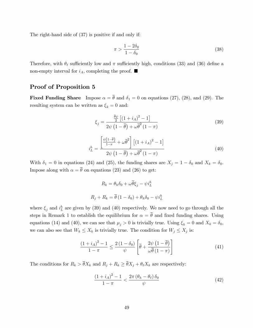
The right-hand side of (37) is positive if and only if:

π >1− 2δ0

1− δ0

(38)

Therefore, with θ` suffi ciently low and π suffi ciently high, conditions (33) and (36) define a

non-empty interval for iA, completing the proof.

Proof of Proposition 5

Fixed Funding Share Impose α = θ and δ1 = 0 on equations (27), (28), and (29). The

resulting system can be written as ξk = 0 and:

ξj =θψ2

[(1 + iA)2 − 1

]2ψ(1− θ

)+ ωθ

2(1− π)

(39)

ihL =

[ψ(1−θ)

1−π + ωθ2] [

(1 + iA)2 − 1]

2ψ(1− θ

)+ ωθ

2(1− π)

(40)

With δ1 = 0 in equations (24) and (25), the funding shares are Xj = 1 − δ0 and Xk = δ0.

Impose along with α = θ on equations (23) and (26) to get:

Rk = θhδ0 + ωθξj − ψihL

Rj +Rk = θ (1− δ0) + θhδ0 − ψihL

where ξj and ihL are given by (39) and (40) respectively. We now need to go through all the

steps in Remark 1 to establish the equilibrium for α = θ and fixed funding shares. Using

equations (14) and (40), we can see that µj > 0 is trivially true. Using ξk = 0 and Xk = δ0,

we can also see that Wk ≤ Xk is trivially true. The condition for Wj ≤ Xj is:

(1 + iA)2 − 1

1− π ≤ 2 (1− δ0)

ψ

[θ +

2ψ(1− θ

)ωθ (1− π)

](41)

The conditions for Rk > θXk and Rj +Rk ≥ θXj + θ`Xk are respectively:

(1 + iA)2 − 1

1− π <2π (θh − θ`) δ0

ψ(42)

49

(1 + iA)2 − 1

1− π ≤2ψ(1− θ

)+ ωθ

2(1− π)

ψ(1− θ

)+ ωθ

2(1− π)

(θh − θ`) δ0

ψ(43)

Now, for the interbank rate to increase when moving from α = 0 to α = θ, we need (40) to

exceed (31). Equivalently, we need:

(1 + iA)2 − 1

1− π >θ (1− δ0)

ψ

[1 +

2ψ(1− θ

)ωθ

2(1− π)

](44)

We must now collect all the conditions involved in the α = 0 and α = θ equilibria and

make sure they are mutually consistent. There are two lowerbounds on iA, namely (33) and

(44). Condition (44) is clearly stricter so it is the relevant lowerbound. There are also four

upperbounds on iA, namely (36), (41), (42), and (43). For the lowerbound in (44) to not

violate any of these upperbounds, we need:

ψ(1− θ

)ω (1− π)

< θ2

min

π (θh − θ`) δ0

θ (1− δ0)− 1

2,(θh − θ`) δ0

θ (1− δ0)− 1

This inequality is only possible if the right-hand side is positive. Therefore, we need:

θ` <

[1− 1− δ0

min δ0 + π (1− δ0) , π (1 + δ0)

]θh (45)

Once again, the right-hand side must be positive so we need:

π > max

1− 2δ0

1− δ0

,1− δ0

1 + δ0

(46)

Notice that (45) and (46) are just refinements of (37) and (38). We can now conclude that the

model with fixed funding shares generates the desired results under the following conditions:

π suffi ciently high, θ` andψωsuffi ciently low, and iA within an intermediate range.

Endogenous Funding Share Return to equations (27), (28), and (29). Impose α = θ

and δ1 = ω with φ = φ∗ as per (32). Combine to get:

ihL =(1 + iA)2 − 1

1− π −

[2ψ

1−π + ωθ2

2(1−θ)+φ∗ω

](1+iA)2−1

2(1−π)− ωθ

3(1−δ0)

2ψ[2(1−θ)+φ∗ω]

2ψ1−π + ωθ

2

2(1−θ)

[2 + φ∗ω

2(1−θ)+φ∗ω

] (47)

50

ξk =

θ(1−π)2

[θ(1−δ0)

ψ+(φ∗ω1−θ − 1

)(1+iA)2−1

1−π − φ∗ω1−θ i

hL

]2(1− θ

)+ φ∗ω

(48)

We now need to go through the steps in Remark 1 to establish the equilibrium for α = θ

and endogenous funding shares. The expressions here are more complicated so we proceed

by finding one value of iA that satisfies all the steps in Remark 1. A continuity argument

will then allow us to conclude that all the steps are satisfied for a non-empty range of iA.

Consider iA such that:(1 + iA)2 − 1

1− π =θ

ψ(49)

Substituting into (32) then pins down φ∗ as:

φ∗ =θ (1− π)

ψ

[1− θhδ0

+θ

2

](50)

From the proof of Proposition 4, we already have (33) and (36) as restrictions on iA. We

also have (37) as an upperbound on θ` and (38) as a lowerbound on π. It is easy to see that

iA as defined in (49) satisfies (33). For (49) to also satisfy (36), we need:

θ` <

[1− 2− δ0

2δ0 + π (2− δ0)

]θh (51)

π >2− 3δ0

2− δ0

(52)

Conditions (51) and (52) are stricter than (37) and (38). We can thus drop (37) and (38).

The first step is to verify µj > 0. Use (14) and (47) to write µj > 0 as:

(1 + iA)2 − 1

1− π

[1 +

2ψ[2(1− θ

)+ φ∗ω

]ωθ

2(1− π)

]>θ (1− δ0)

ψ

This is true by condition (33).

The second step is to verify ξk > 0. Substituting (47) into (48), we see that we need:

(1 + iA)2 − 1

1− π

1− φ∗

2(1−θ)ω

+ θ2(1−π)ψ

< θ (1− δ0)

ψ(53)

51

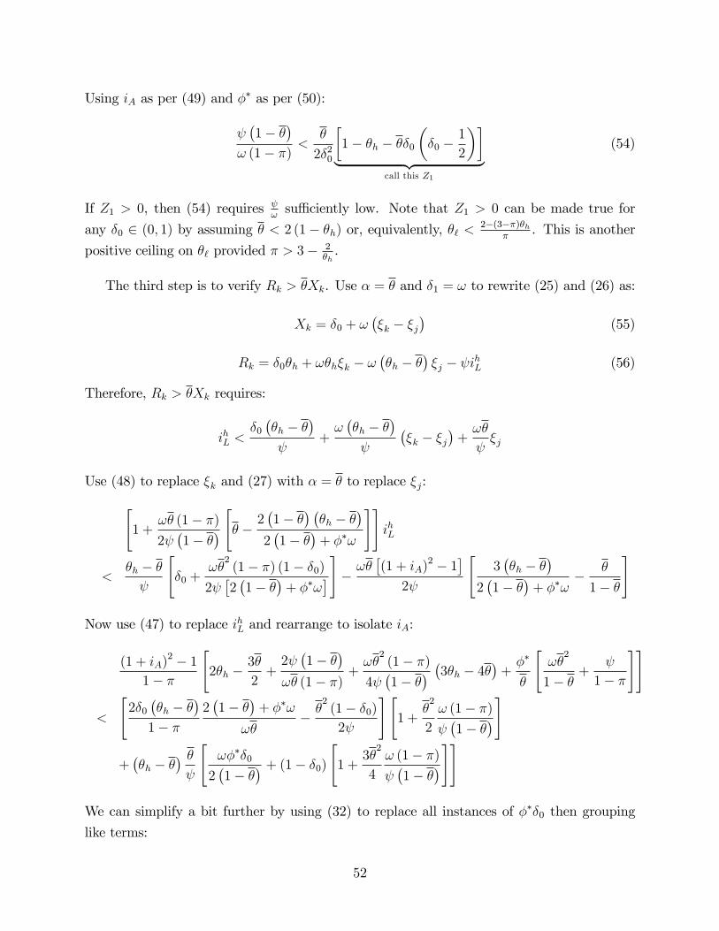
Using iA as per (49) and φ∗ as per (50):

ψ(1− θ

)ω (1− π)

<θ

2δ20

[1− θh − θδ0

(δ0 −

1

2

)]︸ ︷︷ ︸

call this Z1

(54)

If Z1 > 0, then (54) requires ψωsuffi ciently low. Note that Z1 > 0 can be made true for

any δ0 ∈ (0, 1) by assuming θ < 2 (1− θh) or, equivalently, θ` < 2−(3−π)θhπ

. This is another

positive ceiling on θ` provided π > 3− 2θh.

The third step is to verify Rk > θXk. Use α = θ and δ1 = ω to rewrite (25) and (26) as:

Xk = δ0 + ω(ξk − ξj

)(55)

Rk = δ0θh + ωθhξk − ω(θh − θ

)ξj − ψihL (56)

Therefore, Rk > θXk requires:

ihL <δ0

(θh − θ

)ψ

+ω(θh − θ

)ψ

(ξk − ξj

)+ωθ

ψξj

Use (48) to replace ξk and (27) with α = θ to replace ξj:[1 +

ωθ (1− π)

2ψ(1− θ

) [θ − 2(1− θ

) (θh − θ

)2(1− θ

)+ φ∗ω

]]ihL

<θh − θψ

[δ0 +

ωθ2

(1− π) (1− δ0)

2ψ[2(1− θ

)+ φ∗ω

]]− ωθ[(1 + iA)2 − 1

]2ψ

[3(θh − θ

)2(1− θ

)+ φ∗ω

− θ

1− θ

]

Now use (47) to replace ihL and rearrange to isolate iA:

(1 + iA)2 − 1

1− π

[2θh −

3θ

2+

2ψ(1− θ

)ωθ (1− π)

+ωθ

2(1− π)

4ψ(1− θ

) (3θh − 4θ)

+φ∗

θ

[ωθ

2

1− θ+

ψ

1− π

]]

<

[2δ0

(θh − θ

)1− π

2(1− θ

)+ φ∗ω

ωθ− θ

2(1− δ0)

2ψ

][1 +

θ2

2

ω (1− π)

ψ(1− θ

)]

+(θh − θ

) θψ

[ωφ∗δ0

2(1− θ

) + (1− δ0)

[1 +

3θ2

4

ω (1− π)

ψ(1− θ

)]]

We can simplify a bit further by using (32) to replace all instances of φ∗δ0 then grouping

like terms:

52

(1 + iA)2 − 1

1− π

θh − θ2

+2ψ(1−θ)ωθ(1−π)

− ωθ3(1−π)

4ψ(1−θ)+ φ∗

θ

[ωθ

2

1−θ + ψ1−π

]−(θh − θ

)(1− θh)

[2θ

+ 3θ2ω(1−π)

ψ(1−θ)

]

<

[4δ0

(1− θ

) (θh − θ

)ωθ (1− π)

− θ2

(1− δ0)

2ψ

][1 +

θ2

2

ω (1− π)

ψ(1− θ

)]

Substitute iA as per (49) and φ∗ as per (50) then rearrange:

ψ(1− θ

)ω (1− π)

[θh −

θ (1 + δ0)

2+

[θ +

1− θhδ0

+2

θ

ψ(1− θ

)ω (1− π)

][1−

2δ0

(θh − θ

)θ

]](57)

<θ

δ0

[θ

2δ2

0

4+δ0

2

[3(θh − θ

)(1− θh)− θ

2]− θ (1− θh)

]︸ ︷︷ ︸

call this Z2

Condition (57) will be true for ψωsuffi ciently low if Z2 > 0. Use θ ≡ πθ` + (1− π) θh to

rewrite Z2 > 0 as:

π2 (θh − θ`)2 − 2

[θh +

(2 + 3δ0) (1− θh)δ0 (2− δ0)

]π (θh − θ`) + θh

[θh +

4 (1− θh)δ0 (2− δ0)

]< 0

Based on the roots of this quadratic, we can conclude that Z2 > 0 requires:

π (θh − θ`) > θh +(2 + 3δ0) (1− θh)

δ0 (2− δ0)−

√√√√1− θh2− δ0

(6θh +

(2 + 3δ0)2 (1− θh)δ2

0 (2− δ0)

)(58)

Condition (58) is satisfied by θ` = 0 and π = 1. The left-hand side is decreasing in θ` and

increasing in π so it follows that Z2 > 0 requires θ` suffi ciently low and π suffi ciently high.

The fourth step is to verify Wj ≤ Xj. Use Wj = ωξj and (24) with δ1 = ω to rewrite

Wj ≤ Xj as:

ξk ≤1− δ0

ω

Now use (48) with ihL as per (47) to replace ξk. Substitute iA as per (49) and φ∗ as per (50).

Rearrange to isolate all terms withψ(1−θ)ω(1−π)

on one side. The condition for Wj ≤ Xj becomes:

53

ψ(1− θ

)ω (1− π)

[θ

2

2+ (1− δ0)

[θ

2+θ (1− θh)

δ0

+ 2ψ(1− θ

)ω (1− π)

]](59)

≥ θ3

4

[(1− θh)

(3− 2

δ0

)− θ

(1− δ0

2

)]︸ ︷︷ ︸

call this Z3

A suffi cient condition for Z3 < 0, and hence Wj ≤ Xj, is δ0 ≤ 23.

The fifth step is to verify Wk ≤ Xk. Use Wk = ωξk and (55) to rewrite Wk ≤ Xk as:

ξj ≤δ0

ω

Now use (27) with α = θ and ihL as per (47) to replace ξj. Substitute iA as per (49) and

φ∗ as per (50). Rearrange to isolate all terms withψ(1−θ)ω(1−π)

on one side. The condition for

Wk ≤ Xk becomes:

ψ(1− θ

)ω (1− π)

[1− 3δ0 −

2δ0

θ

[1− θhδ0

+2

θ

ψ(1− θ

)ω (1− π)

]](60)

≤ θ

2

[(1− θh)

(3− 1

δ0

)− θ

(1

2− δ0

)]︸ ︷︷ ︸

call this Z4

Condition (60) will be true for ψωsuffi ciently low if Z4 > 0. Use the definition of θ to rewrite

Z4 > 0 as:

π (θh − θ`) δ0 (1− 2δ0) > θhδ0 (1− 2δ0)− 2 (1− θh) (3δ0 − 1) (61)

If δ0 ≥ 12, then (61) is always true. If δ0 <

12, then (61) reduces to:

θ` <1

π

[2 (1− θh) (3δ0 − 1)

δ0 (1− 2δ0)− θh (1− π)

]This is a positive ceiling on θ` provided π > 1 − 2(1−θh)(3δ0−1)

θhδ0(1−2δ0)with δ0 >

13. Therefore, (61)

is guaranteed by θ` suffi ciently low, π suffi ciently high, and δ0 >13.

The sixth step is to verify feasibility of i`L = 0. This requires Rj +Rk ≥ θXj + θ`Xk. Use

(23) with α = θ to replace Rj. The desired inequality becomes:

54

Rk ≥ θ`Xk + ωθξj

Substituting Xk and Rk as per equations (55) and (56):

ihL ≤θh − θ`ψ

[δ0 + ω

(ξk − ξj

)]Use (48) to replace ξk. Also use (27) with α = θ to replace ξj. Rearrange to isolate i

hL then

use (47) to replace ihL. Substitute iA as per (49) and φ∗ as per (50). Rearrange to isolate all

terms withψ(1−θ)ω(1−π)

on one side. The feasibility condition for i`L = 0 becomes:

ψ(1− θ

)ω (1− π)

θ(5−δ0)4− (θh − θ`)

[1−θhθ

+ 2δ0−12

]+1−θh

2δ0+[1− 2(θh−θ`)δ0

θ

]1θ

ψ(1−θ)ω(1−π)

≤ 3θ

4

[(1− θh)

[θh − θ` −

θ

δ0

]− θ

2

2

]︸ ︷︷ ︸

call this Z5

(62)

Condition (62) will be true for ψωsuffi ciently low if Z5 > 0. Use the definition of θ to rewrite

Z5 > 0 as:

π2 (θh − θ`)2 − 2

[πθh +

(π + δ0) (1− θh)δ0

](θh − θ`) + θh

[θh +

2 (1− θh)δ0

]< 0

Based on the roots of this quadratic, we can conclude that Z5 > 0 requires:

θ` <1

π2

√2πθh (1− θh) +(π + δ0)2 (1− θh)2

δ20

− (π + δ0) (1− θh)δ0

− θhπ (1− π)

This is a positive upperbound on θ` provided

θh(1−π)2

2(1−θh)+ 1−π

δ0< 1. Therefore, Z5 > 0 requires

θ` suffi ciently low and π suffi ciently high.

It now remains to check that the interbank rate increases when moving from α = 0 to

α = θ. This requires (47) to exceed (31) or, equivalently:

(1 + iA)2 − 1

1− π > (1− δ0)

[θ

ψ+

4(1− θ

)ωθ (1− π)

2(1− θ

)+ φ∗ω

2(1− θ

)+ 3φ∗ω

]

Using iA as per (49) and φ∗ as per (50):

55

ψ(1− θ

)ω (1− π)

[1− θhδ0

+θ (1− 2δ0)

2 (1− δ0)+

2

θ

ψ(1− θ

)ω (1− π)

]<

3θ2

4 (1− δ0)

[1− θh +

θδ0

2

](63)

The right-hand side is positive so (63) will be true for ψωsuffi ciently low.

Putting everything together, we have shown that the model with endogenous funding

shares generates the desired results under the following conditions: π suffi ciently high, θ`and ψ

ωsuffi ciently low, δ0 ∈

(13, 2

3

), and iA as per (49). The results then extend to a non-empty

range of iA by continuity.

Comparison We now compare the interbank rate increases in the fixed share and endoge-

nous share models. Notice from the proof of Proposition 4 that the interbank rate at α = 0

is the same in both models. Therefore, we just need to show that the interbank rate in the

endogenous share model exceeds the interbank rate in the fixed share model at α = θ. In

other words, we need to show that (47) exceeds (40) for a given set of parameters. This

reduces to:

(1 + iA)2 − 1

1− π

1− φ∗

2(1−θ)ω

+ θ2(1−π)ψ

< θ (1− δ0)

ψ

which is exactly (53), where (53) was the condition for ξk > 0 at α = θ in the endogenous

share model. To complete the proof, we must now show that there are indeed parameters that

satisfy the conditions in both models. For α = 0, we imposed conditions (33) and (36) along

with π suffi ciently high and θ` suffi ciently low. These conditions applied to both models. For

α = θ in the fixed share model, we also imposed conditions (41), (42), (43), and (44) along

with ψωsuffi ciently low. For α = θ in the endogenous share model, we added δ0 ∈

(13, 2

3

)and

iA in the neighborhood of (49). In (51) and (52), we showed that π suffi ciently high and θ`suffi ciently low make (49) satisfy condition (36). We have also shown that condition (44) is

stricter than condition (33). Therefore, we just need to show that (49) satisfies conditions

(41), (42), (43), and (44). Substituting iA as per (49) into these conditions produces the

following inequalities which we must check:

ψ(1− θ

)ω (1− π)

>θ

2(2δ0 − 1)

4 (1− δ0)(64)

θ` <

[1− 1

π (1 + 2δ0)

]θh (65)

56

ψ(1− θ

)ω (1− π)

[1− 2 (θh − θ`) δ0

θ

]< θ

2[

(θh − θ`) δ0

θ− 1

](66)

ψ(1− θ

)ω (1− π)

<θ

2δ0

2 (1− δ0)(67)

A suffi cient condition for (64) is δ0 ≤ 12which is still consistent with δ0 ∈

(13, 2

3

). Condition

(65) is just another positive upperbound on θ` provided π > 11+2δ0

. In other words, (65)

is satisfied by θ` suffi ciently low and π suffi ciently high. Condition (66) will be true forψω

suffi ciently low if (θh − θ`) δ0 > θ or, equivalently, θ` <[1− 1

δ0+π

]θh with π > 1− δ0 which

again means θ` suffi ciently low and π suffi ciently high. Finally, condition (67) is clearly

satisfied by ψωsuffi ciently low.

Proof of Proposition 6

Evaluate (27) at α = θ then subtract (48) to get:

ξj − ξksign=

[(1 + iA)2 − 1

1− π − θ (1− δ0)

ψ

]+ 2

[(1 + iA)2 − 1

1− π − ihL

]

The expression in the first set of square brackets is positive by condition (33). The expression

in the second set of square brackets is proportional to µj. The proof of Proposition 5

established µj > 0. Therefore, ξj > ξk at α = θ.

Now consider total credit:

TC ≡ 1−Rj −Rk

Use market clearing as per (12) to replace Rj +Rk:

TC = 1− θXj − θhXk + ψihL

Use (24) and (25) to replace Xj and Xk:

TC = 1− θ −(θh − θ

)δ0 + δ1

(θh − θ

) (ξj − ξk

)+ ψihL

Proposition 5 showed ihL∣∣α=θ

> ihL∣∣α=0. We also know ξj = ξk = 0 at α = 0 and ξj > ξk at

α = θ. Therefore, we can conclude TC|α=θ > TC|α=0.

Finally, we want to show that the loan-to-deposit ratios of big and small banks converge.

The equilibrium has τ j = 1, meaning that small banks move all DLPs (and the associated

57

investments) off-balance-sheet. The loan-to-deposit ratio of the representative small bank is

then λj ≡ 1 − RjXj−Wj

. The equilibrium also has τ k = 0, meaning that the big bank records

everything on-balance-sheet. Its loan-to-deposit ratio is then λk ≡ 1 − RkXk. Proposition

4 established Rk > 0 = Rj at α = 0 so it follows that λk|α=0 < 1 = λj|α=0. To show

convergence, we just need to show λk|α=θ > λk|α=0 since λj|α=θ < λj|α=0 follows immediately

from equation (23). Use Xj +Xk = 1 along with the definition of λk to rewrite (12) as:

ψihL = θ +[θh − θ − (1− λk)

]Xk −Rj

We know ihL∣∣α=θ

> ihL∣∣α=0

so it must be the case that:

[θh − θ − (1− λk|α=θ)

]Xk|α=θ − Rj|α=θ >

[θh − θ − (1− λk|α=0)

]Xk|α=0

Proposition 4 also established ξj = ξk = 0 at α = 0. Substituting into equation (25) then

implies Xk = δ0 at α = 0 so:

λk|α=θ

Xk|α=θ

δ0

− λk|α=0 >Rj|α=θ

δ0

− [1− π (θh − θ`)][1− Xk|α=θ

δ0

]︸ ︷︷ ︸

call this Z6

We have shown ξj > ξk at α = θ so equation (25) also implies Xk|α=θδ0

≤ 1 for any δ1 ≥ 0.

Therefore, Z6 ≥ 0 will be suffi cient for λk|α=θ > λk|α=0. If δ1 = 0, then Z6 ∝ Rj|α=θ ≥ 0. If

δ1 = ω, then we can rewrite Z6 ≥ 0 as:

1− δ0 − ωξk ≥1− π (θh − θ`)

θω(ξj − ξk

)(68)

where ξj is given by (27) with α = θ and ξk is given by (48). Use these expressions to

substitute out ξj and ξk then use equation (47) to substitute out ihL. Evaluate iA at (49) and

φ∗ at (50) to rewrite (68) as:

4ψ(1− θ

)(1− δ0)

ωθ (1− π)+ θ (2− 3δ0) + (1− θh)

(2

δ0

− 3− δ0

)︸ ︷︷ ︸

call this ∆(δ0)

≥ −θ2

4

ω (1− π)

ψ(1− θ

)[2θ (1− 2δ0) + (1− θh)(

4

δ0

− 6− 3δ0

)]︸ ︷︷ ︸

call this ∆(δ0)

58

A suffi cient condition for this is min

∆ (δ0) , ∆ (δ0)≥ 0. Notice ∆′ (·) < 0 and ∆′ (·) < 0.

Also notice min

∆(

12

), ∆(

12

)> 0 and min

∆(

23

), ∆(

23

)< 0. Therefore, there is a

threshold δ0 ∈(

12, 2

3

)such that δ0 ≤ δ0 guarantees Z6 ≥ 0.

Appendix B —Deposit and DLP Demands

Here we sketch a simple household maximization problem which generates the demands in

equations (1) and (2). There is a continuum of ex ante identical households indexed by

i ∈ [0, 1]. Each household is endowed with X units of funding. Let Dij and Wij denote the

deposits and DLPs purchased by household i from bank j, where:∑j

(Dij +Wij) ≤ X (69)

Assume that buying Wij entails a transaction cost of 12ω0W 2ij, where ω0 > 0. As per the

main text, the interest rate on the DLP is zero if withdrawn early and ξj otherwise. The

interest rate on deposits is always zero and the average probability of early withdrawal is

θ. The household requires subsistence consumption of X in each state, above which it is

risk neutral. If the household were to bypass the banking system and invest in long-term

projects directly, it would fall below subsistence in the state where it needs to liquidate early

since long-term projects cannot be liquidated early. Therefore, the household does not invest

directly. Instead, it chooses Dij and Wij for each j to maximize:

∑j

(Dij +

[1 +

(1− θ

)ξj]Wij −

W 2ij

2ω0

)

subject to (69) holding with equality.26 The first order condition with respect to Wij is:

Wij =(1− θ

)ω0ξj (70)

Substituting (70) into (69) when the latter holds with equality gives the household’s total

deposit demand, Di ≡∑

j Dij. The household is indifferent about the allocation of Di across

26Here is how to recover the two-point distribution of idiosyncratic bank shocks in Section 2 from thehousehold withdrawals. Each household has probability θ` of being hit by an idiosyncratic consumptionshock at t = 1 and having to withdraw all of its funding early. This results in each bank losing fraction θ`of its deposits and DLPs at t = 1. Then θh − θ` of the remaining 1− θ` households observe a sunspot andwithdraw all of their funding from 1− π banks at t = 1. The θh − θ` households and 1− π banks involvedin the sunspot are chosen at random. Note θ ≡ πθ` + (1− π) θh.

59

banks so we assume that it simply allocates Di uniformly. For J banks, this yields:

Dij =X

J−(1− θ

)ω0

Jξj −

(J − 1)(1− θ

)ω0

J

1

J − 1

∑x 6=j

ξx (71)

With a unit mass of ex ante identical households,Wj = Wij andDj = Dij. As J approaches a

unit mass of equally-weighted banks, (70) and (71) belong to the family of functions specified

by (1) and (2).

Appendix C —Benchmark with Aggregate Shock

Consider the benchmark model (only price-taking banks) in Section 2 but with an aggregate

interbank shock. In particular, the interbank rate is i`L with probability π and ihL with

probability 1−π. The expected interbank rate is ieL ≡ πi`L + (1− π) ihL. We will specify how

i`L and ihL are determined shortly. In the meantime, banks take both as given.

The objective function of the representative bank simplifies to:

Υj = (1 + iA)2 (Xj −Rj) + (1 + ieL)Rj −[Xj + ieLθXj +

(1− θ

)ξjWj

]− φ

2X2j

This is identical to the benchmark model except with the expected interbank rate ieL instead

of the deterministic iL. Therefore, the first order conditions are still given by equations (7)

to (9) but with ieL in place of iL.

The goal is to show that ieL is always highest at α = 0. The proof follows Proposition 3

but, to proceed, we must replace the deterministic market clearing condition (equation (4))

with conditions for each realization of the aggregate shock. We model the shock as a shock

to the aggregate demand for liquidity at t = 1. In particular, aggregate liquidity demand is

θX − ε with probability π and θX with probability 1− π, where ε > 0. The interbank rates

are then i`L and ihL respectively. To avoid liquidity shortages, we need these rates to satisfy:

Rj + ψi`L ≥ θX − ε (72)

Rj + ψihL ≥ θX (73)

The equilibrium ihL solves (73) with equality. If ihL ≤ ε

ψ, then we can set i`L = 0. Otherwise,

the equilibrium i`L solves (72) with equality.

60

Let ieL0 denote the expected interbank rate at α = 0 and let ieL1 (ρ) denote the expected

interbank rate at some α > 0. Using (72) and (73), we can write:

ieL1 (ρ) =θX

ψ− Rj1 (ρ)

ψ− π

ψmin

θX −Rj1 (ρ) , ε

(74)

where Rj1 (ρ) is reserve holdings at the α > 0 being considered. The proof of ieL1 (ρ) ≤ ieL0

proceeds by contradiction. In particular, suppose ieL1 (ρ) > ieL0. Then (7) implies µj > 0 at

α = 0. Complementary slackness then implies Rj = 0 at α = 0 so we can write:

ieL =θX

ψ− π

ψmin

θX, ε

(75)

Subtract (75) from (74) to get:

ieL1 (ρ) = ieL0 −Rj1 (ρ)

ψ+π

ψ

[min

θX, ε

−min

θX −Rj1 (ρ) , ε

]There are three cases. If ε ≤ θX −Rj1 (ρ), then:

ieL1 (ρ) = ieL0 −Rj1 (ρ)

ψ

If θX −Rj1 (ρ) < ε < θX, then:

ieL1 (ρ) = ieL0 −1− πψ

Rj1 (ρ)− π

ψ

(θX − ε

)If θX ≤ ε, then:

ieL1 (ρ) = ieL0 −1− πψ

Rj1 (ρ)

In each case, ieL1 (ρ) > ieL0 would require Rj1 (ρ) < 0 which is impossible.

Appendix D —Supplementary Material on China

Reforms We start with the market-oriented reforms initiated in the 1990s. The first effect

of these reforms was to make the Big Four much more profit-driven. All went through a major

restructuring in the mid-2000s and are now publicly listed. The government and the Big

Four still have ties which limit how intensely the Big Four compete against each other (e.g.,

the government holds controlling interest and appoints bank executives) but the government

61

is no longer involved in decisions at the operational level. The effect of the reforms has been

striking. The average non-performing loan ratio of the Big Four, which had ballooned to

30% by the early 2000s, has remained around 2% in recent years. Combined profits also

grew 19% annually from 2007 to 2014 to reach an unprecedented USD 184 billion in 2014.

Individually, the banks in China’s Big Four now constitute the first, second, fourth, and

seventh largest banks in the world as measured by total assets.27

The second effect of the reforms was entry of small and medium-sized commercial banks.28

These banks are still individually small when compared to the Big Four. For example, average

deposits for the JSCBs were only 17% of average deposits for the Big Four in 2013. As a

group though, small and medium-sized banks have chipped away at the Big Four’s deposit

share. In 1995, the Big Four held 80% of deposits in China. By 2005, they held 60%. The Big

Four now account for roughly 50% of traditional deposits, meaning that their deposit share

declined even after the major restructuring of the mid-2000s. To put this into perspective,

big state-owned firms in the industrial sector did not experience a similar post-restructuring

decline in market share. As we will see in the calibration, our model can account for the

post-restructuring decline of the Big Four.

Regulations Turning now to China’s regulatory environment, let us elaborate on the

evolution of reserve requirements, deposit rate regulation, and capital requirements.

Reserve Requirements Offi cial reserve requirements were 7.5% in 2005. There was a

modest increase to 9.5% by early 2007 as part of a policy to sterilize the accumulation of

foreign reserves without issuing central bank bills (Song, Storesletten, and Zilibotti (2014)).

Reserve requirements were then rapidly increased in a manner complementary to the in-

creasing frequency of CBRC’s loan-to-deposit checks, hitting 15.5% by February 2010 before

being raised another twelve times to reach 21.5% by December 2011.29 China lifted the

offi cial loan-to-deposit component of its liquidity rules in late 2015 but reserve requirements

remain high and loan-to-deposit restrictions can still technically be imposed via loan quotas

so there has been little dismantling of off-balance-sheet infrastructures.

27http://www.relbanks.com/worlds-top-banks/assets28These market-oriented reforms also paved the way for China’s rising private sector. For more, see Allen,

Qian, and Qian (2005), Hsieh and Klenow (2009), Song, Storesletten, and Zilibotti (2011), Brandt, VanBiesebroeck, and Zhang (2012), Lardy (2014), Hsieh and Song (2015), and the references therein.29In practice, a reserve requirement is a narrower type of liquidity regulation than a loan-to-deposit cap

because, unlike the latter, it specifies the form in which liquidity must be held. We abstracted from thisdifference in the model (i.e., liquid assets were reserves) but it is useful to point out the distinction here toavoid confusion about what the true liquidity requirement is. With a 75% loan-to-deposit cap, the liquidityrequirement is always 25%: a reserve requirement of x < 25% just means that the bank has discretion overhow to divide 25%− x between reserves and other liquid (i.e., non-loan) assets.

62

Deposit Rate Regulation China has a long history of regulating interest rates on tradi-

tional deposits. Prior to 2004, the central bank simply set these rates. Downward flexibility

was introduced in 2004 with no response: all banks stayed at the maximum allowable rate.

Some upward flexibility was then introduced in 2012 and almost all banks for which we have

systematic data responded by moving up to the new maximum. The highest deposit rate

allowed by the central bank thus continued to serve as the effective deposit rate in China.

In October 2015, China announced the removal of deposit rate ceilings. The response of

deposit rates has been modest. This is consistent with the most interest-sensitive savings

having already migrated to high-yielding WMPs.

Capital Requirements After CBRCwas established in 2003, it introduced an 8%minimum

capital adequacy ratio as per Basel I. The higher requirements of Basel III are currently being

phased in. CBRC will require a minimum capital adequacy ratio of 11.5% for systemically

important banks and 10.5% for all other banks by the end of 2018. The requirements were

9.5% and 8.5% respectively at the end of 2013. For comparison, the Big Four had an average

capital ratio of 12.7% in 2013 while the average across all Chinese banks in Bankscope was

14.7%. Data from Bankscope also shows that, on average, China’s small and medium-sized

banks held more than the minimum capital requirement even before CBRC adopted the

Basel framework in 2004. The Big Four have also exceeded minimum capital requirements

since being restructured in the mid-2000s. Capital requirements were therefore not a binding

constraint in China for the period we study.

Trust Companies As noted in Section 4.1, most of the funds raised through off-balance-

sheet WMPs are invested with the help of lightly-regulated institutions called trust com-

panies. The off-balance-sheet vehicles in our model encapsulate the accounting maneuvers

used to get the money to these trusts. Figure 2 shows a near lockstep evolution of trust

company assets under management and WMPs outstanding. Based on data from the China

Trustee Association, the funding for roughly 70% of trust assets comes from money that has

already been pooled together by other financial institutions. This is remarkably close to the

proportion of WMPs that are not guaranteed: 70% in 2012 and 65% in 2013, according to

data from CBRC.

Further evidence that trust companies are major recipients of WMP money comes from

the fact that they have responded to attempts at WMP regulation. For example, in August

2010, CBRC announced that WMPs could invest at most 30% in trust loans. The compo-

sition of trust assets then changed from 63% loans at the end of 2010Q2 to 42% loans by

the end of 2011Q3, with “long-term investments”replacing loans. On average, 70% of trust

assets took the form of loans or long-term investments from 2010 to 2014. The long-term

63

nature of trust company assets is also apparent from the fact that trusts issued products

with an average maturity of 1.7 years when trying to pool money on their own during the

first half of 2013.30 In contrast, WMPs are short-term products, with a median maturity

between 2 and 4 months since 2008. The funneling of WMP money to trust companies thus

involves a maturity mismatch.

Banks that funnel WMP money through trusts typically instruct the trusts where to

invest the funds. Data from the China Trustee Association indicates that the sectorial

composition of trust company assets has become more even over time, with infrastructure

and real estate projects losing ground to industrial and commercial enterprises.

Measures of Shadow Banking The Financial Stability Board defines shadow banking

as “credit intermediation [that] takes place in an environment where prudential regulatory

standards ... are applied to a materially lesser or different degree than is the case for regular

banks engaged in similar activities” (FSB (2011)). The cooperation between banks and

trusts discussed above satisfies this definition. First, it involves maturity transformation and

thus constitutes banking in the sense of Diamond and Dybvig (1983). Second, it is funded

by off-balance-sheet WMPs which are booked away from regulatory standards. In Section

5, we estimate that China’s shadow banking system, as defined by off-balance-sheet WMPs,

grew from a negligible fraction of GDP in 2007 to 16% of GDP in 2014.

To get a broader estimate of shadow banking, one can use the widely-cited data on

total social financing constructed by China’s National Bureau of Statistics (NBS). Social

financing includes bank loans, corporate bonds, equity, and other financing not accounted for

by traditional channels. Roughly one-third of other financing takes the form of undiscounted

banker’s acceptances.31 Removing these acceptances then leaves the most shadowy part of

other financing, namely loans by trust companies and firm-to-firm loans that use banks as

trustees (entrusted loans). The NBS defines trust loans very narrowly so credit extended

by trust companies in more obscure ways may actually be picked up in entrusted lending.

To this point, Allen, Qian, Tu, and Yu (2015) find that firms which are required to disclose

entrusted loans (in particular, publicly traded firms) accounted for 10% of total entrusted

lending reported by China’s central bank in 2013. In other words, the set of entrusted loans

for which it is easiest to identify and exclude trust company involvement accounts for only

a small fraction of entrusted lending. If trust and entrusted loans are grouped into one

measure of shadow banking, then shadow banking grew from 5% of GDP in 2007 to 24% of

30Annual Report of the Trust Industry in China (2013).31A banker’s acceptance is basically a guarantee by a bank on behalf of a depositor. More precisely, the

bank guarantees that the depositor will repay a third-party at a later date.

64

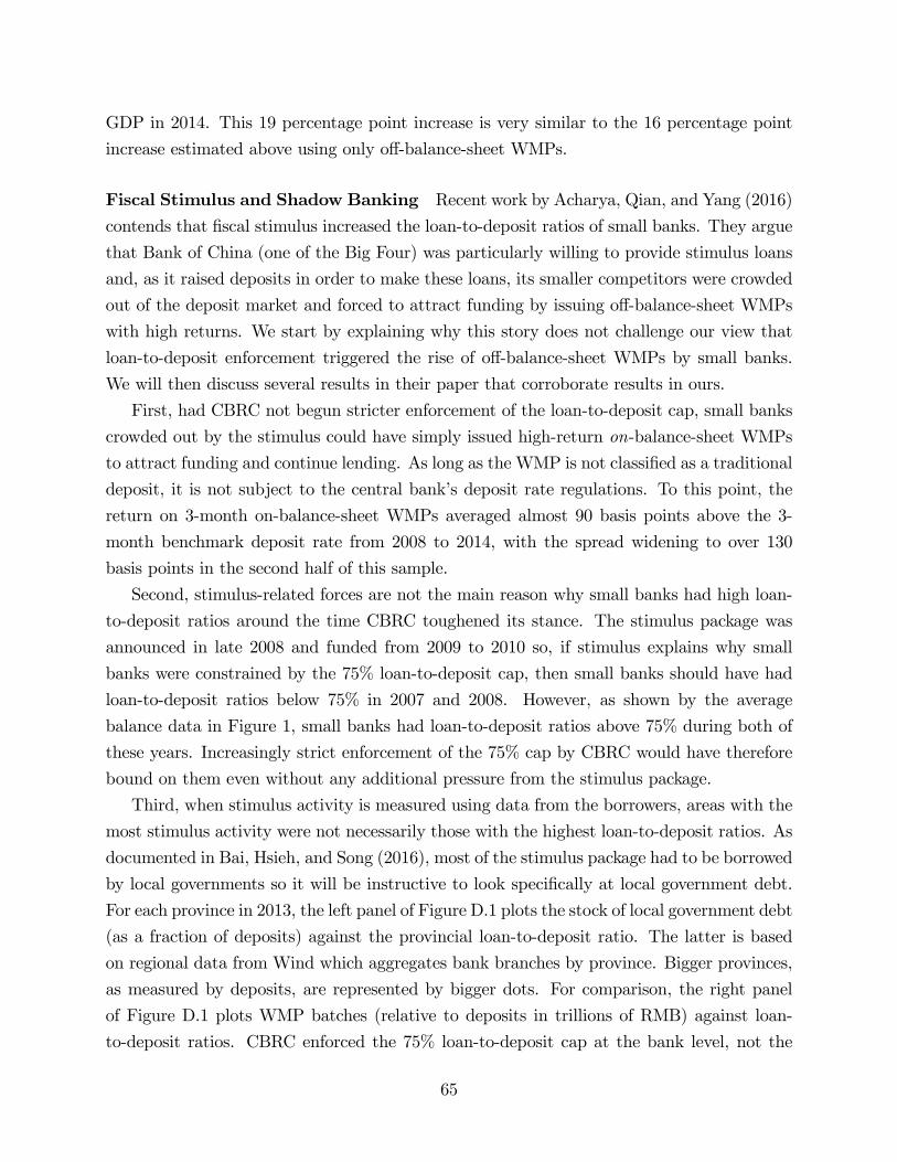
GDP in 2014. This 19 percentage point increase is very similar to the 16 percentage point

increase estimated above using only off-balance-sheet WMPs.

Fiscal Stimulus and Shadow Banking Recent work by Acharya, Qian, and Yang (2016)

contends that fiscal stimulus increased the loan-to-deposit ratios of small banks. They argue

that Bank of China (one of the Big Four) was particularly willing to provide stimulus loans

and, as it raised deposits in order to make these loans, its smaller competitors were crowded

out of the deposit market and forced to attract funding by issuing off-balance-sheet WMPs

with high returns. We start by explaining why this story does not challenge our view that

loan-to-deposit enforcement triggered the rise of off-balance-sheet WMPs by small banks.

We will then discuss several results in their paper that corroborate results in ours.

First, had CBRC not begun stricter enforcement of the loan-to-deposit cap, small banks

crowded out by the stimulus could have simply issued high-return on-balance-sheet WMPs

to attract funding and continue lending. As long as the WMP is not classified as a traditional

deposit, it is not subject to the central bank’s deposit rate regulations. To this point, the

return on 3-month on-balance-sheet WMPs averaged almost 90 basis points above the 3-

month benchmark deposit rate from 2008 to 2014, with the spread widening to over 130

basis points in the second half of this sample.

Second, stimulus-related forces are not the main reason why small banks had high loan-

to-deposit ratios around the time CBRC toughened its stance. The stimulus package was

announced in late 2008 and funded from 2009 to 2010 so, if stimulus explains why small

banks were constrained by the 75% loan-to-deposit cap, then small banks should have had

loan-to-deposit ratios below 75% in 2007 and 2008. However, as shown by the average

balance data in Figure 1, small banks had loan-to-deposit ratios above 75% during both of

these years. Increasingly strict enforcement of the 75% cap by CBRC would have therefore

bound on them even without any additional pressure from the stimulus package.

Third, when stimulus activity is measured using data from the borrowers, areas with the

most stimulus activity were not necessarily those with the highest loan-to-deposit ratios. As

documented in Bai, Hsieh, and Song (2016), most of the stimulus package had to be borrowed

by local governments so it will be instructive to look specifically at local government debt.

For each province in 2013, the left panel of Figure D.1 plots the stock of local government debt

(as a fraction of deposits) against the provincial loan-to-deposit ratio. The latter is based

on regional data from Wind which aggregates bank branches by province. Bigger provinces,

as measured by deposits, are represented by bigger dots. For comparison, the right panel

of Figure D.1 plots WMP batches (relative to deposits in trillions of RMB) against loan-

to-deposit ratios. CBRC enforced the 75% loan-to-deposit cap at the bank level, not the

65

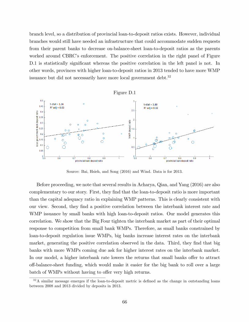
branch level, so a distribution of provincial loan-to-deposit ratios exists. However, individual

branches would still have needed an infrastructure that could accommodate sudden requests

from their parent banks to decrease on-balance-sheet loan-to-deposit ratios as the parents

worked around CBRC’s enforcement. The positive correlation in the right panel of Figure

D.1 is statistically significant whereas the positive correlation in the left panel is not. In

other words, provinces with higher loan-to-deposit ratios in 2013 tended to have more WMP

issuance but did not necessarily have more local government debt.32

Figure D.1

Source: Bai, Hsieh, and Song (2016) and Wind. Data is for 2013.

Before proceeding, we note that several results in Acharya, Qian, and Yang (2016) are also

complementary to our story. First, they find that the loan-to-deposit ratio is more important

than the capital adequacy ratio in explaining WMP patterns. This is clearly consistent with

our view. Second, they find a positive correlation between the interbank interest rate and

WMP issuance by small banks with high loan-to-deposit ratios. Our model generates this

correlation. We show that the Big Four tighten the interbank market as part of their optimal

response to competition from small bank WMPs. Therefore, as small banks constrained by

loan-to-deposit regulation issue WMPs, big banks increase interest rates on the interbank

market, generating the positive correlation observed in the data. Third, they find that big

banks with more WMPs coming due ask for higher interest rates on the interbank market.

In our model, a higher interbank rate lowers the returns that small banks offer to attract

off-balance-sheet funding, which would make it easier for the big bank to roll over a large

batch of WMPs without having to offer very high returns.

32A similar message emerges if the loan-to-deposit metric is defined as the change in outstanding loansbetween 2008 and 2013 divided by deposits in 2013.

66

Monetary Policy and Shadow Banking Recent work by Chen, Ren, and Zha (2016)

contends that shadow banking in China involves small banks using securities called accounts

receivable investments (ARIs) to bring entrusted loans on balance sheet. The authors at-

tribute the rise of ARIs to monetary tightening which they define as lower M2 growth. In the

quantitative analysis of Section 5.3, we find that shocks to liquidity regulation, distinct from

shocks to the supply of liquidity by the central bank, play the dominant role in explaining

the comovement of key interest rates in China, namely the interbank interest rate and the

returns on WMPs.

It is also important to note that small banks held negligible amounts of ARIs prior to

2012. The rise of ARIs was thus predated by the rise of off-balance-sheet WMPs which, as

explained earlier in this appendix, constitute shadow banking. Our paper thus tackles the

foundations of China’s shadow banking system.

In fact, once these foundations are understood, the use of ARIs after 2012 follows quite

naturally from the ideas in our paper.33 In March 2013, CBRC announced that WMPs could

invest at most 35% in non-standard debt assets (e.g., trust assets). Banks using off-balance-

sheet WMPs to circumvent liquidity regulation thus needed to find a less direct way to funnel

WMP money into trust companies. The result was the counterpart business illustrated in

Figure D.2. In short, money is channeled fromWMPs to trusts in two individually compliant

steps. The WMP issuer first places WMP money in another bank (or bank-affi liated off-

balance-sheet vehicle) which we will call Bank B. The WMP’s return is tied to interest

earned on this placement so the WMP is said to be backed by interest rate products, not

trust assets. However, trust companies appear in the next step. In particular, they issue

trust beneficiary rights (TBRs) to Bank B who then uses the cash flows from those rights

to pay the placement interest. Balance sheet data indicate that banks report TBR holdings

either as an investment receivable (ARI) or as collateral in an “offl ine” reverse repo.34 In

other words, ARIs are part of the accounting maneuvers used by banks and trusts in response

to CBRC’s crackdown on direct bank-trust cooperation. At least part of the rise of ARIs

after 2012 was therefore a continuation of the regulatory arbitrage that led to the rise of

off-balance sheet WMPs before 2012.33The explanations that follow extend a discussion in our early draft, “The Rise of China’s Shadow Banking

System,”2015.34Offl ine transactions are ones which do not go through the China Foreign Exchange Trade System.

67

Figure D.2

Business with Counterparts

Notes: TBR stands for trust beneficiary right; SPV is an off-balance-sheet vehicle

Figure D.3 reveals that the counterpart business just described is being facilitated by small

banks. Specifically, the role of Bank B in Figure D.2 is played by joint-stock banks, not by

banks in the Big Four. This helps explain the prevalence of ARIs on small bank balance

sheets. Figure D.3 shows a dramatic rise in TBR holdings among joint-stock banks when

CBRC cracked down on direct bank-trust cooperation in 2013. There was no similar rise

in TBR holdings among the Big Four. Figure D.3 also shows that the joint-stock banks

accommodated their increase in TBR holdings by keeping fewer balances at banks and other

financial institutions (dashed black line). In other words, the JSCBs did not sacrifice loans in

order to hold TBRs. The JSCBs’substitution away from balances at banks is also visible in

the blue bars in Figure D.3: both the JSCBs and the Big Four have experienced decreases in

balances owed to banks. However, unlike the Big Four, the JSCBs have attracted suffi ciently

more balances from non-bank financial institutions (red bars). Off-balance-sheet vehicles that

hold unguaranteed WMPs would be classified as non-bank financial institutions. Effectively,

the off-balance-sheet vehicle of one JSCB places money with another JSCB. The other JSCB

then uses returns from its TBR holdings to pay interest on the placement. This is exactly

the counterpart business illustrated in Figure D.2. In principle, even more counterpart

business could be occurring between the vehicles themselves (e.g., vehicles can hold TBRs

and placements can occur between vehicles).

68

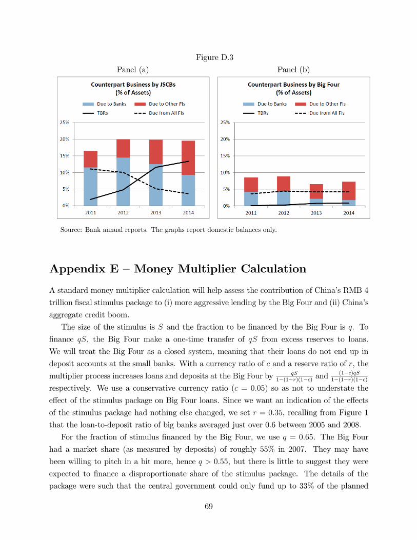
Figure D.3

Panel (a) Panel (b)

Source: Bank annual reports. The graphs report domestic balances only.

Appendix E —Money Multiplier Calculation

A standard money multiplier calculation will help assess the contribution of China’s RMB 4

trillion fiscal stimulus package to (i) more aggressive lending by the Big Four and (ii) China’s

aggregate credit boom.

The size of the stimulus is S and the fraction to be financed by the Big Four is q. To

finance qS, the Big Four make a one-time transfer of qS from excess reserves to loans.

We will treat the Big Four as a closed system, meaning that their loans do not end up in

deposit accounts at the small banks. With a currency ratio of c and a reserve ratio of r, the

multiplier process increases loans and deposits at the Big Four by qS1−(1−r)(1−c) and

(1−c)qS1−(1−r)(1−c)

respectively. We use a conservative currency ratio (c = 0.05) so as not to understate the

effect of the stimulus package on Big Four loans. Since we want an indication of the effects

of the stimulus package had nothing else changed, we set r = 0.35, recalling from Figure 1

that the loan-to-deposit ratio of big banks averaged just over 0.6 between 2005 and 2008.

For the fraction of stimulus financed by the Big Four, we use q = 0.65. The Big Four

had a market share (as measured by deposits) of roughly 55% in 2007. They may have

been willing to pitch in a bit more, hence q > 0.55, but there is little to suggest they were

expected to finance a disproportionate share of the stimulus package. The details of the

package were such that the central government could only fund up to 33% of the planned

69

investment/expenditure. The rest of the funds were to be borrowed by local governments.

In modern-day China, the central government exercises only indirect control over the Big

Four (e.g., through top personnel decisions) and can exercise exactly the same control over

the JSCBs since they also operate nationally. Local governments have no administrative

control over commercial banks. Their only leverage is economic (e.g., where to put local

government savings) and it tends to work better with smaller/locally-operating banks such

as city banks. In short, local governments are simply not powerful enough to force the Big

Four (or even the JSCBs) to lend huge amounts of money that they otherwise would not

have lent. For this reason, the fraction of the stimulus that we attribute to the Big Four is

guided by their market share.

The results of our calculation suggest that China’s stimulus package can account for up

to RMB 6.8 trillion of new loans and up to RMB 6.5 trillion of new deposits at the Big Four

since the end of 2008. Taking these amounts out, loans and deposits at the Big Four would

have grown at annualized rates of 12.9% and 9.8% respectively from 2008 to 2014. The Big

Four’s loan-to-deposit ratio would have then increased from 0.57 in 2008 to 0.67 in 2014.

This counterfactual estimate of what would have happened to the Big Four’s loan-to-deposit

ratio absent stimulus is similar to what actually happened with the stimulus (an increase

from 0.57 in 2008 to 0.70 in 2014 as per Figure 1).

We now extend the calculation to estimate how much of the overall increase in China’s

credit-to-savings ratio can be reasonably explained by stimulus alone. Suppose the remaining

(1− q)S of stimulus was financed by small banks. This amount will also go through themultiplier process, except with a lower reserve ratio (call it r) since small banks have higher

loan-to-deposit ratios than the Big Four. We set r = 0.15 based on the average balance data

for 2007 in Figure 1. Combining the calculations for the small banks with the calculations

for the Big Four, we find that the stimulus package explains around 40% of the 10 percentage

point increase in China’s credit-to-savings ratio since 2007.

Appendix F —Estimation Procedure

Let m = 1, ..., 6 index the empirical moments to be matched. The six moments are the six

correlations in Table 2.

1. Bootstrap: Let N denote the total number of random samples generated by bootstrap.

We set N = 500. Denote by gm,n the mth moment in the nth sample. We will target1N

∑Nn gm,n, the m

th moment averaged across N samples.

70

2. Denote by Ω the vector of parameters to be estimated. Given Ω, we can simulate the

model to generate the moments gm (Ω). Denote by εm,n = gm (Ω) − gm,n the residualfor moment m in sample n. Define the weighting matrix (M ×M) as:

W =1

N

N∑n

εm,nεTm,n

3. Minimizing the weighted sum of the distance between the empirical and simulated

moments:

Ω = arg minΩh (Ω)′W−1h (Ω)

where h (Ω) is a vector with M elements and hm (Ω) = gm (Ω)− 1N

∑Nn gm,n.

4. We use two-step Simulated Method of Moments. We set W to the identity matrix in

the first step and useW from the first-step as the weighting matrix for the second-step

estimation.

5. Repeat the above exercise 100 times to calculate the standard errors of the estimated

parameters.

71