liquidity in the german corporate bond market: has the

Discussion PaperDeutsche BundesbankNo 08/2021

Liquidity in the German corporate bond market:has the CSPP made a difference?

Lena Boneva(European Central Bank and CEPR)

Mevlud Islami(Deutsche Bundesbank)

Kathi Schlepper(Deutsche Bundesbank)

Discussion Papers represent the authors‘ personal opinions and do notnecessarily reflect the views of the Deutsche Bundesbank or the Eurosystem.

Editorial Board: Daniel Foos Stephan Jank Thomas Kick Malte Knüppel Vivien Lewis Christoph Memmel Panagiota Tzamourani

Deutsche Bundesbank, Wilhelm-Epstein-Straße 14, 60431 Frankfurt am Main, Postfach 10 06 02, 60006 Frankfurt am Main

Tel +49 69 9566-0

Please address all orders in writing to: Deutsche Bundesbank, Press and Public Relations Division, at the above address or via fax +49 69 9566-3077

Internet http://www.bundesbank.de

Reproduction permitted only if source is stated.

ISBN 978–3–95729–816–4 (Internetversion)

Non-technical summary Research question The Eurosystem purchased €178 bn of corporate bonds between June 2016 and December 2018 during the Corporate Sector Purchase Programme (CSPP). Did these purchases ad-versely affect liquidity conditions in the corporate bond market, thus raising concerns about unintended consequences of large-scale asset purchases? Our results suggest that purchases conducted under the CSPP have led to an improvement of liquidity conditions in the short run. In the long run, however, CSPP purchases might have deteriorated liquidity to some extent. Contribution To analyse the impact of CSPP purchases on market liquidity in the market for German cor-porate bonds, we combine the Bundesbank's detailed CSPP purchase records with a range of liquidity indicators. We assess both ``flow'' and ``stock'' effects of the purchases, where flow effects measure the contemporaneous impact of the Bundesbank's purchases on market li-quidity. In contrast, stock effects measure the accumulated impact of the purchases on liquidity conditions prevailing in the German corporate bond market after the end of CSPP net pur-chases in December 2018 compared to before these purchases had begun. In addition, the granularity of our dataset allows us to explore how the effect of CSPP purchases on market liquidity varies across market conditions and bond characteristics. Assessing the impact of CSPP purchases on market liquidity can improve our understanding of the transmission mechanism of unconventional monetary policies. In particular, liquidity premia are often mentioned in addition to duration or local supply effects as one channel through which corporate bond purchases affect corporate bond yields. Results We find that initially, the Bundesbank's corporate bond purchases improved contemporaneous liquidity conditions in the market for German corporate bonds (flow effect) albeit the estimated effects are relatively small. For an average purchase size of €7m, bid-ask spreads of pur-chased bonds tightened by 0.7bps on the day of the purchase. However, liquidity conditions deteriorated as the Bundesbank reduced the stock of corporate bonds available for trading in the secondary market (stock effect). For the average volume purchased by bond over the life-time of the CSPP (€29m), we find that the bid-ask spread increased by around 1 bps. The results of our analysis also show that the liquidity of old (and already illiquid) bonds has deteriorated in the short- and long-run while it has improved for newly issued bonds.

Nichttechnische Zusammenfassung Fragestellung Im Rahmen des Corporate Sector Purchase Programme (CSPP) hat das Eurosystem im Zeit-raum zwischen Juni 2016 und Dezember 2018 Unternehmensanleihen im Wert von €178 Mrd angekauft. Dabei stellt sich die Frage, ob diese großen Ankäufe die Liquidität am Markt für Unternehmensanleihen verschlechtert haben? Die Ergebnisse dieser Studie legen eine kurz-fristige Verbesserung der Liquidität nahe. Langfristig führen die Anleihekäufe hingegen zu ei-ner Verschlechterung der Liquidität. Beitrag In dieser Studie verwenden wir einen granularen Datensatz von der Deutschen Bundesbank zu den im Rahmen des CSPP angekauften Anleihen in Kombination mit einer Reihe von Li-quiditätsmaßen, um den Einfluss von Anleihekäufen auf die Marktliquidität zu analysieren. Wir schätzen sowohl den „Flow-“ als auch den „Stock“-Effekt der Anleihekäufe, wobei der Flow-Effekt den zeitgleichen Effekt der Anleihekäufe auf die Marktliquidität misst. Der Stock-Effekt hingegen misst den kumulierten Effekt der Anleihekäufe auf die Liquidität zwischen dem Be-ginn und dem Ende der Netto-Anleihekäufe. Aufgrund der Granularität des Datensatzes kön-nen wir untersuchen, wie Anleihekäufe die Marktliquidität in Abhängigkeit von Marktbedingun-gen und Anleihecharakteristika beeinflussen. Eine Bewertung des CSPP-Einflusses auf die Marktliquidität kann dazu beitragen, das Ver-ständnis des Transmissionsmechanismus unkonventioneller Geldpolitik zu verstehen. Der Einfluss der Anleihekäufe auf die Renditen von Unternehmensanleihen wird gemäß Literatur insbesondere über die Liquiditätsprämie und Duration einer Unternehmensanleihe sowie durch lokale Angebotseffekte transportiert. Ergebnisse Die Ergebnisse unserer Studie zeigen, dass die Ankäufe von Unternehmensanleihen die Li-quidität am deutschen Unternehmensanleihemarkt kurzfristig verbessert haben (Flow-Effekt), wobei die geschätzten Effekte vergleichsweise klein sind. So verringerten sich die Geld-Brief-Spannen bei einem durchschnittlichen Ankaufsvolumen von €7 Mio um 0.7 Basispunkte am Tag der Anleihekäufe. Die Liquiditätsbedingungen verschlechterten sich jedoch nach dem Ende der Netto-Anleihekäufe, da sich das am Sekundärmarkt verfügbare Handelsvolumen re-duzierte (Stock-Effekt). Bei einem über die gesamte Laufzeit des CSPP durchschnittlichen An-kaufsvolumen pro Anleihe in Höhe von €29 Mio stieg z.B. die Geld-Briefspanne um 1 Basis-punkt. Die Ergebnisse unserer Analyse zeigen auch, dass sich die Liquidität von älteren und ohnehin illiquiden Anleihen sowohl kurz- als auch langfristig verschlechtert hat. Hingegen hat sich die Liquidität kürzlich emittierter und vergleichsweise liquider Anleihen verbessert.

Lena Boneva† Mevlud Islami‡ Kathi Schlepper§

∗We would like to thank Emanuel Monch, Christiane Sack, Bernd Wiesemann, Holger Spies, Clemens

Werner, Andreas Moser, Bernd Struber, Heiko Hofer, Martin Wieland and Marco Leppin for their helpful

comments and contributions.†European Central Bank and CEPR. Email: Lena [email protected]‡Deutsche Bundesbank, DG Financial Stability. Email: [email protected]§Deutsche Bundesbank, DG Markets. Email: [email protected]

Bundesbank Discussion Paper No 08/2021

Liquidity in the German corporate bond market: has

the CSPP made a difference?∗

March 9, 2021

Abstract

The Eurosystem purchased e178 billion of corporate bonds between June 2016 and December 2018 under the Corporate Sector Purchase Programme (CSPP). Did these purchases lead to a deterioration of liquidity conditions in the corporate bond market, thus raising concerns about unintended consequences of large-scale asset purchases? To answer this question, we combine the Bundesbank’s detailed CSPP purchase records with a range of liquidity indicators for both purchased and non-

purchased bonds. We find that while the flow of purchases supported secondary market liquidity, liquidity conditions deteriorated in the long-run as the Bundes-

bank reduced the stock of corporate bonds available for trading in the secondary

market.

Keywords:Corporate Bond Market, Central Bank Asset Purchases, Market Liquidity

JEL classification: E52, F30, G12

1 Introduction

In 2016, the Eurosystem launched the Corporate Sector Purchase Programme (CSPP)

as part of its large-scale Asset Purchase Programme (APP) with the objective to bring

inflation back to levels in line with the ECB’s target. But besides their intended impact on

economic activity, central bank asset purchases are likely to also affect market functioning

by providing a predictable source of demand for bonds, for example. Because of this

’back-stop’ buyer effect, dealers are more willing to hold larger inventories to facilitate

market-making. In addition, asset purchases can stimulate trading activity as dealers

are likely to purchase another bond after selling one to the Eurosystem. On the other

hand, asset purchases can also lead to a deterioration of market liquidity in particular

if the purchase programme is relative large. If a large proportion of corporate bonds is

held by the Eurosystem, sourcing a particular bond can become more costly for dealers

(Ferdinandusse, Freier, and Ristiniemi (2017)).

In view of these ambiguous predictions, this paper estimates the impact of CSPP

purchases on market liquidity in the market for German corporate bonds using a granular

dataset of the Bundesbank’s individual CSPP purchases. We assess both “flow” and

“stock” effects of the purchases, where flow effects measure the contemporaneous impact

of the Bundesbank’s purchases on market liquidity. In contrast, stock effects measure the

accumulated impact of the purchases on liquidity conditions prevailing in the German

corporate bond market after the end of CSPP net purchases in December 2018 compared

to before these purchases had begun. In addition, the granularity of our dataset allows

us to explore how these effects of CSPP purchases on market liquidity vary across market

conditions and bond characteristics.

Identification of flow effects of central bank asset purchases on liquidity is inherently

difficult (Boneva, Elliott, Kaminska, Linton, McLaren, and Morley (2018)). Specifically,

the impact of purchases on liquidity is likely to be confounded by reverse causality that

arises if, for example, financial institutions prefer to sell more illiquid bonds to the central

bank that are more difficult to sell in secondary markets. Also, reversed causality is a

concern if liquidity considerations play a role in the purchasing decision of the central

bank due to risk management considerations, for example. We follow Boneva, Elliott,

Kaminska, Linton, McLaren, and Morley (2018) and tackle these identification challenges

by using our granular dataset containing a wide range of information about the purchase

process to construct proxies for supply and demand to control for reverse causality.

We find that initially, the Bundesbank’s corporate bond purchases improved contempo-

raneous liquidity conditions in the market for German corporate bonds (flow effect) albeit

the estimated effects are relatively small. For an average purchase size of e7m, bid-ask

spreads of purchased bonds tightened by 0.7bps on the day of the purchase compared to

1

an average bid-ask spread of 35bps and trading volume increased by e0.6m compared to

an average of 2.5 for purchased bonds. However, liquidity conditions deteriorated as the

Bundesbank reduced the stock of corporate bonds available for trading in the secondary

market (stock effect). This is particularly true for the resilience measures studied. For

the average volume purchased by bond over the lifetime of the CSPP (e29m), we find

that the number of quotes received for a purchased bond compared to a not purchased

bond fell by around 2.2 and the number of dealers quoting the bond fell by around 0.3,

compared to their averages of 137 and 12, respectively. These findings are consistent with

Ferdinandusse, Freier, and Ristiniemi (2017) who develop a search-theoretic framework

to study the impact of asset purchases by central banks on prices and liquidity. In line

with our results, their model predicts that liquidity improves initially as the central bank

constitutes another large player in the market that stands ready to buy. After the end of

the central bank purchases, their model predicts that liquidity is worse than before the

start of the purchases because of the lower free-float available for private investors.

The purchases were carried out both during tranquil periods and periods of height-

ened market volatility. For example, the UKs vote to leave the EU, the Italian elections

in early 2018, and the US-China trade war all took place during the purchase period. In

addition, the eligibility criteria for the CSPP are relatively broad, covering bonds with a

wide range of different characteristics. One reason for this broad approach is the concept

of market neutrality underlying the CSPP implementation aiming at minimizing potential

unintended side effects on market functioning. Therefore, we also assess how the impact

of the purchases varied across market conditions and bond characteristics. Considering

the flow effect, for example, CSPP purchases tightened bid-ask spreads for a bond with

an average age of around 3 but bid-ask spreads widen instead for bonds with an age of 4.7

and older. One explanation for this result could be that bonds are traded more frequently

when newly issued. As they age, bonds are traded less frequently as a significant portion

is purchased by buy-and-hold investors who reduce the free float available for trading by

other investors (Mahanti, Nashikkar, Subrahmanyam, Chacko, and Mallik (2008)). Thus,

central bank purchases of old bonds may reduce their liquidity further. Moreover, this

could imply that the CSPP has mainly improved the liquidity of already more liquid

bonds, thereby potentially favouring a “bifurcation” of corporate bond liquidity. Regard-

ing the stock effect, the CSPP impact also seems to depend strongly on age. For example,

the Amihud illiquidity measure increases for an average age of 2 years, and the number

of quotes increases for bonds since issuance.

These findings add to our understanding of the transmission mechanism of unconven-

tional monetary policies. In particular, liquidity premia are often mentioned in addition

to duration or local supply effects as one channel through which corporate bond purchases

2

affect corporate bond yields. Our results provide evidence that central bank purchases of

corporate bonds can affect these premia both in the short- and long run.

There is a growing literature that assesses the impact of central bank asset purchases

of sovereign bonds on secondary market liquidity, often reaching contrasting results. For

example, Eser and Schwaab (2011), De Pooter, Martin, and Pruitt (2018) and Steeley

(2015) find that government bond purchases improved liquidity while Han and Senevi-

ratne (2018) and Kurosaki, Kumano, Okabe, and Nagano (2015) find that the Bank of

Japan’s sovereign bond purchases damaged liquidity. Some papers find mixed evidence

within a single purchase programme, including Schlepper, Hofer, Riordan, and Schrimpf

(2020), Pelizzon, Subrahmanyam, Tobe, and Uno (2018), Christensen and Gillan (2018)

and Iwatsubo and Taishi (2016). In part, these contrasting results are perhaps due to

differences in purchase size and design across countries, consistent with Ferdinandusse,

Freier, and Ristiniemi (2017). Also, the period when as asset purchase programme is

carried out and the length of its application play an important role. Accordingly, central

banks purchases tended to improve market functioning particularly in markets with high

liquidity premia including those experiencing periods of stress and for less liquid securities

such as private sector assets or off-the-run government securities. A case in point are Eser

and Schwaab (2011), De Pooter, Martin, and Pruitt (2018) who analyze the effects of

the SMP programme in different euro area bond markets during the euro debt crisis and

find a positive effect. On the other hand, declines in market making and reduced investor

participation have occurred in some markets, in particular where policies were in place

for an extended period of time (BIS Markets Committee (2019)).

Compared to sovereign bonds, the literature on the impact of non-sovereign bond

purchases on liquidity is still relatively scarce. Exceptions include Kandrac (2013) and

Kandrac (2018) who find that the Federal Reserve’s MBS purchases damaged liquidity

in these markets. In contrast, Todorov (2018) finds that liquidity of CSPP-eligible bonds

increased at the announcement of the scheme. Also, Beirne, Dalitz, Ejsing, Grothe, Man-

ganelli, Monar, Sahel, Susec, Tapking, and Vong (2011) find positive effects of the Eu-

rosystem’s covered bond purchase scheme on market liquidity and covered bond spreads.

In addition, Boneva, Elliott, Kaminska, Linton, McLaren, and Morley (2018) document

that Bank of England’s corporate bond purchases improved market liquidity in the Ster-

ling corporate bond market just after the purchases took place, but do not detect any

longer term effect of these purchases. They pioneered the use of granular data from central

bank purchase operations to tackle reversed causality issues and our paper follows their

approach. Using a similar methodology, we also find a positive effect of central bank pur-

chases in the short-run. But our results for the long-run effect of central bank corporate

bond purchases on liquidity in the German corporate bond market contrast sharply with

3

those for the sterling market. In particular, we present evidence for sizable longer term

or stock effects from the Bundesbank’s CSPP purchases while Boneva, Elliott, Kaminska,

Linton, McLaren, and Morley (2018) do not detect any longer term impact in case of

the Bank of England’s CBPS purchases. We attribute this difference to the difference in

the overall amount purchased relative to the size of the eligible universe. The Bank of

England purchased only 5% of eligible Sterling corporate bonds (Belsham, Maher, and

Rattan (2017 Q3)) while the corresponding number for the Eurosystem’s corporate bond

purchases is much larger with around 16%1.

Finally, there is also a range of papers examining the impact of the CSPP on corpo-

rate bond spreads and issuance of euro-denominated corporate bonds (De Santis, Geis,

Juskaite, and Vaz Cruz (2018), Hammermann, Leonard, Nardelli, and von Landesberger

(2019), Zaghini (2017), Arce, Gimeno, and Mayordomo (2017), Grosse Rueschkamp, Stef-

fen, and Streitz (2019) and Abidi and Miquel Flores (2018)). In contrast to their work,

we study the CSPP through the lens of a granular dataset containing information about

the purchase process to tackle the identification challenges discussed above.

The remainder of this paper is organized as follows. Section 2 provides an overview of

the CSPP and how the purchases at the Bundesbank are carried out which informs our

identification strategy. Section 3 introduces both the data on the Bundesbank’s CSPP

purchases and our liquidity measures for the German corporate bond market. Section 4

studies flow effects by relating CSPP purchases to contemporaneous liquidity conditions

prevailing in the German corporate bond market. Section 5 examines the longer term or

so-called stock effects of the Bundesbank’s CSPP purchases on market liquidity. Section

6 concludes.

2 The ECB’s Corporate Sector Purchase Programme:

overview and design

2.1 Overview

The ECB announced its Corporate Sector Purchase Programme in March 2016 against

a backdrop of deflationary pressure and headwinds to growth in order to ease financing

conditions in the euro area, hence supporting investment and growth and facilitating the

return of euro area inflation to its target level to below, but close to, 2 percent over the

medium term.

The CSPP was part of a broader set of policy measures that were introduced in order

1This figure also broadly represents the individual National Central Banks’ share of CSPP purchases

relative to the eligible universe of the respective corporate bond market.

4

to achieve the price stability target of the Eurosystem: (i) a cut in key ECB interest rates;

(ii) a new series of four targeted longer-term refinancing operations and (iii) an increase

in the monthly net sovereign bond purchases under the APP from e60 billion to e80

billion.

Eligibility criteria for the CSPP are broad-based and cover a wide range of euro-

denominated bonds that are issued by euro area non-bank corporations. Specifically,

corporate bonds are eligible for the CSPP if they fulfill the following criteria (ECB (2016)):

they are eligible as collateral for Eurosystem credit operations; they are denominated in

euro; they have a minimum first-best credit assessment of at least BBB- or equivalent

obtained from an external credit assessment institution; they have a minimum remaining

maturity of six months and a maximum remaining maturity of 30 years at the time of

purchase; the issuer is a corporation established in the euro area, defined as the location of

incorporation of the issuer2 and not exceed the upper bound on the Eurosystem’s holdings

of 70 percent per security3. Corporate bonds issued by credit institutions, institutions with

a parent qualifying as a credit institution, asset management vehicles, or national asset

management and divestment funds established to support financial sector restructuring

and/or resolution are not eligible for purchases under the CSPP.

CSPP purchases started on 8 June 2016 and took place in both the primary and

secondary market, and were implemented by the Bundesbank, Banque de France, Banca

D’Italia, Banco de Espana, Suomen Pankki, and Banque Nationale de Belgique on behalf

of the Eurosystem. In terms of efficiency, the Eurosystem decided that not all 19 national

central banks (NCB) and the ECB carry out the purchases, also due to a very small

universe of the corporate bond markets in some jurisdictions. National central banks

had some discretion regarding how to implement the purchases operationally while the

Eurosystem coordinated the purchases by establishing a common set of eligibility criteria

and setting the overall amount to be purchased by each NCB in a particular month.

An important criterion guiding the CSPP purchases is market neutrality aimed at

minimizing the impact on relative prices within the eligible universe and potential un-

intended side effects on market functioning (Hammermann, Leonard, Nardelli, and von

Landesberger (2019)). For the CSPP, market neutrality implies that NCBs participating

in the purchases aimed at keeping their holdings by issuer and sector as close as possible

to their respective market shares in the eligible universe of the respective corporate bond

market. To further limit negative effects on market functioning, CSPP holdings are avail-

2Corporate debt instruments issued by corporations incorporated in the euro area whose ultimate

parent is not based in the euro area are also eligible for purchase under the CSPP, provided they fulfill

all the other eligibility criteria.3The threshold of 70 percent is applied to bonds issued by private corporations and is lower for public

issuers.

5

able for securities lending by the relevant purchasing national central banks, who publish

a list of the individual bonds they hold on a weekly basis without revealing the size of

their holdings in each bond.

In December 2018, the ECB’s Governing Council announced to end net asset purchases

under the asset purchase programme that also includes the CSPP, while continuing to

reinvest principal payments from maturing securities purchased. But purchases under

the APP were restarted as of November 2019 against a backdrop of muted inflationary

pressure and weakness of the euro area economy.

During the initial phase of the APP (2015-2018), the total purchase volume has been

adjusted several times until net purchases have ended in December 2018. With this

gradual reduction the CSPP purchase volume has also declined, although by less in relative

terms compared to the Public Sector Purchase Programme (PSPP).

2.2 The Bundesbank’s CSPP purchases

The Bundesbank purchases eligible corporate bonds both on the secondary and primary

market, with the former constituting the majority of its purchases. To purchase corporate

bonds from the secondary market, the Bundesbank collects individual dealer’s offers of

eligible ISINs obtained via email on a regular, usually daily, basis. The decision of which

eligible bond to purchase depends on different factors. One factor is market neutrality

that requires the Bundesbank to keep its holdings by issuer as close as possible to their

market shares in the universe of eligible collateral for tender operations. Other relevant

factors include the offered volume and the monthly volume target provided by the ECB.

All factors are equally important.

After the ISINs to be purchased are chosen, the Bundesbank usually sends request for

quotes (RFQ) to those dealers who clearly display their inventories in the respective ISIN

to the Bundesbank or who are known to be active in this particular bond segment. In rare

occasions, the Bundesbank contacts the dealers directly through chat or phone to request

their prices and to trade with the dealer. The Bundesbank decides about the quantity to

purchase based on its monthly volume targets provided by the ECB. One bond may be

purchased more than once per day.

The Bundesbank also buys a certain amount of bonds on the primary market. Between

January 2017 and October 2018 the Bundesbank participated in several corporate bond

auctions of non-public owned companies. Among all 51 issuers, 6 issuers are public which

is why these bonds cannot be purchased on the primary market, i.e. due to the restriction

of “no monetary financing of the public sector”.

6

3 Data

3.1 Purchase data

While the Bundesbank purchases bonds both on the primary and on the secondary market,

we only use secondary market purchases as they can be directly linked to the secondary

market liquidity that is the focus of our paper.4

Figure 1 shows the aggregate monthly purchase volume splitted by sectors (in em).

The highest share of purchases by the Bundesbank is carried out for the consumer cyclicals

sector, although the relative shares vary also over time. The financial sector refers to

insurance companies and real estate, banks are excluded.

Table 1 and Figure 2 report descriptive statistics for both the RFQ process and pur-

chases for all secondary market transactions. On a typical day, the Bundesbank sends

a RFQ to 22 different dealers for each bond it is interested in purchasing. These RFQs

are usually sent via two different trading systems. The RFQ process is carried out for on

average 8 different bonds per day. However, this number varies strongly over time in a

range between 1 and 24, probably also dependent on Bundesbank’s specific volume tar-

gets. The offered volume by bond is around e76m on average. Turning to the purchases,

each bond is purchased on average 2.5 times per day. The average purchase size is around

e3m but exhibits a relatively high volatility as well. The overall traded volume by bond

varies relatively strongly, too: while the average is around e7m, there are cases when no

trade occurs at all and transactions with high volumes of up to e262m. This suggests that

the trades indeed may depend on quantities offered and on market conditions. Finally,

the coverage ratio is calculated by dividing the overall volume purchased of a specific

bond by the total volume offered in the RFQ process. It is on average 0.10, meaning that

the Bundesbank roughly purchases 10% of what the banks offer. Figure 2 shows that

most of these RFQ and trade statistics are nearly equally spread over maturity buckets.

While more trades are carried out in the small bucket of 0-3 years residual maturity, more

volume has been purchased at larger ticket size in the large maturity bucket (> 7 years

residual maturity).

Table 2 provides more detailed information on the frequency of the Bundesbank’s

CSPP purchases. In around 4% of all trading days, no transaction occurred. One reason

for why this can happen is that the prices offered by dealers are too unattractive. Another

4Our RFQ and trade dataset doesn’t contain any identification of primary purchases which is why we

have to apply different criteria obtained from Bundesbank portfolio managers to exclude them. Primary

purchase data is excluded by dropping (1) all purchases larger than e10m, and (2) all purchases that

take place within the first 7 days after bond issuance. Usually, the acquisition of corporate bonds on the

primary market takes place via auctions or bilateral purchases on or close to the issuance day and at

large volumes.

7

reason is that there might be too few prices offered to Bundesbank or finally, the difference

to the previous transaction price is too high. In any of these cases, the Bundesbank

rejects the offer and the RFQ process does not result in a trade. The case observed most

frequently is that one or two trades per bond are observed per day. In 90% of the cases,

no more than four and in 99% no more than nine trades take place in a specific ISIN

on a daily frequency. In our study period from the start of the CSPP in June 2016 to

December 2018 overall 362 bonds have been purchased by Bundesbank.

3.2 Liquidity measures

In order to measure liquidity in the German corporate bond market at the individual

bond level, we use daily price-based data (dealer quotes) from Markit and trading activity

data from Euroclear. Overall, our dataset consists of 246 senior unsecured fixed coupon

investment grade (IG) bonds issued by German non-financial corporations, denominated

in euro, with a remaining maturity between one and ten years, a maturity at issuance of at

least 1.5 years and a minimal amount outstanding of e500m. Moreover, the dataset also

includes 28 senior unsecured fixed coupon high yield (HY)bonds issued by German non-

financial corporations, denominated in euro, exhibiting a minimal amount outstanding of

e250m. A bond is classified as HY if its average credit rating is at or below BB+. We

use HY bonds in the subsequent analysis as some of these bonds fulfil the ECB eligibility

criterion of exhibiting a first-best rating of at least BBB- and can thus be purchased under

the CSPP. Furthermore, we use HY ineligible bonds as control group in our analysis in

addition to the baseline group of eligible non-purchased bonds. In our dataset, the non-

financial sector does not include real estate companies and bonds issued by non-bank

financial institutions (such as insurances). Compared to the overall size of the corporate

bond market as measured by our dataset, the German subset comprises around 21% of

the overall IG universe and around 12% of the overall HY universe.

Liquidity is multifaceted and therefore a unique definition does not exist. In general

one can distinguish between four liquidity dimensions, i.e. tightness, immediacy, depth,

and resilience.5 We use the bid-ask spread, i.e. the difference between ask price and bid

price of a bond as a proxy for tightness. This measure can be interpreted as the costs

of executing a trade. The lower the spread the easier a bond should be purchased and

sold and, thus, the better should be the liquidity conditions. As a further measure of

tightness we also employ the effective bid-ask spread proposed by Roll (1984). As Roll

(1984) shows, under certain conditions the effective bid-ask spread corresponds to two

5As a fifth dimension sometimes breadth is used. It implies that in a liquid market big orders should

not have a significant impact on prices. Following the CGFS (2016) we use depth and breadth as one

facet of liquidity.

8

times the square root of the negative first-order autocovariance of returns.

In order to capture immediacy we use the range of high and low prices during a day.

The idea behind it is that in case of poor immediacy, trades cannot easily be executed.

However, once executed price fluctuations are high and, thus, a wide range should be an

indicator of poor immediacy and vice versa (see Broto and Lamas (2016), and Broto and

Lamas (2019)). As a second proxy for immediacy, we employ the variable time to unwind,

defined as the number of days to exit a e5m position. Markit calculates this measure as

e5m divided by the expected daily trading volume. The latter is defined as trades per

day times the average ticket size (in em) over the last 30 days.

Trading volume-based liquidity measures (which have been transformed to daily basis),

i.e. the 30 day trading volume of daily transactions, and the illiquidity measure of Amihud

(2002) have been employed in order to capture the aspect of depth. In general, higher

trading volumes are considered positive from the liquidity perspective, while high price

sensitivity in response of a bond purchase or selling suggests a poor liquidity and vice

versa. Thus, an increase of the Amihud illiquidity measure (defined as the absolute one

day price return (in bps) divided by the trading volume) suggests a deteriorating liquidity

and vice versa.

The aspect of resilience is represented by the liquidity measures average ticket size,

the number of dealers quoting the bond averaged over one business day, and the number

of unique quotes received for an instrument over one business day. High values of these

measures indicate a high liquidity and low values a poor liquidity on the corporate bond

market.6 Table 3 summarizes the liquidity measures employed in this analysis.

Figures 3-6 document that liquidity conditions changed markedly over the period from

early 2015 to early 2019.7 In the period before the announcement of CSPP from the second

half of 2015 to early 2016, financing and liquidity conditions deteriorated significantly

owing to concerns on the growth prospects of China and other large emerging countries,

and weaker than expected US economic data. HY bonds reacted stronger to the increased

volatility, as e.g. indicated by the sharp increase of the Roll measure for HY bonds in

early 2016.

6Notice that we have winsorised liquidity measures at 1% and 99% to reduce the impact of extreme

outliers.7Notice that some regulatory changes during this period could have affected liquidity of corporate

bonds. Regulatory reforms such as Basel III make highly liquid bonds more popular than bonds considered

as less liquid. The liquidity coverage ratio, for example, requires banks to hold a certain ratio of high-

quality assets such as highly rated government and corporate bonds. However, at the same time other

investors have compensated at least partially the declining demand of the banks for other than high-

quality bonds. Moreover, since only a small part of German non-financial corporate bonds exhibits a

high credit quality (i.e. a AA rating or better), the impact of regulatory reforms on the German market

should be rather moderate.

9

The CSPP was announced against the backdrop of receding uncertainty in financial

markets as growth prospects started to improve in early 2016. At this time, the Eu-

rosystem announced the CSPP, thereby leading to an immediate significant decrease in

spreads of eligible corporate bonds as evidenced by De Santis, Geis, Juskaite, and Vaz Cruz

(2018). And Todorov (2018) finds that liquidity of CSPP-eligible bonds increased at the

announcement of the scheme. Over most of the CSPP purchase period from March 2016

to mid-2018, liquidity measures like bid-ask spread, Roll, daily range, Amihud, average

ticket size, the number of dealers, and the number of quotes continued to improve. A

striking feature is that the number of quotes per bond increased extraordinary strong in

2018. A reason for this observation could be the strong issuance activity on the Euro-

pean corporate market during the CSPP purchase period (De Santis, Geis, Juskaite, and

Vaz Cruz (2018)). The other liquidity measures (time to unwind and trading volume)

suggest a slight deterioration or do not allow for a clear conclusion. In the second half of

2018, concerns around a further escalation in the trade dispute between the US and China

caused an increase of risk aversion and thus a deterioration of market liquidity. Moreover,

market liquidity usually declines at the end of the year. The end of net purchases in

December 2018 was widely expected by the market participants and did not trigger a

strong market reaction.

Overall, despite deteriorating conditions in the second half of 2018, liquidity conditions

improved in general after the CSPP announcement as suggested by the comparison of the

liquidity measures’ mean values before and after the announcement of the CSPP (Tables

4-8). However, as discussed above, the CSPP purchases took place at the same time as a

wide range of other events with potentially sizable effects on the German corporate bond

market including the UK’s vote to leave the EU, the Bank of England’s corporate bond

purchases and the US-China trade dispute, among many others. Therefore, we now carry

out an econometric analysis to control for these confounding events and hence to isolate

the impact of CSPP purchases on market liquidity.

4 Flow effects of Bundesbank’s CSPP purchases on

liquidity

We start by estimating the contemporaneous effect of the Bundesbank’s corporate bond

purchases on liquidity. This so-called flow effect of the CSPP offers insights into how

individual purchases affected market functioning in the German corporate bond market

immediately after the purchases are carried out. But estimating these effects is plagued

by reversed causality and the next section explains how we tackle this problem.

10

4.1 Identification

Identifying the impact of purchases on liquidity or prices is difficult because of reverse

causality: in general, dealers take into account liquidity indicators when deciding about

whether or not to sell a bond to an NCB, and NCBs’ purchasing decisions are likely

to depend on liquidity, too.8 To reduce this reverse causality issues, we explore design

features of the Bundesbank’s purchase mechanism, together with detailed data about the

purchases.

As described in Section 2.2 above, the Bundesbank’s purchase decision depends on

market neutrality, dealers’ inventories and the purchase target. While the latter does not

depend on liquidity, liquidity conditions can have an impact on dealers’ inventories if, for

example, dealers are more willing to hold liquid bonds. Liquidity conditions can also affect

by how much the Bundesbank’s holdings deviate from market neutrality if past purchases

depend on liquidity, which is likely to be the case. However, according to Bundesbank’s

trading desk, liquidity considerations don’t play a direct role in their trading approach,

but affect the RFQ process only indirectly. If the Bundesbank sends many requests to

dealers for a specific bond, this is only a consequence of a large number of offers the

Bundesbank portfolio managers receive previously. The more liquid a bond, the more

dealers usually hold the bond and the more offers the Bundesbank should receive.

Concerning the dealer’s decision to sell a bond, there are at least two potential mech-

anisms through which liquidity can affect that decision. First, dealers are more likely to

hold more liquid bonds in their inventory. Indeed, the Bundesbank receives more offers

for liquid compared to illiquid bonds. This can be controlled for by the number of offers

received for a specific bond. Second, liquidity can affect dealers’ decision whether or not

to respond to the RFQ. On the one hand, pricing illiquid bonds could be difficult so

dealers may not be able to provide a price quote within the time frame provided by the

RFQ. On the other hand, dealers may be more willing to sell less liquid bonds to the

Bundesbank as these bonds are more difficult and costly to sell in the secondary market.

To sum up, liquidity can affect purchases both via the Bundesbank’s purchase decision

and via dealer’s inventory and RFQ decisions. This can be controlled for by the number

of RFQ sent (which corresponds to the number of dealers holding that bond), the corre-

sponding volumes and the number of trades taking place. Differently put, the variables

8For example, ECB confirmed publicly to take market conditions into account when selecting bonds to

be purchased: “When implementing the CSPP, the Eurosystem is mindful of the potential impact of its

purchases on market liquidity. Its participation in primary market purchases aims at striking a balance

between the objective of the programme and the need to ensure continued market functioning. Similarly,

when buying in the secondary market, it considers, inter alia, the scarcity of specific debt instruments

and general market conditions, i.e. with a certain degree of flexibility to also take into account seasonal

differences.” See: https://www.ecb.europa.eu/mopo/implement/omt/html/cspp-qa.en.html

11

obtained from the RFQ process are observed factors that are correlated with both liq-

uidity and the purchase decision. So controlling for these factors reduces the endogeneity

problem. A formal argument why this approach works based on econometric theory is

presented in Boneva, Elliott, Kaminska, Linton, McLaren, and Morley (2018).

4.2 Econometric model

To estimate the flow effect of CSPP purchases on purchased bonds we use a difference-

in-difference design with a continuous treatment variable:

Liquiditybt = αb + µt + βPurchasesbt + κ′Xbt + εbt (1)

where Liquiditybt is liquidity for bond b and day t, Purchasesbt is the amount purchased,

Xbt are control variables for reverse causality. Specifically, we use the number of RFQs

sent, number of trades and the volume offered from dealers that proxy for supply and

demand factors. Because purchases usually take place during the morning hours, we can

measure liquidity of the purchase day itself (assuming there is enough trading volume).

The treatment group are thus bond purchased on day t, containing an overall number

of 218 bonds.9 The treatment is “staggered” in the sense that the group of purchased (or

treated) bonds differs across days. In contrast to the treatment group, the set of bonds

in the control group is constant. We consider three different control groups:

1. Eligible bonds that were not purchased. These bonds account for only 11

percent of our sample of 274 bonds from German issuers in total. As discussed in

section 2 above, there are a wide range of reasons for why eligible bonds were not

purchased such as the binding criterion of market neutrality.

2. Non-eligible investment-grade bonds. In this control group, we use data on

bonds issued by non-financial corporations (excl. real estate companies) from non-

euro area EU countries and from the UK. There are a total of 204 bonds in this

control group.

3. Non-eligible high-yield bonds. As above, this control group is not limited to

German corporate bonds, and includes a total of 144 bonds issued by corporations

from the EU (incl. Germany) and from the UK exhibiting a first-best rating of less

than BBB-.

An important assumption when using a difference-in-difference design is that absent the

Bundesbank’s purchases, the difference in liquidity between purchased bonds on the one

9This number is lower compared to the total number of bonds purchased because of limited availability

of our liquidity measures.

12

hand and the different control groups on the other is constant over time. Inspecting

Figures 3-6, the liquidity trends before the announcement of the CSPP are indeed parallel

with exception of HY ineligible bonds for some liquidity measures.

For our baseline results, we use the first control group, that is eligible but not purchased

bonds. Unlike the other control groups, this control group allows us to construct proxies

for demand and supply, hence tackling reverse causality issues.

Because of portfolio rebalancing, our analysis could underestimate the effect of CSPP

purchases on liquidity if there are significant spill-overs between liquidity conditions of

purchased bonds and those prevailing for our control groups. We expect this to be less of

an issue for the non-eligible IG and HY control groups as they also include non-German

bonds.

4.3 Baseline results

We find that liquidity conditions for purchased bonds improved in the immediate after-

math following the purchases, covering different dimensions of liquidity (Table 9). But

albeit statistically significant, the estimated flow effects are economically small: for our

baseline control group of bonds that are eligible but have not been purchased, we find that

for an average purchase size of e7m, bid-ask spreads of purchased bonds tightened by

about 0.7bps on the day of the purchase compared to an average bid-ask spread of 35bps

for purchased bonds. Concerning our measures of market resilience, there is an additional

1/5 dealer quoting the bond for an average purchase size and the average ticket size is up

by e0.04m, compared to an average of 12 and e0.8m, respectively. Our trading volume

measure10 of market depth indicates an improvement, too: for an average purchase size,

trading volume is up by e0.6m compared to an average of e2.5m for purchased bonds.11

The flow effects estimated for the other control groups are similar or even perhaps

a bit larger (Tables 10-11), but our proxy variables controlling for reverse causality are

not available for ineligible bonds which complicates inference. Another interpretation of

the somewhat larger results for the other control groups is that those are less affected by

portfolio rebalancing, indicating that our baseline results should be interpreted as a lower

bound.

10Notice that the volume traded by the Bundesbank is not included in the trading volume. The latter

includes only the volume traded by the dealers.11Our regression results show that the effect of the purchases decreases within the next five trading days

for most liquidity measures. However, the results are not reported but can be provided upon request.

13

4.4 Heterogeneity across bonds and time

As a consequence of the broad eligibility criteria specified by the ECB for CSPP purchases,

the bonds included in our analysis are quite different. In addition, CSPP purchases took

place between mid-2016 and end of 2018, covering both calm periods and periods of

increased financial market stress such as the UK vote to leave the EU, the Italian elections

in spring 2018 and the US-Chinese trade war starting in early 2018 as well as raising fears

about trade and economic growth starting to weigh on markets in the end of 2018. To

assess whether the estimated effects differ across time and bond characteristics, we add

an interaction term to our baseline specification:

Liquiditybt = αb + µt + βPurchasesbt + φPurchasesbt × Zit + ψZit + κ′Xbt + εbt (2)

where all variables are defined as above with exception of Z that is an indicator of bond

characteristics or market conditions.

Specifically, we consider how the flow effect vary across age, bond size, residual ma-

turity, the term spread, ifo business climate indicator and the MOVE index that tracks

volatility in US Treasuries. For this purpose, we use data from Bloomberg, and ICE Data.

Age (defined as the time elapsed since issuance) and amount issued are bond-specific char-

acteristics that might be closely linked to liquidity. Since according to the ECB statistics,

the Eurosystem buys a higher share of recently issued bonds than their market weight,

the impact of purchases on liquidity could depend on the age of a bond. Moreover, newly

issued (“on-the-run”) bonds are usually more liquid than old (“off-the-run”) bonds. One

reason could be that in the course of time, a significant portion of corporate bonds are

purchased more and more by long-term (buy-and-hold) investors who reduce their free

float. Purchases of old (and thus already illiquid) bonds by central banks may addition-

ally reduce their free float and, thus, their liquidity. This could imply that due to the

CSPP liquidity has mainly improved in the already more liquid bonds, which is known as

“bifurcation” of liquidity (Dudley (2016), Boneva, Elliott, Kaminska, Linton, McLaren,

and Morley (2018)). We would like to analyze whether the CSPP has supported or leaned

against this effect.

Also, residual maturity might play a role in the impact of purchases as bonds with long

remaining maturities should be more liquid than those with short remaining maturities.

Finally, we consider bond size, which is defined as the amount issued in the specific

bond. Size is also linked to liquidity in the sense that bonds that were issued at higher

volumes are usually the more demanded and hence the more liquid ones. For example,

low volume bonds are not eligible for inclusion into benchmark bond indices. The term

spread is defined as the difference between the 10-year and the 2-year yield of a German

government bond. It is often considered as a predictor of recessions and closely linked

14

to the business cycle. The ifo index is a business climate index based on surveys among

managers in Germany. So both measures capture the economic constitution of Germany.

The MOVE index is a measure of bond market volatility based on options of the US

Treasury yield curve and closely correlated to bond market volatility in the Euro area.

We expect that both the economic environment and the market volatility play a role

for the effect of the CSPP purchases. It is likely that the impact was larger in times of

heightened market stress and insufficient demand by market participants.

Perhaps not surprisingly, we find that the estimated flow effects vary both across

bonds and time (Figure 7, Table 13). Figure 7 illustrates these differences in the impact

of CSPP purchases across bonds and time graphically for selected liquidity indicators,

bond characteristics and economic time series. For example, we find that at the average

(median) age of 2.7 years for bonds included in our baseline sample, CSPP purchases

tighten bid-ask spreads of purchased bonds compared to eligible but not purchased bonds.

However, for bonds with an age of 4.7 years or higher, we observe a widening in bid-ask

spreads instead, which could be interpreted as evidence for the bifurcation hypothesis.

Running the analysis only for old bonds (i.e. for bonds aged more than the median)

confirms the result that for older bonds the bid-ask spreads widen (albeit not significantly

different from zero, see Table 12.) Similarly, we find that for high levels of the term

spread (indicating that markets expect short-term rates to increase in the future), CSPP

purchases reduce the number of dealers, while the opposite effect is observed if the term

spread is low. Some interpret a low term spread as a sign of an impeding recession,12

similar to a low reading of the business climate index. So perhaps not surprisingly, the

marginal effect of CSPP purchases on the number of dealers is declining in the business

climate index too. Finally, we find that CSPP purchases reduced the time to unwind in

times of low volatility, but had opposite effects when volatility was high.

4.5 Robustness

One concern with our liquidity measures is that some German corporate bonds are rel-

atively illiquid and these bonds are often not traded on a specific day. So because we

cannot measure liquidity for some of the most illiquid bonds in our daily dataset, our

results may be biased. Also, computing some liquidity measures in general on the basis

of very few underlying trades may render them unreliable. To assess if that is the case,

we construct a weekly version of our dataset where we observe more trades per bond

to construct our liquidity measures. Results are reported in Table 14 and confirm our

results based on the daily dataset: the flow effects on liquidity of purchased bonds from

12But others disagree, documenting that the term spread has lost some of its predictive power for GDP

growth over the ZLB period (Fendel, Mai, and Mohr (2019))

15

the Bundesbank’s CSPP purchases are significant but relatively small.

5 Stock effects

In addition to flow effects, it is interesting to assess the impact of the Bundesbank’s corpo-

rate bond purchases on liquidity in the long run, that is, extending beyond the purchase

phase. In contrast to flow effects, these so-called stock effects assess the cumulative im-

pact of the purchases on market functioning by comparing liquidity conditions before the

announcement of the purchases with those prevailing in the market after the purchases

came to an end.

5.1 Econometric model

To empirically quantify the stock effects of the Bundesbank’s CSPP purchases, we estimate

a cross-sectional regression relating the difference in market liquidity over the lifetime of

the scheme to the cumulative amount purchased in addition to other bond characteristics.

Importantly, we also control for the Eurosystem’s sovereign bond purchases that were

carried out at the same time:

∆Liquidityb = µ+ βTotal purchased amountb + κ′X1b + φ′∆X2b + εb (3)

where ∆Liquidityb denotes the change in liquidity of bond b in the week after purchases

were completed minus the liquidity in the week before the CSPP was announced. The

primary variable of interest is the total purchased amount, which is defined as the total

quantity of bond b purchased over the entire purchase period. X1 consists of variables

measured just prior to the announcement of the CSPP: amount issued13, age of the bond,

credit rating, residual maturity, industry fixed effects, yield spread to reference bund, and

amount outstanding of bunds with a similar residual maturity. ∆X2 consists of variables

computed over the duration of the scheme: change in credit rating, change in amount

outstanding of bunds with a similar residual maturity, and PSPP purchases of bunds

with a similar maturity. As for the flow effect, to account for influences like portfolio

rebalancing within the group of eligible bonds, we consider different samples of bonds to

which we compare the purchased bonds to. As above, these are: eligible but not purchased

bonds; ineligible IG bonds and ineligible HY bonds.

13We use amount issued instead of amount outstanding due to better data availability. The correlation

of amount outstanding and amount issued is very high with a correlation coefficient of around 0.75.

16

5.2 Baseline results

We find in the long run, some liquidity measures point to a sizable deterioration in liquidity

conditions for purchased bonds in the German corporate bond market when compared

to counterparts that were not purchased. When using eligible bot not purchased bonds

as a control group (Table 15), most measures from the category of market resilience are

significant, suggesting that this dimension of liquidity is particularly affected. For an

average purchase amount of around e29m per bond over the lifetime of the scheme, the

number of quotes received for a purchased bond compared to an eligible but not purchased

bond fell by around 2.2 and the number of dealers quoting the bond fell by around 0.3,

compared to their averages (for purchased bonds) of 137 and 12, respectively. Also, both

measures of tightness are significant and show a slight deterioration in liquidity. The

bid-ask spread increased by around 1 bps and the Roll measure also points to an increase

in effective spreads by 0.8 bps, compared to their averages for purchased bonds of 35 bps

and 7 bps, respectively. Finally, the range increased slightly, too, by 1.7 bps compared to

an average of 60 bps.

Turning to the results when using ineligible IG bonds as a control group (Table 16)

confirms the deteriorating liquidity figures of the first control group, but the results are

less significant, in part explained by the lower number of observations. Specifically, the

range widens by 2.5 bps for an average purchase amount of e29m compared to an average

(for purchased bonds) of 60 bps, while the Roll measure indicates an increase in effective

spreads by 1 bps, compared to its average of 7 bps for purchased bonds.

Finally, when comparing liquidity conditions for purchased bonds to ineligible HY

bonds, there is also evidence for a slight deterioration (Table 17). In this setup also

the dimension of depth is affected. The Amihud measure is 5 bps higher after CSPP

net purchases ended which is sizable given its average of 14 bps of bonds purchased

by Bundesbank. Among the spread measures, the Roll measure increases by 3.6 bps

given an average of 7 bp. Using this control group, the differences in liquidity measures

of the two bond groups from before to after the CSPP are very pronounced despite

their low significance. The reason could be that liquidity measures of HY bonds display

strong variation that can cause strong divergences in liquidity measures in specific market

periods. This is also suggested by the large standard errors in Table 17. Moreover, as for

the IG control group, the number of observations is much lower than for the first control

group in the regression.14

14Despite the number of bonds in the IG and HY control groups are similar to the first one, many of

these bonds have a shorter maturity and expire during the length of the CSPP which is why many of

them don’t serve as comparison to the treatment group of purchased bonds. Hence, we cannot compare

their liquidity before the start to after the end of the CSPP.

17

5.3 Heterogeneity across bonds

We also assess if the estimated stock effects differ across bonds with different character-

istics. To do so, we add an interaction term to our regression specification above:

∆Liquidityb =µ+ βTotal purchased amountb + κ′X1b

+ φ′∆X2b + ψTotal purchased amountb × Zb + φ′Zb + εb (4)

where Zb are selected bond characteristics such as age, residual maturity and amount

issued. We find evidence for such heterogeneity to matter for age and for size (Tables 18

and 19). There is no evidence of heterogeneity in the purchase effects for residual maturity

(Table 20). Specifically, the effect of the CSPP on the number of dealers and the number

of quotes declines, while the effect on the Amihud measure increases in the age of a bond.

All three measures suggest that liquidity has mainly declined for older bonds over the

course of the CSPP. This result could be related to the increased search frictions since the

CSPP reduced the free float of corporate bonds which might increase trading costs and

reduce the dealer’s willingness to trade. Apparently, bonds that were issued already some

years ago and are therefore usually less liquid are especially affected compared to recently

issued bonds. This implies that resilience falls for less liquid bonds which supports the

“bifurcation” hypothesis mentioned earlier. When interacting purchases with a measure

of size, the interaction term is only significant for our baseline control group. While CSPP

purchases increase the number of quotes and dealers for large issuance sizes in a particular

bond, trading volume declines and the range widens over the course of the programme.

So for these measures we find again a worsening for less liquid bonds.

Figure 8 illustrates some of these effects graphically. Panels a) and b) display the

effect of CSPP purchases depending on age. As already described above, the effect of the

CSPP purchases on the Amihud measure increases in age. This implies that for bonds

older than 2 years, CSPP purchases lead to a worsening of depth over the period of the

programme. The same is true for the number of quotes; the older a bond, the stronger is

the decline in the number of quotes, representing poor resilience.

Panels c) and d) show how the effect of CSPP purchases depends on size for selected

liquidity measures. For bonds with large issue sizes, CSPP purchases lead to a decline

in trading volumes, while for smaller-sized bonds the impact is positive. The opposite

findings can be observed for the range measure. The higher the issued amount of a bond,

the wider is the range measure, indicating poor immediacy. So if the issue size of a bond

is higher than the average amount of 0.75 billion euro, immediacy deteriorates throughout

the CSPP and trading volume declines. Both of these effects might be indicative of the

back-stop buyer channel. This channel suggests that with the Central Bank serving as

predictable source of bond purchases, overall volatility is muted and huge intraday price

18

swings are less likely as intermediation is facilitated. Hence, according to the back-stop-

buyer channel, even less liquid bonds with small issuance size can be traded easily without

a strong market impact. Despite CSPP purchases ended at the end of 2018, which is our

reference point, market participants have learned that the Central Bank can intervene

into the bond market by implementing a large-scale asset purchasing programme when

necessary. This strengthens their confidence that the Central Bank will continue to use

QE as a monetary policy instrument when economic conditions worsen.

5.4 Robustness

Our baseline specification compared the change in liquidity between the week before

announcement to the week after the purchases ended. To assess the robustness of our

estimated stock effects, we compare liquidity in 2 or 4 weeks before announcement to

liquidity in 2 or 4 weeks after the end of net purchases. One reason for doing that is that

the CSPP purchases ended in December which is also a period of low liquidity. Using

averages over several weeks should dampen this effect. Tables 21 and 22 report the results

for 2 and 4 week windows, respectively. Overall, changing the length of the window

over which liquidity measures are computed produces results that are very similar in

significance and magnitude to our baseline results reported in Tables 15-17, strengthening

our findings that the Bundesbank’s CSPP purchases might have worsened liquidity in the

German corporate bond market over the long-run.

6 Conclusions

The Eurosystem purchased a significant share of the eligible corporate bond market in the

euro area between June 2016 and December 2018 under the Corporate Sector Purchase

Programme (CSPP). This paper has assessed whether the Bundesbank’s CSPP purchases

lead to a deterioration of liquidity conditions in the corporate bond market. To answer

this question, we combined the Bundesbank’s detailed CSPP purchase records with a

range of liquidity indicators for both purchased and non-purchased bonds. Our findings

suggest that the contemporaneous or flow effect of the purchases is positive albeit small.

But in the long run, we found some evidence of a deterioration in liquidity conditions

as the Bundesbank reduced the stock of corporate bonds available for trading in the

secondary market, thus raising concerns about unintended consequences of large-scale

asset purchases.

19

References

Abidi, N., and I. Miquel Flores (2018): “Who benefits from the corporate QE? A

regression discontinuity design Approach,” ECB working paper.

Amihud, Y. (2002): “Illiquidity and stock returns: Cross section and time-series effects,”

Journal of Financial Markets.

Arce, O., R. Gimeno, and S. Mayordomo (2017): “Making room for the needy:

The credit-reallocation effects of the ECBs Corporate QE,” mimeo.

Beirne, J., L. Dalitz, J. Ejsing, M. Grothe, S. Manganelli, F. Monar, B. Sa-

hel, M. Susec, J. Tapking, and T. Vong (2011): “The impact of the Eurosystems

covered bond purchase programme on the primary and secondary markets,” ECB Oc-

casional paper.

Belsham, T., R. Maher, and A. Rattan (2017 Q3): “Corporate Bond Purchase

Scheme: design, operation and impact,” Bank of England Quarterly Bulletin.

BIS Markets Committee (2019): “Large central bank balance sheets and market

functioning,” .

Boneva, L., D. Elliott, I. Kaminska, O. Linton, N. McLaren, and B. Morley

(2018): “The Impact of QE on Liquidity: Evidence from the UK Corporate Bond

Purchase Scheme,” mimeo.

Broto, C., and M. Lamas (2016): “Measuring Market Liquidity in US Fixed Income

Markets: A New Synthetic Indicator,” Banco de Espaa.

(2019): “Is Market Liquidity Less Resilient After The Financial Crisis? - Evi-

dence For US Treasuries,” Banco de Espaa.

CGFS (2016): “Fixed income market liquidity,” Committee on the Global Financial

System.

Christensen, J., and J. Gillan (2018): “Does Quantitative Easing Affect Market

Liquidity?,” Working Paper Series 2013-26, Federal Reserve Bank of San Francisco.

De Pooter, M., R. Martin, and S. Pruitt (2018): “The Liquidity Effects of Official

Bond Market Intervention,” Journal of Financial and Quantitative Analysis, 53, 243–

268.

20

De Santis, R., A. Geis, A. Juskaite, and L. Vaz Cruz (2018): “The impact of the

corporate sector purchase programme on corporate bond markets and the financing of

euro area non-financial corporations,” ECB Economic Bulletin, 3.

Dudley, W. C. (2016): “Market and funding liquidity - an overview,” Speech.

ECB (2016): “ECB Press Release 21/4/2016,” available at: https: // www. ecb.

europa. eu/ press/ pr/ date/ 2016/ html/ pr160421_ 1. en. html .

Eser, F., and B. Schwaab (2011): “Evaluating the impact of unconventional monetary

policy measures: Empirical evidence from the ECBs Securities Markets Programme,”

Journal of Financial Economics, 119, 147–167.

Fendel, R., N. Mai, and O. Mohr (2019): “Predicting recessions using term spread

at the zero lower bound: The case of the euro area,” VoxEU.

Ferdinandusse, M., M. Freier, and A. Ristiniemi (2017): “Quantitative easing

and the price-liquidity trade-off,” Sveriges Riksbank working paper.

Grosse Rueschkamp, B., S. Steffen, and D. Streitz (2019): “A capital structure

channel of monetary policy,” Journal of Financial Economics, 2, 357–378.

Hammermann, F., K. Leonard, S. Nardelli, and J. von Landesberger (2019):

“Taking stock of the Eurosystems asset purchase programme after the end of net asset

purchases,” ECB Economic Bulletin, 1.

Han, F., and D. Seneviratne (2018): “Scarcity Effects of Quantitative Easing on Mar-

ket Liquidity: Evidence from the Japanese Government Bond Market,” IMF Working

Papers 18/96, International Monetary Fund.

Iwatsubo, K., and T. Taishi (2016): “Quantitative Easing and Liquidity in the

Japanese Government Bond Market,” IMES Discussion Paper Series 16-E-12, Institute

for Monetary and Economic Studies, Bank of Japan.

Kandrac, J. (2013): “Have Federal Reserve MBS purchases affected market function-

ing?,” Economics Letters, 121, 188–191.

(2018): “The Cost of Quantitative Easing: Liquidity and Market Functioning

Effects of Federal Reserve MBS Purchases,” International Journal of Central Banking,

14, 259–304.

Kurosaki, T., Y. Kumano, K. Okabe, and T. Nagano (2015): “Liquidity in JGB

Markets: An Evaluation from Transaction Data,” IMES Discussion Paper Series 15-

E-2, Institute for Monetary and Economic Studies, Bank of Japan.

21

https://www.ecb.europa.eu/press/pr/date/2016/html/pr160421_1.en.html

https://www.ecb.europa.eu/press/pr/date/2016/html/pr160421_1.en.html

Mahanti, S., A. Nashikkar, M. Subrahmanyam, G. Chacko, and G. Mallik

(2008): “Latent liquidity: A new measure of liquidity, with an application to corporate

bonds,” Journal of Financial Economics.

Pelizzon, L., M. Subrahmanyam, R. Tobe, and J. Uno (2018): “Scarcity and

Spotlight Effects on Liquidity and Yield: Quantitative Easing in Japan,” IMES Dis-

cussion Paper Series 18-E-14, Institute for Monetary and Economic Studies, Bank of

Japan.

Roll, R. (1984): “A Simple Implicit Measure of the Effective Bid-Ask Spread in an

Efficient Market,” The Journal of Finance.

Schlepper, K., H. Hofer, R. Riordan, and A. Schrimpf (2020): “Market Mi-

crostructure of Central Bank Bond Purchases,” Journal of Financial and Quantitative

Analysis, 55, 193–221.

Steeley, J. (2015): “The side effects of quantitative easing: Evidence from the UK

bond market,” Journal of International Money and Finance, 51, 303–336.

Todorov, K. (2018): “Quantify the Quantitative Easing: Impact on Bonds and Corpo-

rate Debt Issuance,” SSRN working paper.

Zaghini, A. (2017): “The CSPP at work: yield heterogeneity and the portfolio rebal-

ancing channel,” Bank of Italy working paper.

22

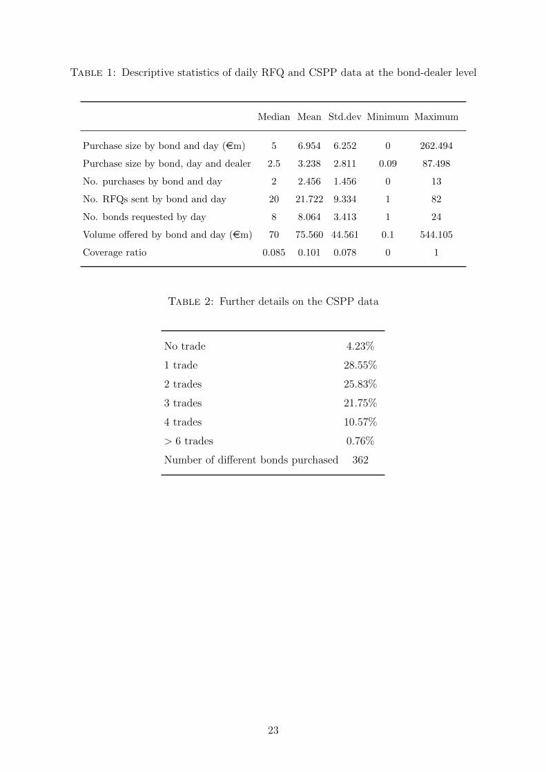
Table 1: Descriptive statistics of daily RFQ and CSPP data at the bond-dealer level

Median Mean Std.dev Minimum Maximum

Purchase size by bond and day (em) 5 6.954 6.252 0 262.494

Purchase size by bond, day and dealer 2.5 3.238 2.811 0.09 87.498

No. purchases by bond and day 2 2.456 1.456 0 13

No. RFQs sent by bond and day 20 21.722 9.334 1 82

No. bonds requested by day 8 8.064 3.413 1 24

Volume offered by bond and day (em) 70 75.560 44.561 0.1 544.105

Coverage ratio 0.085 0.101 0.078 0 1

Table 2: Further details on the CSPP data

No trade 4.23%

1 trade 28.55%

2 trades 25.83%

3 trades 21.75%

4 trades 10.57%

> 6 trades 0.76%

Number of different bonds purchased 362

23

Table 3: Liquidity measures

Liquidity measure description facet of liquidity meaning of the measure

Bid-ask spread difference between ask price and bid price tightness the lower the BAS (i.e. the lower the transaction

(BAS) (in bps) costs) the better are liquidity conditions

Roll effective bid-ask price tightness see bid-ask spread

Daily range absolute difference between high and low immediacy a wide range indicates that the market is less able

prices (in bps) for each day to absorb new orders (i.e. liquidity deteriorates)

Time to unwind The no. of days to exit a e5m position immediacy lower values indicate higher liquidity

Traded volume daily transactions (30 day avg trading depth high volume means high liquidity

volume) in em

Amihud absolute 1 day price return (in bps) depth higher values mean a high price impact and, thus,

divided by trading volume poor liquidity

Ticket size in em resilience higher values indicate higher liquidity

No. dealers No. of dealers quoting the bond over one day resilience higher values indicate higher liquidity

No. quotes No. of unique quotes received for an resilience higher values indicate higher liquidity

instrument over one day

24

Table 4: Mean values of the liquidity measures: bonds purchased by Bundesbank

Liquidity measure before after

10 March 2016 10 March 2016

bid-ask spread (in bps) 47.18 35.22

Roll (in bps) 10.78 6.79

Daily range (in bps) 79.61 59.44

Time to unwind (in days) 10.21 10.96

Traded volume (in em) 2.29 2.50

Amihud (in bps) 23.51 13.82

Ticket size (in em) 0.58 0.76

No. dealers 9.39 12.22

No. quotes 38.25 136.67

Source: Markit, Euroclear.

bps: basis points

25

Table 5: Mean values of the liquidity measures: German eligible bonds not purchased


10 March 2016 10 March 2016


Roll (in bps) 15.15 8.78







No. quotes 32.42 121.38


bps: basis points

Table 6: Mean values of the liquidity measures: eligible bonds not purchased


10 March 2016 10 March 2016


Roll (in bps) 12.75 7.22







No. quotes 33.29 135.88


bps: basis points

26

Table 7: Mean values of the liquidity measures: non-eligible investment grade bonds


10 March 2016 10 March 2016


Roll (in bps) 13.80 7.97







No. quotes 37.25 126.01


bps: basis points

Table 8: Mean values of the liquidity measures: non-eligible high yield bonds


10 March 2016 10 March 2016


Roll (in bps) 19.04 21.50







No. quotes 30.14 82.95


bps: basis points

27

Table 9: Flow effects using eligible but not purchased bonds as a control group

(1) (2) (3) (4) (5) (6) (7) (8) (9)

Amihud Bid-ask Time to unwind No. dealers No. quotes Ticket size Traded volume Range Roll

Volume purchased in em 0.0131 -0.0942∗∗∗ -0.0987 0.0286∗∗ -0.00438 0.00588∗∗ 0.0848∗∗ -0.134 -0.0170

(0.153) (0.0331) (0.0714) (0.0122) (0.284) (0.00294) (0.0390) (0.175) (0.0396)

No. RFQs sent 0.0859 0.0591∗∗ -0.0339 0.0210∗∗ -0.194 -0.00255 -0.0281 0.122 0.0294

(0.0966) (0.0250) (0.0462) (0.00904) (0.271) (0.00217) (0.0285) (0.137) (0.0254)

No. purchases -0.0962 -0.258∗∗ 0.503∗ 0.0175 -0.457 -0.00920 -0.0898 -0.749 -0.0608

(0.551) (0.104) (0.278) (0.0512) (1.193) (0.00851) (0.0913) (0.570) (0.105)

Volume offered in em -0.0205 -0.00873 -0.00524 0.00306 0.172∗∗∗ 0.00125∗ 0.0157 0.0138 0.00128

(0.0186) (0.00532) (0.0102) (0.00198) (0.0555) (0.000735) (0.0107) (0.0341) (0.00641)

N 3714 3727 3714 3724 3724 3714 3714 3681 3727

R2 0.460 0.905 0.456 0.797 0.727 0.498 0.469 0.541 0.651

adj. R2 0.309 0.878 0.303 0.740 0.650 0.357 0.320 0.412 0.554

Clustered standard errors in parentheses∗ p < 0.1, ∗∗ p < 0.05, ∗∗∗ p < 0.01

Notes: The Table reports estimation results from equation (1). Amihud, bid-ask spread, range and Roll are measured in bps, time to

unwind is in days, ticket size and traded volume in em. Standard errors are clustered by bond.

28

Table 10: Flow effects using ineligible IG as a control group

(1) (2) (3) (4) (5) (6) (7) (8) (9)


Volume purchased in em -0.180∗∗ -0.190∗∗∗ -0.125∗∗∗ 0.0561∗∗∗ 0.0862 0.0130∗∗∗ 0.142∗∗∗ -0.0681 0.0173

(0.0778) (0.0306) (0.0460) (0.0119) (0.262) (0.00317) (0.0318) (0.136) (0.0239)

N 153941 157811 153941 157664 157664 153941 153941 153024 157811

R2 0.297 0.794 0.310 0.730 0.652 0.171 0.140 0.449 0.401

adj. R2 0.290 0.792 0.303 0.727 0.648 0.163 0.132 0.444 0.395




29

Table 11: Flow effects using ineligible HY as a control group

(1) (2) (3) (4) (5) (6) (7) (8) (9)


Volume purchased in em -0.0727 -0.175∗∗ -0.101∗∗ 0.0569∗∗∗ -0.334 0.0109∗∗∗ 0.131∗∗∗ -0.181 0.00180

(0.0823) (0.0677) (0.0473) (0.0125) (0.274) (0.00311) (0.0329) (0.177) (0.0530)

N 71012 72716 71012 72661 72661 71012 71012 69595 72716

R2 0.234 0.720 0.563 0.665 0.627 0.448 0.363 0.571 0.361

adj. R2 0.219 0.714 0.554 0.658 0.620 0.438 0.351 0.562 0.349




30

Table 12: Flow effects for old bonds using eligible but not purchased bonds as a control group

(1) (2) (3) (4) (5) (6) (7) (8) (9)

Amihud Bid-ask ttu no dealer no quotes ticketsize tradevol range Roll

volume purchased in emn 0.119 0.0117 -0.197 0.0180 -0.664 0.00546 0.0125 -0.194 0.00479

(0.460) (0.0569) (0.247) (0.0241) (0.630) (0.00525) (0.0125) (0.241) (0.0407)

total rfq -0.0920 0.00327 -0.153 0.0262 -0.830∗ -0.00166 -0.00734 -0.191 0.0496∗

(0.270) (0.0379) (0.107) (0.0163) (0.491) (0.00354) (0.00847) (0.193) (0.0284)

no. of trades 0.114 -0.271 1.334∗∗ 0.0482 4.111∗∗ -0.0246 -0.0314 -0.214 -0.145

(1.287) (0.192) (0.665) (0.0840) (1.910) (0.0158) (0.0332) (0.934) (0.123)

volume offered in emn -0.0444 -0.00167 -0.0184 0.00285 0.140 0.00204∗ 0.00683∗∗∗ 0.0812 -0.00825

(0.0626) (0.00872) (0.0286) (0.00376) (0.136) (0.00121) (0.00234) (0.0837) (0.00916)

N 1176 1190 1176 1188 1188 1176 1176 1172 1190

R2 0.568 0.949 0.517 0.841 0.809 0.601 0.682 0.744 0.778

adj. R2 0.277 0.914 0.191 0.734 0.682 0.333 0.467 0.572 0.629

Standard errors in parentheses∗ p < 0.1, ∗∗ p < 0.05, ∗∗∗ p < 0.01



31

Table 13: Flow effects using eligible but not purchased bonds as a control group: heterogeneity across bonds and time

Move Term spread Business climate Age Size Residual maturity

Amihud 0.0134 0.228 0.00218 -0.0894** 0.000129 0.0517

(0.0111) (0.453) (0.0620) (0.0422) (0.000119) (0.0500)

Bid-ask spread -0.00528* 0.108 0.0255 0.0448*** -0.0000287 -0.0349***

(0.00270) (0.110) (0.0188) (0.0113) (0.0000456) (0.0124)

Time to unwind 0.0162*** -0.0703 -0.0580* -0.0679*** 0.000180** 0.0269

(0.00517) (0.247) (0.0330) (0.0236) (0.0000762) (0.0203)

No. dealers 0.00131 -0.178*** -0.0177*** -0.000472 -0.00000860 0.00628

(0.000925) (0.0482) (0.00660) (0.00378) (0.0000216) (0.00404)

No. quotes -0.0353* -0.358 0.108 -0.168 -0.000297 0.419***

(0.0209) (0.669) (0.158) (0.121) (0.000542) (0.116)

Ticket size 0.0000450 0.00167 -0.000410 -0.000401 0.00000268 0.000184

(0.000249) (0.00955) (0.00151) (0.00139) (0.00000573) (0.00146)

Traded volume 0.00212 0.0668 -0.0242 -0.0471*** 0.0000862 0.0244*

(0.00292) (0.0852) (0.0167) (0.0131) (0.0000679) (0.0129)

Range -0.0152 -0.0108 0.0937 -0.0171 0.000117 0.0536

(0.0165) (0.495) (0.0831) (0.0589) (0.000335) (0.0598)

Roll -0.00151 0.201* 0.0237 0.000531 0.0000853 -0.0120

(0.00255) (0.108) (0.0168) (0.00993) (0.0000724) (0.0110)

Notes : The Table reports the estimates of the interaction coefficient φ from equation (2). Amihud, bid-ask spread, range and Roll are

measured in bps, time to unwind is in days, ticket size and traded volume in em. Standard errors are clustered by bond.

32

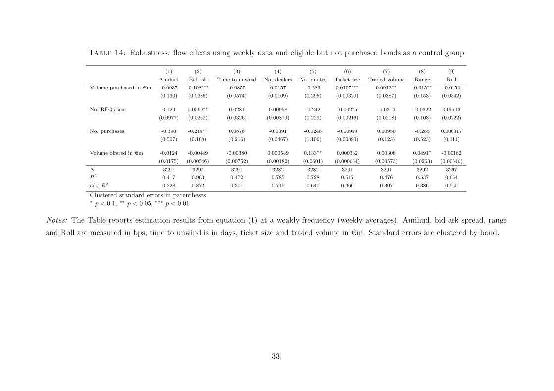
Table 14: Robustness: flow effects using weekly data and eligible but not purchased bonds as a control group

(1) (2) (3) (4) (5) (6) (7) (8) (9)


Volume purchased in em -0.0937 -0.108∗∗∗ -0.0855 0.0157 -0.283 0.0107∗∗∗ 0.0912∗∗ -0.315∗∗ -0.0152

(0.130) (0.0336) (0.0574) (0.0109) (0.295) (0.00320) (0.0387) (0.153) (0.0342)

No. RFQs sent 0.129 0.0560∗∗ 0.0281 0.00958 -0.242 -0.00275 -0.0314 -0.0322 0.00713

(0.0977) (0.0262) (0.0326) (0.00879) (0.229) (0.00216) (0.0218) (0.103) (0.0222)

No. purchases -0.390 -0.215∗∗ 0.0876 -0.0391 -0.0248 -0.00959 0.00950 -0.285 0.000317

(0.507) (0.108) (0.216) (0.0467) (1.106) (0.00890) (0.123) (0.523) (0.111)

Volume offered in em -0.0124 -0.00449 -0.00380 0.000549 0.133∗∗ 0.000332 0.00308 0.0491∗ -0.00162

(0.0175) (0.00546) (0.00752) (0.00182) (0.0601) (0.000634) (0.00573) (0.0263) (0.00546)

N 3291 3297 3291 3282 3282 3291 3291 3292 3297

R2 0.417 0.903 0.472 0.785 0.728 0.517 0.476 0.537 0.664

adj. R2 0.228 0.872 0.301 0.715 0.640 0.360 0.307 0.386 0.555


Notes: The Table reports estimation results from equation (1) at a weakly frequency (weekly averages). Amihud, bid-ask spread, range

and Roll are measured in bps, time to unwind is in days, ticket size and traded volume in em. Standard errors are clustered by bond.

33

Table 15: Stock effects using eligible but not purchased bonds as a control group

(1) (2) (3) (4) (5) (6) (7) (8) (9)


CSPP total purchases (in b euro) 78.84 33.13∗ 0.839 -11.67∗∗∗ -76.72∗∗ 0.799 -0.445 58.20∗ 26.98∗∗

(54.63) (19.22) (16.94) (3.668) (35.17) (0.800) (3.393) (34.48) (12.01)

Amount issued (in b euro) 0.850 1.684 -2.761 -1.607∗∗∗ -22.19∗∗∗ 0.197 -2.009∗∗∗ -7.943 -0.292

(6.501) (3.494) (3.108) (0.566) (5.726) (0.157) (0.653) (8.964) (2.512)

Age -2.408∗∗ 0.757∗ -0.781∗ 0.110 0.634 0.0430 0.471∗∗∗ 2.544∗∗ 1.103∗∗

(1.094) (0.429) (0.422) (0.0793) (0.851) (0.0284) (0.100) (1.152) (0.500)

Rating 0.373 0.651 -0.809 -0.428∗∗ -3.632∗∗ -0.0480 0.237∗∗ 1.619 1.299

(1.961) (0.889) (1.061) (0.176) (1.599) (0.0659) (0.118) (2.729) (0.795)

Residual maturity -1.424 1.639∗ 1.830 0.399∗∗ 1.318 -0.203∗∗∗ -0.0545 4.144 -0.243

(2.036) (0.968) (1.236) (0.201) (1.702) (0.0677) (0.202) (2.653) (0.986)

Yield spread to matched Bund (in %) 7.415∗ -4.981 2.952 -0.425 2.385 0.0497 -1.047∗∗ -11.02 -1.999

(3.937) (3.135) (1.923) (0.435) (3.819) (0.120) (0.442) (8.604) (3.363)

Amount outst. matched Bund (in b euro) 0.233 -0.335 0.792 0.198∗ 1.828∗∗ -0.0537∗ 0.0785 1.539 0.175

(1.025) (0.579) (0.635) (0.109) (0.896) (0.0272) (0.0920) (1.343) (0.518)

∆ Rating 1.476 1.595 -1.000 -0.264 -3.140 -0.0844 0.366∗ 9.347 2.539

(3.301) (2.124) (1.671) (0.369) (3.051) (0.0938) (0.221) (6.930) (1.615)

∆ Amount outst. matched Bund (in b euro) 0.000326 -0.00150∗∗ 0.000116 0.000157 0.000354 -0.0000568 0.0000435 0.00147 -0.00102

(0.00116) (0.000757) (0.000690) (0.000157) (0.00134) (0.0000344) (0.000172) (0.00191) (0.000703)

PSPP total purchases (in b euro) -1.283 0.692 -3.594 -0.573 -3.098 0.324∗∗∗ 0.264 -5.753 -0.742

(3.870) (1.882) (2.289) (0.419) (3.500) (0.112) (0.320) (4.828) (1.602)

Constant -5.305 -29.05∗∗ -9.756 -6.719∗∗∗ -25.38 2.227∗∗ -1.749 -79.60∗∗ -23.91∗

(23.85) (13.97) (17.41) (2.510) (22.14) (0.920) (2.415) (37.18) (13.52)

Industry indicators Yes Yes Yes Yes Yes Yes Yes Yes Yes

N 206 210 206 210 210 206 206 199 210

R2 0.174 0.255 0.084 0.357 0.421 0.147 0.335 0.123 0.275

adj. R2 0.095 0.185 -0.004 0.296 0.366 0.065 0.271 0.035 0.206

p-values in parentheses∗ p < 0.1, ∗∗ p < 0.05, ∗∗∗ p < 0.01


unwind is in days, ticket size and traded volume in em. Standard errors are robust to heteroscedasticity.

34

Table 16: Stock effects using ineligible IG bonds as a control group

(1) (2) (3) (4) (5) (6) (7) (8) (9)


CSPP total purchases (in b euro) 52.47 28.46 18.23 0.585 -23.17 0.157 2.779 86.47∗∗ 32.86∗∗

(46.34) (21.25) (22.74) (5.287) (55.13) (1.291) (9.430) (41.57) (13.06)

Amount issued (in b euro) 23.77 6.048 -5.582 -3.255 -11.57 0.117 2.487 -12.75 -8.357

(15.29) (9.698) (10.73) (2.073) (22.34) (0.779) (5.633) (27.81) (6.550)

Age -0.154 0.337 -1.450 0.185 5.806∗∗ 0.0509 1.175 -2.877 1.289∗∗

(2.131) (0.973) (1.170) (0.277) (2.730) (0.0735) (0.759) (2.855) (0.624)

Rating 6.417∗ 4.112∗∗ 0.462 0.854∗∗ 5.253∗ -0.0933 -1.809 1.812 5.007∗∗∗

(3.723) (1.830) (2.259) (0.323) (3.125) (0.159) (1.759) (7.941) (1.111)

Residual maturity 5.272 2.190 4.925 0.118 6.235∗ -0.419∗ -1.285 8.315 -0.224

(5.996) (1.761) (4.590) (0.358) (3.251) (0.214) (2.112) (5.919) (1.424)

Yield spread to matched Bund (in %) -9.044∗∗ -9.630∗∗∗ -1.258 -2.005∗∗∗ -16.90∗∗∗ 0.132 0.983 -19.35∗∗∗ -9.406∗∗∗

(4.043) (1.786) (2.690) (0.319) (2.840) (0.174) (1.718) (5.002) (1.612)

Amount outst. matched Bund (in b euro) 2.144 -0.425 1.586 0.154 2.092 -0.150 -0.679 2.011 0.0801

(2.668) (1.155) (1.983) (0.223) (1.706) (0.100) (1.182) (3.369) (0.878)

∆ Rating -2.407 -0.0940 -0.636 0.831 -0.847 -0.0957 -1.716 -16.37 4.395

(3.935) (3.340) (2.092) (0.701) (5.733) (0.236) (2.504) (18.05) (2.776)

∆ Amount outst. matched Bund (in b euro) 0.00212 -0.00155 0.000744 0.0000683 0.000508 -0.000148 -0.000578 -0.00162 -0.000633

(0.00254) (0.00160) (0.00192) (0.000329) (0.00220) (0.000121) (0.00134) (0.00392) (0.00119)

PSPP total purchases (in b euro) -7.909 2.905 -5.772 0.00311 -5.575 0.539 2.621 -5.006 0.474

(9.409) (3.721) (7.367) (0.734) (5.451) (0.376) (4.196) (10.82) (2.901)

Constant -114.3 -55.76∗ -42.28 -11.82∗∗ -108.0∗ 4.947∗ 18.90 -86.06 -35.38∗

(82.04) (28.38) (53.94) (5.429) (59.27) (2.729) (21.97) (86.70) (18.51)


N 67 67 67 67 67 67 67 66 67

R2 0.296 0.477 0.192 0.544 0.555 0.330 0.183 0.257 0.632

adj. R2 0.052 0.296 -0.088 0.385 0.400 0.098 -0.101 -0.005 0.504




35

Table 17: Stock effects using ineligible HY bonds as a control group

(1) (2) (3) (4) (5) (6) (7) (8) (9)


CSPP total purchases (in b euro) 186.1∗∗ 17.62 71.47 7.021 -31.33 -2.376 -7.771 64.88 123.8∗

(79.41) (46.22) (52.14) (6.098) (47.45) (2.264) (4.605) (83.90) (71.16)

Amount issued (in b euro) -37.33 34.45 -43.25 -5.421∗ -17.42 1.987 -2.167 83.73∗ 6.203

(38.08) (22.65) (30.05) (2.964) (17.52) (1.365) (2.240) (44.13) (29.94)

Age 0.321 4.017∗∗∗ -1.412 0.0190 0.330 0.121∗ 0.514∗∗∗ -0.984 2.209

(2.100) (1.436) (1.196) (0.201) (1.044) (0.0623) (0.127) (2.420) (2.239)

Rating 2.379 -0.482 -1.104 0.0834 -1.462 -0.106 -0.674∗∗∗ 6.463 11.22∗∗∗

(3.179) (2.296) (2.095) (0.367) (1.592) (0.119) (0.243) (4.380) (2.994)

Residual maturity 2.385 2.147 2.599 -0.257 -0.887 -0.0930 0.111 5.148∗∗ 2.967∗

(2.918) (1.289) (2.453) (0.168) (0.938) (0.115) (0.149) (2.274) (1.673)

Yield spread to matched Bund (in %) -0.0325 1.896 1.363 -0.352 2.594 0.0746 0.593∗∗ -11.70∗∗ -2.388

(4.000) (3.063) (2.875) (0.445) (1.854) (0.151) (0.262) (5.225) (5.191)

Amount outst. matched Bund (in b euro) 1.364 -0.702 0.409 -0.0613 0.151 0.0441 0.418∗∗∗ -1.451 -0.982

(1.716) (1.323) (1.205) (0.186) (0.910) (0.0588) (0.121) (2.092) (1.689)

∆ Rating 11.12∗ 10.79∗ 1.766 -1.530∗∗ -19.93∗∗∗ -0.0653 0.737∗ 13.22 70.66∗∗∗

(5.691) (6.327) (4.111) (0.747) (3.959) (0.209) (0.375) (8.569) (10.58)

∆ Amount outst. matched Bund (in b euro) -0.00525 -0.00166 -0.00446 0.0000939 0.000743 0.000240∗ 0.000403∗∗ -0.000333 -0.00127

(0.00372) (0.00130) (0.00289) (0.000272) (0.00124) (0.000132) (0.000153) (0.00318) (0.00217)

PSPP total purchases (in b euro) -2.482 6.251 -1.155 0.149 -3.353 -0.0821 -1.472∗∗∗ 4.303 1.397

(6.611) (4.608) (5.145) (0.530) (3.169) (0.253) (0.445) (6.543) (5.507)

Constant -51.13 -60.89∗∗∗ 11.42 -3.437 5.540 -0.310 0.491 -135.1∗∗∗ -129.2∗∗∗

(38.46) (21.39) (17.75) (2.777) (22.29) (1.038) (2.643) (41.72) (42.84)


N 52 52 52 52 52 52 52 52 52

R2 0.385 0.732 0.243 0.650 0.739 0.318 0.617 0.658 0.869

adj. R2 0.078 0.599 -0.135 0.475 0.609 -0.024 0.425 0.487 0.803




36

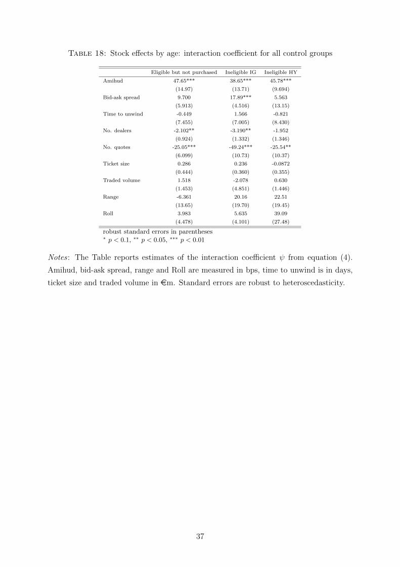
Table 18: Stock effects by age: interaction coefficient for all control groups

Eligible but not purchased Ineligible IG Ineligible HY

Amihud 47.65*** 38.65*** 45.78***

(14.97) (13.71) (9.694)

Bid-ask spread 9.700 17.89*** 5.563

(5.913) (4.516) (13.15)

Time to unwind -0.449 1.566 -0.821

(7.455) (7.005) (8.430)

No. dealers -2.102** -3.190** -1.952

(0.924) (1.332) (1.346)

No. quotes -25.05*** -49.24*** -25.54**

(6.099) (10.73) (10.37)

Ticket size 0.286 0.236 -0.0872

(0.444) (0.360) (0.355)

Traded volume 1.518 -2.078 0.630

(1.453) (4.851) (1.446)

Range -6.361 20.16 22.51

(13.65) (19.70) (19.45)

Roll 3.983 5.635 39.09

(4.478) (4.101) (27.48)

robust standard errors in parentheses∗ p < 0.1, ∗∗ p < 0.05, ∗∗∗ p < 0.01

Notes : The Table reports estimates of the interaction coefficient ψ from equation (4).

Amihud, bid-ask spread, range and Roll are measured in bps, time to unwind is in days,

ticket size and traded volume in em. Standard errors are robust to heteroscedasticity.

37

Table 19: Stock effects by amount issued: interaction coefficient for all control groups


Amihud -74.70 -42.97 -180.8

(152.5) (116.0) (194.8)

Bid-ask spread 12.24 -30.14 -77.82

(58.72) (72.32) (134.7)

Time to unwind -80.68 -138.1 -212.8

(91.34) (117.5) (185.8)

No. dealers 31.93*** 13.56 24.70

(9.651) (15.72) (15.02)

No. quotes 246.5*** 165.3 174.6

(81.99) (153.6) (130.6)

Ticket size -0.841 2.657 7.593

(3.514) (5.569) (7.637)

Traded volume -27.86*** -56.88 -26.14

(10.56) (41.13) (15.88)

Range 236.8** 94.14 -184.3

(117.4) (184.1) (285.7)

Roll -32.47 -32.32 -182.9

(50.90) (52.02) (254.9)





38

Table 20: Stock effects by residual maturity: interaction coefficient for all control

groups


Amihud 12.73 -10.52 30.15

(22.67) (25.78) (28.38)

Bid-ask spread 4.270 0.300 19.10

(8.148) (14.43) (18.57)

Time to unwind 18.76 17.62 35.50

(12.46) (17.67) (26.20)

No. dealers -2.283 2.685 -2.245

(1.720) (2.874) (2.179)

No. quotes 0.537 3.419 1.688

(16.94) (27.76) (16.85)

Ticket size -0.460 -0.606 -1.523

(0.575) (1.029) (1.327)

Traded volume 0.865 4.531 1.492

(1.920) (8.342) (2.042)

Range 14.74 -1.309 0.0974

(23.49) (33.61) (38.92)

Roll 2.077 -0.493 -31.43

(7.504) (10.12) (23.82)





39

Table 21: Robustness: stock effects for all control groups: using a window of 2 weeks


Amihud 47.65*** 38.65*** 45.78***

(14.97) (13.71) (9.694)

Bid-ask spread 9.700 17.89*** 5.563

(5.913) (4.516) (13.15)

Time to unwind -0.449 1.566 -0.821

(7.455) (7.005) (8.430)

No. dealers -2.102** -3.190** -1.952

(0.924) (1.332) (1.346)

No. quotes -25.05*** -49.24*** -25.54**

(6.099) (10.73) (10.37)

Ticket size 0.286 0.236 -0.0872

(0.444) (0.360) (0.355)

Traded volume 1.518 -2.078 0.630

(1.453) (4.851) (1.446)

Range -6.361 20.16 22.51

(13.65) (19.70) (19.45)

Roll 3.983 5.635 39.09

(4.478) (4.101) (27.48)

robust standard errors in parentheses

∗ p < 0.1, ∗∗ p < 0.05, ∗∗∗ p < 0.01

Notes : The Table reports estimates of β from equation (3). Amihud, bid-ask spread,

range and Roll are measured in bps, time to unwind is in days, ticket size and traded

volume in em. Standard errors are robust to heteroscedasticity.

40

Table 22: Robustness: stock effects for all control groups: using a window of 4 weeks


Amihud 55.37 41.36 7.834

(37.59) (37.24) (64.42)

Bid-ask spread 0.0544 25.23* 53.54*

(10.58) (14.68) (29.02)

Time to unwind 31.63 41.55 66.15

(25.42) (25.56) (56.30)

No. dealers -11.40*** 0.937 -3.470

(3.426) (3.171) (6.230)

No. quotes -189.1** -115.7 3.045

(88.16) (80.43) (54.21)

Ticket size -2.030** -0.488 -1.370

(0.889) (1.017) (1.257)

Traded volume -5.143 13.73 -10.80**

(3.189) (12.79) (4.889)

Range 9.089 71.42 144.9*

(43.84) (49.22) (73.89)

Roll 24.89** 27.48*** 63.65

(10.69) (9.251) (79.42)

robust standard errors in parentheses

∗ p < 0.1, ∗∗ p < 0.05, ∗∗∗ p < 0.01

Notes : The Table reports estimates of β from equation (3). Amihud, bid-ask spread,

range and Roll are measured in bps, time to unwind is in days, ticket size and traded

volume in em. Standard errors are robust to heteroscedasticity.

41

Figure 1: Bundesbank CSPP Purchases by month and sector

050

010

0015

0020

0025

00A

vera

ge m

onth

ly p

urch

ase

volu

me

2016m7 2017m1 2017m7 2018m1 2018m7 2019m1Date

Utilities TechnologyIndustrial GovernmentFinancial EnergyConsumer, Non-Cyclical Consumer, CyclicalCommunications Basic Materials

42

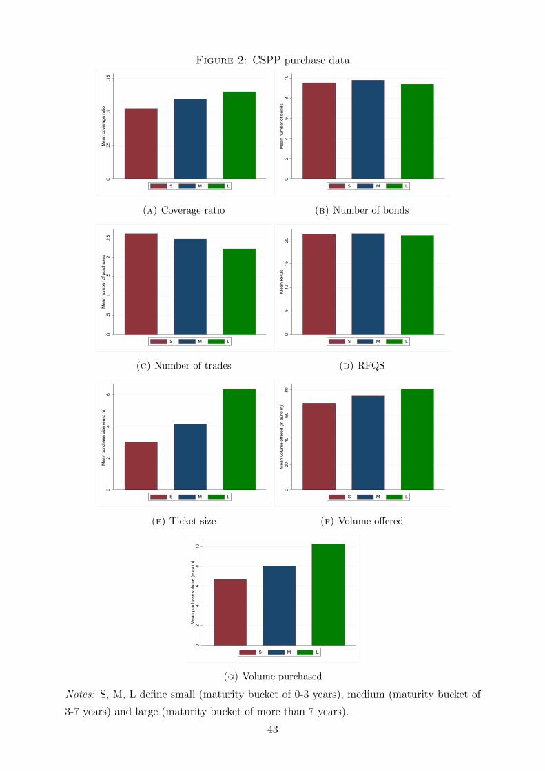
Figure 2: CSPP purchase data

0.0

5.1

.15

Mea

n co

vera

ge ra

tio

S M L

(a) Coverage ratio

02

46

810

Mea

n nu

mbe

r of b

onds

S M L

(b) Number of bonds

0.5

11.

52

2.5

Mea

n nu

mbe

r of p

urch

ases

S M L

(c) Number of trades

05

1015

20M

ean

RFQ

s

S M L

(d) RFQS

02

46

Mea

n pu

rcha

se s

ize

(eur

o m

)

S M L

(e) Ticket size

020

4060

80M

ean

volu

me

offe

red

(in e

uro

m)

S M L

(f) Volume offered

02

46

810

Mea

n pu

rcha

se v

olum

e (e

uro

m)

S M L

(g) Volume purchased

Notes: S, M, L define small (maturity bucket of 0-3 years), medium (maturity bucket of

3-7 years) and large (maturity bucket of more than 7 years).

43

Figure 3: Evolution of liquidity measures (facet of tightness)

020

4060

8010

0in

bp

2015m1 2016m1 2017m1 2018m1 2019m1date

purchased eligible, not purchasednon-eligible IG non-eligible HY

(a) Bid-ask spread

010

2030

40in

bp

2015m1 2016m1 2017m1 2018m1 2019m1date


(b) Roll

Notes: The vertical red lines point to the announcement of the CSPP on 10 March 2016,

the start of the CSPP on 8 June 2018, and to the end of the net purchases on 31 December

2018, respectively.

Figure 4: Evolution of liquidity measures (facet of immediacy)

050

100

150

200

in b

p

2015m1 2016m1 2017m1 2018m1 2019m1date


(a) Daily range

05

1015

in d

ays

2015m1 2016m1 2017m1 2018m1 2019m1date


(b) Time to unwind



2018, respectively.

44

Figure 5: Evolution of liquidity measures (facet of depth)

01

23

45

6in

mn

€

2015m1 2016m1 2017m1 2018m1 2019m1date


(a) Traded volume

48

1216

20in

bp

2015m1 2016m1 2017m1 2018m1 2019m1date


(b) Amihud



2018, respectively.

45

Figure 6: Evolution of liquidity measures (facet of resilience)

.2.6

1in

mm

€

2015m1 2016m1 2017m1 2018m1 2019m1date


(a) Ticket size

59

1317

2015m1 2016m1 2017m1 2018m1 2019m1date


(b) No. dealers

050

100

150

200

250

300

2015m1 2016m1 2017m1 2018m1 2019m1date


(c) No. quotes



2018, respectively.

46

Figure 7: Marginal effects for the flow regressions for selected liquidity indicators,

bond characteristics and economic time series-.2

0.2

.4.6

.8M

argi

nal e

ffect

0 2 4 6 8 10 12 14 16Age (in years)

(a) Marginal effect of CSPP purchases on

bid-ask spreads depending on bond age

-.50

.51

Mar

gina

l effe

ct

42 50 58 66 74 82 90 98MOVE index

(b) Marginal effect of CSPP purchases on

time to unwind depending on the MOVE

index

-.10

.1.2

Mar

gina

l effe

ct

.3 .5 .7 .9 1.1 1.3Term spread (in pp)

(c) Marginal effect of CSPP purchases on

no. dealers depending on the term spread

-.05

0.0

5.1

.15

Mar

gina

l effe

ct

98 99 100 101 102 103 104 105Business climate

(d) Marginal effect of CSPP purchases on

no. dealers depending on the business

climate

Notes : The Figures use eligible but not purchased bonds as a control group. Marginal

effects are shown together with 95% confidence intervals.

47

Figure 8: Marginal effects for the stock regressions for selected liquidity indicators and

bond characteristics-2

000

200

400

600

800

Mar

gina

l effe

ct

0 2 4 6 8 10 12Age (in years)

(a) Marginal effect of CSPP purchases on

the Amihud measure depending on age

-400

-300

-200

-100

0M

argi

nal e

ffect

0 2 4 6 8 10 12Age (in years)

(b) Marginal effect of CSPP purchases on

number of quotes depending on age

-40

-20

020

40M

argi

nal e

ffect

0 .5 1 1.5 2Size (in bn euros)

(c) Marginal effect of CSPP purchases on

trading volume depending on size

-200

020

040

060

0M

argi

nal e

ffect

0 .5 1 1.5 2Size (in bn euros)

(d) Marginal effect of CSPP purchases on

the range depending on size

Notes : The Figures use eligible but not purchased bonds as a control group. Marginal

effects are shown together with 95% confidence intervals.

48

liquidity in the german corporate bond market: has the

Documents