Liquid-Solid Mass Transfer in Conventional and Inverse Fluidized

Beds

by

Victer Veldman

Dissertation presented in partial fulfilment of the requirements

for the degree of

Master of Engineering in Chemical Engineering at the University of Pretoria

Faculty of Engineering, the Built Environment and Information Technology

Department of Chemical Engineering

University of Pretoria

Supervisor: Prof. W. Nicol

November 2012

i

Synopsis

Liquid-solid mass transfer was experimentally determined on a novel reactor,

with external recycling. Liquid-solid experiments were performed in both up-

flow and down-flow mode depending on the particle density. In addition, three-

phase experiments were performed in concurrent up-flow mode. The

dissolution of benzoic acid method was adapted and used in order to quantify

the liquid-solid mass transfer rate.

It was found that the direction of liquid flow had no influence on liquid-solid

mass transfer for two-phase fluidized beds. It was, however, found that the

density difference between the solid particle and liquid (Δρ) had a significant

influence on the liquid-solid mass transfer. For higher Δρ, higher mass

transfer coefficients were achieved. The liquid-solid mass transfer coefficient

increased until minimum fluidization was reached, after which the increase in

mass transfer was less severe with a further increase in liquid velocity.

The correlation proposed by Kawase and Moo-Young (1987) effectively fits

the experimental data from the minimum fluidization velocity (umf) until the

onset of turbulent velocity (uc). This correlation exhibits an absolute average

relative error (AARE) of 18% when the data points for all four particles are

compared with the correlation. A new correlation is proposed with the

inclusion of the dimensionless group, the Archimedes number. The correlation

proposed achieved an AARE of only 8%, and can be seen in the equation

below.

!ℎ = 0.05!"!.!"!"!.!!!"!.!"

A comparison between fluidized bed performance and packed bed

performance showed that the density difference determines the superior

mode of liquid-solid mass transfer. When Δρ is high, as for the alumina

particles Δρ = 1 300 kg/m3, the fluidized bed outperforms the packed bed.

When the density difference becomes smaller, Δρ = 580 kg/m3, the fluidized

ii

bed only slightly outperforms the packed bed setup, while for a very small

density difference (Δρ = -145 kg/m3) the packed bed substantially outperforms

the fluidized bed. This trend is irrespective of the direction of fluidization.

When Δρ is negative it indicates inverse fluidization.

With the introduction of gas to the system, higher liquid-solid mass transfer

coefficients were obtained at the same superficial liquid velocity. Furthermore,

no significant transitions were seen between the minimum fluidization and the

onset of turbulence flow regimes, as seen with two-phase fluidization. This

contributed to the gradual fluidization that was seen with three-phase

fluidization and not instantaneous fluidization, as with liquid-solid fluidized

beds.

Keywords: Liquid-solid mass transfer, inverse fluidization, conventional

fluidization

iii

Table of Contents

Synopsis ................................................................................. i  

List of Figures ......................................................................... v  

List of Tables ......................................................................... vii  

Nomenclature ....................................................................... viii  

1.   Introduction .................................................................... 1  

2.   Transport Parameters Prediction ..................................... 3  2.1 Liquid-solid conventional fluidized bed hydrodynamics .. . . . . . . . 3  

1.1.1   Minimum fluidization velocity (MFV) ......................................................... 4  1.1.2   Void fraction ............................................................................................. 5  

1.2   Liquid-solid-gas conventional fluidization hydrodynamics .. . 6  1.2.1   Minimum fluidization velocity (MFV) ......................................................... 6  1.2.2   Gas hold-up .............................................................................................. 7  1.2.3   Bubble properties ..................................................................................... 8  

1.3   Inverse fluidization hydrodynamics .. . . . . . . . . . . . . . . . . . . . . . . . . . . . . . . . . . 10  1.3.1   Minimum fluidization velocity .................................................................. 10  1.3.2   Void fraction ........................................................................................... 12  1.3.3   Liquid mixing (dispersion) ...................................................................... 13  

1.4   Liquid-solid mass transfer in two- and three-phase fluidized

beds 15  1.4.1   Literature correlations ............................................................................ 16  

3.   Experimental .................................................................. 19  3.1 Apparatus .. . . . . . . . . . . . . . . . . . . . . . . . . . . . . . . . . . . . . . . . . . . . . . . . . . . . . . . . . . . . . . . . . . . . . . . . . . . 19  

3.1.1 Reactor setup ............................................................................................ 19  3.2   Particles .. . . . . . . . . . . . . . . . . . . . . . . . . . . . . . . . . . . . . . . . . . . . . . . . . . . . . . . . . . . . . . . . . . . . . . . . . . . 25  

3.2.1   Types ..................................................................................................... 25  3.2.2   Particle preparation ................................................................................ 26  

3.3   Data interpretation .. . . . . . . . . . . . . . . . . . . . . . . . . . . . . . . . . . . . . . . . . . . . . . . . . . . . . . . . . . . 27  

4.   Results and discussions ................................................ 32  4.1   Repeatability . . . . . . . . . . . . . . . . . . . . . . . . . . . . . . . . . . . . . . . . . . . . . . . . . . . . . . . . . . . . . . . . . . . . . 32  

4.1.1   Influence of reactor length ...................................................................... 34  4.2   Two-phase liquid-solid mass transfer . . . . . . . . . . . . . . . . . . . . . . . . . . . . . . . . 35  

4.2.1   Fluidized bed .......................................................................................... 35  

iv

4.2.2   Packed bed ............................................................................................ 43  4.3   Three phase fluidization .. . . . . . . . . . . . . . . . . . . . . . . . . . . . . . . . . . . . . . . . . . . . . . . . . . . 46  

5.   Conclusions ................................................................... 51  

6.   References ..................................................................... 53  

7.   Appendices .................................................................... 58  7.1   Appendix A: Analytical calibrations .. . . . . . . . . . . . . . . . . . . . . . . . . . . . . . . . . . 58  7.2   Appendix B: Liquid-solid mass transfer plots .. . . . . . . . . . . . . . . . . . . 60  7.3   Appendix C: Expanded drawing of fluidized bed reactor .. . . 63  

v

List of Figures

Figure 2.1: Various contacting regimes in liquid fluidization (Kunii &

Levenspiel, 1999: 2) ................................................................................. 3  

Figure 2.2: The measured input and output RTD along with the deconvoluted

system RTD for a set of parameters ....................................................... 14  

Figure 2.3: Trends observed by Arters and Fan (1990), which show an

increase in mass transfer as gas velocity is increased ........................... 16  

Figure 3.1: A schematic flow diagram of the reactor setup used in all

experiments ............................................................................................ 20  

Figure 3.2: Representation of the fluidized bed reactor used in all

experiments ............................................................................................ 21  

Figure 3.3: Photos of the reactor a) assembled and b) dissembled (with two

different gas distributor designs) ............................................................. 22  

Figure 3.4: Liquid distributer design: a) top view b) side view ...................... 23  

Figure 3.5: a) Poraver particles ul = 0 m/s b) Poraver being fluidized in liquid-

down flow mode ul = 0.039 m/s c) alumina particles ul = 0 m/s d) alumina

being fluidized in liquid up-flow mode ul = 0.039 m/s .............................. 24  

Figure 3.6: Drawing of the bottom half of the inverse fluidized bed, where the

yellow part is the liquid distributor and the bronze part isthe gas

distributor. (a) and (b) represent the two different designs ..................... 24  

Figure 3.7: Particle density of Poraver particles measured with different

submersion times in water ...................................................................... 26  

Figure 3.8: Concentration of benzoic acid in a stagnant beaker setup against

time for coated polypropylene particles .................................................. 29  

Figure 3.9: Comparison between a true step prediction and an adapted

smooth prediction for the fluidization of polypropylene at a liquid velocity

of 10.5 mm/s ........................................................................................... 31  

Figure 4.1: a) Two identical runs done in a packed bed with polypropylene

particles (ul = 17 mm/s). b)Two identical runs done in a packed bed with

polypropylene particles(ul = 39 mm/s) .................................................... 33  

Figure 4.2: Two identical runs at ul = 30 mm/s and two at ul = 39 mm/s done

in a fluidized bed with Poraver particles ................................................. 33  

vi

Figure 4.3: Fluidized runs with polypropylene at a superficial liquid velocity of

26 mm/s .................................................................................................. 34  

Figure 4.4:Dissolution runs done with polypropylene at different superficial

liquid velocities ........................................................................................ 35  

Figure 4.5: Liquid-solid mass transfer as a function of superficial liquid

velocity for fluidization runs ..................................................................... 36  

Figure 4.6: Experimental results found with indication of critical liquid

superficial velocities ................................................................................ 38  

Figure 4.7: Comparison between experimental data and the correlation

proposed by Kawase & Moo-Young (1987). The circled data points fall in

the umf – uc window ................................................................................. 40  

Figure 4.8: Comparison between the new correlated model (Equation 4.3)

and the experimental results ................................................................... 42  

Figure 4.9: Thoenes and Kramers (1958) model compared to data obtained

in the packed bed setup for POM and Poraver ....................................... 44  

Figure 4.10: Comparison between packed bed performance and fluidized bed

performance for different Re and Ar values ............................................ 45  

Figure 4.11: Data obtained for liquid-solid mass transfer in two- and three-

phase fluidization (superficial gas velocity of 0.33 cm/s) for alumina

particles. umf and uc values are for the two-phase system ...................... 47  

Figure 4.12: Data for two- and three-phase systems with alumina particles

along with model predictions from Kawase and Moo-Young (1987). umf

and uc values are for the two-phase system ........................................... 49  

Figure 4.13: Data for two- and three-phase systems with POM particles along

with model predictions by Kawase and Moo-Young (1987). umf and uc

values are for the two-phase system ...................................................... 50  

vii

List of Tables Table 2.1: Models for MFV in three-phase inverse fluidization ..................... 12  

Table 2.2: Literature correlations for α, β and γ for use in Equation (2.32) ... 18  

Table 3.1: List off all equipment used in experiments and shown in Figure 3.1

................................................................................................................ 20  

Table 3.2: Different particles used in this study ............................................. 25  

Table 3.3: Different particles coated with the amount of benzoic acid (BA)

added ...................................................................................................... 27  

Table 3.4: Fit criteria for the four particle types. Partial coverage occurs at

CPC .......................................................................................................... 30  

Table 4.1: The AARE of liquid-solid mass transfer coefficient for repeat runs

................................................................................................................ 32  

Table 4.2: Density differences and Reynolds numbers at umf and uc ............ 39  

viii

Nomenclature Symbol Description Units

as Total external area of coated particles m2

Acol Area of column m2

Ar Archimedes number -

CAb Concentration of benzoic acid in water kg/m3

Csat Saturation concentration of benzoic acid in water at

30 oC kg/m3

Cv Volumetric solid concentration v/v

CPC Concentration at which partial coverage occurs g/l

Cmax Maximum concentration possible inside reactor g/l

d* Dimensionless particle diameter -

do Diameter of orifice in sparger mm

dp Particle diameter m

DC Column diameter m

Dl Axial dispersion coefficient m2/s

e Energy dissipated per unit mass of liquid m2/s2

FB Bubble frequency -

Hbed Bed height m

Kd Distributor coefficient -

ks Liquid-solid mass transfer coefficient m/s

Lv Bubble size m

No Number of orifices in sparger -

PT Total pressure kg/ms2

PS Vapour pressure of liquid kg/ms2

Pe Peclet number -

Rec Reynolds number at uc -

Relmfo Reynolds number at minimum fluidization with no gas flow

-

Remf Reynolds number at minimum fluidization -

Ret∞ Reynolds number of one particle in infinite medium -

ix

Sc Schmidt number -

Sh Sherwood number -

ShFB Sherwood number for fluidized bed -

ShPB Sherwood number for packed bed -

Shexp Experimentally determined Sherwood number -

u* Dimensionless terminal velocity -

uc Onset of turbulent regime liquid velocity m/s

umf Minimum fluidization velocity m/s

ug Superficial gas velocity m/s

ul Liquid superficial velocity m/s

ut Terminal velocity m/s

UB Bubble rise velocity m/s

vvm Volume of gas fed to reactor per volume of reactor

per minute ml/ml.min

V Volume of reactor m3

Vsamp Volume of samples taken m3

Greek Symbols

α Equation constant in Equation (2.32) -

β Equation constant in Equation (2.32) -

γ Equation constant in Equation (2.32) -

ε Void fraction -

εg Gas hold-up -

µl Liquid viscosity Pa.s

ρl Liquid density kg/m3

ρg Gas density kg/m3

Δρ Density difference between liquid and solid phases kg/m3

Δz Distance between measuring points mm

Φ Sphericity -

 ν   Kinematic viscosity m2/s

1

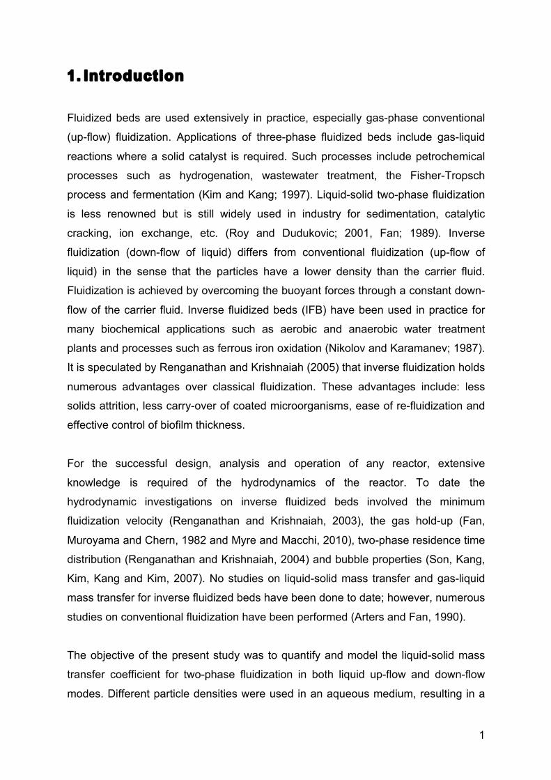
1. Introduction

Fluidized beds are used extensively in practice, especially gas-phase conventional

(up-flow) fluidization. Applications of three-phase fluidized beds include gas-liquid

reactions where a solid catalyst is required. Such processes include petrochemical

processes such as hydrogenation, wastewater treatment, the Fisher-Tropsch

process and fermentation (Kim and Kang; 1997). Liquid-solid two-phase fluidization

is less renowned but is still widely used in industry for sedimentation, catalytic

cracking, ion exchange, etc. (Roy and Dudukovic; 2001, Fan; 1989). Inverse

fluidization (down-flow of liquid) differs from conventional fluidization (up-flow of

liquid) in the sense that the particles have a lower density than the carrier fluid.

Fluidization is achieved by overcoming the buoyant forces through a constant down-

flow of the carrier fluid. Inverse fluidized beds (IFB) have been used in practice for

many biochemical applications such as aerobic and anaerobic water treatment

plants and processes such as ferrous iron oxidation (Nikolov and Karamanev; 1987).

It is speculated by Renganathan and Krishnaiah (2005) that inverse fluidization holds

numerous advantages over classical fluidization. These advantages include: less

solids attrition, less carry-over of coated microorganisms, ease of re-fluidization and

effective control of biofilm thickness.

For the successful design, analysis and operation of any reactor, extensive

knowledge is required of the hydrodynamics of the reactor. To date the

hydrodynamic investigations on inverse fluidized beds involved the minimum

fluidization velocity (Renganathan and Krishnaiah, 2003), the gas hold-up (Fan,

Muroyama and Chern, 1982 and Myre and Macchi, 2010), two-phase residence time

distribution (Renganathan and Krishnaiah, 2004) and bubble properties (Son, Kang,

Kim, Kang and Kim, 2007). No studies on liquid-solid mass transfer and gas-liquid

mass transfer for inverse fluidized beds have been done to date; however, numerous

studies on conventional fluidization have been performed (Arters and Fan, 1990).

The objective of the present study was to quantify and model the liquid-solid mass

transfer coefficient for two-phase fluidization in both liquid up-flow and down-flow

modes. Different particle densities were used in an aqueous medium, resulting in a

2

density difference between the solid and the liquid. A comparison was done between

four different particle types (Δρ   between 410 kg/m3 to 1 300 kg/m3) in order to

determine the effect on liquid-solid mass transfer. These results could then be

compared to a packed bed setup. The effect of a gas-phase inclusion on a

conventional liquid-solid fluidized bed was also investigated in order to compare

liquid-solid mass transfer coefficients between three-phase fluidization and a

conventional liquid-solid fluidization. An increase in reactor performance with an

inclusion of a gas phase was expected, as reported by Arters and Fan (1990).

Experimental work was performed on a novel reactor with external recycling. Liquid-

solid experiments were performed in both up-flow and down-flow mode depending

on the particle density. In addition, three-phase experiments were performed in

concurrent up-flow mode. The dissolution of benzoic acid method was implemented

in order to quantify the liquid-solid mass transfer rate. The liquid-solid mass transfer

coefficient was experimentally determined over a wide range of liquid velocities in

order to investigate bed behaviour. Modelling was done on the data generated in

order to compare the results with the literature correlations and develop new

correlations.

3

2. Transport Parameters Prediction

A survey was done on fluidized bed studies done in literature in order to have a

background on expected fluidization hydrodynamics. As a starting point liquid-solid

conventional fluidized beds will be discussed. Inverse liquid-solid fluidized bed

studies were also investigated in order to examine possible variations from

conventional fluidization. The inclusion of a gas phase to both conventional and

inverse fluidized beds was also investigated. Lastly an investigation was done on all

liquid fluidization liquid-solid mass transfer studies, in order to compile expected

trends along with literature correlations.

2.1 Liquid-solid conventional fluidized bed hydrodynamics

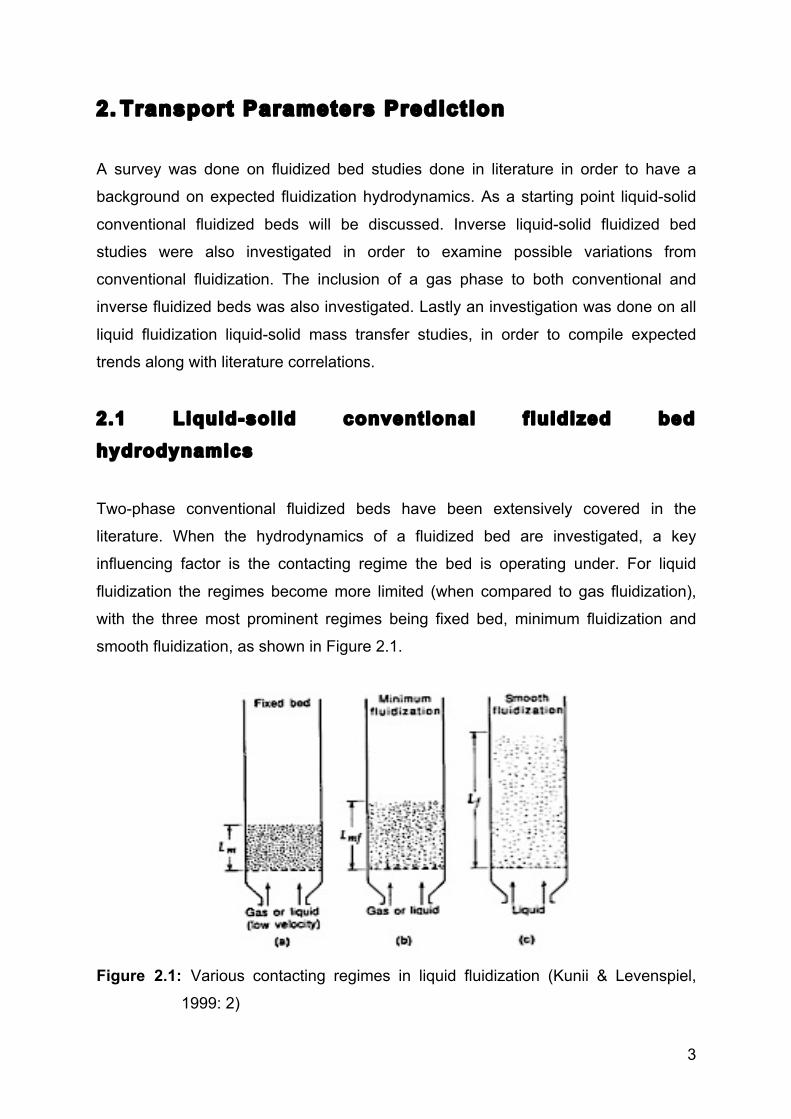
Two-phase conventional fluidized beds have been extensively covered in the

literature. When the hydrodynamics of a fluidized bed are investigated, a key

influencing factor is the contacting regime the bed is operating under. For liquid

fluidization the regimes become more limited (when compared to gas fluidization),

with the three most prominent regimes being fixed bed, minimum fluidization and

smooth fluidization, as shown in Figure 2.1.

Figure 2.1: Various contacting regimes in liquid fluidization (Kunii & Levenspiel,

1999: 2)

4

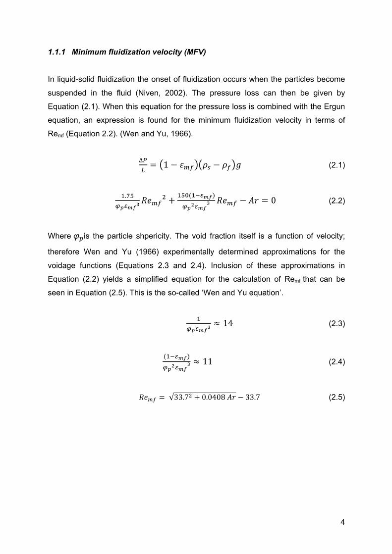
1.1.1 Minimum fluidization velocity (MFV)

In liquid-solid fluidization the onset of fluidization occurs when the particles become

suspended in the fluid (Niven, 2002). The pressure loss can then be given by

Equation (2.1). When this equation for the pressure loss is combined with the Ergun

equation, an expression is found for the minimum fluidization velocity in terms of

Remf (Equation 2.2). (Wen and Yu, 1966).

∆!!= 1 − !!" !! − !! ! (2.1)

!.!"

!!!!"!!"!"! +

!"#(!!!!")

!!!!!"! !"!" − !" = 0 (2.2)

Where !! is the particle shpericity. The void fraction itself is a function of velocity;

therefore Wen and Yu (1966) experimentally determined approximations for the

voidage functions (Equations 2.3 and 2.4). Inclusion of these approximations in

Equation (2.2) yields a simplified equation for the calculation of Remf that can be

seen in Equation (2.5). This is the so-called ‘Wen and Yu equation’.

!

!!!!"!≈ 14 (2.3)

(!!!!")

!!!!!"! ≈ 11 (2.4)

!"!" =   33.7! + 0.0408  !" − 33.7 (2.5)

5

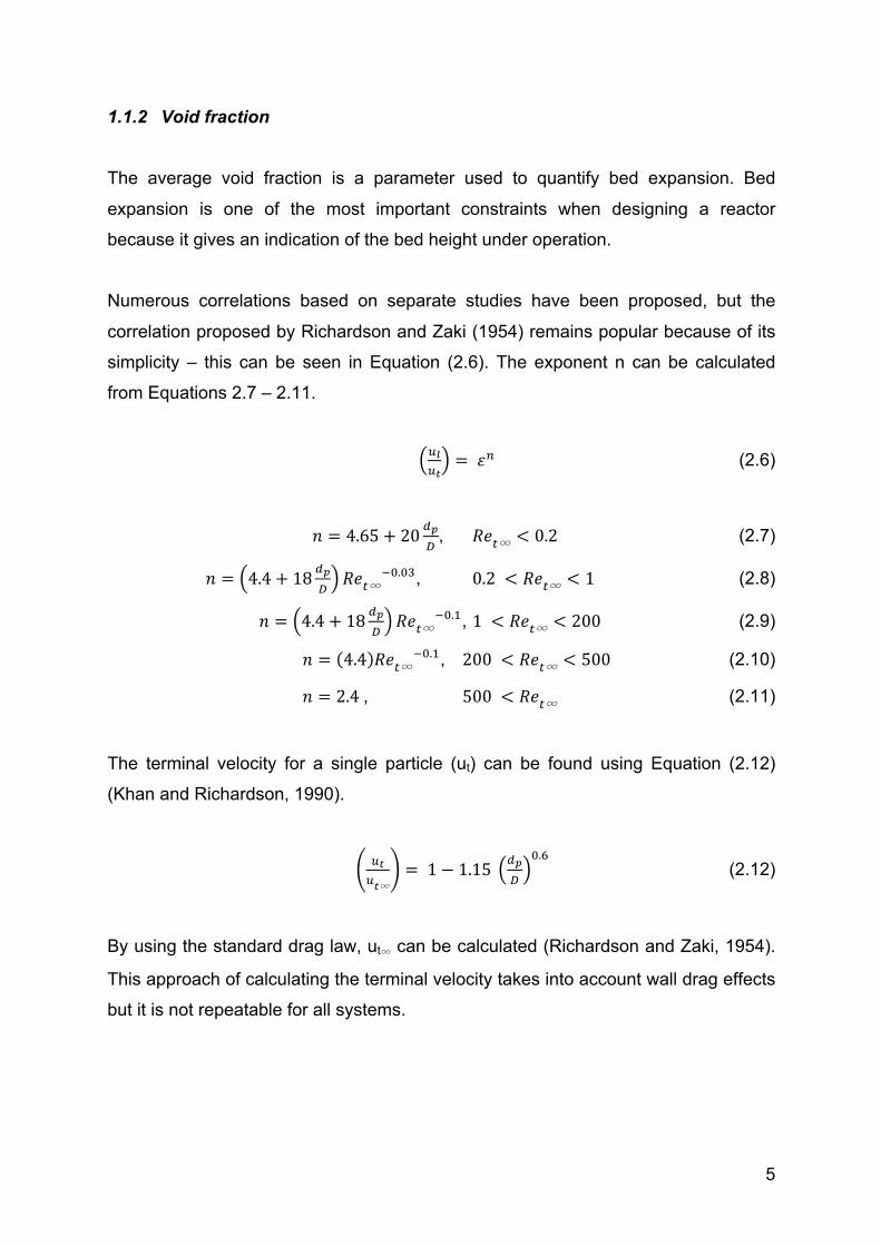
1.1.2 Void fraction

The average void fraction is a parameter used to quantify bed expansion. Bed

expansion is one of the most important constraints when designing a reactor

because it gives an indication of the bed height under operation.

Numerous correlations based on separate studies have been proposed, but the

correlation proposed by Richardson and Zaki (1954) remains popular because of its

simplicity – this can be seen in Equation (2.6). The exponent n can be calculated

from Equations 2.7 – 2.11.

!!!!

=   !! (2.6)

! = 4.65+ 20 !!!

, !"!∞ < 0.2 (2.7)

! = 4.4+ 18 !!!

!"!∞!!.!", 0.2   < !"!∞ < 1 (2.8)

! = 4.4+ 18 !!!

!"!∞!!.!, 1   < !"!∞ < 200 (2.9)

! = 4.4 !"!∞!!.!, 200   < !"!∞ < 500 (2.10)

! = 2.4  , 500   < !"!∞ (2.11)

The terminal velocity for a single particle (ut) can be found using Equation (2.12)

(Khan and Richardson, 1990).

!!!!∞

=  1− 1.15   !!!

!.! (2.12)

By using the standard drag law, ut∞ can be calculated (Richardson and Zaki, 1954).

This approach of calculating the terminal velocity takes into account wall drag effects

but it is not repeatable for all systems.

6

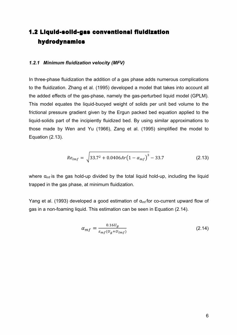
1.2 Liquid-solid-gas conventional fluidization hydrodynamics

1.2.1 Minimum fluidization velocity (MFV)

In three-phase fluidization the addition of a gas phase adds numerous complications

to the fluidization. Zhang et al. (1995) developed a model that takes into account all

the added effects of the gas-phase, namely the gas-perturbed liquid model (GPLM).

This model equates the liquid-buoyed weight of solids per unit bed volume to the

frictional pressure gradient given by the Ergun packed bed equation applied to the

liquid-solids part of the incipiently fluidized bed. By using similar approximations to

those made by Wen and Yu (1966), Zang et al. (1995) simplified the model to

Equation (2.13).

!"!"# =   33.7! + 0.0406!" 1− !!"! − 33.7 (2.13)

where αmf is the gas hold-up divided by the total liquid hold-up, including the liquid

trapped in the gas phase, at minimum fluidization.

Yang et al. (1993) developed a good estimation of αmf for co-current upward flow of

gas in a non-foaming liquid. This estimation can be seen in Equation (2.14).

!!" =!.!"!!

!!"(!!!!!"#) (2.14)

7

1.2.2 Gas hold-up

Fan, Muroyama and Chern (1982) did a study on gas hold-up for two different flow

regimes in inverse fluidized beds. For every superficial gas velocity (Ug0) a gas hold-

up (εg) was measured and documented. They used this data to compile two

empirical equations. These two equations can be seen in Equation (2.15) (inverse

bubbling fluidized bed regime) and Equation (2.16) (inverse slugging fluidized bed

regime).

!!  = 0.322  !!.!"(!!!!!!)!.!" (2.15)

!!  = 2.43  !!!!.!"#!!!!.!" (2.16)

Myre and Macchi (2010) expanded the work done by Fan, Muroyama and Chern

(1982) in order to apply it to a wider range of physical parameters. The authors built

an acrylic column with a height of 2.15 m and a diameter of 0.152 m, which can be

operated as either a bubble column with no particles or as an inverse fluidized bed

with particles in order to determine the effects of gas flow rate, liquid flow rate and

particle loading on the gas hold-up in the column. Myre and Macchi (2010) found that

the gas hold-up decreased with an increase in solids loading. This was attributed to

an increase in bubble coalescence caused by the particles, which means that fewer

micro bubbles are present.

Myre and Macchi (2010) adapted the correlation proposed by Bekish et al. (2006) for

the prediction of gas hold-up. Myre and Macchi (2010) adapted the model by

changing the leading constant parameter from 4.94 x 10-3 to 8.74 x 10-3. The

modified correlation can be seen in Equation (2.17). This modification decreased the

AARE value from 42% to 9%.

!! = 0.00494  !  !  ! (2.17)

With:

8

! =  !!!.!"#!!!.!""

!!!.!"#!!!.!"!!!.!!"

!!!! − !!

!.!"#

! =    !!

!! + 1

!!.!!"

Γ!.!"#

! =    exp  [−2.231!! − 0.157 !!!! − 0.242!!]

Γ = (!!×!!!!!) (2.18)

Where

CV is the volumetric solid concentration in the slurry (v/v),

PT is the total pressure,

Ps is the vapour pressure of the liquid and

DC is the column diameter (m).

The effect of the gas sparger is introduced to the correlation by Γ and can be

calculated by using Equation (2.18), where

Kd is the distributor coefficient,

N0 is the number of orifices in the sparger and

d0 is the diameter of the orifice.

Kd values for perforated plates and multiple-orifice nozzles are 1.364.

1.2.3 Bubble properties

Son, Kang, Kim, Kang and Kim (2007) did a study on bubble size, bubble rise

velocity and bubble frequency in an inverse fluidized bed using a dual electrical

resistivity probe system. These parameters were measured for different liquid

viscosities by using aqueous solutions of carboxyl methyl cellulose (CMC). The

authors used two types of particles, polypropylene and polyethylene, with densities

of 877.3 kg/m3 and 966.6 kg/m3, respectively. The data were generated using a dual

electrical resistivity probe system. The following results were obtained:

9

• The bubble size was correlated using the cord length of the bubbles. It was

found that the cord length increased with an increase in gas velocity. This was

attributed to a higher bubble coalescence, which caused bigger bubble sizes.

The increase in liquid velocity also caused more bubble coalescence because

of the counter-flow of the liquid.

• The authors also noted that the bubble sizes were higher when polypropylene

particles were used than when polyethylene particles were used. A conclusion

was made that the bubble size decreases with increasing fluidized particle

density in inverse fluidized beds.

• The bubble rise velocity increased with an increase in gas velocity or liquid

viscosity, but decreased slightly with an increase in liquid velocity. This was

attributed to the liquid drag on the bubbles.

• The bubble frequency increased with an increase in liquid or gas velocities.

This influenced the gas hold-up in the column. The bubble frequency,

however, decreased with an increase in liquid viscosity.

• The bubble frequency was higher for beds with heavier particles

(polyethylene) than lighter particles (polypropylene).

Son et al. (2007) correlated models for the bubble size (Lv), rising velocity (UB) and

the bubble frequency (FB) using the concept of gas drift flux. These correlations fit

their data, with each equation having a correlation coefficient of between 0.90 and

0.96, and can be seen in Equations (2.19), (2.20) and (2.21) below.

!! = 0.117   !!!!!!!!!

!.!!" !!!!

!!.!"!! !.!"! (2.19)

!! = 0.108   !!!!!!!!!

!!.!"# !!!!

!!.!"!! !.!"# (2.20)

!! = 30.846   !!!!!!!!!

!.!"! !!!!

!.!"#!! !!.!!" (2.21)

10

1.3 Inverse fluidization hydrodynamics

Inverse fluidization differs from classical fluidization in the sense that the particles

have a lower density than the carrier fluid and therefore floats. A continuous

downward flow of liquid then fluidizes the bed. In three-phase fluidization a gas flow

is introduced in a counter flow manner. An inverse fluidized bed can also be run in

liquid batch mode where there is no liquid flow and only upward gas flow through the

liquid and particle bed.

1.3.1 Minimum fluidization velocity

Liquid-solid fluidization

In liquid-solid inverse fluidization, fluidization will commence once the pressure drop

over the reactor is equal to the net buoyant force per unit area. The pressure drop

over the bed is well correlated by the Ergun equation and therefore the MFV can be

determined. Renganathan and Krishnaiah (2003) did a study of all the factors

influencing the minimum fluidization velocity (MFV) in up-flow and down-flow

fluidized beds to determine whether conventional fluidization correlations can be

used for inverse fluidized beds.

To generate experimental data they constructed an inverse fluidized bed and

measured the pressure drop and the void fraction. The MFV was then determined

when the pressure drop and void fraction were plotted against liquid velocity, and an

intersection point was reached between the packed bed regime and fluidized bed

regime. These data were tested against correlations from the literature on

conventional fluidization (Fan et al., 1982; Legile et al, 1992; Nikolov &

Karamanev,1987; Krishnaiah et al., 1993; Ulganathan & Krishnaiah, 1996; Ibrahim et

al., 1996; Biswas & Ganguly, 1997; Calderon et al., 1998; Banerjee et al., 1999;

Buffière & Moletta, 1999; Vijayalakshmi et al., 2000; Cho et al., 2002).

The constant values in the Ergun equation have been determined in the literature by

different authors under different conditions. The correlation found by Wen and Yu

11

(1966) for conventional fluidized beds was deemed the best when compared to the

data compiled by Renganathan and Krishnaiah (2003) with an RMS error of 24 %.

The equation proposed by Wen and Yu (1966) can be seen in Equation (2.22). This

correlation was tested for a variety of particles.

!"!"#! =   33.7! + 0.0408!" − 33.7 (2.22)

From Equation (2.22) the MFV can be calculated, where Relmf0 is the Reynolds

number at minimum fluidization velocity for liquid-solid fluidization, therefore it can be

seen that the conventional Wen and Yu equation can be used, within an acceptable

error, to calculate MFV values for IFB. This equation can be used safely over the

range of Relmf0 = 0.01 to 2000 and Ar = 20 to 70 x 106.

Liquid-solid-gas fluidization

For three-phase inverse fluidization the gas-phase is introduced in a concurrent

manner to the liquid flow. This is different from conventional three-phase fluidized

beds where the gas and liquid flow in a co-current manner. Renganathan and

Krishnaiah (2003) studied three-phase inverse fluidization to see how the results

compare to those of conventional fluidized beds. One of the main differences that the

authors noticed was that the bed fluidizes gradually, unlike two-phase fluidization.

The authors attributed the gradual fluidization to the recirculation of the liquid at the

top of the bed due to the gas flow. This is different from conventional fluidized beds

where the bed is fluidized sharply.

The gas introduced from the bottom of the column adds different effects to the

fluidization. The gas reduces the effective density of the liquid and therefore the

particles become less buoyant. The gas flow also causes liquid circulations in the

liquid phase, which in turn causes an extra drag force on the particles.

Due to the effects discussed above, conventional fluidized bed correlations for the

minimum fluidization velocity cannot be used for inverse fluidized beds.

Renganathan and Krishnaiah (2003) correlated a new empirical equation for the

12

minimum fluidization velocity and tested it against literature correlations. The GPLM

developed by Zhang et al (1995) and discussed in Section 2.2.1, was modified by

Renganathan and Krishnaiah (2003) in order to apply it to inverse fluidized beds.

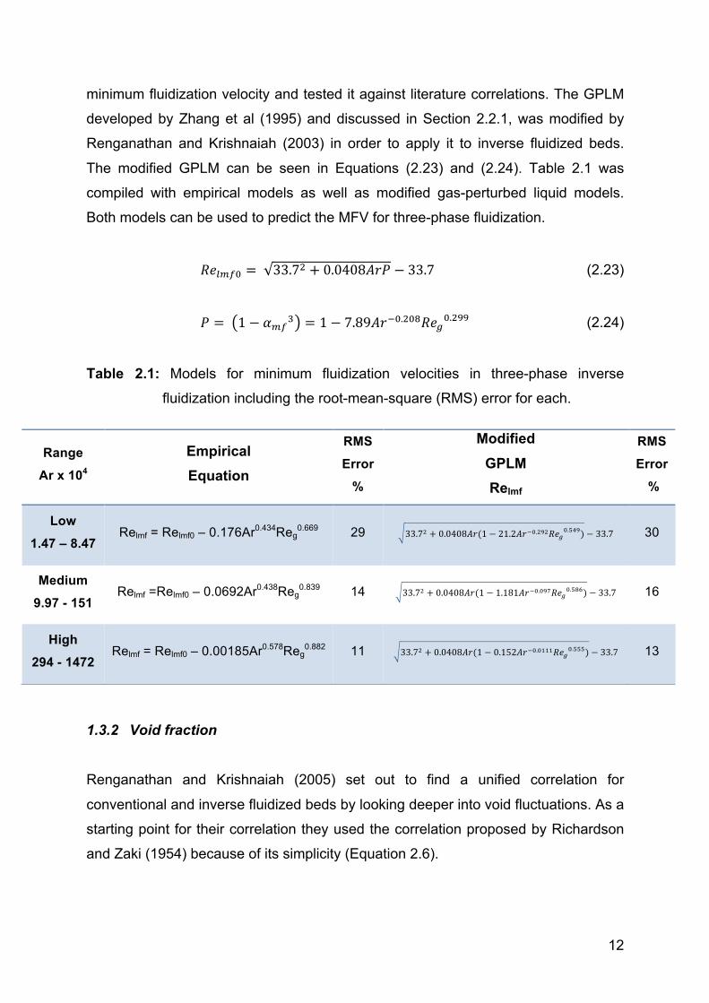
The modified GPLM can be seen in Equations (2.23) and (2.24). Table 2.1 was

compiled with empirical models as well as modified gas-perturbed liquid models.

Both models can be used to predict the MFV for three-phase fluidization.

!"!"#! =   33.7! + 0.0408!"# − 33.7 (2.23)

! =   1− !!"! = 1− 7.89!"!!.!"#!"!!.!"" (2.24)

Table 2.1: Models for minimum fluidization velocities in three-phase inverse

fluidization including the root-mean-square (RMS) error for each.

1.3.2 Void fraction

Renganathan and Krishnaiah (2005) set out to find a unified correlation for

conventional and inverse fluidized beds by looking deeper into void fluctuations. As a

starting point for their correlation they used the correlation proposed by Richardson

and Zaki (1954) because of its simplicity (Equation 2.6).

Range

Ar x 104

Empirical Equation

RMS

Error

%

Modified GPLM Relmf

RMS

Error

%

Low

1.47 – 8.47 Relmf = Relmf0 – 0.176Ar0.434Reg

0.669 29 33.7! + 0.0408!"(1 − 21.2!"!!.!"!!"!!.!"#) − 33.7 30

Medium

9.97 - 151 Relmf =Relmf0 – 0.0692Ar0.438Reg

0.839 14 33.7! + 0.0408!"(1 − 1.181!"!!.!"#!"!!.!"#) − 33.7 16

High

294 - 1472 Relmf = Relmf0 – 0.00185Ar0.578Reg

0.882 11 33.7! + 0.0408!"(1 − 0.152!"!!.!"""!"!!.!!!) − 33.7 13

13

This approach of calculating the terminal velocity takes into account wall drag effects,

but it is not repeatable for all systems. These equations were tested for a number of

experimental data and it was found that the Richardson and Zaki equation works well

if experimental terminal velocities are used but not if Equation (2.12) is used. By

modifying the Turton and Clark (1987) equation for terminal velocity, the overall void

prediction was improved. The equation proposed by Renganathan and Krishnaiah

(2005) can be seen in Equation (2.25). This equation was compared to experimental

terminal velocities and an RMS error of 12% was found.

!∗ =  !"!∗!

!.!!"+   !  ×  !.!"#

!!∗!.!!.!!" !!

!.!!" (2.25)

where u* is the dimensionless terminal velocity in infinite medium, and can be

expressed as Equation (2.26). Similarly d* is the dimensionless particle diameter that

can be calculated using Equation (2.27).

!∗ =  !!∞!!!

!!!  (!!!!!)

!! (2.26)

!∗ =  !!!!!  (!!!!!)

!!!

!! (2.27)

1.3.3 Liquid mixing (dispersion)

RTD (Residence time distribution) studies have been done by Renganathan and

Krishnaiah (2004) on a two-phase IFB in order to quantify the extent of mixing in

these reactors. It is to be expected that the extent of mixing will be higher when the

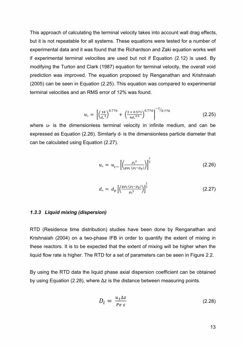
liquid flow rate is higher. The RTD for a set of parameters can be seen in Figure 2.2.

By using the RTD data the liquid phase axial dispersion coefficient can be obtained

by using Equation (2.28), where Δz is the distance between measuring points.

!! =  !!∆!!"  !

(2.28)

14

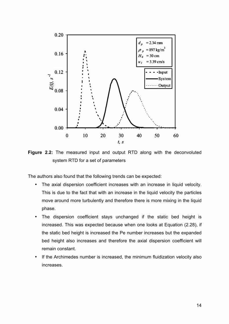
Figure 2.2: The measured input and output RTD along with the deconvoluted

system RTD for a set of parameters

The authors also found that the following trends can be expected:

• The axial dispersion coefficient increases with an increase in liquid velocity.

This is due to the fact that with an increase in the liquid velocity the particles

move around more turbulently and therefore there is more mixing in the liquid

phase.

• The dispersion coefficient stays unchanged if the static bed height is

increased. This was expected because when one looks at Equation (2.28), if

the static bed height is increased the Pe number increases but the expanded

bed height also increases and therefore the axial dispersion coefficient will

remain constant.

• If the Archimedes number is increased, the minimum fluidization velocity also

increases.

15

In their experiments, Renganathan and Krishnaiah (2004) found a correlation for the

axial dispersion coefficient that can be seen in Equation (2.29). When compared to

experimental data, an RMS error of 28% was found. This correlation is only valid for

17.6 < Ar < 1.47 x 107 and 0.036 < Re < 1 267.

!! = 1.48  ×  10!!!"!.!! !"!"!"

!.!" (2.29)

1.4 Liquid-solid mass transfer in two- and three-phase fluidized beds

In any fluidized bed, whether liquid-solid or liquid-solid-gas, liquid-solid mass transfer

can become a limiting step, especially for larger particle sizes. For this reason proper

prediction of the liquid-solid mass transfer is needed for a proper reactor design. In

order to predict the mass transfer coefficient all the factors influencing mass transfer

must be investigated and understood.

According to Arters and Fan (1990) and numerous other references, the following

trends can be expected in a conventional fluidized bed:

• The liquid velocity has no effect on the liquid-solid mass transfer coefficient for

fully fluidized beds. This is observed in both two- and three-phase fluidization.

(Hassanien et al., 1984; Arters and Fan, 1986; Prakash et al., 1987)

• The mass transfer coefficient increases at near-minimum fluidization liquid

velocities. (Nikov and Delmas, 1987).

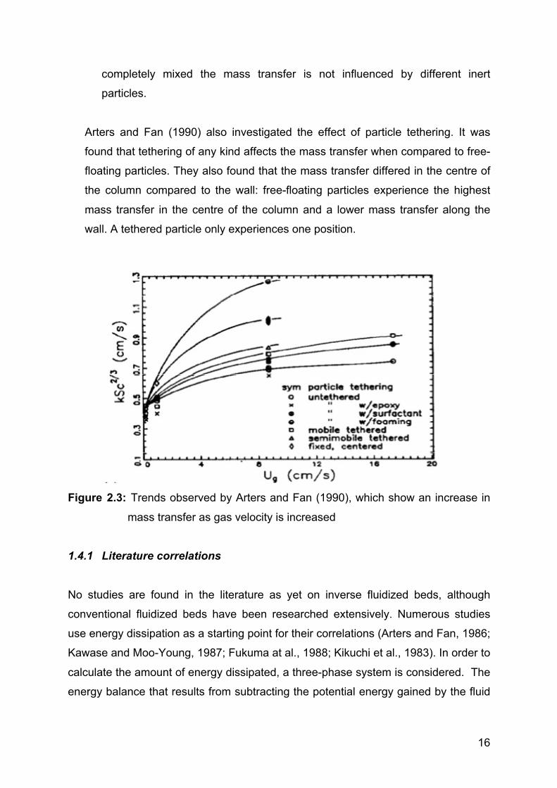
• The mass transfer is further increased as gas is introduced. This positive

effect on the mass transfer tails off at higher gas velocities. These trends can

be seen in Figure 2.3.

• The effect of the changing gas hold-up, because of the surfactant effect of

benzoic acid, was found to have less than 15% effect on the mass transfer

coefficient under normal operating conditions.

• When the effect of different inert particles was investigated it was found that

when all the active and inert particles (with the same physical properties) are

16

completely mixed the mass transfer is not influenced by different inert

particles.

Arters and Fan (1990) also investigated the effect of particle tethering. It was

found that tethering of any kind affects the mass transfer when compared to free-

floating particles. They also found that the mass transfer differed in the centre of

the column compared to the wall: free-floating particles experience the highest

mass transfer in the centre of the column and a lower mass transfer along the

wall. A tethered particle only experiences one position.

Figure 2.3: Trends observed by Arters and Fan (1990), which show an increase in

mass transfer as gas velocity is increased

1.4.1 Literature correlations

No studies are found in the literature as yet on inverse fluidized beds, although

conventional fluidized beds have been researched extensively. Numerous studies

use energy dissipation as a starting point for their correlations (Arters and Fan, 1986;

Kawase and Moo-Young, 1987; Fukuma at al., 1988; Kikuchi et al., 1983). In order to

calculate the amount of energy dissipated, a three-phase system is considered. The

energy balance that results from subtracting the potential energy gained by the fluid

17

phase from the total energy input into the system, is given by Equation (2.30) (Arters

and Fan, 1990):

! =  !!"#!!"#! !! + !! !!!! + !!!! + !!!! − !!"!!!"#! !!!! + !!!! (2.30)

Equation (2.30) can be simplified to Equation (2.31) using the following

simplifications:

!! ≪ !! ,!!

!! =  !!"#!!"#!!!!

! =  ! !! + !! !!!! + !!!! − !!!! /(!!!!) (2.31)

where e is the rate of energy dissipated per unit mass of liquid. Other studies use a

less rigorous method as proposed by Fukuma et al. (1988) of determining the energy

dissipated by considering the individual energy effects of the particles and the

bubbles, including wall friction. Arters and Fan (1990) found this method to be just an

approximation of the dissipation energy, and the method described in Equation

(2.31) was found to be more accurate.

Numerous correlations found in the literature that use energy dissipation have a

standard form that can be seen in Equation (2.32).

!ℎ =  !(!!!!

!!)!!"! (2.32)

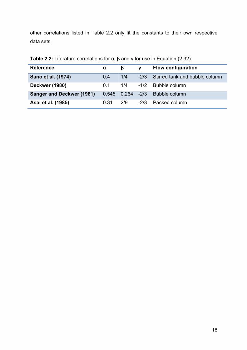
Some of the correlations using the energy dissipation approach to mass transfer are

listed in Table 2.2 with the experimentally determined constants for α, β and γ.

Kawase and Moo-Young (1987) used a combination of the Kolmogoroff theory and

the Levich three-zone model to theoretically derive a correlation to determine the

liquid-solid mass transfer coefficient. They found the constants α, β and γ to be

0.162, 0.24 and 1/3 respectively. The constants proposed by Kawase and Moo-

Young (1987) are preferred because they were derived theoretically, whereas the

18

other correlations listed in Table 2.2 only fit the constants to their own respective

data sets.

Table 2.2: Literature correlations for α, β and γ for use in Equation (2.32)

Reference α β γ Flow configuration

Sano et al. (1974) 0.4 1/4 -2/3 Stirred tank and bubble column

Deckwer (1980) 0.1 1/4 -1/2 Bubble column

Sanger and Deckwer (1981) 0.545 0.264 -2/3 Bubble column

Asai et al. (1985) 0.31 2/9 -2/3 Packed column

19

3. Experimental

3.1 Apparatus

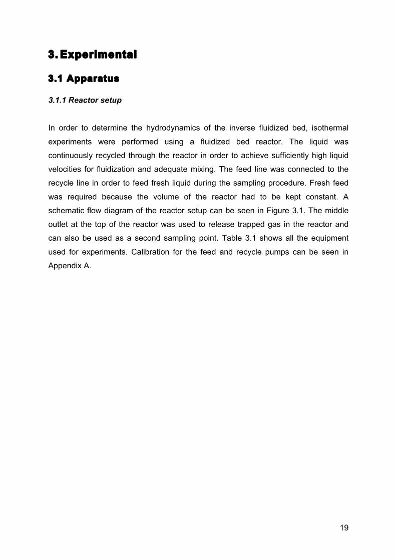
3.1.1 Reactor setup

In order to determine the hydrodynamics of the inverse fluidized bed, isothermal

experiments were performed using a fluidized bed reactor. The liquid was

continuously recycled through the reactor in order to achieve sufficiently high liquid

velocities for fluidization and adequate mixing. The feed line was connected to the

recycle line in order to feed fresh liquid during the sampling procedure. Fresh feed

was required because the volume of the reactor had to be kept constant. A

schematic flow diagram of the reactor setup can be seen in Figure 3.1. The middle

outlet at the top of the reactor was used to release trapped gas in the reactor and

can also be used as a second sampling point. Table 3.1 shows all the equipment

used for experiments. Calibration for the feed and recycle pumps can be seen in

Appendix A.

20

Table 3.1: List off all equipment used in experiments and shown in Figure 3.1

Number Equipment Description E-1 CO2 cylinder African Oxygen - Technical E-2 Heat plate Heidolph Instruments - MR Hei standard E-3 Reactor vessel Custom made (Figure 3.2) E-4 Peristaltic pump Watson Merlow 520S E-5 Peristaltic pump Watson Merlow 520S E-6 Peristaltic pump Watson Merlow 323 E-7 Feed tank L-1 Gas input line L-2 Sample line L-3 Gas exit line L-4 Recycle line L-5 Feed line P-1 Pressure regulator African Oxygen - Afrox Scientific T-1 Temperature controller Connected to heat plate - see E-2 V-1 Plug valve Swagelok - P4T series V-2 Needle valve Swagelok - S series

Figure 3.1: A schematic flow diagram of the reactor setup used in all experiments

21

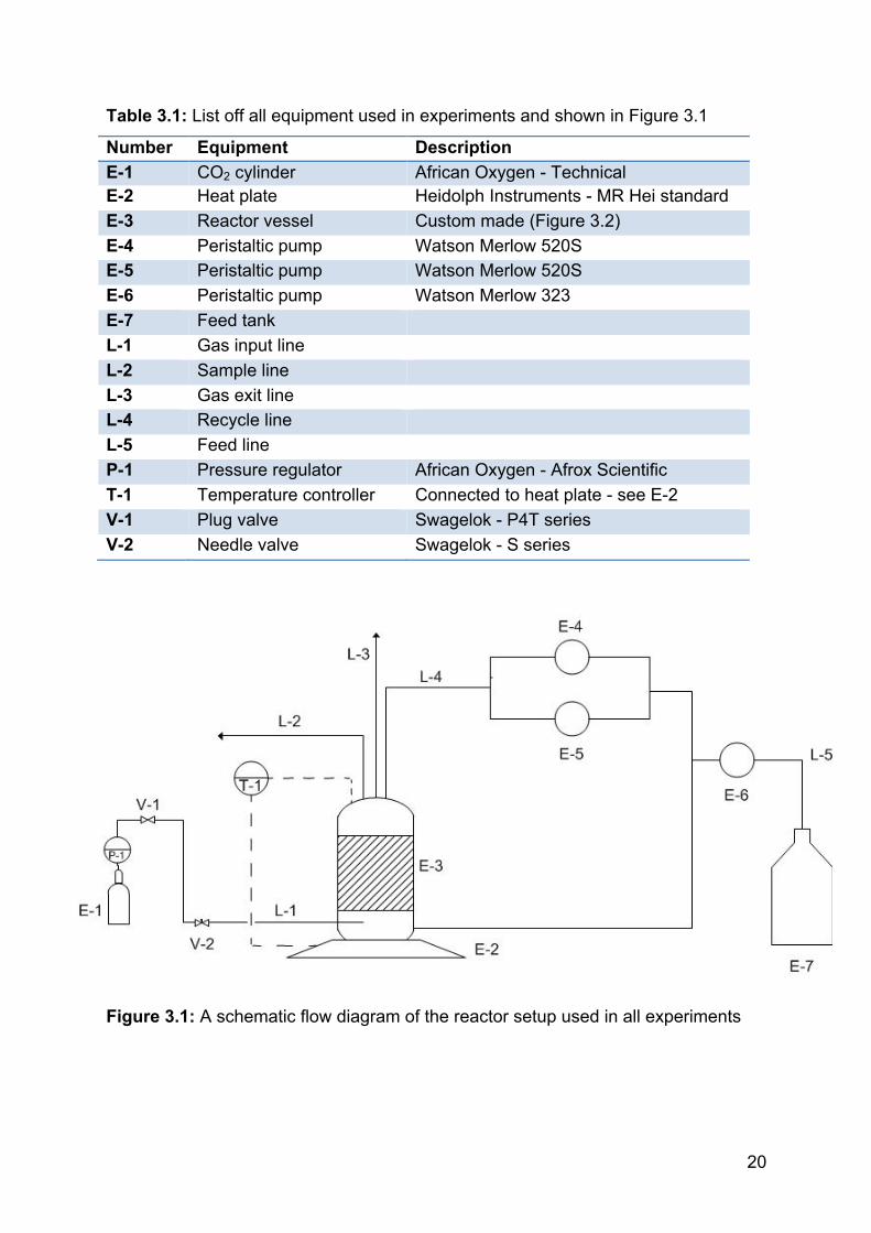
The reactor vessel used was constructed so that it could be run either up-flow

(conventional fluidization) or down-flow (inverse fluidization). Two aluminium liquid

distributors were added, one at the top and one at the bottom. An acrylic tube was

chosen as the housing of the bed because of its visibility and durability. Four O-rings

were added to the top and bottom parts of the reactor to achieve a watertight seal.

The temperature was kept at 30 °C (±1 °C) for all the experiments, controlled via the

hot plate. A representation of the reactor can be seen in Figure 3.2. Photographs of

the reactor dissembled and assembled are shown in Figure 3.3.

Figure 3.2: Representation of the fluidized bed reactor used in all experiments

Top liquid

distributor

110 mm

Bottom liquid

distributor

Gas distributor

Gas feed line

5 ports to

reactor

Liquid in/out line

68 mm

37 mm

Settling zone

22

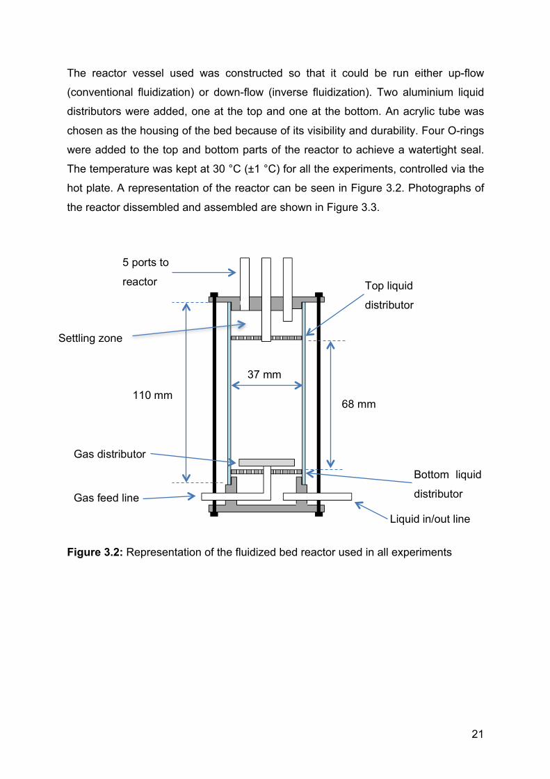
Figure 3.3: Photos of the reactor a) assembled and b) disassembled (with two

different gas distributor designs)

The reactor can also be run in either liquid-solid or three-phase modes. The detail

design of the liquid distributor can be seen in Figure 3.4. For three-phase fluidization

only up-flow was possible because counter-current flow with liquid down-flow creates

a pressure differential over the top liquid distributer that complicates operation.

Photographs of Poraver (low density) and alumina (high density) particles being

fluidized can be seen in Figure 3.5.

a) b)

23

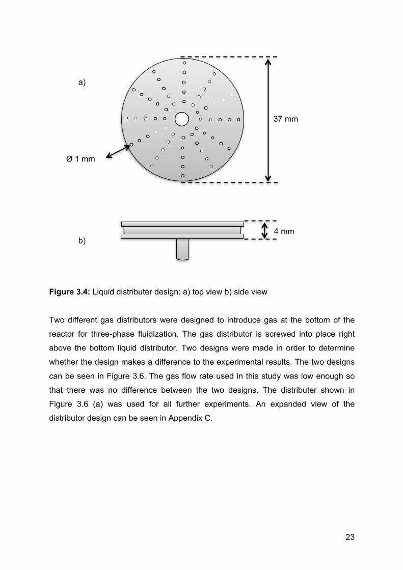
Figure 3.4: Liquid distributer design: a) top view b) side view

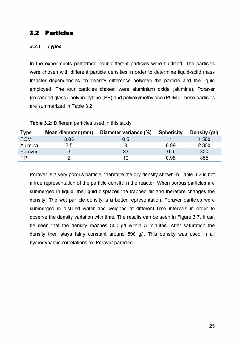
Two different gas distributors were designed to introduce gas at the bottom of the

reactor for three-phase fluidization. The gas distributor is screwed into place right

above the bottom liquid distributor. Two designs were made in order to determine

whether the design makes a difference to the experimental results. The two designs

can be seen in Figure 3.6. The gas flow rate used in this study was low enough so

that there was no difference between the two designs. The distributer shown in

Figure 3.6 (a) was used for all further experiments. An expanded view of the

distributor design can be seen in Appendix C.

37 mm

Ø 1 mm

4 mm

a)

b)

24

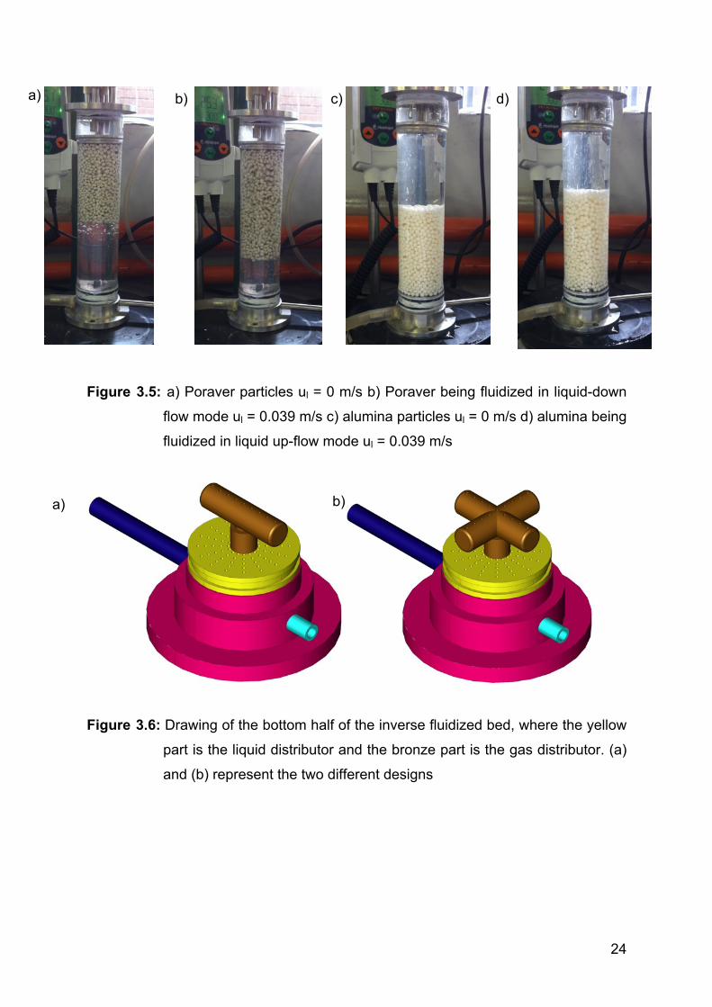
Figure 3.5: a) Poraver particles ul = 0 m/s b) Poraver being fluidized in liquid-down

flow mode ul = 0.039 m/s c) alumina particles ul = 0 m/s d) alumina being

fluidized in liquid up-flow mode ul = 0.039 m/s

Figure 3.6: Drawing of the bottom half of the inverse fluidized bed, where the yellow

part is the liquid distributor and the bronze part is the gas distributor. (a)

and (b) represent the two different designs

a) c)

b) a)

b) d)

25

3.2 Particles

3.2.1 Types

In the experiments performed, four different particles were fluidized. The particles

were chosen with different particle densities in order to determine liquid-solid mass

transfer dependencies on density difference between the particle and the liquid

employed. The four particles chosen were aluminium oxide (alumina), Poraver

(expanded glass), polypropylene (PP) and polyoxymethylene (POM). These particles

are summarized in Table 3.2.

Table 3.2: Different particles used in this study

Type Mean diameter (mm) Diameter variance (%) Sphericity Density (g/l) POM 3.85 0.5 1 1 580 Alumina 3.5 8 0.99 2 300 Poraver 3 33 0.9 320 PP 2 10 0.98 855

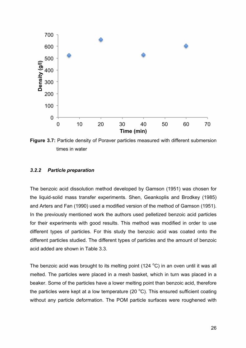
Poraver is a very porous particle, therefore the dry density shown in Table 3.2 is not

a true representation of the particle density in the reactor. When porous particles are

submerged in liquid, the liquid displaces the trapped air and therefore changes the

density. The wet particle density is a better representation. Poraver particles were

submerged in distilled water and weighed at different time intervals in order to

observe the density variation with time. The results can be seen in Figure 3.7. It can

be seen that the density reaches 550 g/l within 3 minutes. After saturation the

density then stays fairly constant around 590 g/l. This density was used in all

hydrodynamic correlations for Poraver particles.

26

Figure 3.7: Particle density of Poraver particles measured with different submersion

times in water

3.2.2 Particle preparation

The benzoic acid dissolution method developed by Gamson (1951) was chosen for

the liquid-solid mass transfer experiments. Shen, Geankoplis and Brodkey (1985)

and Arters and Fan (1990) used a modified version of the method of Gamson (1951).

In the previously mentioned work the authors used pelletized benzoic acid particles

for their experiments with good results. This method was modified in order to use

different types of particles. For this study the benzoic acid was coated onto the

different particles studied. The different types of particles and the amount of benzoic

acid added are shown in Table 3.3.

The benzoic acid was brought to its melting point (124 oC) in an oven until it was all

melted. The particles were placed in a mesh basket, which in turn was placed in a

beaker. Some of the particles have a lower melting point than benzoic acid, therefore

the particles were kept at a low temperature (20 oC). This ensured sufficient coating

without any particle deformation. The POM particle surfaces were roughened with

0

100

200

300

400

500

600

700

0 10 20 30 40 50 60 70

Den

sity

(g/l)

Time (min)

27

sandpaper to ensure proper adhesion of the benzoic acid. The results of the coating

procedure can be seen in Table 3.3.

Table 3.3: Different particles coated with the amount of benzoic acid (BA) added

Type Diameter (mm)

BA (x103 g) coated per

particle

Number of particles used per experiment

Total external area of

particles (x103m3)

Total mass BA added (g) per experiment

Alumina 3.5 10.42 33 1.269 0.344 Poraver 3 3.79 44 1.244 0.167

PP 2.4 5.24 70 1.267 0.367 POM 3.85 25.75 27 1.257 0.695

3.3 Data interpretation

The boundary layer theory is used to describe the liquid solid mass transfer. It is

based on a stagnant film of fluid that is formed around the particle. Because of the

stagnant film of fluid that is formed around a catalyst pellet diffusion through this

stagnant film is needed. The bulk concentration of a species will not be the

concentration that the active site on the catalyst surface will see. If it is assumed that

the properties like temperature and concentration at the edge of the film are the

same as the bulk fluid of thickness δ, then the flux through the film can be described

by the following equation (Fogler, 2009:773):

   !! =!!"!   . [!!" − !!"] (3.1)

Where CAb and CAs are the concentrations of species A in the bulk and surface

respectively. The ratio between the diffusivity DAB to the thickness of the film δ is

called the mass transfer coefficient, kc. Then the reaction rate due to mass transfer

becomes:

!!\!" = !!!  . [!!" − !!"] (3.2)

In order to determine the mass transfer coefficient from the dissolution method, the

reaction rate is written in terms of reactor volume to give Equation (3.3).

28

!!!"!"

= !!!!  .[!!"#  !  !!"]!

(3.3)

Where

as is the total external area of the coated particles,

V is the reactor volume,

CAb is the concentration of benzoic acid in the bulk fluid and

Csat is the saturation concentration of benzoic acid.

The saturation concentration of benzoic acid in water was experimentally determined

at 30 oC to be 5.64 g/l. The result obtained compares well with the values obtained

by Delgado (2006) and Qing-Zhu et al. (2006). For all the experiments the area of

the particles was kept the same in order to compare results (see Table 3.3).

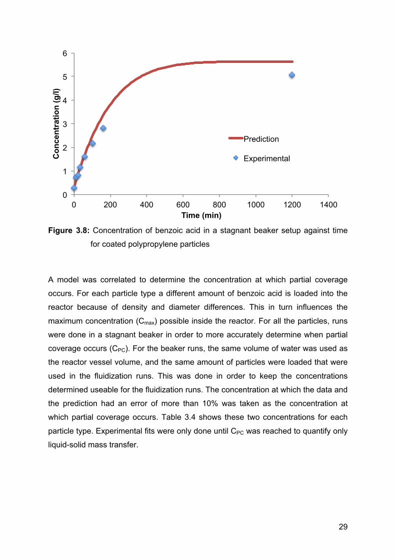
Since the thickness of the benzoic acid layer varied substantially, the dissolution

experiments resulted in partial depletion of benzoic acid on sections of the particle

surface. To ensure proper quantification of the specific mass transfer coefficient, only

the initial dissolution data were considered where the particles are still fully covered

by benzoic acid. This can be seen in Figure 3.8. The model prediction continues until

saturation is reached. In the experiments this saturation concentration was never

reached because only a limited amount of benzoic acid is available to dissolve.

29

Figure 3.8: Concentration of benzoic acid in a stagnant beaker setup against time

for coated polypropylene particles

A model was correlated to determine the concentration at which partial coverage

occurs. For each particle type a different amount of benzoic acid is loaded into the

reactor because of density and diameter differences. This in turn influences the

maximum concentration (Cmax) possible inside the reactor. For all the particles, runs

were done in a stagnant beaker in order to more accurately determine when partial

coverage occurs (CPC). For the beaker runs, the same volume of water was used as

the reactor vessel volume, and the same amount of particles were loaded that were

used in the fluidization runs. This was done in order to keep the concentrations

determined useable for the fluidization runs. The concentration at which the data and

the prediction had an error of more than 10% was taken as the concentration at

which partial coverage occurs. Table 3.4 shows these two concentrations for each

particle type. Experimental fits were only done until CPC was reached to quantify only

liquid-solid mass transfer.

0

1

2

3

4

5

6

0 200 400 600 800 1000 1200 1400

Con

cent

ratio

n (g

/l)

Time (min)

Prediction

Experimental

30

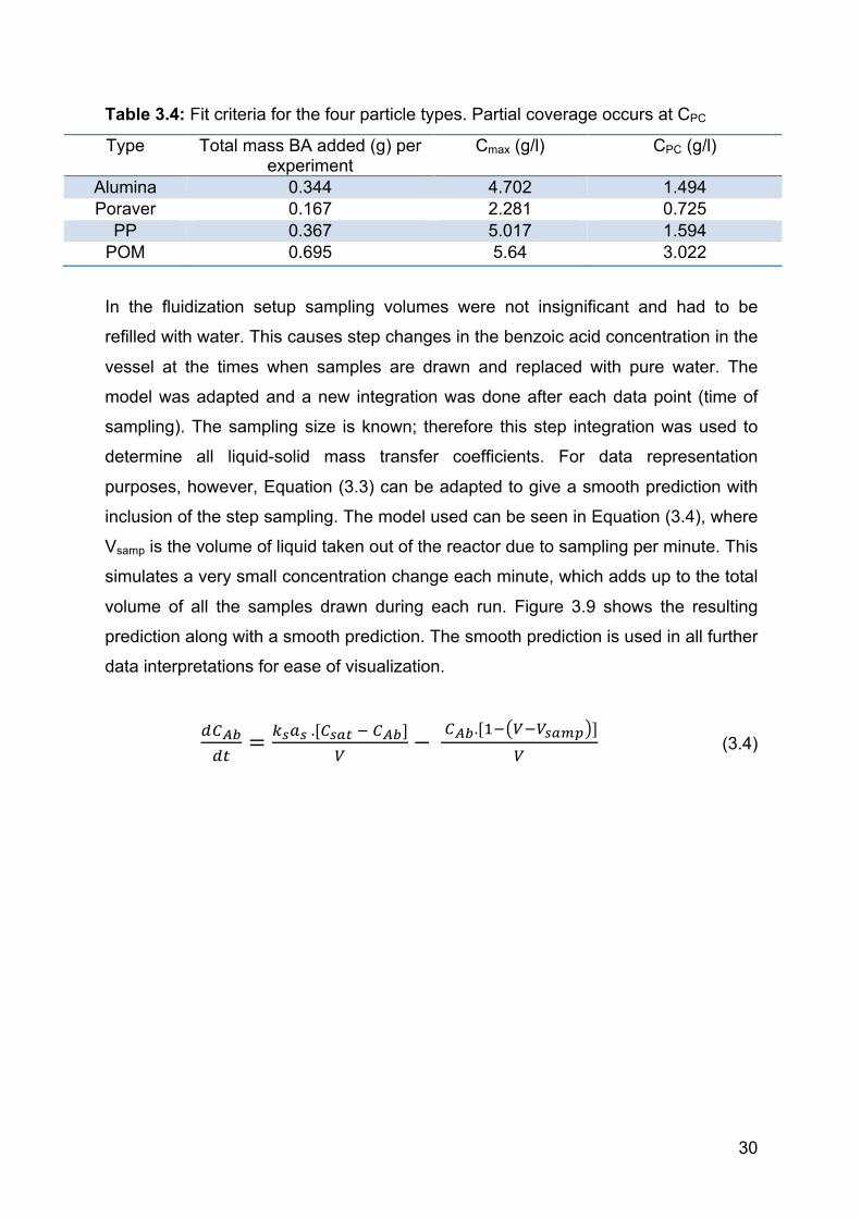
Table 3.4: Fit criteria for the four particle types. Partial coverage occurs at CPC

Type Total mass BA added (g) per experiment

Cmax (g/l) CPC (g/l)

Alumina 0.344 4.702 1.494 Poraver 0.167 2.281 0.725

PP 0.367 5.017 1.594 POM 0.695 5.64 3.022

In the fluidization setup sampling volumes were not insignificant and had to be

refilled with water. This causes step changes in the benzoic acid concentration in the

vessel at the times when samples are drawn and replaced with pure water. The

model was adapted and a new integration was done after each data point (time of

sampling). The sampling size is known; therefore this step integration was used to

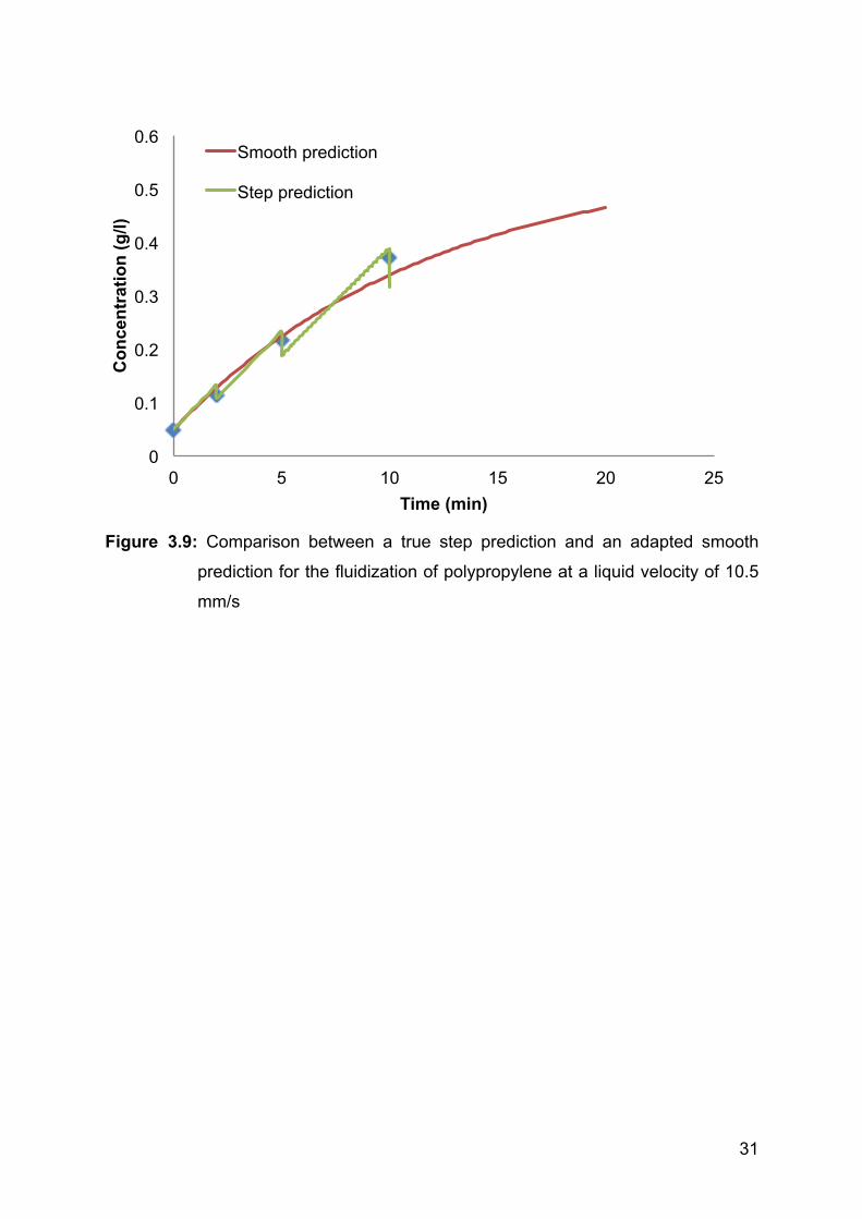
determine all liquid-solid mass transfer coefficients. For data representation

purposes, however, Equation (3.3) can be adapted to give a smooth prediction with

inclusion of the step sampling. The model used can be seen in Equation (3.4), where

Vsamp is the volume of liquid taken out of the reactor due to sampling per minute. This

simulates a very small concentration change each minute, which adds up to the total

volume of all the samples drawn during each run. Figure 3.9 shows the resulting

prediction along with a smooth prediction. The smooth prediction is used in all further

data interpretations for ease of visualization.

!!!"!"

= !!!!  .[!!"#  !  !!"]!

−    !!".[!! !!!!"#$ ]!

(3.4)

31

Figure 3.9: Comparison between a true step prediction and an adapted smooth

prediction for the fluidization of polypropylene at a liquid velocity of 10.5

mm/s

0

0.1

0.2

0.3

0.4

0.5

0.6

0 5 10 15 20 25

Con

cent

ratio

n (g

/l)

Time (min)

Smooth prediction

Step prediction

32

4. Results and discussions

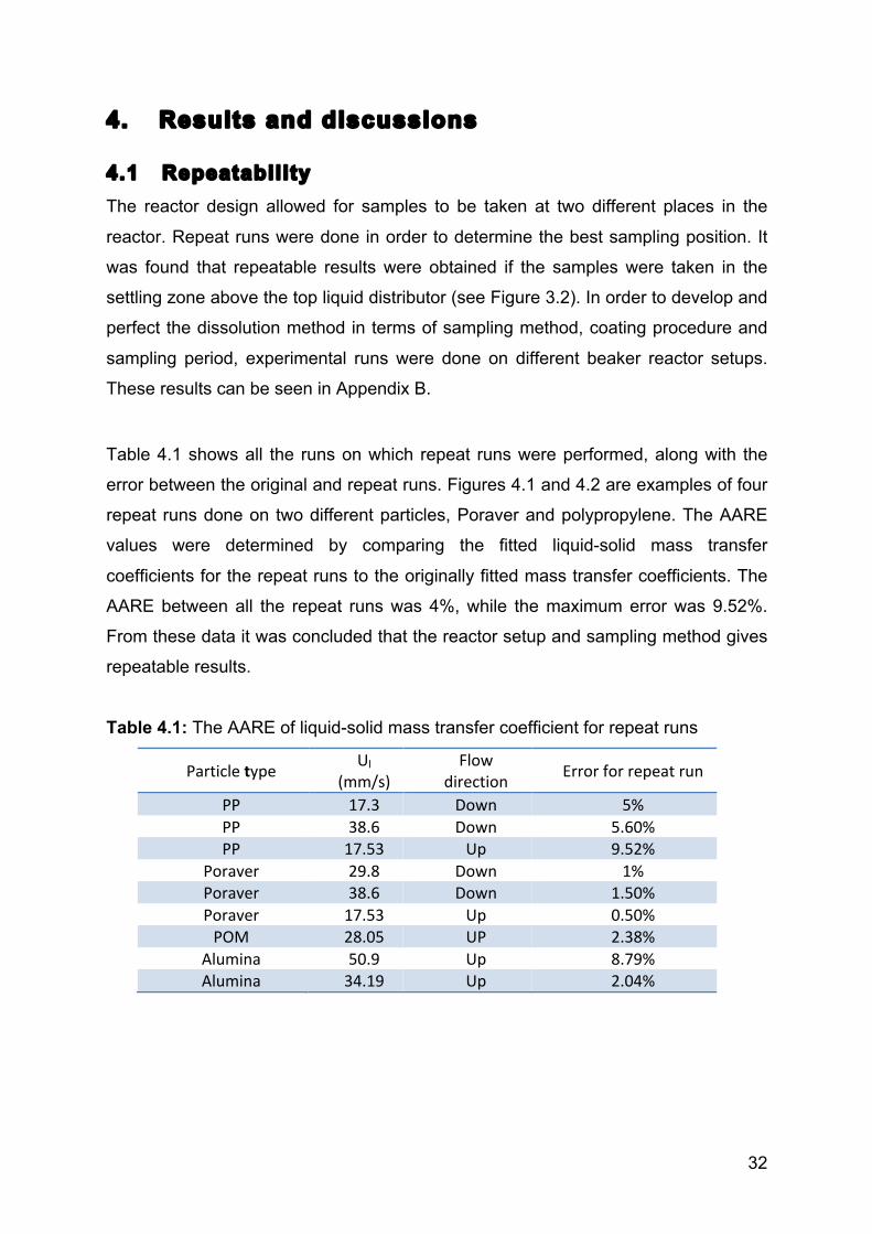
4.1 Repeatability The reactor design allowed for samples to be taken at two different places in the

reactor. Repeat runs were done in order to determine the best sampling position. It

was found that repeatable results were obtained if the samples were taken in the

settling zone above the top liquid distributor (see Figure 3.2). In order to develop and

perfect the dissolution method in terms of sampling method, coating procedure and

sampling period, experimental runs were done on different beaker reactor setups.

These results can be seen in Appendix B.

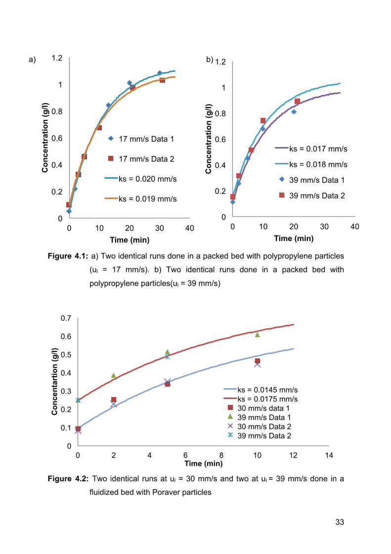
Table 4.1 shows all the runs on which repeat runs were performed, along with the

error between the original and repeat runs. Figures 4.1 and 4.2 are examples of four

repeat runs done on two different particles, Poraver and polypropylene. The AARE

values were determined by comparing the fitted liquid-solid mass transfer

coefficients for the repeat runs to the originally fitted mass transfer coefficients. The

AARE between all the repeat runs was 4%, while the maximum error was 9.52%.

From these data it was concluded that the reactor setup and sampling method gives

repeatable results.

Table 4.1: The AARE of liquid-solid mass transfer coefficient for repeat runs

Particle  type   Ul  (mm/s)  

Flow  direction   Error  for  repeat  run  

PP   17.3   Down   5%  PP   38.6   Down   5.60%  PP   17.53   Up   9.52%  

Poraver   29.8   Down   1%  Poraver   38.6   Down   1.50%  Poraver   17.53   Up   0.50%  POM   28.05   UP   2.38%  

Alumina   50.9   Up   8.79%  Alumina   34.19   Up   2.04%  

33

Figure 4.1: a) Two identical runs done in a packed bed with polypropylene particles

(ul = 17 mm/s). b) Two identical runs done in a packed bed with

polypropylene particles(ul = 39 mm/s)

Figure 4.2: Two identical runs at ul = 30 mm/s and two at ul = 39 mm/s done in a

fluidized bed with Poraver particles

0

0.2

0.4

0.6

0.8

1

1.2

0 10 20 30 40

Con

cent

ratio

n (g

/l)

Time (min)

17 mm/s Data 1

17 mm/s Data 2

ks = 0.020 mm/s

ks = 0.019 mm/s

0

0.2

0.4

0.6

0.8

1

1.2

0 10 20 30 40

Con

cent

ratio

n (g

/l)

Time (min)

ks = 0.017 mm/s

ks = 0.018 mm/s

39 mm/s Data 1

39 mm/s Data 2

0

0.1

0.2

0.3

0.4

0.5

0.6

0.7

0 2 4 6 8 10 12 14

Con

cent

artio

n (g

/l)

Time (min)

ks = 0.0145 mm/s ks = 0.0175 mm/s 30 mm/s data 1 39 mm/s Data 1 30 mm/s Data 2 39 mm/s Data 2

a) b)

34

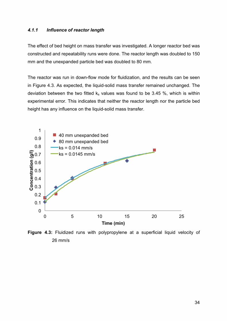
4.1.1 Influence of reactor length

The effect of bed height on mass transfer was investigated. A longer reactor bed was

constructed and repeatability runs were done. The reactor length was doubled to 150

mm and the unexpanded particle bed was doubled to 80 mm.

The reactor was run in down-flow mode for fluidization, and the results can be seen

in Figure 4.3. As expected, the liquid-solid mass transfer remained unchanged. The

deviation between the two fitted ks values was found to be 3.45 %, which is within

experimental error. This indicates that neither the reactor length nor the particle bed

height has any influence on the liquid-solid mass transfer.

Figure 4.3: Fluidized runs with polypropylene at a superficial liquid velocity of

26 mm/s

0

0.1

0.2

0.3

0.4

0.5

0.6

0.7

0.8

0.9

1

0 5 10 15 20 25

Con

cent

ratio

n (g

/l)

Time (min)

40 mm unexpanded bed 80 mm unexpanded bed ks = 0.014 mm/s ks = 0.0145 mm/s

35

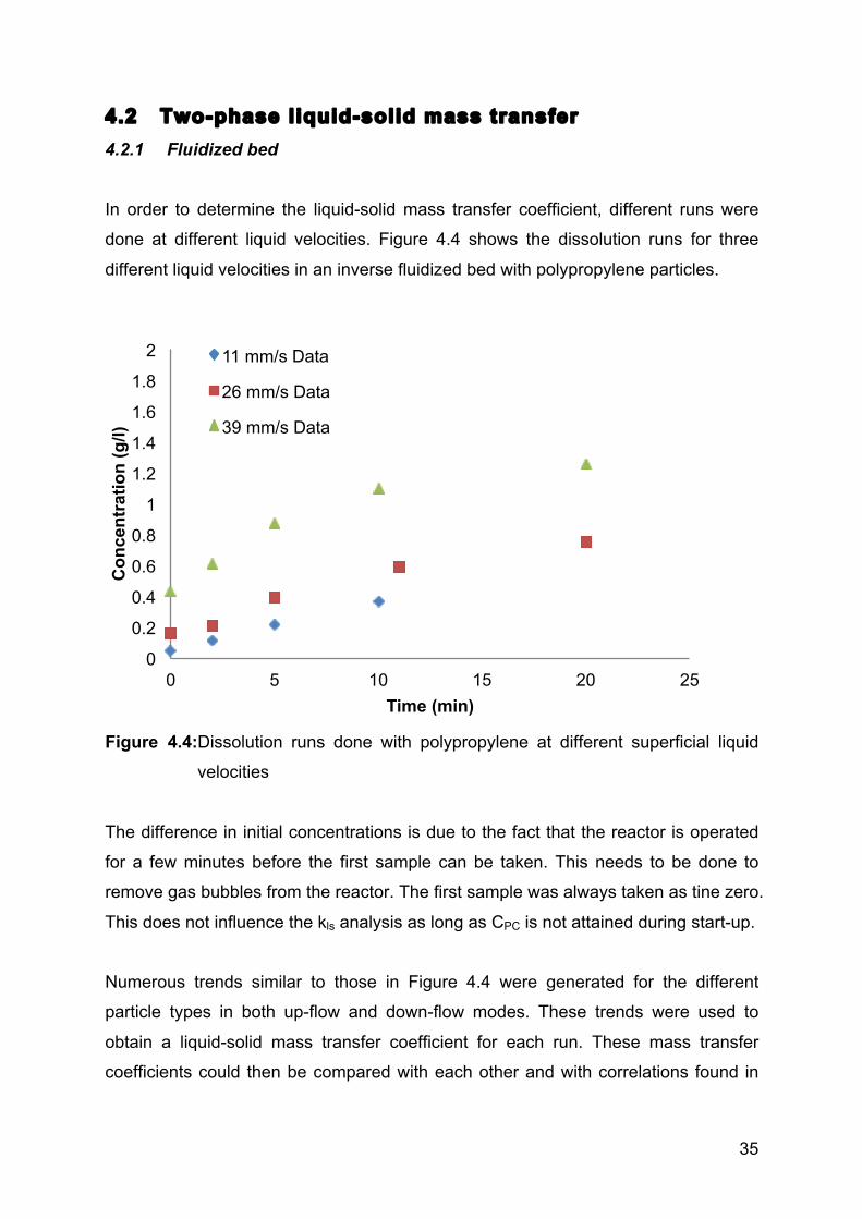
4.2 Two-phase liquid-solid mass transfer 4.2.1 Fluidized bed

In order to determine the liquid-solid mass transfer coefficient, different runs were

done at different liquid velocities. Figure 4.4 shows the dissolution runs for three

different liquid velocities in an inverse fluidized bed with polypropylene particles.

Figure 4.4:Dissolution runs done with polypropylene at different superficial liquid

velocities

The difference in initial concentrations is due to the fact that the reactor is operated

for a few minutes before the first sample can be taken. This needs to be done to

remove gas bubbles from the reactor. The first sample was always taken as tine zero.

This does not influence the kls analysis as long as CPC is not attained during start-up.

Numerous trends similar to those in Figure 4.4 were generated for the different

particle types in both up-flow and down-flow modes. These trends were used to

obtain a liquid-solid mass transfer coefficient for each run. These mass transfer

coefficients could then be compared with each other and with correlations found in

0

0.2

0.4

0.6

0.8

1

1.2

1.4

1.6

1.8

2

0 5 10 15 20 25

Con

cent

ratio

n (g

/l)

Time (min)

11 mm/s Data

26 mm/s Data

39 mm/s Data

36

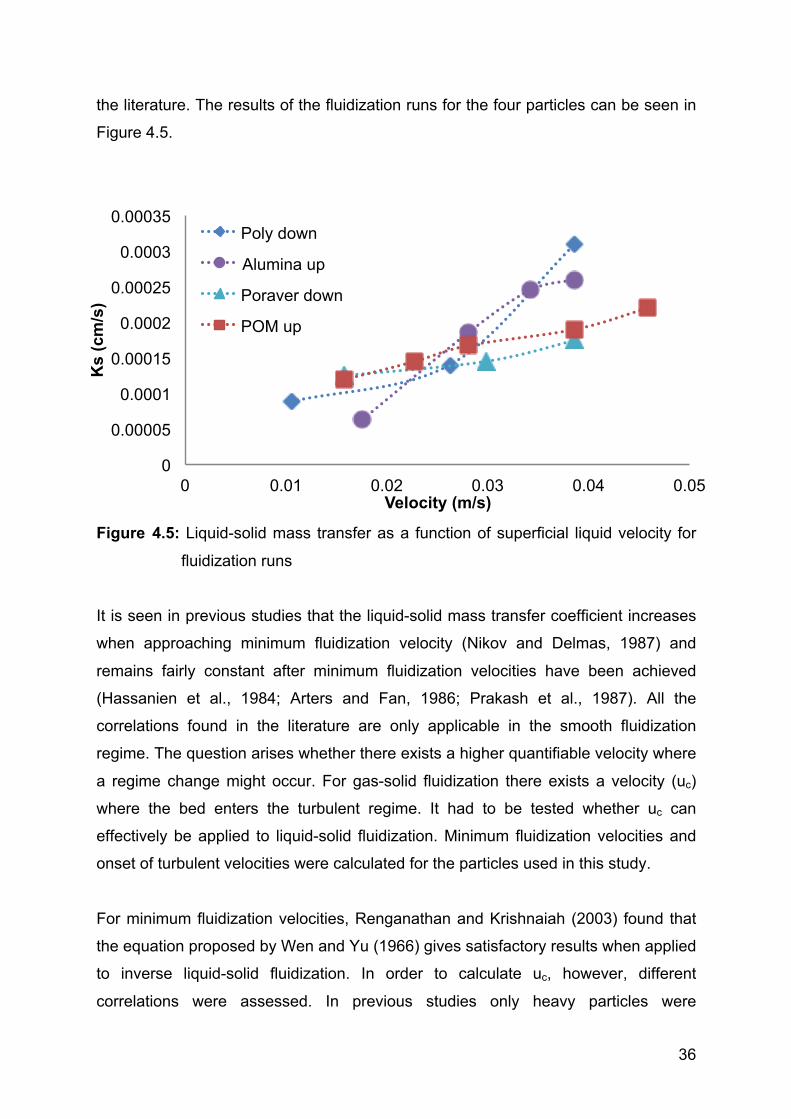
the literature. The results of the fluidization runs for the four particles can be seen in

Figure 4.5.

Figure 4.5: Liquid-solid mass transfer as a function of superficial liquid velocity for

fluidization runs

It is seen in previous studies that the liquid-solid mass transfer coefficient increases

when approaching minimum fluidization velocity (Nikov and Delmas, 1987) and

remains fairly constant after minimum fluidization velocities have been achieved

(Hassanien et al., 1984; Arters and Fan, 1986; Prakash et al., 1987). All the

correlations found in the literature are only applicable in the smooth fluidization

regime. The question arises whether there exists a higher quantifiable velocity where

a regime change might occur. For gas-solid fluidization there exists a velocity (uc)

where the bed enters the turbulent regime. It had to be tested whether uc can

effectively be applied to liquid-solid fluidization. Minimum fluidization velocities and

onset of turbulent velocities were calculated for the particles used in this study.

For minimum fluidization velocities, Renganathan and Krishnaiah (2003) found that

the equation proposed by Wen and Yu (1966) gives satisfactory results when applied

to inverse liquid-solid fluidization. In order to calculate uc, however, different

correlations were assessed. In previous studies only heavy particles were

0

0.00005

0.0001

0.00015

0.0002

0.00025

0.0003

0.00035

0 0.01 0.02 0.03 0.04 0.05

Ks

(cm

/s)

Velocity (m/s)

Poly down

Alumina up

Poraver down

POM up

37

investigated and therefore the turbulent regime was difficult to attain and was not

investigated for liquid-solid fluidization. Correlations found in the literature are based

on gas-solid systems (with some liquid-solid data) and were tested to see if they

predict proper uc values for the data obtained in this study. The correlation proposed

by Nakajima et al. (1991) was used for Poraver, POM and polypropylene because it

can be used for a very wide variety of particles. Their correlation can be seen in

Equation (4.1):

!"! = 0.633!"!.!"# (4.1)

The correlation proposed by Lee and Kim (1990) was chosen for alumina because

their study was done with glass beads with similar physical characteristics to those of

alumina. The authors, however, used air as their fluidization medium. Their

correlation can be seen in Equation 4.2:

!"! = 0.7!"!.!"# (4.2)

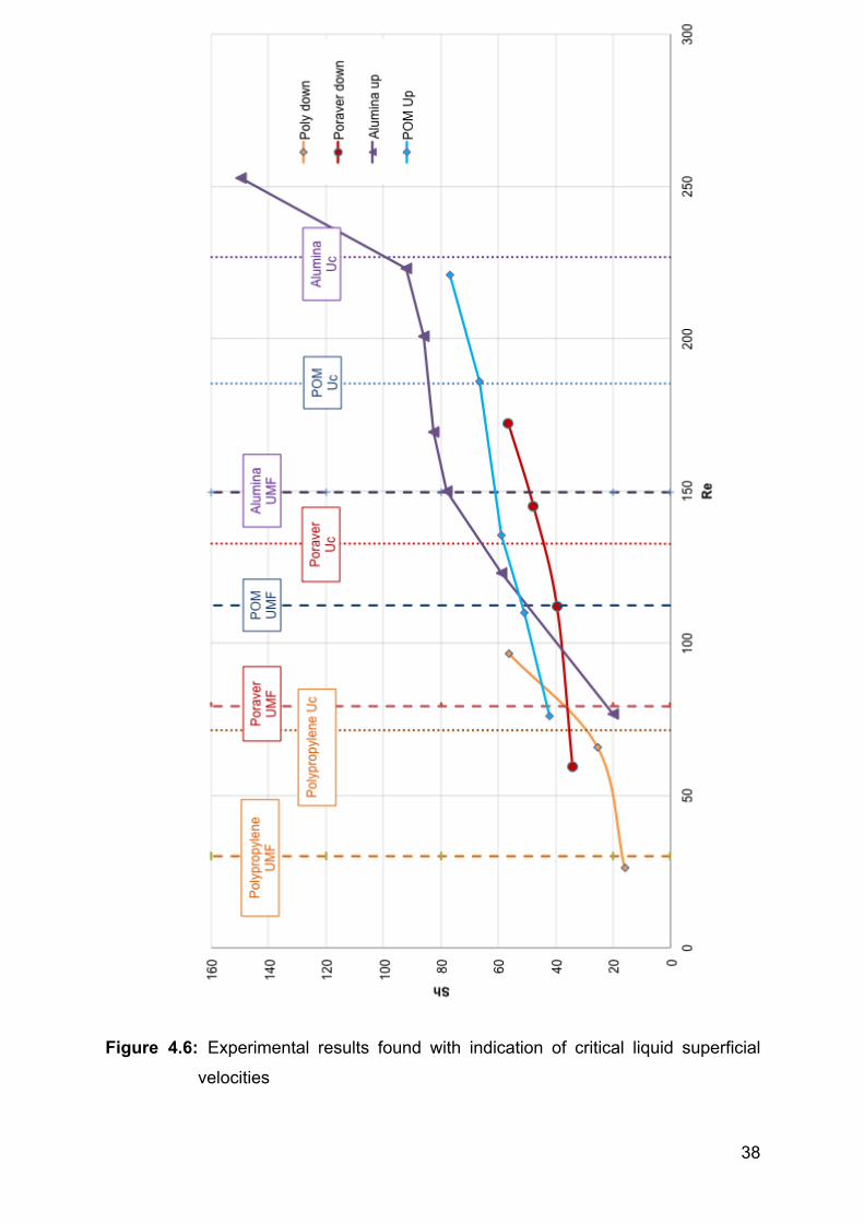
From these Rec values the onset of turbulence velocities (uc) can be determined.

When these flow regimes were added to the experimental data different trends were

identified with more ease, as seen in Figure 4.6. Nikov and Delmas (1987) also

found that the mass transfer rate increases near minimum fluidization velocities as

seen for alumina and POM particles. Hassanien et al. (1984), Arters and Fan (1986)

and Prakash et al. (1987) all found that when the minimum fluidization velocity is

reached the mass transfer stays fairly unchanged. This trend can be seen in Figure

4.6 for all four particles tested.

38

Figure 4.6: Experimental results found with indication of critical liquid superficial

velocities

!

39

It can be seen in Figure 4.6 that the Sh number increases with an increase in Re for

all four particles. It is also seen that higher Sh values are possible for particles with

higher minimum fluidization velocities. The liquid-solid mass transfer increases until

umf is reached. For particles with higher umf values, higher mass transfer coefficients

are possible. When the liquid velocity exceeds that of uc a slight increase in mass

transfer coefficients was seen for POM and Poraver, whereas for PP and alumina a

greater increase was seen. The greater increase for alumina can be due to the fact

that alumina particles are very heavy and with increased liquid velocities the

collisions between the particles may have caused some coated benzoic acid to be

chipped off the particles. Polypropylene has the smallest density difference and

therefore at very high liquid velocities the particle bed expanded the full length of the

reactor causing collisions between the particles and the liquid distributor. No decisive

conclusions can be reached on this increase after uc because it only occurs for two

of the four particles. Table 4.2 shows the density differences between the four

particles and water along with the Reynolds number at minimum fluidization and uc.

This gives an indication where the umf – uc window is reached.

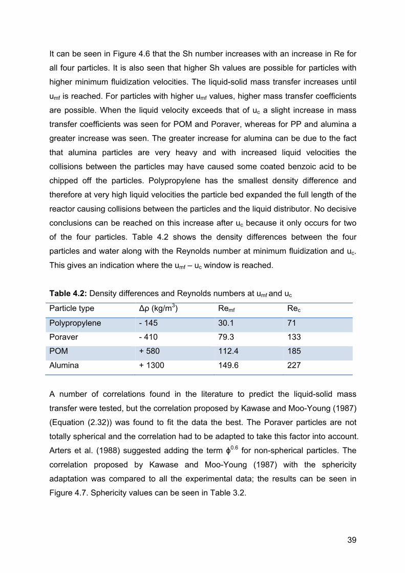
Table 4.2: Density differences and Reynolds numbers at umf and uc

Particle type Δρ (kg/m3) Remf Rec

Polypropylene - 145 30.1 71

Poraver - 410 79.3 133

POM + 580 112.4 185

Alumina + 1300 149.6 227

A number of correlations found in the literature to predict the liquid-solid mass

transfer were tested, but the correlation proposed by Kawase and Moo-Young (1987)

(Equation (2.32)) was found to fit the data the best. The Poraver particles are not

totally spherical and the correlation had to be adapted to take this factor into account.

Arters et al. (1988) suggested adding the term ϕ0.6 for non-spherical particles. The

correlation proposed by Kawase and Moo-Young (1987) with the sphericity

adaptation was compared to all the experimental data; the results can be seen in

Figure 4.7. Sphericity values can be seen in Table 3.2.

40

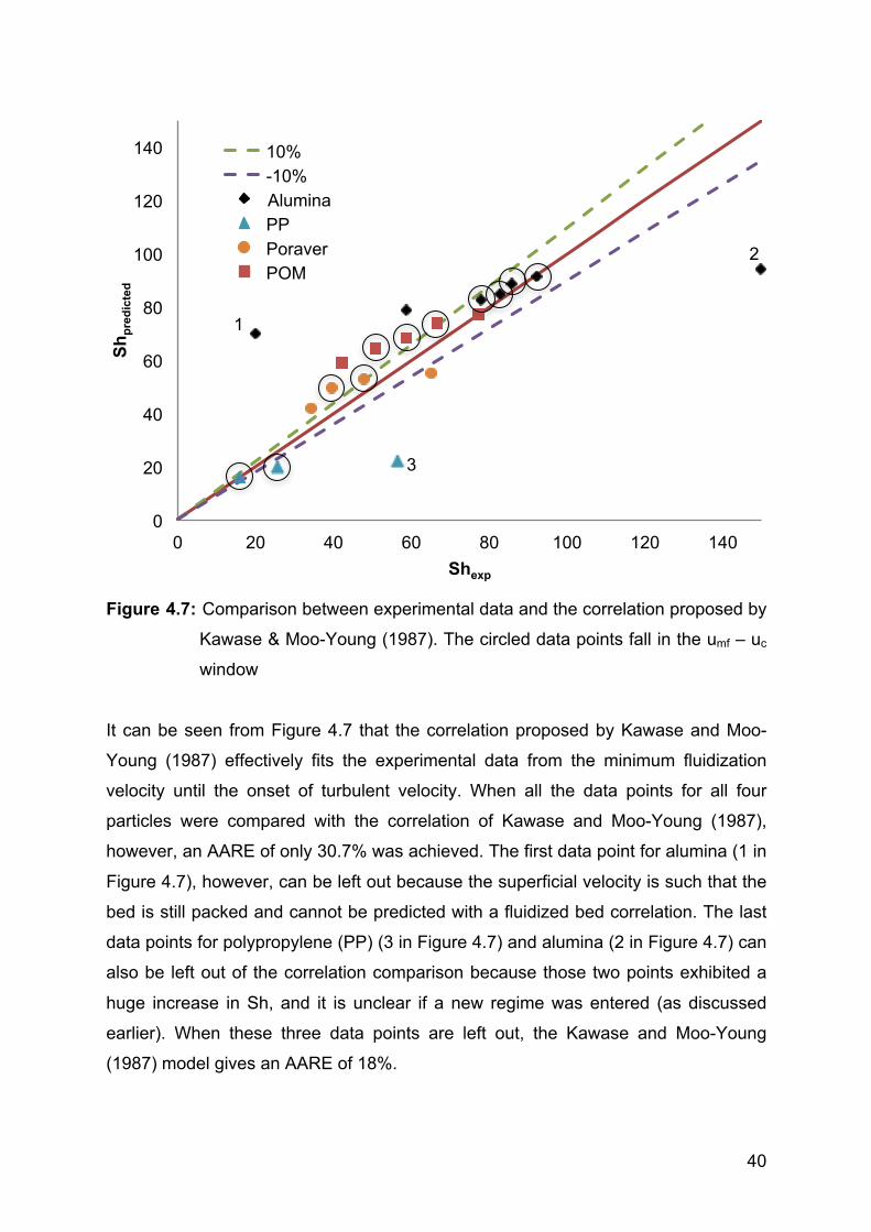
Figure 4.7: Comparison between experimental data and the correlation proposed by

Kawase & Moo-Young (1987). The circled data points fall in the umf – uc

window

It can be seen from Figure 4.7 that the correlation proposed by Kawase and Moo-

Young (1987) effectively fits the experimental data from the minimum fluidization

velocity until the onset of turbulent velocity. When all the data points for all four

particles were compared with the correlation of Kawase and Moo-Young (1987),

however, an AARE of only 30.7% was achieved. The first data point for alumina (1 in

Figure 4.7), however, can be left out because the superficial velocity is such that the

bed is still packed and cannot be predicted with a fluidized bed correlation. The last

data points for polypropylene (PP) (3 in Figure 4.7) and alumina (2 in Figure 4.7) can

also be left out of the correlation comparison because those two points exhibited a

huge increase in Sh, and it is unclear if a new regime was entered (as discussed

earlier). When these three data points are left out, the Kawase and Moo-Young

(1987) model gives an AARE of 18%.

0

20

40

60

80

100

120

140

0 20 40 60 80 100 120 140

Sh p

redi

cted

Shexp

10% -10% Alumina PP Poraver POM

2

3

1

41

The correlation proposed by Kawase & Moo-Young (1987) can be seen below:

!ℎ =  0.162(!!!!

!!)!.!"!"!/! (2.32)

The minimum fluidization velocity plays a big role and therefore a new model was

correlated that includes the particle characteristics in the form of the dimensionless

group, the Archimedes number. The correlation proposed can be seen in Equation

(4.3).

!ℎ = 0.05!"!.!"!"!.!! !" !.!" (4.3)

The addition of the Archimedes number makes for a more universal and robust

correlation. Adding the particle characteristics to the correlation makes the

correlation more mechanically sound. The values for the constants were determined

by comparing the correlation to the experimental results and minimizing the AARE

The absolute value of the Archimedes number needs to be taken into account

because some of the particles have lower densities than that of water and therefore

yield a negative Archimedes number. Equation (4.3) gave an AARE of 8% when

compared to the experimental results (excluding the three previously mentioned data

points), which is an improvement on the correlations found in the literature. This

correlation can be used for different particle densities up to the onset of turbulent

regime velocity (uc). Figure 4.8 shows how the new correlation compares to the

experimentally determined Sh numbers (Shexp).

42

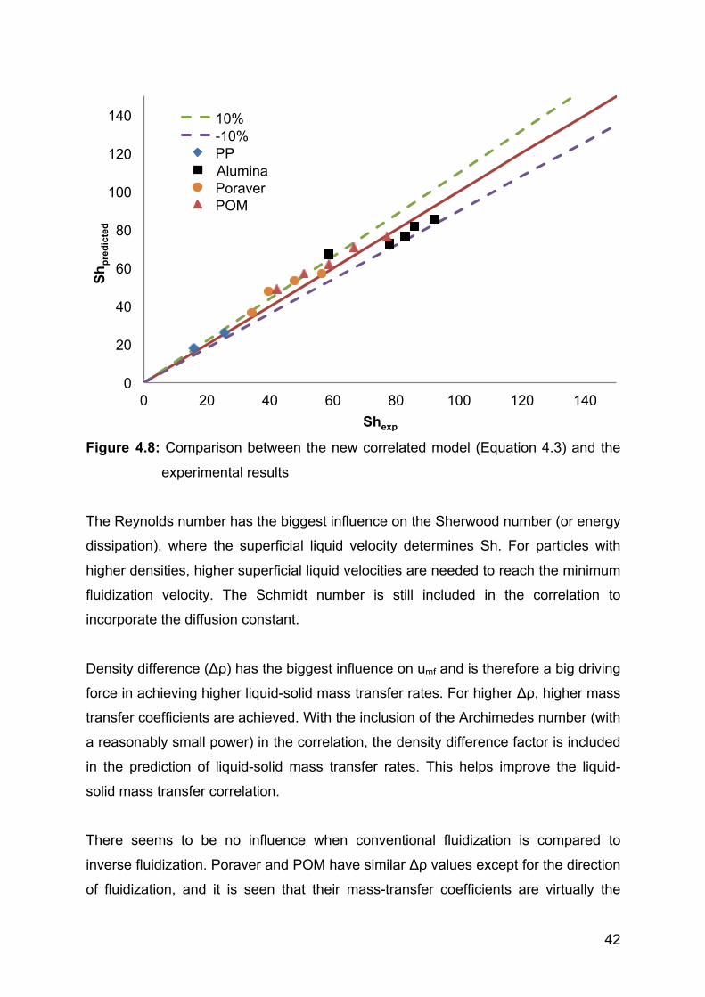
Figure 4.8: Comparison between the new correlated model (Equation 4.3) and the

experimental results

The Reynolds number has the biggest influence on the Sherwood number (or energy

dissipation), where the superficial liquid velocity determines Sh. For particles with

higher densities, higher superficial liquid velocities are needed to reach the minimum

fluidization velocity. The Schmidt number is still included in the correlation to

incorporate the diffusion constant.

Density difference (Δρ) has the biggest influence on umf and is therefore a big driving

force in achieving higher liquid-solid mass transfer rates. For higher Δρ, higher mass

transfer coefficients are achieved. With the inclusion of the Archimedes number (with

a reasonably small power) in the correlation, the density difference factor is included

in the prediction of liquid-solid mass transfer rates. This helps improve the liquid-

solid mass transfer correlation.

There seems to be no influence when conventional fluidization is compared to

inverse fluidization. Poraver and POM have similar Δρ values except for the direction

of fluidization, and it is seen that their mass-transfer coefficients are virtually the

0

20

40

60

80

100

120

140

0 20 40 60 80 100 120 140

Sh p

redi

cted

Shexp

10% -10% PP Alumina Poraver POM

43

same. POM only slightly outperforms Poraver because its Δρ is slightly higher. It can

be concluded from the presented results that the direction of liquid flow has no

influence on liquid-solid mass transfer for two-phase fluidized beds.

4.2.2 Packed bed

All four particle types can also be run in a packed bed mode. For the alumina and

POM particles the reactor was run in a down-flow manner while for the Poraver and

polypropylene particles the reactor was run in an up-flow manner. Similar dissolution

trends were found to the ones shown in the previous section, and liquid-solid mass

transfer coefficients were determined from those trends.

These data were compared to one of the correlations found in the literature to see

how it compares to previous studies. The most extensively used model in the

literature is the one by Thoenes and Kramers (1958). The authors tested eight

different particles in a packed bed manner and compiled a model to fit these data

and those of previous studies. They correlated different complex correlations but

found that the correlation seen in Equation (4.4) gave a deviation of only ±10% for all

438 mass transfer rates. This correlation was compared to the data obtained.

Figure 4.9 shows the data for two of the particle types used compared to the

Thoenes and Kramers (1958) model.

!ℎ′ = 1.0  (!"′)!!!"

!! (4.4)

Sh’  and Re’ are defined in Equations (4.5) and (4.6), where Φ is the void fraction

of the packed bed and γ is the external shape factor.

!ℎ′ = !!Φ(!!Φ)!

(4.5)

!"′ = !"Φ(!!Φ)!

(4.6)

44

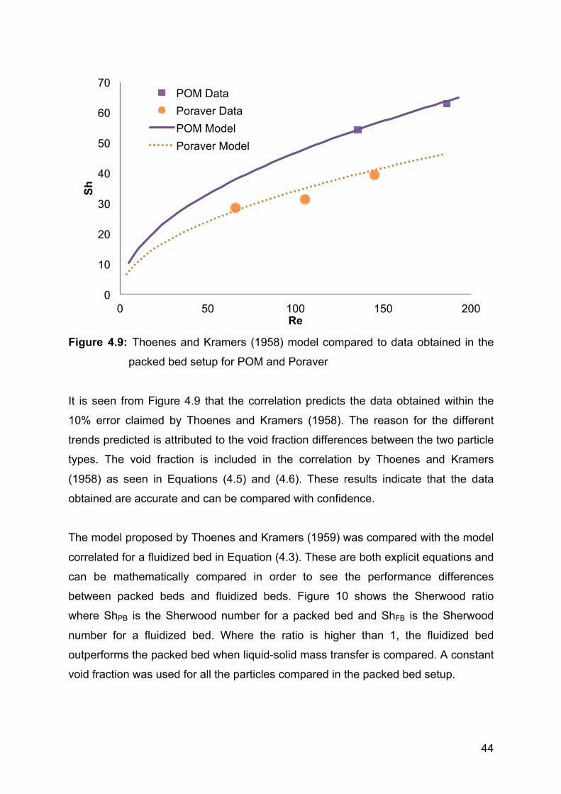
Figure 4.9: Thoenes and Kramers (1958) model compared to data obtained in the

packed bed setup for POM and Poraver

It is seen from Figure 4.9 that the correlation predicts the data obtained within the

10% error claimed by Thoenes and Kramers (1958). The reason for the different

trends predicted is attributed to the void fraction differences between the two particle

types. The void fraction is included in the correlation by Thoenes and Kramers

(1958) as seen in Equations (4.5) and (4.6). These results indicate that the data

obtained are accurate and can be compared with confidence.

The model proposed by Thoenes and Kramers (1959) was compared with the model

correlated for a fluidized bed in Equation (4.3). These are both explicit equations and

can be mathematically compared in order to see the performance differences

between packed beds and fluidized beds. Figure 10 shows the Sherwood ratio

where ShPB is the Sherwood number for a packed bed and ShFB is the Sherwood

number for a fluidized bed. Where the ratio is higher than 1, the fluidized bed

outperforms the packed bed when liquid-solid mass transfer is compared. A constant

void fraction was used for all the particles compared in the packed bed setup.

0

10

20

30

40

50

60

70

0 50 100 150 200

Sh

Re

POM Data Poraver Data POM Model Poraver Model

45

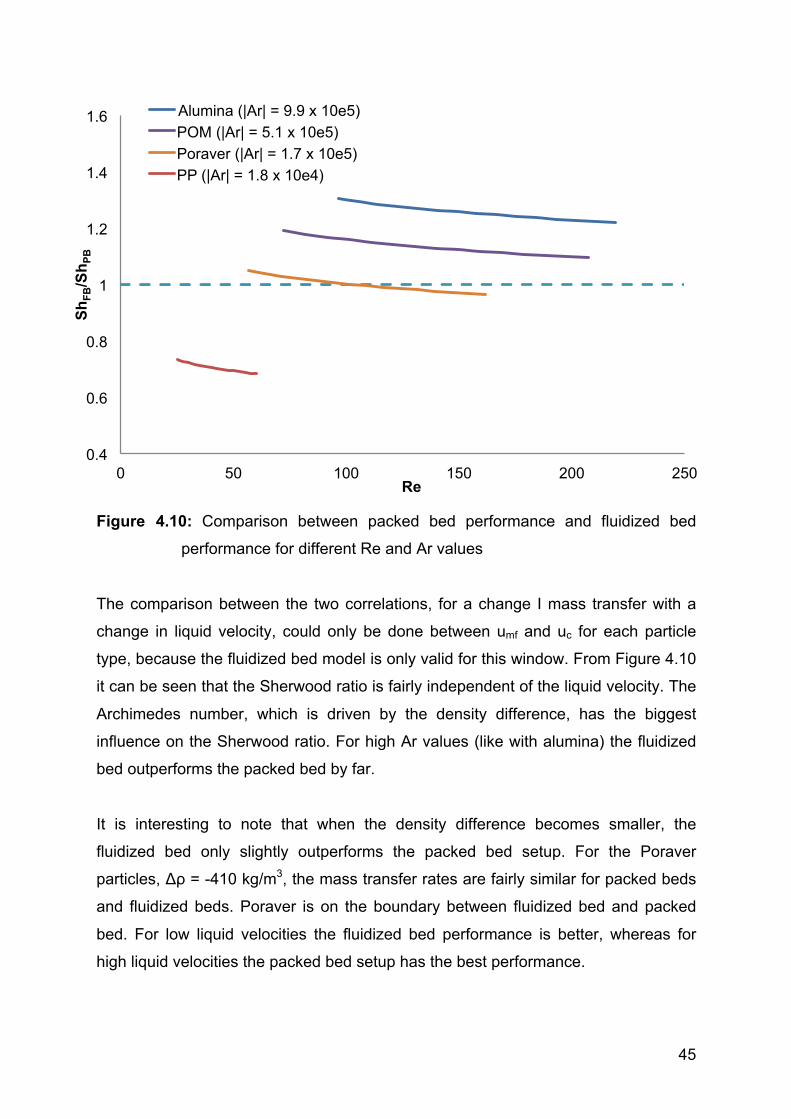
Figure 4.10: Comparison between packed bed performance and fluidized bed

performance for different Re and Ar values

The comparison between the two correlations, for a change I mass transfer with a

change in liquid velocity, could only be done between umf and uc for each particle

type, because the fluidized bed model is only valid for this window. From Figure 4.10

it can be seen that the Sherwood ratio is fairly independent of the liquid velocity. The

Archimedes number, which is driven by the density difference, has the biggest

influence on the Sherwood ratio. For high Ar values (like with alumina) the fluidized

bed outperforms the packed bed by far.

It is interesting to note that when the density difference becomes smaller, the

fluidized bed only slightly outperforms the packed bed setup. For the Poraver

particles, Δρ = -410 kg/m3, the mass transfer rates are fairly similar for packed beds

and fluidized beds. Poraver is on the boundary between fluidized bed and packed

bed. For low liquid velocities the fluidized bed performance is better, whereas for

high liquid velocities the packed bed setup has the best performance.

0.4

0.6

0.8

1

1.2

1.4

1.6

0 50 100 150 200 250

ShFB

/Sh P

B

Re

Alumina (|Ar| = 9.9 x 10e5) POM (|Ar| = 5.1 x 10e5) Poraver (|Ar| = 1.7 x 10e5) PP (|Ar| = 1.8 x 10e4)

46

From the Polypropylene runs it can be seen that the liquid-solid mass transfer for the

packed beds is better than for the fluidized beds. The very small density difference

(Δρ = -145 kg/m3) influences the liquid-solid mass transfer to the extent that the

packed bed substantially outperforms the fluidized bed.

4.3 Three phase fluidization

In order to investigate the influence of three-phase fluidization on the liquid-solid

mass transfer, gas was introduced at the bottom of the reactor co-current to the

liquid flow. For three phase fluidization only up-flow could be compared because

counter-current flow with liquid down-flow creates a pressure differential over the top

liquid distributer that complicates operation. For this reason only the two higher-

density particle types, POM and alumina, were tested in three-phase (up-flow)

fluidization. For future development a different reactor design will be needed in order

to eliminate the differential pressure. A reactor is needed where the liquid can be

introduced at the side of the reactor with a gas-settling zone at the top.

A number of runs were done at different liquid velocities. A constant gas vvm

(volume of gas fed to the reactor per volume of the reactor) of 162 ml/ml.min was fed

to the reactor for all runs. The results obtained for alumina particles can be seen in

Figure 4.11. The minimum fluidization velocities can be determined using the

correlations in Section 1.4.

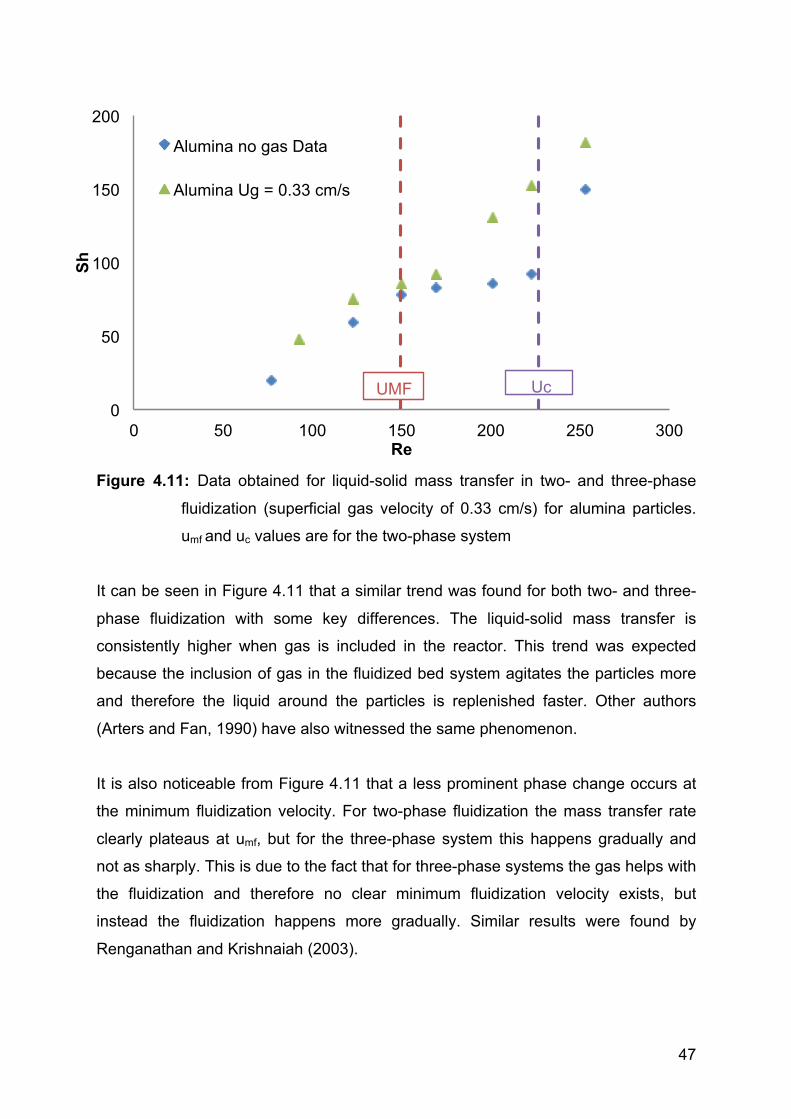
47

Figure 4.11: Data obtained for liquid-solid mass transfer in two- and three-phase

fluidization (superficial gas velocity of 0.33 cm/s) for alumina particles.

umf and uc values are for the two-phase system

It can be seen in Figure 4.11 that a similar trend was found for both two- and three-

phase fluidization with some key differences. The liquid-solid mass transfer is

consistently higher when gas is included in the reactor. This trend was expected

because the inclusion of gas in the fluidized bed system agitates the particles more

and therefore the liquid around the particles is replenished faster. Other authors

(Arters and Fan, 1990) have also witnessed the same phenomenon.

It is also noticeable from Figure 4.11 that a less prominent phase change occurs at

the minimum fluidization velocity. For two-phase fluidization the mass transfer rate

clearly plateaus at umf, but for the three-phase system this happens gradually and

not as sharply. This is due to the fact that for three-phase systems the gas helps with

the fluidization and therefore no clear minimum fluidization velocity exists, but

instead the fluidization happens more gradually. Similar results were found by

Renganathan and Krishnaiah (2003).

0

50

100

150

200

0 50 100 150 200 250 300

Sh

Re

Alumina no gas Data

Alumina Ug = 0.33 cm/s

UMF Uc

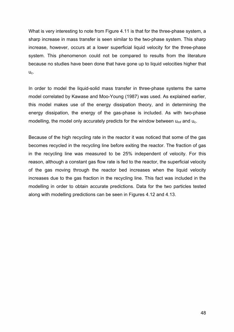
48

What is very interesting to note from Figure 4.11 is that for the three-phase system, a

sharp increase in mass transfer is seen similar to the two-phase system. This sharp

increase, however, occurs at a lower superficial liquid velocity for the three-phase

system. This phenomenon could not be compared to results from the literature

because no studies have been done that have gone up to liquid velocities higher that

uc.

In order to model the liquid-solid mass transfer in three-phase systems the same

model correlated by Kawase and Moo-Young (1987) was used. As explained earlier,

this model makes use of the energy dissipation theory, and in determining the

energy dissipation, the energy of the gas-phase is included. As with two-phase

modelling, the model only accurately predicts for the window between umf and uc.

Because of the high recycling rate in the reactor it was noticed that some of the gas

becomes recycled in the recycling line before exiting the reactor. The fraction of gas

in the recycling line was measured to be 25% independent of velocity. For this

reason, although a constant gas flow rate is fed to the reactor, the superficial velocity

of the gas moving through the reactor bed increases when the liquid velocity

increases due to the gas fraction in the recycling line. This fact was included in the

modelling in order to obtain accurate predictions. Data for the two particles tested

along with modelling predictions can be seen in Figures 4.12 and 4.13.

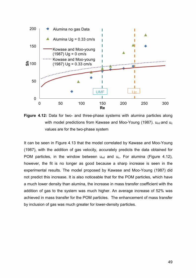
49

Figure 4.12: Data for two- and three-phase systems with alumina particles along

with model predictions from Kawase and Moo-Young (1987). umf and uc

values are for the two-phase system

It can be seen in Figure 4.13 that the model correlated by Kawase and Moo-Young

(1987), with the addition of gas velocity, accurately predicts the data obtained for

POM particles, in the window between umf and uc. For alumina (Figure 4.12),

however, the fit is no longer as good because a sharp increase is seen in the

experimental results. The model proposed by Kawase and Moo-Young (1987) did

not predict this increase. It is also noticeable that for the POM particles, which have

a much lower density than alumina, the increase in mass transfer coefficient with the

addition of gas to the system was much higher. An average increase of 52% was

achieved in mass transfer for the POM particles. The enhancement of mass transfer

by inclusion of gas was much greater for lower-density particles.

0

50

100

150

200

0 50 100 150 200 250 300

Sh

Re

Alumina no gas Data

Alumina Ug = 0.33 cm/s

Kowase and Moo-young (1987) Ug = 0 cm/s Kowase and Moo-young (1987) Ug = 0.33 cm/s

UMF Uc

50

Figure 4.13: Data for two- and three-phase systems with POM particles along with

model predictions by Kawase and Moo-Young (1987). umf and uc values

are for the two-phase system

20

40

60

80

100

120

0 50 100 150 200 250

Sh

Re

POM no gas

POM Ug = 0.33 cm/s

Kowase & Moo-Young (1987) Ug=0 cm/s Kowase & Moo-Young (1987) Ug=0.33 cm/s

UMF Uc

51

5. Conclusions

The liquid-solid mass transfer coefficient was experimentally determined in a novel

reactor, with external recycling. Liquid-solid experiments were performed in both up-

and down-flow mode depending on the particle density. In addition, three-phase

experiments were performed in concurrent up-flow mode. The dissolution of benzoic

acid method was adapted and used in order to quantify the liquid-solid mass transfer

rate. A broader understanding was reached with regard to a number of factors

influencing the liquid-solid mass transfer in a reactor and is discussed here.

The liquid-solid mass transfer increased until umf was reached, after which the

increase in mass transfer became slight. This was confirmed to be the minimum

fluidization regime. For two of the particles tested (alumina and polypropylene) there

exists a liquid velocity (uc) after which the mass transfer increases sharply. This was

deemed the transition to the turbulent regime as seen with gas-solid fluidization;

standard uc correlations were employed to determine this critical velocity for all the

particle types. After uc was reached only a slight increase in mass transfer

coefficients was seen for POM and Poraver. No decisive conclusions can be

reached on this increase after uc because it only occurs in two of the four particles.

It was found that the correlation proposed by Kawase and Moo-Young (1987) fits the

experimental data from the minimum fluidization velocity (umf) until the onset of

turbulent velocity (uc) with an AARE of 18%. A new correlation was proposed with

the inclusion of the dimensionless group, the Archimedes number. The correlation

proposed achieved an AARE of only 8% and can be seen in Equation (5.1).

!ℎ = 0.05!"!.!"!"!.!!!"!.!" (5.1)

When flow direction in a two-phase fluidized bed was compared, no significant

difference was found at similar liquid velocities in liquid-solid mass transfer if the

density difference (Δρ) between solid and liquid phases is the same. It can be

concluded that the direction of liquid flow has no influence on liquid-solid mass

transfer for two-phase fluidized beds. It was, however, found that density difference

52

(Δρ) has a significant influence on the liquid-solid mass transfer. For a higher Δρ,

higher mass transfer coefficients were achieved mainly because of the higher Re

numbers required to achieve fluidization.

The experimental results obtained for packed bed liquid-solid mass transfer

compared well with the model proposed by Thoenes and Kramers (1959). A

comparison between fluidized bed and packed bed liquid-solid mass transfer showed

that the Archimedes number (driven by density difference) had a major influence.

When Δρ is high, as for the alumina particles (Δρ = 1300 kg/m3), the fluidized bed

outperforms the packed bed (ShFB/ShPB = 1.25). When the density difference

becomes smaller, Δρ = 580 kg/m3, the fluidized bed only slightly outperforms the

packed bed setup. For a very small density difference (Δρ = -145 kg/m3) the packed

bed substantially outperforms the fluidized bed (ShFB/ShPB = 0.7). It was also noted

that the Sherwood ratio was not significantly dependent on the liquid velocity.

When liquid-solid mass transfer rates were determined for three-phase systems only

up-flow could be compared. The introduction of gas improves the liquid-solid mass

transfer at the same liquid velocity when two-phase and three-phase systems are

compared. It was also found that no significant transitions were seen between the

flow regimes as seen with two-phase fluidization. This was because a gradual

fluidization occurred with three-phase fluidization and not instantaneous fluidization

as with liquid-solid fluidized beds. The enhancement of mass transfer by inclusion of

gas was more severe for lower-density particles.

53

6. References

Arters, D. C. and Fan, L.S. (1986) “Solid-liquid mass transfer in a gas-liquid-solid

fluidized bed” Chemical Engineering Science, 41, 107-115.

Arters, D.C. and Fan, L (1990) “Experimental methods and correlation of solid-liquid

mass transfer in fluidized beds” Chemical Engineering Science, 45, 965-975.

Asai, A., Konishi, Y. and Maeda, H. (1985) Chem Eng Sci 40, 1573.

Banerjee, J. Basu, J.K. and Ganguly, U.P. (1999) “Some studies on the

hydrodynamics of reverse fluidization velocities”, Ind. Chem. Eng. 41 (1) 35–38.

Behkish, A., Lemoine, R., Oukaci, R. and Morsi, B.I. (2006) “Novel correlations for

gas holdup in large-scale slurry bubble column reactors operating under

elevated pressures and temperatures”, Chem. Eng. J., 115, 157–171.

Biswas, S.K. and Ganguly, U.P. (1997) “A preliminary study on the voidage–velocity

relationship in reverse fluidization”, Ind. Chem. Eng., 39, 303–306.

Buffière, P and Moletta, R. (1999) “Some hydrodynamic characteristics of inverse

three phase fluidized-bed reactors”, Chem. Eng. Sci., 54, 1233–1242.

Calderon, D.G., Buffiere, P., Moletta, R. and Elmaleh, S. (1998) “Anaerobic

digestion of wine distillery wastewater in down-flow fluidized bed”, Wat. Res. 32,

3593–3600.

Cho, Y.J., Park, H.Y., Kim, S.W., Kang, Y. and Kim, S.D.(2002) “Heat transfer and

hydrodynamics in two- and three-phase inverse fluidized beds” Ind. Eng. Chem.

Res., 41, 2058–2063.

Deckwer, W.D. (1980) Chem Eng Sci 35, 1341.

Delgado, J. M. P. Q. (2006) “Experimental data of solubility at different temperatures:

a simple technique”, Springer-Verlag.

Fan, L, Muroyama, K and Chern, S (1982) “Hydrodynamic characteristics of inverse

fluidization in liquid-solid and gas-liquid-solid systems”, Chemical Engineering

Journal, 24, 143-150.

54

Fan, L.S., (1989) “Gas–liquid–solid fluidization engineering”, Butterworths, Stoneham.

Fogler, H. S., (2009) “Elements of chemical reaction engineering”, prentice-hall,

englewood cliffs, New Jersey.

Fukuma, M., Sato, M., Muroyama, K. and Yasunishi, A., (1988) “Particle-to-liquid

mass transfer in gas-liquid-solid fluidization”, J. Chem. Engng Japan, 21, 231-

237.

Gamson B. W., (1951) “Heat and mass transfer (liquid solid systems)”. Chem. Engng

Prog, 47, 19-28.

Hassanien, S., Delmas, H. and Riba, J. P. (1984) “Transfert de matière liquid”,

Particules Entropie, 119, 17-26.

Ibrahim, Y. A. A., Briens, C. L., Margaritis, A. and Bergongnou, M. A. (1996)

“Hydrodynamic characteristics of a 3-phase inverse fluidized bed column”,

AIChE Journal, 42, 1889–1900.

Kawase, Y. and Moo-Young, M. (1987) “Solid-turbulent fluid heat and mass transfer:

a unified model based on the energy dissipation rate concept”, Chem. Engng J.

36,3140.

Khan, A.R. and Richardson, J.F. (1990) “Pressure gradient and friction factor for

sedimentation and fluidization of uniform spheres in liquids”, Chemical

Engineering Science, 45, 255–265.

Kikuchi, K., Suaawara. T. and Ohashi. H. (1983) “Correlation of mass transfer

coefficient between particles and liquid in liquid fluidized beds”, J. Chem.

Engng Japan, 16, 426428.

Kim, S.D. and Kang, Y. (1997) “Heat and mass transfer in three-phase fluidized-bed

reactor - an overview”, Chemical Engineering Science, 52, 3639–3660.

Krishnaiah, K., Guru, S. and Sekar, V. (1993) “Hydrodynamic studies on inverse

gas–liquid–solid fluidization”, Chemical Engineering Journal, 51, 109–112.

Kunii, D. and Levenspiel, O. (1999) Fluidization engineering, Butterworth-Heinemann,

London, Boston.

55

Lee, K. W. and Kim, J. C. (1990) “Experimental study of particle collection by small

cyclones”, Aerosol Science and Technology, 12, 1005 -1015.

Legile, P., Menard, G., Laurent, C., Thomas, D. and Bernis, A. (1992) “Contribution

to the study of an inverse 3-phase fluidized bed operating countercurrently”,

International Chemical Engineering, 32, 41–50.

Myre, D. and Macchi, A. (2010) “Heat transfer and bubble dynamics in a three-phase

inverse fluidized bed”, Chemical Engineering and Processing, 49, 523-529.

Nakajima, M., Harada, M., Asai, M., Yamazaki, R. and Jimbo, G. (1991) “Bubble

fraction and voidage in an emulsion phase in the transition to a turbulent

fluidized bed”, Circulating Fluidized Bed III (pp. 79-84). Oxford: Pergamon

Press.

Nikolov, L. and Karamanev, D. (1987) “Experimental study of the inverse fluidized

bed biofilm reactor”, Can. J. Chem. Eng., 65, 214–217.

Nikov, I. and Delmas, H. (1987) “Solid-liquid mass transfer in three-phase fixed and

fluidized beds”, Chemical Engineering Science, 42, 1089-1093.

Niven, R.K. (2002) “Physical insight into the Ergun and Wen & Yu equations for fluid

flow in packed and fluidized beds”, Chemical Engineering Science, 57, 527-534.

Prakash, A., Briens, C. L. and Bergougnou, M. A. (1987) “Mass transfer between

solid particles and liquid in a three phase fluidized bed”, Can. J. Chem. Eng, 65,

228-236.

Qing-Zhu, J., Pei-Sheng, M., Huan, Z., Shu-Qian, X., Qiang, W. and Yan, Q. (2006)

“The effect of temperature on the solubility of benzoic acid derivatives in water”,

College of Chemical Engineering, Tianjin University, Tianjin 300072, P.R.

China.

Renganathan, T. and Krishnaiah, K. (2003) “Prediction of minimum fluidization

velocity in two and three phase inverse fluidized beds”, Can. J. Chem. Eng., 81,

853–860.

Renganathan, T. and Krishnaiah, K. (2004) “Liquid phase mixing in 2-phase liquid-

solid inverse fluidized bed”, Chemical Engineering Journal, 98, 213-218.

56

Renganathan, T. and Krishnaiah, K. (2005) “Voidage characteristics and prediction

of bed expansion in liquid-solid inverse fluidized bed”, Chemical Engineering

Science, 60, 2545-2555.

Richardson, J. F. and Zaki, W. N. (1954) “Sedimentation and fluidization: Part I”,

Trans. Inst. Chem. Eng., 32, 3553.

Roy, S. and Dudukovic, M.P., (2001) “Flow mapping and modelling of liquid–solid

risers”, Industrial and Engineering Chemistry Research, 40, 5440–5454.

Sanger, P. and Deckwer, W.D. (1981) Chem Eng J, 22, 179.

Sano, Y.N., Yamaguchi, N. and Adachi, T. (1974) Chem Eng Jpn 1, 255.

Shen, G.C., Geankoplis, C.J. and Brodkey, R.S. (1985) “A note on particle-liquid

mass transfer in a fluidized bed of small irregular-shaped benzoic acid

particles”, Chemical Engineering Science, 40: 9, 1797-1802.

Son, S.M., Kang, S.H., Kim, U.Y., Kang, Y. and Kim, S.D. (2007) “Bubble properties

in three-phase inverse fluidized beds with viscous liquid medium”, Chem. Eng.

Process, 46, 736–741.

Thoenes, D. and Kramers, H. (1958) “Mass transfer from spheres in various regular

packings to a flowing fluid”, Chemical Engineering Science 8, 271-283.

Turton, R. and Clark, N.N. (1987) “An explicit relationship to predict spherical particle

velocity”, Powder Technology, 53, 127–129.

Ulaganathan, N. and Krishnaiah, K. (1996) “Hydrodynamic characteristics of two-

phase inverse fluidized bed”, Bioprocess Eng, 15:159–164.

Vijayalakshmi, A.C., Balamurugan, M, Sivakumar, M., Samuel, T.N. and Velan, M.

(2000) “Minimum fluidization velocity and friction factor in a liquid-solid inverse

fluidized bed reactor”, Bioprocess Biosys Eng, 22:461–466.

Wen, C.Y. and Yu, Y.H. (1966) “Mechanics of fluidization”, Chem. Eng. Prog.

Symposium Series, 66, 101–111.

Yang, X.L., Wild, G. and Euzen, J.P. (1993) “Study of liquid retention in fixed- bed

reactors with upward flow of gas and liquid”, Int. Chem. Eng. 33, 72–84.

57

Zhang, J.P., Epstein, N., Grace J.R. and Zhu, J. (1995) “Minimum liquid fluidization

velocity of gas–liquid fluidized beds”, Trans. IchemE. 73, 347–353.

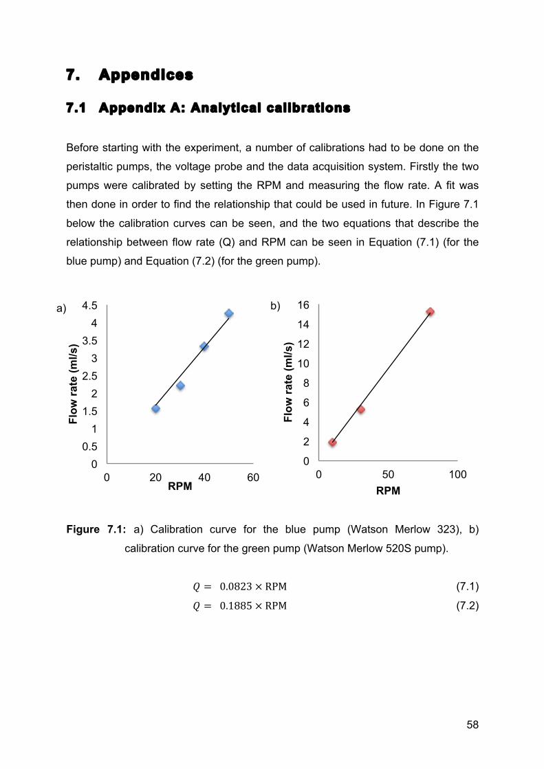
58

7. Appendices

7.1 Appendix A: Analytical calibrations

Before starting with the experiment, a number of calibrations had to be done on the

peristaltic pumps, the voltage probe and the data acquisition system. Firstly the two

pumps were calibrated by setting the RPM and measuring the flow rate. A fit was

then done in order to find the relationship that could be used in future. In Figure 7.1

below the calibration curves can be seen, and the two equations that describe the

relationship between flow rate (Q) and RPM can be seen in Equation (7.1) (for the

blue pump) and Equation (7.2) (for the green pump).

Figure 7.1: a) Calibration curve for the blue pump (Watson Merlow 323), b)

calibration curve for the green pump (Watson Merlow 520S pump).

! =    0.0823  ×  RPM (7.1)

! =    0.1885  ×  RPM (7.2)

0 0.5

1 1.5

2 2.5

3 3.5

4 4.5

0 20 40 60

Flow

rat

e (m

l/s)

RPM

a)

2

0

2

4

6

8

10

12

14

16

0 50 100

Flow

rat

e (m

l/s)

RPM

1

b)

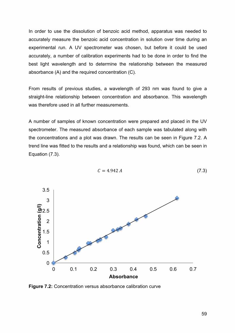
59

In order to use the dissolution of benzoic acid method, apparatus was needed to

accurately measure the benzoic acid concentration in solution over time during an

experimental run. A UV spectrometer was chosen, but before it could be used

accurately, a number of calibration experiments had to be done in order to find the

best light wavelength and to determine the relationship between the measured

absorbance (A) and the required concentration (C).

From results of previous studies, a wavelength of 293 nm was found to give a

straight-line relationship between concentration and absorbance. This wavelength

was therefore used in all further measurements.

A number of samples of known concentration were prepared and placed in the UV

spectrometer. The measured absorbance of each sample was tabulated along with

the concentrations and a plot was drawn. The results can be seen in Figure 7.2. A

trend line was fitted to the results and a relationship was found, which can be seen in

Equation (7.3).

! = 4.942  ! (7.3)

Figure 7.2: Concentration versus absorbance calibration curve

0

0.5

1

1.5

2

2.5

3

3.5

0 0.1 0.2 0.3 0.4 0.5 0.6 0.7

Con

cent

ratio

n (g

/l)

Absorbance

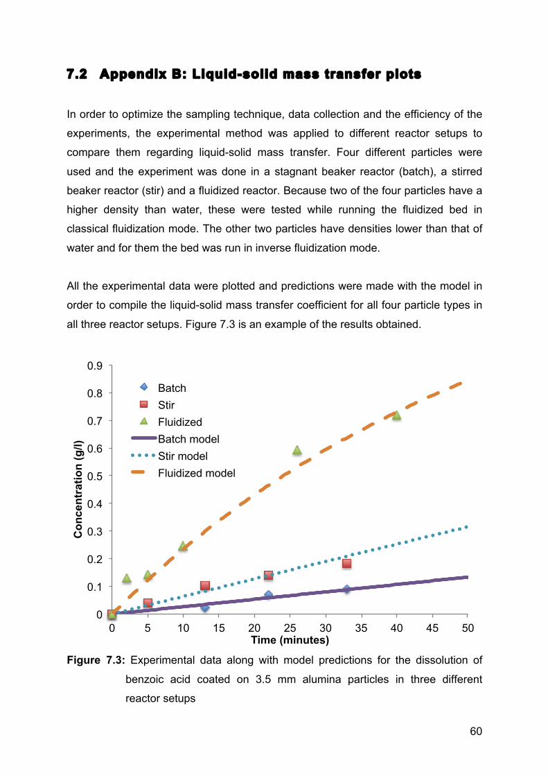
60

7.2 Appendix B: Liquid-solid mass transfer plots

In order to optimize the sampling technique, data collection and the efficiency of the

experiments, the experimental method was applied to different reactor setups to

compare them regarding liquid-solid mass transfer. Four different particles were

used and the experiment was done in a stagnant beaker reactor (batch), a stirred

beaker reactor (stir) and a fluidized reactor. Because two of the four particles have a

higher density than water, these were tested while running the fluidized bed in

classical fluidization mode. The other two particles have densities lower than that of

water and for them the bed was run in inverse fluidization mode.

All the experimental data were plotted and predictions were made with the model in

order to compile the liquid-solid mass transfer coefficient for all four particle types in

all three reactor setups. Figure 7.3 is an example of the results obtained.

Figure 7.3: Experimental data along with model predictions for the dissolution of

benzoic acid coated on 3.5 mm alumina particles in three different

reactor setups

0

0.1

0.2

0.3

0.4

0.5

0.6

0.7

0.8

0.9

0 5 10 15 20 25 30 35 40 45 50

Con

cent

ratio

n (g

/l)

Time (minutes)

Batch Stir Fluidized Batch model Stir model Fluidized model

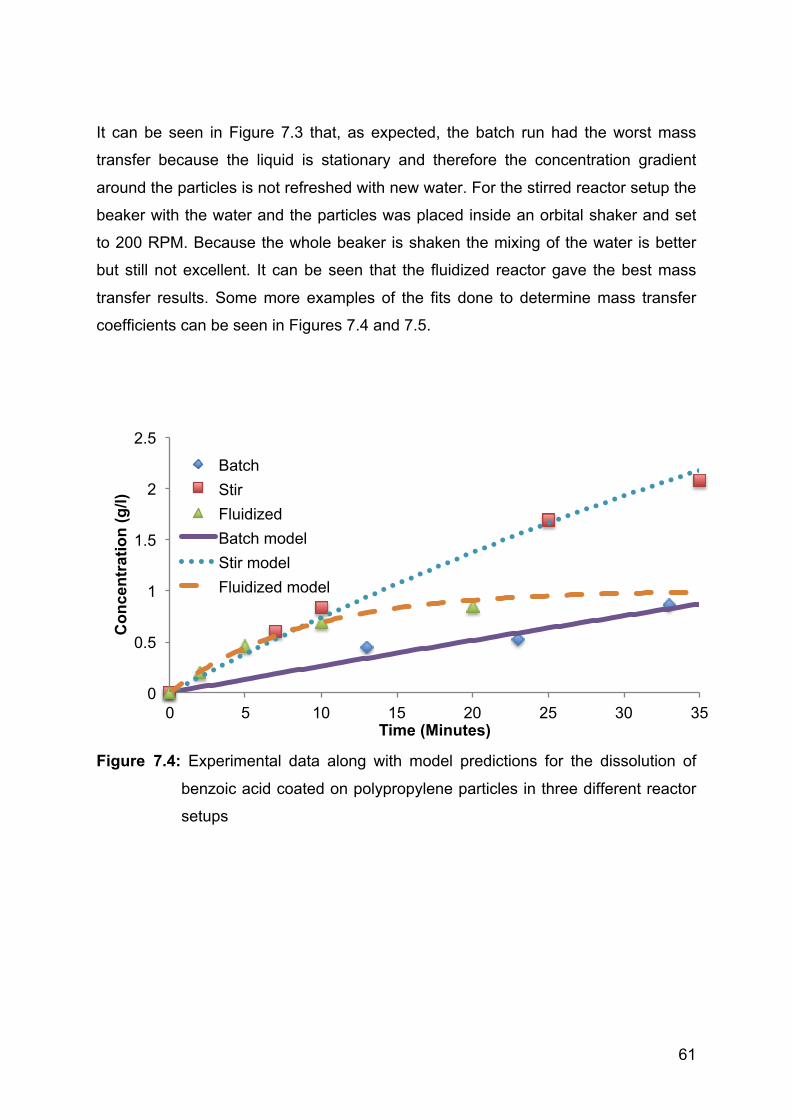
61

It can be seen in Figure 7.3 that, as expected, the batch run had the worst mass

transfer because the liquid is stationary and therefore the concentration gradient

around the particles is not refreshed with new water. For the stirred reactor setup the

beaker with the water and the particles was placed inside an orbital shaker and set

to 200 RPM. Because the whole beaker is shaken the mixing of the water is better

but still not excellent. It can be seen that the fluidized reactor gave the best mass

transfer results. Some more examples of the fits done to determine mass transfer

coefficients can be seen in Figures 7.4 and 7.5.

Figure 7.4: Experimental data along with model predictions for the dissolution of

benzoic acid coated on polypropylene particles in three different reactor

setups

0

0.5

1

1.5

2

2.5

0 5 10 15 20 25 30 35

Con

cent

ratio

n (g

/l)

Time (Minutes)

Batch Stir Fluidized Batch model Stir model Fluidized model

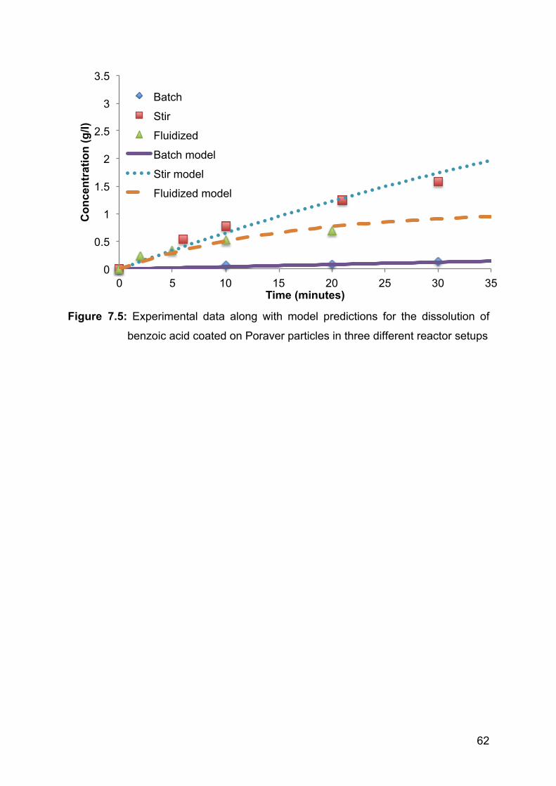
62

Figure 7.5: Experimental data along with model predictions for the dissolution of

benzoic acid coated on Poraver particles in three different reactor setups

0

0.5

1

1.5

2

2.5

3

3.5

0 5 10 15 20 25 30 35

Con

cent

ratio

n (g

/l)

Time (minutes)

Batch

Stir

Fluidized

Batch model

Stir model

Fluidized model

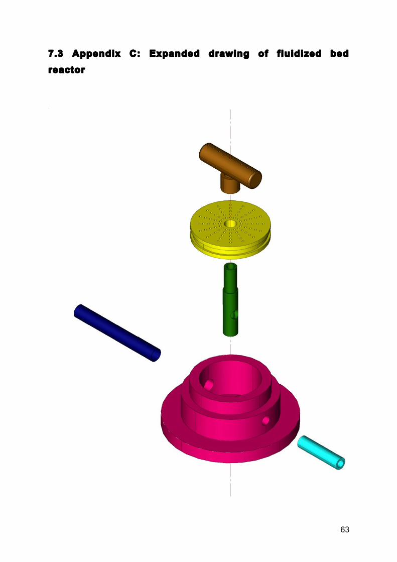
63

7.3 Appendix C: Expanded drawing of fluidized bed reactor