linking tiam and klem: economic impacts of wb2d mitigation pathways
TRANSCRIPT

Linking TIAM-KLEM: Economic impacts of WB2D mitigation pathways(Work in Progress, please don’t cite)
James Glynn, Frédéric Ghersi, Brian Ó Gallachóir
70th ETSAP Workshop
CIEMAT, MADRID | 17th – 18th November 2016

Outline
• What is the key motivation?• Understand feedbacks, structural changes and welfare effects
due to energy system decarbonisation
• Update on soft-link method between TIAM and KLEM• KLEM Computable General Model
• Harmonising updated World Bank/OECD Driver to TIAM
• Some precursory results, aggregated at world level highlighting the difference between BASE economic outlook and current macroeconomic outlook from SSP/OECD/World Banks

Why Hybrid Linking?
• Update TIAM Macroeconomic outlook(s)
• Harmonisation of energy service demands with changing economic outlook.
• Aim for best of both worlds.• Technological Explicitness• Macroeconomic realism• Sectoral Dynamics (Energy, Non Energy, Households)
• Demand response is considerable in decarbonisation scenarios.
• Moving forward from TIAM-MACRO/MSA• Investigate multi-sector dynamics
• Aim for better representation socio-economic dynamics

Overview of linkage
• TIMES-MACRO (Remme & Blesl, 2006)
• TIAM-KLEM
TIAM
Sectoral
Energy p&qs
KLEM
Labour
ES investment
Households’ consumption
Public consumption
International trade
Investment
Non-E/E Capital
Non-E output
?Non-E prices?

KLEM Prerequisites
• National accounting framework to access• Complete cost structures K, L, E, M(1,…,n)
• Inter-industry flows i.e. structural change, dematerialisation
• Market instruments recycling options
• Distributive issues, at least firms/government/households
• Dual accounting in monetary and physical units• To keep track of energy volumes in stand-alone versions
• To model agent-specific pricing
• Explicit investment profiles• To account for transitional strain on shorter time intervals
KLEM at a glimpse
• CGEM with 2 primary factors L and K, 1 E good, 1 non-Egood
• Recursive dynamics driven by• Exogenous L supply and productivity (SSP)
• K accumulation via exogenous investment & depreciation rates
• Public expenses constant share of GDP, constant (rough) tax system
• Operates on hybrid energy/economy matrix obtained from crossing GTAP and TIAM data
6/16

B$ Non-E E C G I X Uses
Non-E 14 085 90 9 022 3 235 3 410 2 158 32 000
E 430 627 249 - - 269 1 574
L net 5 859 41
L taxes 2 060 15
Y taxes 649 87
K 5 681 137
M 1 980 461
SM non-E - 103
SM E - -14
SM C - -58
SM X - -30
Sales taxes 1 257 116
Resources 32 000 1 574
Base year (2007) IOT, WEU

Base year (2007) IOT, WEU
B$ Non-E E C G I X Uses
Non-E 14 085 90 9 022 3 235 3 410 2 158 32 000
E 430 627 249 - - 269 1 574
L net 5 859 41
L taxes 2 060 15
Y taxes 649 87
K 5 681 137
M 1 980 461
SM non-E - 103
SM E - -14
SM C - -58
SM X - -30
Sales taxes 1 257 116
Resources 32 000 1 574
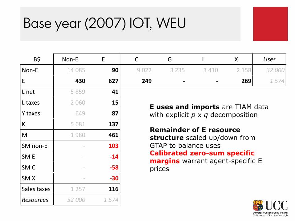
E uses and imports are TIAM data with explicit p x q decomposition

Base year (2007) IOT, WEU
B$ Non-E E C G I X Uses
Non-E 14 085 90 9 022 3 235 3 410 2 158 32 000
E 430 627 249 - - 269 1 574
L net 5 859 41
L taxes 2 060 15
Y taxes 649 87
K 5 681 137
M 1 980 461
SM non-E - 103
SM E - -14
SM C - -58
SM X - -30
Sales taxes 1 257 116
Resources 32 000 1 574
Remainder of E resource structure scaled up/down from GTAP to balance uses
E uses and imports are TIAM data with explicit p x q decomposition
Base year (2007) IOT, WEU
B$ Non-E E C G I X Uses
Non-E 14 085 90 9 022 3 235 3 410 2 158 32 000
E 430 627 249 - - 269 1 574
L net 5 859 41
L taxes 2 060 15
Y taxes 649 87
K 5 681 137
M 1 980 461
SM non-E - 103
SM E - -14
SM C - -58
SM X - -30
Sales taxes 1 257 116
Resources 32 000 1 574
Calibrated zero-sum specific margins warrant agent-specific E prices
E uses and imports are TIAM data with explicit p x q decomposition
Remainder of E resource structure scaled up/down from GTAP to balance uses
Base year (2007) IOT, WEU
B$ Non-E E C G I X Uses
Non-E 14 085 90 9 022 3 235 3 410 2 158 32 000
E 430 627 249 - - 269 1 574
L net 5 859 41
L taxes 2 060 15
Y taxes 649 87
K 5 681 137
M 1 980 461
SM non-E - 103
SM E - -14
SM C - -58
SM X - -30
Sales taxes 1 257 116
Resources 32 000 1 574
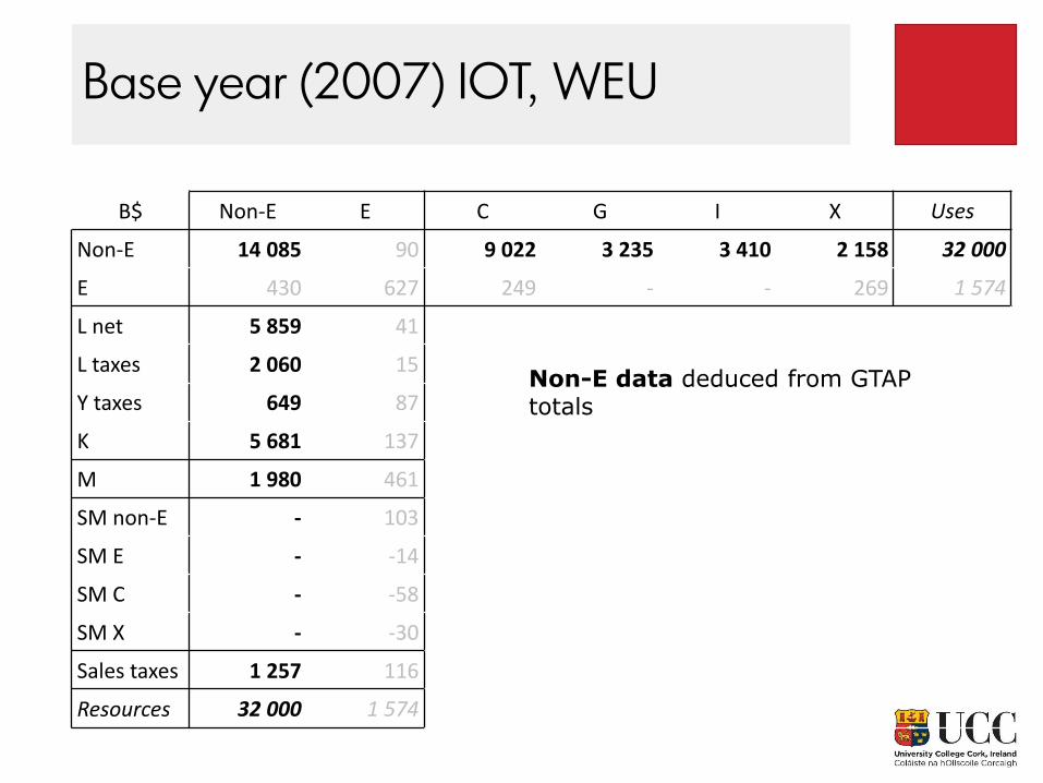
Non-E data deduced from GTAP totals

KLEM behavioural assumptions
• Output sequential trade-off of K vs. L then KL vs. E then KLE vs. ‘M’ (aggregate of non-E goods)• K vs. L, KLE vs. M settled by CES functions
• KL (VA) vs. E from TIAMunder a maintained CES assumption for KLE
• Aggregate savings rate exogenous (recursive dynamics)
• Households’ E consumption from TIAM
• International trade• E trade from TIAM
• Non-E trade: ratio of M to Y isoelastic to terms of trade; X settled by international good CES of exported goods (Armington)
12/16

At each period from 2010 to 2100
B$ Non-E E C G I X Uses
Non-E 14 085 90 9 022 3 235 3 410 2 158 32 000
E ### ### ### - - ### ###
L net 5 859 41
L taxes 2 060 15
Y taxes 649 87
K 5 681 ###
M 1 980 ###
SM non-E - 103
SM E - -14
SM C - -58
SM X - -30
Sales taxes 1 257 116
Resources 32 000 1 574
TIAM trajectory prescribes E uses and imports as well as E investment requirements, which drive KEaccumulation
K rental price adjusts to balance remainder of K supply and K demand by non-E production

At each period from 2010 to 2100
B$ Non-E E C G I X Uses
Non-E 14 085 90 9 022 3 235 3 410 2 158 32 000
E ### ### ### - - ### ###
L net 5 859 ###
L taxes 2 060 ###
Y taxes 649 87
K 5 681 ###
M 1 980 ###
SM non-E - 103
SM E - -14
SM C - -58
SM X - -30
Sales taxes 1 257 116
Resources 32 000 1 574
Labour intensity of E production assumed constant, wage adjusts to balance remainder of L supply and Ldemand by non-E production
Optional imperfect L market magnifies cost of E investment crowding out non-E investment

At each period from 2010 to 2100
B$ Non-E E C G I X Uses
Non-E 14 085 ### 9 022 3 235 3 410 2 158 32 000
E ### ### ### - - ### ###
L net 5 859 ###
L taxes 2 060 ###
Y taxes 649 ###
K 5 681 ###
M 1 980 ###
SM non-E - 103
SM E - -14
SM C - -58
SM X - -30
Sales taxes 1 257 ###
Resources 32 000 1 574
‘M’ (non-E) intensity of E production trades off with KLE aggregate under a constant elasticity of substitution assumption
Output and sales taxes constant ad valorem rates

At each period from 2010 to 2100
B$ Non-E E C G I X Uses
Non-E 14 085 ### 9 022 3 235 3 410 2 158 32 000
E ### ### ### - - ### ###
L net 5 859 ###
L taxes 2 060 ###
Y taxes 649 ###
K 5 681 ###
M 1 980 ###
SM non-E - ###
SM E - ###
SM C - ###
SM X - ###
Sales taxes 1 257 ###
Resources 32 000 ###
Specific margins adjust to have E end-use prices match TIAM agent-specific prices

At each period from 2010 to 2100
B$ Non-E E C G I X Uses
Non-E 14 085 ### 9 022 3 235 3 410 2 158 32 000
E ### ### ### - - ### ###
L net ### ###
L taxes ### ###
Y taxes 649 ###
K ### ###
M 1 980 ###
SM non-E - ###
SM E - ###
SM C - ###
SM X - ###
Sales taxes 1 257 ###
Resources 32 000 ###
In non-E production
K and L trade off with constant elasticity to produce aggregate KL (VA) considering wage and rent adjusted to clear markets
Optional imperfect L market magnifies cost of E investment crowding-out non-E investment
Resulting K, L and E combine into aggregate KLE following CES specification

At each period from 2010 to 2100
B$ Non-E E C G I X Uses
Non-E ### ### 9 022 3 235 3 410 2 158 32 000
E ### ### ### - - ### ###
L net ### ###
L taxes ### ###
Y taxes 649 ###
K ### ###
M 1 980 ###
SM non-E - ###
SM E - ###
SM C - ###
SM X - ###
Sales taxes 1 257 ###
Resources 32 000 ###
In non-E production
Non-E intensity of non-E production and KLE aggregate trade off to produce domestic output Y
The price of the non-E good is the weighted average of domestic and import prices
At each period from 2010 to 2100
B$ Non-E E C G I X Uses
Non-E ### ### 9 022 3 235 3 410 2 158 32 000
E ### ### ### - - ### ###
L net ### ###
L taxes ### ###
Y taxes 649 ###
K ### ###
M ### ###
SM non-E - ###
SM E - ###
SM C - ###
SM X - ###
Sales taxes 1 257 ###
Resources 32 000 ###
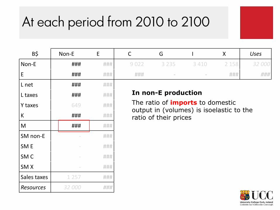
In non-E production
The ratio of imports to domestic output in (volumes) is isoelastic to the ratio of their prices

At each period from 2010 to 2100
B$ Non-E E C G I X Uses
Non-E ### ### 9 022 3 235 3 410 2 158 32 000
E ### ### ### - - ### ###
L net ### ###
L taxes ### ###
Y taxes ### ###
K ### ###
M ### ###
SM non-E - ###
SM E - ###
SM C - ###
SM X - ###
Sales taxes 1 ### ###
Resources 32 000 ###
In non-E production
Exogenous tax rates

At each period from 2010 to 2100
B$ Non-E E C G I X Uses
Non-E ### ### ### ### ### ### ###
E ### ### ### - - ### ###
L net ### ###
L taxes ### ###
Y taxes ### ###
K ### ###
M ### ###
SM non-E - ###
SM E - ###
SM C - ###
SM X - ###
Sales taxes 1 ### ###
Resources ### ###
Final non-E consumptions
G and I are exogenous shares of GDP
X trades off with Xs of other regions at constant elasticity of substitution (Armington) to provide sum of Ms
Closure of accounting balance defines C

Overview of linkage
• TIMES-MACRO (Remme & Blesl, 2006)
• TIAM-KLEM
TIAM
Energy p&qs
KLEM
Labour
ES investment
Households’ consumption
Public consumption
International trade
Investment
Non-E/E Capital
Non-E output
Simultaneously
Iteratively
?Non-E prices?

Harmonising Drivers
• Why? – Initial calibration run not converging with significant differences in BASE calibration
• OECD-SSP2 economic outlook is quite different to existing ETSAP-TIAM macroeconomic drivers.
• SSP2• OECD_SSP2 IIASA-DB
• GDP, POP, Urbanisation
• OECD – ENV-LINKS model Sectoral projections• PAGR, PSERV, PCHEM, PISNF, POEI, POI• OECD in Paris were happy to provide baseline SSP2 consistent Gross
production and value added for results for their GTAP CGE model (25 regions/ 35 sectors)
• World Bank • Historical value added by sector• 2005 – 2010• Full data not available to 2015 yet.

New generation of scenarios
In the lead up to the IPCC’s Sixth Assessment Report new scenarios have been developed to more systematically explore key uncertainties in future socioeconomic developments
Five Shared Socioeconomic Pathways (SSPs) have been developed to explore challenges to adaptation and mitigation. Shared Policy Assumptions (SPAs) are used to achieve target forcing levels (W/m2).
Source: Riahi et al. 2016; IIASA SSP Database; Global Carbon Budget 2016
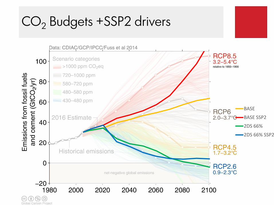
CO2 Budgets +SSP2 drivers
BASE
BASE SSP2
2DS 66%
2DS 66% SSP2

Driver Differences to SSP2
0
10
20
30
40
50
60
70
2000 2025 2050 2075 2100
GDP: AFR
BASE 15R
BASE 15R SSP2
0
5
10
15
20
25
2000 2025 2050 2075 2100
GDP: CHI
0
10
20
30
40
2000 2025 2050 2075 2100
GDP: IND
0
1
2
3
4
2000 2025 2050 2075 2100
GDP: WEU
0
0.5
1
1.5
2
2.5
3
3.5
2000 2025 2050 2075 2100
POP: AFR
BASE 15R
BASE 15R SSP21
1.1
1.2
1.3
1.4
1.5
1.6
2000 2025 2050 2075 2100
POP: IND
0.5
0.7
0.9
1.1
1.3
2000 2025 2050 2075 2100
POP: CHI
0.8
0.9
1
1.1
1.2
2000 2025 2050 2075 2100
POP: WEU

Driver Differences to SSP2
0
20
40
60
80
100
2000 2025 2050 2075 2100
SERV: AFR
BASE 15R
BASE 15R SSP2
0
20
40
60
80
2000 2025 2050 2075 2100
SERV: IND
0
1
2
3
4
5
2000 2025 2050 2075 2100
SERV: WEU
0
50
100
150
200
2000 2025 2050 2075 2100
ISNF: AFR
BASE 15R
BASE 15R SSP2
0
200
400
600
800
2000 2025 2050 2075 2100
ISNF: IND
0
0.5
1
1.5
2
2.5
3
2000 2025 2050 2075 2100
ISNF: WEU
0
10
20
30
40
50
2000 2025 2050 2075 2100
ISNF: CHI
0
5
10
15
20
25
2000 2025 2050 2075 2100
SERV: CHI
??

Primary Energy
0
200
400
600
800
1000
1200
BASE BASE BASESSP2
2DS 66% 2DS 66%SSP2
BASE BASESSP2
2DS 66% 2DS 66%SSP2
2005 2030 2050
ExaJ
ou
les
Coal Oil Gas Nuclear Hydro Biomass Renewable except hydro and biomass
0
500
1000
1500
2000
2500
BASE BASESSP2
2DS66%
2DS66%SSP2
2100
ExaJ
ou
les

Final Energy
-
100
200
300
400
500
600
700
BASE BASE BASESSP2
2DS 66% 2DS 66%SSP2
BASE BASESSP2
2DS 66% 2DS 66%SSP2
2005 2030 2050
ExaJ
ou
les
Coal Oil ProductsGas ElectricityBiomass (excludes liquid biofuels) BiodieselAlcohol Other RenewableHeat Hydrogen
-
200
400
600
800
1,000
1,200
1,400
1,600
BASE BASESSP2
2DS 66% 2DS 66%SSP2
2100Ex
aJo
ule
s

Electricity Capacity
-
2,000
4,000
6,000
8,000
10,000
12,000
14,000
BASE BASESSP2
2DS66%
2DS66%SSP2
BASE BASESSP2
2DS66%
2DS66%SSP2
BASE BASESSP2
2DS66%
2DS66%SSP2
2005 2030 2050
GW
Electricity Generation Installed Capacities (GW)
-
10,000
20,000
30,000
40,000
50,000
60,000
70,000
BASE BASESSP2
2DS66%
2DS66%SSP2
2100
GW
Solar Thermal
Solar PV
Geo, Tidal andWave
Wind
Biomass CCS
Biomass
Hydro
Nuclear
Gas CCS
Gas and Oil
Coal

Electricity Generation
0
20
40
60
80
100
120
140
160
BASE BASE BASESSP2
2DS66%
2DS66%SSP2
BASE BASESSP2
2DS66%
2DS66%SSP2
2005 2030 2050
Exaj
ou
les
Total Electricity Generation
0
100
200
300
400
500
600
BASE BASESSP2
2DS66%
2DS66%SSP2
2100
Exaj
ou
les
SolarThermalSolar PV
Geo, Tidaland WaveWind
BiomassCCSBiomass
Hydro
Nuclear
CH4OptionsGas CCS
Gas andOil
KLEM eventual Outputs
• GDP change
• Consumption change across sectors
• Employment change
• Re-estimated output/drivers • Residential,
• Energy firms
• Non-Energy – Commercial/Services

Conclusions
• This hybrid type of approach steps towards sectoral specific dynamics of decarbonising from a bottom up technology explicit perspective• Unemployment, structural changes, sectoral outputs, drivers
• A broader approach to assess demand uncertainty using the SSP narratives could be integrated into TIAM/regional/or National Models• A CGE such as KLEM or GTAP is required to generate sectoral SSP drivers.
(disaggregate GDP)• Is it appropriate that we generally don’t have multiple drivers scenarios?• Long term OECD-SSP2 drivers cause extreme growth indices post 2060 in
emerging economies. – review elasticities…
• A Hybrid (GE) TIAM is ideal for NDC analysis given TIAM’s bottom up nature and a hybrid general equilibrium with the economy.• Technology specific NDCs - USA• Economic Intensity NDCs - INDIA/CHINA• Carbon limits - Europe

Environmental Research InstituteInstiúd Taighde Comshaoil
Energy Policy and Modelling Groupwww.ucc.ie/energypolicy
@james_glynn

Lahinch Beach, Co Clare, IRELAND– Monday, January 6th
Thanks youQUESTIONS?

@james_glynn is a Postdoctoral researcher in @MaREIcentre @ERIUCC @UCC
working on global integrated assessment models linking detailed energy-economy-climate
models, to assess equitable, ambitious and secure decarbonisation of the energy system
eMail: [email protected]
Twitter: @james_glynn
Web: www.ucc.ie/energypolicy
Profile: http://www.ucc.ie/en/energypolicy/people/jamesglynn/

Energy Policy & Modelling Collaborators and Funders

GLOBAL ETSAP-TIAM model
• Linear programming bottom-up energy system model of IEA-ETSAP
• Integrated model of the entire energy system
• Prospective analysis on medium to long term horizon (2100)• Demand driven by exogenous energy service demands
• Partial and dynamic equilibrium (perfect market)
• Optimal technology selection
• Minimizes the total system cost
• Environmental constraints• Integrated Climate Model
• 15 Region Global Model
• Price-elastic demands
• Macro Stand Alone• Single consumer-producer, multi-regional, inter-temporal general equilibrium model which
maximises regional utility.• The utility is a logarithmic function of the consumption of a single generic consumer.• Production inputs are labour, capital and energy.• Energy demand and energy costs from ETSAP-TIAM model.• MSA Re-estimates Energy Service Demands based on energy cost

IPCC INDC Synthesis Report

ETSAP-TIAMReference Energy System
Source: Loulou, R., Labriet, M., 2008. ETSAP-TIAM: the TIMES integrated assessment model Part I: Model structure. Comput. Manag. Sci. 5, 7–40. doi:10.1007/s10287-007-0046-z

ETSAP-TIAM 15 Regions
AFR
CAN
USA
MEX
CSA
WEU
EEU
MEA
IND
CHISKO
JPN
AUS
ODA

GDP losses & Costs of Delayed Action
0 2 4 6 8 10 12 14 16 18 20
2DS 50%
2DS 50% DA20
2DS 50%
2DS 50% DA20
2DS 50%
2DS 50% DA20
2DS 50%
2DS 50% DA20
20
30
.2
05
0.
20
70
.2
10
0
GDP Loss %
Former Soviet Union
Australia & NZ
South Korea
Other Developing Asia
Canada
Middle East
China
East Europe
Africa
India
West Europe
Japan
USA
Central South America
Mexico

ETSAP-TIAM MSA (TMSA)Macro Stand Alone
𝑀𝑎𝑥 𝑈 =
𝑡=1
𝑇
𝑟
𝑛𝑤𝑡𝑟 . 𝑝𝑤𝑡𝑡. 𝑑𝑓𝑎𝑐𝑡𝑟,𝑡. 𝑙𝑛 𝐶𝑟,𝑡 (1) (MSA OBJz)
𝑌𝑟,𝑡 = 𝐶𝑟,𝑡 + 𝐼𝑁𝑉𝑟,𝑡 + 𝐸𝐶𝑟,𝑡 + 𝑁𝑇𝑋(𝑛𝑚𝑟)𝑟,𝑡 (2)
𝑌𝑟,𝑡 = 𝑎𝑘𝑙𝑟 ∙ 𝐾𝑟,𝑡𝑘𝑝𝑣𝑠𝑟∙𝜌𝑟 ∙ 𝑙𝑟,𝑡
(1−𝑘𝑝𝑣𝑠𝑟)𝜌𝑟 +
𝑘
𝑏𝑟,𝑘 ∙ 𝐷𝐸𝑀𝑟,𝑡,𝑘𝜌𝑟
1𝜌𝑟
(3)
• nwt – Negishi Weights
• pwt – weight Multiplier
• dfact – utility discount factor
• C - Consumption
• Y – Production
• INV – Investment
• EC – Energy Cost
• NTX – Net exports
• akl – production fn constant
• K – Capital
• kpvs – capital value share
• l - Labour annual growth
• b – Demand coefficient
• p – elasticity of substitution
• DEM - Energy Demands
R
r YEARSy
yREFYR
yr yrANNCOSTdNPVMin1
, ),()1( (TIAM OBJz)

TIMES Energy System Model
Cost and emissions balance
GDP
Process
Heating area
Population
Light
Comms
Power
Person kilometers
Freight kilometers
Service Demands
Coal processing
Refineries
Power plantsand
Transportation
CHP plantsand district
heat networks
Gas network
Industry
Commercial and
Tertiary
Households
Transport
Final energyPrimary energy
Domesticsources
Imports
De
ma
nd
sE
ne
rgy p
rice
s, R
eso
urc
e a
vaila
bili
ty