linking surface- and ground-water levels to … · clements’ community-unit theory (clements...

665

WETLANDS, Vol. 24, No. 3, September 2004, pp. 665–687q 2004, The Society of Wetland Scientists

LINKING SURFACE- AND GROUND-WATER LEVELS TO RIPARIANGRASSLAND SPECIES ALONG THE PLATTE RIVER IN

CENTRAL NEBRASKA, USA

Robert J. Henszey1,3, Kent Pfeiffer1, and Janet R. Keough2,4

1 Platte River Whooping Crane Maintenance Trust6611 W. Whooping Crane Dr.

Wood River, Nebraska, USA 68883

2 United States Geological SurveyNorthern Prairie Wildlife Research Center

8711 37th St. SoutheastJamestown, North Dakota, USA 58401

3 Present address:U.S. Fish and Wildlife Service

Fairbanks Fish and Wildlife Field Office101 12th Ave., Box 19, Room 110

Fairbanks, Alaska, USA 99701E-mail: [email protected]

4 Present address:U.S. Environmental Protection Agency

National Health and Environmental Effects Research Laboratory Mid-Continent Ecology Division6201 Congdon Blvd.

Duluth, Minnesota, USA 55804

Abstract: Nearly all the techniques used to quantify how plants are linked to environmental gradientsproduce results in general terms, such as low to high elevation, xeric to mesic, and low to high concentration.While ecologists comprehend these imprecise scales, managers responsible for making decisions affectingthese gradients need more precise information. For our study, we preserved the measurement scale and unitsof a dominant environmental gradient by using non-linear models to fit plant frequency to a water-levelgradient ranging from shallow ground water to standing water along the Platte River in central Nebraska,USA. Non-linear models, unlike polynomials, have coefficients that can be interpreted with a biologicalmeaning such as population peak, optimum gradient position, and ecological amplitude. Sixty-three ripariangrassland species had sufficient information to link their plant frequency to the water-level gradient. Fromamong 10 water-level summary statistics evaluated for a subset of 22 species, the best plant-frequencyresponse curves were obtained by using the growing season 10% cumulative frequency water level, followedclosely by the growing season 7-day moving average high water level and two other high water-levelstatistics. This suggests that for Platte River riparian grasslands, high water levels are more influential thanmean, median, or low water levels. Land-management practices (i.e., grazing, haying, and extended rest)affected six species by a change in frequency or a shift in position along the water-level gradient. Fourgeneral plant communities composed of species responding individually to the water-level gradient and otherfactors were identified for Platte River riparian grasslands: emergent, sedge meadow, mesic prairie, and dryridge. Plant response curves are the first step toward predicting how plants responding to riparian-grasslandwater levels might also respond to river management.

Key Words: riparian vegetation, wet meadow, direct gradient analysis, species response curve, non-linearmodels, surface- and ground-water level, water table, plant frequency, coenocline

INTRODUCTION

Ecologists began quantifying ecological gradients inthe first half of the 20th century by first describing spe-cies relationships to environmental gradients (e.g.,Shreve 1922, Wells 1928) and later by fitting mathe-

matical expressions (e.g., Gause 1930, 1931, 1932).By the mid-20th century, gradients were used by Whit-taker (1951, 1956) in support of Gleason’s individu-alistic hypothesis (Gleason 1926, 1939) to challengeClements’ community-unit theory (Clements 1916,

666 WETLANDS, Volume 24, No. 3, 2004

Figure 1. An example of a biplot from a canonical corre-spondence analysis of the data for our study. Note how thespecies can be ranked along an environmental gradient byextending a perpendicular line to the gradient axis (vectorradiating from the origin with only the positive side shown),but there is no information on how each species is distrib-uted along the gradient. The length and angle of the envi-ronmental vectors shows their importance and their relation-ship with other gradients. The eigenvalues representing thevariance attributed to Axes 1 and 2 are 0.605 and 0.221.Parts per million phosphorus (P), percent clay content(%Clay), salinity, organic matter (OM), and pH are from acompanion study by Simpson (2001), while the surface wa-ter content (SurMoist) and the growing season 7-day movingaverage high water level (7-DayHI) are from our study. Axis1 is correlated with water availability (7-DayHI, SurMoist)and water-mediating gradients (Salinity, OM, %Clay) andcan be considered a gradient from nearly hydric to almostxeric, while Axis 2 with less than half the explained variancecan be considered a pH gradient. The ellipses represent ap-proximate plant community boundaries.

1936). At about this same time, Whittaker was alsorefining direct gradient analysis techniques to describeplant species responses along predetermined environ-mental gradients such as pH, while Curtis and his as-sociates were developing indirect gradient analysistechniques to arrange species along axes of variationbased on the degrees of difference in plant speciescomposition (Whittaker 1967). Both techniques can in-corporate multiple gradients or axes, although higherdimensional analyses can be difficult to visualize with-out a graphical technique similar to biplots (e.g., Fig-ure 1), which use vector lengths and angles radiating

from a centroid to represent gradients (ter Braak 1986).Toward the latter part of the 20th century, plant re-sponse curves from actual and simulated gradientswere used in simulation modeling to gain valuable in-sights into plant community ecology (e.g., Gauch andWhittaker 1972, Palmer 1992, Seabloom et al. 2001).

Nearly all these techniques and analyses produce re-sults that represent environmental gradients (whichmay be measured quantitatively) in general terms, suchas low to high elevation, xeric to mesic, and low tohigh concentration (e.g., Figure 1). While ecologistsunderstand the implications of these imprecise scales,managers responsible for making decisions affectingone or more of these gradients need information thatis more precise. For example, specifying that mesicconditions are necessary to maintain a particular plantcommunity is much less informative than specifyingthat the community requires a water table within 10cm of the surface for seven consecutive days eachyear.

In this paper, we preserve the measurement scaleand units of a dominant environmental gradient by us-ing non-linear models to fit plant-species responsecurves to a water-level gradient ranging from shallowground water to standing water. Non-linear models aremore useful than linear models, like polynomials, be-cause their coefficients can be interpreted with a bio-logical meaning such as population peak, optimumgradient position, and ecological amplitude. Note thatthe term ‘‘linear’’ refers to the linear arrangement ofthe parameter coefficients in the model, not the shapeof the curve (AISN Software Inc. 2000). A linear mod-el can describe very complex curves, possibly fittingthe data better than a non-linear model, but the linearcoefficients have little biological meaning. One of theearliest and by far the most frequently used models tofit plant response to gradients is the Gaussian model(Gause 1931, 1932, Austin 1976). This non-linearmodel produces the familiar symmetrical bell-shapedcurve and has been used by many investigators (e.g.,Gause 1932, Whittaker 1956). Several investigators(e.g., Austin and Austin 1980, Werger et al. 1983,Austin 1987, Minchin 1987), however, have criticizedthe Gaussian model because there appears to be nobiological basis for a symmetric response. Indeed,many species appear to show an asymmetric (skewed)or possibly platykurtic (plateau shaped) or even bi-modal (more than one peak) response. One solution tothis debate is to use a versatile non-linear model likethe beta model, which can produce symmetric, asym-metric, and platykurtic curves (Austin 1976, Minchin1987). Since there is still some debate over the ‘‘best’’model(s) to fit plant responses to an environmentalgradient, we tested the Gaussian and beta models along

Henszey et al., LINKING WATER LEVELS TO RIPARIAN GRASSLAND SPECIES 667

Figure 2. Map of the study areas and sampling sites alongthe Platte River in south central Nebraska, USA.

with 52 other non-linear models to obtain a best-fitplant response curve.

Our study was conducted in the riparian grasslandsalong the Platte River in central Nebraska, USA (Fig-ure 2). These grasslands support a multitude of migra-tory birds and are being considered as part of a three-state, basin-wide, riverflow re-regulation plan to en-hance migratory habitat for the endangered whoopingcrane (Cooperative Agreement 1997). This area offerslow undulating topography with approximately 2 m ofrelief, which provides repeating water-level gradientsranging from standing water to approximately 3 m be-low the surface as the topography varies from sloughsto ridge tops. A study by Simpson (2001) used canon-ical correspondence to identify surface- and ground-water levels as the primary gradient in these grass-lands, followed by salinity and phosphorus fromamong 12 parameters for hydrology, nutrients, organicmatter, and soil texture. Our goal was to refine theplant response to surface- and ground-water levels fur-ther as a first step toward determining what influenceriver stage might have on these water levels and, inturn, on the plant species and communities.

METHODS

Study Area

The Platte River in central Nebraska, USA(408499N, 988239W) lies within the Central GreatPlains ecoregion at 575–635 m elevation and is a wide,braided, shallow, low-gradient sand-bed river thatdrains approximately 137,000 km2 from the states ofColorado, Wyoming, and Nebraska (Omernik 1987,Hitch et al. 2002). Mean annual precipitation withinthe study area is about 630 mm (National ClimaticData Center 2000). Mean monthly riverflows rangefrom nearly bank full in June (72 m3s21) to substantialareas of exposed riverbed in August (18 m3s21, Hitch

et al. 2002). Much of the area formerly occupied byriparian grasslands within the Platte River valley, re-ferred locally as wet meadows, has been converted tocropland (Sidle et al. 1989). The majority of remainingriparian grasslands now exist primarily as remnantswithin a matrix of agricultural land located within 3km of the channel. These riparian grasslands are char-acterized by high water tables, slow runoff, nutrient-rich soils, and an undulating topography reminiscentof the braided channels from which they were formed.The principal aquifer within the Platte River valley iscomposed of unconfined Pleistocene sands and gravels(Schreurs and Rainwater 1956) and is recharged by theriver and by precipitation (Hurr 1983, Wesche et al.1994). Moderate to highly permeable soils (K 5 5 to.50 cm·hr21), from 13–43 cm deep, formed in theloamy or sandy alluvium deposited over this highlypermeable aquifer (Advanced copy, Hall County soilsurvey update, USDA Natural Resources ConservationService, Grand Island, NE). Above the water table,saturated conditions are probably insignificant, sincethe coarse sands and gravels minimize the capillaryfringe, and the highly permeable soil allows infiltratedprecipitation to quickly pass through to the water table(USDA, NRCS, Soil Survey Division 2003).

Sample sites were located along a 50-km reach ofthe Platte River between Kearney and Grand Island,Nebraska (Figure 2). All sites were managed by thePlatte River Whooping Crane Maintenance Trust, ex-cept that the Rowe Sanctuary sites were managed bythe National Audubon Society and the Binfield sitewas managed by a private landowner. Land-manage-ment practices included livestock grazing rotations,hay rotations, and extended rest (4 to 8 years). Stock-ing rate varied by management unit but was typicallyabout 0.3 animal unit months per hectare. All threepractices also included periodic prescribed burns aspart of their management. Since it was impractical tosample all combinations of these management practic-es (e.g., early or late grazing, and burned or unburned),we chose to limit our analysis to three broad-basedmanagement practices: grazed, hayed, or extendedrested.

Study Design and Analyses

A three-step process was used to link surface- andground-water levels to plant response: describe theseasonal water-level pattern, describe the plant speciesfrequency, and finally fit a curve through the data toquantify the linkage between water levels and plantfrequency. The general procedure included samplingplant species frequency along a water-level gradientfrom the bottom of a swale to the top of an adjacentridge (;200 cm change in relative elevation, Figure


Figure 3. Cross-section profiles for one of the multiple-swale sites showing how an additional swale-ridge profile(Gradient 1B) was used to extend the surface- and ground-water-level gradient up slope. Four of the 12 replicates (threehayed and one rested) required an additional swale-ridgeprofile located from 0.2 to 18 km away to complete theirwater-level gradient. The two wells for each profile wereused to determine the water-level slope between wells. Veg-etation sampling transects were located at 15-cm intervals inrelative elevation starting from near the bottom of eachswale.

3). Several distinct plant communities occur along thisgradient as individual species express their response tooptimum water levels. Sample sites (individual swale-ridge profiles) were selected during the summer of1998 to represent four replicates of the three broad-based land-management practices (grazed, hayed, orrested) and to represent the full water-level gradienttypical for native Platte River riparian grasslands(about 150 to 2200 cm relative to the land surface,where positive values are surface water and negativevalues are ground water). Ideally, each replicate shouldonly need one swale-ridge profile to cover the full wa-ter-level gradient, but in practice, four replicates (threehayed and one rested) required an additional ‘‘higher’’swale located from 0.2 to 18 km away to extend thewater-level gradient up slope (e.g., Figure 3). Thecompleted study design, therefore, consisted of 16sample sites: four grazed, seven hayed, and five rested.

Water-Level Pattern. Each study site had a pair ofshallow observation wells, one located near the bottomof the swale and one located near the top of an adja-cent ridge (Figure 3). These wells were used to deter-mine the water-level slope between the wells and toestimate the water-level gradient (i.e., surface orground-water depth) from the bottom of the swale tothe top of an adjacent ridge. Most wells were installedto Nebraska state standards (Nebraska Health and Hu-man Services 1999) using 5.1-cm-diameter schedule40 polyvinyl chloride casings with the lower 150 cmscreened and open to the aquifer, and a 60-cm-thick

bentonite seal placed above the water table. The re-maining wells were previously installed by Wesche etal. (1994) with less stringent standards (e.g., no ben-tonite seal, hand-made screens) but were consideredsuitable for monitoring the shallow water table. Allwater levels were measured biweekly to the nearest 0.3cm (0.01 ft) using a fiberglass tape equipped with anelectronic sensor (Henszey 1991), except during thewinter when they were measured monthly. At least onewell at each site was also equipped with a continuouswater-level recorder. Continuous water levels for thenon-recording wells were estimated by regression withthese adjacent recording wells. Linear interpolation be-tween each pair of wells was then used to estimatecontinuous water levels for the vegetation transects lo-cated between the bottom of the swale and the top ofan adjacent ridge. If the interpolation predicted surfacewater in the swale, then the surface-water level wasfurther adjusted to account for excess runoff or run-onby regression with the surface-water levels observedfor that swale during the periodic biweekly and month-ly measurements. Precipitation and evapotranspirationwere continuously monitored onsite by four weatherstations and five recording rain gages. These gageswere located so that all sample sites were within 4.4km of a weather station and 0.8 km of a rain gage.

Since no single water-level summary statistic canadequately describe the complex pattern of seasonalwater levels, we chose to evaluate three types of sum-mary statistics (cumulative frequencies, moving aver-ages, and arithmetic mean) as appropriate statistics forlinking surface- and ground-water levels to plant fre-quency. Before calculating these summary statistics,the continuous water levels were first summarized asmean daily water levels for each 24-hour period. Thisminimized transient diurnal fluctuations caused by dai-ly cycles of evapotranspiration and other factors,which are probably much less important to plants thanthe mean daily water level. Mean daily water levelswere then summarized for each vegetation transect us-ing the summary statistics for the 1999 and 2000growing seasons (15 March to 15 October; e.g., Figure4).

Cumulative frequency distributions (e.g., Zarr 1974)show the number of days (i.e., the percent of time)during the growing season that the water was at orabove a particular level, similar to the streamflow-du-ration curves (Searcy 1959) used by hydrologists. Wa-ter levels at the 10%, 50% (median), and 90% cumu-lative frequency for mean daily water level were cho-sen to test for plant-response linkages (L10%, L50%, L90%),since these levels represent what might be called thetypical high, median, and low water levels for thegrowing season. The actual highest and lowest mean-daily water levels for the growing season would be the


Figure 4. Water-level pattern and summary statistics forone well during the 2000 growing season (15 March to 15October). The mean daily water level is the average waterlevel for each 24-hour period and is already a summary ofthe instantaneous water level, which is too transitory forsummarizing seasonal water levels. The 7-day moving av-erage removes some of this variability and takes into accountpreceding water levels by averaging the mean daily waterlevel for the current and previous six days. The cumulativefrequency of mean daily water levels eliminates the timesequence altogether by showing the percent of days duringthe growing season that the water was at or above a partic-ular level.

0% and 100% cumulative frequency values respec-tively. For example, in Figure 4, the 10% cumulativefrequency for mean daily water levels was 8 cm, show-ing that for 10% of the growing season (22 of 215days), the water was at or above 8 cm above the sur-face. Likewise, the 90% cumulative frequency formean daily water levels was 270 cm, showing that thewater was at or above 70 cm below the surface for90% of the growing season (194 of 215 days). Al-though this 90% value might not seem to be too usefulsince it covers a considerable portion of the growingseason, the cumulative frequency scale can be easilyreversed so that the 90% value also represents the val-ue for 10% of the growing season when the mean dailywater level was below a particular level (e.g., 270cm). Cumulative frequencies are useful for describinghow often the water was at or above a specific level,but they do not represent the actual sequence of ob-served events. For example, in Figure 4, the mean dai-ly water level was at or above the land surface for17% of the growing season (37 of 215 days), but thatpercentage was distributed across three periods ofwidely different duration and for at least some portionof March, April, and May.

Moving-average water levels for 7, 10, and 14 days(L7, L10, L14) were also tested to determine if an averageof the immediately preceding mean daily water levelsmight be more important to plants than simply how

often the water was at or above a particular level dur-ing the growing season. Moving averages can be cal-culated in a variety of ways (e.g., Shumway and Stof-fer 2000), but we chose to calculate a simple movingaverage (Ln) by averaging the mean daily water levelfor the current (Lt) and previous number (n 2 1) ofdays:

1L 5 [L 1 L 1 · · · 1 L ],n t t21 t2(n21)n

where Ln is the current moving-average water level attime t and n is the number of days used to calculatethe moving average. For testing plant response link-ages, the n-day high and low moving-average waterlevels for the growing season (LnH and LnL) were cho-sen, like the 10% and 90% cumulative frequencies,because they may represent periods of high or lowwater-level stress for plants. Unlike the cumulative fre-quencies, however, the n-day moving averages can beassociated with a date (or dates). For example, in Fig-ure 4, the growing season 7-day moving average highwater level (L7H) was 12 cm above the surface for 25March, while the growing season 7-day moving av-erage low water level (L7L) was 76 cm below the sur-face on 19 September. While not specifically intendedto meet any particular standard for wetland hydrology(National Research Council 1995), the L10H closely ap-proximates the 5% criterion of the 1987 Corps manual(Environmental Laboratory 1987), the L7H meets the1989 interagency manual criterion (Federal Interagen-cy Committee for Wetland Delineation 1989), and theL14H approximates the 15-day criterion for the 1991proposed revisions (U.S. Environmental ProtectionAgency et al. 1991).

The arithmetic mean is simply the mean water levelfor the growing season (LS) and, together with the L50%,is a measure of the central tendency or ‘‘average’’growing season water level. Growing season high wa-ter levels are represented by L10%, L7H, L10H, L14H, whilethe growing season low water levels are representedby L90%, L7L, L10L, L14L None of these statistics, however,consider the root zone. The standard normal deviate(Hunt et al. 1999) is one high water-level statistic thatconsiders the root zone but was not tested here becauseour water levels never entered the root zone on theupslope end of the water-level gradient. The standardnormal deviate measures the root zone residence timeby using a cumulative frequency to summarize thenumber and duration of contiguous periods when thewater level was at or above the root zone (typicallywithin 30 cm below the land surface). This statisticcombines aspects of the cumulative frequency and themoving average, and it should be considered for stud-ies where the water level consistently enters the root


Figure 5. An example of a non-linear model used to fit atheoretical plant response to an environmental gradient witharbitrary units. Note how the coefficients can be interpretedwith a biological meaning (e.g., a 5 amplitude of the peakplant response, b 5 water level at the peak, and FWHM 5an indication of the range of favorable water levels at halfthe peak response). The full width at half-maximum(FWHM) is a function of c.

zone (i.e., wetlands and possibly shallow subirrigatedplant communities).

Plant Response. Vegetation transects aligned alongtopographic contours were established at 15-cm incre-ments in relative elevation from the bottom of eachswale to the top of an adjacent ridge (Figure 3) usinga rotating laser level. Transects were marked with athin polypropylene line interwoven with stainless steelthreads so the transects could be relocated in subse-quent years, even after a prescribed burn. Two hundredpoints per transect, spaced 10 cm apart, were used tocalculate plant frequency by species based on the near-est plant to each point. This technique for botanicalcomposition is similar to Evans and Love (1957) andOwensby (1973), except that a 10-pin point frame wasplaced sequentially along a relatively short transect(i.e., 20 m) to stay within a reasonable distance (610m) of the water-level gradient between the wells, rath-er than single points along a longer transect (e.g., 100m). Starting points were randomly selected from with-in the first meter of the transect’s downstream end.Although frequency has some limitations (Mueller-Dombois and Ellenberg 1974), we chose this metricinstead of canopy cover or biomass because frequencyis less affected by plant phenology or by herbage re-moval from grazing or haying. To minimize pheno-logical effects on plant frequency, sampling was con-ducted in the early summer of 1999 and 2000 whilethe early-flowering sedges (Carex spp.) were still iden-tifiable to species and the warm season species hademerged sufficiently to be identified. Frequency for pe-rennials, like the vast majority of Platte River speciesevaluated, is slower to respond to environmental fluc-tuations about a seasonal norm than canopy cover orbiomass, so the two years cannot be considered inde-pendent samples. Thus, the mean frequency for 1999and 2000 by transect, and the associated mean water-level statistic, was considered the experimental unit.Nomenclature follows the PLANTS database (USDA,NRCS 2001), based on the taxonomy by Great PlainsFlora Association (1986), Rolfsmeier (1995), andRolfsmeier and Wilson (1997).

Linking Water Levels to Plant Response. Direct gra-dient analysis (e.g., Whittaker 1967) by fitting a non-linear curve through the data was used to evaluate po-tential links between water levels and plant speciesfrequency. Non-linear models were used because theircoefficients can be interpreted with a biological mean-ing (e.g., amplitude of the peak plant response, waterlevel at the peak, and an indication of the range offavorable water levels; Figure 5). Complex polyno-mials (e.g., y 5 a 1 b1x 1 b2x2 1 b3x3 1 . . . 1 bnxn),on the other hand, may provide a better fit to the data,but their coefficients typically have little or no biolog-

ical meaning. Models were fit to the data with an au-tomated curve fitting software program (AISN Soft-ware Inc. 2000), which can simultaneously fit 12 sym-metrical and 25 asymmetrical non-linear peak models,as well as four symmetrical and 11 asymmetrical non-linear transition (sigmoid shape) models. The rankingof these models, however, does not include a com-bined test for model fit and a penalty for over-speci-fying the model by using more parameters than nec-essary, so we used the corrected Akaike informationcriterion (AICc, Burnham and Anderson 1998) to rankthe models. AICc incorporates the residual sum ofsquares, the number of parameters, and the samplesize, so that the model with the lowest AICc indicatesthe best fit from within the set of models evaluated.Since AICc values occur on a relative scale specific tothe data, we computed corrected Akaike informationcriterion differences (Di 5 AICci 2 minimum AICc) tofacilitate interpretation and to allow quick comparisonand ranking of the candidate models by rescaling theAICc values (Burnham and Anderson 1998). Burnhamand Anderson (1998) suggest that as a rough rule ofthumb models are essentially the same with a Di # 2,models have considerably less support for Di valuesbetween about 4 to 7, and models have essentially nosupport for Di values greater than 10. The responsibil-ity for selecting appropriate models to evaluate, how-ever, is up to the investigator. Since we did not havean a priori knowledge of which non-linear modelsmight be appropriate, we tested all 52 non-linear mod-els, including the Gaussian and beta models used byprevious investigators (e.g., Gause 1931, 1932, Austin1976, Minchin 1987). This occasionally produced a


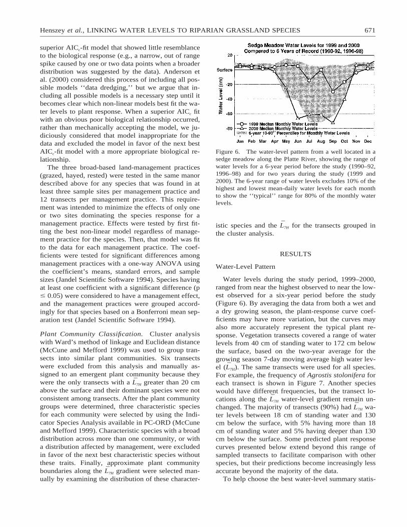
Figure 6. The water-level pattern from a well located in asedge meadow along the Platte River, showing the range ofwater levels for a 6-year period before the study (1990–92,1996–98) and for two years during the study (1999 and2000). The 6-year range of water levels excludes 10% of thehighest and lowest mean-daily water levels for each monthto show the ‘‘typical’’ range for 80% of the monthly waterlevels.

superior AICc-fit model that showed little resemblanceto the biological response (e.g., a narrow, out of rangespike caused by one or two data points when a broaderdistribution was suggested by the data). Anderson etal. (2000) considered this process of including all pos-sible models ‘‘data dredging,’’ but we argue that in-cluding all possible models is a necessary step until itbecomes clear which non-linear models best fit the wa-ter levels to plant response. When a superior AICc fitwith an obvious poor biological relationship occurred,rather than mechanically accepting the model, we ju-diciously considered that model inappropriate for thedata and excluded the model in favor of the next bestAICc-fit model with a more appropriate biological re-lationship.

The three broad-based land-management practices(grazed, hayed, rested) were tested in the same manordescribed above for any species that was found in atleast three sample sites per management practice and12 transects per management practice. This require-ment was intended to minimize the effects of only oneor two sites dominating the species response for amanagement practice. Effects were tested by first fit-ting the best non-linear model regardless of manage-ment practice for the species. Then, that model was fitto the data for each management practice. The coef-ficients were tested for significant differences amongmanagement practices with a one-way ANOVA usingthe coefficient’s means, standard errors, and samplesizes (Jandel Scientific Software 1994). Species havingat least one coefficient with a significant difference (p# 0.05) were considered to have a management effect,and the management practices were grouped accord-ingly for that species based on a Bonferroni mean sep-aration test (Jandel Scientific Software 1994).

Plant Community Classification. Cluster analysiswith Ward’s method of linkage and Euclidean distance(McCune and Mefford 1999) was used to group tran-sects into similar plant communities. Six transectswere excluded from this analysis and manually as-signed to an emergent plant community because theywere the only transects with a L7H greater than 20 cmabove the surface and their dominant species were notconsistent among transects. After the plant communitygroups were determined, three characteristic speciesfor each community were selected by using the Indi-cator Species Analysis available in PC-ORD (McCuneand Mefford 1999). Characteristic species with a broaddistribution across more than one community, or witha distribution affected by management, were excludedin favor of the next best characteristic species withoutthese traits. Finally, approximate plant communityboundaries along the L7H gradient were selected man-ually by examining the distribution of these character-

istic species and the L7H for the transects grouped inthe cluster analysis.

RESULTS

Water-Level Pattern

Water levels during the study period, 1999–2000,ranged from near the highest observed to near the low-est observed for a six-year period before the study(Figure 6). By averaging the data from both a wet anda dry growing season, the plant-response curve coef-ficients may have more variation, but the curves mayalso more accurately represent the typical plant re-sponse. Vegetation transects covered a range of waterlevels from 40 cm of standing water to 172 cm belowthe surface, based on the two-year average for thegrowing season 7-day moving average high water lev-el (L7H). The same transects were used for all species.For example, the frequency of Agrostis stolonifera foreach transect is shown in Figure 7. Another specieswould have different frequencies, but the transect lo-cations along the L7H water-level gradient remain un-changed. The majority of transects (90%) had L7H wa-ter levels between 18 cm of standing water and 130cm below the surface, with 5% having more than 18cm of standing water and 5% having deeper than 130cm below the surface. Some predicted plant responsecurves presented below extend beyond this range ofsampled transects to facilitate comparison with otherspecies, but their predictions become increasingly lessaccurate beyond the majority of the data.

To help choose the best water-level summary statis-


Figure 7. Fitting the frequency of Agrostis stolonifera tothe growing season 7-day moving average high water level(L7H) with a Complementary Error Function Peak equationby using the mean of two years of data from 131 vegetationtransects. Note how the coefficients can be interpreted witha biological meaning: a 5 peak frequency, b 5 location ofpeak along the water-level gradient L7H, and 1.38c 5 fullwidth at half-maximum (FWHM—a measure of ecologicalamplitude at half the peak frequency). CI is the 95% confi-dence interval for b.

Table 1. Ranking water-level summary statistics, using the average corrected Akaike information criterion differences (Di) for a subsetof 22 species.* The growing season 10% cumulative frequency water level (L10%) produced the best summary statistic for these 22 species,but any water-level statistic with a Di # 2 (Burnham and Anderson 1998) could be considered equally suitable for linking water levelsto plant frequency.

Water-Level StatisticAverage AICc

Di Rank

Growing Season High Water-Level Statistics

10% Cumulative Frequency (L10%)7-day Moving Average High (L7H)10-day Moving Average High (L10H)14-day Moving Average High (L14H)

00.10.91.0

1234

Growing Season Central Tendency Water-Level Statistics

50% Cumulative Frequency (L50%)Arithmetic Mean (LS)

3.96.5

56

Growing Season Low Water-Level Statistics

90% Cumulative Frequency (L90%)7-day Moving Average Low (L7L)10-day Moving Average Low (L10L)14-day Moving Average Low (L14L)

13.215.214.213.5

71098

* Subset of species tested: Agrostis stolonifera, Andropogon gerardii, Apocynum cannabinum, Calamagrostis stricta, Calamovilfa longifolia, C. crawei,C. duriuscula, C. emoryi, C. pellita, C. praegracilis, C. tetanica, Eleocharis palustris, Leersia oryzoides, Lycopus asper, Panicum virgatum, Phylalanceolata, Polygonum amphibium, Sorghastrum nutans, Spartina pectinata, Symphyotrichum lanceolatum, Verbena stricta, Viola nephrophylla.

tic for linking water levels to plant frequency, all 10water-level summary statistics were used to fit re-sponse curves to a subset of 22 species. Table 1 sum-marizes these results by averaging corrected Akaikeinformation criterion differences (Di) for each water-level summary statistic. Based on Burnham and An-derson’s (1998) rough rule of thumb that models are

essentially the same with a Di # 2, the four growingseason high water-level statistics (L10%, L7H, L10H, L14H)provide much better links to plant frequency than theother water-level statistics. The two growing seasoncentral tendency water-level statistics (L50%, LS), whichare commonly used to summarize water levels, haveconsiderably less support for linking plant frequency,since their Di values are between about 4 to 7. Thefour growing season low water-level statistics (L90%,L7L, L10L, L14L) have essentially no support for linkingplant frequency, since their Di values are greater than10. Although any of the four growing season high wa-ter-level statistics could be used to link water levels toplant frequency without much information loss, wechose to use the best statistic that has an equivalent inany current or proposed standard, the L7H, which meetsthe 1989 interagency manual criterion for wetland hy-drology.

It might be helpful to put the 7-day moving averagehigh water level (L7H) into terms of the currently used1987 Corps manual for delineating jurisdictional wet-lands. Based upon the L10H, which approximates the1987 Corps criteria, the 1987 Corps 5% soil saturationcriteria for the growing season (10.75 of 215 days forour sites) would be three days longer (10 instead of 7consecutive days) and about 2.5 cm lower than the L7H

water levels presented below. Although the L7H is notrestricted to the 30-cm regulatory root zone depth, the2.5 cm difference in water levels suggests that the reg-ulatory depth for the L7H would be about 27.5 cm.Thus, the L7H used in this paper is a little less stringent


than the 1987 Manual for the number of consecutivedays, and the regulatory depth for the root zone is alittle more stringent than the 1987 Manual.

Plant Response

One hundred ninety-three species were observedalong the vegetation transects out of approximately300 Platte River riparian grassland species that occurin our area. Sixty-three of these species had sufficientinformation to link their frequencies to water levels,and 19 species had sufficient information to further testfor management practice effects in addition to water-level linkages (Table 2). Table 2 also lists the U.S.Fish and Wildlife Service’s wetland indicator categoryassigned to each species. In 1999, we had difficultyidentifying sedges (Carex spp.), spikerushes (Eleo-charis spp.), and yellow stargrass (Hypoxis hirsuta). In2000, we paid particular attention to identifying thesespecies, but the 1999 data were unusable, so these spe-cies have one year of data for plant frequency whilestill using the two-year average for water levels.

Linking Water Levels to Plant Response

Figure 7 shows an example of how the water levelwas linked to plant frequency for Agrostis stoloniferaby fitting a Complementary Error Function Peak mod-el through the data. Note how the coefficients can beinterpreted with a biological meaning with a repre-senting the peak plant frequency, b representing thelocation of the peak along the water-level gradient, andthe full width at half-maximum (FWHM, a functionof c) representing a measure of ecological amplitudeat half the peak plant frequency (see also Figure 5).Some models also have a fourth or fifth parameter(e.g., d, e in Table 2) that affects the symmetry of theresponse curve, but these parameters do not appear tohave a direct biological interpretation (i.e., water levelor plant response). If confidence intervals were shownfor plant frequency, most of the species presented be-low would have quite wide intervals due to the inher-ently wide range in plant frequency. These confidenceintervals, however, are much less interesting than theconfidence interval for where the peak frequency oc-curs along the water-level gradient (i.e., confidence in-terval for b). Table 2 details the values for these pa-rameters by species and management practice (see theAppendix for model formulas and coefficient descrip-tions).

Figures 8–10 show the plant response arranged byspecies adapted to increasingly lower water levels,with Figure 8 showing the most frequent species(.10%), Figure 9 showing the common species (1–10%), and Figure 10 showing the least frequent spe-

cies (,1%). The models and coefficients for these fig-ures are presented in Table 2. Note that there are twobasic plant-response curve shapes. The first shape de-scribes those species that remain relatively unaffectedby the water level until a critical level is reached, atwhich point the plant frequency rapidly decreases.Transition models typify this response, although therising or the falling limb of a peak model centered offthe water-level scale may have a similar pattern (e.g.,Poa pratensis, Figure 8h). The emergent Schoenoplec-tus pungens (Figure 9i) shows this pattern when theL7H drops below a critical level, while upland speciessuch as Bromus inermis and Ambrosia psilostachya(Figures 9h and 9w) show this pattern when the L7H

rises above a critical level. The second basic shape forplant response curves describes those species that ex-press a peak frequency at some point within the ripar-ian-grassland portion of the water-level gradient. Thispeak response may be symmetrical like Phyla lanceo-lata and Hypoxis hirsuta (Figures 9f and 10s) or asym-metrical like Carex emoryi and Muhlenbergia asperi-folia (Figures 8c and 10l). Most asymmetrical speciestend to be truncated on the wetland side of the peak,rather than on the upland side, suggesting that thesespecies have some difficulty adapting to high waterlevels. Some examples of strong truncation on thehigh-water side include Panicum virgatum and Rud-beckia hirta (Figures 8d and 10o), where their plantfrequencies drop rapidly to zero as the L7H approachesstanding water. The opposite response is expressed bya few of the least abundant species like Prunella vul-garis and Oxalis stricta (Figures 10x and 10ac), wheretheir plant responses are truncated on the upland side.

Upland species with transition or transition-likecurves tend to have the broadest range of favorablewater levels (e.g., Bromus inermis and Symphyotri-chum ericoides, Figures 9h and 9s). These species re-main unaffected by the water level until the L7H risesabove a critical level. Below this level, the water levelhas little or no effect, and species frequency is prob-ably limited by other factors, such as soil moisture,chemistry, and texture. Of more interest than these up-land species with transition models are the species thathave peaks within the riparian-grassland portion of thewater-level gradient. Most of these species have an L7H

ecological amplitude, as expressed by their full widthat half-maximum (FWHM), of 25 to 97 cm. Specieswith the broadest FWHM range tend to be upland spe-cies like Andropogon gerardii (104–132 cm, Figure8f), Dichanthelium oligosanthes (99 cm, Figure 9v),and Verbena stricta (99 cm, Figure 9u); while specieswith the narrowest range tend to be wetland specieslike Carex praegracilis (13 cm, Figure 10h), hayedand rested Spartina pectinata (17 cm, Figure 8a), andCarex tetanica (17 cm, Figure 9k). Sedge meadow


Table 2. Model numbers and fitted coefficients used to link the plant frequency to the growing season 7-day moving average high waterlevel (L7H) as shown in Figures 8–10, and the management practice or practices from which the coefficients were chosen.

Species1

Mgt.2

PracticeModel3

Number

Agrostis stolonifera L.Ambrosia artemisiifolia L.Ambrosia psilostachya DC.Andropogon gerardii Vitman

GHRuGHRGHRuGuHRu

80358035808980358035

Apocynum cannabinum L.Asclepias speciosa Torr.Bromus inermis Leyss. ssp. inermisCalamagrostis stricta (Timm) Koel.

GHGHRGHRGHuRu

80368031807480388038

Calamovilfa longifolia (Hook.) Scribn.Callirhoe alcaeoides (Michx.) GrayCallirhoe involucrata (Torr. & Gray) GaryCarex crawei Dewey

GHRGHRGHRGHuRu

80898031803380348035

Carex duriuscula C.A. Mey.Carex emoryi DeweyCarex pellita Muhl ex Willd.Carex praegracilis W. BoottCarex tetanica SchkuhrCirsium flodmanii (Rydb.) Arthur

GHRGHRuGHRuGHRGHRGH

803280338036803580318034

Dalea purpurea Vent.Desmanthus illinoensis (Michx.) MacM. ex B.L. Robins. & Fern.Dichanthelium oligosanthes (J.A. Schultes) Gould var. scribnerianum (Nash) GouldDichanthelium wilcoxianum (Vasey) FreckmannEleocharis elliptica Kunth

GHRHRGHRuGHRGHRu

80358036803080328031

Eleocharis palustris (L.) Roemer & J.A. SchultesElymus trachycaulus (Link) Gould ex Shinners ssp. trachycaulusEquisetum arvense L.Equisetum laevigatum A. BraunErigeron strigosus Muhl. ex Willd.

GHRGHRuGHRGHRuGHR

80358033805280838035

Glycyrrhiza lepidota PurshHelianthus maximiliani Schrad.Hordeum jubatum L.Hypoxis hirsuta (L.) Coville

GHRGHRGHRGHR

8030803380358035

Leersia oryzoides (L.) Sw.Lithospermum incisum Lehm.Lycopus americanus Muhl. ex W. Bart.Lycopus asper Greene

GRGHRGHRGHR

8035808380358036

Lysimachia thyrsiflora L.Maianthemum stellatum (L.) LinkMedicago lupulina L.Muhlenbergia asperifolia (Nees & Meyen ex Trin.) ParodiOxalis stricta L.

GHRGHRGHRuGHRGHR

8035803180328033

(8033)Panicum virgatum L.8

Phyla lanceolata (Michx.) GreenePoa pratensis L.Polygonum amphibium L.Prunella vulgaris L.

GHRuGHRGHRuGHRGH

8186803080838030

(8033)Ratibida columnifera (Nutt.) Woot. & Standl.Rosa woodsii Lindl.Rudbeckia hirta L.Schizachyrium scoparium (Michx.) NashSchoenoplectus pungens (Vahl) Palla var. pungens

GRGHRGHGHRGHR

8030(8036)803680348077


Table 2. Extended.

Model Coefficients (695% CI)3,4,8

a b c dNon-ZeroTransects5

Center(cm)6

FWHM(cm)6

Ind.7

Category

12.2 6 1.90.2 6 0.14.7 6 1.4

16.6 6 4.833.1 6 4.2

48.9 6 6.523.0 6 12.4

113.4 6 15.189.8 6 31.686.0 6 8.4

60.8 6 10.929.5 6 20.80.6 6 36.0

95.6 6 47.075.1 6 13.4

0.0 6 0.9

33G, 35H, 34R5G, 1H, 5R23G, 13H, 27R25G40H, 33R

4923—9086

8441—

132104

FAC1FACUFACFAC2

0.6 6 0.20.2 6 0.13.3 6 1.24.0 6 0.93.6 6 0.8

217.4 6 3.936.5 6 9.310.2 6 10.4

26.1 6 3.49.8 6 2.7

19.9 6 8.215.8 6 13.41.6 6 8.0

11.1 6 3.327.2 6 6.5

12.4 6 46.122.8 6 83.3

8G, 19H2G, 6H, 8R7G, 32H, 3R12G, 12H21R

2437—

2610

3532—2254

FACFACupl*FACW

10.8 6 3.00.2 6 0.12.9 6 1.26.9 6 2.31.3 6 0.4

142.3 6 8.974.7 6 6.8

168.2 6 50.862.8 6 8.965.1 6 10.6

0.3 6 19.912.1 6 10.062.6 6 35.414.0 6 6.247.4 6 17.5

0.0 6 0.9 5G, 3H, 5R4G, 8H, 1R12G, 15H, 11R21G, 15H19R

—75

1686365

—24

1534965

upl*OBLuplFACW

1018 6 1021

35.1 6 3.87.9 6 1.60.4 6 0.21.3 6 0.60.6 6 0.3

1012 6 1015

210.8 6 3.0220.0 6 3.5

2.1 6 2.222.9 6 5.359.0 6 7.1

2.5 6 84.817.6 6 2.722.8 6 5.49.7 6 3.88.6 6 6.28.4 6 4.9

6G, 4H, 5R24G, 29H, 32R18G, 29H, 26R5G, 2H, 5R2G, 12H, 1R8G, 5H

—21124

22359

—4340131730

uplOBLOBLFACWFACW1NI

0.2 6 0.10.1 6 0.12.9 6 0.70.3 6 0.26.3 6 1.9

76.7 6 21.810.5 6 18.6

122.9 6 20.135.7 6 12.638.6 6 4.9

52.4 6 35.343.0 6 40.041.9 6 15.70.5 6 0.3

15.8 6 6.8

1G, 2H, 8R3H, 7R18G, 26H, 22R1G, 8H, 3R20G, 22H, 19R

7740

1233639

7276994032

uplFACU*FACUuplupl

12.4 6 2.20.9 6 0.30.5 6 0.22.2 6 0.40.2 6 0.1

216.8 6 3.814.3 6 7.8

20.7 6 18.61.5 6 8.4

66.4 6 22.1

25.3 6 5.320.4 6 8.339.5 6 15.18.8 6 13.3

64.8 6 35.9

1.5 6 0.6

11G, 11H, 13R19G, 14H, 14R12G, 7H, 7R31G, 40H, 39R9G, 11H, 5R

21714

21—66

355050—90

OBLFACUFACFACWFAC

0.4 6 0.21.3 6 0.50.3 6 0.10.5 6 0.3

41.6 6 16.520.4 6 9.4

21.1 6 9.548.0 6 16.4

27.7 6 17.420.3 6 10.326.7 6 15.848.1 6 26.8

15G, 9H, 2R10G, 18H, 3R4G, 8H, 6R8G, 8H, 3R

4220

2148

65503766

FACUUPLFACWFACW

4.1 6 1.00.2 6 0.10.2 6 0.10.4 6 0.2

218.8 6 4.699.6 6 3.41.7 6 12.4

225.00 6 4.9

26.3 6 7.02.0 6 7.7

37.6 6 20.616.1 6 7.8

8G, 10R9G, 3H, 1R5G, 4H, 7R5G, 1H, 12R

219—2

214

36—5228

OBLuplOBLOBL

0.6 6 0.31.1 6 0.73.1 6 0.90.4 6 0.20.4 6 0.1

27.6 6 5.758.9 6 12.581.7 6 24.935.7 6 23.8

2117.4 6 9.3

18.2 6 9.520.1 6 18.50.6 6 0.4

39.5 6 28.819.6 6 8.2

4G, 5H, 5R5G, 15H, 2R20G, 34H, 27R6G, 8H, 24R9G, 10H, 5R

28598236

117

2540

1359748

OBLFACFACFACWFACU

11.1 6 2.71.9 6 0.9

36.1 6 13.46.2 6 3.20.4 6 0.3

16.7 6 3.60.5 6 11.1

46.1 6 35.3224.9 6 7.1275.8 6 17.3

7.6 6 6.416.9 6 11.661.0 6 45.711.7 6 6.322.4 6 17.2

0.6 6 0.4 24G, 39H, 37R10G, 4H, 10R32G, 43H, 38R8G, 3H, 6R8G, 5H

170

—225

76

3340—2855

FACOBLFACUOBLFAC

0.2 6 0.10.3 6 0.10.6 6 0.35.3 6 1.86.1 6 2.2

107.1 6 26.12132.1 6 5.5

23.8 6 6.9101.8 6 10.827.8 6 14.3

31.3 6 24.421.1 6 10.824.4 6 15.916.6 6 7.6

28.8 6 15.6

7G, 3R3G, 4H, 7R6G, 8H8G, 18H, 23R29G, 11H, 25R

10711741

102—

74374359—

uplFACUFACUFACUOBL


Table 2. Continued.

Species1

Mgt.2

PracticeModel3

Number

Solidago canadensis L.Solidago gigantea Ait.Sorghastrum nutans (L.) Nash

GHRGRGRuHu

8033803280358033

Spartina pectinata Bosc ex Link

Sporobolus compositus (Poir.) Merr. var. compositusSymphyotrichum ericoides (L.) Nesom var. ericoidesSymphyotrichum lanceolatum (Willd.) Nesom ssp. lanceolatum var. lanceolatum

GuHRuGHRGHRuGHu

80368064807780368036

Taraxacum officinale G.H. Weber ex WiggersTrifolium pratense L.Verbena stricta Vent.Vernonia fasciculata Michx.Viola nephrophylla Greene

RuGHRGHRGRGHRGHRu

803380338036803380368035

1 Nomenclature follows the PLANTS database (USDA, NRCS 2001), based on the taxonomy by Great Plains Flora Association (1986), Rolfsmeier (1995),and Rolfsmeier and Wilson (1997).2 Management practices (G 5 Grazed, H 5 Hayed, R 5 Rested) with a check (u) indicate that there were sufficient data to test for differences amongmanagement practices. Species with a significant management effect (p # 0.05) have additional models to reflect their management responses. Specieswithout a testable management effect, but were absent from a management practice are shown with the appropriate managements, but without a check.3 Models and their coefficients are described by AISN Software Inc. (2000) and are presented in the Appendix.4 For the purposes of coefficient selection, standing water was assigned negative values and ground water was assigned positive values. This facilitatedfitting the majority of species, which were positively skewed, to models that are only positively skewed. Thus, for the majority of species (those withoutparentheses around their model number), a positive value for b signifies that the peak frequency occurs when the water level is below the surface. Incontrast, the models with parentheses were fit with positive standing water and negative ground-water values (as presented in the Figures and text) tofacilitate fitting some negatively skewed species.5 Non-zero transects is the number of transects with a frequency greater than zero for each management practice.6 The center of the peak and the Full Width at Half-Maximum (FWHM) are functions of parameters b and c, respectively. Transition models do not havea peak, so a center and the FWHM are not presented for these models.7 Wetland indicator categories were taken from the PLANTS database, Region 5 (USDA, NRCS 2001). Listed in order from occurring almost always inwetlands to occurring almost always in uplands, these categories are: obligate wetland (OBL), facultative wetland (FACW), facultative (FAC), facultativeupland (FACU), and obligate upland (UPL). Species without a wetland designation and assumed to be upland are listed in lowercase letters (upl), andspecies with insufficient information are designated ‘‘NI.’’ A plus (1) indicates an affinity toward wetland, a minus (2) indicates an affinity toward upland,and an asterisk (*) indicates the designation was taken from a related subspecies or another region. Since wetland indicators do not consider management,the designation is listed only once at the first instance for each species.8 Panicum virgatum has a fifth parameter (e) equal to 21.0 6 1.1.

plant community species (described below) typicallyhave about half the range of favorable water levels asthe mesic prairie plant community species (medianFWHM of 38 cm vs. 72 cm, Kruskal-Wallis ANOVAon Ranks: H 5 15.5, df 5 1, p , 0.0001).

Of 19 species that had sufficient data to test forland-management-practice effects, six species showeda significant response (p # 0.05) to management (Fig-ures 8–10, Table 2) by a change in frequency or a shiftin position along the water-level gradient. An addi-tional nine species had insufficient data to test for man-agement effects but were absent in one of the threeland-management practices. Three more species hadinsufficient data to test for management effects but ap-peared to have a management preference by having atleast four times the number of sites for the preferredmanagement practice than for any other managementpractice (Table 2—Non-zero transects). Grazing de-creased the frequency of Spartina pectinata and An-

dropogon gerardii (model coefficient a: F 5 6.29, df5 130, p 5 0.0025 and F 5 11.6, df 5 130, p ,0.0001; Figure 8a and 8f), while grazing and hayingdecreased the frequency of Symphyotrichum lanceo-latum (model coefficient a: F 5 8.83, df 5 130, p 50.0003; Figure 9e) and grazing and rest decreased thefrequency of Sorghastrum nutans (model coefficient a:F 5 3.51, df 5 130, p 5 0.0327; Figure 9o). In con-trast, grazing and haying increased the frequency ofCarex crawei (model coefficient a: F 5 6.46, df 5130, p 5 0.0021; Figure 9q). The only shift in positionalong the water-level gradient or change in ecologicalamplitude was by Calamagrostis stricta in the grazedand hayed sites (model coefficients b and c: F 5 14.9,df 5 130, p , 0.0001 and F 5 5.94, df 5 130, p ,0.0034; Figure 9c), where the peak shifted toward ahigher L7H and the ecological amplitude decreased.Management avoidance was observed for Desmanthusillinoensis, which was absent on grazed sites (Figure


Table 2. Continued extended.

Model Coefficients (695% CI)3,4,8

a b c dNon-ZeroTransects5

Center(cm)6

FWHM(cm)6

Ind.7

Category

1.6 6 0.61.4 6 0.83.8 6 0.87.1 6 3.1

25.3 6 8.628.2 6 10.070.2 6 9.452.4 6 17.7

20.1 6 9.20.5 6 0.3

61.8 6 15.331.8 6 19.3

20G, 3H, 12R6G, 6R24G, 29R35H

25287052

49328578

FACUFACWFACU

10.6 6 3.623.2 6 6.52.7 6 1.52.3 6 0.52.3 6 0.7

238.3 6 3.1215.7 6 15.7116.3 6 27.8

0.1 6 15.3217.2 6 4.4

20.6 6 6.514.4 6 6.721.6 6 15.4

131.5 6 85.524.1 6 9.5

0.2 6 1.224G32H, 27R8G, 5H, 23R28G, 26H, 38R20G, 18H

224213

—91

21

3717—

23243

FACW

FACUFACUFACW

8.1 6 1.80.2 6 0.10.1 6 0.11.1 6 0.40.3 6 0.10.6 6 0.2

6.2 6 4.247.2 6 10.47.9 6 20.8

117.2 6 27.726.3 6 4.465.1 6 16.4

15.6 6 4.515.0 6 10.954.3 6 52.040.5 6 26.712.4 6 6.769.8 6 27.0

25R6G, 2H, 9R5G, 7H, 2R15G, 10R7G, 3H, 5R19G, 21H, 13R

64746

1172

65

383796992296

FACUFACUuplFACFACW

Figure 8. The most frequent species (.10%) response tothe growing season 7-day moving average high water level(L7H). Species are arranged in columns by adaptation fromthe highest to the lowest L7H, and the effects of land man-agement are indicated with capital letters (G 5 Grazed, H5 Hayed, R 5 Rested). The wetland indicator category (e.g.,OBL, FAC) is listed in the upper left-hand corner for eachspecies adjacent to the Figure letter (see Table 2, Note 7 forindicator category descriptions). Species with a significantmanagement effect (p # 0.05) include additional curves toreflect their management responses. Species without man-agement labels were either unaffected by management orhave insufficient data to test for management effects. SeeTable 2 for the management effects, equations, and coeffi-cients used to fit these curves.

10n) for Leersia oryzoides, Solidago gigantea, Ver-bena stricta, and Ratibida columnifera, which wereabsent on hayed sites (Figures 9b, 9m, 9u, and 10aa)and for Apocynum cannabinum, Rudbeckia hirta, Cir-sium flodmanii, and Prunella vulgaris, which were ab-sent on rested sites (Figures 10c, 10o, 10t and 10x).Two species had a management preference for hayedsites: Bromus inermis and Carex tetanica (Figures 9hand 9k, Table 2), while one species preferred restedsites: Dalea purpurea (Figure 10y, Table 2).

Plant Community Classification

Four general plant communities were identified andarranged along the water-level gradient to show therange of growing season 7-day moving average highwater levels (L7H) that can be expected for each com-munity (Figure 11). The emergent community occurswhere the L7H exceeds 20 cm above the surface andwas manually assigned because this portion of the gra-dient is characterized by three to five species that tendto dominate the community while excluding the otherpotential dominant species. Only one of these emer-gent species (Polygonum amphibium) had sufficientobservations to fit a plant-response curve, but otherspecies were also observed within this zone including:Sparganium eurycarpum Engelm. ex Gray, Schoeno-plectus fluviatilis (Torr.) M.T. Strong, Typha spp., andSchoenoplectus tabernaemontani (K.C. Gmel.) Palla.The remaining three plant communities were identifiedwith cluster analysis, and the characteristic species foreach community were identified with an indicator spe-cies analysis. Carex emoryi, Carex pellita, and Sym-phyotrichum lanceolatum characterize the sedge mead-ow community, which occurs over a 50-cm range of


Figure 9. Common species (1–10%) response to the growing season 7-day moving average high water level (L7H). Speciesare arranged in columns by adaptation from the highest to the lowest L7H, and the effects of land management are indicatedwith capital letters (G 5 Grazed, H 5 Hayed, R 5 Rested). The wetland indicator category (e.g., OBL, FAC) is listed in theupper left-hand corner for each species adjacent to the Figure letter (see Table 2, Note 7 for indicator category descriptions).Species with a significant management effect (p # 0.05) include additional curves to reflect their management responses, whilespecies absent from a management practice are labeled but have only one curve. Species without management labels wereeither unaffected by management or have insufficient data to test for management effects. See Table 2 for the managementeffects, equations, and coefficients used to fit these curves.

L7H water levels (20 cm above to 30 cm below thesurface). Other notable sedge-meadow species includeApocynum cannabinum, Elymus trachycaulus, andHordeum jubatum. The plant community with thebroadest range of L7H water levels (105 cm) occurs inthe mesic prairie, which is characterized by Andro-pogon gerardii, Schizachyrium scoparium, and Sor-ghastrum nutans. Other notable mesic prairie speciesinclude Medicago lupulina, Agrostis stolonifera, andCarex crawei. The dry ridge community occurs wherethe L7H is deeper than 135 cm below the surface andtends to include upland species that are unaffected bydeeper water levels. Characteristic dry-ridge speciesinclude Carex duriuscula, Ambrosia psilostachya, andCallirhoe involucrata, as well as these other notablespecies: Poa pratensis, Dichanthelium oligosanthes,and Calamovilfa longifolia.

The rankings of key species along the L7H gradientare similar for both non-linear regression models (Fig-ure 11) and for canonical correspondence analysis(Figure 1). Only the ranking of two very closely

ranked species was interchanged (Carex pellita andSymphyotrichum lanceolatum). The non-linear models,however, show the distribution and frequency of eachspecies along a single gradient (e.g., L7H), while thecanonical correspondence analysis shows only theranking of species but in a multi-gradient space.

DISCUSSION

For this study, we examined only one gradient, thewater level from shallow ground water to standing wa-ter, but obviously, these species may also respond toa host of other gradients and factors, including phys-ical (e.g., soil properties, water-flow velocity, aspect),biological (e.g., life cycle, regional variation, compe-tition), and management (e.g., grazing, fire, introducedspecies). Indeed, the effect of many of these additionalgradients and factors has been observed in Platte Riverriparian grasslands (personal observation, Simpson2001, Figure 1), as well as at numerous other mesicand wetland locations (e.g., Wells 1928, Walter 1985,


Figure 10. The least frequent species (,1%) response to the growing season 7-day moving average high water level (L7H).Species are arranged in columns by adaptation from the highest to the lowest L7H, and the effects of land management areindicated with capital letters (G 5 Grazed, H 5 Hayed, R 5 Rested). The wetland indicator category (e.g., OBL, FAC) islisted in the upper left-hand corner for each species adjacent to the Figure letter (see Table 2, Note 7 for indicator categorydescriptions). No species in this figure have a significant management effect (p # 0.05), but species absent from a managementpractice are labeled and have only one curve. Species without management labels were either unaffected by management orhave insufficient data to test for management effects. See Table 2 for the management effects, equations, and coefficients usedto fit these curves.

Scott et al. 1989, Rood and Mahoney 1990, Weiherand Keddy 1995, Stromberg et al. 1996, Ukpong1998). These additional gradients can be modeled si-multaneously with direct gradient ordination (e.g., terBraak 1986, Palmer 1993) to help determine the dom-inant gradients, but the axes produced usually repre-sent more than one gradient and the units are difficultto relate to the original gradients (e.g., Figure 1). Froma management or regulatory standpoint, these com-posite units make it difficult to quantify the amount ofchange required to produce a desirable or undesirableeffect. In contrast, fitting a non-linear model to the datamaintains the original axes and yields a plant responsecurve with coefficients that have biological meaningand variation (e.g., amplitude of the peak plant fre-quency, water level at the peak, and an indication ofthe range of favorable water levels).

To a limited extent, additional gradients can also beexamined with two-dimensional (i.e., x and y) non-linear models by stratifying the data and fitting addi-tional curves, similar to the technique used here fortesting management effects and by other investigatorsfor additional gradients (e.g., Whittaker 1956, 1960,1967). For most riparian and wetland ecosystems,however, water levels are considered to be the drivinggradient, as well as the gradient most easily and com-monly managed (Walter 1985, Hall and Harcombe1998). In addition, many soil-property gradients aredirectly modified by water levels, suggesting that theirinfluence may be reasonably well-represented by thewater level alone (Walker and Wehrhahn 1971, Gro-otjans and ten Klooster 1980, Hultgren 1988, Cham-bers et al. 1999, Mitsch and Gosselink 2000). If a sec-ond highly influential gradient is identified, it may be


Figure 11. Four general plant communities arranged alongthe water-level gradient to show the range of growing season7-day moving average high water levels (L7H) that can beexpected for each species and community. Vertical dashedlines indicate the approximate plant community boundaries,and the key species for each community are listed below thegraph.

possible to use a three-dimensional (i.e., x, y, and z)non-linear model-fitting program. Ordination couldstill be used to identify the two most influential gra-dients, followed by modeling these gradients with athree-dimensional curve fitting routine to quantify theaxes. When the number of species is large, however,separate analyses for each species can be time-con-suming, and the results still do not provide an inte-grated overview of how plant community compositionvaries with the environment (ter Braak 1986). So,when the number of environmental gradients exceedstwo or three, and a common community response isdesired, ordination is still the best method (ter Braak1986).

Model shape reflects how a species responds to itsphysical and biological environment along a gradient,with a symmetrical, bell-shaped curve representing anormal distribution and an asymmetrical curve sug-gesting that an external factor or factors may be skew-ing the distribution. The selection of model shape isdiscussed presently, followed by examples of externalshaping factors later in the discussion. Although wetested two frequently used models for describing plantresponse (the symmetrical Gaussian (Gause 1932) andthe ‘‘versatile’’ beta (Austin 1976, Minchin 1987)),only seven Gaussian or modified Gaussian, and nobeta models, were the best fit for the 69 plant fre-quencies in Table 2 (see also the Appendix). TheGaussian models met the corrected Akaike informationcriterion (AICc) for 32 potential model selections,while the beta model did not meet the criterion for anymodel selection. So, technically, the Gaussian modelscould be used with equal confidence as the top choice,

but the beta model might best be used for solely the-oretical modeling. A better choice for empirical plant-frequency responses, however, would be to use theComplementary Error Function Peak (Model 8035) forsymmetrical responses or the Extreme Value (Model8033 or (8033)) or Pulse Peak (Model 8036 or (8036))models for asymmetrical responses. The Complemen-tary Error Function Peak was the best model for 16 of31 symmetrical plant frequency fits in Table 2, withan additional 22 that met the AICc for model consid-eration for all response types in Table 2. The Com-plementary Error Function Peak model is derived byintegrating the ‘‘bell-shaped’’ Gaussian distribution,and it produces somewhat smaller peaks, broaderFWHMs and shorter tails, which appear to fit sym-metrical plant distributions better than the Gaussianmodel. Of the 30 asymmetrical plant frequencies inTable 2, 12 were best fit with the Extreme Value, and11 were fit with the Pulse Peak. In addition, the Ex-treme Value model could potentially be used withequal confidence to fit an additional 26 of the fre-quencies in Table 2, while the Pulse Peak could beused for an additional 15 fits based on their AICc val-ues. The Pulse Peak fits species with an abrupt re-sponse over a very small gradient change (e.g., Carexpellita Figure 9d), while the Extreme Value model fitsspecies with a more gradual asymmetrical response(e.g, Muhlenbergia asperifolia Figure 10l). Althoughthe beta model can duplicate the shape of these sym-metrical and asymmetrical responses very closely oncethe shape is known, the model was not used becauseit could not be fit to the data, or it had a lower AICc

rank, possibly because the model uses four parametersinstead of three.

Besides the peak models, eight plant frequencies inTable 2 were fit with transition (sigmoid shaped) mod-els. Previously (e.g., Whittaker 1956), and for somespecies in this study (e.g., Poa pratensis and Carexduriuscula, Figures 8h and 8i), plant responses thatwent beyond the sampled range for the gradient weremodeled with peak models, but with the peaks occur-ring beyond the sampled range. In some cases, how-ever, a transition model might be more appropriate,especially for species that might remain unaffected bythe L7H until the water level becomes too high or toolow and begins to cause the plant some physiologicalstress. For example, Callirhoe involucrata (Figure 9y)is an upland species that remains unaffected by thewater table until the L7H rises to about 150 cm belowthe land surface and begins to affect its frequency ad-versely. When it becomes necessary to fit a model withthe peak beyond the sampled range for the gradient,great care must be taken in the interpretation. For ex-ample, the rising limb of a peak model provides thebest fit for Carex duriuscula within the range sampled


(Figure 8i), but the predicted peak frequency is 1018 61021 percent (Table 2). Perhaps, a transition modelwould be more appropriate for this species, but thegradient was not sampled far enough into the uplandto provide a good transitional fit.

From among 10 water-level summary statistics eval-uated for a subset of 22 species (Table 1), we foundthe growing season 10% cumulative frequency (L10%),followed closely by the growing season 7-day movingaverage (L7H) and the other two high water-level sta-tistics (L10H, L14H), to be the most useful for linkingwater levels to plant frequency. The standard normaldeviate (Hunt et al. 1999) should also fall within thiscategory of useful statistics for sites where the waterlevel enters the root zone (e.g., within 30 cm of theland surface), since it is another high water-level sta-tistic that describes the root zone residence time byusing a cumulative frequency for moving average wa-ter levels within the root zone. The superiority of thehigh water-level statistics suggests that for Platte Riverriparian grasslands, high water levels are more influ-ential than mean, median, or low water levels. Thisconclusion agrees with a large body of literature forwetlands, which shows that plants respond to periodsof physiological stress caused by saturated or floodedsoils (e.g., Lambers et al. 1998, Cronk and Fennessy2001). Wetland plants are able to grow in anaerobicsaturated and flooded soils because they have specialmorphological and physiological adaptations to miti-gate this stressful period, while upland species lackthese adaptations (Lambers et al. 1998, Cronk andFennessy 2001). Thus, upland species thrive across thelandscape responding to other gradients until their to-pographic position results in saturated and floodedsoils for a sufficient duration that they are either killedor unable to compete with wetland species. AlthoughPlatte River riparian grasslands do not extend very farup the water-level gradient into the upland, Figure 11clearly shows that the frequency of upland dry ridgespecies quickly decreases as the L7H approaches theland surface. Calamovilfa longifolia, for example (Fig-ure 8g), has roots to about 2150 cm (Weaver 1968),which suggests that this species would be unaffectedby the L7H until its topographic position allowed theL7H to approach its roots (about 2155 cm in Figure8g) and expose increasingly more of its roots to an-aerobic stress.

Within the mesic prairie and sedge meadow com-munities, plant species express their individual optimaas the L7H gradient progresses from soil conditions thatare too dry to too wet for each species’ individualadaptations and competitive advantages (i.e., niche).Many of these species have truncated distributions onthe wet end of this gradient, which is probably a func-tion of stress induced by anaerobic soil conditions

(e.g., Panicum virgatum and Medicago lupulina, Fig-ures 8d and 9r). On the dry end, however, water avail-ability may not be as much of a limitation as mightbe expected. Weaver’s classic in situ work on rootingdepth and patterns (e.g., Weaver 1968) suggests thatat least some Platte River sedge-meadow and mesic-prairie species should have little difficulty tapping thewater table with their roots throughout the growingseason. Platte River sedge-meadow water levels sel-dom drop below 2100 cm (e.g., Figure 6), and Weaver(1968) observed roots to at least 2150 cm for the fol-lowing species: Spartina pectinata, Panicum virgatum,Sorghastrum nutans, Andropogon gerardii, and Schi-zachyrium scoparium. This suggests that some mech-anism besides lack of water, such as seedling estab-lishment or competition with other species, might belimiting or helping to limit the distribution of thesespecies up slope from their optima. For example, Rah-man (1976) and Rahman and Rutter (1980) concludedthat Deschampsia cespitosa (L.) Beauv. is restricted towet soils because this species is unable to competewith other species in drier soils.

Similar to the upland dry ridges, which do not ex-tend very far into the upland, Platte River ripariangrasslands do not extend very far into the emergentcommunity, so the L7H gradient does not show waterlevels too high for the single emergent species evalu-ated (Polygonum amphibium, Figures 9a and 11).There is a point on the L7H gradient, however, wherethe water level becomes too low for this species, andits frequency decreases as the level of standing waterfor the L7H diminishes. This lower L7H limit may bedue at least in part to competition with other species(e.g., Rahman 1976, Rahman and Rutter 1980) and notsimply a lack of available water, since this species canhave roots to 2240 cm (Weaver 1958).

From the preceding discussion on plant responseand root depth, it is apparent that water levels muchlower than those within the ‘‘major portion of the rootzone (usually within 30 cm of the surface)’’ (Environ-mental Laboratory 1987) have an influence on PlatteRiver riparian grasslands. Although the major portionof the root zone may extend to whatever depth thatmore than half the roots occur (Environmental Labo-ratory 1987), limited root biomass data collected to300 cm below the land surface for Platte River ripariangrasslands suggest that the 1987 criterion for the 30cm root zone would be met, since more than 60% ofthe belowground biomass for Platte River ripariangrasslands occurs within the top 15 cm of the soil pro-file (Henszey, unpublished data). Our plant frequencyresponse curves that use the L7H to describe the waterlevel (Figures 8–10) do not take into account the rootzone, but it is apparent from Figures 8–10 and Table2 that most Platte River wetland species (OBL and


FACW) have peak frequencies with an L7H above 30cm below the land surface and that most Platte Riverupland species (FACU and UPL) have peak frequen-cies with an L7H below 30 cm below the land surface.So, our data are consistent with the 30 cm root zonecriterion for wetlands (Environmental Laboratory1987), but water levels below 30 cm should not beignored, since they are still very important for the sub-irrigated Platte River mesic prairie (e.g., Figure 11).

Several investigators caution that plant species dis-tributions observed in nature represent the species’ecological optimum and not their physiological opti-mum (Ellenberg 1953 in Mueller-Dombois and Ellen-berg 1974, Whittaker 1956, Austin and Austin 1980,Walter 1985). Therefore, the ecological optima pre-sented here may not match precisely the ecologicaloptima observed from other locations or the full rangeof their physiological response. The physiological op-timum occurs without competition from other plantspecies and always has a distribution along the gra-dient at least as broad as the ecological optimum.Competition may force the distribution of a speciestoward one side or the other of its physiological op-timum, limit the tails of its distribution, or may evendivide its distribution so that it has two ecological op-tima. While we did not test for differences betweenthe physiological and ecological optimum, examplesof these responses are given by Mueller-Dombois andEllenberg (1974), Rahman (1976), Austin and Austin(1980), Rahman and Rutter (1980), and Walter (1985).We did observe, however, distribution shifts and peakfrequency shifts caused by management (e.g., rest,grazed, hayed). For example, grazing diminished thepeak frequency of Spartina pectinata (Figure 8a),while grazing and haying shifted Calamagrostis strictatoward wetter sites (Figure 9c).

As shown in Figure 11, plant community boundarieswere assigned to approximate locations along the L7H

gradient, but in reality, the individual species that com-pose these communities occur over a continuum, orcoenocline (Whittaker 1960, Gauch and Whittaker1972), that may span two or more communities. Froma management standpoint, we tend to think of com-munities, but management actually influences individ-ual species as they express their unique combinationof physiology, life history, and response to randomevents (viz., Gleason 1926, 1939). These species occuracross the riparian landscape where the topographicelevation provides suitable water levels. If a particularsite has a wide range of topographic diversity, thenpermanently raising or lowering the L7H should causethe positioning of species to move up or down slope,and at most, the aerial extent of their distribution mayincrease or decrease in proportion to the availabilityof suitable topographic elevations (e.g., Austin and

Smith 1989). If, on the other hand, the topographicdiversity is limited, it is possible that several species,if not entire communities, may be eliminated from thatsite (Whittaker 1956). For example, within Platte Riverriparian grasslands, there are very few deep sloughsthat can support emergent communities, and a per-manent drop of 20 cm for the L7H might eliminate thiscommunity entirely from the landscape. Likewise, a20-cm change would have little effect on species witha broad water-level distribution, such as Andropogongerardii (FWHM 5 104–132 cm, Figure 8f), but thatsame change might completely displace a species witha narrow distribution, such as Carex praegracilis(FWHM 5 13 cm, Figure 10h).

How long it might take a permanent shift in the L7H

to affect plant species and community distributionsalong the Platte River is unknown. Currier (1989) doc-umented both positive and negative responses to ex-ceptionally high water levels within a single year forhydrophyte and upland canopy cover respectivelyalong the Platte River. He still felt, however, that mi-gration up- or down-slope is a much slower process(personal communication). Squires and van der Valk(1992) suggested that a minimum of three years is nec-essary to document a shift in wetland vegetation. Well-established perennial species, such as the vast majorityof riparian grassland species along the Platte River,might persist for many years, if not as reproducingindividuals, at least in some reduced vegetative state.For example, permanently elevated standing water lev-els have been shown to ‘‘eliminate’’ certain species,only to have them reappear decades later from vege-tative propagules lying dormant during unfavorableconditions (Squires and van der Valk 1992). Similarly,Weaver (1968) found that several grass species, whichalso occur in Platte River riparian-grassland sedgemeadow and mesic prairie communities, reemergedfrom dormant rhizomes following seven years of se-vere drought. In any event, perennial species with theiremphasis on vegetative reproduction will probably bemuch less able to move across the slope in responseto a water-level shift than annual species with theirseed dispersal strategy for reproduction. Since nearlyall the Platte River riparian grassland species are pe-rennial, we expect any shift across the slope in re-sponse to a permanent water-level change to be slow.

Finally, linking the plant response to the growingseason 7-day moving average high water level (L7H) isjust the first step in a two-step process to manage theL7H for Platte River riparian grasslands. Platte Riverriparian-grassland surface- and ground-water levels areaffected by a complex interaction of river stage, pre-cipitation, and evapotranspiration (Wesche et al.1994). Precipitation and evapotranspiration are diffi-cult to manage, but rivers with storage reservoirs like


the Platte can potentially be managed for riparian-grassland water levels in conjunction with other river-management actions. Others have used soil type,streamflow volume, relative ground surface elevation,and distance from channel edge to link river stage toriparian water levels and plant response indirectly(e.g., Scott et al. 1989, Stromberg 1993, Stromberg etal. 1996), but a direct link for plants responding to anaquifer influenced by the river requires a ground-watermodel linking riparian-grassland water levels to riverstage. These models are widely available (Anderson1995, van der Heijde 1996, Barlow and Moench1998), but most require considerable information andskill to construct and calibrate. Once this second stepis completed, however, it should be possible to predictif plants will respond to river management by knowingthe L7H plant response and how the L7H at the locationof interest is affected by river management.

ACKNOWLEDGMENTS

This research was supported in part by the U.S.Geological Survey, Department of the Interior, underUSGS Agreement No. 98CRAG1010. The views andconclusions contained in this document are those ofthe authors and should not be interpreted as necessarilyrepresenting the official policies, either expressed orimplied, of the U.S. Government. We thank RhettJohnson for his technical assistance and invaluableidentification of Cyperaceae and Jaime Kirby for hermeticulous field work and data entry. Thanks to ScottDemers, Brook Herman, Margaret Kearns, Chris Met-tenbrink, Rebecca Presgraves, and Stanley Proboszczfor their field and office assistance. Thanks also toWesley Newton from the USGS Northern PrairieWildlife Research Center for suggesting that we usethe Akaike information criterion. Randy J. Hunt fromthe USGS Water Resources Division provided impor-tant comments on how to relate our results to delin-eating jurisdictional wetlands. We appreciate the con-structive comments from Ralph Spagnolo, Mary AnnStarus, Joseph D’Lugosz, James A. Reinartz, and oneanonymous reviewer. Finally, this work is dedicatedto the memory of Dr. Paul J. Currier whose more than20-year passion and advocacy for the Platte River eco-system was sadly cut short in 2003.

LITERATURE CITED

AISN Software Inc. 2000. TableCurve 2D: Automated curve fittingand equation discovery, version 5.00. SPSS Inc., Chicago, IL,USA. (2002 distribution rights transferred to SYSTAT SoftwareInc., Richmond, CA, USA.)

Anderson, D. R., K. P. Burnham, and W. L. Thompson. 2000. Nullhypothesis testing: problems, prevalence, and an alternative. Jour-nal of Wildlife Management 64:912–923.

Anderson, M. P. 1995. Groundwater modeling in the 21st century.p. 79–93. In A. I. El-Kadi (ed.) Groundwater Models for Resourc-es Analysis and Management. CRC Lewis Publishers, Boca Ra-ton, FL, USA.

Austin, M. P. 1976. On non-linear species response models in or-dination. Vegetatio 33:33–41.

Austin, M. P. 1987. Models for the analysis of species’ response toenvironmental gradients. Vegetatio 69:35–45.

Austin, M. P. and B. O. Austin. 1980. Behavior of experimentalplant communities along a nutrient gradient. Journal of Ecology891–918.

Austin, M. P. and T. M. Smith. 1989. A new model for the contin-uum concept. Vegetatio 83:35–47.

Barlow, P. M. and A. F. Moench. 1998. Analytical solutions andcomputer programs for hydraulic interaction of stream-aquifer sys-tems. U.S. Geological Survey, Marlborough, MA, USA. Open-File Report 98–415A.

Burnham, K. P. and D. R. Anderson. 1998. Model Selection andInference: a Practical Information-Theoretic Approach. Springer-Verlag, New York, NY, USA.

Chambers, J. C., R. R. Blank, D. C. Zamudio, and R. J. Tausch.1999. Central Nevada riparian areas: Physical and chemical prop-erties of meadow soils. Journal of Range Management 52:92–99.

Clements, F. E. 1916. Plant Succession: an Analysis of the Devel-opment of Vegetation. Carnegie Institution of Washington, Wash-ington, DC, USA. Publication no. 242.

Clements, F. E. 1936. Nature and structure of the climax. Journalof Ecology 24:252–284.

Cooperative Agreement. 1997. Cooperative agreement for PlatteRiver research and other efforts relating to endangered specieshabitats along the central Platte River, Nebraska. Signed July 1,1997 by the Secretary of Interior and Governors of Nebraska,Wyoming and Colorado, USA.

Cronk, J. K. and M. S. Fennessy. 2001. Wetland Plants: Biologyand Ecology. Lewis Publishers, Boca Raton, FL, USA.

Currier, P. J. 1989. Plant species composition and groundwater lev-els in a Platte River wet meadow. p. 19–24. In T. Bragg and J.Stubbendieck (eds.) Proceedings of the Eleventh North AmericanPrairie Conference. University of Nebraska Printing, Lincoln, NE,USA.

Ellenberg, H. 1953. Physiologisches und okologisches Verhaltenderselben Pflanzenarten. Berichte Der Deutschen Botanischen Ge-sellschaft 65:351–362.

Environmental Laboratory. 1987. Corps of Engineers wetlands de-lineation manual. U.S. Army Engineer Waterways ExperimentStation, Vicksburg, MS, USA. Technical Report Y-87–1.

Evans, R. A. and R. M. Love. 1957. The step-point method forsampling—a practical tool in range research. Journal of RangeManagement 10:208–212.

Federal Interagency Committee for Wetland Delineation. 1989. Fed-eral manual for identifying and delineating jurisdictional wetlands.U.S. Army Corps of Engineers, U.S. Environmental ProtectionAgency, U.S. Fish and Wildlife Service, and U.S.D.A. Soil Con-servation Service, Washington, DC, USA. Cooperative TechnicalPublication.

Gauch, H. G., Jr. and R. H. Whittaker. 1972. Coenocline simulation.Ecology 53:446–451.

Gause, G. F. 1930. Studies on the ecology of the Orthoptera. Ecol-ogy 11:307–325.

Gause, G. F. 1931. The influence of ecological factors on the sizeof population. American Naturalist 65:70–76.

Gause, G. F. 1932. Ecology of populations. Quarterly Review ofBiology 7:27–46.

Gleason, H. A. 1926. The individualistic concept of the plant asso-ciation. Bulletin of the Torrey Botanical Club 53:7–26.

Gleason, H. A. 1939. The individualistic concept of the plant asso-ciation. American Midland Naturalist 21:92–110.

Great Plains Flora Association. 1986. Flora of the Great Plains. Uni-versity Press of Kansas. Lawrence, KS, USA.

Grootjans, A. P. and W. Ph. ten Klooster. 1980. Changes of groundwater regime in wet meadows. Acta Botanica Neerlandica 29:541–554.

Hall, R. B. W. and P. A. Harcombe. 1998. Flooding alters apparent


position of floodplain saplings on a light gradient. Ecology 79:847–855.

Henszey, R. J. 1991. A simple, inexpensive device for measuringshallow groundwater levels. Journal of Soil and Water Conser-vation 46:304–306.

Hitch, D. E., S. H. Hull, G. V. Steele, and M. J. Turner. 2002. Waterresources data—Nebraska, water year 2001. U.S. Geological Sur-vey, Water Resources Division, Lincoln, NE, USA. Water-DataReport NE-01–1.

Hultgren, A. B. C. 1988. A demographic study of aerial shoots ofCarex rostrata in relation to water level. Aquatic Botany 30:81–93.

Hunt, R. J., J. F. Walker, and D. P. Krabbenhoft. 1999. Character-izing hydrology and the importance of ground-water discharge innatural and constructed wetlands. Wetlands 19:458–472.

Hurr, R. T. 1983. Ground-water hydrology of the Mormon IslandCrane meadows wildlife area near Grand Island, Hall County,Nebraska. U.S. Geological Survey, Washington, DC, USA. Geo-logical Survey Professional Paper 1277-H.

Jandel Scientific Software. 1994. SigmaStat for Windows, version1.0. SPSS Inc., Chicago, IL, USA.

Lambers, H., F. S. Chapin III, and T. L. Pons. 1998. Plant Physio-logical Ecology. Springer, New York, NY, USA.

McCune, B. and M. J. Mefford. 1999. PC-ORD. Multivariate anal-ysis of ecological data, Version 4. MjM Software Design, Gle-neden Beach, OR, USA.

Minchin, P. R. 1987. Simulation of multidimensional communitypatterns: towards a comprehensive model. Vegetatio 71:145–156.

Mitsch, W. J. and J. G. Gosselink. 2000. Wetlands, third edition.John Wiley and Sons, Inc., New York, NY, USA.

Mueller-Dombois, D. and H. Ellenberg. 1974. Aims and Methodsof Vegetation Ecology. John Wiley and Sons, New York, NY,USA.

National Climatic Data Center. 2000. Local climatological data: an-nual summary with comparative data, Grand Island, Nebraska.National Climatic Data Center, Asheville, NC, USA.

National Research Council. 1995. Wetlands: Characteristics andBoundaries. Committee on Characterization of Wetlands, W. M.Lewis Jr. (chair). National Academy Press, Washington, DC,USA.

Nebraska Health and Human Services. 1999. Title 178—Departmentof Health and Human Services Regulation and Licensure, Chapter12—Regulations governing water well construction, pump instal-lation and water well decommissioning standards. NebraskaHealth and Human Services, Lincoln, NE, USA.

Omernik, J. M. 1987. Ecoregions of the conterminous United States.Annals of the Association of American Geographers 77:118–125.

Owensby, C. E. 1973. Modified step-point system for botanical com-position and basal cover estimates. Journal of Range Management26:302–303.

Palmer, M. W. 1992. The coexistence of species in fractal land-scapes. The American Naturalist 139:375–397.

Palmer, M. W. 1993. Putting things in even better order: The ad-vantages of canonical correspondence analysis. Ecology 74:2215–2230.

Rahman, M. S. 1976. A comparison of the ecology of Deschampsiacespitosa (L.) Beauv. and Dactylis glomerata L. in relation to thewater factor: I. Studies in field conditions. Journal of Ecology 64:449–462.

Rahman, M. S. and A. J. Rutter. 1980. A comparison of the ecologyof Deschampsia cespitosa and Dactylis glomerata in relation tothe water factor: II. Controlled experiments in glasshouse condi-tions. Journal of Ecology 68:479–491.

Rolfsmeier, S. B. 1995. Keys and distributional maps for NebraskaCyperaceae, Part I: Bulbostylis, Cyperus, Dulichium, Eleocharis,Eriophorum, Fimbristylis, Fuirena, Lipocarpha, and Scirpus.Transactions of the Nebraska Academy of Sciences 22:27–42.

Rolfsmeier, S. B. and B. L. Wilson. 1997. Keys and distributionalmaps for Nebraska Cyperaceae, Part 2: Carex and Scleria. Trans-actions of the Nebraska Academy of Sciences 24:5–26.

Rood, S. B. and J. M. Mahoney. 1990. Collapse of riparian poplarforests downstream from dams in western prairies: probable caus-

es and prospects for mitigation. Environmental Management 14:451–464.

Schreurs, R. L. and F. H. Rainwater. 1956. Geology and ground-water resources of Buffalo County and adjacent areas in Nebraska.U.S. Geological Survey, Washington, DC, USA. Water SupplyPaper 1358.

Scott, M. L., W. L. Slauson, C. A. Segelquist, and G. T. Auble.1989. Correspondence between vegetation and soils in wetlandsand nearby uplands. Wetlands 9:41–60.

Seabloom, E. W., K. A. Moloney, and A. G. van der Valk. 2001.Constraints on the establishment of plants along a fluctuating wa-ter-depth gradient. Ecology 82:2216–2232.

Searcy, J. K. 1959. Flow-duration curves. U.S. Geological Survey,Washington, DC, USA. Water-Supply Paper 1542-A.

Shreve, F. 1922. Conditions indirectly affecting vertical distributionon desert mountains. Ecology 3:269–274.

Shumway, R. H., and D. S. Stoffer. 2000. Time Series Analysis andits Applications. Springer-Verlag, New York, NY, USA.

Sidle, J. G., P. J. Currier, and E. D. Miller. 1989. Changing habitatsin the Platte River valley of Nebraska. Prairie Naturalist 21:91–104.

Simpson, A. W. 2001. Soil vegetation correlations along a hydro-logic gradient in the Platte River wet meadows. M.S. Thesis. Uni-versity of Nebraska, Kearney, NE, USA.

Squires, L. and A. G. van der Valk. 1992. Water-depth tolerancesof the dominant emergent macrophytes of the Delta Marsh, Man-itoba. Canadian Journal of Botany 70:1860–1867.

Stromberg, J. C. 1993. Instream flow models for mixed deciduousriparian vegetation within a semiarid region. Regulated Rivers:Research and Management 8:225–233.

Stromberg, J. C., R. Tiller, and B. Richter. 1996. Effects of ground-water decline on riparian vegetation of semiarid regions: The SanPedro, Arizona. Ecological Applications 6:113–131.

ter Braak, C. J. F. 1986. Canonical correspondence analysis: a neweigenvector technique for multivariate direct gradient analysis.Ecology 67:1167–1179.

Ukpong, I. E. 1998. The composition and distribution of species inrelation to soil nutrient gradients in mangrove swamps in SouthEastern Nigeria. Tropical Ecology 39:55–67.

USDA, NRCS. 2001. The PLANTS Database, Version 3.1 (http://plants.usda.gov). National Plant Data Center, Baton Rouge, LA,USA.

USDA, NRCS, Soil Survey Division. 2003. Official Soil Series De-scriptions, Platte Series, Revision JRW, RRZ, 10/2002 (http://ortho.ftw.nrcs.usda.gov/osd/dat/P/PLATTE.html).

U.S. Environmental Protection Agency, U.S. Army Corps of Engi-neers, U.S.D.A. Soil Conservation Service, and U.S. Fish andWildlife Service. 1991. 1989 Federal manual for identifying anddelineating jurisdictional wetlands; proposed revisions. Proposedrule and policy statement; request for comments. Federal Register56:40440–40480.

van der Heijde, P. K. M. 1996. Project Summary: Compilation ofsaturated and unsaturated zone modeling software (update of EPA/600/R-93/118 and EPA/600/R-94/028). U.S. Environmental Pro-tection Agency, National Risk Management Research Laboratory,Ada, OK, USA. EPA/600/SR-96/009.

Walker, B. H. and C. F. Wehrhahn. 1971. Relationships betweenderived vegetation gradients and measured environmental vari-ables in Saskatchewan wetlands. Ecology 52:85–95.

Walter, H. 1985. Vegetation of the Earth and Ecological Systems ofthe Geo-Biosphere, Third Revised and Enlarged Edition. Springer-Verlag, Berlin, Germany.

Weaver, J. E. 1958. Classification of root systems of forbs of grass-land and a consideration of their significance. Ecology 39:393–401.

Weaver, J. E. 1968. Prairie Plants and Their Environment: a Fifty-Year Study in the Midwest. University of Nebraska Press, Lin-coln, NE, USA.

Wells, B. W. 1928. Plant communities of the coastal plain of NorthCarolina and their successional relations. Ecology 9:230–242.

Weiher, E. and P. A. Keddy. 1995. The assembly of experimentalwetland plant communities. Oikos 73:323–335.

Werger, M. J. A., J. M. W. Louppen, and J. H. M. Eppink. 1983.


Species performances and vegetation boundaries along an envi-ronmental gradient. Vegetatio 52:141–150.

Wesche, T. A., Q. D. Skinner, and R. J. Henszey. 1994. Platte Riverwetland hydrology study: Final report. Submitted to U.S. Bureauof Reclamation, Mills, WY. Wyoming Water Resources CenterTechnical Report, University of Wyoming, Laramie, WY, USA.WWRC-94–07.

Whittaker, R. H. 1951. A criticism of the plant association and cli-matic climax concepts. Northwest Science 25:17–31.

Whittaker, R. H. 1956. Vegetation of the Great Smoky Mountains.Ecological Monographs 26:1–80.

Whittaker, R. H. 1960. Vegetation of the Siskiyou Mountains,Oregon and California. Ecological Monographs 30:279–338.

Whittaker, R. H. 1967. Gradient analysis of vegetation. BiologicalReviews of the Cambridge Philosophical Society 49:207–264.

Zarr, J. H. 1974. Biostatistical Analysis. Prentice-Hall, Inc., Engle-wood Cliffs, NJ, USA.

Manuscript received 25 November 2002; revisions received 15 Feb-ruary 2004 and 14 May 2004; accepted 1 June 2004.

APPENDIX

Non-Linear Models and Their Coefficients(After AISN Software Inc. 2000)

For the following models, f 5 plant frequency, L7H

5 the growing season 7-day moving average high wa-ter level, and FWHM 5 full width at half maximum.

Symmetric Peak Models:

Model 8030: Gaussian (5 species fit)2¯1 L 2 b7Hf 5 a exp 2 1 2[ ]2 c

Amplitude: aCenter: bArea: Ï2pacFWHM: 2.354820044cConstraints: c . 0

Model 8031: Lorentzian (5 species fit)

af 5

2L 2 b7H1 1 1 2c

Amplitude: aCenter: bArea: pacFWHM: 2cConstraints: c . 0

Model 8034: Logistic Peak (3 species fit)

L 2 b7Hexp 21 2[ ]cf 5 4a

2L 2 b7H1 1 exp 25 1 2 6[ ]c

Amplitude: a

Center: bArea: 4acFWHM: 3.525494348cConstraints: c . 0

Model 8035: Complementary Error Function Peak (16species fit)

2L 2 b7Hf 5 a erfc 1 2[ ]c

Amplitude: aCenter: bArea: Analytic Solution UnknownFWHM: 1.381211406cConstraints: c . 0

Model 8038: Modified Gaussian (2 species fit)d¯1 zL 2 bz7Hf 5 a exp 2 1 2[ ]2 c

Amplitude: aCenter: bArea: Analytic Solution UnknownFWHM: 1/d2c(2 ln 2)Constraints: c . 0, d $ 1

Asymmetric Peak Models:

Model 8032: Log Normal (4 species fit)2¯1 ln(L /b)7Hf 5 a exp 25 6[ ]2 c

Amplitude: aat Maximum: bL7H

Area: 2abcÏ2p exp(c )FWHM: b exp(cÏ2 ln 2) 2 b exp(2cÏ2 ln 2)Constraints: b ± 0, c . 0, ± 0,¯ ¯L L /b . 07H 7H

Model 8033: Extreme Value (10 species fit)

¯ ¯L 2 b L 2 b7H 7Hf 5 a exp 2exp 2 2 1 11 2[ ]c c


Area: 2.718281828acFWHM: 2.446386037cConstraints: c . 0

Model (8033): Extreme Value (2 species fit)¯2L7H

¯ ¯b 2 L b 2 L7H 7Hf 5 a exp 2exp 2 2 1 11 2[ ]c c

Amplitude: aat Maximum: 2bL7H

Area: 2.718281828acFWHM: 2.446386037cConstraints: c . 0


Model 8036: Pulse Peak (10 species fit)

¯ ¯L 2 b L 2 b7H 7Hf 5 4a exp 2 1 2 exp 21 2 1 2[ ]c c

Amplitude: aPulse Initiation: b

at Maximum: b 1 c ln 2L7H

Area: 2acFWHM: 1.762747173cConstraints: $ b, c . 0L7H

Model (8036): Pulse Peak (1 species fit)¯2L7H

¯ ¯b 2 L b 2 L7H 7Hf 5 4a exp 2 1 2 exp 21 2 1 2[ ]c c

Amplitude: aPulse Initiation: 2b

at Maximum: 2b 1 c ln 2L7H

Area: 2acFWHM: 1.762747173cConstraints: b $ , c . 0L7H

Model 8052: Weibull (1 species fit)

(12d)/d 1/d d21¯d 2 1 L 2 b d 2 17Hf 5 a 11 2 1 2[ ]d c d1/d dL 2 b d 2 1 d 2 17H3 exp 2 1 15 1 2 6[ ]c d d


12d1/ddac d 2 1 d 2 1Area: c exp1 2 1 2[ ]d d d

FWHM: Analytic Solution UnknownConstraints: c $ 0, d . 11/dL . b 2 c[(d 2 1)/d] ,7H

Model 8064: Pulse Peak Modified with Power Term(1 species fit)

d¯ ¯L 2 b L 2 b7H 7Ha 1 2 exp 2 exp 21 2 1 2[ ]c cf 5

d 2d21d (d 1 1)

Amplitude: aPulse Initiation: b

at Maximum: b 1 c ln(1 1 d)L7H

Area: d 2d21ac/[(d 1 1)d (d 1 1) ]FWHM: Analytic Solution UnknownConstraints: $ b, c . 0, d . 0L7H

Model 8186: Pearson IV (1 species fit)

2d2¯[L 2 (ce/2d) 2 b]7Hf 5 a 1 1

25 61 c

L 2 (ce/2d) 2 b7H213 exp 2e tan5 [ ][ c

2d2e e211 tan 1 1

21 26 @1 2]22d 4d


Area: Analytic Solution UnknownFWHM: Analytic Solution UnknownConstraints: c . 0, d . 0

Symmetric Transition Models:

Model 8074: Sigmoid (1 species fit)

af 5

L 2 b7H1 1 exp 21 2c

Transition Height: aTransition Center: bTransition Width: 2.197224578cConstraints: c ± 0

Model 8077: Lorentzian Cumulative (2 species fit)

¯a L 2 b p7Hf 5 arctan 11 2[ ]p c 2

Transition Height: aTransition Center: bTransition Width: 2cConstraints: c ± 0

Asymmetric Transition Models:

Model 8083: Pulse Cumulative (3 species fit)

2L 2 c ln[1 2 (Ï2/2) 2 b]7Hf 5 a 1 2 exp 25 6[ ]c

Transition Height: aTransition Center: bTransition Width: 1.3169578969c

Ï2¯Constraints: L $ b 1 c ln 1 2 if c . 07H 1 22

Ï2L # b 1 c ln 1 2 if c , 07H 1 22

c ± 0

Model 8089: Asymmetric Sigmoid (2 species fit)


af 5

d1/dL 2 c ln(2 2 1) 2 b7H1 1 exp 25 6[ ]c

Transition Height: aTransition Center: bTransition Width: 21/d 1/d 21/dc ln(4 2 1) 2 c ln(4 3 2 1)Constraints: c ± 0, d ± 0

linking surface- and ground-water levels to … · clements’ community-unit theory (clements...

Documents